Mimicking spatial localization in dynamical random environment
Abstract
We study the role played by noise on the QW introduced in [1], a 1D model that is inspired by a two particle interacting QW. The noise is introduced by a random change in the value of the phase during the evolution, from a constant probability distribution within a given interval. The consequences of introducing such kind of noise depend on both the center value and the width of that interval: a wider interval manifests as a higher level of noise. For some range of parameters, one obtains a quasi-localized state, with a diffusive speed that can be controlled by varying the parameters of the noise. The existence of this (approximately) localized state for such kind of time-dependent noise is, to the best of our knowledge, totally new, since localization (i.e., Anderson localization) is linked in the literature to a spatial random noise.
I Introduction
Quantum walks (QWs) are formal quantum analogues of classical random walks. QWs were first considered by Grössing and Zeilinger [2] in 1988, as simple quantum cellular automata in the one-particle sector. They were popularized in the physics community in 1993, by Y. Aharonov [3], who started studying them systematically and described some of their main properties. The formalism was then developed a fews years later by D.A. Meyer [4], in the context of quantum information. From a physical perspective, QWs describe situations where a quantum particle is taking steps on a lattice conditioned on its internal state, typically a (pseudo) spin one half system. The particle dynamically explores a large Hilbert space associated with the positions of the lattice, and thus allows to simulate a wide range of transport phenomena [5]. With QWs, the transport is driven by an external discrete unitary operation, which sets it apart from other lattice quantum simulation concepts where transport typically rests on tunneling between adjacent sites [6]: all dynamical processes are discrete in space and time. As models of coherent quantum transport, QWs are interesting both for fundamental quantum physics and for applications. An important field of applications is quantum algorithmic [7]. QWs were first conceived as the natural tool to explore graphs, for example for efficient data searching (see e.g. [8]). QWs are also useful in condensed matter applications and topological phases [9]. A totally new emergent point of view for QWs concerns quantum simulation of gauge fields and high-energy physical laws [10, 11]. It is important to note that QWs can be realized experimentally with a wide range of physical objects and setups, for example as transport of photons in optical networks or optical fibers [12], or of atoms in optical lattices [13]. Although most of these families of QWs represent and model the one-particle dynamics, implementation of the two-particle sector has been investigated and studied by several authors [14, 15, 4]. In particular a two-particle QW, modeling an atom-atom binding in free space, has been already introduced by [1] in a very general framework. The latter model can be reduced to an effective one-particle QW that contains some of the properties of the two-particle dynamics, in the sense that it reproduces the same spectral properties as the original model.
The main aim of this paper, inspired by the latter model, is to investigate the role of dynamical noise. As we show, adding such kind of noise produces a shape on the probability distribution that is characteristic of random spatial noise. Moreover, by varying the strength of the noise, one can obtain a quasi-localized distribution, with a diffusion constant that can be made very small. The existence of this quasi-localized state for such kind of time-dependent noise is, to the best of our knowledge, totally new, since localization (i.e., Anderson localization) has been observed and studied in a spatial random environment. Anderson localization has also been studied in the context of quantum walks, see for example [16, 17]. We support all results by direct numerical simulations of the average dynamics, and by an analytical calculation of the diffusion constant
The paper is organized as follows. Section II is devoted to the definition of the model, whose main properties are discussed in Section III. In Section IV we study numerically the behavior of this QW in a dynamical random environment, and we show the existence of quasi-localized states. Section V summarizes our conclusions. The details about the analytical calculation of the diffusive constant have been relegated to the Appendix.
II Quantum walk on a line
The dynamics of the QW takes place on the Hilbert space , where is defined over , and corresponds to the internal degree of freedom, which is usually referred to as the coin space, with basis . In the simplest case, it could describe a particle moving in a lattice of dimension , and the coin could correspond to the spin. The unitary matrix which describes the evolution is . The operator acts on the Hilbert space as a conditional position shift operator, with the coin acting as a control qubit [18], which means that it will shift the position of the particle to the right if the coin points up, and to the left, if the coin points down. Therefore, choosing :
| (1) |
acts nontrivially only on the coin space . The Hilbert space is spanned by the orthonormal basis . is chosen as an element of . The usual choice for this matrix is given by the so called Hadamard coin:
| (2) |
After steps taken by the walker, the state becomes . The probability distribution at time step can be written as
| (3) |
We now introduce a family of QWs defined by the coin operator
| (4) |
This operator has been discussed in [1] as a way to obtain a one-particle QW using the dispersion relation corresponding to the relative motion of an interacting two-particle QW, if one adopts a simple phase for the value of , i.e. with a real parameter that controls the strength of the coupling. In what follows, we will study the properties of this model, regardless of its original motivation. We will show that this one-particle QW possesses interesting properties on its own, specially when dynamical noise is included.
III Noiseless case
Most properties of the QW are better analyzed by switching to the quasi-momentum space [19]. We introduce the basis of states defined by
| (5) |
The unitary operator that governs the QW can be written, in quasi-momentum space, as
Fig. 1 shows the probability distribution for two values of the parameter . As one observes, the probability resembles in both cases the one of a typical QW, although it can be asymmetric, depending on the value of and on the initial coin state.


IV Dynamical random noise
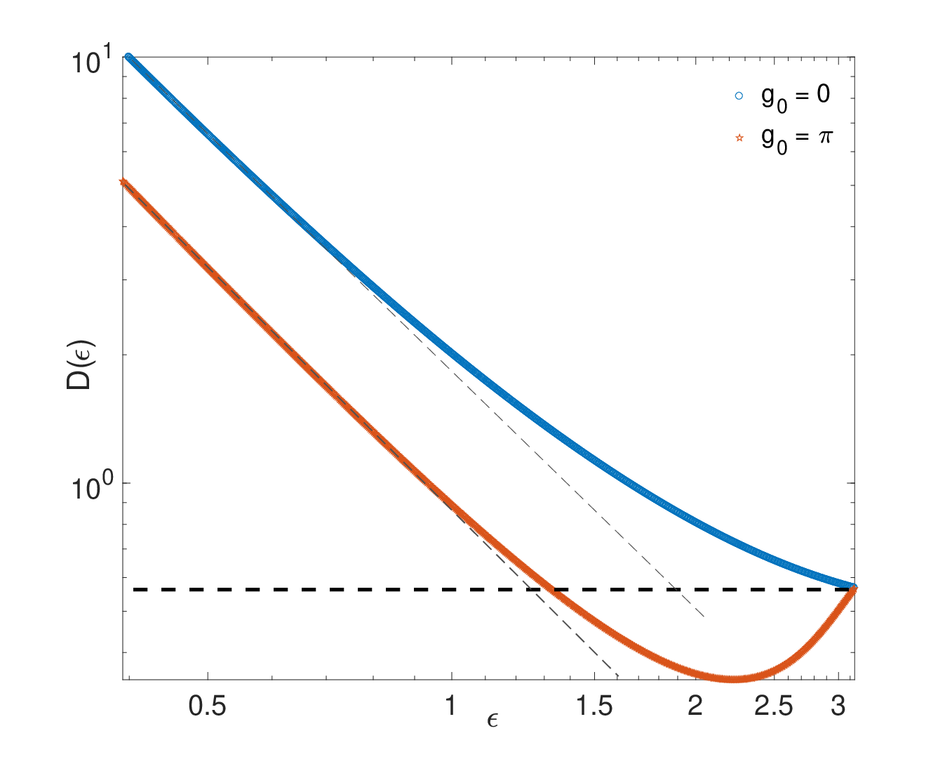
The main goal in this paper is the introduction of dynamical noise for the model described in the previous section. In order to see how the system responds to this kind of noise, we numerically simulate its evolution using the same equations as in the noiseless case, but randomly change the parameter at every step, from a uniform distribution, within the interval ], where is the center of the distribution. The entire procedure is repeated over a number of iterations, and the result is averaged over these samplings. As we discuss in the Appendix, this procedure is equivalent to a description in terms of a Lindblad operator acting on the density matrix that describes the state of the system. Using this, one can compute the asymptotic value of the diffusion constant, Eq. (34). The results are plotted on Fig. (2) for two values of , as a function of . As can be observed from the plots, rapidly falls for not too large values of . With , the curve deviates from the initial trend as approaches . The behavior for is different: has a minimum value at . Both curves have the same value when , given by .
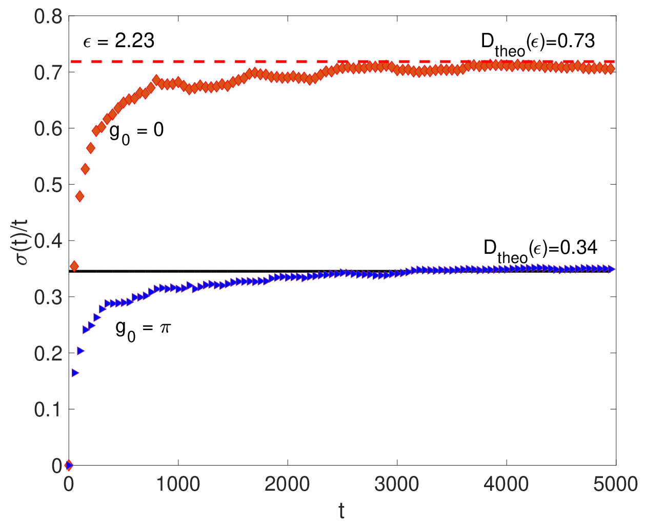
The approach to the asymptotic regime can be observed from Fig. (3). In this figure, we plot the evolution with time of the noisy QW, as numerically obtained following the procedure explained at the beginning of this Section, in comparison with our analytical result Eq. (34), for the value . We observe a good agreement between both approaches.
The strong decrease of the diffusion constant observed in Fig. (2) can be used to control the spreading of the QW, so that the wavepacket expands at very low speed, as compared with the usual noiseless case. Such decrease can, in principle, be further reduced by the use of a non-localized initial state, since this amounts to including the initial shape of the wavepacket in the integral Eq. (31).

Even more interesting is the study of the probability distribution, Eq. (3). We can observe how the probability concentrates around (see Fig. 4) . Differently from the case , for which we obtain the expected Gaussian solution, in the case we observe an exponential shape around zero. In fact, this evolution reminds us the phenomenon of Anderson localization. The result is intriguing due to the fact that dynamical noise is expected to transform the system into a classical random walk, but in this case we see some type of dynamical localization. Anderson localization has extensively been studied [20, 21, 22, 23] as the result of introducing a static disorder. It has also been studied in the context of quantum walks, see for example [16, 17]. What we obtained here, however, is a similar result, but produced by a time-dependent noise. This is the main result of our paper.
V Conclusions
In this paper, we investigated the role played by noise on the QW introduced in [1], a 1D model that is inspired by a two particle interacting QW. The noise is introduced by a random change in the value of during the evolution, from a constant probability distribution within a given interval. The consequences of introducing such kind of noise depend on both the center value and the width of that interval: a wider interval manifests as a higher level of noise. We observe that, by appropriately choosing the level of noise, one obtains a quasi-localized state, which a spreading rate can be made very small. The existence of this quasi-localized state for such kind of time-dependent noise is, to the best of our knowledge, totally new, since localization (i.e., Anderson localization) is linked in the literature to a spatial random noise.
VI Acknowledgements
This work has been supported by the Spanish Ministerio de Educación e Innovación, MICIN-FEDER project FPA2014-54459-P, SEV-2014-0398 and Generalitat Valenciana Grant GVPROMETEOII2014-087.
Appendix A Appendix: Diffusion constant
In this Section we analyze the long term behavior of the diffusion constant. Our calculation closely follows the formalism presented in [24, 25]. However, the dynamics of the decoherent QW will be represented by a matrix acting on four-vectors, instead of a superoperator. At a given time, the state of the system is defined, in quasi-momentum space by the vector
| (10) |
where , is the density operator at time step , and is the 2-dimensional identity, while , are the Pauli matrices. The trace in the latter equation is performed on the spin space. The above equation can be inverted to give
| (11) |
The probability distribution at time t can be obtained from
| (12) |
For a given sequence of choices , the time evolution of the density operator is obtained as
| (13) |
where . We now assume that the above sequence is randomly obtained from an interval with an uniform probability distribution if , and otherwise. Under these assumptions, it has been proven [26] that, in the limit , Eq. (13) can be described by the action of a superoperator defined as
| (14) |
so that
| (15) |
We can recast the latter equation under algebraic form (with vectors and matrices) by the use of Eq. (11). Then the vector defined in Eq. (10) evolves according to
| (16) |
where is a matrix defined as
| (17) |
with . We are interested in deriving an analytical expression for the variance
| (18) |
for large values of the time step . The initial state is assumed to be localized at , therefore
| (19) |
where is the initial coin state. Then
| (20) |
is independent of both and , with . Following similar steps as in [25], one arrives to
| (21) | |||||
with the convention of sum over repeated indices, and the following definitions
| (22) |
It can be shown that
| (23) |
The same property holds for . Use was made of these properties in deriving Eq. (21). Therefore, we can write in block-diagonal form
| (24) |
being a matrix. This structure is obviously preserved with time, i.e.
| (25) |
The explicit form of is cumbersome for general values of . We will here concentrate on two particular cases, namely and . In both cases, one can write
| (26) |
with the definitions and . The coefficients depend both on the value of and . We have dropped this dependence for simplicity. For one has , , , , and , while for we found , , , , and . We have introduced the notations , . The last term in Eq. (21) can be easily evaluated, resulting in
| (27) |
Starting from Eq. (26), one obtains that . Therefore, the first two terms in Eq. (21) can be combined to give
| (28) |
Moreover, one can check that,
| (29) |
does not depend on the action of , which allows us to drop this matrix off. Thus the integrand in Eq. (28) can be expressed in terms of the submatrix
| (30) |
We have verified that all the eigenvalues of obey , so that in the long time limit. Therefore, the last term in Eq. (30) will be time-independent at large time steps. In what follows, we will omit that term, since it does not affect our conclusions. The rest of the calculation is straightforward, and we obtain
| (31) |
where
| (32) |
with , , , and . The integral in Eq. (31) can be expressed in terms of standard integrals [27]. By defining , we arrive at the result:
| (33) |
From here, we define the diffusive constant
| (34) |
References
- [1] A. Ahlbrecht, A. Alberti, D. Meschede, V. B. Scholz, A. H. Werner, and R. F. Werner, New Journal of Physics 14 (2012), 10.1088/1367-2630/14/7/073050, arXiv:1105.1051 .
- [2] G. Grossing and A. Zeilinger, Complex Systems 2, 197 (1988).
- [3] N. Z. Y. Aharonov, L. Davidovich, Physical Review A 48, 1687 (1993), arXiv:1207.4535v1 .
- [4] D. A. Meyer, Journal of Statistical Physics 85, 551 (1996).
- [5] J. Kempe, Contemporary Physics 44, 307 (2003), arXiv:0303081v1 [quant-ph] .
- [6] I. Bloch, J. Dalibard, and S. Nascimbene, Nature Physics 8, 267 (2012).
- [7] A. Ambainis, International Journal of Quantum Information 1, 507 (2003).
- [8] F. Magniez, A. Nayak, J. Roland, and M. Santha, SIAM Journal on Computing 40, 142 (2011).
- [9] T. Kitagawa, M. A. Broome, A. Fedrizzi, M. S. Rudner, E. Berg, I. Kassal, A. Aspuru-Guzik, E. Demler, and A. G. White, Nature communications 3, 882 (2012).
- [10] P. Arnault, G. Di Molfetta, M. Brachet, and F. Debbasch, Phys. Rev. A 94, 012335 (2016).
- [11] M. Genske, W. Alt, A. Steffen, A. H. Werner, R. F. Werner, D. Meschede, and A. Alberti, Physical review letters 110, 190601 (2013).
- [12] A. Schreiber, A. Gábris, P. P. Rohde, K. Laiho, M. Štefaňák, V. Potoček, C. Hamilton, I. Jex, and C. Silberhorn, Science 336, 55 (2012).
- [13] R. Côté, A. Russell, E. E. Eyler, and P. L. Gould, New Journal of Physics 8, 156 (2006).
- [14] D. A. Meyer, International Journal of Modern Physics C 08, 717 (1997).
- [15] L. Sansoni, F. Sciarrino, G. Vallone, P. Mataloni, A. Crespi, R. Ramponi, and R. Osellame, Physical review letters 108, 010502 (2012).
- [16] A. Joye and M. Merkli, Journal of Statistical Physics 140, 1025 (2010).
- [17] A. Ahlbrecht, V. B. Scholz, and A. H. Werner, Journal of Mathematical Physics 52, 102201 (2011a), http://dx.doi.org/10.1063/1.3643768 .
- [18] M. a. Nielsen and I. L. Chuang, Cambridge University Press (2011) p. 702, arXiv:arXiv:1011.1669v3 .
- [19] A. Ambainis, E. Bach, A. Nayak, A. Vishwanath, and J. Watrous, Proceedings of the thirty-third annual ACM symposium on Theory of computing 3, 37 (2001).
- [20] F. Evers and A. D. Mirlin, Reviews of Modern Physics 80, 1355 (2008), arXiv:0707.4378 .
- [21] A. Lagendijk, B. Van Tiggelen, and D. S. Wiersma, Phys. Today 62, 24 (2009).
- [22] A. Ahlbrecht, H. Vogts, A. H. Werner, and R. F. Werner, Journal of Mathematical Physics 52, 042201 (2011b), http://dx.doi.org/10.1063/1.3575568 .
- [23] A. Joye, Communications in Mathematical Physics 307, 65 (2011).
- [24] T. Brun, H. Carteret, and A. Ambainis, Physical Review A 67, 032304 (2003), arXiv:0210180 [quant-ph] .
- [25] M. Annabestani, S. J. Akhtarshenas, and M. R. Abolhassani, Phys. Rev. A 81,, 032321 (2009), 0910.1986 .
- [26] G. Di Molfetta and F. Debbasch, Quantum Studies: Mathematics and Foundations 3, 293 (2016).
- [27] I. Gradshteyn and I. Ryzhik, Table of integrals, series, and products, 7th ed. (Academic Press, 2007).