Truthful Spectrum Auction for Efficient Anti-Jamming in Cognitive Radio Networks
Abstract
One significant challenge in cognitive radio networks is to design a framework in which the selfish secondary users are obliged to interact with each other truthfully. Moreover, due to the vulnerability of these networks against jamming attacks, designing anti-jamming defense mechanisms is equally important. In this paper, we propose a truthful mechanism, robust against the jamming, for a dynamic stochastic cognitive radio network consisting of several selfish secondary users and a malicious user. In this model, each secondary user participates in an auction and wish to use the unjammed spectrum, and the malicious user aims at jamming a channel by corrupting the communication link. A truthful auction mechanism is designed among the secondary users. Furthermore, a zero-sum game is formulated between the set of secondary users and the malicious user. This joint problem is then cast as a randomized two-level auctions in which the first auction allocates the vacant channels, and then the second one assigns the remaining unallocated channels. We have also changed this solution to a trustful distributed scheme. Simulation results show that the distributed algorithm can achieve a performance that is close to the centralized algorithm, without the added overhead and complexity.
Index Terms:
Cognitive Radio Network, Zero Sum Game, Auction, Learning, Anti-Jamming Scheme.I Introduction
Spectrum scarcity has been a major problem for the existing wireless networks which motivated researchers to investigate new intelligent paradigm to manage available spectrum. Cognitive radio (CR) has thus emerged as a promising approach to improve spectral efficiency in wireless networks. In CR networks, secondary users (SUs) may cognitively access unused spectrum that is not currently occupied by licensed users, namely primary users (PUs) under the condition that the PUs’ transmission will not be interfered [1].
Spectrum management in CR networks has been considered in many recent works such as [2] and [3] (and references therein). One important technique that enables CR-oriented spectrum allocation is to consider spectrum auction among SUs that seek to idle channels [4]. Auction theory, which is rooted in economics, offers a promising solution for intelligently allocating resources, such as power and spectrum, in CR networks. There are different approaches for implementing auction theory in wireless networks, which have been investigated in [5]. In general, in such scenarios, users are rational and have their own strategies in order to get more resources. Extensive existing works are available on different auction approaches for spectrum allocation (e.g., see [6]). For instance, the authors in [7] find the maximization of the PUs’ expected profit by proposing the leasing based spectrum allocation for SUs. In addition, the first price auction to optimize both the total payoff of SUs and revenue of auctioneer is studied in [8]. One drawback of the suggested scheme is that SUs might reveal wrong to further improve their utilities. The work in [9] provides a spectrum allocation based upon a double-sided auction mechanism. In this scheme, an untruthful behavior also brings suboptimal solutions.
Competition among the selfish SUs is crucial to use rare resources in the spectrum market framework [10]. More importantly, non-cooperative users have intentions to cheat so as to gain more benefits. The Vickrey Clarke Groves (VCG) auction mechanism is commonly used in the auction games in order to provide not only the assurance of truthfulness but also the maximization of the social welfare [11]. For example, the authors in [12] and [13] proposed the incentive mechanism to encourage users to contribute truthfully their resources by forming coalitions. Moreover, because of selfishness of SUs, each user attending in the auction has incomplete information about the other users. Hence, selecting a proper learning task is a big challenge for designing the distributed game. A Bayesian nonparametric belief update scheme is suggested to solve this issue in [14].
In CR networks, SUs are susceptible to several malicious attacks. Several anti-attack mechanisms have been proposed in existing literature [15]. For example, the problem of PU emulation attack on CR networks has been investigated in [16] in which a malicious user can send signals with the same PU transmission characteristics in order to mislead the SUs. Instead, SUs can recognize PUs’ transmission by adapting a favorable verification protocol. In addition, a game-theoretic approach based upon the concept of secrecy capacity is proposed to model eavesdropping attacks on CR networks in [17]. In [18], a set of SUs is available in a stochastic medium and they select randomized channel hopping as the defensive strategy. This framework falls into the category of the zero sum stochastic game and the authors propose a minimax-Q learning to find the related solution. Besides, the randomized defense strategy for channel hopping and power allocation with learning algorithms is suggested in [19]. However, in a spectrum auction, users act selfishly and these defense strategies are not fully applicable.
The main contribution of this paper is to jointly consider truthful spectrum auction and the presence of a jamming attack. In this scenario, two types of users exist: selfish SUs participating the auction and a malicious jamming user that wishes to reduce the social welfare as much as possible. Our key contributions can therefore be summarized as follows:
- •
To model the mentioned scenario, we formulated two inter-related games: a zero-sum stochastic game between the CR network and the jammer, and an associated mechanism design among the SUs at each stage of the game. Indeed, the zero sum game exists between the CR network and the malicious user, while mechanism design is considered among the SUs. Using our proposed framework, the SUs do not show their selfishness and at the same time cooperate with each other to get higher profits against the malicious user.
- •
In order to realize the joint games, we propose an algorithm based on zero-sum game which can extensively reduce the complexity of solving the game with an asymmetric number of actions for the players. The proposition is a basis for the work because the malicious user and the SUs are unequal in the number of actions.
- •
Using the derived proposition, we show that the zero-sum stochastic game and spectrum auction game can be converted to a centralized two-level spectrum auction in which SUs send their bids to a coordinator and the coordinator confronts against the malicious user. More specifically, the coordinator initially allocates spectrum to the first level bids, and then the remaining spectrum is allocated by the second auction. Indeed, the main idea of the centralized two-level auction is inspired from the randomized auction which is common in combinatorial auction theory such as [20] and [21]. However, our considered scenario significantly differs from those existing works.
- •
A decentralized method based upon the centralized two-level auction is examined. The proposed algorithm use the proven interesting properties of the centralized game which extremely reduces the complexity of the game. Simulation results show that the loss in performance for the decentralized method in comparison with the centralized one is negligible.
- •
Due to the fact that SUs have no knowledge about the states of other SUs and jammer, the parameters for the decentralized scheme must be learnt from a proper scheme like the one proposed in [22]. We propose a Boltzmann-Gibbs algorithm to estimate the unknown parameters for each users. Simulation results show that this method yields considerable performance gains. Moreover, the convergence of the proposed decentralized game can be controlled by learning parameters.
The rest of this paper is organized as follows. The system model is presented in Section II. In Section III, a centralized algorithm based on a two-level auction is described. In Section IV, we propose a truthful decentralized method in accordance with the proposed centralized auction. The simulation results are given in Section V. Finally, in Section VI, we conclude the paper.
II System Model and Protocol Description
We consider a CR network consisting of channels having a slotted-time structure indexed by . Moreover, the duration of each time-slot is assumed to be . There are SUs that seek to access the vacant channels to send their data. Moreover, these users are selfish and non-cooperative. The primary network consists of a number of PUs who have a have priority to use the channels in a slotted-time manner. We consider an on-off scheme to model the channel usage, in which and indicate that channel is idle and busy at time , respectively [18] and [19]. The transition probabilities from on-to-off and off-to-on are and , respectively. Without loss of generality, we assume that every SU can only use one channel at time [23]. In order to avoid the conflict with the PUs transmission, each SU knows the availability of all the channels before transmitting. This can be done by using wideband sensing or cooperative sensing techniques [24].
The state of channel for SU is assumed to be the received signal-to-noise-ratio (SNR) , following an exponential distribution with mean of . Similar to [25], we represent by discrete states to attain a finite Markov chain. In addition, let indicate the buffer state of user at time and where is the maximum buffer size. Thus, the state of SU at time is and the state of the stochastic game is described as follows:
| (1) |
where the state of the game consists of the state of each SU and the occupancy state of each channel. The assigned channel to the -th SU is denoted by . Moreover, it is possible that no channel is assigned to the SU, i.e., . Thus, we have .
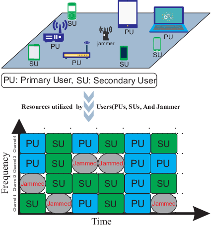
Assume there is a malicious attacker in this scenario which attempts to interrupt the communication links of the SUs by inserting interference. The action of malicious user is to jam channels chosen from the vacant channels. Indeed, if the malicious user jams channel , the communication link is assumed to be disrupted at that time. We assume that the jammer knows the channel occupancy states at each stage time. For simplicity, we assume , and our approach can be extended to case. The action of jammer, , indicates the jammed channel by the attacker. Fig. 1 shows the proposed system model and illustrates how users occupy the time-frequency resources.
Notice that the availabilities of the channels are only imposed by PUs, and hence, they are independent of the attacker’s action and SUs’ actions. Consequently, we can now derive the transition probability of the states as
| (2) | |||
includes information about the channels’ conditions and the buffer state. The channel conditions do not depend on the SUs action. Besides, the buffer state, , is affected by the jammer action, , the action of SU , , and . Hence, we can express the last term of (2) as
| (3) |
We denote the incoming traffic of SU at time as where . It is assumed that has the Poisson distribution with the average [23]. Moreover, the buffer state is derived from . Hence, we have the following expression for its transition probability
| (4) |
where and indicates the transmission bit rate if channel is selected and channel is jammed. Therefore, can be calculated as [32]
| (6) |
where , and are the time duration, bandwidth of each channel and target bit error rate, respectively. In (5), and indicate the largest integer number which is lower than and the sign of , respectively. When the -th SU selects channel and the jammer selects the -th channel at the same time, the utility function of user at time is characterized as follows
| (7) |
In our scenario, we consider the presence of a coordinator that allocates spectrum to the SUs according to the submitted bids while maximizing the worst-case social welfare corrupted by the attacker. Hence, the interactions between the coordinator and the SUs are cast as an auction with the following elements:
- •
The auctionees are the SUs which aim at using the vacant channels.
- •
The auctioneer is the coordinator which allocates the channels to SUs. Afterwards, the auctioneer and coordinator are used interchangeably.
- •
Each bid is denoted by , where . Here, indicates the proper bid for SU to use channel while the attacker jams channel .
- •
The following constraints must be satisfied at each stage of the auction:
in which shows that channel is allocated to the -th SU if ; and is not allocated otherwise.
In order to combat the jammer, the coordinator should assign the channels to the SUs via a random strategy. In the next section, we will investigate this optimal strategy.
III Anti-Jamming Decentralized Game Based on Learning Process
In the previous section, the PC-game is proposed in order to extract the anti-jamming mechanism under the condition that all SUs and the auctioneer act as one player to defeat the malicious user. However, this assumption may not hold in general since the SUs are selfish and maybe untruthful. Unreliable information may lead to an improper strategy for protection of the SUs against the jammer. Besides, the SUs send their bids to the coordinator, which has the high complexity. Due to these drawbacks, this section suggests a decentralized method according to the framework provided by the PC-game.
In the PC-game, we use a two level auction, and our aim is to specify a distribution function to the actions. These actions can be recognized by the first and second preferences of all the SUs. First, pay attention to where and are the optimal policies of the auctioneer and the jammer, respectively. Moreover, and are the -th entry of and the -th row of payoff matrix of the original game in Definition 1. If we extend each into its elements, we have the following formulation:
| (11) |
in which is equal to the probability of selection of the -th channel for the -th user. Every policy, which yields the same , is the optimal strategy against the attacker. This fact motivates us to move from the PC-game to a distributed game. In the PC-game, we specify a probability to each action distinguished by the first auction or equivalently the first preferences of the SUs. By truthfulness assumption and help of the mentioned fact, if each SU individually estimate the probabilities connected with the preferences over the channels, then the value of the PC-game obtained from (14) can be approximated by the following formulation:
| (12) |
where and are the estimated probability related to the first preference by the -th SUand the value of the game when the SUs’s preferences are , respectively.
Each auction consists of allocations to the SUs. Note that from Proposition , we only need auctions to reach to the best response against the jammer. Thus, there are at most important probabilities, , at each stage of game. Moreover, it can be easily demonstrated that every policy, which has these probabilities, is optimal from the perspective of the zero-sum game. On the other side, each SU has control over probabilities for stating its first preference over the channels. From this point of view, the SUs have variables for estimations of important probabilities which are improved with increasing compared to .
At this time, by applying the auction feature to the game, the coordinator can get payments from the SUs. The payment of each SU is constructed from two parts. One payment part is related to the first-auction and the other part is associated with the second-auction. The computation approach of the payment for the first-auction which is similar to [23]is stated as
| (13) |
in which is the solution of the first auction. For the second-auction, this payment can also be computed by the same procedure while the selected SUs in the first-auction and their corresponding announced bids are omitted by the coordinator. The PD-game procedure is described in Table I. We show these payments oblige the SUs to bid truthfully. In order to prove that the proposed distributed game (PD-game) contains the truthful mechanism, first we define the concept of truthfulness in expectation.
Definition 1
Assume , , and are the real value of bid for user , the announced value of bid for user , the value of bids for other users and the payment assigned to user , respectively. A mechanism is truthful in expectation when for any user and any of other users, the expectation of profit attained by user , is maximum if [28].
We now focus on a proposition which states that the PD-game is truthfulness in expectation.
Proposition 1
The proposed procedure for assigning payment satisfies truthfulness in the expectation criterion.
Proof:
The proof is given in Appendix C. ∎
Note that the payment of each SU, which is dependent on all the SUs’ bids, converts the profit gained by each SU into a notion of the overall value of the zero-sum game. Thus, we are trying to model the game between each SU and the attacker as the zero-sum game separately so that the separate game for each SU has some external factors related to other SUs, and each SU is effective only on a certain amount of the profit.
By doing so, every SU computes the distribution of stating its preference over the channels. In addition, the communication burden of stating its bids obviously plummets. Since, the SU only sends bids instead of stating . Duties of the coordinator decreases since it only computes the first and second-auctions and their related payments. Indeed, the utility matrix of the separate game between each SU and the attacker is modeled as a matrix because the SU has choices for the announcement of its first preference.
| Step 1. The SUs submit the bid based upon (12) to the coordinator. At the same time, the SUs announce their preferences over |
| channels in order to be used in the first and second auctions. |
| Step 2. First auction is computed for the first preferences of the SUs. Then, allocation and payment for each SU is assigned to |
| them by using (7) and (16). |
| Step 3. Similarly, the second auction is computed for the remaining channels and the SUs. |
Note that our algorithm is distinct from work suggested in [30] in which authors employ a factored approximation of the overall Q-function based upon the linear combination of users’ Q-function for the stochastic game. The proposed algorithm is not applicable in our scenario because the SUs are selfish and interested in benefiting further. Indeed, the payment structure makes the profit of SUs’ network directly relevant to each individual profit due to Proposition . Instead, is estimated by SUs’ probabilities, .
The fundamental difficulty of the PD-game is that each SU does not know enough about its related separate utility matrix. Remembering that the game will be repeated infinitely, and therefore, the SUs can learn their utilities by a certain learning scheme. We employ the scheme proposed in [22]. The advantage of this scheme is that each SU can adapt different patterns of learning. The probabilistic strategy over the actions and utility of each stage can be learned through the game. First, we apply an iterative Boltzmann-Gibbs strategy which is stated as
| (14) |
where and are distribution of selecting channel as the first preference of SU and the estimated average payoffs updated at iteration , respectively [22]. Next, we update distribution and payoff, respectively, as
| (15) | |||
| (16) |
in which is the profit gained by SU at time when selecting channel as its preference, which is zero when no channel is assigned to it, and is when channel is assigned. Furthermore, and are the learning rates indicating players’ capabilities of information retrieval and update. Therefore, each SU can learn the distribution over its preference from implementing a Q-learning based method. It can be proved that Q-learning method converges to the optimal solution for only single-agent case; However, there is no such a guarantee for multi-agent cases [29]. In the next section, simulation results illustrate the convergence of the PD-game to the sub-optimal solutions.
IV Simulation results
In this section, we provide simulation results to verify the truthful anti-jamming network. We consider a cognitive radio environment with channels, secondary users and a malicious user. We assume that the state of signal to noise ratio for SU and channel , , has three values and . The probability of state transitions from these states are , , , , , and . In addition, and for . We set also for all the users in (5) as .
IV-A Convergence
The convergence speed of the PC-game and the PD-game for three SUs are investigated in Fig. 2 and Fig. 3 when and , respectively. Besides, and for all SUs for the either case. The normalized cumulative value of SUs is used as a convergence comparison tool. As Fig. 2 and Fig. 3 report, both algorithms converge; however, the PD-game takes longer time to reach the stable solution. The PD-game is done in the decentralized scheme with incomplete information. Therefore, it needs more times to learn the unknown parameters. In particular, the convergence rates in Fig. 3 for both the PC-game and PD-game are quite slower than those in Fig. 2. Indeed, increase in leads to rises in the numbers of the states and the complexity of the system. Consequently, the required numbers of iterations in Fig. 3 explicitly becomes greater.


The learning parameters , and in (17), (18) and (19) play important roles in the convergence of the PD-game. In [22], it is shown that for assurance of the convergence. Hence, we consider where is the repetition numbers of state occurrence, where . Fig. 4 depicts the effect of different and on the iterations required for the convergence under the mentioned condition when . It is clear that when these parameters increase, the convergence speed decrease, since the impact of instantaneous utilities on current strategy decreases.
IV-B The effects of SU parameters on performance
In this part, the effects of the maximum allowable , the number of channels , and the number of users on the PD-game and the PC-game are evaluated. In order to have a similar benchmark for comparison of two methods, we define a new parameter based on (6) as,
Fig. 5 and Fig. 6 illustrate the performance of the PC-game and the PD-game by for variable and when and , respectively. The other parameters are set alike to the previous part. In Fig. 5, the SU with the greater is able to hold the data for a longer time. Thus, the increment in decreases . In other words, it can improve the performance of the system. However, increase in has opposite impact on the which is result of increasing the dropping probability of data. Moreover, Fig. 6 shows the performance when . Note that both the PC-game and PD-game in Fig. 6 have lower rather than those in Fig. 5 for the same condition. Indeed, increases the opportunities of available vacant channels for each SU; therefore, decreases the numbers of unsent buffered information.


The performance of the scenario for different average of incoming traffic and the numbers of SUs is shown in Fig. 7 and Fig. 8. The results are obtained for and , respectively. Rise in means that the average of incoming traffic increase. The outcome of the rise is to receive more traffic data at each stage of the game; as a result, the average unsent traffic increase. Finally, Fig. 9 displays versus when . Notice that increase in along with causes to be lower which validates our discussion about the performance of the scheme.
V Conclusion
Spectrum management among the SUs is a vital issue for CR networks, and auction theory provides a helpful tool to allocate spectrum to SUs. In this article, first, we proposed a centralized two-level auction which combined both the advantages of efficient resource assignment to SUs and acting against the malicious user. Next, a proposition for the zero-sum game was given which can be applied in a game with the non-uniform number of users’ actions. More importantly, we introduced a decentralized protocol based upon the centralized method properties and the mentioned proposition. The decentralized scheme obliges SUs to bid truthfully because SUs can gain higher profit in expectation for the long-term interaction. Simulation studies show that both the centralized and decentralized scheme converge in the limited numbers of stages. Moreover, the performance of the proposed approach are comparable with the efficient centralized solution.
Appendix A Proof of Proposition 1
Consider a zero-sum game with payoff matrix as follows
| (17) |
in which shows that player and player obtain and profitwhen they select their -th and -th actions, respectively. To attain the optimal solution [26], we should consider mixed strategy with the help of the following equation:
| (18) |
where and indicate the probability distributions over the related actions of player and player , and is the value of the game. Moreover, can be expressed as,
where is vector for
. Hence, and
. In addition, we consider all the entries of matrix are more than zero. The value of the game, which contains actions with vectors
, is denoted by
.
First, we state a lemma in order to prove the proposition.
Lemma 1
If the following relationship exists between , player can play the game without the -th action while it gets the same value,
| (19) |
Proof:
First, assume that player has optimal probabilities over , respectively. Equation (22) can be rewritten by the following representation,
where the following relationships exist between the set of s and s
Moreover, we have the next equations between and for ,
| (20) |
Afterwards, we introduce a game containing actions with vectors and . Besides, the optimal probabilities of the new game are assumed as and . The value of game to which the -th action is added is not less than the game without the -th action according to [31], meaning that,
| (21) |
In other words, for the new game, we have the following results,
where finds the entry with the minimum value of vector . If both and are not less than zero, set can be interpreted as a distribution vector over actions of player . Notice that each probability distribution over these selected actions brings the value not greater than . Thus, we can conclude that
| (22) |
Due to (24) and (25), we have
| (23) |
In other words, if the action with vector is eliminated, we will gain the same value. However, if one of them is less than zero, we cannot get the above formulation. Without loss of generality, we assume that and . Remind that , thus and therefore . Because the summation over probabilities is 1, hence,
Now, consider distribution vector which is constructed by the following,
| (24) |
where . Again, we have the following inequality:
| (25) |
To put it differently, (28) can be reformulated as
Besides, (24) gives that
and,
If , and are the -th the entries of , and , respectively, we could obtain the following result,
| (26) |
Consequently,
| (27) |
This suggests the following inequality for , and
| (28) |
Therefore, consideration of both (30) and (31) gives us the following inequality,
| (29) |
in which , , ,. We know that the minimum entry of vector is not higher than for any set of , ,. Therefore, our initial assumption is not correct. In other words, is not less than zero, and we can obviate . It means that
| (30) |
Returning to the general case in (22), it can be concluded from (33) that
| (31) |
∎The expression in (34) states that if satisfies the conditions of Lemma 1, we can omit it. Here, we return to prove Proposition . Each has entries, so we can represent all of the vectors by at most vectors of them. These basic vectors are linear and independent. Without loss of generality, we assume that these vectors are where . Based upon the vector representation, all s are classified into three groups.
Now, we assume that each can be displayed by . Also, the coefficients are unique due to linearity and independency. These groups are stated as follows:
Group I: If , we can obviate and get the same value as in Lemma 1.
Group II: If , we have the following facts:
We assume that the optimal probability distributions over the actions are .
where the second term does not include . From [26], we know that
| (32) |
Now, we extend (35) as
in which we call the expression stated in parenthesis in the last term as . The value of the game when playing with instead of is given via
Now, can be represented by basic vectors in which the sum of coefficients becomes . Thus, we can obviate and at the same time get the same value. In other words, we have
Moreover, we have
Then, we can remove all of vectors which have coefficients satisfying the following inequality without loss in the value of the game, .
| (33) |
Group III: If , we can show by the following equation
| (34) |
In this case, there exists at least one coefficient, e.g., , which is greater than zero. Now, we try to show by including . Indeed,
However, we know that
| (35) |
Therefore, we can remove according to the second group. As a result, we only need the actions among the onesand get the same value. Similar classification can be applied to vectors of and at each stage one vector is removed. Finally, actions (vectors) remain for playing the game.
Appendix B Proof of Proposition 2
First, we consider an assumption for each allocation to continue our proof.
Assumption 1
If the following relation exist between vectors of allocations, ,
| (36) | |||
then the occurrence probability of all relations is zero.
Indeed, each has entries. Accordingly, the allocation vectors construct equations, and we have parameters involving . For (39), we have parameters satisfying equations. This situation makes hard to yield these parameters out of equations. For instance, if each is independent with respect to the other with the uniform distribution, this assumption is precise. Also, our simulation result certifies the assumption. We assume that the attackers strategy is the same as the strategy of the original zero-sum game. In the original form, we have the following equation
inwhichp^*_1p^*_2Uu_imax(u_1,…,u_ N! (N-M’)! )M’M’^(N-M’)JJ(1,2,…,M’)(1,2,…,M’,j,…,j)JjM’+1M’h_ o_iM’+1
Appendix C Proof of Proposition 3
In the PD-game, payment for user has two parts, and , which are related to first and second auctions. If we assume that the SUs choose preferences as their actions and channel is dedicated to the -th SU while the attacker jams channel , we have the following formulation for the average profit of SU .
| (43) |
In (42), and are the actual and submitted bid for SU . Moreover, , and are the probability for jamming of channel by the jammer, the set of SUs and channels remained from first auction, respectively. To attain the -th user’s profit, we should apply the probability of preferences for all the SUs. Moreover, , therefore, similar to . Hence, the expectation profit can be stated as follows,
| (44) |
Equivalently,
| (45) |
The third and fourth terms are not function of the -th SU. Therefore, we can disregard them to further analysis. But, the summation over the first and second terms are equal to the total profit of the SUs according to . In other words, the individual profit is equivalent to the total profit. For this reason, the rational SUs must bid truthfully.
References
- [1] Q. Zhao and B. M. Sadler, “A Survey of Dynamic Spectrum Access: Signal Processing, Networking, and Regulatory Policy,” IEEE Signal Processing Mag., vol. 24, no. 3, pp. 79-89, May 2007.
- [2] E. Hossain, D. Niyato, and Z. Han, Dynamic Spectrum Access in Cognitive Radio Networks, Cambridge University Press, 2009.
- [3] G. I . Tsiropoulos, O. A. Dobre, M. H. Ahmed, and K. E. Baddour, “Radio Resource Allocation Techniques for Efficient Spectrum Access in Cognitive Radio Networks,” IEEE Communications Surveys Tutorials, no. 99, 2014.
- [4] Z. Li, B. Li, and Y. Zhu, “Designing Truthful Spectrum Auctions for Multi-hop Secondary Networks,” in IEEE Trans. Mobile Comput., vol. 14, no. 2, pp. 316-327, Feb. 2015.
- [5] Y. Zhang, C. Lee, D. Niyato, and P. Wang, “Auction Approaches for Resource Allocation in Wireless Systems: A Survey,” IEEE Communications Surveys and Tutorials, vol. 15 , no. 3, pp. 1020-1041, Third Quarter 2013.
- [6] N. Zhang, H. Liang, N. Cheng, Y. Tang J. W. Mark, and X. S. Shen, “Dynamic Spectrum Access in Multi-Channel Cognitive Radio Networks,” IEEE Journal on Selected Areas in Communications, vol. 32, no. 11, pp. 2053-2064, Nov. 2014.
- [7] X. Cao, Y. Chen, and K. J. R. Liu, “Cognitive Radio Networks With Heterogeneous Users: How to Procure and Price the Spectrum?,” IEEE Transactions on Wireless Communications, vol. 14, no. 3, pp. 1676-1688, Mar. 2015.
- [8] M. Tehrani and M. Uysal, “Auction Based Spectrum Trading for Cognitive Radio Networks,” IEEE Communications Letters, vol. 17, no. 6, pp. 1168-1171, May 2013.
- [9] W. Yong, Y. Li, L. Chao, Chonggang Wang and Xiaolong Yang, “ Double-Auction-Based Optimal User Assignment for Multisource Multirelay Cellular Networks ,” IEEE Transactions on Vehicular Technology, vol. 64, no.6, pp. 2627-2636, Jun. 2015.
- [10] Z. Han, D. Niyato, W. Saad, T. Basar, and A. Hjorungnes, Game Theory in Wireless and Communication Networks: Theory, Models and Applications , Cambridge University Press, 2011.
- [11] W. Vickrey, “Counter Speculation, Auctions, and Aompetitive Sealed Tenders,” Journal of Finance, vol. 16, no. 1, pp. 8-37, Mar. 1961.
- [12] C. Yi and J. Cai, “Multi-Item Spectrum Auction for Recall-Based Cognitive Radio Networks With Multiple Heterogeneous Secondary Users,” IEEE Transactions on Vehicular Technology, vol. 64, no. 2, pp. 781-792, Feb. 2015.
- [13] J. Ma, J. Deng, L. Song, and Z. Han, “Incentive Mechanism for Demand Side Management in Smart Grid Using Auction,” IEEE Transactions on Smart Grid, vol. 13 , no. 1, pp. 75-88, Jan. 2014.
- [14] Z. Han, R. Zheng, and V. H. Poor, “Repeated Auctions with Bayesian Nonparametric Learning for Spectrum Access in Cognitive Radio Networks,” IEEE Transactions on Wireless Communications, vol. 10, no. 3, pp. 890-900, Mar. 2011.
- [15] M. H. Manshaei, Q. Zhu, T. Alpcan, T. Bacsar, and J. P. Hubaux, “Game Theory Meets Network Security and Privacy,” Ecole Polytechnique F´ed´erale de Lausanne (EPFL), Tech. Rep. EPFL-REPORT-151965, Sep. 2010.
- [16] A. G. Fragkiadakis, E. Z. Tragos, and I. G. Askoxylakis, “A Survey on Security Threats and Detection Techniques in Cognitive Radio Networks,” IEEE Communications Surveys Tutorials, vol. 15, no. 1, pp. 428-445, 2013.
- [17] A. Chorti, S. M. Perlaza, Z. Han, and H. V. Poor, “On the Resilience of Wireless Multiuser Networks to Passive and Active Eavesdroppers,” IEEE J. Sel. Areas Commun., vol. 31, no. 9, pp. 1850-1863, Sep. 2013.
- [18] B. Wang, Y. Wu, and K. J. R. Liu, “An Anti-jamming Stochastic Game in Cognitive Radio Networks,” IEEE J. Sel. Areas Commun., vol. 29, no. 4, pp. 877-889, Apr. 2011.
- [19] Y. Wu, B. Wang, K. J. R. Liu, and T. C. Clancy, “Anti-Jamming Games in Multi-Channel Cognitive Radio Networks,” IEEE J. Sel. Areas Commun., vol. 30, no. 1, pp. 4-15, Jan. 2012.
- [20] Z. Li, B. Li, and Y. Zhu, “Designing Truthful Spectrum Auctions for Multi-hop Secondary Networks,” IEEE Transactions on Mobile Computing, vol. 14, no. 2, pp. 316-327, Feb. 2015.
- [21] H. Huang, Y. E. Sun,X. Y. Li, S. Chen, M. Xiao, and L. Huang, “Truthful Auction Mechanisms with Performance Guarantee in Secondary Spectrum Markets,”IEEE Transactions on Mobile Computing, vol. 14, no. 6, pp. 1315-1329, June. 2015.
- [22] Q. Zhu, H. Tembine, and T. Basar, “Heterogeneous Learning in Zero-sum Stochastic Games with Incomplete Information,” in Proc. 49th IEEE Conf. Decision Control, Atlanta, GA, Dec. 2010, pp. 219-224.
- [23] F. Fu and M. van der Schaar, “Learning to Compete for Resources in Wireless Stochastic Games,” IEEE Trans. on Vehicular Technology, vol. 58, no. 4, pp. 1904-1919, May 2009.
- [24] K. C. Chen, Y. J. Peng, N. R. Prasad, Y. C. Liang, and S. Sun, “Cognitive Radio Network Architecture: Part I-General Structure,” in Proc. ACM ICUIMC, Seoul, South Korea, pp. 114-119, Jan. 2008.
- [25] Q. Zhang and S. A. Kassam, “Finite-state Markov Model for Rayleigh Fading Channels,” IEEE Trans. Commun., vol. 47, no. 11, pp. 1688-1692, Nov. 1999.
- [26] T. Basar and G. J. Olsder, “Dynamic Noncooperative Game Theory,” 2nd edition, Classics in Applied Mathematics, SIAM, Philadelphia, 1999.
- [27] J. Robinson. “An Iterative Method of Solving a Game,” Ann. Math., vol .54, no. 2, pp. 296-301, Sep. 1951.
- [28] N. Nisan and A. Ronen, “Algorithmic mechanism design,” Games and Economic Behavior, vol. 35, no. 1-2, pp. 166-196, Apr. 2001.
- [29] H. J. Kushner, and G. Yin, Stochastic approximation and recursive algorithms and applications, Springer Science and Business Media, New York, NY, 2003.
- [30] C. Guestrin, D. Koller, and R. Parr, “Multiagent Planning with Factored MDPs,” In Proceeding of the 14th Neural Information Processing Systems (NIPS-14) , pp. 1523-1530, Vancouver, Canada, Dec. 2001.
- [31] D. Fudenberg and J. Tirole, Game Theory, MIT Press, Cambridge, MA, 1991.
- [32] Goldsmith and S.-G. Chua, “Variable rate variable power MQAM for fading channels,” IEEE Trans. Commun., vol. 45, no. 10, pp. 1218–1230, Oct. 1997.