跳到论文正文
W Papers独立论文阅读器 arXiv:1611.08561 论文正文 计算阅读时间 · 0%
引用这篇论文根据当前论文元数据生成,正式投稿前建议核对。


License: arXiv.org perpetual non-exclusive license
arXiv:1611.08561v8 [cs.IT] 17 Feb 2017

A Tight Rate Bound and a Matching Construction for Locally Recoverable Codes with Sequential Recovery From Any Number of Multiple ErasuresThanks: P. Vijay Kumar is also an Adjunct Research Professor at the University of Southern California. This research is supported in part by the National Science Foundation under Grant 1421848 and in part by an India-Israel UGC-ISF joint research program grant.Thanks: S. B. Balaji would like to acknowledge the support of TCS research-scholarship program.

S. B. Balaji, Ganesh R. Kini and P. Vijay Kumar, Fellow, IEEE Affiliation:  Affiliation: Department of Electrical Communication Engineering, Indian Institute of Science, Bangalore.
Email: balaji.profess@gmail.com, kiniganesh94@gmail.com, pvk1729@gmail.com
Affiliation: 
Abstract

An [n,k][n,k] code 𝒞\mathcal{C} is said to be locally recoverable in the presence of a single erasure, and with locality parameter rr, if each of the nn code symbols of 𝒞\mathcal{C} can be recovered by accessing at most rr other code symbols. An [n,k][n,k] code is said to be a locally recoverable code with sequential recovery from tt erasures, if for any set of s≤ts\leq t erasures, there is an ss-step sequential recovery process, in which at each step, a single erased symbol is recovered by accessing at most rr other code symbols. This is equivalent to the requirement that for any set of s≤ts\leq t erasures, the dual code contain a codeword whose support contains the co-ordinate of precisely one of the ss erased symbols.

In this paper, a tight upper bound on the rate of such a code, for any value of number of erasures tt and any value r≥3r\geq 3, of the locality parameter is derived. This bound proves an earlier conjecture due to Song, Cai and Yuen. While the bound is valid irrespective of the field over which the code is defined, a matching construction of binary codes that are rate-optimal is also provided, again for any value of tt and any value r≥3r\geq 3.

Index Terms: 
Distributed storage, locally recoverable codes, codes with locality, locally repairable codes, sequential repair, multiple erasures, rate bound, proof of conjecture.

I Introduction

An [n,k][n,k] code 𝒞\mathcal{C} is said to have locality rr if each of the nn code symbols of 𝒞\mathcal{C} can be recovered by accessing at most rr other code symbols. Equivalently, there exist nn codewords h¯1⋯h¯n{\underline{h}_{1}\cdots\underline{h}_{n}}, not neccessarily distinct, in the dual code 𝒞⟂\mathcal{C}^{\perp}, such that i∈supp​(h¯i)i\in\text{supp}(\underline{h}_{i}) and |supp​(h¯i)|≤r+1|\text{supp}(\underline{h}_{i})|\leq r+1 for 1≤i≤n1\leq i\leq n where supp​(h¯i)\text{supp}(\underline{h}_{i}) denotes the support of the codeword h¯i\underline{h}_{i}.

Codes with Sequential Recovery

An [n,k][n,k] code 𝒞\mathcal{C} over a field 𝔽q\mathbb{F}_{q} is defined as a code with sequential recovery [1] from tt erasures and with locality-parameter rr, if for any set of s≤ts\leq t erased symbols {cσ1,…,cσs}\{c_{\sigma_{1}},...,c_{\sigma_{s}}\}, there exists a codeword h¯\underline{h} in the dual code 𝒞⟂\mathcal{C}^{\perp} of Hamming weight ≤r+1\leq r+1, such that supp​(h¯)∩{σ1,…,σs}=1\text{supp}(\underline{h})\cap\{\sigma_{1},...,\sigma_{s}\}=1. We will formally refer to this class of codes as (n,k,r,t)seq(n,k,r,t)_{\text{seq}} codes. When the parameters (n,k,r,t)(n,k,r,t) are clear from the context, we will simply refer to a code in this class as a code with sequential recovery.

I-A Background

In [2] Gopalan et al. introduced the concept of codes with locality (see also [3, 4]), where an erased code symbol is recovered by accessing a small subset of other code symbols. The size of this subset denoted by rr, is typically much smaller than the dimension of the code, making the repair process more efficient when compared with MDS codes. The focus of [2] was local recovery from single erasure (see also [2, 5, 6, 7]).

The sequential approach to recovery from erasures, introduced by Prakash et al. [8] is one of several approaches to locally recover from multiple erasures. Codes employing this approach have been shown to be better in terms of rate and minimum distance (see [8, 9, 10, 11, 1, 12]). Local recovery in the presence of two erasures is considered in [8] (see also [10]) where a tight rate bound for two erasure case and an optimal construction is provided. Codes with sequential recovery from three erasures can be found discussed in [10, 1, 13]. A bound on rate of an (n,k,r,3)s​e​q(n,k,r,3)_{seq} code was derived in [13]. A rate bound for t=4t=4 appears in [12].

There are several approaches to local recovery from multiple erasures:

  1. 1.

    Stronger Local Codes: Here, every code symbol is contained in a local code of length at most r+tr+t and minimum distance at least t+1t+1, see ([14]). While the recovery process is sequential, the erased symbols can be recovered in arbitrary order, see [6, 15].

  2. 2.

    Codes with Availability: For every code symbol cic_{i} in 𝒞\mathcal{C}, there exist tt codewords h¯1i,…,h¯ti\underline{h}^{i}_{1},...,\underline{h}^{i}_{t} in the dual of the code, each of Hamming weight ≤r+1\leq r+1, such that supp​(h¯gi)∩supp​(h¯ji)={i}\text{supp}(\underline{h}^{i}_{g})\cap\text{supp}(\underline{h}^{i}_{j})=\{i\}, ∀ 1≤g≠j≤t\forall\ 1\leq g\neq j\leq t ; recovery can be carried out in parallel. For more details see [16, 17, 7, 18].

  3. 3.

    Codes with Selectable Recovery: Here, given any set of tt erasures, every erased symbol has a parity check that involves that symbol and no other erased symbol; with these codes, one is free to choose the order in which to recover the erased symbols; recovery in parallel may or may not be possible, depending upon the specific construction. For details, see [19].

  4. 4.

    Codes with Co-operative local recovery: A code with co-operative local recovery has the property that for a given tt, any set of tt erased symbols can be co-operatively recovered by accessing at most rr other symbols, see [9].

  5. 5.

    Codes with Sequential Recovery: This class of codes is the object of study in the present paper and a definition has been provided above. The class of sequential-recovery codes is a larger class of codes that contains all the four above-mentioned classes of codes as depicted in Fig. 1. For this reason, codes with sequential recovery can potentially achieve higher rate and have larger minimum distance.

Fig. 1: Figure showing the relationship of codes with sequential recovery to some other classes of codes designed for recovery from multiple erasures.

I-B Contributions of the Paper

In this paper, we derive an upper bound on the rate of a code having locality-parameter rr with sequential recovery from tt erasures, for any r≥3r\geq 3 and any tt. While the bound is valid irrespective of the field over which the code is defined, we provide here a matching construction of binary codes that are rate-optimal, i.e., binary codes achieving the rate bound for any tt and any r≥3r\geq 3. These results are also shown to prove a conjecture on code rate due to Song, Cai and Yeun [10].

II Upper Bound on Rate of an (n,k,r,t)s​e​q(n,k,r,t)_{seq} code

In this section we provide an upper bound on the rate of an (n,k,r,t)s​e​q(n,k,r,t)_{seq} code for r≥3r\geq 3. The cases of tt even and tt odd are considered in two separate subsections.

II-A Upper Bound on Rate of an (n,k,r,t)s​e​q(n,k,r,t)_{seq} Code for tt Even:

In this subsection we provide an upper bound on the rate of an (n,k,r,t)s​e​q(n,k,r,t)_{seq} code for tt even and r≥3r\geq 3.

Theorem 1.

Let 𝒞\mathcal{C} be an (n,k,r,t)s​e​q(n,k,r,t)_{seq} code over a field 𝔽q\mathbb{F}_{q}. Let tt be a positive even integer and r≥3r\geq 3. Then

kn≤rt2rt2+2​∑i=0t2−1ri.\frac{k}{n}\leq\frac{r^{\frac{t}{2}}}{r^{\frac{t}{2}}+2\sum\limits_{i=0}^{\frac{t}{2}-1}r^{i}}. (1)
Proof.

We begin by setting ℬ0=span(c¯∈𝒞⟂:wH(c¯)≤r+1)\mathcal{B}_{0}=\text{span}({\underline{c}\in\mathcal{C}^{\perp}:w_{H}(\underline{c})\leq r+1}) (wH​(c¯)w_{H}(\underline{c}) denotes the Hamming weight of the vector c¯\underline{c}). Let mm be the dimension of ℬ0\mathcal{B}_{0}. Let c¯1,…​c¯m{\underline{c}_{1},...\underline{c}_{m}} (row vectors) be a basis of ℬ0\mathcal{B}_{0} such that wH​(c¯i)≤r+1w_{H}(\underline{c}_{i})\leq r+1.

Let ​H1\displaystyle\text{Let }H_{1} =\displaystyle= [c¯1⋮c¯m].\displaystyle\left[\begin{array}[]{c}\underline{c}_{1}\\ \vdots\\ \underline{c}_{m}\end{array}\right].

It follows that H1H_{1} is a parity check matrix of an (n,n−m,r,t)s​e​q(n,n-m,r,t)_{seq} code as its row space contains all the codewords of Hamming weight at most r+1r+1 which are contained in 𝒞⟂\mathcal{C}^{\perp}. Also,

kn≤1−mn.\displaystyle\frac{k}{n}\leq 1-\frac{m}{n}.

The idea behind the next few arguments in the proof is the following. The codes with largest rate will tend to have a larger value of nn for fixed mm. On the other hand, the Hamming weight of the matrix H1H_{1} (i.e., the number of non-zero entries in the matrix) is bounded above by m⁡(r+1)m(r+1). It follows that to make nn large, one would like the columns of H1H_{1} to have as small a weight as possible. It is therefore quite natural to start building H1H_{1} by picking as many columns of weight 11 as possible, then columns of weight 22 and so on. As one proceeds by following this approach, it turns out that the matrix H1H_{1} is forced to have a certain sparse, block-diagonal, staircase form and an understanding of this structure is used to derive the upper bound on code rate. We now proceed to derive an upper bound on 1−mn1-\frac{m}{n}. It can be seen that the matrix H1H_{1}, after permutation of rows and columns can be written in the following form

H1=[D0A100…0000D1A20…00000D2A3…000000D3…000⋮⋮⋮⋮…⋮⋮⋮D0000…At2−2000000…Dt2−2At2−100000…0Dt2−10000…00C],\displaystyle H_{1}=\left[\scalebox{1}{\mbox{$\displaystyle\begin{array}[]{c|c|c|c|c|c|c|c|c}D_{0}&A_{1}&0&0&\ldots&0&0&0&\\ \cline{1-8}\cr 0&D_{1}&A_{2}&0&\ldots&0&0&0&\\ \cline{1-8}\cr 0&0&D_{2}&A_{3}&\ldots&0&0&0&\\ \cline{1-8}\cr 0&0&0&D_{3}&\ldots&0&0&0&\\ \cline{1-8}\cr\vdots&\vdots&\vdots&\vdots&\ldots&\vdots&\vdots&\vdots&D\\ \cline{1-8}\cr 0&0&0&0&\ldots&A_{\frac{t}{2}-2}&0&0&\\ \cline{1-8}\cr 0&0&0&0&\ldots&D_{\frac{t}{2}-2}&A_{\frac{t}{2}-1}&0&\\ \cline{1-8}\cr 0&0&0&0&\ldots&0&D_{\frac{t}{2}-1}&&\\ \cline{1-7}\cr 0&0&0&0&\ldots&0&0&C&\\ \end{array}$}}\right],\ \

where

  1. 1.

    the rows of H1H_{1} are labeled 1,2,…,m{1,2,...,m} and columns are labeled 1,2,…​n{1,2,...n},

  2. 2.

    AiA_{i} is a ρi−1×ai\rho_{i-1}\times a_{i} matrix for 1≤i≤t2−11\leq i\leq\frac{t}{2}-1, DiD_{i} is a ρi×ai\rho_{i}\times a_{i} matrix for 0≤i≤t2−10\leq i\leq\frac{t}{2}-1 for some {ρi},{ai}\{\rho_{i}\},\{a_{i}\},

  3. 3.

    D0D_{0} is a matrix with each column having weight(Hamming weight) 1 and each row having weight at least 1,

  4. 4.

    {Ai}\{A_{i}\},{Di}\{D_{i}\},{Bi=[AiDi]}\{B_{i}=\left[\frac{A_{i}}{D_{i}}\right]\} are such that for 1≤i≤t2−11\leq i\leq\frac{t}{2}-1 each column of BiB_{i} has weight 2, each column of AiA_{i} has weight at least 1 and each row of DiD_{i} has weight at least 1 and each column of DiD_{i} has weight at most 1,

  5. 5.

    CC is a matrix with each column having weight 2, DD is a matrix which exactly contains all the columns of H1H_{1} which have weight ≥3\geq 3,

  6. 6.

    If JJ is the first index such that AJ,DJA_{J},D_{J} are empty matrices (0×L0\times L, L×0L\times 0, 0×00\times 0 matrix) (J=0J=0 if D0D_{0} is an empty matrix) then we set Ai,DiA_{i},D_{i} to be empty matrices for all J≤i≤t2−1J\leq i\leq\frac{t}{2}-1 and set ai=0,ρi=0,∀J≤i≤t2−1a_{i}=0,\rho_{i}=0,\forall J\leq i\leq\frac{t}{2}-1. If none of D0,Ai,DiD_{0},A_{i},D_{i},1≤i≤t2−11\leq i\leq\frac{t}{2}-1 are empty matrices, then we simply set J=t2J=\frac{t}{2}. If J<t2J<\frac{t}{2}, let α1,…,αl∈{∑j=0J−1aj+1,…,n}\alpha_{1},...,\alpha_{l}\in\{\sum_{j=0}^{J-1}a_{j}+1,...,n\} be the indices of 2-weight columns in H1H_{1} apart from the 2-weight columns corresponding to columns of B1,…,BJ−1B_{1},...,B_{J-1}. We take the submatrix of H1H_{1} with rows indexed by ∑j=0J−1ρj+1,…,m\sum_{j=0}^{J-1}{\rho_{j}}+1,...,m and columns indexed by α1,…,αl\alpha_{1},...,\alpha_{l} and name the submatrix as matrix CC. Let the number of columns in CC be at2a_{\frac{t}{2}}. If CC is an empty matrix then we set at2=0a_{\frac{t}{2}}=0. If J<t2J<\frac{t}{2}, the matrix H1H_{1} can be written in the form (II-A)

H1=[D0A100…0000D1A20…00000D2A3…000000D3…000⋮⋮⋮⋮…⋮⋮⋮D0000…AJ−2000000…DJ−2AJ−100000…0DJ−100000…00C],\displaystyle H_{1}=\left[\scalebox{1}{\mbox{$\displaystyle\begin{array}[]{c|c|c|c|c|c|c|c|c}D_{0}&A_{1}&0&0&\ldots&0&0&0&\\ \cline{1-8}\cr 0&D_{1}&A_{2}&0&\ldots&0&0&0&\\ \cline{1-8}\cr 0&0&D_{2}&A_{3}&\ldots&0&0&0&\\ \cline{1-8}\cr 0&0&0&D_{3}&\ldots&0&0&0&\\ \cline{1-8}\cr\vdots&\vdots&\vdots&\vdots&\ldots&\vdots&\vdots&\vdots&D\\ \cline{1-8}\cr 0&0&0&0&\ldots&A_{J-2}&0&0&\\ \cline{1-8}\cr 0&0&0&0&\ldots&D_{J-2}&A_{J-1}&0&\\ \cline{1-8}\cr 0&0&0&0&\ldots&0&D_{J-1}&0&\\ \cline{1-8}\cr 0&0&0&0&\ldots&0&0&C&\\ \end{array}$}}\right],\ \

The entire rate bound derivation is correct and all the bounds will hold with ai=0,ρi=0,J≤i≤t2−1a_{i}=0,\rho_{i}=0,J\leq i\leq\frac{t}{2}-1. If ll (<J)(<J) is the first index such that DlD_{l} is an empty matrix with AlA_{l} a non empty matrix then the proof of the following claim 1 (since in the proof of claim 1, we prove the claim for AlA_{l} first and then proceed to DlD_{l} and since D0,Aj,DjD_{0},A_{j},D_{j} must be non empty ∀j<l\forall j<l) will imply that AlA_{l} has column weight 1 which will imply DlD_{l} cannot be empty. Hence the case AlA_{l}, a non empty matrix and DlD_{l}, an empty matrix cannot occur. Although we have to prove the following claim 1 for Ai,DiA_{i},D_{i}, 1≤i≤J−11\leq i\leq J-1, D0D_{0}, we assume all D0,D_{0}, Ai,DiA_{i},D_{i}, 1≤i≤t2−11\leq i\leq\frac{t}{2}-1 to be non-empty matrices and prove the claim. Since the proof is by induction, the induction can be made to stop at J−1J-1 (induction starts at 0) and the proof is unaffected by it.

Claim 1.

For 1≤i≤t2−11\leq i\leq\frac{t}{2}-1, AiA_{i} is a matrix with each column having weight 1 and for 0≤j≤t2−10\leq j\leq\frac{t}{2}-1, DjD_{j} is a matrix with each row and each column having weight 1.

Proof.

We use the fact that dm​i​n​(𝒞)≥t+1d_{min}(\mathcal{C})\geq t+1 to prove the above claim. Proof is given in Appendix A. ∎

By Claim 1, after permutation of columns of H1H_{1} (in (II-A) or (II-A) depending on JJ) within the columns labeled by the set {∑l=0j−1al+1,…​∑l=0j−1al+aj}\{\sum_{l=0}^{j-1}a_{l}+1,...\sum_{l=0}^{j-1}a_{l}+a_{j}\} for 0≤j≤J−10\leq j\leq J-1, the matrix Dj,0≤j≤J−1D_{j},0\leq j\leq J-1 can be assumed to be a diagonal matrix with non-zero entries along the diagonal and hence ρi=ai\rho_{i}=a_{i}, ∀0≤i≤t2−1\forall 0\leq i\leq\frac{t}{2}-1.

Since the sum of the weights of the columns of Ai,1≤i≤t2−1A_{i},1\leq i\leq\frac{t}{2}-1 must equal the sum of the row weights and since each row of AiA_{i} for i≤J−1i\leq J-1 can have weight at most rr and not r+1r+1 due to weight one rows in Di−1D_{i-1}, and since for t2−1≥i≥J\frac{t}{2}-1\geq i\geq J, AiA_{i} is an empty matrix and we have set ai=0a_{i}=0, we obtain:

For ​1≤i≤t2−1:\displaystyle\text{For }1\leq i\leq\frac{t}{2}-1:
ρi−1​r\displaystyle\rho_{i-1}r ≥\displaystyle\geq ai,\displaystyle a_{i},
ai−1​r\displaystyle a_{i-1}r ≥\displaystyle\geq ai.\displaystyle a_{i}. (23)

For some p≥0p\geq 0,

∑i=0t2−1ai+p=m.\displaystyle\sum_{i=0}^{\frac{t}{2}-1}a_{i}+p=m. (24)

By equating sum of row weights of CC, with sum of column weights of CC, we obtain:

2​at2\displaystyle 2a_{\frac{t}{2}} ≤\displaystyle\leq (at2−1+p)​(r+1)−at2−1.\displaystyle(a_{\frac{t}{2}-1}+p)(r+1)-a_{\frac{t}{2}-1}. (25)

Note that if CC is an empty matrix then also the inequality (25) is true as we would have set at2=0a_{\frac{t}{2}}=0. If J<t2J<\frac{t}{2} and CC a non-empty matrix then the number of rows in CC is pp with each column of CC having weight 2, hence the inequality (25) is still true.
Substituting (24) in (25) we get:

2​at2\displaystyle 2a_{\frac{t}{2}} ≤\displaystyle\leq (m−∑i=0t2−2ai)​(r+1)−(m−∑i=0t2−2ai−p),\displaystyle(m-\sum_{i=0}^{\frac{t}{2}-2}a_{i})(r+1)-(m-\sum_{i=0}^{\frac{t}{2}-2}a_{i}-p),
2​at2\displaystyle 2a_{\frac{t}{2}} ≤\displaystyle\leq (m−∑i=0t2−2ai)​r+p.\displaystyle(m-\sum_{i=0}^{\frac{t}{2}-2}a_{i})r+p. (26)

By equating sum of row weights of H1H_{1}, with sum of column weights of H1H_{1}, we obtain:

m⁡(r+1)\displaystyle m(r+1) ≥\displaystyle\geq a0+2​(∑i=1t2ai)+3​(n−∑i=0t2ai),\displaystyle a_{0}+2(\sum_{i=1}^{\frac{t}{2}}a_{i})+3(n-\sum_{i=0}^{\frac{t}{2}}a_{i}), (27)

If J<t2J<\frac{t}{2} then ai=0a_{i}=0, ∀J≤i≤t2−1\forall J\leq i\leq\frac{t}{2}-1. If CC is an empty matrix then at2=0a_{\frac{t}{2}}=0. Hence the inequality (27) is true irrespective of whether J=t2J=\frac{t}{2} or J<t2J<\frac{t}{2} (even if CC is an empty matrix).

From (27) :
m⁡(r+1)\displaystyle m(r+1) ≥\displaystyle\geq 3​n−2​a0−(∑i=1t2ai).\displaystyle 3n-2a_{0}-(\sum_{i=1}^{\frac{t}{2}}a_{i}). (28)

Our basic inequalities are (23),(24),(25),(27). We manipulate these 4 inequalities to derive the bound on rate.

Substituting (24) in (28) we get:

m⁡(r+1)\displaystyle m(r+1) ≥\displaystyle\geq 3​n−a0−at2−(m−p),\displaystyle 3n-a_{0}-a_{\frac{t}{2}}-(m-p),
m⁡(r+2)\displaystyle m(r+2) ≥\displaystyle\geq 3​n+p−a0−at2.\displaystyle 3n+p-a_{0}-a_{\frac{t}{2}}. (29)

Substituting (26) in (29), we get:

m⁡(r+2)\displaystyle m(r+2) ≥\displaystyle\geq 3​n+p−a0−((m−∑i=0t2−2ai)​r+p2),\displaystyle 3n+p-a_{0}-\left(\frac{(m-\sum_{i=0}^{\frac{t}{2}-2}a_{i})r+p}{2}\right),
m⁡(r+2+r2)\displaystyle m(r+2+\frac{r}{2}) ≥\displaystyle\geq 3​n+p2−a0+(∑i=0t2−2ai)​r2.\displaystyle 3n+\frac{p}{2}-a_{0}+\left(\sum_{i=0}^{\frac{t}{2}-2}a_{i}\right)\frac{r}{2}. (30)

From (24), for any 0≤j≤t2−20\leq j\leq\frac{t}{2}-2:

at2−2−j=m−∑i=0t2−2−j−1ai−∑i=t2−2−j+1t2−1ai−p.\displaystyle a_{\frac{t}{2}-2-j}=m-\sum_{i=0}^{\frac{t}{2}-2-j-1}a_{i}-\sum_{i=\frac{t}{2}-2-j+1}^{\frac{t}{2}-1}a_{i}-p. (31)

Subtituting (23) for t2−2−j+1≤i≤t2−1\frac{t}{2}-2-j+1\leq i\leq\frac{t}{2}-1 in (31), we get:

at2−2−j\displaystyle a_{\frac{t}{2}-2-j} ≥\displaystyle\geq m−∑i=0t2−2−j−1ai−∑i=t2−2−j+1t2−1at2−2−j​ri−(t2−2−j)−p,\displaystyle m-\sum_{i=0}^{\frac{t}{2}-2-j-1}a_{i}-\sum_{i=\frac{t}{2}-2-j+1}^{\frac{t}{2}-1}a_{\frac{t}{2}-2-j}r^{i-(\frac{t}{2}-2-j)}-p,
at2−2−j\displaystyle a_{\frac{t}{2}-2-j} ≥\displaystyle\geq m−∑i=0t2−2−j−1ai−∑i=1j+1at2−2−j​ri−p,\displaystyle m-\sum_{i=0}^{\frac{t}{2}-2-j-1}a_{i}-\sum_{i=1}^{j+1}a_{\frac{t}{2}-2-j}r^{i}-p,
at2−2−j\displaystyle a_{\frac{t}{2}-2-j} ≥\displaystyle\geq m−∑i=0t2−2−j−1ai−p1+∑i=1j+1ri.\displaystyle\frac{m-\sum_{i=0}^{\frac{t}{2}-2-j-1}a_{i}-p}{1+\sum_{i=1}^{j+1}r^{i}}. (32)

Let

δ0\displaystyle\delta_{0} =\displaystyle= r2,\displaystyle\frac{r}{2}, (33)
δj+1\displaystyle\delta_{j+1} =\displaystyle= δj−δj1+∑i=1j+1ri.\displaystyle\delta_{j}-\frac{\delta_{j}}{1+\sum_{i=1}^{j+1}r^{i}}. (34)

Let us prove the following inequality by induction for 0≤J1≤t2−20\leq J_{1}\leq\frac{t}{2}-2,

m⁡(r+2+δJ1)\displaystyle m(r+2+\delta_{J_{1}}) ≥\displaystyle\geq 3​n+p⁡(12+δJ1−r2)−a0+(∑i=0t2−2−J1ai)​δJ1.\displaystyle 3n+p\left(\frac{1}{2}+\delta_{J_{1}}-\frac{r}{2}\right)-a_{0}+\left(\sum_{i=0}^{\frac{t}{2}-2-J_{1}}a_{i}\right)\delta_{J_{1}}. (35)

(35) is true for J1=0J_{1}=0 by (30). Hence (35) is proved for t=4t=4 and the range of J1J_{1} is vacuous for t=2t=2. Hence assume t>4t>4. Hence let us assume (35) is true for J1J_{1} such that t2−3≥J1≥0\frac{t}{2}-3\geq J_{1}\geq 0 and prove it for J1+1J_{1}+1. Substituting (32) for j=J1j=J_{1} in (35), we get:

m⁡(r+2+δJ1)\displaystyle m(r+2+\delta_{J_{1}}) ≥\displaystyle\geq 3​n+p⁡(12+δJ1−r2)−a0+(∑i=0t2−2−J1−1ai)​δJ1+(m−∑i=0t2−2−J1−1ai−p1+∑i=1J1+1ri)​δJ1,\displaystyle 3n+p\left(\frac{1}{2}+\delta_{J_{1}}-\frac{r}{2}\right)-a_{0}+\left(\sum_{i=0}^{\frac{t}{2}-2-J_{1}-1}a_{i}\right)\delta_{J_{1}}+\left(\frac{m-\sum_{i=0}^{\frac{t}{2}-2-J_{1}-1}a_{i}-p}{1+\sum_{i=1}^{J_{1}+1}r^{i}}\right)\delta_{J_{1}},
m⁡(r+2+δJ1−δJ11+∑i=1J1+1ri)\displaystyle m(r+2+\delta_{J_{1}}-\frac{\delta_{J_{1}}}{1+\sum_{i=1}^{J_{1}+1}r^{i}}) ≥\displaystyle\geq 3​n+p⁡(12+δJ1−δJ11+∑i=1J1+1ri−r2)−a0+\displaystyle 3n+p\left(\frac{1}{2}+\delta_{J_{1}}-\frac{\delta_{J_{1}}}{1+\sum_{i=1}^{J_{1}+1}r^{i}}-\frac{r}{2}\right)-a_{0}+ (36)
(∑i=0t2−2−J1−1ai)​(δJ1−δJ11+∑i=1J1+1ri).\displaystyle\left(\sum_{i=0}^{\frac{t}{2}-2-J_{1}-1}a_{i}\right)\left(\delta_{J_{1}}-\frac{\delta_{J_{1}}}{1+\sum_{i=1}^{J_{1}+1}r^{i}}\right).

Substituing (34) in (36), we obtain

m⁡(r+2+δJ1+1)\displaystyle m(r+2+\delta_{J_{1}+1}) ≥\displaystyle\geq 3​n+p⁡(12+δJ1+1−r2)−a0+(∑i=0t2−2−J1−1ai)​δJ1+1.\displaystyle 3n+p\left(\frac{1}{2}+\delta_{J_{1}+1}-\frac{r}{2}\right)-a_{0}+\left(\sum_{i=0}^{\frac{t}{2}-2-J_{1}-1}a_{i}\right)\delta_{J_{1}+1}. (37)

Hence (35) is proved for any 0≤J1≤t2−20\leq J_{1}\leq\frac{t}{2}-2 for t≥4t\geq 4. Hence writing (35) for J1=t2−2J_{1}=\frac{t}{2}-2 for t≥4t\geq 4, we obtain:

m⁡(r+2+δt2−2)\displaystyle m(r+2+\delta_{\frac{t}{2}-2}) ≥\displaystyle\geq 3​n+p⁡(12+δt2−2−r2)−a0+(a0)​δt2−2,\displaystyle 3n+p\left(\frac{1}{2}+\delta_{\frac{t}{2}-2}-\frac{r}{2}\right)-a_{0}+(a_{0})\delta_{\frac{t}{2}-2},
m⁡(r+2+δt2−2)\displaystyle m(r+2+\delta_{\frac{t}{2}-2}) ≥\displaystyle\geq 3​n+p⁡(12+δt2−2−r2)+a0​(δt2−2−1).\displaystyle 3n+p\left(\frac{1}{2}+\delta_{\frac{t}{2}-2}-\frac{r}{2}\right)+a_{0}(\delta_{\frac{t}{2}-2}-1). (38)

It can be seen that δj\delta_{j} for r≥2r\geq 2 has a product form as:

δj=r2​(rj+1−rjrj+1−1).\displaystyle\delta_{j}=\frac{r}{2}\left(\frac{r^{j+1}-r^{j}}{r^{j+1}-1}\right). (39)

Hence for r≥3r\geq 3, t≥4t\geq 4:

δt2−2=r2​(rt2−1−rt2−2rt2−1−1)≥1.\displaystyle\delta_{\frac{t}{2}-2}=\frac{r}{2}\left(\frac{r^{\frac{t}{2}-1}-r^{\frac{t}{2}-2}}{r^{\frac{t}{2}-1}-1}\right)\geq 1.

Hence we can substitute (32) for j=t2−2j=\frac{t}{2}-2 in (38) :

m⁡(r+2+δt2−2)\displaystyle m(r+2+\delta_{\frac{t}{2}-2}) ≥\displaystyle\geq 3​n+p⁡(12+δt2−2−r2)+(m−p1+∑i=1t2−1ri)​(δt2−2−1),\displaystyle 3n+p\left(\frac{1}{2}+\delta_{\frac{t}{2}-2}-\frac{r}{2}\right)+\left(\frac{m-p}{1+\sum_{i=1}^{\frac{t}{2}-1}r^{i}}\right)(\delta_{\frac{t}{2}-2}-1),
m⁡(r+2+δt2−2−δt2−21+∑i=1t2−1ri+11+∑i=1t2−1ri)\displaystyle m(r+2+\delta_{\frac{t}{2}-2}-\frac{\delta_{\frac{t}{2}-2}}{1+\sum_{i=1}^{\frac{t}{2}-1}r^{i}}+\frac{1}{1+\sum_{i=1}^{\frac{t}{2}-1}r^{i}}) ≥\displaystyle\geq 3​n+p⁡(12+δt2−2−δt2−21+∑i=1t2−1ri+11+∑i=1t2−1ri−r2).\displaystyle 3n+p\left(\frac{1}{2}+\delta_{\frac{t}{2}-2}-\frac{\delta_{\frac{t}{2}-2}}{1+\sum_{i=1}^{\frac{t}{2}-1}r^{i}}+\frac{1}{1+\sum_{i=1}^{\frac{t}{2}-1}r^{i}}-\frac{r}{2}\right). (40)

Substituting (34) in (40), we obtain:

m⁡(r+2+δt2−1+11+∑i=1t2−1ri)\displaystyle m\left(r+2+\delta_{\frac{t}{2}-1}+\frac{1}{1+\sum_{i=1}^{\frac{t}{2}-1}r^{i}}\right) ≥\displaystyle\geq 3​n+p⁡(12+δt2−1+11+∑i=1t2−1ri−r2).\displaystyle 3n+p\left(\frac{1}{2}+\delta_{\frac{t}{2}-1}+\frac{1}{1+\sum_{i=1}^{\frac{t}{2}-1}r^{i}}-\frac{r}{2}\right). (41)

Using (39), we obtain:

(12+δt2−1+11+∑i=1t2−1ri−r2)≥0.\displaystyle\left(\frac{1}{2}+\delta_{\frac{t}{2}-1}+\frac{1}{1+\sum_{i=1}^{\frac{t}{2}-1}r^{i}}-\frac{r}{2}\right)\geq 0.

Hence (41) implies:

m⁡(r+2+δt2−1+11+∑i=1t2−1ri)\displaystyle m\left(r+2+\delta_{\frac{t}{2}-1}+\frac{1}{1+\sum_{i=1}^{\frac{t}{2}-1}r^{i}}\right) ≥\displaystyle\geq 3​n.\displaystyle 3n. (42)

(42) after some algebraic manipulations gives the required bound on 1−mn1-\frac{m}{n} and hence on kn\frac{k}{n} as stated in the theorem. Note that although the derivation is valid for r≥3r\geq 3, t≥4t\geq 4, the final bound given in the theorem is correct and tight for t=2t=2. The bound for t=2t=2 can be derived specifically by substituting a0≤ma_{0}\leq m in (30) and noting that p≥0p\geq 0. ∎

An alternative proof for Theorem 1 is given below by using linear programming:

Proof.

The inequalities (23),(25) and (28) are linear inequalities and are written in matrix form as:

A​𝐱¯≥𝐛¯A\mathbf{\underline{x}}\geq\mathbf{\underline{b}}

where

A\displaystyle A =\displaystyle= [r−10…00000r−1…0000⋮⋮⋮⋱⋮⋮⋮⋮000…r−100000…0r−2(r+1)(r+3)(r+2)(r+2)…(r+2)(r+2)1(r+1)]\displaystyle\left[\begin{array}[]{c c c c c c c c}r&-1&0&\ldots&0&0&0&0\\ 0&r&-1&\ldots&0&0&0&0\\ \vdots&\vdots&\vdots&\ddots&\vdots&\vdots&\vdots&\vdots\\ 0&0&0&\ldots&r&-1&0&0\\ 0&0&0&\ldots&0&r&-2&(r+1)\\ (r+3)&(r+2)&(r+2)&\ldots&(r+2)&(r+2)&1&(r+1)\end{array}\right]

which is a (t2+1)×(t2+2)(\frac{t}{2}+1)\times(\frac{t}{2}+2) matrix and

𝐱¯=[a0a1…at2p]T,𝐛¯=[00…03​n]T\displaystyle\mathbf{\underline{x}}=\left[\begin{array}[]{c c c c c}a_{0}&a_{1}&\ldots&a_{\frac{t}{2}}&p\end{array}\right]^{T},\mathbf{\underline{b}}=\left[\begin{array}[]{c c c c c}0&0&\ldots&0&3n\end{array}\right]^{T}

where 𝐱¯\mathbf{\underline{x}} is a (t2+2)×1(\frac{t}{2}+2)\times 1 matrix and 𝐛¯\mathbf{\underline{b}} is a (t2+1)×1(\frac{t}{2}+1)\times 1 matrix The problem of finding an upper bound on rate of the code now becomes one of minimizing m=𝐜¯T​𝐱¯m=\mathbf{\underline{c}}^{T}\mathbf{\underline{x}}, which is a linear objective function where 𝐜¯=[11…101]T\mathbf{\underline{c}}=\left[\begin{array}[]{c c c c c c}1&1&\ldots&1&0&1\end{array}\right]^{T} is a (t2+2)×1(\frac{t}{2}+2)\times 1 matrix. Also by definition of 𝐱¯\mathbf{\underline{x}}, 𝐱¯≥0\mathbf{\underline{x}}\geq 0. This is now in a standard form of a linear program formulation as:

minimize 𝐜¯T​𝐱¯\displaystyle\mathbf{\underline{c}}^{T}\mathbf{\underline{x}}
s.t. ​A​𝐱¯\displaystyle\text{s.t. }A\mathbf{\underline{x}} ≥𝐛¯,𝐱¯≥0\displaystyle\geq\mathbf{\underline{b}},\mathbf{\underline{x}}\geq 0

The dual problem of the above is

maximize 𝐛¯T​λ¯\displaystyle\mathbf{\underline{b}}^{T}\mathbf{\underline{\lambda}}
s.t. ​AT​λ¯\displaystyle\text{s.t. }A^{T}\mathbf{\underline{\lambda}} ≤𝐜¯,λ¯≥0\displaystyle\leq\mathbf{\underline{c}},\mathbf{\underline{\lambda}}\geq 0

We will solve the dual problem by writing it in standard minimize −𝐛¯T​λ¯-\mathbf{\underline{b}}^{T}\underline{\lambda} form and using the simplex method. Let us introduce slack variables s1s_{1},…,st2+2s_{\frac{t}{2}+2} and re-write the constraints as

B𝐯¯=𝐜¯, 𝐯¯≥0,\displaystyle B\mathbf{\underline{v}}=\mathbf{\underline{c}},\text{ }\mathbf{\underline{v}}\geq 0,

where

B\displaystyle B =\displaystyle= [r00…0(r+3)0100…00−1r0…0(r+2)0010…000−1r…0(r+2)0001…00⋮⋮⋱⋱⋮⋮⋮⋮⋮⋮⋱⋮⋮00…−1r(r+2)0000…10000…−210000…01000…(r+1)(r+1)1000…00],\displaystyle\left[\begin{array}[]{c c c c c c c c c c c c c}r&0&0&\ldots&0&(r+3)&0&1&0&0&\ldots&0&0\\ -1&r&0&\ldots&0&(r+2)&0&0&1&0&\ldots&0&0\\ 0&-1&r&\ldots&0&(r+2)&0&0&0&1&\ldots&0&0\\ \vdots&\vdots&\ddots&\ddots&\vdots&\vdots&\vdots&\vdots&\vdots&\vdots&\ddots&\vdots&\vdots\\ 0&0&\ldots&-1&r&(r+2)&0&0&0&0&\ldots&1&0\\ 0&0&0&\ldots&-2&1&0&0&0&0&\ldots&0&1\\ 0&0&0&\ldots&(r+1)&(r+1)&1&0&0&0&\ldots&0&0\\ \end{array}\right],

and

𝐯¯=[λ1λ2…λt2+1s1…st2+2]T.\displaystyle\mathbf{\underline{v}}=\left[\begin{array}[]{c c c c c c c}\lambda_{1}&\lambda_{2}&\ldots&\lambda_{\frac{t}{2}+1}&s_{1}&\ldots&s_{\frac{t}{2}+2}\end{array}\right]^{T}.

With this, the objective function now is 𝐝¯T​𝐯¯\mathbf{\underline{d}}^{T}\mathbf{\underline{v}}, where 𝐝¯=[−𝐛¯T00…0]T\mathbf{\underline{d}}=\left[\begin{array}[]{c c c c c}-\mathbf{\underline{b}}^{T}&0&0&\ldots&0\end{array}\right]^{T} which is a (t+3)×1(t+3)\times 1 matrix. Define 𝐯¯B​V=[λ1,…,λt2+1,s1]T\mathbf{\underline{v}}_{BV}=[\lambda_{1},...,\lambda_{\frac{t}{2}+1},s_{1}]^{T}.

We pick the variables β1=λ1\beta_{1}=\lambda_{1},…,βt2+1=λt2+1\beta_{\frac{t}{2}+1}=\lambda_{\frac{t}{2}+1}, βt2+2=s1\beta_{\frac{t}{2}+2}=s_{1} as “basic variables” and the rest, called “non-basic variables” α1=s2,…,αt2+1=st2+2\alpha_{1}=s_{2},...,\alpha_{\frac{t}{2}+1}=s_{\frac{t}{2}+2} will be set to 00. The set of basic variables is chosen such that the matrix formed by the columns of BB corresponding to these basic variables is a full-rank square matrix BB​VB_{BV}. The remaining columns of BB will give a matrix BN​B​VB_{NBV}. The system of equations is now in the following form:

[BB​VBN​B​V]​[𝐯¯B​V𝟎¯]=𝐜¯\displaystyle\left[\begin{array}[]{c c}B_{BV}&B_{NBV}\end{array}\right]\left[\begin{array}[]{c}\mathbf{\underline{v}}_{BV}\\ \hline\cr\mathbf{\underline{0}}\end{array}\right]=\mathbf{\underline{c}}

Therefore we will equivalently solve

BB​V​𝐯¯B​V=𝐜¯\displaystyle B_{BV}\mathbf{\underline{v}}_{BV}=\mathbf{\underline{c}}

The above system of equations can be solved in closed form to get the following:

λt2+1\displaystyle\lambda_{\frac{t}{2}+1} =2​∑i=0t2−1ri3​(rt2+2​∑i=0t2−1ri),\displaystyle=\frac{2\sum_{i=0}^{\frac{t}{2}-1}r^{i}}{3(r^{\frac{t}{2}}+2\sum_{i=0}^{\frac{t}{2}-1}r^{i})}, (63)
s1\displaystyle s_{1} =1rt2+2​∑i=0t2−1ri,\displaystyle=\frac{1}{r^{\frac{t}{2}}+2\sum_{i=0}^{\frac{t}{2}-1}r^{i}}, (64)
λj+1\displaystyle\lambda_{j+1} =rt2−3​rt2−(j+1)+23​(r−1)​(rt2+2​∑i=0t2−1ri), for ​0≤j≤t2−1\displaystyle=\frac{r^{\frac{t}{2}}-3r^{\frac{t}{2}-(j+1)}+2}{3(r-1)(r^{\frac{t}{2}}+2\sum_{i=0}^{\frac{t}{2}-1}r^{i})},\text{ for }0\leq j\leq\frac{t}{2}-1 (65)

which are non-negative if r≥3r\geq 3. Hence the solution given by (63),(64),(65) is a basic feasible solution. Let the elements of the vector 𝐝¯\mathbf{\underline{d}} be indexed by the elements of the vector 𝐯¯\mathbf{\underline{v}} i.e., it​hi^{th} component of 𝐝¯\mathbf{\underline{d}} is indexed by it​hi^{th} component of 𝐯¯\mathbf{\underline{v}}. To check for optimality we check if the “reduced cost coefficients” rαi=dαi−zαir_{\alpha_{i}}=d_{\alpha_{i}}-z_{\alpha_{i}} are non-negative, for every non-basic variable αi,1≤i≤t2+1\alpha_{i},1\leq i\leq\frac{t}{2}+1. We note that for the above made choice of basic and non-basic variables, in the vector 𝐝¯\mathbf{\underline{d}} only dβt2+1=−3​nd_{\beta_{\frac{t}{2}+1}}=-3n is non-zero. The quantity zαiz_{\alpha_{i}} is defined as follows:

zαi=∑j=1t2+2dβj​y(j,αi)=dβt2+1​y(t2+1,αi)=−3​n​y(t2+1,αi)z_{\alpha_{i}}=\sum_{j=1}^{{\frac{t}{2}+2}}d_{\beta_{j}}y_{(j,\alpha_{i})}=d_{\beta_{\frac{t}{2}+1}}y_{(\frac{t}{2}+1,\alpha_{i})}=-3ny_{(\frac{t}{2}+1,\alpha_{i})}

where y(t2+1,αi)y_{(\frac{t}{2}+1,\alpha_{i})} are as shown in the row reduced echelon form of matrix B below:

Br​r​e​f=[100…000y(1,α1)y(1,α2)y(1,α3)…y(1,αt2)y(1,αt2+1)010…000y(2,α1)y(2,α2)y(2,α3)…y(2,αt2)y(2,αt2+1)001…000y(3,α1)y(3,α2)y(3,α3)…y(3,αt2)y(3,αt2+1)⋮⋮⋮⋱⋮⋮⋮⋮⋮⋮⋱⋮⋮000…100y(t2,α1)y(t2,α2)y(t2,α3)…y(t2,αt2)y(t2,αt2+1)000…010y(t2+1,α1)y(t2+1,α2)y(t2+1,α3)…y(t2+1,αt2)y(t2+1,αt2+1)000…001y(t2+2,α1)y(t2+2,α2)y(t2+2,α3)…y(t2+2,αt2)y(t2+2,αt2+1)]\displaystyle B_{rref}=\left[\begin{array}[]{c c c c c c c c c c c c c}1&0&0&\ldots&0&0&0&y_{(1,\alpha_{1})}&y_{(1,\alpha_{2})}&y_{(1,\alpha_{3})}&\ldots&y_{(1,\alpha_{\frac{t}{2}})}&y_{(1,\alpha_{\frac{t}{2}+1})}\\ 0&1&0&\ldots&0&0&0&y_{(2,\alpha_{1})}&y_{(2,\alpha_{2})}&y_{(2,\alpha_{3})}&\ldots&y_{(2,\alpha_{\frac{t}{2}})}&y_{(2,\alpha_{\frac{t}{2}+1})}\\ 0&0&1&\ldots&0&0&0&y_{(3,\alpha_{1})}&y_{(3,\alpha_{2})}&y_{(3,\alpha_{3})}&\ldots&y_{(3,\alpha_{\frac{t}{2}})}&y_{(3,\alpha_{\frac{t}{2}+1})}\\ \vdots&\vdots&\vdots&\ddots&\vdots&\vdots&\vdots&\vdots&\vdots&\vdots&\ddots&\vdots&\vdots\\ 0&0&0&\ldots&1&0&0&y_{(\frac{t}{2},\alpha_{1})}&y_{(\frac{t}{2},\alpha_{2})}&y_{(\frac{t}{2},\alpha_{3})}&\ldots&y_{(\frac{t}{2},\alpha_{\frac{t}{2}})}&y_{(\frac{t}{2},\alpha_{\frac{t}{2}+1})}\\ 0&0&0&\ldots&0&1&0&y_{(\frac{t}{2}+1,\alpha_{1})}&y_{(\frac{t}{2}+1,\alpha_{2})}&y_{(\frac{t}{2}+1,\alpha_{3})}&\ldots&y_{(\frac{t}{2}+1,\alpha_{\frac{t}{2}})}&y_{(\frac{t}{2}+1,\alpha_{\frac{t}{2}+1})}\\ 0&0&0&\ldots&0&0&1&y_{(\frac{t}{2}+2,\alpha_{1})}&y_{(\frac{t}{2}+2,\alpha_{2})}&y_{(\frac{t}{2}+2,\alpha_{3})}&\ldots&y_{(\frac{t}{2}+2,\alpha_{\frac{t}{2}})}&y_{(\frac{t}{2}+2,\alpha_{\frac{t}{2}+1})}\\ \end{array}\right]

We observe that in BB to Br​r​e​fB_{rref}, to row-(t2+1)(\frac{t}{2}+1) only non-negative linear combinations of the rows above it are added, entries of which are either 00 or 11. Therefore rαi≥0r_{\alpha_{i}}\geq 0 for αi\alpha_{i} all non-basic variables. Hence y(t2+1,α1),…,y(t2+1,αt2+1)≥0y_{(\frac{t}{2}+1,\alpha_{1})},...,y_{(\frac{t}{2}+1,\alpha_{\frac{t}{2}+1})}\geq 0. Hence the basic solution given by (63), (64) and (65) is an “optimal basic feasible” solution.
By the theorem of strong duality the optimal solutions of the primal problem and the dual problem are equal. Therefore the minimum value of mm is 3​n​λt2+1=n​2​∑i=0t2−1ri(rt2+2​∑i=0t2−1ri)3n\lambda_{\frac{t}{2}+1}=\frac{n2\sum_{i=0}^{\frac{t}{2}-1}r^{i}}{(r^{\frac{t}{2}}+2\sum_{i=0}^{\frac{t}{2}-1}r^{i})}.
Hence we get the upper bound on the rate:

kn≤1−mn≤rt2rt2+2​∑i=0t2−1ri\frac{k}{n}\leq 1-\frac{m}{n}\leq\frac{r^{\frac{t}{2}}}{r^{\frac{t}{2}}+2\sum\limits_{i=0}^{\frac{t}{2}-1}r^{i}}

We now pick a solution for the primal problem and show that it is feasible and gives the optimal objective function value.

ai\displaystyle a_{i} =2​n​rirt2+2​∑i=0t2−1ri, for ​0≤i≤t2−1\displaystyle=\frac{2nr^{i}}{r^{\frac{t}{2}}+2\sum_{i=0}^{\frac{t}{2}-1}r^{i}},\text{ for }0\leq i\leq\frac{t}{2}-1
at2\displaystyle a_{\frac{t}{2}} =n​rt2rt2+2​∑i=0t2−1ri, p=0.\displaystyle=\frac{nr^{\frac{t}{2}}}{r^{\frac{t}{2}}+2\sum_{i=0}^{\frac{t}{2}-1}r^{i}},\text{ }p=0.

It is easy to check that this solution satisfies the first t2\frac{t}{2} constraints of the primal problem with equality. It remains to check the following:

(r+3)​a0+(r+2)​∑i=1t2−1ai+at2≥3​n.(r+3)a_{0}+(r+2)\sum_{i=1}^{\frac{t}{2}-1}a_{i}+a_{\frac{t}{2}}\geq 3n.

Upon simplification, it is seen that the above inequality is met with equality. Therefore the chosen solution is a feasible solution. It is also easy to check that the solution gives the optimal value of the objective function. Hence it is an optimal feasible solution. We thus conclude that a code having the above chosen values will have the optimal rate. ∎

II-B Upper Bound on Rate of an (n,k,r,t)s​e​q(n,k,r,t)_{seq} Code for tt Odd:

In this subsection we provide an upper bound on the rate of an (n,k,r,t)s​e​q(n,k,r,t)_{seq} code whenever tt is a positive odd integer and r≥3r\geq 3.

Theorem 2.

Let 𝒞\mathcal{C} be an (n,k,r,t)s​e​q(n,k,r,t)_{seq} code over a field 𝔽q\mathbb{F}_{q}. Let t=2​s−1,s≥1t=2s-1,s\geq 1 and r≥3r\geq 3. Then

kn≤rsrs+2​∑i=1s−1ri+1.\frac{k}{n}\leq\frac{r^{s}}{r^{s}+2\sum\limits_{i=1}^{s-1}r^{i}+1}. (66)
Proof.

As earlier, we again begin by setting ℬ0=span(c¯∈𝒞⟂:wH(c¯)≤r+1)\mathcal{B}_{0}=\text{span}({\underline{c}\in\mathcal{C}^{\perp}:w_{H}(\underline{c})\leq r+1}). Let mm be the dimension of ℬ0\mathcal{B}_{0}. Let c¯1,…​c¯m{\underline{c}_{1},...\underline{c}_{m}} (row vectors) be a basis of ℬ0\mathcal{B}_{0} such that wH​(c¯i)≤r+1w_{H}(\underline{c}_{i})\leq r+1.

Let ​H1\displaystyle\text{Let }H_{1} =\displaystyle= [c¯1⋮c¯m].\displaystyle\left[\begin{array}[]{c}\underline{c}_{1}\\ \vdots\\ \underline{c}_{m}\end{array}\right].

It follows that H1H_{1} is a parity check matrix of an (n,n−m,r,t)s​e​q(n,n-m,r,t)_{seq} code as its row space contains all the codewords of Hamming weight at most r+1r+1 which are contained in 𝒞⟂\mathcal{C}^{\perp}. Also,

kn≤1−mn.\displaystyle\frac{k}{n}\leq 1-\frac{m}{n}.

We now proceed to derive an upper bound on 1−mn1-\frac{m}{n}. Again it can be seen that the matrix H1H_{1}, after permutation of rows and columns can be written in the following form

H1\displaystyle H_{1} =\displaystyle= [D0A100…0000D1A20…00000D2A3…000000D3…000⋮⋮⋮⋮⋱⋮⋮⋮D0000…As−2000000…Ds−2As−100000…0Ds−10000…00C],\displaystyle\left[\begin{array}[]{c|c|c|c|c|c|c|c|c}D_{0}&A_{1}&0&0&\ldots&0&0&0&\\ \cline{1-8}\cr 0&D_{1}&A_{2}&0&\ldots&0&0&0&\\ \cline{1-8}\cr 0&0&D_{2}&A_{3}&\ldots&0&0&0&\\ \cline{1-8}\cr 0&0&0&D_{3}&\ldots&0&0&0&\\ \cline{1-8}\cr\vdots&\vdots&\vdots&\vdots&\ddots&\vdots&\vdots&\vdots&D\\ \cline{1-8}\cr 0&0&0&0&\ldots&A_{s-2}&0&0&\\ \cline{1-8}\cr 0&0&0&0&\ldots&D_{s-2}&A_{s-1}&0&\\ \cline{1-8}\cr 0&0&0&0&\ldots&0&D_{s-1}&&\\ \cline{1-7}\cr 0&0&0&0&\ldots&0&0&C&\\ \end{array}\right],

where

  1. 1.

    the rows of H1H_{1} are labeled 1,2,…,m{1,2,...,m} and columns are labeled 1,2,…​n{1,2,...n},

  2. 2.

    AiA_{i} is a ρi−1×ai\rho_{i-1}\times a_{i} matrix for 1≤i≤s−11\leq i\leq s-1, DiD_{i} is a ρi×ai\rho_{i}\times a_{i} matrix for 0≤i≤s−10\leq i\leq s-1 for some {ρi},{ai}\{\rho_{i}\},\{a_{i}\},

  3. 3.

    D0D_{0} is a matrix with each column having weight 1 and each row having weight at least 1,

  4. 4.

    {Ai}\{A_{i}\},{Di}\{D_{i}\},{Bi=[AiDi]}\{B_{i}=\left[\frac{A_{i}}{D_{i}}\right]\} are such that for 1≤i≤s−11\leq i\leq s-1 each column of BiB_{i} has weight 2, each column of AiA_{i} has weight at least 1, each row of DiD_{i} has weight at least 1 and each column of DiD_{i} has weight at most 1,

  5. 5.

    CC is a matrix with each column having weight 2, DD is a matrix which exactly contains all the columns of H1H_{1} which have weight at least 3,

  6. 6.

    If JJ is the first index such that AJ,DJA_{J},D_{J} are empty matrices (0 x LL , LL x 0, 0 x 0 matrix) (J=0J=0 if D0D_{0} is an empty matrix) then we set Ai,DiA_{i},D_{i} to be empty matrices for all s−1≥i≥Js-1\geq i\geq J and set ai=0,ρi=0,∀s−1≥i≥Ja_{i}=0,\rho_{i}=0,\forall s-1\geq i\geq J. If none of D0,Ai,DiD_{0},A_{i},D_{i},1≤i≤s−11\leq i\leq s-1 are empty matrices, then we simply set J=sJ=s. If J<sJ<s, let α1,…,αl∈{∑j=0J−1aj+1,…,n}\alpha_{1},...,\alpha_{l}\in\{\sum_{j=0}^{J-1}a_{j}+1,...,n\} be the indices of 2-weight columns in H1H_{1} apart from the 2-weight columns corresponding to columns of B1,…,BJ−1B_{1},...,B_{J-1}. We take the submatrix of H1H_{1} with rows indexed by ∑j=0J−1ρj+1,…,m\sum_{j=0}^{J-1}{\rho_{j}}+1,...,m and columns indexed by α1,…,αl\alpha_{1},...,\alpha_{l} and name the submatrix as matrix CC. Let the number of columns in CC be asa_{s}. If CC is an empty matrix then we set as=0a_{s}=0. If J<sJ<s, the matrix H1H_{1} can be written in the form (II-B).

H1=[D0A100…0000D1A20…00000D2A3…000000D3…000⋮⋮⋮⋮…⋮⋮⋮D0000…AJ−2000000…DJ−2AJ−100000…0DJ−100000…00C],\displaystyle H_{1}=\left[\scalebox{1}{\mbox{$\displaystyle\begin{array}[]{c|c|c|c|c|c|c|c|c}D_{0}&A_{1}&0&0&\ldots&0&0&0&\\ \cline{1-8}\cr 0&D_{1}&A_{2}&0&\ldots&0&0&0&\\ \cline{1-8}\cr 0&0&D_{2}&A_{3}&\ldots&0&0&0&\\ \cline{1-8}\cr 0&0&0&D_{3}&\ldots&0&0&0&\\ \cline{1-8}\cr\vdots&\vdots&\vdots&\vdots&\ldots&\vdots&\vdots&\vdots&D\\ \cline{1-8}\cr 0&0&0&0&\ldots&A_{J-2}&0&0&\\ \cline{1-8}\cr 0&0&0&0&\ldots&D_{J-2}&A_{J-1}&0&\\ \cline{1-8}\cr 0&0&0&0&\ldots&0&D_{J-1}&0&\\ \cline{1-8}\cr 0&0&0&0&\ldots&0&0&C&\\ \end{array}$}}\right],\ \

The entire rate bound derivation is correct and all the bounds will hold with ai=0,ρi=0,J≤i≤s−1a_{i}=0,\rho_{i}=0,J\leq i\leq s-1. If ll (<J)(<J) is the first index such that DlD_{l} is an empty matrix with AlA_{l} a non empty matrix then the proof of the following claim 2 (since in the proof of claim 2, we prove the claim for AlA_{l} first and then proceed to DlD_{l} and since D0,Aj,DjD_{0},A_{j},D_{j} must be non empty ∀j<l\forall j<l) will imply that AlA_{l} has column weight 1 which will imply DlD_{l} cannot be empty. Hence the case AlA_{l}, a non empty matrix and DlD_{l}, an empty matrix cannot occur. Although we have to prove the following claim 2 for Ai,DiA_{i},D_{i}, 1≤i≤J−11\leq i\leq J-1, D0D_{0}, we assume all D0,D_{0}, Ai,DiA_{i},D_{i}, 1≤i≤s−11\leq i\leq s-1 to be non-empty matrices and prove the claim. Since the proof is by induction, the induction can be made to stop at J−1J-1 (induction starts at 0) and the proof is unaffected by it.

Claim 2.

For 1≤i≤s−11\leq i\leq s-1, AiA_{i} is a matrix with each column having weight 1 and for 0≤i≤s−20\leq i\leq s-2, DiD_{i} is a matrix with each row and each column having weight 1. Ds−1D_{s-1} is a matrix with each column having weight 1.

Proof.

Proof is exactly similar to the proof of claim 1. So we skip the proof. ∎

By Claim 2, after permutation of columns of H1H_{1} (in (II-B) or (II-B) depending on JJ) within the columns labeled by the set {∑l=0j−1al+1,…​∑l=0j−1al+aj}\{\sum_{l=0}^{j-1}a_{l}+1,...\sum_{l=0}^{j-1}a_{l}+a_{j}\} for 0≤j≤m​i​n​(J−1,s−2)0\leq j\leq min(J-1,s-2), the matrix Dj,0≤j≤m​i​n​(J−1,s−2)D_{j},0\leq j\leq min(J-1,s-2) can be assumed to be a diagonal matrix with non-zero entries along the diagonal and hence ρi=ai\rho_{i}=a_{i}, for 0≤i≤s−20\leq i\leq s-2.

Since the sum of the weights of the columns of Ai,1≤i≤s−1A_{i},1\leq i\leq s-1 must equal the sum of the row weights and since each row of AiA_{i} for i≤J−1i\leq J-1 can have weight at most rr and not r+1r+1 due to weight one rows in Di−1D_{i-1}, and since for s−1≥i≥Js-1\geq i\geq J, AiA_{i} is an empty matrix and we have set ai=0a_{i}=0, we obtain:

For ​1≤i≤s−1:\displaystyle\text{For }1\leq i\leq s-1:
ρi−1​r\displaystyle\rho_{i-1}r ≥\displaystyle\geq ai,\displaystyle a_{i},
ai−1​r\displaystyle a_{i-1}r ≥\displaystyle\geq ai.\displaystyle a_{i}. (88)

For some p≥0p\geq 0,

ρs−1+∑i=0s−2ai+p=m.\displaystyle\rho_{s-1}+\sum_{i=0}^{s-2}a_{i}+p=m. (89)

By equating sum of row weights of [Ds−10|C][\frac{D_{s-1}}{0}|C], with sum of column weights of [Ds−10|C][\frac{D_{s-1}}{0}|C], we obtain:

2​as+as−1\displaystyle 2a_{s}+a_{s-1} ≤\displaystyle\leq (ρs−1+p)​(r+1).\displaystyle(\rho_{s-1}+p)(r+1). (90)

If J<sJ<s then the number of rows in CC is pp with each column of CC having weight 2 and as−1=ρs−1=0a_{s-1}=\rho_{s-1}=0 (and as=0a_{s}=0 if CC is also an empty matrix), hence the inequality (90) is true. If J=sJ=s and CC is an empty matrix then also the inequality (90) is true as we would have set as=0a_{s}=0.

Substituting (89) in (90):

2​as\displaystyle 2a_{s} ≤\displaystyle\leq (m−∑i=0s−2ai)​(r+1)−as−1.\displaystyle(m-\sum_{i=0}^{s-2}a_{i})(r+1)-a_{s-1}. (91)

By equating sum of row weights of Ds−1D_{s-1}, with sum of column weights of Ds−1D_{s-1}, we obtain (Note that if Ds−1D_{s-1} is an empty matrix then also the following inequality is true as we would have set as−1=0a_{s-1}=0):

as−1≤ρs−1​(r+1).\displaystyle a_{s-1}\leq\rho_{s-1}(r+1). (92)

By equating sum of row weights of H1H_{1}, with sum of column weights of H1H_{1}, we obtain

m⁡(r+1)\displaystyle m(r+1) ≥\displaystyle\geq a0+2​(∑i=1sai)+3​(n−∑i=0sai),\displaystyle a_{0}+2(\sum_{i=1}^{s}a_{i})+3(n-\sum_{i=0}^{s}a_{i}), (93)

If J<sJ<s then ai=0a_{i}=0 ∀J≤i≤s−1\forall J\leq i\leq s-1. If CC is an empty matrix then as=0a_{s}=0. Hence the inequality (93) is true irrespective of whether J=sJ=s or J<sJ<s (even if CC is an empty matrix).

m⁡(r+1)\displaystyle m(r+1) ≥\displaystyle\geq 3​n−2​a0−(∑i=1sai).\displaystyle 3n-2a_{0}-(\sum_{i=1}^{s}a_{i}). (94)

Our basic inequalities are (88),(89),(90),(92),(93). We manipulate these 5 inequalities to derive the bound on rate.

Substituting (91) in (94):

m⁡(r+1)\displaystyle m(r+1) ≥\displaystyle\geq 3​n−2​a0−(∑i=1s−1ai)−((m−∑i=0s−2ai)​(r+1)−as−12).\displaystyle 3n-2a_{0}-(\sum_{i=1}^{s-1}a_{i})-\left(\frac{(m-\sum_{i=0}^{s-2}a_{i})(r+1)-a_{s-1}}{2}\right). (95)

For s=1s=1, (95) becomes:

m⁡(r+1)\displaystyle m(r+1) ≥\displaystyle\geq 3​n−2​a0−(m⁡(r+1)−a02),\displaystyle 3n-2a_{0}-\left(\frac{m(r+1)-a_{0}}{2}\right),
m​3​(r+1)2\displaystyle m\frac{3(r+1)}{2} ≥\displaystyle\geq 3​n−32​a0.\displaystyle 3n-\frac{3}{2}a_{0}. (96)

Substituting (92) in (96):

m​3​(r+1)2\displaystyle m\frac{3(r+1)}{2} ≥\displaystyle\geq 3​n−32​ρ0​(r+1),\displaystyle 3n-\frac{3}{2}\rho_{0}(r+1), (97)

Substituting (89) in (97):

m​3​(r+1)2\displaystyle m\frac{3(r+1)}{2} ≥\displaystyle\geq 3​n−32​(m−p)​(r+1),\displaystyle 3n-\frac{3}{2}(m-p)(r+1),
Since p≥0, ​3​m​(r+1)\displaystyle\text{Since $p\geq 0$, }3m(r+1) ≥\displaystyle\geq 3​n.\displaystyle 3n. (98)

(98) implies,

kn≤rr+1.\displaystyle\frac{k}{n}\leq\frac{r}{r+1}. (99)

(99) proves the bound (66) for s=1s=1. Hence from now on we assume s≥2s\geq 2.
For s≥2s\geq 2, (95) implies:

m​3​(r+1)2\displaystyle m\frac{3(r+1)}{2} ≥\displaystyle\geq 3​n+a0​(r+12−2)+(∑i=1s−2ai)​(r+12−1)−as−12.\displaystyle 3n+a_{0}\left(\frac{r+1}{2}-2\right)+(\sum_{i=1}^{s-2}a_{i})\left(\frac{r+1}{2}-1\right)-\frac{a_{s-1}}{2}. (100)

Substituting (88) in (100) and since r≥3r\geq 3:

m​3​(r+1)2\displaystyle m\frac{3(r+1)}{2} ≥\displaystyle\geq 3​n+as−1rs−1​(r+12−2)+(∑i=1s−2as−1rs−1−i)​(r+12−1)−as−12,\displaystyle 3n+\frac{a_{s-1}}{r^{s-1}}\left(\frac{r+1}{2}-2\right)+(\sum_{i=1}^{s-2}\frac{a_{s-1}}{r^{s-1-i}})\left(\frac{r+1}{2}-1\right)-\frac{a_{s-1}}{2},
m​3​(r+1)2\displaystyle m\frac{3(r+1)}{2} ≥\displaystyle\geq 3​n+as−1​((∑i=1s−11ri)​(r+12−1)−1rs−1−12),\displaystyle 3n+a_{s-1}\left(\left(\sum_{i=1}^{s-1}\frac{1}{r^{i}}\right)\left(\frac{r+1}{2}-1\right)-\frac{1}{r^{s-1}}-\frac{1}{2}\right),
m​3​(r+1)2\displaystyle m\frac{3(r+1)}{2} ≥\displaystyle\geq 3​n−as−1​(32​rs−1).\displaystyle 3n-a_{s-1}\left(\frac{3}{2r^{s-1}}\right). (101)

Rewriting (89):

ρs−1+∑i=0s−2ai+p=m.\displaystyle\rho_{s-1}+\sum_{i=0}^{s-2}a_{i}+p=m. (102)

Substituting (92),(88) in (102):

ρs−1+∑i=0s−2ai+p\displaystyle\rho_{s-1}+\sum_{i=0}^{s-2}a_{i}+p =\displaystyle= m,\displaystyle m,
as−1r+1+∑i=0s−2as−1rs−1−i\displaystyle\frac{a_{s-1}}{r+1}+\sum_{i=0}^{s-2}\frac{a_{s-1}}{r^{s-1-i}} ≤\displaystyle\leq m−p,\displaystyle m-p,
as−1≤m−p1r+1+∑i=1s−11ri,\displaystyle a_{s-1}\leq\frac{m-p}{\frac{1}{r+1}+\sum_{i=1}^{s-1}\frac{1}{r^{i}}},
as−1≤(m−p)​(r+1)1+(rs−1−1)​(r+1)(rs−1)​(r−1).\displaystyle a_{s-1}\leq\frac{(m-p)(r+1)}{1+\frac{(r^{s-1}-1)(r+1)}{(r^{s-1})(r-1)}}. (103)

Substituting (103) in (101):

m​3​(r+1)2\displaystyle m\frac{3(r+1)}{2} ≥\displaystyle\geq 3​n−(m−p)​(r+1)1+(rs−1−1)​(r+1)(rs−1)​(r−1)​(32​rs−1),\displaystyle 3n-\frac{(m-p)(r+1)}{1+\frac{(r^{s-1}-1)(r+1)}{(r^{s-1})(r-1)}}\left(\frac{3}{2r^{s-1}}\right),
Since p≥0, ​m​3​(r+1)2​(1+1rs−1+(rs−1−1)​(r+1)(r−1))\displaystyle\text{Since $p\geq 0$, }m\frac{3(r+1)}{2}\left(1+\frac{1}{r^{s-1}+\frac{(r^{s-1}-1)(r+1)}{(r-1)}}\right) ≥\displaystyle\geq 3​n.\displaystyle 3n. (104)

(104) after some algebraic manipulations gives the required bound on 1−mn1-\frac{m}{n} and hence on kn\frac{k}{n} as stated in the theorem. ∎

Again an alternative proof for Theorem 2 is given below by using linear programming:

Proof.

The inequalities (88),(90),(92) and (94) are linear inequalities and are written in matrix form as:

A​𝐱¯≥𝐛¯A\mathbf{\underline{x}}\geq\mathbf{\underline{b}}

where

A\displaystyle A =\displaystyle= [r−10…000000r−1…00000⋮⋮⋮⋱⋮⋮⋮⋮⋮000…r−1000000…0−1(r+1)−2(r+1)000…0−1(r+1)00(r+3)(r+2)(r+2)…(r+2)1(r+1)0(r+1)]\displaystyle\left[\begin{array}[]{c c c c c c c c c}r&-1&0&\ldots&0&0&0&0&0\\ 0&r&-1&\ldots&0&0&0&0&0\\ \vdots&\vdots&\vdots&\ddots&\vdots&\vdots&\vdots&\vdots&\vdots\\ 0&0&0&\ldots&r&-1&0&0&0\\ 0&0&0&\ldots&0&-1&(r+1)&-2&(r+1)\\ 0&0&0&\ldots&0&-1&(r+1)&0&0\\ (r+3)&(r+2)&(r+2)&\ldots&(r+2)&1&(r+1)&0&(r+1)\end{array}\right]

which is a (s+2)×(s+3)(s+2)\times(s+3) matrix and

𝐱¯=[a0a1…as−1ρs−1asp]T,𝐛¯=[00…03​n]T\displaystyle\mathbf{\underline{x}}=\left[\begin{array}[]{c c c c c c c}a_{0}&a_{1}&\ldots&a_{s-1}&\rho_{s-1}&a_{s}&p\end{array}\right]^{T},\mathbf{\underline{b}}=\left[\begin{array}[]{c c c c c}0&0&\ldots&0&3n\end{array}\right]^{T}

where 𝐱¯\mathbf{\underline{x}} is an (s+3)×1(s+3)\times 1 matrix and 𝐛¯\mathbf{\underline{b}} is an (s+2)×1(s+2)\times 1 matrix The problem of finding an upper bound on rate of the code now becomes one of minimizing m=𝐜¯T​𝐱¯m=\mathbf{\underline{c}}^{T}\mathbf{\underline{x}}, which is a linear objective function where 𝐜¯=[11…10101]T\mathbf{\underline{c}}=\left[\begin{array}[]{c c c c c c c c}1&1&\ldots&1&0&1&0&1\end{array}\right]^{T} is an (s+3)×1(s+3)\times 1 matrix, . Also by definition of 𝐱¯\mathbf{\underline{x}}, 𝐱¯≥0\mathbf{\underline{x}}\geq 0. This is now in a standard form of a linear program formulation as:

minimize 𝐜¯T​𝐱¯\displaystyle\mathbf{\underline{c}}^{T}\mathbf{\underline{x}}
s.t. ​A​𝐱¯\displaystyle\text{s.t. }A\mathbf{\underline{x}} ≥𝐛¯\displaystyle\geq\mathbf{\underline{b}}
𝐱¯\displaystyle\mathbf{\underline{x}} ≥0\displaystyle\geq 0

The dual problem of the above is

maximize 𝐛¯T​λ¯\displaystyle\mathbf{\underline{b}}^{T}\mathbf{\underline{\lambda}}
s.t. ​AT​λ¯\displaystyle\text{s.t. }A^{T}\mathbf{\underline{\lambda}} ≤𝐜¯\displaystyle\leq\mathbf{\underline{c}}
λ¯\displaystyle\mathbf{\underline{\lambda}} ≥0\displaystyle\geq 0

We will solve an the dual problem by writing it in standard minimize −𝐛¯T​λ¯-\mathbf{\underline{b}}^{T}\underline{\lambda} form and using the simplex method. Let us introduce slack variables h1h_{1},…,hs+3h_{s+3} and re-write the constraints as

B𝐯¯=𝐜¯, 𝐯¯≥0,\displaystyle B\mathbf{\underline{v}}=\mathbf{\underline{c}},\text{ }\mathbf{\underline{v}}\geq 0,

where

B\displaystyle B =\displaystyle= [r00…000(r+3)0100…0000−1r0…000(r+2)0010…00000−1r…000(r+2)0001…0000⋮⋮⋱⋱⋮⋮⋮⋮⋮⋮⋮⋮⋱⋮⋮⋮⋮000…r00(r+2)0000…1000000…−1−1−110000…0100000…0(r+1)(r+1)(r+1)0000…0010000…0−2000000…0001000…0(r+1)0(r+1)1000…0000],\displaystyle\left[\begin{array}[]{c c c c c c c c c c c c c c c c c}r&0&0&\ldots&0&0&0&(r+3)&0&1&0&0&\ldots&0&0&0&0\\ -1&r&0&\ldots&0&0&0&(r+2)&0&0&1&0&\ldots&0&0&0&0\\ 0&-1&r&\ldots&0&0&0&(r+2)&0&0&0&1&\ldots&0&0&0&0\\ \vdots&\vdots&\ddots&\ddots&\vdots&\vdots&\vdots&\vdots&\vdots&\vdots&\vdots&\vdots&\ddots&\vdots&\vdots&\vdots&\vdots\\ 0&0&0&\ldots&r&0&0&(r+2)&0&0&0&0&\ldots&1&0&0&0\\ 0&0&0&\ldots&-1&-1&-1&1&0&0&0&0&\ldots&0&1&0&0\\ 0&0&0&\ldots&0&(r+1)&(r+1)&(r+1)&0&0&0&0&\ldots&0&0&1&0\\ 0&0&0&\ldots&0&-2&0&0&0&0&0&0&\ldots&0&0&0&1\\ 0&0&0&\ldots&0&(r+1)&0&(r+1)&1&0&0&0&\ldots&0&0&0&0\\ \end{array}\right],

and

𝐯¯=[λ1λ2…λs+2h1…hs+3]T.\displaystyle\mathbf{\underline{v}}=\left[\begin{array}[]{c c c c c c c}\lambda_{1}&\lambda_{2}&\ldots&\lambda_{s+2}&h_{1}&\ldots&h_{s+3}\end{array}\right]^{T}.

With this, the objective function now is 𝐝¯T​𝐯¯\mathbf{\underline{d}}^{T}\mathbf{\underline{v}}, where 𝐝¯=[−𝐛¯T00…0]T\mathbf{\underline{d}}=\left[\begin{array}[]{c c c c c}-\mathbf{\underline{b}}^{T}&0&0&\ldots&0\end{array}\right]^{T} which is an (2​s+5)×1(2s+5)\times 1 matrix.Define 𝐯¯B​V=[λ1,…,λs+2,h1]T\mathbf{\underline{v}}_{BV}=[\lambda_{1},...,\lambda_{s+2},h_{1}]^{T}.

We pick the variables β1=λ1\beta_{1}=\lambda_{1},…,βs+2=λs+2\beta_{s+2}=\lambda_{s+2}, βs+3=h1\beta_{s+3}=h_{1} as “basic variables” and the rest, called “non-basic variables” α1=h2,…,αs+2=hs+3\alpha_{1}=h_{2},...,\alpha_{s+2}=h_{s+3} will be set to 00. The set of basic variables is chosen such that the columns of BB corresponding to these basic variables is a full-rank square matrix BB​VB_{BV}. The remaining columns of BB will give a matrix BN​B​VB_{NBV}. The system of equations is now in the following form:

[BB​VBN​B​V]​[𝐯¯B​V𝟎¯]=𝐜¯\displaystyle\left[\begin{array}[]{c c}B_{BV}&B_{NBV}\end{array}\right]\left[\begin{array}[]{c}\mathbf{\underline{v}}_{BV}\\ \hline\cr\mathbf{\underline{0}}\end{array}\right]=\mathbf{\underline{c}}

Therefore we will equivalently solve

BB​V​𝐯¯B​V=𝐜¯\displaystyle B_{BV}\mathbf{\underline{v}}_{BV}=\mathbf{\underline{c}}

The above system of equations can be solved in closed form to get the following:

λs+2\displaystyle\lambda_{s+2} =2​∑i=1s−1ri+13​(rs+2​∑i=1s−1ri+1),\displaystyle=\frac{2\sum_{i=1}^{s-1}r^{i}+1}{3(r^{s}+2\sum_{i=1}^{s-1}r^{i}+1)}, (128)
h1\displaystyle h_{1} =∑i=1s−1ri+23​(∑i=0s−1ri),\displaystyle=\frac{\sum_{i=1}^{s-1}r^{i}+2}{3(\sum_{i=0}^{s-1}r^{i})}, (129)
λj+1\displaystyle\lambda_{j+1} =rs−3​rs−n−1+r+13​(r+1)​(rs−1), for ​0≤j≤s−2\displaystyle=\frac{r^{s}-3r^{s-n-1}+r+1}{3(r+1)(r^{s}-1)},\text{ for }0\leq j\leq s-2 (130)
λs\displaystyle\lambda_{s} =0,\displaystyle=0, (131)
λs+1\displaystyle\lambda_{s+1} =∑i=1s−1ri+23​(r+1)​(∑i=0s−1ri).\displaystyle=\frac{\sum_{i=1}^{s-1}r^{i}+2}{3(r+1)(\sum_{i=0}^{s-1}r^{i})}. (132)

which are non-negative if r≥3r\geq 3.

Hence the solution given by (128),(129),(130),(131) and (132) is a basic feasible solution. Let the elements of the vector 𝐝¯\mathbf{\underline{d}} be indexed by the elements of the vector 𝐯¯\mathbf{\underline{v}} i.e., it​hi^{th} component of 𝐝¯\mathbf{\underline{d}} is indexed by it​hi^{th} component of 𝐯¯\mathbf{\underline{v}}. To check for optimality we check if the “reduced cost coefficients” rαi=dαi−zαir_{\alpha_{i}}=d_{\alpha_{i}}-z_{\alpha_{i}} are non-negative, for every non-basic variable αi,1≤i≤s+2\alpha_{i},1\leq i\leq s+2. We note that for the above made choice of basic and non-basic variables, in the vector 𝐝¯\mathbf{\underline{d}} only dβs+2=−3​nd_{\beta_{s+2}}=-3n is non-zero. The quantity zαiz_{\alpha_{i}} is defined as follows:

zαi=∑j=1s+3dβj​y(j,αi)=dβs+2​y(s+2,αi)=−3​n​y(s+2,αi)z_{\alpha_{i}}=\sum_{j=1}^{s+3}d_{\beta_{j}}y_{(j,\alpha_{i})}=d_{\beta_{s+2}}y_{(s+2,\alpha_{i})}=-3ny_{(s+2,\alpha_{i})}

where y(s+2,αi)y_{(s+2,\alpha_{i})} are as shown in the row reduced echelon form of matrix B below:

Br​r​e​f=[100…000y(1,α1)y(1,α2)y(1,α3)…y(1,αs+1)y(1,αs+2)010…000y(2,α1)y(2,α2)y(2,α3)…y(2,αs+1)y(2,αs+2)001…000y(3,α1)y(3,α2)y(3,α3)…y(3,αs+1)y(3,αs+2)⋮⋮⋮⋱⋮⋮⋮⋮⋮⋮⋱⋮⋮000…100y(s+1,α1)y(s+1,α2)y(s+1,α3)…y(s+1,αs+1)y(s+1,αs+2)000…010y(s+2,α1)y(s+2,α2)y(s+2,α3)…y(s+2,αs+1)y(s+2,αs+2)000…001y(s+3,α1)y(s+3,α2)y(s+3,α3)…y(s+3,αs+1)y(s+3,αs+2)]\displaystyle B_{rref}=\left[\begin{array}[]{c c c c c c c c c c c c c}1&0&0&\ldots&0&0&0&y_{(1,\alpha_{1})}&y_{(1,\alpha_{2})}&y_{(1,\alpha_{3})}&\ldots&y_{(1,\alpha_{s+1})}&y_{(1,\alpha_{s+2})}\\ 0&1&0&\ldots&0&0&0&y_{(2,\alpha_{1})}&y_{(2,\alpha_{2})}&y_{(2,\alpha_{3})}&\ldots&y_{(2,\alpha_{s+1})}&y_{(2,\alpha_{s+2})}\\ 0&0&1&\ldots&0&0&0&y_{(3,\alpha_{1})}&y_{(3,\alpha_{2})}&y_{(3,\alpha_{3})}&\ldots&y_{(3,\alpha_{s+1})}&y_{(3,\alpha_{s+2})}\\ \vdots&\vdots&\vdots&\ddots&\vdots&\vdots&\vdots&\vdots&\vdots&\vdots&\ddots&\vdots&\vdots\\ 0&0&0&\ldots&1&0&0&y_{(s+1,\alpha_{1})}&y_{(s+1,\alpha_{2})}&y_{(s+1,\alpha_{3})}&\ldots&y_{(s+1,\alpha_{s+1})}&y_{(s+1,\alpha_{s+2})}\\ 0&0&0&\ldots&0&1&0&y_{(s+2,\alpha_{1})}&y_{(s+2,\alpha_{2})}&y_{(s+2,\alpha_{3})}&\ldots&y_{(s+2,\alpha_{s+1})}&y_{(s+2,\alpha_{s+2})}\\ 0&0&0&\ldots&0&0&1&y_{(s+3,\alpha_{1})}&y_{(s+3,\alpha_{2})}&y_{(s+3,\alpha_{3})}&\ldots&y_{(s+3,\alpha_{s+1})}&y_{(s+3,\alpha_{s+2})}\\ \end{array}\right]

We observe that in reducing BB to Br​r​e​fB_{rref}, to row-(s+2)(s+2) only non-negative linear combinations of the rows above it are added, entries of which are either 00 or 11. Therefore rαi≥0r_{\alpha_{i}}\geq 0 for αi\alpha_{i} all non-basic variables. Hence y(s+2,α1),…,y(s+2,αM)≥0y_{(s+2,\alpha_{1})},...,y_{(s+2,\alpha_{M})}\geq 0. Hence the basic solution is an “optimal basic feasible” solution.
By the theorem of strong duality the optimal solutions of the primal problem and the dual problem are equal. Therefore the minimum value of mm is 3​n​λs+2=n⁡(2​∑i=1s−1ri+1)(rs+2​∑i=1s−1ri+1)3n\lambda_{s+2}=\frac{n(2\sum_{i=1}^{s-1}r^{i}+1)}{(r^{s}+2\sum_{i=1}^{s-1}r^{i}+1)}.
Hence we get the upper bound on the rate:

kn≤1−mn≤rs(rs+2​∑i=1s−1ri+1)\frac{k}{n}\leq 1-\frac{m}{n}\leq\frac{r^{s}}{(r^{s}+2\sum_{i=1}^{s-1}r^{i}+1)}

We now pick a solution for the primal problem and show that it is feasible and gives the optimal objective function value.

ai\displaystyle a_{i} =n​ri​(r+1)rs+2​∑i=1s−1ri+1, for ​0≤i≤s−1\displaystyle=\frac{nr^{i}(r+1)}{r^{s}+2\sum_{i=1}^{s-1}r^{i}+1},\text{ for }0\leq i\leq s-1
ρs−1\displaystyle\rho_{s-1} =n​rs−1rs+2​∑i=1s−1ri+1, as=0, p=0.\displaystyle=\frac{nr^{s-1}}{r^{s}+2\sum_{i=1}^{s-1}r^{i}+1},\text{ }a_{s}=0,\text{ }p=0.

It is easy to check that this solution satisfies the constraints of the primal problem with equality. Therefore the chosen solution is a feasible solution. It is also easy to check that the solution gives the optimal value of the objective function. Hence it is an optimal feasible solution. We thus conclude that a code having the above chosen values will have the optimal rate. ∎

From the two derivations, it becomes clear that a code achieving the rate bound given in (1) will have parity check matrix of the form (II-A) with DD being an empty matrix and all the inequalities (23),(24),(25),(28) met with equality. A similar observation holds for tt odd also. It may be noted here that our bound, for the special cases of t=2,3,4t=2,3,4, matches with the rate bound given in [8],[13],[12] respectively. In the rest of the paper, the codes achieving the bounds (1) or (66) depending on tt will be referred to as “rate-optimal codes”.

Remark 1.

We now make a remark on the blocklength of the rate-optimal codes. From the proofs it can be seen that, for tt even, for the optimal values of a0,…,at2a_{0},...,a_{\frac{t}{2}} to be integral, 2​n2n needs to be an integer multiple of rt2+2​∑i=0t2−1rir^{\frac{t}{2}}+2\sum_{i=0}^{\frac{t}{2}-1}r^{i}. Similarly for tt odd, for the optimal values of a0,…,as−1,ρs−1a_{0},...,a_{s-1},\rho_{s-1} to be integral, (r+1)​n(r+1)n needs to be an integer multiple of rs+2​∑i=1s−1ri+1r^{s}+2\sum_{i=1}^{s-1}r^{i}+1 and n​rs−1nr^{s-1} needs to be an integer multiple of rs+2​∑i=1s−1ri+1r^{s}+2\sum_{i=1}^{s-1}r^{i}+1.

Remark 2.

The linear program was numerically solved for integer values of the variables and objective function. The solution for the case of t=4t=4 and r=5r=5 is shown in figure 2. Notice that integer solutions achieving our rate bound are possible for a set of blocklengths in a periodic fashion as predicted by theoretical solution.

Refer to caption
Fig. 2: Plot showing integer solution for the linear program formulation. Circled points are the values of blocklength that allow for integer solution achieving our rate bound.
Refer to caption
Fig. 3: Comparison of rate bounds on codes with availability and codes with sequential recovery for an example case t=10t=10.
Remark 3.

In general, one would expect an (n,k,r,t)s​e​q(n,k,r,t)_{seq} code to achieve a higher rate than a counterpart code having tt-availability. The achievable upper bound on rate of a code with sequential recovery is significantly larger than the upper bound on the rate of codes having availability given in [16] as shown in Fig. 3.

III Construction of codes achieving the upper bound on rate

In this section we give a construction of codes with sequential recovery achieving the rate bound (1) for any r≥3,t=2​s,s≥1r\geq 3,t=2s,s\geq 1 and also give a construction achieving (66) for any r≥3,t=2​s−1,s≥1r\geq 3,t=2s-1,s\geq 1.

III-A Construction of Binary Rate-Optimal Codes for tt Even

In this subsection we give a construction of rate-optimal codes for any r≥3r\geq 3 and tt-even. While the rate bound is independent of the size of the field over which the code is defined, our construction provides optimal binary codes. A construction achieving the bound (1) for the special case of t=2t=2 was provided in [8], [10], [1] and for the case of t=4t=4, in [12].

We provide an iterative, graph-based construction of rate-optimal codes for a given r≥3r\geq 3 and tt even. We build a graph Gt2−1G_{\frac{t}{2}-1} iteratively, starting from G0G_{0}, by adding nodes in vertical, layer-by-layer fashion. At every stage of the iteration, the graph GiG_{i} thus constructed, will always have girth ≥t+1\geq t+1. We then define our rate-optimal code based on the graph Gt2−1G_{\frac{t}{2}-1}.

Construction of graph Gt2−1G_{\frac{t}{2}-1}: Denote the vertex set of a graph GG by V⁡(G)V(G). Let N⁡(v)N(v) denote the neighbors of a node vv in a graph. We make use of graphs G0G_{0} and BiB_{i}, for 1≤i≤t2−11\leq i\leq\frac{t}{2}-1 described below as the ingredients:

  1. 1.

    We pick G0G_{0} as follows: Let G0G_{0} be an rr-regular graph with girth ≥t+1\geq t+12. Define U0=V⁡(G0),|U0|=u0U_{0}=V(G_{0}),|U_{0}|=u_{0}.

  2. 2.

    Next, for ii in the range 1≤i≤t2−11\leq i\leq\frac{t}{2}-1, we iteratively pick an (r,ui−1)(r,u_{i-1})-biregular bipartite graph BiB_{i} with girth gi≥⌈t+1i+12⌉g_{i}\geq\left\lceil\frac{t+1}{i+\frac{1}{2}}\right\rceil 22 2 Such a graph can be constructed, due to [20]. Let Ui,LiU_{i},L_{i} be the two (upper and lower) sets of nodes in the bipartite graph with degree​(x)=r,∀x∈Ui\text{degree}(x)=r,\forall\ x\in U_{i} and degree​(y)=ui−1,∀y∈Li\text{degree}(y)=u_{i-1},\forall\ y\in L_{i}. Hence V⁡(Bi)=Ui∪LiV(B_{i})=U_{i}\cup L_{i}. and Let |Ui|=ui|U_{i}|=u_{i} and |Li|=li|L_{i}|=l_{i}. By edge counting, we have r​ui=ui−1​liru_{i}=u_{i-1}l_{i}.

Pick G0G_{0}, rr-regular, girth ≥(t+1)\geq(t+1), V⁡(G0)=U0V(G_{0})=U_{0}, |U0|=u0|U_{0}|=u_{0} i=1i=1 Pick bipartite graph BiB_{i}: (r,ui−1)(r,u_{i-1})-biregular, V⁡(Bi)=Ui∪LiV(B_{i})=U_{i}\cup L_{i}, girth ≥⌈(t+1)/(i+1/2)⌉\geq\left\lceil(t+1)/(i+1/2)\right\rceil, |Ui|=ui,|Li|=li|U_{i}|=u_{i},\ |L_{i}|=l_{i} Let Li={v1i,v2i,…,vlii}L_{i}=\{v_{1}^{i},v_{2}^{i},...,v_{l_{i}}^{i}\} For 1≤j≤li1\leq j\leq l_{i}, Split the node vji∈Liv_{j}^{i}\in L_{i} in BiB_{i} with deg​(vji)=ui−1\text{deg}(v_{j}^{i})=u_{i-1}, into ui−1u_{i-1} degree-11 nodes (Vji)(V_{j}^{i}) such that N⁡(vji)=N⁡(Vji)N(v_{j}^{i})=N(V_{j}^{i}) (VjiV_{j}^{i} is the set of ui−1u_{i-1} degree 1 nodes which are formed by splitting vjiv_{j}^{i}) An example of splitting a node into degree-1 nodes is shown in fig 6 Replicate the graph Gi−1G_{i-1} lil_{i} times (thus each upper node in Ui−1U_{i-1} is also replicated lil_{i} times), (Gi−1)j(G_{i-1})_{j}: jthj^{\text{th}} copy of Gi−1G_{i-1} and (Ui−1)j(U_{i-1})_{j}: copy of Ui−1U_{i-1} in (Gi−1)j(G_{i-1})_{j} (Ui−1⊆V⁡(Gi−1))(U_{i-1}\subseteq V(G_{i-1}))

i=i+1i=i+1

Let (Ui−1)j={(c1i−1)j,…,(cui−1i−1)j}(U_{i-1})_{j}=\{(c_{1}^{i-1})_{j},...,(c_{u_{i-1}}^{i-1})_{j}\} and Vji={(d1i)j,…,(dui−1i)j}V_{j}^{i}=\{(d_{1}^{i})_{j},...,(d_{u_{i-1}}^{i})_{j}\} Merge the node (cmi−1)j∈(Ui−1)j(c_{m}^{i-1})_{j}\in(U_{i-1})_{j} with (dmi)j∈Vji(d_{m}^{i})_{j}\in V_{j}^{i}, ∀ 1≤m≤ui−1\forall\ 1\leq m\leq u_{i-1} and ∀ 1≤j≤li\forall\ 1\leq j\leq l_{i} An example of merging two nodes is shown in fig 7 The resulting graph is GiG_{i}; can be verified that GiG_{i} has girth ≥t+1\geq t+1, the nodes Ui⊂V⁡(Gi)U_{i}\subset V(G_{i}) now form the upper layer of the graph GiG_{i} and these are the nodes in GiG_{i} that participate in the next iterative step is i=t2−1​?i=\frac{t}{2}-1?stopNOYES
Fig. 4: Flowchart showing the iterative construction of Gt2−1G_{\frac{t}{2}-1} for t≥4t\geq 4. For t=2t=2, Gt2−1=G0G_{\frac{t}{2}-1}=G_{0}. Hence the graph G0G_{0} mentioned in the first step of the flow chart will be our required graph construction for t=2t=2.
Refer to caption
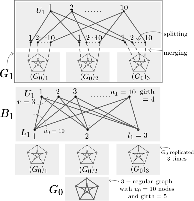
Fig. 5: Depiction of steps mentioned in the flowchart Fig 4 for an example construction of G1G_{1} for t=4t=4, r=3r=3. Here G0G_{0} is the Petersen graph. For the purpose of representation the merger of nodes is shown only for 9 nodes by the dashed lines.
Refer to caption
Fig. 6: Example of splitting a node into degree-1 nodes
Refer to caption
Fig. 7: Example of merging two nodes

The flowchart shown in Fig. 4 describes the iterative construction of the graph Gt2−1G_{\frac{t}{2}-1}. An example construction of G1G_{1} for t=4,r=3t=4,r=3 depicting the steps of the flowchart for the case of a single iteration appears in Fig. 5. We make the following observations:

  1. 1.

    For 0≤i≤t2−10\leq i\leq\frac{t}{2}-1, there are fi=∏j=i+1t2−1ljf_{i}=\prod_{j=i+1}^{\frac{t}{2}-1}l_{j} disjoint copies of GiG_{i} that reside inside Gt2−1G_{\frac{t}{2}-1} as subgraphs due to the replication steps in the construction of Gt2−1G_{\frac{t}{2}-1} (given in the flowchart Fig 4). For all t2−1>j>i\frac{t}{2}-1>j>i, since copies of GiG_{i} reside inside GjG_{j} as subgraphs, when we replicate GjG_{j} in the (j+1)t​h(j+1)^{th} replication step, all the copies of GiG_{i} contained within GjG_{j} also get replicated; we refer to all such copies of GiG_{i} here. Let us denote the disjoint union of these subgraphs corresponding to all copies of GiG_{i} formed due to replication steps by Gir​e​p=∪j=1fi(Gi)jG_{i}^{rep}=\cup_{j=1}^{f_{i}}(G_{i})_{j}, where (Gi)j(G_{i})_{j} is the jt​hj^{th} copy of GiG_{i} in Gt2−1G_{\frac{t}{2}-1} formed due to some replication step. We view Gir​e​pG_{i}^{rep} as a subgraph of Gt2−1G_{\frac{t}{2}-1}.

  2. 2.

    Note that the construction of Gt2−1G_{\frac{t}{2}-1} proceeds by adding nodes layer by layer with each layer connecting to the layer below it in a tree-like fashion while maintaining the girth of the overall graph to be atleast t+1t+1. Let N⁡(v)N(v) represent neighbors of a node vv in Gt2−1G_{\frac{t}{2}-1}. Let (Ui)j(U_{i})_{j} be the copy of UiU_{i} in V⁡((Gi)j),∀1≤j≤fiV((G_{i})_{j}),\forall 1\leq j\leq f_{i}. For 1≤i≤t2−11\leq i\leq\frac{t}{2}-1, the nodes Ti=∪j=1fi(Ui)jT_{i}=\cup_{j=1}^{f_{i}}(U_{i})_{j} represent the nodes in the it​hi^{th} layer and they connect in a tree-like fashion to the (i−1)t​h(i-1)^{th} layer nodes Ti−1=∪j=1fi−1(Ui−1)jT_{i-1}=\cup_{j=1}^{f_{i-1}}(U_{i-1})_{j}. The connection is tree-like because for v∈Tiv\in T_{i}, let Sv=N⁡(v)∩Ti−1S_{v}=N(v)\cap T_{i-1} then Sv∩Sw=∅S_{v}\cap S_{w}=\emptyset and |Sv|=|Sw|=r|S_{v}|=|S_{w}|=r ,∀v,w∈Ti,v≠w,\forall v,w\in T_{i},v\neq w and N⁡(v)∩Tp=∅,∀p∉{i−1,i+1}N(v)\cap T_{p}=\emptyset,\forall p\notin\{i-1,i+1\},∀v∈Ti\forall v\in T_{i}.

  3. 3.

    Girth of GiG_{i}: Let the girth of Gi−1G_{i-1} be at least t+1t+1. Consider the construction of graph GiG_{i} from lil_{i} replicated copies of Gi−1G_{i-1} and the biregular bipartite graph BiB_{i}. (Ui−1)j(U_{i-1})_{j} is the copy of Ui−1U_{i-1} in the jthj^{\text{th}} copy of Gi−1G_{i-1} i.e., (Gi−1)j(G_{i-1})_{j}, 1≤j≤li1\leq j\leq l_{i} appearing at the replication step in the construction of GiG_{i} from Gi−1G_{i-1}. Consider a cycle in GiG_{i}. If the cycle does not involve any nodes in UiU_{i} then it must be completely contained in (Gi−1)j(G_{i-1})_{j} for some 1≤j≤li1\leq j\leq l_{i} and hence of length at least t+1t+1 because the girth of Gi−1G_{i-1} is assumed to be at least t+1t+1. If the cycle involves a node v1∈Uiv_{1}\in U_{i} then the cycle must be of the form v1​Pa1​b1​v2​…​vq​Paq​bq​v1v_{1}P_{a_{1}b_{1}}v_{2}...v_{q}P_{a_{q}b_{q}}v_{1} (as shown in fig 8) where vm∈Ui,am,bm∈⋃j=1li(Ui−1)jv_{m}\in U_{i},a_{m},b_{m}\in\bigcup\limits_{j=1}^{l_{i}}(U_{i-1})_{j} and Pam​bmP_{a_{m}b_{m}} (shown in green in fig 8) is a path in (Gi−1)p(G_{i-1})_{p} for some 1≤p≤li1\leq p\leq l_{i} starting at ama_{m} and ending at bmb_{m} for 1≤m≤q1\leq m\leq q. This is because when we start from v1v_{1} and move to a node say a1a_{1} in ⋃j=1li(Ui−1)j\bigcup\limits_{j=1}^{l_{i}}(U_{i-1})_{j} the only way to come back to v1v_{1} for completing the cycle is by traversing a path Pa1​b1P_{a_{1}b_{1}} in (Gi−1)p(G_{i-1})_{p} for some 1≤p≤li1\leq p\leq l_{i} ending at some node b1∈(Ui−1)pb_{1}\in(U_{i-1})_{p}. By repeating the above argument it can be seen that the cycle must be of the form v1​Pa1​b1​v2​…​vq​Paq​bq​v1v_{1}P_{a_{1}b_{1}}v_{2}...v_{q}P_{a_{q}b_{q}}v_{1}. Now by above argument,for 1≤m≤q1\leq m\leq q, let am,bm∈(Ui−1)σma_{m},b_{m}\in(U_{i-1})_{\sigma_{m}}, 1≤σm≤li1\leq\sigma_{m}\leq l_{i}. Hence am,bma_{m},b_{m} must have been merged with some two nodes in VσmiV^{i}_{\sigma_{m}} (nodes coming from splitting vσmi∈Liv^{i}_{\sigma_{m}}\in L_{i} into degree 1 nodes) in the construction of GiG_{i}. Hence v1​vσ1i​v2​vσ2i​…​vq​vσqi​v1v_{1}v^{i}_{\sigma_{1}}v_{2}v^{i}_{\sigma_{2}}\ldots v_{q}v^{i}_{\sigma_{q}}v_{1} must contain a non trivial cycle in BiB_{i}. Also the length of the path Pam​bmP_{a_{m}b_{m}} is at least 2​(i−1)+12(i-1)+1 due to the tree-like structure of (Gi−1)σm(G_{i-1})_{\sigma_{m}}. Hence if the girth of BiB_{i} is gig_{i} then the length of the cycle v1​Pa1​b1​v2​…​vq​Paq​bq​v1v_{1}P_{a_{1}b_{1}}v_{2}...v_{q}P_{a_{q}b_{q}}v_{1} is at least 2​q+q⁡(2​(i−1)+1)≥gi+gi2​(2​(i−1)+1)=gi​(i+12)≥t+1i+12​(i+12)=t+12q+q(2(i-1)+1)\geq g_{i}+\frac{g_{i}}{2}(2(i-1)+1)=g_{i}(i+\frac{1}{2})\geq\frac{t+1}{i+\frac{1}{2}}(i+\frac{1}{2})=t+1. Hence girth of GiG_{i} is at least t+1t+1.

Refer to caption
Fig. 8: Figure showing a cycle in the graph GiG_{i}. Only the edges constituting a cycle are shown.

Description of a rate-optimal code 𝒞\mathcal{C} based on Gt2−1G_{\frac{t}{2}-1}:
Code 𝒞\mathcal{C} is defined on the graph Gt2−1G_{\frac{t}{2}-1} as follows:

  1. 1.

    The edges of G0r​e​pG_{0}^{rep} represent information symbols. It can be seen that the number of information symbols is k=u0​r2​∏j=1t2−1ljk=\frac{u_{0}r}{2}\prod_{j=1}^{\frac{t}{2}-1}l_{j}.

  2. 2.

    Every node of Gt2−1G_{\frac{t}{2}-1} represents a distinct parity symbol described as follows.

  3. 3.

    A node v∈V⁡(G0r​e​p)v\in V(G_{0}^{rep}) represents a parity symbol which is the binary sum of information symbols that are represented by edges in G0r​e​pG_{0}^{rep} incident on vv.

  4. 4.

    For 1≤i≤t2−11\leq i\leq\frac{t}{2}-1, a node v∈Tiv\in T_{i} in Gt2−1G_{\frac{t}{2}-1} represents a parity symbol which is the binary sum of code symbols that are represented by the nodes in N⁡(v)∩Ti−1N(v)\cap T_{i-1}.

  5. 5.

    It can be seen that the total number of nodes is n−k=∑i=0t2−1ui​∏j=i+1t2−1lj=∑i=0t2−1u0ri​∏j=1t2−1ljn-k=\sum_{i=0}^{\frac{t}{2}-1}u_{i}\prod_{j=i+1}^{\frac{t}{2}-1}l_{j}=\sum_{i=0}^{\frac{t}{2}-1}\frac{u_{0}}{r^{i}}\prod_{j=1}^{\frac{t}{2}-1}l_{j}.

  6. 6.

    𝒞\mathcal{C} is defined by the information symbols represented by edges in G0r​e​pG_{0}^{rep} and parity symbols represented by nodes in Gt2−1G_{\frac{t}{2}-1}.

  7. 7.

    From the above counts, the rate of the code 𝒞\mathcal{C} can be seen to be equal to the bound given by (1).

We now prove that 𝒞\mathcal{C} can correct tt erasures sequentially.

  1. 1.

    The Tanner graph of our code can be viewed as follows: We now view Gt2−1G_{\frac{t}{2}-1} differently to give an alternative description of our code. In the graph Gt2−1G_{\frac{t}{2}-1}, let every edge represent a code symbol and every node represent a parity check of the code symbols corresponding to the edges incident on it. Apart from this, for every node in Ut2−1(⊆V⁡(Gt2−1))U_{\frac{t}{2}-1}(\subseteq V(G_{\frac{t}{2}-1})) there is one distinct degree-1 variable node attached to it. Each of these degree-1 variable nodes corresponds to a distinct code symbol. The code symbol corresponding to a degree-1 variable node is part of the parity check represented by the node in Ut2−1U_{\frac{t}{2}-1} to which it is attached. Our code is now defined by the code symbols represented by the edges of Gt2−1G_{\frac{t}{2}-1} and degree-1 variable nodes attached to Ut2−1U_{\frac{t}{2}-1}. This completes the alternative description of our code.
    The alternative description of the code can be illustrated using the figures 9, 10 and 11.

    • •

      Consider a node v∈Tiv\in T_{i} for 1≤i≤t2−21\leq i\leq\frac{t}{2}-2 in Gt2−1G_{\frac{t}{2}-1}. In the original description of the code, the node vv represents a code symbol say cpc_{p} which is the binary sum of rr symbols say c1,c2,…,crc_{1},c_{2},...,c_{r} where c1,c2,…,crc_{1},c_{2},...,c_{r} are represented by nodes in N⁡(v)∩Ti−1N(v)\cap T_{i-1}; in the alternative description of the code the same node vv now represents the parity check cp⊕c1⊕c2⊕…⊕cr=0c_{p}\oplus c_{1}\oplus c_{2}\oplus...\oplus c_{r}=0 and as shown in figure 9 the edge going out upward from the node vv represents the code symbol cpc_{p} and the edges going out downward from vv represent the code symbols c1,c2,…,crc_{1},c_{2},...,c_{r}.

      Refer to caption
      Fig. 9: Figure showing two descriptions of our code at a node TiT_{i} for 1≤i≤t2−21\leq i\leq\frac{t}{2}-2
    • •

      Consider a node v∈Ut2−1v\in U_{\frac{t}{2}-1} in Gt2−1G_{\frac{t}{2}-1}. In the original description of the code, the node vv represents a code symbol say cpc_{p} which is the binary sum of rr symbols say c1,c2,…,crc_{1},c_{2},...,c_{r} where c1,c2,…,crc_{1},c_{2},...,c_{r} are represented by nodes in N⁡(v)∩Tt2−2N(v)\cap T_{\frac{t}{2}-2}; in the alternative description of the code the same node vv now represents the parity check cp⊕c1⊕c2⊕…⊕cr=0c_{p}\oplus c_{1}\oplus c_{2}\oplus...\oplus c_{r}=0 and as shown in figure 10 the degree-1 node attached to vv represents the code symbol cpc_{p} and the edges going out downward from vv represent the code symbols c1,c2,…,crc_{1},c_{2},...,c_{r}. Hence there is a unique distinct degree-1 node attached to every node in Ut2−1U_{\frac{t}{2}-1}. These are exactly the degree-1 variable nodes we described above in the alternative description of the code.

      Refer to caption
      Fig. 10: Figure showing two descriptions of our code at a node in Ut2−1U_{\frac{t}{2}-1}
    • •

      Consider a node v∈T0v\in T_{0} in Gt2−1G_{\frac{t}{2}-1}. In the original description of the code, the node vv represents a code symbol say cpc_{p} which is the binary sum of rr information symbols say i1,i2,…,iri_{1},i_{2},...,i_{r} where i1,i2,…,iri_{1},i_{2},...,i_{r} are represented by edges incident on vv in G0repG_{0}^{\text{rep}}; in the alternative description of the code the same node vv now represents the parity check cp⊕i1⊕i2⊕…⊕ir=0c_{p}\oplus i_{1}\oplus i_{2}\oplus...\oplus i_{r}=0 and as shown in figure 11 the edge going out upward from vv represents the code symbol cpc_{p} and the edges going out downward from vv still represents the information symbols i1,i2,…,iri_{1},i_{2},...,i_{r}.

      Refer to caption
      Fig. 11: Figure showing two descriptions of our code at a node in T0T_{0}
    • •

      We transform the meaning of nodes and edges in Gt2−1G_{\frac{t}{2}-1} from original to alternative description of the code as described above across nodes and edges of the graph Gt2−1G_{\frac{t}{2}-1} and it can be done maintaining consistency across the tranformations of meaning of nodes and edges from original to alternative description.

    • •

      By the above explanation, all the parity checks necessary to describe our code are represented by nodes in the graph Gt2−1G_{\frac{t}{2}-1} in the alternative description.

    Note that degree-1 variable nodes are not part of Gt2−1G_{\frac{t}{2}-1} and these degree-1 variable nodes are the reason for rate optimality.

  2. 2.

    Let EE be a set of erased symbols. Let the code symbols corresponding to degree-1 variable nodes be D1D_{1}. Let E∩D1=∅E\cap D_{1}=\emptyset. Let an edge (v1,v2)(v_{1},v_{2}) represent an erased symbol in EE. Construct a maximal walk P=v1​v2​…​vwP=v_{1}v_{2}...v_{w}, vi∈V⁡(Gt2−1)v_{i}\in V(G_{\frac{t}{2}-1}) ,∀i∈[w],\forall i\in[w] such that vi≠vjv_{i}\neq v_{j}, ∀w≥i≠j≥1\forall\ w\geq i\neq j\geq 1, and the edge (vi,vi+1)(v_{i},v_{i+1}) represents an erased code symbol in EE ∀i∈[w−1]\forall i\in[w-1] (walk PP is maximal in terms of number of vertices). Since the walk is maximal any edge of the form (vw,v)(v_{w},v) for v∈N⁡(vw)−{vw−1}v\in N(v_{w})-\{v_{w-1}\}, v∈V⁡(Gt2−1)v\in V(G_{\frac{t}{2}-1}):

    1. (a)

      either represents an unerased symbol for all v∈N⁡(vw)−{vw−1}v\in N(v_{w})-\{v_{w-1}\}, v∈V⁡(Gt2−1)v\in V(G_{\frac{t}{2}-1}) in which case the symbol represented by the edge (vw−1,vw)(v_{w-1},v_{w}) can be recovered by using the parity check represented by vwv_{w}.

    2. (b)

      or represents an erased symbol and v∈{v1,…,vw}v\in\{v_{1},...,v_{w}\} in which case there is a cycle. Since girth of Gt2−1G_{\frac{t}{2}-1} is ≥t+1\geq t+1, there must at least t+1t+1 distinct erased symbols.

    Hence either an erased symbol can be recovered or there are more than tt erasures. The argument can be repeated for recovering subsequent erased symbols sequentially one by one if |E|<t|E|<t.

  3. 3.

    If E∩D1≠∅E\cap D_{1}\neq\emptyset, then start with a vertex v1∈Ut2−1v_{1}\in U_{\frac{t}{2}-1} to which a degree-1 variable node corresponding to an erased code symbol is attached. Now construct a maximal walk, P=v1​…​vwP=v_{1}...v_{w}, vi∈V⁡(Gt2−1CLOSEv_{i}\in V(G_{\frac{t}{2}-1}),∀i∈[w]\forall i\in[w], on the erased symbols as before. Now either as before, one of the symbols in EE can be recovered or there are more than tt erased symbols in EE due to a cycle or the walk ends in another node in Ut2−1U_{\frac{t}{2}-1} i.e., vw∈Ut2−1v_{w}\in U_{\frac{t}{2}-1} with the code symbol corresponding to degree-1 variable node attached to vwv_{w} also being erased. Since Gt2−1G_{\frac{t}{2}-1} is tree-like, any two nodes in Ut2−1U_{\frac{t}{2}-1} are separated by a path of length at least t−1t-1 in Gt2−1G_{\frac{t}{2}-1}. Hence there are at least t−1+2=t+1t-1+2=t+1 erasures (+2 because |E∩D1|≥2|E\cap D_{1}|\geq 2).

  4. 4.

    Thus the entire point of constructing Gt2−1G_{\frac{t}{2}-1} in a tree-like fashion is for protection from more than one erasure in the code symbols corresponding to degree-1 variable nodes attached to Ut2−1U_{\frac{t}{2}-1}.

III-B Construction of codes achieving the upper bound on rate for tt odd:

In this subsection we give a construction of codes achieving the rate bound (66) for any r≥3r\geq 3 and t=2​s−1,s≥1t=2s-1,s\geq 1. A construction achieving the bound (66) for t=5t=5 can be found in [12]. For t=3t=3, the bound (66) can be achieved by taking the product of two [r+1,r][r+1,r] single parity check code (2 dimensional product code). For t=1t=1, the bound (66) can be achieved by taking the [r+1,r][r+1,r] single parity check code. Hence we give a rate optimal construction for any r≥3r\geq 3 and t=2​s−1t=2s-1, s≥2s\geq 2 in the following.
We provide an iterative, graph-based construction of rate-optimal codes for a given r≥3r\geq 3 and t=2​s−1t=2s-1, s≥2s\geq 2. We build a new graph Gs−1G_{s-1} iteratively, starting from G0G_{0} (different from the one considered for tt even case.), by adding nodes in vertical, layer-by-layer fashion. At every stage of the iteration, the graph GiG_{i} (again different from the one constructed for tt even case.) thus constructed, will always have girth ≥t+1\geq t+1. We then define our rate-optimal code based on the graph Gs−1G_{s-1}.

Construction of graph Gs−1G_{s-1}: Denote the vertex set of a graph GG by V⁡(G)V(G). We make use of graphs G0G_{0} and BiB_{i}, for 1≤i≤s−11\leq i\leq s-1 described below as the ingredients:

  1. 1.

    We pick G0G_{0} as follows: Let G0G_{0} be an rr-regular bipartite graph with girth ≥t+1\geq t+12. Let U0,1,U0,2U_{0,1},U_{0,2} be the two (upper and lower) sets of nodes in the bipartite graph with degree​(x)=r,∀x∈U0,1\text{degree}(x)=r,\forall\ x\in U_{0,1} and degree​(y)=r,∀y∈U0,2\text{degree}(y)=r,\forall\ y\in U_{0,2}. Hence V⁡(G0)=U0,1∪U0,2V(G_{0})=U_{0,1}\cup U_{0,2}. Define |U0,1|=|U0,2|=u0|U_{0,1}|=|U_{0,2}|=u_{0}.

  2. 2.

    Next, for ii in the range 1≤i≤s−11\leq i\leq s-1, we iteratively construct an (r,2​ui−1)(r,2u_{i-1})-biregular bipartite graph BiB_{i} with girth gi≥⌈t+1i+12⌉g_{i}\geq\left\lceil\frac{t+1}{i+\frac{1}{2}}\right\rceil with the following properties. Let Ui,LiU_{i},L_{i} be the two (upper and lower) sets of nodes in the bipartite graph with degree​(x)=r,∀x∈Ui\text{degree}(x)=r,\forall\ x\in U_{i} and degree​(y)=2​ui−1,∀y∈Li\text{degree}(y)=2u_{i-1},\forall\ y\in L_{i}. Hence V⁡(Bi)=Ui∪LiV(B_{i})=U_{i}\cup L_{i}. We have that Ui=Ui,1∪Ui,2U_{i}=U_{i,1}\cup U_{i,2} with |Ui,1|=|Ui,2||U_{i,1}|=|U_{i,2}| and Ui,1∩Ui,2=∅U_{i,1}\cap U_{i,2}=\emptyset. Let |Ui,1|=|Ui,2|=ui|U_{i,1}|=|U_{i,2}|=u_{i} and |Li|=li|L_{i}|=l_{i}. Therefore |Ui|=2​ui|U_{i}|=2u_{i}. By edge counting, we have 2​r​ui=2​ui−1​li2ru_{i}=2u_{i-1}l_{i} i.e. r​ui=ui−1​liru_{i}=u_{i-1}l_{i}. Additionally we have that, ∀x∈Li,|N⁡(x)∩Ui,1|=|N⁡(x)∩Ui,2|=ui−1\forall\ x\in L_{i},|N(x)\cap U_{i,1}|=|N(x)\cap U_{i,2}|=u_{i-1} where N⁡(x)N(x) denotes the neighbors of node xx in BiB_{i}. Construction of such graphs will be described separately.

Pick G0G_{0}, rr-regular bipartite graph, girth ≥(t+1)\geq(t+1), V⁡(G0)=U0,1∪U0,2V(G_{0})=U_{0,1}\cup U_{0,2}, |U0,1|=|U0,2|=u0|U_{0,1}|=|U_{0,2}|=u_{0} i=1i=1 Pick bipartite graph BiB_{i}: (r,2​ui−1)(r,2u_{i-1})-biregular, V⁡(Bi)=Ui∪LiV(B_{i})=U_{i}\cup L_{i}, Ui=Ui,1∪Ui,2U_{i}=U_{i,1}\cup U_{i,2}, girth ≥⌈(t+1)/(i+1/2)⌉\geq\left\lceil(t+1)/(i+1/2)\right\rceil, |Ui,1|=|Ui,2|=ui,|Ui|=2​ui,|Li|=li|U_{i,1}|=|U_{i,2}|=u_{i},|U_{i}|=2u_{i},\ |L_{i}|=l_{i}, ∀x∈Li,|N⁡(x)∩Ui,1|=|N⁡(x)∩Ui,2|=ui−1\forall\ x\in L_{i},\ |N(x)\cap U_{i,1}|=|N(x)\cap U_{i,2}|=u_{i-1} Let Li={v1i,v2i,…,vlii}L_{i}=\{v_{1}^{i},v_{2}^{i},...,v_{l_{i}}^{i}\} For 1≤j≤li1\leq j\leq l_{i}, split the node vji∈Liv_{j}^{i}\in L_{i} in BiB_{i} with deg​(vji)=2​ui−1\text{deg}(v_{j}^{i})=2u_{i-1}, into 2​ui−12u_{i-1} degree-1 nodes ((Vji)1∪(Vji)2)((V_{j}^{i})_{1}\cup(V_{j}^{i})_{2}) such that N⁡(vji)∩Ui,1=N⁡((Vji)1)N(v_{j}^{i})\cap U_{i,1}=N((V_{j}^{i})_{1}) and N⁡(vji)∩Ui,2=N⁡((Vji)2)N(v_{j}^{i})\cap U_{i,2}=N((V_{j}^{i})_{2}) and |(Vji)1|=|(Vji)2|=ui−1|(V_{j}^{i})_{1}|=|(V_{j}^{i})_{2}|=u_{i-1}. (Vji)1∪(Vji)2(V_{j}^{i})_{1}\cup(V_{j}^{i})_{2} is the set of 2​ui−12u_{i-1} degree-1 nodes which are formed by splitting vjiv_{j}^{i} An example of splitting a node into degree-1 nodes is shown in fig 6 Replicate the graph Gi−1G_{i-1} lil_{i} times (thus each upper node in Ui−1U_{i-1} is also replicated lil_{i} times), (Gi−1)j(G_{i-1})_{j}: jthj^{\text{th}} copy of Gi−1G_{i-1} and (Ui−1)j(U_{i-1})_{j}: copy of Ui−1U_{i-1} in (Gi−1)j(G_{i-1})_{j} (Ui−1,1)j(U_{i-1,1})_{j}: copy of Ui−1,1U_{i-1,1} in (Gi−1)j(G_{i-1})_{j} (Ui−1,2)j(U_{i-1,2})_{j}: copy of Ui−1,2U_{i-1,2} in (Gi−1)j(G_{i-1})_{j} [​Ui−1⊆V⁡(Gi−1)​]\text{[}U_{i-1}\subseteq V(G_{i-1})\text{]}

i=i+1i=i+1

Let (Ui−1,1)j={(c1(i−1,1))j,…,(cui−1(i−1,1))j}(U_{i-1,1})_{j}=\{(c_{1}^{(i-1,1)})_{j},...,(c_{u_{i-1}}^{(i-1,1)})_{j}\} (Ui−1,2)j={(c1(i−1,2))j,…,(cui−1(i−1,2))j}(U_{i-1,2})_{j}=\{(c_{1}^{(i-1,2)})_{j},...,(c_{u_{i-1}}^{(i-1,2)})_{j}\}, (Vji)1={(d1(i,1))j,…,(dui−1(i,1))j}(V_{j}^{i})_{1}=\{(d_{1}^{(i,1)})_{j},...,(d_{u_{i-1}}^{(i,1)})_{j}\} and (Vji)2={(d1(i,2))j,…,(dui−1(i,2))j}(V_{j}^{i})_{2}=\{(d_{1}^{(i,2)})_{j},...,(d_{u_{i-1}}^{(i,2)})_{j}\} Merge the node (cm(i−1,p))j∈(Ui−1,p)j(c_{m}^{(i-1,p)})_{j}\in(U_{i-1,p})_{j} with (dm(i,p))j∈(Vji)p(d_{m}^{(i,p)})_{j}\in(V_{j}^{i})_{p}, ∀ 1≤m≤ui−1\forall\ 1\leq m\leq u_{i-1}, ∀ 1≤p≤2\forall\ 1\leq p\leq 2 and ∀ 1≤j≤li\forall\ 1\leq j\leq l_{i} An example of merging two nodes is shown in fig 7 The resulting graph is GiG_{i}; it can be verified that GiG_{i} has girth ≥t+1\geq t+1, the nodes Ui⊂V⁡(Gi)U_{i}\subset V(G_{i}) now form the upper layer of the graph GiG_{i} and these are the nodes in GiG_{i} that participate in the next iterative step is i=s−1​?i=s-1?stopNOYES
Fig. 12: Flowchart showing the iterative construction of Gs−1G_{s-1}.

Construction of BiB_{i}:

  • •

    Consider a (r,ui−1)(r,u_{i-1})-biregular bipartite graph G1=(X1∪X2,E)G^{1}=(X_{1}\cup X_{2},E) with girth at least ⌈t+1i+12⌉\left\lceil\frac{t+1}{i+\frac{1}{2}}\right\rceil. Let X1={b1,…,bm^}X_{1}=\{b_{1},...,b_{\hat{m}}\}, X2={c1,…,cλ}X_{2}=\{c_{1},...,c_{\lambda}\} for some m^,λ\hat{m},\lambda with degree​(bj)=r\text{degree}(b_{j})=r, for 1≤j≤m^1\leq j\leq\hat{m} and degree​(cj)=ui−1\text{degree}(c_{j})=u_{i-1}, for 1≤j≤λ1\leq j\leq\lambda. Such a graph G1G^{1} can be constructed due to [20].

  • •

    Consider a λ\lambda-regular bipartite graph G2=(X∪Y,E)G^{2}=(X\cup Y,E) with girth at least 12​⌈t+1i+12⌉\frac{1}{2}\left\lceil\frac{t+1}{i+\frac{1}{2}}\right\rceil. Let X={x1,…,xl′}X=\{x_{1},...,x_{l^{\prime}}\} and Y={y1,…,yl′}Y=\{y_{1},...,y_{l^{\prime}}\} for some l′l^{\prime} with each node of degree λ\lambda. Such a graph G2G^{2} can be constructed due to [20].

  • •

    Take 2​l′2l^{\prime} disjoint copies of G1G^{1}. Let G3G^{3} be the disjoint union of the 2​l′2l^{\prime} copies named G11,…,G2​l′1G^{1}_{1},...,G^{1}_{2l^{\prime}} of G1G^{1}. Denote the nodes bj,cjb_{j},c_{j} in the lt​hl^{th} copy Gl1G^{1}_{l} by bjl,cjlb^{l}_{j},c^{l}_{j} respectively.

  • •

    Replace the node xfx_{f} in G2G^{2} by the nodes x1,f,…,xλ,fx_{1,f},...,x_{\lambda,f} for 1≤f≤l′1\leq f\leq l^{\prime}. If the neighbors of xfx_{f} in G2G^{2} are the nodes in the set {yq1,…,yqλ}\{y_{q_{1}},...,y_{q_{\lambda}}\} then connect xj,fx_{j,f} to yqjy_{q_{j}} for 1≤j≤λ1\leq j\leq\lambda. Now replace the node yfy_{f} by the nodes y1,f,…,yλ,fy_{1,f},...,y_{\lambda,f} for 1≤f≤l′1\leq f\leq l^{\prime}. If the neighbors of yfy_{f} after replacing the nodes in XX were the nodes in the set {xσ1,β1,…,xσλ,βλ}\{x_{\sigma_{1},\beta_{1}},...,x_{\sigma_{\lambda},\beta_{\lambda}}\} then connect yj,fy_{j,f} to xσj,βjx_{\sigma_{j},\beta_{j}} for 1≤j≤λ1\leq j\leq\lambda. Denote this graph by G4G^{4}. For every edge (xj,f,yj^,f^)(x_{j,f},y_{\hat{j},\hat{f}}) in G4G^{4} merge the nodes cjfc^{f}_{j} and cj^l′+f^c^{l^{\prime}+\hat{f}}_{\hat{j}} in G3G^{3} and label the resulting merged node as v(f−1)​λ+jiv^{i}_{(f-1)\lambda+j} in G3G^{3}. Relabel bjlb^{l}_{j} as c(l−1)​m^+j(i,1)c^{(i,1)}_{(l-1)\hat{m}+j}, ∀1≤l≤l′\forall 1\leq l\leq l^{\prime},∀1≤j≤m^\forall 1\leq j\leq\hat{m} in G3G^{3}. Relabel bjlb^{l}_{j} as c(l−l′−1)​m^+j(i,2)c^{(i,2)}_{(l-l^{\prime}-1)\hat{m}+j}, ∀l′+1≤l≤2​l′\forall\ l^{\prime}+1\leq l\leq 2l^{\prime},∀1≤j≤m^\forall 1\leq j\leq\hat{m} in G3G^{3} . After the merging and relabeling of nodes in G3G^{3} as described, resulting graph is named as BiB_{i}.

  • •

    The constructed graph BiB_{i} is a (r,2​ui−1)(r,2u_{i-1})-biregular bipartite graph Bi=(Ui∪Li,Ei)B_{i}=(U_{i}\cup L_{i},E_{i}) with Ui=Ui,1∪Ui,2U_{i}=U_{i,1}\cup U_{i,2} where Ui,1={c1(i,1),…,cui(i,1)}U_{i,1}=\{c_{1}^{(i,1)},...,c_{u_{i}}^{(i,1)}\}, Ui,2={c1(i,2),…,cui(i,2)}U_{i,2}=\{c_{1}^{(i,2)},...,c_{u_{i}}^{(i,2)}\} and ui=l′​m^u_{i}=l^{\prime}\hat{m} and Li={v1i,…,vlii}L_{i}=\{v^{i}_{1},...,v^{i}_{l_{i}}\} where li=l′​λl_{i}=l^{\prime}\lambda and degree​(cj(i,p))=r\text{degree}(c_{j}^{(i,p)})=r for 1≤j≤ui1\leq j\leq u_{i},1≤p≤21\leq p\leq 2 and degree​(vji)=2​ui−1\text{degree}(v^{i}_{j})=2u_{i-1} for 1≤j≤li1\leq j\leq l_{i}. It can be seen that BiB_{i} has girth at least ⌈t+1i+12⌉\left\lceil\frac{t+1}{i+\frac{1}{2}}\right\rceil. It can also be seen from the construction of BiB_{i} that |N⁡(vji)∩Ui,1|=|N⁡(vji)∩Ui,2|=ui−1|N(v^{i}_{j})\cap U_{i,1}|=|N(v^{i}_{j})\cap U_{i,2}|=u_{i-1}, for 1≤j≤li1\leq j\leq l_{i}.

Construction of Gs−1G_{s-1}: The flowchart shown in Fig. 12 describes the iterative construction of the graph Gs−1G_{s-1}.

We make the following observations (similar observations compared to tt even case):

  1. 1.

    For 0≤i≤s−10\leq i\leq s-1, there are fi=∏j=i+1s−1ljf_{i}=\prod_{j=i+1}^{s-1}l_{j} disjoint copies of GiG_{i} that reside inside Gs−1G_{s-1} as subgraphs due to the replication steps in the construction of Gs−1G_{s-1} (given in the flowchart Fig 12). For all s−1>j>is-1>j>i, since copies of GiG_{i} reside inside GjG_{j} as subgraphs, when we replicate GjG_{j} in the (j+1)t​h(j+1)^{th} replication step, all the copies of GiG_{i} contained within GjG_{j} also get replicated; we refer to all such copies of GiG_{i} here. Let us denote the disjoint union of these subgraphs corresponding to all copies of GiG_{i} formed due to replication steps by Gir​e​p=∪j=1fi(Gi)jG_{i}^{rep}=\cup_{j=1}^{f_{i}}(G_{i})_{j}, where (Gi)j(G_{i})_{j} is the jt​hj^{th} copy of GiG_{i} in Gs−1G_{s-1} formed due to some replication step. We view Gir​e​pG_{i}^{rep} as a subgraph of Gs−1G_{s-1}.

  2. 2.

    Note that the construction of Gs−1G_{s-1} proceeds by adding nodes layer by layer with each layer connecting to the layer below it in a tree-like fashion while maintaining the girth of overall graph to be atleast t+1t+1. Let N⁡(v)N(v) represent neighbors of a node vv in Gs−1G_{s-1}. Let (Ui)j(U_{i})_{j} be the copy of UiU_{i} in V⁡((Gi)j),∀1≤j≤fiV((G_{i})_{j}),\forall 1\leq j\leq f_{i}. For 1≤i≤s−11\leq i\leq s-1, the nodes Ti=∪j=1fi(Ui)jT_{i}=\cup_{j=1}^{f_{i}}(U_{i})_{j} represent the nodes in the it​hi^{th} layer and they connect in a tree-like fashion to the (i−1)t​h(i-1)^{th} layer nodes Ti−1=∪j=1fi−1(Ui−1)jT_{i-1}=\cup_{j=1}^{f_{i-1}}(U_{i-1})_{j}. The connection is tree-like because for v∈Tiv\in T_{i}, let Sv=N⁡(v)∩Ti−1S_{v}=N(v)\cap T_{i-1} then Sv∩Sw=∅S_{v}\cap S_{w}=\emptyset and |Sv|=|Sw|=r|S_{v}|=|S_{w}|=r ,∀v,w∈Ti,v≠w,\forall v,w\in T_{i},v\neq w and N⁡(v)∩Tp=∅,∀p∉{i−1,i+1}N(v)\cap T_{p}=\emptyset,\forall p\notin\{i-1,i+1\},∀v∈Ti\forall v\in T_{i}.

  3. 3.

    For 1≤p≤21\leq p\leq 2, let (Ui,p)j(U_{i,p})_{j} be the copy of Ui,pU_{i,p} in V⁡((Gi)j),∀1≤j≤fiV((G_{i})_{j}),\forall 1\leq j\leq f_{i}. In fact it can be seen that for 1≤i≤s−11\leq i\leq s-1, the nodes in Tip=∪j=1fi(Ui,p)jT^{p}_{i}=\cup_{j=1}^{f_{i}}(U_{i,p})_{j} connect in a tree-like fashion to nodes in Ti−1p=∪j=1fi(Ui−1,p)jT^{p}_{i-1}=\cup_{j=1}^{f_{i}}(U_{i-1,p})_{j} for p∈{1,2}p\in\{1,2\}. The connection is tree-like because for v∈Tipv\in T^{p}_{i}, let Svp=N⁡(v)∩Ti−1pS^{p}_{v}=N(v)\cap T^{p}_{i-1} then Svp∩Swp=∅S^{p}_{v}\cap S^{p}_{w}=\emptyset and |Svp|=|Swp|=r|S^{p}_{v}|=|S^{p}_{w}|=r ,∀v,w∈Tpi,v≠w,\forall v,w\in T^{p}_{i},v\neq w and N⁡(v)∩Tqp=∅,∀q∉{i−1,i+1}N(v)\cap T^{p}_{q}=\emptyset,\forall q\notin\{i-1,i+1\},∀v∈Tip\forall v\in T^{p}_{i}. This implies a tree-like graph is built starting from bottom layer T0pT^{p}_{0} (leaf-like nodes) towards Ts−1pT^{p}_{s-1}. It can seen that the tree-like graph built from T01T^{1}_{0} does not intersect or disjoint with tree-like graph built from T02T^{2}_{0}. The only interaction between these 2 tree-like graphs is by edges representing information symbols connecting nodes in T01T^{1}_{0} with T02T^{2}_{0}.

  4. 4.

    The fact that GiG_{i} has girth at least t+1t+1 can be proved using arguments similar to those used in tt even case. Hence we skip the proof.

Description of a rate-optimal code 𝒞\mathcal{C} based on Gs−1G_{s-1}:
Code 𝒞\mathcal{C} is defined on the graph Gs−1G_{s-1}. We will first describe a code 𝒞1\mathcal{C}_{1} based on Gs−1G_{s-1}. On puncturing the code 𝒞1\mathcal{C}_{1} by dropping few parity symbols, we get our desired rate-optimal code 𝒞\mathcal{C}.
Code 𝒞1\mathcal{C}_{1} is defined on the graph Gs−1G_{s-1} as follows:

  1. 1.

    The edges of G0r​e​pG_{0}^{rep} represent information symbols. It can be seen that the number of information symbols is k=u0​r​∏j=1s−1ljk=u_{0}r\prod_{j=1}^{s-1}l_{j}.

  2. 2.

    Every node of Gs−1G_{s-1} represents a distinct parity symbol described as follows.

  3. 3.

    A node v∈V⁡(G0r​e​p)v\in V(G_{0}^{rep}) represents a parity symbol which is the binary sum of information symbols that are represented by edges in G0r​e​pG_{0}^{rep} incident on vv.

  4. 4.

    For 1≤i≤s−11\leq i\leq s-1, a node v∈Tiv\in T_{i} in Gs−1G_{s-1} represents a parity symbol which is the binary sum of code symbols that are represented by the nodes in N⁡(v)∩Ti−1N(v)\cap T_{i-1}.

  5. 5.

    It can be seen that the total number of nodes is n′−k=∑i=0s−12​ui​∏j=i+1s−1lj=2​∑i=0s−1u0ri​∏j=1s−1ljn^{\prime}-k=\sum_{i=0}^{s-1}2u_{i}\prod_{j=i+1}^{s-1}l_{j}=2\sum_{i=0}^{s-1}\frac{u_{0}}{r^{i}}\prod_{j=1}^{s-1}l_{j}.

  6. 6.

    𝒞1\mathcal{C}_{1} is an [n′,k][n^{\prime},k] code defined by the information symbols represented by edges in G0r​e​pG_{0}^{rep} and parity symbols represented by nodes in Gs−1G_{s-1}.

Code 𝒞\mathcal{C} is defined as follows:

  1. 1.

    Puncture the code 𝒞1\mathcal{C}_{1} by dropping the parity symbols represented by nodes in Us−1,2U_{s-1,2}. Hence 𝒞\mathcal{C} is an [n,k][n,k] code defined by the information symbols represented by edges in G0r​e​pG_{0}^{rep} and parity symbols represented by nodes in V⁡(Gs−1)−Us−1,2V(G_{s-1})-U_{s-1,2}.

  2. 2.

    Hence n−k=n′−k−us−1=2​∑i=0s−2ui​∏j=i+1s−1lj+us−1=2​∑i=0s−2u0ri​∏j=1s−1lj+u0rs−1​∏j=1s−1ljn-k=n^{\prime}-k-u_{s-1}=2\sum_{i=0}^{s-2}u_{i}\prod_{j=i+1}^{s-1}l_{j}+u_{s-1}=2\sum_{i=0}^{s-2}\frac{u_{0}}{r^{i}}\prod_{j=1}^{s-1}l_{j}+\frac{u_{0}}{r^{s-1}}\prod_{j=1}^{s-1}l_{j}.

  3. 3.

    From the above counts, the rate of the code 𝒞\mathcal{C} can be seen to be equal to the bound given by (66).

The proof that 𝒞\mathcal{C} can correct tt erasures sequentially is similar to the tt even case. Hence we skip the proof but we give the main idea as follows. The only point to be noted for sequential recovery of tt erasures considering the cases we have dealt with in tt even case is that nodes in the top most layer which are part of the code 𝒞\mathcal{C} i.e., nodes in Ts−11∪Ts−22T^{1}_{s-1}\cup T^{2}_{s-2} are separated from each other with just enough distance that a path of erased symbols connecting any two nodes (representing erased symbols) at this top-most layer (similar to tt even case) must have at least t+1t+1 erased symbols. Since the path between 2 nodes in Ts−22T^{2}_{s-2} is potentially smaller than the the path between two nodes in Ts−11T^{1}_{s-1}, we need a little extra distance separating two nodes in Ts−22T^{2}_{s-2} which is given by the bipartite nature of the graph at bottom most layer since the path from a node in Ts−22T^{2}_{s-2} can reach another node in Ts−22T^{2}_{s-2} only through two nodes T02T^{2}_{0} we get 1 extra distance as any two nodes in T02T^{2}_{0} is separated by a distance of atleast 2 due to the bipartite nature of G0r​e​pG_{0}^{rep}. This is precisely the reason why we built tree-like graph from T01T^{1}_{0} disjointly from T02T^{2}_{0}, so that when we puncture which drops the distance between nodes in top most layer, we get a little extra distance at the bottom layer.

Remark 4.

The following conjecture on the rate of an (n,k,r,t)s​e​q(n,k,r,t)_{seq} code appeared in [13].

kn≤11+∑i=1mairi,\displaystyle\frac{k}{n}\leq\frac{1}{1+\sum_{i=1}^{m}\frac{a_{i}}{r^{i}}},
ai≥0,ai∈ℤ,∑i=1mai=t,\displaystyle a_{i}\geq 0,a_{i}\in\mathbb{Z},\sum_{i=1}^{m}a_{i}=t,
m=⌈l​o​gr​(k)⌉.\displaystyle m=\lceil log_{r}(k)\rceil.

Our rate bound verifies the conjecture as our rate bound can be written in the form:

For tt even:

kn≤11+∑i=1t22ri.\displaystyle\frac{k}{n}\leq\frac{1}{1+\sum_{i=1}^{\frac{t}{2}}\frac{2}{r^{i}}}.

For tt Odd:

kn≤11+∑i=1s−12ri+1rs.\displaystyle\frac{k}{n}\leq\frac{1}{1+\sum_{i=1}^{s-1}\frac{2}{r^{i}}+\frac{1}{r^{s}}}.

More specific conjecture was given for t=5,6t=5,6. While our bound proves the conjecture for t=5t=5, the conjectured upper bound for t=6t=6 does not hold as our upper bound on code rate is both larger and achievable).

For t=6t=6, Our bound takes the form:

kn≤r3r3+2​r2+2​r+2\displaystyle\frac{k}{n}\leq\frac{r^{3}}{r^{3}+2r^{2}+2r+2}
kn≤11+2r+2r2+2r3\displaystyle\frac{k}{n}\leq\frac{1}{1+\frac{2}{r}+\frac{2}{r^{2}}+\frac{2}{r^{3}}}

The conjecture for t=6t=6 given in [13]:

kn≤11+2r+3r2+1r3\displaystyle\frac{k}{n}\leq\frac{1}{1+\frac{2}{r}+\frac{3}{r^{2}}+\frac{1}{r^{3}}}

Hence the conjecture given in [13] has a smaller rate than our bound for t=6t=6. And further our upper bound on rate for t=6t=6 can be achieved.

Remark 5.

In [9] the authors provide a construction of a code with sequential recovery for any rr and tt having rate r−1r+1+1n\frac{r-1}{r+1}+\frac{1}{n}. r−1r+1+1n\frac{r-1}{r+1}+\frac{1}{n} will meet our rate bound exactly when a Moore graph of degree r+1r+1 and girth t+1t+1 exists. Moore graphs(degree = r+1r+1, girth = t+1t+1) are shown to not exist for any t∉{2,3,4,5,7,11}t\notin\{2,3,4,5,7,11\} for any r≥2r\geq 2 (see [21]). Hence the construction in [9] is not rate-optimal for most of the cases.

Appendix A Proof of Claim 1

It is enough to show that:

  • •

    {Ai}\{A_{i}\} are matrices with each column having Hamming weight 1.

  • •

    {Di}\{D_{i}\} are matrices with each row having Hamming weight 1.

As the point 1 written above combined with the fact that each column of [AiDi]\left[\frac{A_{i}}{D_{i}}\right] has Hamming weight 2 implies Di,i≥1D_{i},i\geq 1 are matrices with each column having Hamming weight 1 and D0D_{0} by definition is a matrix with each column having Hamming weight 1.
Let us denote the jthj^{\text{th}} column of matrix H1H_{1} by h¯j\underline{h}_{j}, 1≤j≤n1\leq j\leq n. Let us show the claim by induction as follows:
(Note that in the arguments that follow h¯p1,…,h¯pψ\underline{h}_{p_{1}},...,\underline{h}_{p_{\psi}}, h¯y1,…,h¯yϕ\underline{h}_{y_{1}},...,\underline{h}_{y_{\phi}}, h¯z1,…,h¯zθ\underline{h}_{z_{1}},...,\underline{h}_{z_{\theta}} and h¯w1,…,h¯wγ\underline{h}_{w_{1}},...,\underline{h}_{w_{\gamma}} will be repeatedly used each time denoting some set of column vectors not necessarily related to a different instance of the same notation.)

Induction Hypothesis:

  • •

    Property PiP_{i}: any m×1m\times 1 vector having Hamming weight at most 2 with support contained in {∑l=0i−1ρl+1,..,∑l=0i−1ρl+ρi}\{\sum_{l=0}^{i-1}\rho_{l}+1,..,\sum_{l=0}^{i-1}\rho_{l}+\rho_{i}\} can be written as some linear combination of at most 2​(i+1)2(i+1) column vectors of H1H_{1} say h¯p1,…,h¯pψ\underline{h}_{p_{1}},...,\underline{h}_{p_{\psi}} for some {p1,…,pψ}⊆{1,…,∑l=0ial}\{p_{1},...,p_{\psi}\}\subseteq\{1,...,\sum_{l=0}^{i}a_{l}\} and 0<ψ≤2​(i+1)0<\psi\leq 2(i+1).

  • •

    Let us assume as induction hypthesis that the property PiP_{i} is true and the Claim 1 is true for A1,…​AiA_{1},...A_{i}, D0,…​DiD_{0},...D_{i}.

Initial step:

  • •

    We show that each row of D0D_{0} has Hamming weight exactly 1.
    Suppose there exists a row of D0D_{0} with Hamming weight more than 1; let the support set of the row be {i1,i2,…}\{i_{1},i_{2},...\}. Then the columns h¯i1,h¯i2\underline{h}_{i_{1}},\underline{h}_{i_{2}} of H1H_{1} can be linearly combined to give a zero column. This contradicts the fact that dm​i​n​(𝒞)≥t+1,t>0d_{min}({\mathcal{C}})\geq t+1,t>0 and tt is even. Hence, all rows of D0D_{0} have Hamming weight exactly 1.

  • •

    If t=2t=2, then the claim is already proved. So let t≥4t\geq 4.

  • •

    We show that each column of A1A_{1} has Hamming weight exactly 1.
    Suppose jt​hj^{th} column of A1A_{1} for some ​1≤j≤a1\text{for some }1\leq j\leq a_{1} has Hamming weight 2; let the support of the column be {j1,j2}\{j_{1},j_{2}\} in A1A_{1}. Then the column h¯a0+j\underline{h}_{a_{0}+j} in H1H_{1} along with the 2 column vectors of H1H_{1} say h¯p1,h¯p2\underline{h}_{p_{1}},\underline{h}_{p_{2}} where {p1,p2}⊆{1,…,a0}\{p_{1},p_{2}\}\subseteq\{1,...,a_{0}\} where h¯p1\underline{h}_{p_{1}} has exactly one non-zero entry in j1t​hj_{1}^{th} co-ordinate and h¯p2\underline{h}_{p_{2}} has exactly one non-zero entry j2t​hj_{2}^{th} co-ordinate, can be linearly combined to give a zero column again leading to a contradiction on minimum distance. Such columns with one column having only one non-zero entry exactly in j1t​hj_{1}^{th} co-ordinate and another column having only one non-zero entry exactly in j2t​hj_{2}^{th} co-ordinate with column labels in {1,…,a0}\{1,...,a_{0}\} exist due to the single weight columns in the matrix D0D_{0}.

  • •

    The above argument also shows that any m×1m\times 1 vector having Hamming weight at most 2 with support contained in {1,..,ρ0}\{1,..,\rho_{0}\} can be written as some linear combination of at most 2 column vectors of H1H_{1} say h¯p1,…,h¯pψ\underline{h}_{p_{1}},...,\underline{h}_{p_{\psi}} for some {p1,…,pψ}⊆{1,…,a0}\{p_{1},...,p_{\psi}\}\subseteq\{1,...,a_{0}\} (ψ=1​ or ​2\psi=1\text{ or }2). Hence Property P0P_{0} is true.

  • •

    We now show that each row of D1D_{1} has Hamming weight exactly 1. Suppose jt​hj^{th} row of D1D_{1} has Hamming weight more than 1; let the support set of the row be {l1,l2,…,lz}\{l_{1},l_{2},...,l_{z}\} in D1D_{1}. Now there is some linear combination of columns h¯a0+l1\underline{h}_{a_{0}+l_{1}} and h¯a0+l2\underline{h}_{a_{0}+l_{2}} in H1H_{1} that gives a zero in (ρ0+j)t​h(\rho_{0}+j)^{th} co-ordinate and thus this linear combination has support contained in {1,…,ρ0}\{1,...,\rho_{0}\} with Hamming weight at most 2. Now applying Property P0P_{0} on this linear combination implies that there is a non-empty set of at most 44 linearly dependent columns in H1H_{1} leading to a contradiction on minimum distance.

  • •

    Now we show that Property P1P_{1} is true: We have to prove that any m×1m\times 1 vector with Hamming weight at most 22 with support contained in {ρ0+1,..,ρ0+ρ1}\{\rho_{0}+1,..,\rho_{0}+\rho_{1}\} can be written as linear combination of at most 2​(1+1)=42(1+1)=4 column vectors of H1H_{1} say h¯p1,…,h¯pψ\underline{h}_{p_{1}},...,\underline{h}_{p_{\psi}} for some {p1,…,pψ}⊆{1,…,∑l=01al}\{p_{1},...,p_{\psi}\}\subseteq\{1,...,\sum_{l=0}^{1}a_{l}\} and 0<ψ≤40<\psi\leq 4. This can be easily seen using arguments similar to ones presented before. Let an m×1m\times 1 vector have non-zero entries exactly in co-ordinates ρ0+j1,ρ0+j2\rho_{0}+j_{1},\rho_{0}+j_{2} or ρ0+j1\rho_{0}+j_{1}. Then this vector can be linearly combined with at most 2 column vectors in H1H_{1} say h¯y1,…,h¯yϕ\underline{h}_{y_{1}},...,\underline{h}_{y_{\phi}} where {y1,…,yϕ}⊆{a0+1,…,a0+a1}\{y_{1},...,y_{\phi}\}\subseteq\{a_{0}+1,...,a_{0}+a_{1}\} (ϕ=1​ or ​2\phi=1\text{ or }2) (2 columns h¯y1,h¯y2\underline{h}_{y_{1}},\underline{h}_{y_{2}} with first and second column having a non-zero entry in co-ordinates ρ0+j1,ρ0+j2\rho_{0}+j_{1},\rho_{0}+j_{2} respectively or a column h¯y1\underline{h}_{y_{1}} with a non-zero entry in (ρ0+j1)t​h(\rho_{0}+j_{1})^{th} co-ordinate. These columns h¯y1,h¯y2\underline{h}_{y_{1}},\underline{h}_{y_{2}} or h¯y1\underline{h}_{y_{1}} exist due to D1D_{1}.) to form a m×1m\times 1 vector with Hamming weight at most 2 with support contained in {1,…,ρ0}\{1,...,\rho_{0}\} which in turn can be written as linear combination of at most 22 column vectors in H1H_{1} say h¯z1,…,h¯zθ\underline{h}_{z_{1}},...,\underline{h}_{z_{\theta}} for some {z1,…,zθ}⊆{1,…,a0}\{z_{1},...,z_{\theta}\}\subseteq\{1,...,a_{0}\} (θ=1\theta=1 or 22) by property P0P_{0}. Hence the given m×1m\times 1 vector is written as linear combination of at most 2​(1+1)=42(1+1)=4 column vectors in H1H_{1} say h¯w1,…,h¯wγ\underline{h}_{w_{1}},...,\underline{h}_{w_{\gamma}} for some {w1,…,wγ}⊆{1,…,∑l=01al}\{w_{1},...,w_{\gamma}\}\subseteq\{1,...,\sum_{l=0}^{1}a_{l}\} and 0<γ≤40<\gamma\leq 4.

Induction step :

  • •

    Let us assume by induction hypothesis that Property PiP_{i} is true and the Claim 1 is true for A1,…​AiA_{1},...A_{i}, D0,…​DiD_{0},...D_{i} for some i≤t2−2i\leq\frac{t}{2}-2 and prove the induction hypothesis for i+1i+1. For t=4t=4, the initial step of induction completes the proof of Claim 1. Hence assume t>4t>4.

  • •

    Now we show that each column of Ai+1A_{i+1} has Hamming weight exactly 1: suppose jt​hj^{th} column of Ai+1A_{i+1} for some 1≤j≤ai+11\leq j\leq a_{i+1} has Hamming weight 2; let the support of the column be j1,j2j_{1},j_{2} in Ai+1A_{i+1}. It is clear that the corresponding column vector h¯∑l=0ial+j\underline{h}_{\sum\limits_{l=0}^{i}a_{l}+j} in H1H_{1} is a vector with support contained in {∑l=0i−1ρl+1,..,∑l=0i−1ρl+ρi}\{\sum_{l=0}^{i-1}\rho_{l}+1,..,\sum_{l=0}^{i-1}\rho_{l}+\rho_{i}\} and Hamming weight 2. Now applying Property PiP_{i} on this column vector h¯∑l=0ial+j\underline{h}_{\sum\limits_{l=0}^{i}a_{l}+j} implies that there is a non-empty set of at most 2​(i+1)+12(i+1)+1 columns in H1H_{1} which are linearly dependent; hence contradicts the minimum distance as 2​(i+1)+1≤t−12(i+1)+1\leq t-1. Hence each column of Ai+1A_{i+1} has Hamming weight exactly 1.

  • •

    Now we show that each row of Di+1D_{i+1} has Hamming weight exactly 1: suppose jt​hj^{th} row of Di+1D_{i+1} has Hamming weight more than 1; let the support set of the row be {l1,…,lz}\{l_{1},...,l_{z}\} in Di+1D_{i+1}. Now some linear combination of columns h¯∑j=0iaj+l1\underline{h}_{\sum\limits_{j=0}^{i}a_{j}+l_{1}} and h¯∑j=0iaj+l2\underline{h}_{\sum\limits_{j=0}^{i}a_{j}+l_{2}} in H1H_{1} will make the resulting vector have a 00 in (∑l=0iρl+j)t​h(\sum\limits_{l=0}^{i}\rho_{l}+j)^{th} co-ordinate and the resulting vector also has Hamming weight at most 2 with support contained in {∑l=0i−1ρl+1,..,∑l=0i−1ρl+ρi}\{\sum_{l=0}^{i-1}\rho_{l}+1,..,\sum_{l=0}^{i-1}\rho_{l}+\rho_{i}\} and hence applying Property PiP_{i} on this resulting vector implies that there is a non-empty set of at most 2​(i+1)+22(i+1)+2 columns in H1H_{1} which are linearly dependent; hence contradicts the minimum distance as 2​(i+1)+2≤t2(i+1)+2\leq t; thus proving that each row of Di+1D_{i+1} has Hamming weight exactly 1.

  • •

    Now we show that Property Pi+1P_{i+1} is true: We have to prove that any m×1m\times 1 vector with Hamming weight at most 22 with support contained in {∑l=0iρl+1,..,∑l=0iρl+ρi+1}\{\sum_{l=0}^{i}\rho_{l}+1,..,\sum_{l=0}^{i}\rho_{l}+\rho_{i+1}\} can be written as linear combination of at most 2​(i+2)2(i+2) column vectors of H1H_{1} say h¯p1,…,h¯pψ\underline{h}_{p_{1}},...,\underline{h}_{p_{\psi}} for some {p1,…,pψ}⊆{1,…,∑l=0i+1al}\{p_{1},...,p_{\psi}\}\subseteq\{1,...,\sum_{l=0}^{i+1}a_{l}\} and 0<ψ≤2​(i+2)0<\psi\leq 2(i+2). This can be easily seen using arguments similar to ones presented before. Let an m×1m\times 1 vector have non-zero entries in co-ordinates ∑l=0iρl+j1,∑l=0iρl+j2\sum_{l=0}^{i}\rho_{l}+j_{1},\sum_{l=0}^{i}\rho_{l}+j_{2} or ∑l=0iρl+j1\sum_{l=0}^{i}\rho_{l}+j_{1}. Then this vector can be linearly combined with at most 2 column vectors in H1H_{1} say h¯y1,…,h¯yϕ\underline{h}_{y_{1}},...,\underline{h}_{y_{\phi}} where {y1,…,yϕ}⊆{∑l=0ial+1,…,∑l=0ial+ai+1}\{y_{1},...,y_{\phi}\}\subseteq\{\sum_{l=0}^{i}a_{l}+1,...,\sum_{l=0}^{i}a_{l}+a_{i+1}\} with ϕ=1\phi=1 or 22, (2 columns h¯y1,h¯y2\underline{h}_{y_{1}},\underline{h}_{y_{2}} with first column and second column having a non-zero entry in co-ordinates ∑l=0iρl+j1,∑l=0iρl+j2\sum_{l=0}^{i}\rho_{l}+j_{1},\sum_{l=0}^{i}\rho_{l}+j_{2} respectively or a column h¯y1\underline{h}_{y_{1}} with a non-zero entry in (∑l=0iρl+j1)t​h(\sum_{l=0}^{i}\rho_{l}+j_{1})^{th} co-ordinate. These columns h¯y1,h¯y2\underline{h}_{y_{1}},\underline{h}_{y_{2}} or h¯y1\underline{h}_{y_{1}} exist due to Di+1D_{i+1}.) to form a m×1m\times 1 vector with Hamming weight at most 2 with support contained in {∑l=0i−1ρl+1,∑l=0i−1ρl+ρi}\{\sum_{l=0}^{i-1}\rho_{l}+1,\sum_{l=0}^{i-1}\rho_{l}+\rho_{i}\} which in turn can be written as linear combination of at most 2​(i+1)2(i+1) column vectors in H1H_{1} say h¯z1,…,h¯zθ\underline{h}_{z_{1}},...,\underline{h}_{z_{\theta}} for some {z1,…,zθ}⊆{1,…,∑l=0ial}\{z_{1},...,z_{\theta}\}\subseteq\{1,...,\sum_{l=0}^{i}a_{l}\} and 0<θ≤2​(i+1)0<\theta\leq 2(i+1) by property PiP_{i}. Hence the given m×1m\times 1 vector is written as linear combination of at most 2​(i+2)2(i+2) column vectors in H1H_{1} say h¯w1,…,h¯wγ\underline{h}_{w_{1}},...,\underline{h}_{w_{\gamma}} for some {w1,…,wγ}⊆{1,…,∑l=0i+1al}\{w_{1},...,w_{\gamma}\}\subseteq\{1,...,\sum_{l=0}^{i+1}a_{l}\} and 0<γ≤2​(i+2)0<\gamma\leq 2(i+2).

References

  • [1] S. B. Balaji, K. P. Prasanth, and P. V. Kumar, “Binary codes with locality for multiple erasures having short block length,” CoRR, 2016. [Online]. Available: http://arxiv.org/abs/1601.07122/
  • [2] P. Gopalan, C. Huang, H. Simitci, and S. Yekhanin, “On the Locality of Codeword Symbols,” IEEE Trans. Inf. Theory, vol. 58, no. 11, pp. 6925–6934, Nov. 2012.
  • [3] D. Papailiopoulos and A. Dimakis, “Locally repairable codes,” in Information Theory Proceedings (ISIT), 2012 IEEE International Symposium on, July 2012, pp. 2771–2775.
  • [4] F. Oggier and A. Datta, “Self-repairing homomorphic codes for distributed storage systems,” in INFOCOM, 2011 Proceedings IEEE, April 2011, pp. 1215–1223.
  • [5] C. Huang, M. Chen, and J. Li, “Pyramid codes: Flexible schemes to trade space for access efficiency in reliable data storage systems,” in Network Computing and Applications, 2007. NCA 2007. Sixth IEEE International Symposium on, July 2007, pp. 79–86.
  • [6] G. Kamath, N. Prakash, V. Lalitha, and P. Kumar, “Codes with local regeneration,” in Information Theory and Applications Workshop (ITA), 2013, Feb 2013, pp. 1–5.
  • [7] I. Tamo and A. Barg, “A family of optimal locally recoverable codes,” IEEE Trans. Inf. Theory, vol. 60, no. 8, pp. 4661–4676, 2014.
  • [8] N. Prakash, V. Lalitha, and P. V. Kumar, “Codes with locality for two erasures,” CoRR, vol. abs/1401.2422, 2014. [Online]. Available: http://arxiv.org/abs/1401.2422
  • [9] A. Rawat, A. Mazumdar, and S. Vishwanath, “On cooperative local repair in distributed storage,” in Information Sciences and Systems (CISS), 2014 48th Annual Conference on, 2014, pp. 1–5.
  • [10] W. Song and C. Yuen, “Locally repairable codes with functional repair and multiple erasure tolerance,” CoRR, vol. abs/1507.02796, 2015. [Online]. Available: http://arxiv.org/abs/1507.02796
  • [11] ——, “Binary locally repairable codes - sequential repair for multiple erasures,” CoRR, vol. abs/1511.06034, 2015. [Online]. Available: http://arxiv.org/abs/1511.06034
  • [12] S. Balaji, K. Prasanth, and P. V. Kumar, “Binary codes with locality for four erasures,” arXiv preprint arXiv:1607.02817, 2016.
  • [13] W. Song, K. Cai, and C. Yuen, “On sequential locally repairable codes,” arXiv preprint arXiv:1610.09767, 2016.
  • [14] N. Prakash, G. Kamath, V. Lalitha, and P. Kumar, “Optimal linear codes with a local-error-correction property,” in Proc. IEEE Int. Symp. Inf. Theory (ISIT), 2012, pp. 2776–2780.
  • [15] W. Song, S. H. Dau, C. Yuen, and T. Li, “Optimal locally repairable linear codes,” Selected Areas in Communications, IEEE Journal on, vol. 32, no. 5, pp. 1019–1036, May 2014.
  • [16] I. Tamo, A. Barg, and A. Frolov, “Bounds on the parameters of locally recoverable codes,” CoRR, vol. abs/1506.07196, 2015. [Online]. Available: http://arxiv.org/abs/1506.07196
  • [17] A. Wang and Z. Zhang, “Repair locality from a combinatorial perspective,” in Proc. IEEE Int. Symp. Inf. Theory (ISIT), 2014, pp. 1972–1976.
  • [18] ——, “Repair locality with multiple erasure tolerance,” IEEE Trans. Inf. Theory, vol. 60, no. 11, pp. 6979–6987, 2014.
  • [19] L. Pamies-Juarez, H. Hollmann, and F. Oggier, “Locally repairable codes with multiple repair alternatives,” in Information Theory Proceedings (ISIT), 2013 IEEE International Symposium on, July 2013, pp. 892–896.
  • [20] Z. Furedi, F. Lazebnik, A. Seress, V. A. Ustimenko, and A. J. Woldar, “Graphs of prescribed girth and bi-degree,” Journal of Combinatorial Theory Ser. B 64 (2), pp. 228–239, 1995.
  • [21] G. Exoo and R. Jajcay, “Dynamic cage survey,” Electron. J. Combin, Dynamic Survey, 2013.