On the critical probability in percolation

Svante Janson ^†^†thanks: Department of Mathematics, Uppsala University, PO Box 480, SE-751˜06 Uppsala, Sweden. E-mail: svante.janson@math.uu.se. Part of the work was done during visits to the University of Cambridge and to the Isaac Newton Institute for Mathematical Sciences during the programme Theoretical Foundations for Statistical Network Analysis (EPSCR Grant Number EP/K032208/1) and was partially supported by a grant from the Knut and Alice Wallenberg Foundation and a grant from the Simons foundation. Lutz Warnke ^†^†thanks: Department of Pure Mathematics and Mathematical Statistics, University of Cambridge, Wilberforce Road, Cambridge CB3 0WB, UK; and School of Mathematics, Georgia Institute of Technology, Atlanta GA˜30332, USA. E-mail: L.Warnke@dpmms.cam.ac.uk. Part of the work was done while interning with the Theory Group at Microsoft Research, Redmond; LW thanks Yuval Peres for introducing him to the topic of this paper.

November 25, 2016

Abstract

For percolation on finite transitive graphs, Nachmias and Peres suggested a characterization of the critical probability based on the logarithmic derivative of the susceptibility. As a first test-case, we study their suggestion for the Erdős–Rényi random graph $G_{n,p}$ , and confirm that the logarithmic derivative has the desired properties: (i) its maximizer lies inside the critical window $p=1/n+\Theta(n^{-4/3})$ , and (ii) the inverse of its maximum value coincides with the $\Theta(n^{-4/3})$ –width of the critical window. We also prove that the maximizer is not located at $p=1/n$ or $p=1/(n-1)$ , refuting a speculation of Peres.

1 Introduction

The percolation phase transition on finite graphs is one of the most intriguing and striking phenomena at the intersection of mathematical physics, combinatorics, and probability theory. The classical Erdős–Rényi random graph $G_{n,p}$ is perhaps the most carefully studied reference model: as the edge probability $p$ increases past the ‘critical probability’ $p_{c}=1/n$ , the global structure changes radically, from only small components to a single giant component plus small ones. More precisely, using the parametrization $p=1/n+\lambda_{n}n^{-4/3}$ , and for simplicity assuming $p=\Theta(1/n)$ , by the inspiring work of Erdős and Rényi [11], Bollobás [4], Łuczak [27], and Aldous [3], we nowadays distinguish three qualitatively different phases of $G_{n,p}$ . In the subcritical phase $\lambda_{n}\to-\infty$ , the $r=\Theta(1)$ largest components $C_{1},\ldots,C_{r}$ are typically all of comparable size: $|C_{1}|\sim|C_{2}|\sim\cdots\sim|C_{r}|=\Theta(n^{2/3}\lambda_{n}^{-2}\log|\lambda_{n}|)=o(n^{2/3})$ . In the supercritical phase $\lambda_{n}\to\infty$ , the largest component typically dominates all other components: $|C_{2}|\ll|C_{1}|=\Theta(\lambda_{n}n^{2/3})$ . In the critical window $|\lambda_{n}|=O(1)$ , the rescaled sizes $|C_{1}|/n^{2/3},|C_{2}|/n^{2/3},\cdots$ of the largest components converge in distribution to non-degenerate random variables, i.e., they are not concentrated.

In the language of mathematical physics, $G_{n,p}$ interpreted as percolation on the complete $n$ -vertex graph is a mean-field model. Hence, we expect that the percolation phase transition of many ‘high dimensional’ finite graphs is similar, with the hypercube and various tori being examples of great interest (see, e.g., [2, 5, 18, 7, 8, 9, 16]). To fix notation, we assume that $G$ is a given transitive $n$ -vertex graph, and we write $G_{p}\subseteq G$ for the binomial random subgraph where each edge is included independently with probability $p$ . As pointed out by Nachmias and Peres [29], in this general percolation setting it is a challenging problem to find a good definition of the critical probability $p_{c}$ , such that for a suitable critical window around $p_{c}$ , for example, the size of the largest component is not concentrated.

The folklore average degree heuristic $p_{c}=1/(\mathrm{deg}_{G}(v)-1)$ is a natural first guess (the graph $G$ is assumed to be transitive and thus regular, so the choice of the vertex $v$ does not matter). For the hypercube with vertex set $\{0,1\}^{m}$ , and thus degree $m$ , Ajtai, Komlós and Szemerédi [2] showed that there is a critical threshold $(1+o(1))/m$ ; this was sharpened by Bollobás, Kohayakawa, and Łuczak [5], who raised the question whether the critical probability might be exactly $1/(m-1)$ . However, Borgs, Chayes, van der Hofstad, Slade and Spencer [7, 8] and van der Hofstad and Nachmias [16, 17] have shown that there is critical window of width $\Theta(n^{-1/3}p_{c})=\Theta(2^{-m/3}/m)$ about a critical probability $p_{c}$ , which by van der Hofstad and Slade [18] satisfies $p_{c}=1/(m-1)+3.5m^{-3}+O(m^{-4})$ ; since the width of the window is $o(m^{-3})$ , the value $1/(m-1)$ is outside the critical window.

A more sophisticated suggestion for the critical probability was pioneered by Borgs, Chayes, van der Hofstad, Slade and Spencer [7, 8] (and used for the hypercube result just described). They essentially proposed to define $p_{c}=p_{c}(G)$ as the unique solution to the polynomial equation

(1.1)

\raisebox{2.0pt}{$\chi$}_{G}(p):={\mathbb{E}}_{p}|C(v)|=n^{1/3},

where the susceptibility $\raisebox{2.0pt}{$\chi$}_{G}(p)$ denotes the expected size of the component $C(v)$ containing a fixed vertex $v$ in $G_{p}$ . (This is a widely studied key parameter in percolation theory and random graph theory, see, e.g., [1, 13, 22, 25, 32, 33]. Since $G$ is assumed to be transitive, the choice of $v$ does not matter.) The aforementioned technical definition is guided by Erdős–Rényi mean-field type behaviour. Indeed, in the subcritical phase we expect that $C(v)$ closely mimics a subcritical branching process, which suggests that typically $|C_{1}|\approx(\raisebox{2.0pt}{$\chi$}_{G}(p))^{2}$ up to logarithmic corrections (see, e.g., Section 1.2 in [15] or Proposition 5.1 in [1]). Furthermore, in the supercritical phase we expect that the largest component dominates all other components, which by transitivity suggests that $\raisebox{2.0pt}{$\chi$}_{G}(p)\approx{\mathbb{E}}_{p}|C_{1}|^{2}/n$ . Assuming that inside the critical window we can observe subcritical and supercritical features, it thus seems plausible that the critical probability should roughly satisfy $\raisebox{2.0pt}{$\chi$}_{G}(p)\approx{\mathbb{E}}_{p}|C_{1}|^{2}/n\approx\raisebox{2.0pt}{$\chi$}_{G}(p)^{4}/n$ , motivating the choice of equation (1.1). Borgs et al. [7, 8] showed that (a minor variant of) the discussed definition is very useful in combination with the so-called finite triangle condition: they recovered many Erdős–Rényi features under such generic mean-field assumptions (see [16, 17] for some more recent developments).

As pointed out by Peres [31], the suggestion of Borgs et al. [7, 8] builds the mean-field scaling $\Theta(n^{1/3})$ into the definition of the critical probability. It would be desirable to have a useful general definition that recovers this scaling for $n$ -vertex mean-field graphs $G=G_{n}$ , rather than having separate definitions for each different scaling behaviour (or, in mathematical physics jargon, for each ‘universality class’). With this aim in mind, Nachmias and Peres [29] suggested to define $p_{c}=p_{c}(G)$ as the value of $p$ which maximizes the logarithmic derivative

(1.2)

\frac{\mathrm{d}}{\mathrm{d}p}\log\raisebox{2.0pt}{$\chi$}_{G}(p)=\frac{\frac{\mathrm{d}}{\mathrm{d}p}{\mathbb{E}}_{p}|C(v)|}{{\mathbb{E}}_{p}|C(v)|}.

To motivate this definition, note that by the Margulis–Russo formula [28, 34] the derivative $\frac{\mathrm{d}}{\mathrm{d}p}{\mathbb{E}}_{p}|C(v)|$ intuitively counts the expected (weighted) number of edges of $G_{p}$ which can affect the size of $|C(v)|$ , see also Section 2. In other words, $p_{c}$ equals the probability where the addition of a random edge has maximum relative impact on the component size $|C(v)|$ . Denoting the maximum value of (1.2) by $M=M(G)$ , Warnke [36] conjectured that for mean-field graphs $G$ the width of the critical window is of order $\Theta(1/M)$ . This is motivated by the fact that $\log(\raisebox{2.0pt}{$\chi$}_{G}(p_{2})/\raisebox{2.0pt}{$\chi$}_{G}(p_{1}))=\int_{p_{1}}^{p_{2}}\frac{\mathrm{d}}{\mathrm{d}p}\log\raisebox{2.0pt}{$\chi$}_{G}(p)dp\leqslant(p_{2}-p_{1})M$ entails that the susceptibility satisfies $\raisebox{2.0pt}{$\chi$}_{G}(p_{2})=\Theta(\raisebox{2.0pt}{$\chi$}_{G}(p_{1}))$ for $p_{2}-p_{1}=O(1/M)$ .

1.1 Main results

In this paper we investigate, as a first test-case, the suggested definition of Nachmias and Peres [29] for the Erdős–Rényi random graph $G_{n,p}$ i.e., the case $G=K_{n}$ (as proposed by Peres [31]). Here our first main result confirms that their definition of the critical probability $p_{c}$ has the desired properties, i.e., that for $G_{n,p}=(K_{n})_{p}$ the logarithmic derivative $\frac{\mathrm{d}}{\mathrm{d}p}\log\raisebox{2.0pt}{$\chi$}_{K_{n}}(p)$ satisfies the following:

(i)

its maximizer lies inside the critical window $p=1/n+O(n^{-4/3})$ , and
(ii)

the inverse of its maximum value coincides with the $\Theta(n^{-4/3})$ –width of the critical window.

Theorem 1.1 (Maximizer of the logarithmic derivative for $G_{n,p}$ ).

We have

(1.3)		$\displaystyle\biggl\|\argmax_{p\in(0,1)}\frac{\mathrm{d}}{\mathrm{d}p}\log\raisebox{2.0pt}{$\chi$}_{K_{n}}(p)-\frac{1}{n}\biggr\|=O(n^{-4/3}),$
(1.4)		$\displaystyle\max_{p\in(0,1)}\frac{\mathrm{d}}{\mathrm{d}p}\log\raisebox{2.0pt}{$\chi$}_{K_{n}}(p)=\Theta(n^{4/3}).$

Remark 1.2.

Theorem 1.3 shows that (1.3) remains valid with $O(n^{-4/3})$ replaced by $\Theta(n^{-4/3})$ .

Having established the qualitative behaviour of the logarithmic derivative for $G_{n,p}$ , it is intriguing to investigate the finer scaling behaviour inside critical window. By symmetry considerations it might be tempting to believe that $p=1/n$ or $p=1/(n-1)$ could be the maximizer of $\frac{\mathrm{d}}{\mathrm{d}p}\log\raisebox{2.0pt}{$\chi$}_{K_{n}}(p)$ , as speculated by Peres [31]. Our second main result refutes this tantalizing belief, instead strengthening the general feeling that $\lambda=0$ is no special point inside the critical window of form $p=1/n+\lambda n^{-4/3}$ .

Theorem 1.3 (Scaling inside the critical window of $G_{n,p}$ ).

Given $\lambda\in{\mathbb{R}}$ , for $p=1/n+\bigl(\lambda+o(1)\bigr)n^{-4/3}$ we have, as $n\to\infty$ ,

(1.5)		$\displaystyle\frac{\raisebox{2.0pt}{$\chi$}_{K_{n}}(p)}{n^{1/3}}$	$\displaystyle\to f(\lambda),$
(1.6)		$\displaystyle\frac{\frac{\mathrm{d}}{\mathrm{d}p}\log\raisebox{2.0pt}{$\chi$}_{K_{n}}(p)}{n^{4/3}}$	$\displaystyle\to\frac{\mathrm{d}}{\mathrm{d}\lambda}\log f(\lambda)>0,$

where the infinitely differentiable function $f=f_{2}:{\mathbb{R}}\to(0,\infty)$ is defined in (3.1)–(3.4). Moreover, if $p=1/n+\lambda n^{-4/3}$ , then the convergence in (1.5)–(1.6) is uniform for $\lambda$ in any compact interval $[\lambda_{1},\lambda_{2}]\subset{\mathbb{R}}$ . Furthermore,

(1.7)

\frac{\mathrm{d}^{2}}{\mathrm{d}\lambda^{2}}\log f(0)\neq 0.

The definition of the function $f$ appearing in Theorem 1.3 is quite involved, since it intuitively needs to capture the contribution of components with arbitrary numbers of cycles. It is easy to find asymptotics as $\lambda\to\pm\infty$ ; we have $f(\lambda)\sim|\lambda|^{-1}$ as $\lambda\to-\infty$ and $f(\lambda)\sim 4\lambda^{2}$ as $\lambda\to+\infty$ ; hence $\log f(\lambda)=-\log|\lambda|+o(1)$ as $\lambda\to-\infty$ and $\log f(\lambda)=2\log\lambda+O(1)$ as $\lambda\to+\infty$ ; furthermore, $\frac{\mathrm{d}}{\mathrm{d}\lambda}\log f(\lambda)=O(1/|\lambda|)$ for all $\lambda\in\mathbb{R}$ , see Appendix A for proofs. Theorem 1.3 also extends to convergence of higher derivatives, see Appendix C.

It would be interesting to know whether the logarithmic derivative $\frac{\mathrm{d}}{\mathrm{d}\lambda}\log f(\lambda)$ has a unique maximizer $\lambda^{*}$ , and whether it is unimodal. Figure 1 below (which is obtained by numerical integrations) suggests that this is the case, with $\lambda^{*}\approx 1$ (we conjecture $\lambda^{*}>1$ based on our limited precision numerical data).

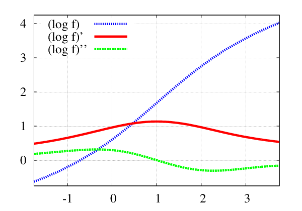
Refer to caption — Figure 1: Plot of the functions $\log f(\lambda)$ , $\frac{\mathrm{d}}{\mathrm{d}\lambda}\log f(\lambda)$ and $\frac{\mathrm{d}^{2}}{\mathrm{d}\lambda^{2}}\log f(\lambda)$ for $\lambda\in[-1.75,3.75]$ , where $f$ is as in Theorem 1.3. It provides some evidence for our belief that $\frac{\mathrm{d}}{\mathrm{d}\lambda}\log f(\lambda)$ has a unique maximizer $\lambda^{*}\approx 1$ .

The high-level structure of our proofs is as follows. For Theorem 1.1 our starting point is the Margulis–Russo Formula, which allows us to write $\frac{\mathrm{d}}{\mathrm{d}p}\raisebox{2.0pt}{$\chi$}_{K_{n}}(p)$ in terms of sums involving the squared component sizes of $G_{n,p}$ . Using ideas from random graph theory we then estimate these sums, combining correlation inequalities and the ‘symmetry rule’ (also called ‘discrete duality principle’) with results for the largest component and the susceptibility of $G_{n,p}$ , which eventually implies (1.3)–(1.4); see Section 2. For Theorem 1.3 with $p=1/n+\bigl(\lambda+o(1)\bigr)n^{-4/3}$ , our starting point is the well-known fact that $X_{n,2}=\sum_{j\geqslant 1}|C_{j}|^{2}/n^{4/3}\overset{\mathrm{d}}{\to}W_{\lambda,2}$ for some random variable $W_{\lambda,2}$ . Using technical arguments we then justify taking expectations and derivatives, which in view of $\raisebox{2.0pt}{$\chi$}_{K_{n}}(p)/n^{1/3}={\mathbb{E}}_{p}X_{n,2}$ eventually establishes (1.5)–(1.6) with $f(\lambda)={\mathbb{E}}W_{\lambda,2}$ ; see Section 3.1. For inequality (1.7) we show that $f$ and its derivatives can be computed at $\lambda=0$ by series expansions (exploiting recursive formulas for the area under a normalized Brownian excursion). Since these series converge exponentially, we can then numerically verify (1.7) by finite truncation; see Section 3.2.

1.2 Remarks on some other graphs

In the present paper we discuss only the Erdős–Rényi random graph $G_{n,p}=(K_{n})_{p}$ , i.e., percolation on the complete $n$ -vertex graph. In particular, Theorem 1.1 shows that the definition of the critical probability $p_{c}$ suggested by Nachmias and Peres [29, 31] ‘works’ in this case. It is an interesting open problem to establish analogous results for other finite graphs.

For example, consider again the hypercube with vertex set $\{0,1\}^{m}$ discussed above, see [7, 8, 16, 17]. In the subcritical phase $p=(1-\varepsilon)p_{c}$ with $\varepsilon^{3}n\to\infty$ , [7, Proposition A.1] combined with [8, Theorem 1.3 and Theorem 1.5] show that $\frac{\mathrm{d}}{\mathrm{d}p}\raisebox{2.0pt}{$\chi$}_{G}(p)\sim m(\raisebox{2.0pt}{$\chi$}_{G}(p))^{2}$ and $\raisebox{2.0pt}{$\chi$}_{G}(p)\sim\varepsilon^{-1}$ , and thus

\frac{\mathrm{d}}{\mathrm{d}p}\log\raisebox{2.0pt}{$\chi$}_{G}(p)\sim m\raisebox{2.0pt}{$\chi$}_{G}(p)=\Theta(\varepsilon^{-1}m)=o\bigl(n^{1/3}m\bigr).

In the supercritical phase $p=(1+\varepsilon)p_{c}$ with $\varepsilon^{3}n\to\infty$ and $\varepsilon=\varepsilon(n)\to 0$ , we have $\raisebox{2.0pt}{$\chi$}_{G}(p)\sim 4\varepsilon^{2}n$ according to [16, Theorem 1.1]; hence it is natural to conjecture that the logarithmic derivative satisfies

\frac{\mathrm{d}}{\mathrm{d}p}\log\raisebox{2.0pt}{$\chi$}_{G}(p)=p_{c}^{-1}\frac{\mathrm{d}}{\mathrm{d}\varepsilon}\log\raisebox{2.0pt}{$\chi$}_{G}(p)\approx\frac{2}{\varepsilon p_{c}}=\Theta(\varepsilon^{-1}m)=o\bigl(n^{1/3}m\bigr),

in the supercritical phase too, and, moreover, that the logarithmic derivative has a maximum of order $\Theta(n^{1/3}m)$ which is attained inside the critical window. Proving this, however, remains a challenging problem.

Another important example would be random $d$ -regular graphs with $d=d(n)\to\infty$ .

Moreover, it would be conceptually very interesting to start with the maximizer of (1.2) and then derive properties of the phase transition of $G_{p}$ (rather than, as in this paper, using known results for $G_{p}$ to verify properties of the maximizer).

It also seems highly desirable to better understand the critical probability $p_{c}$ for finite transitive graphs $G$ which do not exhibit the mean-field behavior of the complete graph $K_{n}$ or the hypercube $\{0,1\}^{m}$ . Here the perhaps simplest example is percolation on the $n$ -vertex cycle, $n\geqslant 3$ , for which it is not difficult to check that there are three different phases: (i) for $1-p=o(n^{-1})$ we typically have $|C_{1}|=n$ , (ii) for $1-p=\omega(n^{-1})$ we typically have $|C_{1}|=o(n)$ , and (iii) for $1-p=\Theta(n^{-1})$ the rescaled sizes $|C_{1}|/n,\cdots,|C_{r}|/n$ of the $r=\Theta(1)$ largest components are not concentrated. Hence the critical window is parametrized by $p=1-\lambda_{n}n^{-1}$ with $\lambda_{n}=\Theta(1)$ . For $p\in(0,1)$ it is routine to see that

	$\displaystyle{\mathbb{E}}_{p}\|C(v)\|$	$\displaystyle=1+\sum_{1\leqslant j<n}(p^{j}+p^{n-j}-p^{n})=1+\sum_{1\leqslant j<n}(2p^{j}-p^{n}),$
	$\displaystyle\frac{\mathrm{d}}{\mathrm{d}p}{\mathbb{E}}_{p}\|C(v)\|$	$\displaystyle=\sum_{1\leqslant j<n}(2jp^{j-1}-np^{n-1})=\sum_{1\leqslant j<n}2jp^{j-1}(1-p^{n-j}).$

A short calculation shows that ${\mathbb{E}}_{p}|C(v)|=\Theta(n^{1/3})$ implies $p=1-\Theta(n^{-1/3})$ . Furthermore, $\frac{\mathrm{d}}{\mathrm{d}p}\log{\mathbb{E}}_{p}|C(v)|=\Theta(n)$ for $1-p=\Theta(n^{-1})$ , and $\frac{\mathrm{d}}{\mathrm{d}p}\log{\mathbb{E}}_{p}|C(v)|=\Theta(\min\{(1-p)n^{2},(1-p)^{-1}\})=o(n)$ otherwise. For the critical probability $p_{c}$ of $n$ -vertex cycles, it follows that the mean-field definition of Borgs et al. fails (as expected, since cycles are not ‘high dimensional’). By contrast, the definition based on the maximizer of the logarithmic derivative of the susceptibility does correctly predict $p_{c}=1-\Theta(n^{-1})$ and the $\Theta(n^{-1})$ –width of the critical window, supporting the hope that this definition might work beyond the mean-field case.

1.3 Some notation

For emphasis, we will often use ${\mathbb{P}}_{n,p}$ and ${\mathbb{E}}_{n,p}$ for probability and expectation with respect to $G_{n,p}$ . We let $C_{i}$ denote the components of $G_{n,p}$ in order of decreasing sizes, $|C_{1}|\geqslant|C_{2}|\geqslant\cdots$ (resolving ties by taking the component with the smallest vertex label first, for definiteness). Finally, convergence in distribution is denoted $\overset{\mathrm{d}}{\to}$ , and unspecified limits are as $n\to\infty$ .

2 Maximizer of the logarithmic derivative

In this section we prove Theorem 1.1. Our arguments combine the Margulis–Russo formula with results and ideas from random graph theory. For mathematical convenience we shall work with the ‘rescaled’ susceptibility parameters

(2.1)

\displaystyle S(G_{n,p})

\displaystyle:=\sum_{v\in[n]}|C(v)|=\sum_{i}|C_{i}|^{2},

where the component $C(v)$ is with respect to $G_{n,p}$ , as usual, and

(2.2)

\displaystyle S_{n}(p)

\displaystyle:={\mathbb{E}}S(G_{n,p})={\mathbb{E}}_{n,p}\Bigl(\sum_{i}|C_{i}|^{2}\Bigr).

Recall that $\raisebox{2.0pt}{$\chi$}_{K_{n}}(p):={\mathbb{E}}_{n,p}|C(v)|$ , which is the same for every $v\in[n]$ by symmetry, and thus by (2.1)–(2.2)

(2.3)

\displaystyle S_{n}(p)

\displaystyle=n\raisebox{2.0pt}{$\chi$}_{K_{n}}(p),

which implies

(2.4)

\displaystyle\frac{\mathrm{d}}{\mathrm{d}p}\log\raisebox{2.0pt}{$\chi$}_{K_{n}}(p)=\frac{\mathrm{d}}{\mathrm{d}p}\log S_{n}(p).

Theorem 1.1 follows from equation (2.4) and inequalities (2.5)–(2.6) of Theorem 2.1 below. (In fact, in the lower bound (2.6), it suffices to consider, for example, $\lambda=0$ .)

Theorem 2.1 (Bounds for the logarithmic derivative).

There is a constant $C>0$ such that, for all $n\geqslant 1$ and $p\in(0,1)$ ,

(2.5)

\frac{\mathrm{d}}{\mathrm{d}p}\log S_{n}(p)\leqslant C\cdot\min\bigl\{|p-1/n|^{-1},\>n^{4/3}\bigr\}.

Furthermore, for every $\lambda\in{\mathbb{R}}$ there is a constant $D_{\lambda}>0$ such that, for all $n\geqslant 2$ and $p=1/n+\lambda n^{-4/3}\in(0,1)$ ,

(2.6)

\frac{\mathrm{d}}{\mathrm{d}p}\log S_{n}(p)\geqslant D_{\lambda}n^{4/3}.

The remainder of this section is devoted to the proof of Theorem 2.1, and we start by studying a combinatorial form of $\frac{\mathrm{d}}{\mathrm{d}p}S_{n}(p)$ . Writing $v\leftrightarrow w$ for the event that $v$ and $w$ are connected (which trivially holds if $v=w$ ), note that $S(G)=\sum_{v,w\in V(G)}\mathbbm{1}_{{\{{v\leftrightarrow w}\}}}$ and thus, by taking the expectation, see (2.2),

(2.7)

S_{n}(p)=\sum_{v,w\in[n]}{\mathbb{P}}_{n,p}(v\leftrightarrow w).

We now record the following simple monotonicity property, which is obvious from (2.7).

Lemma 2.2.

If $p\leqslant p^{\prime}$ and $n\leqslant n^{\prime}$ , then $S_{n}(p)\leqslant S_{n^{\prime}}(p^{\prime})$ . ∎

We say that an edge $e\in E(K_{n})$ is pivotal for $v\leftrightarrow w$ , if $v\leftrightarrow w$ in $G_{n,p}+e$ and $v\not\leftrightarrow w$ in $G_{n,p}-e$ (i.e., in the possibly modified graphs where $e$ is added and removed, respectively). Recalling the form of (2.7), for $p\in(0,1)$ the Margulis–Russo Formula [28, 34] gives

(2.8)

\frac{\mathrm{d}}{\mathrm{d}p}S_{n}(p)=\sum_{v,w\in[n]}\frac{\mathrm{d}}{\mathrm{d}p}{\mathbb{P}}_{n,p}(v\leftrightarrow w)=\sum_{v,w\in[n]}\sum_{e\in E(K_{n})}{\mathbb{P}}_{n,p}(\text{$e$ is pivotal for $v\leftrightarrow w$}).

Let ${\mathcal{P}}_{e,v,w}$ denote the event that (i) $e\not\in G_{n,p}$ and (ii) $e$ is pivotal for $v\leftrightarrow w$ . Since being pivotal does not depend on the status of $e$ , it follows that

(2.9)

\frac{\mathrm{d}}{\mathrm{d}p}S_{n}(p)=\frac{{\mathbb{E}}_{n,p}\bigl(\sum_{v,w\in[n]}\sum_{e\in E(K_{n})}\mathbbm{1}_{{\{{{\mathcal{P}}_{e,v,w}}\}}}\bigr)}{1-p}.

An edge not present in $G_{n,p}$ is pivotal for $v\leftrightarrow w$ if and only if one of its endpoints is in $C(v)$ and the other is in $C(w)\neq C(v)$ . Hence $\sum_{e\in E(K_{n})}\mathbbm{1}_{{\{{{\mathcal{P}}_{e,v,w}}\}}}=\mathbbm{1}_{{\{{C(v)\neq C(w)}\}}}|C(v)||C(w)|$ . Consequently,

(2.10)

\sum_{v,w\in[n]}\sum_{e\in E(K_{n})}\mathbbm{1}_{{\{{{\mathcal{P}}_{e,v,w}}\}}}=\sum_{v\in[n]}|C(v)|\sum_{w\not\in C(v)}|C(w)|=\sum_{i\neq j}|C_{i}|^{2}|C_{j}|^{2},

and thus, by (2.9),

(2.11)

\frac{\mathrm{d}}{\mathrm{d}p}S_{n}(p)=\frac{{\mathbb{E}}_{n,p}\left(\sum_{v\in[n]}|C(v)|\sum_{w\not\in C(v)}|C(w)|\right)}{1-p}=\frac{{\mathbb{E}}_{n,p}\left(\sum_{i\neq j}|C_{i}|^{2}|C_{j}|^{2}\right)}{1-p},

which eventually allows us to bring random graph theory into play.

2.1 Upper bounds

In this subsection we prove the upper bound (2.5) from Theorem 2.1.

We shall use some more or less well-known results for the susceptibility and the size of the largest component of $G_{n,p}$ in near-critical cases, which we state as the following theorem. (See, e.g., [7, 22, 25, 6] for similar or related results.)

Theorem 2.3.

(i)

There is a constant $D>0$ such that, for all $n\geqslant 1$ , $p\in[0,1]$ , and $\varepsilon>0$ ,

(2.12)		$\displaystyle S_{n}(p)$	$\displaystyle\leqslant\varepsilon^{-1}n\qquad$		$\displaystyle\text{if $np\leqslant 1-\varepsilon$},$
(2.13)		$\displaystyle S_{n}(p)$	$\displaystyle\leqslant D\varepsilon^{2}n^{2}\qquad$		$\displaystyle\text{if $np\leqslant 1+\varepsilon$ and $\varepsilon^{3}n\geqslant 1$}.$

(ii)

For any $A>0$ there are constants $a,B,n_{0}>0$ such that, for all $n\geqslant n_{0}$ , $p\in[0,1]$ , $\varepsilon\in(0,A]$ , and $\delta\in(0,1/2]$ satisfying $np=1+\varepsilon$ and $\delta^{2}\varepsilon^{3}n\geqslant B$ ,

(2.14)

{\mathbb{P}}_{n,p}\bigl(\bigl||C_{1}|-\rho(\varepsilon)n\bigr|\geqslant\delta\rho(\varepsilon)n\bigr)\leqslant e^{-a\delta^{2}\varepsilon^{3}n},

where $\rho(\varepsilon)>0$ is the positive solution to $1-\rho(\varepsilon)=e^{-(1+\varepsilon)\rho(\varepsilon)}$ .

(iii)

Furthermore, for any $A>0$ there are constants $\delta\in(0,1/2)$ and $c>0$ such that, for all $\varepsilon\in(0,A]$ ,

(2.15) $0<\bigl(1-(1-\delta)\rho(\varepsilon)\bigr)\cdot(1+\varepsilon)\leqslant 1-c\varepsilon.$

Proof.

The subcritical upper bound (2.12) for the susceptibility is simple and well-known. The supercritical upper bound (2.13) is intuitively clear, since in the supercritical range, the susceptibility ought to be dominated by ${\mathbb{E}}_{n,p}|C_{1}|^{2}$ and $|C_{1}|$ is with high probability $\Theta(n\varepsilon)$ when $np=1+\varepsilon$ . However, we are unaware of a reference which contains a short proof of (2.13), and thus for completeness we give in Appendix B proofs of both upper bounds (2.12)–(2.13) for the susceptibility.

The tail bound (2.14) follows from [6, Theorem 4, (10) and Remark 3].

The estimate (2.15) follows for small $\varepsilon$ , say $\varepsilon\leqslant\varepsilon_{0}$ , from the fact that $\rho(\varepsilon)=2\varepsilon+o(\varepsilon)$ as $\varepsilon\to 0$ , and for $\varepsilon\in[\varepsilon_{0},A]$ from the fact that (with $\rho=\rho(\varepsilon)$ ) $(1-\rho)(1+\varepsilon)=-(1-\rho)\log(1-\rho)/\rho<1$ for $\varepsilon>0$ together with the continuity of $\rho(\varepsilon)$ . (Cf. e.g. [22, Lemma A.2].) ∎

Corollary 2.4.

There are constants $n_{0},\pi_{0},b>0$ such that, for all $n\geqslant n_{0}$ and $p\in[0,1]$ satisfying $np\geqslant\pi_{0}$ , we have ${\mathbb{P}}(|C_{1}|\leqslant n/2)\leqslant e^{-bn}$ and $S_{n}(p)\geqslant n^{2}/8$ .

Proof.

Choose $\varepsilon$ such that $\rho(\varepsilon)\geqslant 3/4$ and let $\pi_{0}:=1+\varepsilon$ . Then the tail estimate (2.14) and monotonicity yield ${\mathbb{P}}_{n,p}(|C_{1}|\leqslant n/2)\leqslant{\mathbb{P}}_{n,\pi_{0}/n}(|C_{1}|\leqslant n/2)\leqslant e^{-bn}$ . The second conclusion follows from $S_{n}(p)\geqslant{\mathbb{E}}|C_{1}|^{2}\geqslant(n/2)^{2}{\mathbb{P}}(|C_{1}|\geqslant n/2)$ . ∎

We next prove two convenient auxiliary estimates.

Lemma 2.5.

For all $n\geqslant 1$ and $p\in[0,1]$ ,

(2.16)		$\displaystyle{\mathbb{E}}_{n,p}\Bigl(\sum_{i\neq j}\|C_{i}\|^{2}\|C_{j}\|^{2}\Bigr)$	$\displaystyle\leqslant S_{n}(p)^{2}=\Bigl({\mathbb{E}}_{n,p}\bigl(\sum_{i}\|C_{i}\|^{2}\bigr)\Bigr)^{2},$
(2.17)		$\displaystyle{\mathbb{E}}_{n,p}\Bigl(\sum_{i,j}\|C_{i}\|^{2}\|C_{j}\|^{2}\Bigr)$	$\displaystyle\leqslant\Bigl(S_{n}(p)+3\bigl[n^{-1}S_{n}(p)\bigr]^{4}\Bigr)\cdot S_{n}(p).$

Proof.

We start with (2.16) and fix any vertex $v\in[n]$ . Conditioning on the vertex set of $C(v)$ in $G_{n,p}$ , the remaining graph with vertex set $[n]\setminus C(v)$ has the same distribution as $G_{n-|C(v)|,p}$ (up to relabeling of the vertices). Since $S_{n-|C(v)|}(p)\leqslant S_{n}(p)$ by Lemma 2.2, using (2.1) it follows that

(2.18)

\begin{split}{\mathbb{E}}_{n,p}\Bigl(|C(v)|\sum_{w\not\in C(v)}|C(w)|\;\Bigm|\;C(v)\Bigr)&=|C(v)|\cdot S_{n-|C(v)|}(p)\leqslant|C(v)|\cdot S_{n}(p).\end{split}

Taking the expectation and summing over all vertices $v\in[n]$ , we obtain, recalling (2.10) and (2.1)–(2.2),

(2.19)

\begin{split}{\mathbb{E}}_{n,p}\Bigl(\sum_{i\neq j}|C_{i}|^{2}|C_{j}|^{2}\Bigr)={\mathbb{E}}_{n,p}\Bigl(\sum_{v\in[n]}|C(v)|\sum_{w\not\in C(v)}|C(w)|\Bigr)\leqslant{\mathbb{E}}_{n,p}\Bigl(\sum_{v\in[n]}|C(v)|\Bigr)\cdot S_{n}(p)=S_{n}(p)^{2},\end{split}

which is (2.16).

For (2.17) we rely on the classical tree–graph inequalities [1, (5.3)–(5.4)] of Aizenman and Newman from 1984 (see also [13, (6.85)–(6.96)] for a modern exposition). As noted in [1, p. 123], their proofs apply directly to percolation on any finite transitive graph. For any integer $k\geqslant 1$ and vertex $v\in[n]$ , these inequalities state (in our notation) that

(2.20)

{\mathbb{E}}_{n,p}\bigl(|C(v)|^{k}\bigr)\leqslant(2k-3)!!\cdot\bigl({\mathbb{E}}_{n,p}|C(v)|\bigr)^{2k-1}.

Recalling $S_{n}(p)=n{\mathbb{E}}_{n,p}|C(v)|$ , see (2.3), by summing (2.20) with $k=3$ over all vertices $v\in[n]$ we infer

{\mathbb{E}}_{n,p}\Bigl(\sum_{i}|C_{i}|^{4}\Bigr)=\sum_{v\in[n]}{\mathbb{E}}_{n,p}\bigl(|C(v)|^{3}\bigr)\leqslant 3\cdot\bigl[n^{-1}S_{n}(p)\bigr]^{5}\cdot n,

which together with (2.16) establishes (2.17). ∎

Proof of (2.5) of Theorem 2.1.

We shall distinguish five (somewhat overlapping) ranges of $np$ that will be treated separately. We begin by noting that (2.11) and (2.16) together imply

(2.21)

\frac{\mathrm{d}}{\mathrm{d}p}\log S_{n}(p)\leqslant\frac{S_{n}(p)}{1-p},

which will be useful in the subcritical and critical cases.

Let $\pi_{0}$ and $b$ be as in Corollary 2.4 and pick $A\geqslant\max\{\pi_{0},2\}$ such that $exe^{-x/2}\leqslant 1/2$ for $x\geqslant A$ . Let $a,B,c>0$ and $\delta\in(0,1/2]$ be the constants given in Theorem 2.3 (ii)–(iii). We set $\Lambda:=\max\{(B/\delta^{2})^{1/3},1\}$ , and henceforth assume that $n$ is large enough whenever necessary. (This is no loss of generality since (2.1)–(2.2) and (2.8) imply $S_{n}(p)\geqslant n$ and $\frac{\mathrm{d}}{\mathrm{d}p}S_{n}(p)\leqslant n^{4}$ while $\min\{|p-1/n|^{-1},n^{4/3}\}\geqslant 1$ for every $n\geqslant 1$ , and thus (2.5) trivially holds for any fixed $n$ if $C$ is large enough.)

Case 1: $np=1-\varepsilon$ with $\varepsilon^{3}n\geqslant 1$ . By (2.12),

(2.22)

S_{n}(p)\leqslant\varepsilon^{-1}n=|p-1/n|^{-1}.

Since $p\leqslant 1/2$ (for $n\geqslant 2$ ) and $|p-1/n|^{-1}\leqslant n^{4/3}$ , now (2.21) and (2.22) imply (2.5).

Case 2: $|np-1|\leqslant\Lambda n^{-1/3}$ . Noting that $np\leqslant 1+\varepsilon$ with $\varepsilon=\Lambda n^{-1/3}$ and using the supercritical upper bound (2.13) for $S_{n}(p)$ it follows that

S_{n}(p)\leqslant D\varepsilon^{2}n^{2}=D\Lambda^{2}\cdot n^{4/3}\leqslant D\Lambda^{3}\cdot|p-1/n|^{-1}.

Since $p\leqslant 1/2$ (for $n\geqslant 4\Lambda$ , say), now (2.21) implies (2.5).

Case 3: $np=1+\varepsilon$ with $\Lambda n^{-1/3}\leqslant\varepsilon\leqslant A$ . This is a more difficult range. We shall be guided by the so-called ’symmetry rule’, which intuitively states the following: after removing the largest component from the supercritical random graph $G_{n,p}$ with $np=1+\varepsilon$ , the remaining graph resembles a subcritical random graph $G_{n^{\prime},p}$ with suitable $n^{\prime}$ and $n^{\prime}p=1-\varepsilon^{\prime}$ , see [21, Section 5.6].

Let

(2.23)

\alpha(\varepsilon)=(1-\delta)\rho(\varepsilon),

so that $(n-\alpha(\varepsilon)n)\cdot p\leqslant 1-c\varepsilon$ by (2.15). Using the subcritical estimate (2.12) of Theorem 2.3, it follows that for $D_{1}:=c^{-1}$ we have

(2.24)

S_{\lfloor n-\alpha(\varepsilon)n\rfloor}(p)\leqslant(c\varepsilon)^{-1}n=D_{1}\varepsilon^{-1}n.

Note that $|C_{1}|\leqslant\alpha(\varepsilon)n$ is a decreasing event, and that $S(G_{n,p})=\sum_{i}|C_{i}|^{2}$ and thus $S(G_{n,p})^{2}=\sum_{i,j}|C_{i}|^{2}|C_{j}|^{2}$ are increasing functions of the edge indicators. By Harris’s inequality (a special case of the FKG-inequality), it follows that

(2.25)

\begin{split}{\mathbb{E}}\Bigl(\mathbbm{1}_{{\{{|C_{1}|\leqslant\alpha(\varepsilon)n}\}}}\sum_{i,j}|C_{i}|^{2}|C_{j}|^{2}\Bigr)&\leqslant{\mathbb{P}}\bigl(|C_{1}|\leqslant\alpha(\varepsilon)n\bigr)\cdot{\mathbb{E}}\Bigl(\sum_{i,j}|C_{i}|^{2}|C_{j}|^{2}\Bigr).\end{split}

Combining (2.25) with (2.23), the tail estimate (2.14) and the inequality (2.17), using the upper bound (2.13) for $S_{n}(p)$ , it follows that

(2.26)

\begin{split}{\mathbb{E}}\Bigl(\mathbbm{1}_{{\{{|C_{1}|\leqslant\alpha(\varepsilon)n}\}}}\sum_{i,j}|C_{i}|^{2}|C_{j}|^{2}\Bigr)&\leqslant e^{-a\delta^{2}\varepsilon^{3}n}\cdot\Bigl(D\varepsilon^{2}n^{2}+3\bigl[D\varepsilon^{2}n\bigr]^{4}\Bigr)\cdot S_{n}(p)=O(\varepsilon^{-1}n)\cdot S_{n}(p),\end{split}

where we used $e^{-x}(x+x^{3})\leqslant 2$ for the last inequality (and that $a,\delta,D$ are constants).

Conditioning on (the vertex set of) the largest component $C_{1}$ of $G_{n,p}$ , the remaining graph with vertex set $[n]\setminus C_{1}$ has the same distribution as $G_{n-|C_{1}|,p}$ conditioned on the event ${\mathcal{D}}_{C_{1}}$ that all components have size at most $|C_{1}|$ and that there is no component of size exactly $|C_{1}|$ with a smaller vertex label than $C_{1}$ . Similarly to (2.18), it follows that

(2.27)

{\mathbb{E}}\Bigl(|C_{1}|^{2}\sum_{i\geqslant 2}|C_{i}|^{2}\;\Bigm|\;C_{1}\Bigr)=|C_{1}|^{2}\cdot{\mathbb{E}}\bigl(S(G_{n-|C_{1}|,p})\;\bigm|\;C_{1},\,{\mathcal{D}}_{C_{1}}\bigr).

For any given $C_{1}$ , ${\mathcal{D}}_{C_{1}}$ is a decreasing event for the random graph $G_{n-|C_{1}|,p}$ , while $S(G_{n-|C_{1}|,p})$ is an increasing function. Hence, as in (2.25), by Harris’s inequality, it follows that

(2.28)

{\mathbb{E}}\bigl(S(G_{n-|C_{1}|,p})\bigm|C_{1},\,{\mathcal{D}}_{C_{1}}\bigr)\leqslant{\mathbb{E}}\bigl(S(G_{n-|C_{1}|,p})\bigm|C_{1}\bigr)=S_{n-|C_{1}|}(p).

By (2.27)–(2.28) and the monotonicity of Lemma 2.2 together with (2.24), we infer

(2.29)

\begin{split}{\mathbb{E}}_{n,p}\Bigl(\mathbbm{1}_{{\{{|C_{1}|\geqslant\alpha(\varepsilon)n}\}}}|C_{1}|^{2}\sum_{i\geqslant 2}|C_{i}|^{2}\Bigm|C_{1}\Bigr)&\leqslant\mathbbm{1}_{{\{{|C_{1}|\geqslant\alpha(\varepsilon)n}\}}}|C_{1}|^{2}S_{n-|C_{1}|}(p)\\ &\leqslant S_{\lfloor n-\alpha(\varepsilon)n\rfloor}(p)\cdot|C_{1}|^{2}\leqslant D_{1}\varepsilon^{-1}n|C_{1}|^{2}\end{split}

and thus, by taking the expectation and using (2.2),

(2.30)

{\mathbb{E}}_{n,p}\Bigl(\mathbbm{1}_{{\{{|C_{1}|\geqslant\alpha(\varepsilon)n}\}}}|C_{1}|^{2}\sum_{i\geqslant 2}|C_{i}|^{2}\Bigr)\leqslant D_{1}\varepsilon^{-1}n{\mathbb{E}}_{n,p}|C_{1}|^{2}\leqslant D_{1}\varepsilon^{-1}nS_{n}(p).

Similarly to (2.27)–(2.30), by combining (2.17) with the upper bound (2.24) for $S_{\lfloor n-\alpha(\varepsilon)n\rfloor}(p)$ , we deduce

(2.31)

\begin{split}{\mathbb{E}}\Bigl(\mathbbm{1}_{{\{{|C_{1}|\geqslant\alpha(\varepsilon)n}\}}}\sum_{i,j\geqslant 2}|C_{i}|^{2}|C_{j}|^{2}\Bigr)&\leqslant{\mathbb{E}}_{\lfloor n-\alpha(\varepsilon)n\rfloor,p}\Bigl(\sum_{i,j}|C_{i}|^{2}|C_{j}|^{2}\Bigr)\\ &\leqslant\Bigl(D_{1}\varepsilon^{-1}n+3\bigl[D_{1}\varepsilon^{-1}\bigr]^{4}\Bigr)\cdot S_{\lfloor n-\alpha(\varepsilon)n\rfloor}(p)=O(\varepsilon^{-1}n)\cdot S_{n}(p),\end{split}

where we used $\varepsilon^{3}n\geqslant\Lambda^{3}\geqslant 1$ and $S_{\lfloor n-\alpha(\varepsilon)n\rfloor}(p)\leqslant S_{n}(p)$ (see Lemma 2.2) for the final inequality.

In view of (2.11), using $p\leqslant 1/2$ (for $n\geqslant 2(1+A)$ , say) our estimates (2.26), (2.30) and (2.31) imply

\frac{\mathrm{d}}{\mathrm{d}p}S_{n}(p)=O(\varepsilon^{-1}n)\cdot S_{n}(p),

which due to $\varepsilon^{-1}n=|p-1/n|^{-1}$ and $|p-1/n|^{-1}\leqslant n^{4/3}/\Lambda$ yields (2.5) in this case too.

Case 4: $A\leqslant np\leqslant n/2$ . In this range many technicalities from the previous case simplify. By distinguishing the events $|C_{1}|\leqslant n/2$ and $n/2<|C_{1}|\leqslant n$ (in which case $|C_{2}|\leqslant n-|C_{1}|<n/2$ ), using $\sum_{i}|C_{i}|=n$ we infer

(2.32)

\sum_{i\neq j}|C_{i}|^{2}|C_{j}|^{2}\leqslant\mathbbm{1}_{{\{{|C_{1}|\leqslant n/2}\}}}n^{4}+2n^{2}\sum_{i}\mathbbm{1}_{{\{{|C_{i}|\leqslant n/2}\}}}|C_{i}|^{2}.

As $enpe^{-np/2}\leqslant 1/2$ by the choice of $A$ , standard component counting arguments from random graph theory and Stirling’s formula ( $k!\geqslant\sqrt{2\pi k}(k/e)^{k}$ ) yield

(2.33)

\begin{split}{\mathbb{E}}\Bigl(\sum_{i}\mathbbm{1}_{{\{{|C_{i}|\leqslant n/2}\}}}|C_{i}|^{2}\Bigr)&\leqslant\sum_{1\leqslant k\leqslant n/2}k^{2}\cdot\binom{n}{k}k^{k-2}p^{k-1}(1-p)^{k(n-k)}\\ &\leqslant\sum_{k\geqslant 1}\frac{(knp)^{k}e^{-knp/2}}{k!\,p}\leqslant\frac{1}{p}\sum_{k\geqslant 1}\frac{\bigl(enpe^{-np/2}\bigr)^{k}}{\sqrt{2\pi k}}\leqslant\frac{1}{p}.\end{split}

Since $np\geqslant\pi_{0}$ , by Corollary 2.4 we see that for large $n$ we also have

(2.34)

{\mathbb{E}}(\mathbbm{1}_{{\{{|C_{1}|\leqslant n/2}\}}}n^{4})={\mathbb{P}}(|C_{1}|\leqslant n/2)\cdot n^{4}\leqslant n^{4}e^{-bn}=O(1).

Inserting (2.32)–(2.34) into (2.11) and using $(1-p)^{-1}\leqslant 2$ we obtain

(2.35)

\frac{\mathrm{d}}{\mathrm{d}p}S_{n}(p)=O\bigl(n^{2}p^{-1}\bigr).

Since $S_{n}(p)\geqslant n^{2}/8$ by Corollary 2.4, this yields $\frac{\mathrm{d}}{\mathrm{d}p}\log S_{n}(p)=O(p^{-1})$ , which establishes (2.5) because now $p^{-1}\leqslant|p-1/n|^{-1}$ and $p^{-1}=O(n)=O(n^{4/3})$ .

Case 5: $(\log n)^{2}\leqslant np<n$ . This is a less interesting range since with very high probability, $G_{n,p}$ is connected and thus $\sum_{i}|C_{i}|^{2}=|C_{1}|^{2}=n^{2}$ . To obtain rigorous estimates, let ${\mathcal{E}}$ denote the monotone increasing event that $G_{n,p}$ is $2$ -edge connected (after deleting any edge the resulting graph remains connected). It is well-known that ${\mathbb{P}}_{n,2(\log n)/n}(\neg{\mathcal{E}})=o(1)$ holds (see, e.g., [12]), so a multi-round exposure argument yields ${\mathbb{P}}_{n,p}(\neg{\mathcal{E}})\leqslant{\mathbb{P}}_{n,2\log n/n}(\neg{\mathcal{E}})^{\lfloor np/2\log n\rfloor}\leqslant n^{-\omega(1)}$ . Observe that if ${\mathcal{E}}$ holds, then no edge can be pivotal for the event $v\leftrightarrow w$ . Using (2.8) we infer

\frac{\mathrm{d}}{\mathrm{d}p}S_{n}(p)\leqslant n^{4}\cdot{\mathbb{P}}_{n,p}(\neg{\mathcal{E}})\leqslant n^{-\omega(1)},

which together with $S_{n}(p)\geqslant 1$ and $|p-1/n|\geqslant 1/n$ completes the proof of (2.5). ∎

2.2 Lower bound

In this subsection we focus on the lower bound (2.6) in Theorem 2.1. Our proof strategy is to consider the event that $G_{n,p}$ contains two distinct components of size $\Theta(n^{2/3})$ .

Lemma 2.6.

Let ${\mathcal{L}}$ be the event that $|C_{2}|\geqslant n^{2/3}$ , i.e., that $G_{n,p}$ contains two distinct components with at least $n^{2/3}$ vertices each. For every $\lambda\in\mathbb{R}$ there exist constants $\delta_{\lambda},n_{0}>0$ such that, for all $n\geqslant n_{0}$ , if $p=1/n+\lambda n^{-4/3}$ , then

(2.36)

{\mathbb{P}}_{n,p}({\mathcal{L}})\geqslant\delta_{\lambda}.

Proof.

This follows immediately from [3, Corollary 2]. (See also [21, Theorem 5.20], there stated for $G(n,m)$ .) ∎

Proof of (2.6) of Theorem 2.1.

As for the upper bound, we may assume that $n$ is large enough, since (2.6) trivially holds (if $D_{\lambda}$ is chosen small enough) for every fixed $n\geqslant 2$ because $S_{n}(p)$ and $\frac{\mathrm{d}}{\mathrm{d}p}S_{n}(p)$ are positive functions on $(0,1)$ .

With ${\mathcal{L}}$ as in Lemma 2.6, we have

\sum_{i\neq j}|C_{i}|^{2}|C_{j}|^{2}\geqslant\mathbbm{1}_{{\{{{\mathcal{L}}}\}}}\bigl(n^{2/3}\bigr)^{4},

and thus by (2.9)–(2.10) and (2.36)

(2.37)

\frac{\mathrm{d}}{\mathrm{d}p}S_{n}(p)\geqslant{\mathbb{E}}_{n,p}\Bigl(\sum_{i\neq j}|C_{i}|^{2}|C_{j}|^{2}\Bigr)\geqslant{\mathbb{P}}_{n,p}({\mathcal{L}})n^{8/3}\geqslant\delta_{\lambda}\cdot n^{8/3}.

By (2.13) (with $\varepsilon:=\max\{1,\lambda\}n^{-1/3}$ ) we also know that $p=1/n+\lambda n^{-4/3}$ implies $S_{n}(p)\leqslant C_{\lambda}n^{4/3}$ , establishing (2.6) with $D_{\lambda}=\delta_{\lambda}/C_{\lambda}$ for $n$ sufficiently large. ∎

Remark 2.7.

Although we have stated (2.6) and Lemma 2.6 for a fixed $\lambda$ , the results hold uniformly for $\lambda$ in any compact interval, i.e., we can take $D_{\lambda}$ and $\delta_{\lambda}$ independent of $\lambda\in[-\Lambda,\Lambda]$ for any $\Lambda>0$ , provided we assume for example $n\geqslant 2\max\{1,\Lambda^{3}\}$ (to guarantee that $p\in(0,1)$ ). This follows from the more refined Theorem 1.3, but it can also be seen from the simple proof above by noting that the result in [3, Corollary 2], although stated for $p=1/n+\lambda n^{-4/3}$ for a fixed $\lambda$ , also holds (by the same proof) more generally for $p=1/n+(\lambda+o(1))n^{-4/3}$ ; it then follows from Lemma 3.3 below that for $\lambda\in[-\Lambda,\Lambda]$ , ${\mathbb{P}}_{n,n^{-1}+\lambda n^{-4/3}}({\mathcal{L}})$ converges uniformly to a continuous positive function, which yields a uniform lower bound in (2.36), and thus in (2.6).

3 Scaling inside the critical window

In this section we prove Theorem 1.3. Our arguments exploit that inside the critical window, the rescaled sizes of the largest components converge to some random variables (as mentioned in the introduction).

Following [23], we define

(3.1)

\displaystyle\Lambda^{(\lambda)}(x)

\displaystyle:=(2\pi)^{-1/2}x^{-5/2}e^{-F(x,\lambda)}\sum_{\ell\geqslant 0}w_{\ell}x^{3\ell/2},

where

(3.2)

\displaystyle F(x,\lambda)

\displaystyle:=\bigl((x-\lambda)^{3}+\lambda^{3}\bigr)/6,

and $w_{\ell}$ , $\ell\geqslant 0$ , are Wright’s constants [37], which as shown by Spencer [35] can be expressed as

(3.3)

w_{\ell}={\mathbb{E}}(\mathcal{B}_{\mathrm{ex}}^{\ell})/\ell!,

where the random variable $\mathcal{B}_{\mathrm{ex}}$ is the area under a normalized Brownian excursion, see also the survey [19]. As shown in [23, Theorem 4.1], $\Lambda^{(\lambda)}(x)$ is the intensity of the point process that by [3] describes asymptotically the sequence $(|C_{i}|/n^{2/3})_{i\geqslant 1}$ , and we define the corresponding moments

(3.4)

f_{k}(\lambda)=\int_{0}^{\infty}x^{k}\Lambda^{(\lambda)}(x)\mathrm{d}x,\qquad k\geqslant 2.

As remarked in [23, after Corollary 4.2], $\Lambda^{(\lambda)}(x)$ decreases exponentially as $x\to\infty$ , and is $\Theta\bigl(x^{-5/2}\bigr)$ as $x\to 0$ ; hence the integral (3.4) converges so $0<f_{k}(\lambda)<\infty$ for every $k\geqslant 2$ and $\lambda\in\mathbb{R}$ .

By (3.2) we have $\frac{\partial}{\partial\lambda}F(x,\lambda)=-x^{2}/2+\lambda x$ and thus by (3.1) $\frac{\partial}{\partial\lambda}\Lambda^{(\lambda)}(x)=\bigl(\frac{x^{2}}{2}-\lambda x\bigr)\Lambda^{(\lambda)}(x)$ . Hence, by differentiating inside the integral in (3.4) (which is easily justified, e.g. using dominated convergence), $f_{k}(\lambda)$ is differentiable and

(3.5)

\frac{\mathrm{d}}{\mathrm{d}\lambda}f_{k}(\lambda)=\int_{0}^{\infty}x^{k}\frac{\partial\Lambda^{(\lambda)}(x)}{\partial\lambda}\mathrm{d}x=\int_{0}^{\infty}x^{k}\Bigl(\frac{x^{2}}{2}-\lambda x\Bigr)\Lambda^{(\lambda)}(x)\mathrm{d}x=\frac{1}{2}f_{k+2}(\lambda)-\lambda f_{k+1}(\lambda).

By induction, $f_{k}(\lambda)$ is infinitely differentiable for every $k\geqslant 2$ .

Recall now (2.2), and note that (2.11) can be written as

(3.6)

\frac{\mathrm{d}}{\mathrm{d}p}S_{n}(p)=\frac{{\mathbb{E}}_{n,p}\bigl(\bigl(\sum_{i}|C_{i}|^{2}\bigr)^{2}\bigr)}{1-p}-\frac{{\mathbb{E}}_{n,p}\bigl(\sum_{i}|C_{i}|^{4}\bigr)}{1-p}.

To treat such sums, we first note the following fact, which is stated in [22, Theorem B1 and Remark B2] as an immediate consequence of results of Aldous [3] and Janson and Spencer [23].

Lemma 3.1 ([3, 23, 22]).

Let $\lambda\in{\mathbb{R}}$ and $k\in\mathbb{N}$ with $k\geqslant 2$ . Then there exists a random variable $W_{\lambda,k}$ with

(3.7)

{\mathbb{E}}W_{\lambda,k}=f_{k}(\lambda),

such that for $p=1/n+(\lambda+o(1))n^{-4/3}$ we have

(3.8)

\frac{\sum_{i}|C_{i}|^{k}}{n^{2k/3}}\overset{\mathrm{d}}{\to}W_{\lambda,k}.

∎

In Section 3.1 we justify taking expectations, higher moments and derivatives in (3.8), and use this to establish the convergence results (1.5)–(1.6) of Theorem 1.3 with $f=f_{2}$ . (In Appendix C we extend this argument to higher derivatives.) Finally, in Section 3.2 we complete the proof of Theorem 1.3 by showing $\frac{\mathrm{d}\log f_{2}}{\mathrm{d}\lambda}(0)\neq 0$ numerically via a series expansion (that converges exponentially).

3.1 Convergence

In this subsection we prove the convergence results (1.5)–(1.6) of Theorem 1.3 using the distributional convergence (3.8) from Lemma 3.1 and the following auxiliary result.

Theorem 3.2.

Let $D,\lambda\in{\mathbb{R}}$ and $k,q\in\mathbb{N}$ with $k\geqslant 2$ and $q\geqslant 1$ .

(i)

There exists $C=C(D,k,q)$ such that, for all $n\geqslant 1$ and $p\in(0,1)$ satisfying $p\leqslant 1/n+Dn^{-4/3}$ ,

(3.9) $0\leqslant{\mathbb{E}}_{n,p}\left(\biggl(\frac{\sum_{i}|C_{i}|^{k}}{n^{2k/3}}\biggr)^{q}\right)\leqslant C.$

(ii)

For $p=1/n+(\lambda+o(1))n^{-4/3}$ we have

(3.10)

{\mathbb{E}}_{n,p}\left(\biggl(\frac{\sum_{i}|C_{i}|^{k}}{n^{2k/3}}\biggr)^{q}\right)\>\xrightarrow{n\to\infty}\>{\mathbb{E}}\bigl(\left(W_{\lambda,k}\right)^{q}\bigr)<\infty,

where the random variable $W_{\lambda,k}$ is defined as in Lemma 3.1. Moreover, the limit in (3.10) is a continuous function of $\lambda$ , and if $p=1/n+\lambda n^{-4/3}$ , then the convergence in (3.10) is uniform for $\lambda$ in any compact interval $[\lambda_{1},\lambda_{2}]\subset{\mathbb{R}}$ .

Proof.

We start with the uniform moment bound (3.9). Since $\sum_{i}|C_{i}|^{k}$ does not decrease if any edge is added, the expectation is a monotone function of $p$ ; thus it suffices to consider $p=1/n+Dn^{-4/3}$ . As a warm-up, we first consider the special case $q=2$ . Similarly to (2.10) we have

\Bigl(\sum_{i}|C_{i}|^{k}\Bigr)^{\raisebox{-2.0pt}{$\scriptstyle 2$}}=\sum_{v\in[n]}|C(v)|^{k-1}\sum_{w\notin C(v)}|C(w)|^{k-1}+\sum_{v\in[n]}|C(v)|^{2k-1}.

Mimicking the conditioning and monotonicity arguments leading to (2.16), see (2.18), we infer that

{\mathbb{E}}_{n,p}\biggl(\biggl(\frac{\sum_{i}|C_{i}|^{k}}{n^{2k/3}}\biggr)^{2}\biggr)\leqslant\frac{\bigl({\mathbb{E}}_{n,p}\sum_{v\in[n]}|C(v)|^{k-1}\bigr)^{2}}{n^{4k/3}}+\frac{{\mathbb{E}}_{n,p}\sum_{v\in[n]}|C(v)|^{2k-1}}{n^{4k/3}}.

Generalizing the above argument, for every integer $q\geqslant 1$ there is a constant $A_{k,q}$ such that

(3.11)

{\mathbb{E}}_{n,p}\biggl(\biggl(\frac{\sum_{i}|C_{i}|^{k}}{n^{2k/3}}\biggr)^{q}\biggr)\leqslant A_{k,q}\sum_{1\leqslant r\leqslant q}\sum_{\begin{subarray}{c}j_{1}+\cdots j_{r}=qk:\\ k|j_{i}\end{subarray}}\frac{\prod_{1\leqslant i\leqslant r}{\mathbb{E}}_{n,p}\sum_{v\in[n]}|C(v)|^{j_{i}-1}}{n^{2qk/3}}.

By [23, Corollary 5.3] (or by inserting ${\mathbb{E}}_{n,p}|C(v)|=n^{-1}S_{n}(p)=O(n^{1/3})$ , see (2.3) and (2.13), into (2.20)) there are constants $(B_{j,D})_{j\geqslant 2}$ such that

(3.12)

{\mathbb{E}}_{n,p}\sum_{v\in[n]}|C(v)|^{j-1}={\mathbb{E}}_{n,p}\sum_{i}|C_{i}|^{j}\leqslant B_{j,D}n^{2j/3}.

Since $j_{i}\geqslant k\geqslant 2$ , (3.12) applies to each factor in each product in (3.11), so (3.9) follows for suitable $C=C(D,k,q)$ .

We next turn to (ii), and thus assume $p=1/n+(\lambda+o(1))n^{-4/3}$ . For brevity we write

(3.13)

X_{n,k}:=\frac{\sum_{i}|C_{i}|^{k}}{n^{2k/3}}.

The upper bound (3.9), with $2q$ , say, shows that the random variables $\bigl((X_{n,k})^{q}\bigr)_{n\geqslant 1}$ are uniformly integrable for fixed $k\geqslant 2$ and $q\geqslant 1$ , see e.g. [14, Theorem 5.4.2]. Since $X_{n,k}\overset{\mathrm{d}}{\to}W_{\lambda,k}$ by (3.8), and thus $(X_{n,k})^{q}\overset{\mathrm{d}}{\to}(W_{\lambda,k})^{q}$ by the continuous mapping theorem [14, Theorem 5.10.4]), it thus follows that ${\mathbb{E}}_{n,p}((X_{n,k})^{q})\to{\mathbb{E}}((W_{\lambda,k})^{q})<\infty$ as $n\to\infty$ , see [14, Theorem 5.5.9], which completes the proof of (3.10).

The final claims now follow by the following elementary calculus lemma. ∎

Lemma 3.3.

Suppose that $h_{n}(\lambda)$ and $h(\lambda)$ are real-valued functions on ${\mathbb{R}}$ such that if $\lambda\in{\mathbb{R}}$ and $\lambda_{n}=\lambda+o(1)$ , then $h_{n}(\lambda_{n})\to h(\lambda)$ as $n\to\infty$ . Then $h(\lambda)$ is continuous and $h_{n}(\lambda)\to h(\lambda)$ uniformly for $\lambda$ in any compact set.

Proof.

First, suppose that $h$ is discontinuous at some $\lambda$ . Then there exist $\varepsilon>0$ and a sequence $\lambda_{k}\to\lambda$ such that $|h(\lambda_{k})-h(\lambda)|>\varepsilon$ for all $k$ . Since $h_{n}(\lambda_{k})\to h(\lambda_{k})$ , we may find an increasing sequence $n_{k}$ such that $|h_{n_{k}}(\lambda_{k})-h(\lambda_{k})|<\varepsilon/2$ . Then $|h_{n_{k}}(\lambda_{k})-h(\lambda)|>\varepsilon/2$ . On the other hand, the assumption implies $h_{n_{k}}(\lambda_{k})\to h(\lambda)$ , a contradiction.

Similarly, assume that $h_{n}(\lambda)$ does not converge uniformly to $h(\lambda)$ on the compact set $K$ . Then there exist $\varepsilon>0$ and sequences $n_{k}\to\infty$ and $\lambda_{k}\in K$ such that $|h_{n_{k}}(\lambda_{k})-h(\lambda_{k})|>\varepsilon$ . Since $K$ is compact, we may select a subsequence such that, along this subsequence, $\lambda_{k}\to\lambda$ for some $\lambda$ . Then the assumption and the continuity of $h$ just shown imply that, along the subsequence, $h_{n_{k}}(\lambda_{k})\to h(\lambda)$ and $h(\lambda_{k})\to h(\lambda)$ , and thus $h_{n_{k}}(\lambda_{k})-h(\lambda_{k})\to 0$ , a contradiction. ∎

Remark 3.4.

Lemma 3.3 is valid for functions on any metric space. (Also the ranges of the functions may be in an arbitrary metric space.) Furthermore, the converse of the lemma also holds (and is easy): if $h_{n}(\lambda)\to h(\lambda)$ uniformly on compact sets and $h$ is continuous, then $h_{n}(\lambda_{n})\to h(\lambda)$ whenever $\lambda_{n}\to\lambda$ .

Proof of (1.5)–(1.6) of Theorem 1.3.

Recall that $\raisebox{2.0pt}{$\chi$}_{K_{n}}(p)=S_{n}(p)/n$ by (2.3). Define $X_{n,k}$ as in (3.13). Using also (2.2), (3.10) and (3.7), we have

(3.14)

\frac{\raisebox{2.0pt}{$\chi$}_{K_{n}}(p)}{n^{1/3}}=\frac{S_{n}(p)}{n^{4/3}}={\mathbb{E}}_{n,p}X_{n,2}\>\xrightarrow{n\to\infty}\>{\mathbb{E}}W_{\lambda,2}=f_{2}(\lambda)>0,

where $f_{2}(\lambda)>0$ follows from the definition (3.4). This proves (1.5).

Similarly, by (3.6), (3.10) and (3.7), we have

(3.15)

\frac{\frac{\mathrm{d}}{\mathrm{d}p}\raisebox{2.0pt}{$\chi$}_{K_{n}}(p)}{n^{5/3}}=\frac{\frac{\mathrm{d}}{\mathrm{d}p}S_{n}(p)}{n^{8/3}}=\frac{{\mathbb{E}}_{n,p}(X_{n,2}^{2})}{1-p}-\frac{{\mathbb{E}}_{n,p}X_{n,4}}{1-p}\>\xrightarrow{n\to\infty}\>{\mathbb{E}}(W_{\lambda,2}^{2})-{\mathbb{E}}W_{\lambda,4}=:g(\lambda).

By Lemma 3.3, $f_{2}(\lambda)$ and $g(\lambda)$ are continuous, and for $p=1/n+\lambda n^{-4/3}$ , the limits hold uniformly on compact sets. Combining (3.14)–(3.15) we infer

\frac{\frac{\mathrm{d}}{\mathrm{d}p}\log\raisebox{2.0pt}{$\chi$}_{K_{n}}(p)}{n^{4/3}}\>\xrightarrow{n\to\infty}\>\frac{g(\lambda)}{f_{2}(\lambda)},

and thus $g(\lambda)/f_{2}(\lambda)>0$ follows from (2.4) and (2.6).

It remains to prove that $g(\lambda)=\frac{\mathrm{d}}{\mathrm{d}\lambda}f_{2}(\lambda)$ holds. To this end we fix $\lambda_{1},\lambda_{2}\in{\mathbb{R}}$ with $\lambda_{1}<\lambda_{2}$ , and set $p_{i}=1/n+\lambda_{i}n^{-4/3}$ . By (3.14) we have

(3.16)

\int_{p_{1}}^{p_{2}}\frac{\frac{\mathrm{d}}{\mathrm{d}p}\raisebox{2.0pt}{$\chi$}_{K_{n}}(p)}{n^{1/3}}\,\mathrm{d}p=\frac{\raisebox{2.0pt}{$\chi$}_{K_{n}}(p_{2})}{n^{1/3}}-\frac{\raisebox{2.0pt}{$\chi$}_{K_{n}}(p_{1})}{n^{1/3}}\>\xrightarrow{n\to\infty}\>f_{2}(\lambda_{2})-f_{2}(\lambda_{1}).

On the other hand, by substituting $p=1/n+\lambda n^{-4/3}$ we have by the uniform convergence in (3.15) just shown (or by dominated convergence and (3.9)) that

(3.17)

\int_{p_{1}}^{p_{2}}\frac{\frac{\mathrm{d}}{\mathrm{d}p}\raisebox{2.0pt}{$\chi$}_{K_{n}}(p)}{n^{1/3}}\,\mathrm{d}p=\int_{\lambda_{1}}^{\lambda_{2}}\frac{\frac{\mathrm{d}}{\mathrm{d}p}\raisebox{2.0pt}{$\chi$}_{K_{n}}(p)\big|_{p=1/n+\lambda n^{-4/3}}}{n^{5/3}}\,\mathrm{d}\lambda\>\xrightarrow{n\to\infty}\>\int_{\lambda_{1}}^{\lambda_{2}}g(\lambda)\,\mathrm{d}\lambda.

It follows from (3.16)–(3.17) that $f_{2}(\lambda_{2})-f_{2}(\lambda_{1})=\int_{\lambda_{1}}^{\lambda_{2}}g(\lambda)\,\mathrm{d}\lambda$ . Since $\lambda_{1}<\lambda_{2}$ were arbitrary, and $g(\lambda)$ is continuous, it follows that $g(\lambda)=\frac{\mathrm{d}}{\mathrm{d}\lambda}f_{2}(\lambda)$ for all $\lambda\in{\mathbb{R}}$ , completing the proof. ∎

3.2 Explicit bounds for $\lambda=0$

In this subsection we complete the proof of Theorem 1.3, and by the arguments of Section 3.1 it remains to prove the following technical lemma.

Lemma 3.5.

Define the function $f_{2}$ as in (3.4). Then $\frac{\mathrm{d}^{2}}{\mathrm{d}\lambda^{2}}\log f_{2}(0)\neq 0$ .

Remark 3.6.

The proof of Lemma 3.5 shows that $\frac{\mathrm{d}^{2}}{\mathrm{d}\lambda^{2}}\log f_{2}(0)\approx 0.296833365232$ .

The idea is to give (in the special case $\lambda=0$ ) rigorous numerical estimates for the right hand side of

(3.18)

\frac{\mathrm{d}^{2}}{\mathrm{d}\lambda^{2}}\log f_{2}(\lambda)=\frac{f_{2}(\lambda)\frac{\mathrm{d}^{2}}{\mathrm{d}\lambda^{2}}f_{2}(\lambda)-\bigl(\frac{\mathrm{d}}{\mathrm{d}\lambda}f_{2}(\lambda)\bigr)^{2}}{\bigl(f_{2}(\lambda)\bigr)^{2}}.

The derivatives can be computed by (3.5). In the special case $\lambda=0$ we obtain

(3.19)		$\displaystyle\frac{\mathrm{d}}{\mathrm{d}\lambda}f_{2}(0)$	$\displaystyle=\tfrac{1}{2}f_{4}(0),$
(3.20)		$\displaystyle\frac{\mathrm{d}^{2}}{\mathrm{d}\lambda^{2}}f_{2}(0)$	$\displaystyle=\tfrac{1}{4}f_{6}(0)-f_{3}(0).$

Furthermore, by [23, Remark 6] we also have (in our notation) the identity $f_{3}(\lambda)=2+2\lambda f_{2}(\lambda)$ , so that $f_{3}(0)=2$ . Hence (3.18) yields

(3.21)

\frac{\mathrm{d}^{2}}{\mathrm{d}\lambda^{2}}\log f_{2}(0)=\frac{f_{2}(0)\bigl(f_{6}(0)-8\bigr)-f_{4}(0)^{2}}{4f_{2}(0)^{2}},

and due to $0<f_{2}(\lambda)<\infty$ our task is reduced to showing that

(3.22)

f_{2}(0)f_{6}(0)-8f_{2}(0)-f_{4}(0)^{2}\neq 0.

To evaluate the terms in (3.22), note that by Tonelli’s theorem, the function $f_{k}$ defined in (3.4) can be written as

(3.23)

f_{k}(\lambda)=\sum_{\ell\geqslant 0}(2\pi)^{-1/2}w_{\ell}\int_{0}^{\infty}x^{k+3\ell/2-5/2}e^{-F(x,\lambda)}\mathrm{d}x.

Since $F(x,0)=x^{3}/6$ , see (3.2), we can in the case $\lambda=0$ evaluate the integral in (3.23) using the gamma function $\Gamma(z):=\int_{0}^{\infty}x^{z-1}e^{-x}\mathrm{d}x$ . We define, using the substitution $y=x^{3}/6$ ,

(3.24)

I_{k,\ell}:=\int_{0}^{\infty}x^{k+3\ell/2-5/2}e^{-F(x,0)}\mathrm{d}x=\frac{1}{3}\cdot 6^{k/3+(\ell-1)/2}\cdot\Gamma(k/3+(\ell-1)/2),

and by (3.23) thus have

(3.25)

f_{k}(0)=\sum_{\ell\geqslant 0}(2\pi)^{-1/2}w_{\ell}I_{k,\ell}.

The plan is to truncate the infinite sum in (3.25) with the help of the following uniform estimates.

Lemma 3.7.

For all $k\geqslant 2$ and $\ell\geqslant 1$ we have $I_{k,\ell},w_{\ell}\geqslant 0$ and

(3.26)		$\displaystyle I_{k,\ell}$	$\displaystyle\leqslant 2\pi^{1/2}(3\ell)^{k/3-1}\Bigl(\frac{3\ell}{e}\Bigr)^{\ell/2}\cdot e^{2k^{2}/9\ell},$
(3.27)		$\displaystyle w_{\ell}$	$\displaystyle\leqslant 8\pi^{-1/2}\sqrt{\ell}\Bigl(\frac{e}{12\ell}\Bigr)^{\ell/2}.$

The upper bound (3.27) is off from the asymptotic value in [19, (52)] only by a factor $8/3$ .

Proof.

The lower bounds $I_{k,\ell}\geqslant 0$ and $w_{\ell}\geqslant 0$ are trivial. Turning to upper bounds, we start with $I_{k,\ell}$ . We use the well-known Stirling-type estimate (see, e.g., [30, (5.6.1)])

(3.28)

1\leqslant\frac{\Gamma(m)}{\sqrt{2\pi/m}(m/e)^{m}}\leqslant e^{1/12m}.

Inserting (3.28) into (3.24), it follows by a simple calculation that, using $k\geqslant 2$ and and $1+x\leqslant e^{x}$ ,

\begin{split}I_{k,\ell}&\leqslant\frac{1}{3}\cdot\frac{\sqrt{2\pi}}{\sqrt{k/3+(\ell-1)/2}}\cdot\Bigl(\frac{2k+3(\ell-1)}{e}\Bigr)^{k/3+(\ell-1)/2}\cdot e^{1/4k}\\ &\leqslant\frac{\sqrt{4\pi}}{3\sqrt{\ell}}\cdot\Bigl(\frac{3\ell}{e}\Bigr)^{k/3+(\ell-1)/2}\cdot\Bigl(1+\frac{2k-3}{3\ell}\Bigr)^{k/3+\ell/2}\cdot e^{1/4k}.\\ &\leqslant\frac{\sqrt{4\pi}}{3\sqrt{\ell}}\cdot\Bigl(\frac{3\ell}{e}\Bigr)^{k/3+(\ell-1)/2}\cdot e^{1/4k+2k^{2}/9\ell+k/3-1/2}\\ &\leqslant\frac{\sqrt{4\pi}}{\sqrt{3}}\cdot(3\ell)^{k/3-1}\cdot\Bigl(\frac{3\ell}{e}\Bigr)^{\ell/2}\cdot e^{1/8+2k^{2}/9\ell},\end{split}

which due to $\sqrt{4/3}e^{1/8}<2$ completes the proof of (3.26).

For $w_{\ell}$ , we combine (3.3) with a recurrence formula by Louchard [26] for the Brownian excursion area, see [19, (4) and (5)]: in the recursion [19, (5)] all $\gamma_{i}$ are positive by [19, (4)], so the first term on the right hand side of [19, (5)] gives an upper bound, which implies

(3.29)

w_{\ell}=\frac{1}{\ell!}\cdot{\mathbb{E}}(\mathcal{B}_{\mathrm{ex}}^{\ell})\leqslant\frac{1}{\ell!}\cdot\frac{2\sqrt{\pi}}{(36\sqrt{2})^{\ell}\Gamma((3\ell-1)/2)}\cdot\frac{12\ell}{6\ell-1}\frac{\Gamma(3\ell+1/2)}{\Gamma(\ell+1/2)}.

Using $\ell!=\ell\Gamma(\ell)$ and the estimate (3.28) four times, it follows by a simple (but slightly tedious) calculation that

\begin{split}w_{\ell}&\leqslant\frac{1}{\sqrt{\pi\ell}}\Bigl(\frac{e}{36\sqrt{2}\ell}\Bigr)^{\ell}\cdot\frac{3\ell-1}{2\sqrt{e}}\Bigl(\frac{2e}{3\ell-1}\Bigr)^{3\ell/2}\cdot\frac{12\ell}{6\ell-1}\Bigl(\frac{3\ell+1/2}{e}\Bigr)^{3\ell}\Bigl(\frac{e}{\ell+1/2}\Bigr)^{\ell}e^{1/36\ell}\\ &\leqslant\frac{3e^{1/36\ell}}{\sqrt{\pi e}}\cdot\sqrt{\ell}\cdot\Bigl(\frac{e^{2}}{36\sqrt{2}\ell^{2}}\Bigr)^{\ell}\cdot 2^{3\ell/2}\Bigl(1+\frac{3/2}{3\ell-1}\Bigr)^{3\ell/2}\cdot\Bigl(\frac{3\ell}{e}\Bigr)^{3\ell/2}\Bigl(1+\frac{1}{6\ell}\Bigr)^{3\ell/2}\\ &\leqslant\frac{3e^{(1/36+9/8+3/12-1/2)}}{\sqrt{\pi}}\cdot\sqrt{\ell}\cdot\Bigl(\frac{e}{12\ell}\Bigr)^{\ell/2}\leqslant 8\pi^{-1/2}\sqrt{\ell}\Bigl(\frac{e}{12\ell}\Bigr)^{\ell/2},\end{split}

completing the proof of (3.27). ∎

Lemma 3.8.

For every real $s\geqslant 0$ and integer $\ell_{0}\geqslant 2s$ ,

\sum_{\ell>\ell_{0}}\ell^{s}2^{-\ell}\leqslant 5\ell_{0}^{s}2^{-\ell_{0}}.

Proof.

Let $a_{\ell}:=l^{s}2^{-\ell}$ . For $\ell\geqslant\ell_{0}$ , we have

\frac{a_{\ell+1}}{a_{\ell}}=\Bigl(1+\frac{1}{\ell}\Bigr)^{s}2^{-1}\leqslant e^{s/\ell}2^{-1}\leqslant e^{1/2}2^{-1}<\frac{5}{6}.

Hence, $a_{\ell}\leqslant(5/6)^{\ell-\ell_{0}}a_{\ell_{0}}$ and the result follows by summing a geometric series. ∎

Corollary 3.9.

For all integers $k\geqslant 2$ and $\ell_{0}\geqslant 2k/3-1$ ,

(3.30)

0\leqslant f_{k}(0)-\sum_{0\leqslant\ell\leqslant\ell_{0}}(2\pi)^{-1/2}w_{\ell}I_{k,\ell}\leqslant 11\,e^{2k^{2}/9\ell_{0}}3^{k/3}\ell_{0}^{k/3-1/2}2^{-\ell_{0}}.

Proof.

The lower bound in (3.30) is trivial by (3.23), (3.24) and $I_{k,\ell},w_{\ell}\geqslant 0$ . Turning to the upper bound, (3.26)–(3.27) yield

(2\pi)^{-1/2}w_{\ell}I_{k,\ell}\leqslant\frac{16}{\sqrt{2\pi}}e^{2k^{2}/9\ell}3^{k/3-1}\ell^{k/3-1/2}2^{-\ell}.

Lemma 3.8 thus gives

\sum_{\ell>\ell_{0}}(2\pi)^{-1/2}w_{\ell}I_{k,\ell}\leqslant\frac{80}{3\sqrt{2\pi}}e^{2k^{2}/9\ell_{0}}3^{k/3}\ell_{0}^{k/3-1/2}2^{-\ell_{0}},

and the result follows. ∎

The constants $w_{\ell}$ are easily computed by recursion, see, e.g., [19, (4)–(5) or (6)–(7)], so the finite sum $\sum_{0\leqslant\ell\leqslant\ell_{0}}(2\pi)^{-1/2}w_{\ell}I_{k,\ell}$ can be computed numerically (with arbitrary precision) for any $\ell_{0}$ that is not too large. Together with the estimate in Corollary 3.9 of the remainder, which can be made arbitrarily small by choosing a suitable $\ell_{0}$ , this enables us to compute $f_{k}(0)$ with arbitrary precision for any $k\geqslant 2$ .

Proof of Lemma 3.5.

Choosing $\ell_{0}=75$ , the right hand side of (3.30) is less than $10^{-17}$ for all $2\leqslant k\leqslant 6$ , with room to spare. Proceeding as discussed above, we then obtain (using Maple)

(3.31)	$\displaystyle f_{2}(0)$	$\displaystyle\doteq 1.830470321422761,$
(3.32)	$\displaystyle f_{4}(0)$	$\displaystyle\doteq 3.514851319980978,$
(3.33)	$\displaystyle f_{6}(0)$	$\displaystyle\doteq 16.922562003970612,$

where $\doteq$ means equality for all but the last digit (which might be off by one). Hence

(3.34)

f_{2}(0)f_{6}(0)-8f_{2}(0)-f_{4}(0)^{2}\doteq 3.9783051377505,

which shows (3.22) and thus completes the proof of Lemma 3.5. Remark 3.6 follows by inserting (3.34) and (3.31) into (3.21). ∎

Appendix A Asymptotics of $f(\lambda)$ as $\lambda\to\pm\infty$

In this appendix we prove the asymptotics of the function $f(\lambda)=f_{2}(\lambda)$ stated after Theorem 1.3, and extend the results to $f_{k}(\lambda)$ for arbitrary $k\geqslant 2$ .

Theorem A.1.

Define $f_{k}:{\mathbb{R}}\to(0,\infty)$ as in (3.4). For any fixed $k\geqslant 2$ , $f_{k}(\lambda)$ has the asymptotics

(A.1)		$\displaystyle f_{k}(\lambda)$	$\displaystyle=\frac{(2k-5)!!}{\|\lambda\|^{2k-3}}\bigl(1+O(\|\lambda\|^{-3})\bigr)$		$\displaystyle\text{as }\lambda\to-\infty,$
(A.2)		$\displaystyle f_{k}(\lambda)$	$\displaystyle=(2\lambda)^{k}\bigl(1+o(1)\bigr),$		$\displaystyle\text{as }\lambda\to+\infty.$

Here, $(2k-5)!!$ is the usual semifactorial, i.e., $(2k-5)!!=\prod_{j=1}^{k-2}(2j-1)$ , with $(-1)!!=1$ . In particular, for $f=f_{2}$ , we have $f(\lambda)\sim|\lambda|^{-1}$ as $\lambda\to-\infty$ and $f(\lambda)\sim 4\lambda^{2}$ as $\lambda\to+\infty$ , as said in the introduction.

Proof.

For $\lambda<0$ , we use results from [22]. The parametrization there is slightly different, so we define, given $\lambda<0$ , first $p:=1/n+\lambda n^{-4/3}$ and then $t:=-\log(1-p)=p+O(p^{2})=n^{-1}+(\lambda+o_{n}(1))n^{-4/3}$ , where $o_{n}(1)$ denotes a quantity that tends to 0 as $n\to\infty$ for fixed $\lambda$ . Note that (for large $n$ ) $t<1/n$ and $1-nt=(|\lambda|+o_{n}(1))n^{-1/3}$ . By [22, Theorem 3.4], there exists a polynomial $p_{k}$ of degree $2k-3$ such that

(A.3)

\begin{split}{\mathbb{E}}_{n,p}\sum_{i}|C_{i}|^{k}&=np_{k}\Bigl(\frac{1}{1-nt}\Bigr)\Bigl(1+O\Bigl(\frac{1}{n(1-nt)^{3}}\Bigr)\Bigr)\\ &=np_{k}\bigl((|\lambda|^{-1}+o_{n}(1))n^{1/3}\bigr)\bigl(1+O\bigl((|\lambda|+o_{n}(1))^{-3}\bigr)\bigr).\end{split}

Letting $a_{k}$ be the leading coefficient of $p_{k}$ , so $p_{k}(x)\sim a_{k}x^{2k-3}$ as $x\to\infty$ , we obtain by letting $n\to\infty$ in (A.3) and using (3.7) and (3.10),

(A.4)

\displaystyle f_{k}(\lambda)=\lim_{n\to\infty}\Bigl(n^{-2k/3}{\mathbb{E}}_{n,p}\sum_{i}|C_{i}|^{k}\Bigr)=a_{k}|\lambda|^{-(2k-3)}\bigl(1+O\bigl(|\lambda|^{-3}\bigr)\bigr).

Note that this estimate holds uniformly in all $\lambda<0$ . Finally, we note that $a_{k}=(2k-5)!!$ , as remarked in [22, after (7.8)], and (A.1) follows.

For $\lambda>0$ , we use results from [23]. The idea is that as $\lambda\to+\infty$ , we approach the supercritical regime, where there is a single giant component $C_{1}$ that dominates the sum $\sum_{i}|C_{i}|^{k}$ , and that $|C_{1}|\approx 2\lambda$ .

It is shown in [23, Lemma 9.5] that as $\lambda\to+\infty$ , the intensity $\Lambda^{(\lambda)}(x)$ is well approximated by the density function of the normal distribution $N(2\lambda,2\lambda^{-1})$ (except for small $x$ ), and (A.2) follows easily by (3.4) and estimates as in the proof of [23, Lemma 9.5]; we omit the details. ∎

For $\lambda\to-\infty$ , we can combine Theorem A.1 with (3.5) and obtain $\frac{\mathrm{d}}{\mathrm{d}\lambda}f(\lambda)=|\lambda|^{-2}\bigl(1+O(|\lambda|^{-3})\bigr)$ , and similarly for larger $k$ . This extends by induction to higher derivatives; the result shows that we can formally take any number of derivatives in (A.1) (keeping the multiplicative error term $O(|\lambda|^{-3})$ ).

For $\lambda\to+\infty$ , the estimates for $\Lambda^{(\lambda)}(x)$ used in [23] are not precise enough to yield as precise results for derivatives (note that in (3.5) we expect the leading terms of $f_{k+2}(\lambda)/2\sim(2\lambda)^{k+2}/2$ and $\lambda f_{k+1}\sim\lambda(2\lambda)^{k+1}$ to cancel); we conjecture that here too we can take derivatives formally in (A.2), but we have not tried to prove it. (This would require more precise estimates of $\Lambda^{(\lambda)}(x)$ and thus by (3.1) and (3.3) of $\sum_{\ell\geqslant 0}w_{\ell}x^{3\ell/2}={\mathbb{E}}\exp\bigl(x^{3/2}\mathcal{B}_{\mathrm{ex}}\bigr)$ . Such estimates can possibly be derived from the asymptotic expansions for the distribution of $\mathcal{B}_{\mathrm{ex}}$ in [20], but we leave this as an open problem.) We note only that (1.6) and (2.5) imply $\frac{\mathrm{d}}{\mathrm{d}\lambda}\log f(\lambda)=O(\min\{|\lambda|^{-1},1\})$ for all $\lambda\in{\mathbb{R}}$ .

Appendix B Simple bounds for the susceptibility

In this appendix we give complete proofs of (2.12)–(2.13), which we restate as the theorem below. (The bounds are sharp up to constant factors when $np=1\mp\varepsilon$ , $\varepsilon=O(1)$ and $\varepsilon^{3}n\geqslant 1$ .)

Theorem B.1.

(i) For all $n\geqslant 1$ , $p\in[0,1]$ , and $\varepsilon>0$ satisfying $np\leqslant 1-\varepsilon$ ,

(B.1)

{\mathbb{E}}_{n,p}|C(v)|\leqslant\varepsilon^{-1}.

(ii) There is a constant $D>0$ such that, for all $n\geqslant 1$ , $p\in[0,1]$ , and $\varepsilon\geqslant 0$ satisfying $np\leqslant 1+\varepsilon$ ,

(B.2)

{\mathbb{E}}_{n,p}|C(v)|\leqslant D\max\{\varepsilon^{2}n,n^{1/3}\}.

Part B.1 is easy and well-known, and included for completeness. For part B.1, we do not know any reference with a short proof; the bound is proved in [7] as a special case of a more general and involved result. We give here a more direct argument which adapts recent ideas from percolation theory [24, 16] to the simpler $G_{n,p}$ case.

We start by recalling some well-known branching processes results (we include proofs for completeness). Let ${\mathfrak{X}}_{n,p}$ denote a Galton–Watson branching process with $\mathrm{Bin}(n,p)$ offspring distribution, starting with a single individual, and let $|{\mathfrak{X}}_{n,p}|$ be its total size. We define ${\mathfrak{X}}_{\lambda}$ and $|{\mathfrak{X}}_{\lambda}|$ analogously, with $\mathrm{Bin}(n,p)$ replaced by $\mathrm{Po}(\lambda)$ .

Lemma B.2.

(i) For all $n\geqslant 1$ , $p\in[0,1]$ and $\lambda\geqslant-n\log(1-p)$ , $|{\mathfrak{X}}_{\lambda}|$ stochastically dominates $|{\mathfrak{X}}_{n,p}|$ .

(ii) There exists a constant $C>0$ such that, for all $\lambda\geqslant 0$ and $k\geqslant 1$ , we have

(B.3)

{\mathbb{P}}(k\leqslant|{\mathfrak{X}}_{\lambda}|\leqslant\infty)\leqslant C\bigl(\max\{\lambda-1,0\}+k^{-1/2}\bigr).

Proof.

B.2: To prove that $|{\mathfrak{X}}_{\lambda}|$ stochastically dominates $|{\mathfrak{X}}_{n,p}|$ , it suffices to show that $\mathrm{Po}(-n\log(1-p))$ stochastically dominates $\mathrm{Bin}(n,p)$ . Taking $n$ independent couplings, it thus is enough to prove that $X\sim\mathrm{Po}(-\log(1-p))$ stochastically dominates $Y\sim\mathrm{Bin}(1,p)$ . This is immediate since ${\mathbb{P}}(X=0)=1-p={\mathbb{P}}(Y=0)$ , ${\mathbb{P}}(X\geqslant 1)=p={\mathbb{P}}(Y=1)$ and ${\mathbb{P}}(Y\geqslant 2)=0$ .

B.2: Let $(\xi_{i})_{i\geqslant 1}$ be a sequence of independent random variables with $\mathrm{Po}(\lambda)$ distribution. For all $k\geqslant 1$ , using the classical Otter–Dwass formula [10] and Stirling’s formula ( $k!\geqslant\sqrt{2\pi k}(k/e)^{k}$ ) we infer

\begin{split}{\mathbb{P}}(|{\mathfrak{X}}_{\lambda}|=k)=\frac{{\mathbb{P}}(\xi_{1}+\cdots+\xi_{k}=k-1)}{k}=\frac{{\mathbb{P}}(\mathrm{Po}(k\lambda)=k-1)}{k}=\frac{e^{-\lambda k}}{k\lambda}\frac{(\lambda k)^{k}}{k!}\leqslant\frac{(\lambda e^{1-\lambda})^{k}}{\sqrt{2\pi}k^{3/2}\lambda}\leqslant\frac{e}{\sqrt{2\pi}k^{3/2}},\end{split}

where the last inequality follows by noting $\lambda e^{1-\lambda}\leqslant 1$ and thus $(\lambda e^{1-\lambda})^{k}\leqslant\lambda e^{1-\lambda}\leqslant e\lambda$ . Summing this inequality, we see that there is a constant $C$ such that

(B.4)

{\mathbb{P}}(k\leqslant|{\mathfrak{X}}_{\lambda}|<\infty)\leqslant Ck^{-1/2}.

It is easy to see that $\rho:={\mathbb{P}}(|{\mathfrak{X}}_{\lambda}|=\infty)$ satisfies $1-\rho={\mathbb{E}}(1-\rho)^{\mathrm{Po}(\lambda)}=e^{-\lambda\rho}$ . Using Taylor series we infer $\lambda\rho=-\log(1-\rho)\geqslant\rho+\rho^{2}/2$ , so that either $\rho=0$ or $0<\rho\leqslant 2(\lambda-1)$ , which together with (B.4) completes the proof of (B.3). ∎

Given a graph $H$ , we write $C_{H}(v)$ for the component containing the vertex $v$ in $H$ , and $\mathrm{d}_{H}(v,w)$ for the length of the shortest path between $v$ and $w$ in $H$ (setting $\mathrm{d}_{H}(v,w)=\infty$ if there is no such path). Define $B_{H}(v,r)=\{w\in V(H):\mathrm{d}_{H}(v,w)\leqslant r\}$ and $\partial B_{H}(v,r)=\{w\in V(H):\mathrm{d}_{H}(v,w)=r\}$ .

Lemma B.3.

There is a constant $C>0$ such that, for all $n\geqslant 1$ , $p\in[0,1]$ , and $\varepsilon>0$ satisfying $np\leqslant 1+\varepsilon$ and $\varepsilon n\geqslant 1$ , the following holds for all $1\leqslant r\leqslant\lceil\varepsilon^{-1}\rceil$ :

(B.5)

\Gamma(r):=\max_{G\subseteq K_{n}}\max_{v\in V(G)}{\mathbb{P}}(\partial B_{G_{p}}(v,r)\neq\emptyset)\leqslant Cr^{-1}.

Proof.

Assuming $C\geqslant 9$ , note that for $\varepsilon\geqslant 1/9$ inequality (B.5) holds trivially for all $1\leqslant r\leqslant\lceil\varepsilon^{-1}\rceil$ . It thus suffices to consider the case $\varepsilon\leqslant 1/9$ . Let $\lambda:=-n\log(1-p)$ . Note that $p\leqslant(1+\varepsilon)/n\leqslant 2\varepsilon<1/2$ and thus $\lambda\leqslant np(1+p)\leqslant 1+4\varepsilon$ . Let $k_{0}\geqslant 1$ satisfy $3^{k_{0}-1}\leqslant\lceil\varepsilon^{-1}\rceil<3^{k_{0}}$ .

It is well-known and easy to see that for any subgraph $G\subseteq K_{n}$ , $|C_{G_{p}}(v)|\leqslant|C_{G_{n,p}}(v)|$ is stochastically dominated by $|{\mathfrak{X}}_{n,p}|$ . By Lemma B.2 it follows that there exists a constant $B>0$ such that, for all $1\leqslant K\leqslant 9^{k_{0}}$ ,

(B.6)

\max_{G\subseteq K_{n}}\max_{v\in V(G)}{\mathbb{P}}(|C_{G_{p}}(v)|\geqslant K)\leqslant{\mathbb{P}}(|{\mathfrak{X}}_{n,p}|\geqslant K)\leqslant{\mathbb{P}}(|{\mathfrak{X}}_{\lambda}|\geqslant K)\leqslant{\mathbb{P}}(|{\mathfrak{X}}_{1+4\varepsilon}|\geqslant K)\leqslant BK^{-1/2}.

Mimicking [24, Section 3.2], we now show by induction on $k\in\mathbb{N}$ that $D:=(3^{3}+B)^{3}$ satisfies

(B.7)

\Gamma(3^{k})\leqslant D3^{-k}\qquad\text{for all $0\leqslant k\leqslant k_{0}$,}

which readily implies (B.5) with $C=3D$ (for any $1\leqslant r\leqslant\lceil\varepsilon^{-1}\rceil$ there is $1\leqslant k\leqslant k_{0}$ with $3^{k-1}\leqslant r<3^{k}$ , so $\Gamma(r)\leqslant\Gamma(3^{k-1})\leqslant 3Dr^{-1}$ follows). The base case $k=0$ holds trivially since since $\Gamma(1)\leqslant 1\leqslant D$ .

For the induction step, let $1\leqslant k\leqslant k_{0}$ and assume that (B.7) holds for $k-1$ . Fix $G\subseteq K_{n}$ and $v\in V(G)$ . Set $\delta:=D^{-4/3}\leqslant 1$ . Then, by (B.6) we see that

(B.8)

{\mathbb{P}}\bigl(\partial B_{G_{p}}(v,3^{k}\bigr)\neq\emptyset)\leqslant{\mathbb{P}}\bigl(\partial B_{G_{p}}(v,3^{k})\neq\emptyset\text{ and }|C_{G_{p}}(v)|<\delta 9^{k}\bigr)+B\delta^{-1/2}3^{-k}.

By the pigeonhole principle, if $\partial B_{G_{p}}(v,3^{k})\neq\emptyset$ and $|C_{G_{p}}(v)|<\delta 9^{k}$ , then at least one level $j$ with $3^{k-1}\leqslant j\leqslant 2\cdot 3^{k-1}$ satisfies $0<|\partial B_{G_{p}}(v,j)|\leqslant\delta 3^{k+1}$ ; let $J$ denote the smallest such level. (If no such $j$ exists, let $J:=\infty$ .) Note that, for any given non-empty sets of vertices $W\subseteq[n]$ and $\partial W\subseteq W$ , using a breadth-first-search neighbourhood exploration algorithm, we can determine whether $B_{G_{p}}(v,J)=W$ and $\partial B_{G_{p}}(v,J)=\partial W$ by testing the status (in $G_{p}$ ) only of edges with at least one endpoint in $W\setminus\partial W$ . Furthermore, if this event holds, then this determines $J$ and $J<\infty$ . Consequently, if $H$ is the induced subgraph of $G$ with vertex set $[n]\setminus(W\setminus\partial W)$ , then after conditioning on $B_{G_{p}}(v,J)=W$ and $\partial B_{G_{p}}(v,J)=\partial W$ , the remaining random graph $G_{p}\cap H$ has the same distribution as the unconditional random graph $H_{p}$ . Furthermore, by construction, the shortest path in $G_{p}$ from $\partial W$ to $\partial B_{G_{p}}(v,3^{k})$ contains only edges in $H$ , so $\partial B_{G_{p}}(v,3^{k})\neq\emptyset$ implies the existence of a vertex $w\in\partial W$ with $\partial B_{G_{p}\cap H}(w,3^{k}-J)\neq\emptyset$ . Combining $|\partial B_{G_{p}}(v,J)|\leqslant\delta 3^{k+1}$ and $3^{k}-J\geqslant 3^{k-1}$ with $H\subseteq G\subseteq K_{n}$ and $\partial W\subseteq V(H)$ , it follows that

(B.9)

\begin{split}{\mathbb{P}}\bigl(\partial B_{G_{p}}(v,3^{k})\neq\emptyset\mid B_{G_{p}}(v,J)=W,\>\partial B_{G_{p}}(v,J)=\partial W\bigr)&\leqslant\sum_{w\in\partial W}{\mathbb{P}}\bigl(\partial B_{H_{p}}(w,3^{k-1})\neq\emptyset\bigr)\\ &\leqslant\delta 3^{k+1}\cdot\Gamma(3^{k-1}).\end{split}

Since the bound in (B.9) does not depend on $W$ and $\partial W$ , it follows that

{\mathbb{P}}\bigl(\partial B_{G_{p}}(v,3^{k})\neq\emptyset\mid J<\infty\bigr)\leqslant\delta 3^{k+1}\Gamma(3^{k-1}).

Consequently, using the induction hypothesis (and recalling that $J\geqslant 3^{k-1}$ ),

(B.10)

\begin{split}{\mathbb{P}}\bigl(\partial B_{G_{p}}(v,3^{k})\neq\emptyset\text{ and }|C_{G_{p}}(v)|<\delta 9^{k}\bigr)&\leqslant{\mathbb{P}}\bigl(\partial B_{G_{p}}(v,3^{k})\neq\emptyset\text{ and }J<\infty\bigr)\\ &\leqslant\delta 3^{k+1}\Gamma(3^{k-1})\cdot{\mathbb{P}}(J<\infty)\\ &\leqslant\delta 3^{k+1}\Gamma(3^{k-1})\cdot{\mathbb{P}}\bigl(\partial B_{G_{p}}(v,3^{k-1})\neq\emptyset\bigr)\\ &\leqslant\delta 3^{k+1}\Gamma(3^{k-1})^{2}\leqslant\delta 3^{k+1}(D3^{1-k})^{2}.\end{split}

After inserting (B.10) into (B.8), by recalling $\delta=D^{-4/3}$ and $D=(3^{3}+B)^{3}$ we infer

{\mathbb{P}}\bigl(\partial B_{G_{p}}(v,3^{k})\neq\emptyset\bigr)\leqslant\bigl(3^{3}\delta D^{2}+B\delta^{-1/2}\bigr)3^{-k}=(3^{3}+B)D^{2/3}3^{-k}=D3^{-k},

completing the proof of the induction step (since $G\subseteq K_{n}$ and $v\in V(G)$ were arbitrary). ∎

Proof of Theorem B.1.

B.1: Since $|{\mathfrak{X}}_{n,p}|$ stochastically dominates $|C(v)|$ , using $np\leqslant 1-\varepsilon$ we infer

{\mathbb{E}}|C(v)|\leqslant{\mathbb{E}}|{\mathfrak{X}}_{n,p}|=\sum_{j\geqslant 0}(np)^{j}=(1-np)^{-1}\leqslant\varepsilon^{-1}.

B.1: Suppose first that $\varepsilon\leqslant 1$ and $\varepsilon^{3}n\geqslant 1$ (the upper bound $\varepsilon\leqslant 1$ conveniently ensures $\varepsilon\lceil\varepsilon^{-1}\rceil\leqslant 2$ ). We set $r:=\lceil\varepsilon^{-1}\rceil$ , and proceed by a case distinction similar to [16, Lemma 2.3]. Observe that

(B.11)

{\mathbb{E}}_{n,p}|C(v)|=\sum_{w\in[n]}{\mathbb{P}}_{n,p}(w\in C(v))=\sum_{w\in[n]}\bigl[{\mathbb{P}}(\mathrm{d}_{G_{n,p}}(v,w)\leqslant 2r)+{\mathbb{P}}(2r<\mathrm{d}_{G_{n,p}}(v,w)<\infty)\bigr].

Since $|B_{{\mathfrak{X}}_{n,p}}(v,r)|$ stochastically dominates $|B_{G_{n,p}}(v,r)|$ , using $np\leqslant 1+\varepsilon$ and $\varepsilon\leqslant 1$ we deduce

(B.12)

\begin{split}\sum_{w\in[n]}{\mathbb{P}}\bigl(\mathrm{d}_{G_{n,p}}(v,w)\leqslant 2r\bigr)&={\mathbb{E}}|B_{G_{n,p}}(v,2r)|\leqslant{\mathbb{E}}|B_{{\mathfrak{X}}_{n,p}}(v,2r)|\\ &\leqslant\sum_{0\leqslant j\leqslant 2r}(1+\varepsilon)^{j}\leqslant\varepsilon^{-1}(1+\varepsilon)^{2r+1}\leqslant\varepsilon^{-1}e^{5}.\end{split}

Note that $2r<\mathrm{d}_{G_{n,p}}(v,w)<\infty$ implies $B_{G_{n,p}}(v,r)\cap B_{G_{n,p}}(w,r)=\emptyset$ and $\partial B_{G_{n,p}}(v,r),\,\partial B_{G_{n,p}}(w,r)\neq\emptyset$ . By conditioning on $B_{G_{n,p}}(v,r)$ , and letting $H:=G_{n,p}\setminus B_{G_{n,p}}(v,r)$ , it follows that, similarly to (B.9),

{\mathbb{P}}\bigl(2r<\mathrm{d}_{G_{n,p}}(v,w)<\infty\mid B_{G_{n,p}}(v,r)\bigr)\leqslant{\mathbb{P}}(\partial B_{H}(w,r)\neq\emptyset)\mathbbm{1}_{{\{{\partial B_{G_{n,p}}(v,r)\neq\emptyset}\}}}\leqslant\Gamma(r)\mathbbm{1}_{{\{{\partial B_{G_{n,p}}(v,r)\neq\emptyset}\}}}

and consequently by taking the expectation and using Lemma B.3,

(B.13)

{\mathbb{P}}\bigl(2r<\mathrm{d}_{G_{n,p}}(v,w)<\infty\bigr)\leqslant\Gamma(r)\cdot{\mathbb{P}}\bigl(\partial B_{G_{n,p}}(v,r)\neq\emptyset\bigr)\leqslant\Gamma(r)^{2}\leqslant(Cr^{-1})^{2}\leqslant C^{2}\varepsilon^{2}.

By (B.11)–(B.13), and $\varepsilon^{3}n\geqslant 1$ , there thus is a constant $D=D(C)$ such that

(B.14)

{\mathbb{E}}_{n,p}|C(v)|\leqslant e^{5}\varepsilon^{-1}+C^{2}\varepsilon^{2}n\leqslant D\varepsilon^{2}n.

This proves (B.2) when $\varepsilon\leqslant 1$ and $\varepsilon^{3}n\geqslant 1$ . When $\varepsilon\geqslant 1$ , the bound in (B.2) holds trivially (since $|C(v)|\leqslant n$ ), assuming as we may $D\geqslant 1$ .

In the remaining case $\varepsilon^{3}n<1$ , we observe that $np\leqslant 1+\varepsilon\leqslant 1+n^{-1/3}$ . Hence (B.14) with $\varepsilon:=n^{-1/3}$ implies ${\mathbb{E}}_{n,p}|C(v)|\leqslant Dn^{1/3}$ , completing the proof of (B.2). ∎

Appendix C Higher derivatives of the susceptibility

In this appendix we extend the method of proof from Section 3.1 to higher derivatives, using arguments from [22]. The key fact is that, extending (3.15), any mixed moment of $X_{n,k}$ defined in (3.13), $k\geqslant 2$ , has a derivative that can be expressed as a linear combination of such moments, and thus by induction the same holds for higher derivatives as well. We illustrate the general method by some examples, leaving the details in the general case to the reader. For notational convenience, we write

\operatorname{D_{n,p}}:=n^{-4/3}(1-p)\frac{\mathrm{d}}{\mathrm{d}p}.

Note that $\operatorname{D_{n,p}}=n^{-4/3}\frac{\mathrm{d}}{\mathrm{d}t}$ for the parametrization $p=1-e^{-t}$ used in [22]. Note also that the factor $1-p$ , which is needed in the exact formulas below, disappear asymptotically, since $p=o(1)$ , and that apart from this factor, $\operatorname{D_{n,p}}=\frac{\mathrm{d}}{\mathrm{d}\lambda}$ for our usual parametrization $p=n^{-1}+\lambda n^{-4/3}$ .

First, consider $\operatorname{D_{n,p}}\bigl({\mathbb{E}}_{n,p}(X_{n,k})\bigr)$ for an arbitrary $k\geqslant 2$ . As noted in [22, (3.1)], if $v\not\leftrightarrow w$ , then adding the edge $vw$ to the graph increases $\sum_{i}|C_{i}|^{k}$ by

(C.1)

\Delta_{vw}\Bigl(\sum_{i}|C_{i}|^{k}\Bigr):=(|C(v)|+|C(w)|)^{k}-|C(v)|^{k}-|C(w)|^{k}=\sum_{\ell=1}^{k-1}\binom{k}{\ell}|C(v)|^{\ell}|C(w)|^{k-\ell}.

(And, trivially, the change $\Delta_{vw}(\sum_{i}|C_{i}|^{k})=0$ if $v\leftrightarrow w$ .) Recalling $X_{n,k}=n^{-2k/3}\sum_{i}|C_{i}|^{k}$ , see (3.13), it follows by a modification of the argument leading to (2.11) that (similar to [13, Theorem 2.32]), with a factor $\frac{1}{2}$ because each edge is counted twice,

(C.2)

\begin{split}\operatorname{D_{n,p}}\bigl({\mathbb{E}}_{n,p}(X_{n,k})\bigr)&=\tfrac{1}{2}n^{-2(k+2)/3}\sum_{v,w\in[n]}{\mathbb{E}}_{n,p}\left(\mathbbm{1}_{{\{{vw\not\in G_{n,p}}\}}}\Delta_{vw}\Bigl(\sum_{i}|C_{i}|^{k}\Bigr)\right)\\ &=\tfrac{1}{2}n^{-2(k+2)/3}{\mathbb{E}}_{n,p}\left(\sum_{\ell=1}^{k-1}\binom{k}{\ell}\sum_{i\neq j}|C_{i}|^{\ell+1}|C_{j}|^{k-\ell+1}\right)\\ &=\tfrac{1}{2}\sum_{\ell=1}^{k-1}\binom{k}{\ell}{\mathbb{E}}_{n,p}\bigl(X_{n,\ell+1}X_{n,k-\ell+1}\bigr)-(2^{k-1}-1){\mathbb{E}}_{n,p}(X_{n,k+2}).\end{split}

Theorem 3.2 (ii) extends to mixed moments, because the convergence (3.8) holds jointly for different $k\geqslant 2$ (by the same proof), and the uniform moment bound (3.9) extends to mixed moments by Hölder’s inequality. Thus we obtain from (C.2), if $p=1/n+\bigl(\lambda+o(1)\bigr)n^{-4/3}$ ,

(C.3)

\begin{split}\operatorname{D_{n,p}}\bigl({\mathbb{E}}_{n,p}(X_{n,k})\bigr)\to\tfrac{1}{2}\sum_{\ell=1}^{k-1}\binom{k}{\ell}{\mathbb{E}}\bigl(W_{\lambda,\ell+1}W_{\lambda,k-\ell+1}\bigr)-(2^{k-1}-1){\mathbb{E}}(W_{\lambda,k+2}).\end{split}

The special case $k=2$ is given above in (3.15).

For higher moments, we give for notational convenience just one example of the method. Adding an edge $vw$ with $v\not\leftrightarrow w$ increases $X_{n,2}=n^{-4/3}\sum_{i}|C_{i}|^{2}$ by $\Delta(X_{n,2})=2n^{-4/3}|C(v)||C(w)|$ , see (C.1), and thus increases $X_{n,2}^{2}$ by

(C.4)

\begin{split}\Delta\bigl(X_{n,2}^{2}\bigr)&=\bigl(X_{n,2}+\Delta X_{n,2}\bigr)^{2}-X_{n,2}^{2}=2X_{n,2}\Delta X_{n,2}+(\Delta X_{n,2})^{2}\\ &=4n^{-4/3}X_{n,2}|C(v)||C(w)|+4n^{-8/3}|C(v)|^{2}|C(w)|^{2},\end{split}

leading to

(C.5)

\begin{split}\operatorname{D_{n,p}}\bigl({\mathbb{E}}_{n,p}\bigl(X_{n,2}^{2}\bigr)\bigr)&=\tfrac{1}{2}{\mathbb{E}}_{n,p}\Bigl(4n^{-8/3}X_{n,2}\sum_{i\neq j}|C_{i}|^{2}|C_{j}|^{2}+4n^{-12/3}\sum_{i\neq j}|C_{i}|^{3}|C_{j}|^{3}\Bigr)\\ &=2{\mathbb{E}}_{n,p}\bigl(X_{n,2}\bigl(X_{n,2}^{2}-X_{n,4}\bigr)\bigr)+2{\mathbb{E}}_{n,p}\bigl(X_{n,3}^{2}-X_{n,6}\bigr)\\ &=2{\mathbb{E}}_{n,p}\bigl(X_{n,2}^{3}\bigr)-2{\mathbb{E}}_{n,p}\bigl(X_{n,4}X_{n,2}\bigr)+2{\mathbb{E}}_{n,p}\bigl(X_{n,3}^{2}\bigr)-2{\mathbb{E}}_{n,p}\bigl(X_{n,6}\bigr).\end{split}

This together with the cases $k=2$ and $k=4$ of (C.2) yield, after simplifications,

(C.6)

\begin{split}(\operatorname{D_{n,p}})^{2}\Bigl({\mathbb{E}}_{n,p}\bigl(X_{n,2}\bigr)\Bigr)&=\operatorname{D_{n,p}}\Bigl({\mathbb{E}}_{n,p}\bigl(X_{n,2}^{2}\bigr)-{\mathbb{E}}_{n,p}\bigl(X_{n,4}\bigr)\Bigr)\\ &=2{\mathbb{E}}_{n,p}\bigl(X_{n,2}^{3}\bigr)-6{\mathbb{E}}_{n,p}\bigl(X_{n,4}X_{n,2}\bigr)-{\mathbb{E}}_{n,p}\bigl(X_{n,3}^{2}\bigr)+5{\mathbb{E}}_{n,p}\bigl(X_{n,6}\bigr)\end{split}

and thus we obtain, if $p=1/n+\bigl(\lambda+o(1)\bigr)n^{-4/3}$ ,

(C.7)

\begin{split}(\operatorname{D_{n,p}})^{2}\Bigl({\mathbb{E}}_{n,p}\bigl(X_{n,2}\bigr)\Bigr)\to 2{\mathbb{E}}\bigl(W_{\lambda,2}^{3}\bigr)-6{\mathbb{E}}\bigl(W_{\lambda,4}W_{\lambda,2}\bigr)-{\mathbb{E}}\bigl(W_{\lambda,3}^{2}\bigr)+5{\mathbb{E}}\bigl(W_{\lambda,6}\bigr).\end{split}

The general case is similar. In particular, this leads to the following extension of Theorem 1.3.

Theorem C.1.

Define the infinitely differentiable function $f=f_{2}:{\mathbb{R}}\to(0,\infty)$ as in (3.4). Given $\lambda\in{\mathbb{R}}$ , for $p=1/n+\bigl(\lambda+o(1)\bigr)n^{-4/3}$ we have, as $n\to\infty$ , for every fixed $m$ ,

(C.8)		$\displaystyle{n^{-(4m+1)/3}}\frac{\mathrm{d}^{m}}{\mathrm{d}p^{m}}\raisebox{2.0pt}{$\chi$}_{K_{n}}(p)$	$\displaystyle\to\frac{\mathrm{d}^{m}}{\mathrm{d}\lambda^{m}}f(\lambda),$		$\displaystyle(m\geqslant 0),$
(C.9)		$\displaystyle{n^{-4m/3}}\frac{\mathrm{d}^{m}}{\mathrm{d}p^{m}}\log\raisebox{2.0pt}{$\chi$}_{K_{n}}(p)$	$\displaystyle\to\frac{\mathrm{d}^{m}}{\mathrm{d}\lambda^{m}}\log f(\lambda)$		$\displaystyle(m\geqslant 1).$

Moreover, if $p=1/n+\lambda n^{-4/3}$ , then the convergence is uniform for $\lambda$ in any compact set $[\lambda_{1},\lambda_{2}]\subset{\mathbb{R}}$ .

Proof.

For $p=1/n+\bigl(\lambda+o(1)\bigr)n^{-4/3}$ , the argument above shows that for every $m\geqslant 0$ ,

(C.10)

(\operatorname{D_{n,p}})^{m}\Bigl({\mathbb{E}}_{n,p}\bigl(X_{n,2}\bigr)\Bigr)\to g_{m}(\lambda)

for some function $g_{m}(\lambda)$ , with

(C.11)

g_{0}(\lambda)=f(\lambda).

Recalling the definition of $\operatorname{D_{n,p}}$ , using (C.10), the product rule, and induction, it is easy to see that for every $m\geqslant 0$ there are constants $c_{j,m}\in{\mathbb{R}}$ with $c_{m,m}=1$ such that

(C.12)

(\operatorname{D_{n,p}})^{m}\Bigl({\mathbb{E}}_{n,p}\bigl(X_{n,2}\bigr)\Bigr)=\sum_{0\leqslant j\leqslant m}c_{j,m}(1-p)^{j}n^{-4m/3}\frac{\mathrm{d}^{j}}{\mathrm{d}p^{j}}\Bigl({\mathbb{E}}_{n,p}\bigl(X_{n,2}\bigr)\Bigr).

Combining (C.10) and (C.12) with $p=o(1)$ , by another induction on $m\geqslant 0$ we now infer

(C.13)

n^{-4m/3}\frac{\mathrm{d}^{m}}{\mathrm{d}p^{m}}\Bigl({\mathbb{E}}_{n,p}\bigl(X_{n,2}\bigr)\Bigr)\to g_{m}(\lambda),

since in (C.12) any summand with $j<m$ is $O(n^{-4m/3}\cdot n^{4j/3})=o(1)$ by the induction hypothesis.

We now change parametrization and define $h_{n}(\lambda):={\mathbb{E}}_{n,p}\bigl(X_{n,2}\bigr)$ for $p=1/n+\lambda n^{-4/3}$ , so that (C.13) translates into

(C.14)

\frac{\mathrm{d}^{m}}{\mathrm{d}\lambda^{m}}h_{n}(\lambda)=n^{-4m/3}\frac{\mathrm{d}^{m}}{\mathrm{d}p^{m}}h_{n}(\lambda)\to g_{m}(\lambda).

Lemma 3.3 shows that $g_{m}(\lambda)$ is continuous, and that (C.14) holds uniformly for $\lambda$ in any compact set. Hence we can integrate, as in (3.16)–(3.17), and obtain $g_{m}(\lambda_{2})-g_{m}(\lambda_{1})=\int_{\lambda_{1}}^{\lambda_{2}}g_{m+1}(\lambda)\,\mathrm{d}\lambda$ whenever $\lambda_{1}<\lambda_{2}$ , and thus $g_{m+1}(\lambda)=\frac{\mathrm{d}}{\mathrm{d}\lambda}g_{m}(\lambda)$ . By induction and (C.11), we infer, for every $m\geqslant 0$ ,

(C.15)

g_{m}(\lambda)=\frac{\mathrm{d}^{m}}{\mathrm{d}\lambda^{m}}g_{0}(\lambda)=\frac{\mathrm{d}^{m}}{\mathrm{d}\lambda^{m}}f(\lambda).

By (C.14) and (C.15),

(C.16)

\frac{\mathrm{d}^{m}}{\mathrm{d}\lambda^{m}}h_{n}(\lambda)\to g_{m}(\lambda)=\frac{\mathrm{d}^{m}}{\mathrm{d}\lambda^{m}}f(\lambda),\qquad m\geqslant 0,

and thus also, by expanding the derivatives of the logarithms on both sides and applying (C.16) to each term,

(C.17)

\frac{\mathrm{d}^{m}}{\mathrm{d}\lambda^{m}}\log h_{n}(\lambda)\to\frac{\mathrm{d}^{m}}{\mathrm{d}\lambda^{m}}\log f(\lambda),\qquad m\geqslant 1.

Moreover, the convergence in (C.16) and (C.17) is uniform on any compact set. Consequently, (C.16)–(C.17) hold also with $h_{n}(\lambda_{n})$ on the left-hand side, for any sequence $\lambda_{n}\to\lambda$ , see Remark 3.4. The result (C.8)–(C.9) now follows for any $p=1/n+\bigl(\lambda+o(1)\bigr)n^{-4/3}$ by taking $\lambda_{n}:=n^{4/3}(p-1/n)=\lambda+o(1)$ . ∎

References

[1] M. Aizenman and C. M. Newman. Tree graph inequalities and critical behavior in percolation models. J. Statist. Phys. 36 (1984), 107–143.
[2] M. Ajtai, J. Komlós and E. Szemerédi. Largest random component of a $k$ -cube. Combinatorica 2 (1982), 1–7.
[3] D. Aldous. Brownian excursions, critical random graphs and the multiplicative coalescent. Ann. Probab. 25 (1997), 812–854.
[4] B. Bollobás. The evolution of random graphs. Trans. Amer. Math. Soc. 286 (1984), 257–274.
[5] B. Bollobás, Y. Kohayakawa and T. Łuczak. The evolution of random subgraphs of the cube. Rand. Struct. & Algor. 3 (1992), 55–90.
[6] B. Bollobás and O. Riordan. Exploring hypergraphs with martingales. Rand. Struct. & Algor., to appear. arXiv:1403.6558
[7] C. Borgs, J.T. Chayes, R. van der Hofstad, G. Slade and J. Spencer. Random subgraphs of finite graphs. I. The scaling window under the triangle condition. Rand. Struct. & Algor. 27 (2005), 137–184.
[8] C. Borgs, J. T. Chayes, R. van der Hofstad, G. Slade and J. Spencer. Random subgraphs of finite graphs. II. The lace expansion and the triangle condition. Ann. Probab. 33 (2005), 1886–1944.
[9] C. Borgs, J. T. Chayes, R. van der Hofstad, G. Slade and J. Spencer. Random subgraphs of finite graphs. III. The phase transition for the $n$ -cube. Combinatorica 26 (2006), 395–410.
[10] M. Dwass. The total progeny in a branching process and a related random walk. J. Appl. Probability 6 (1969), 682–686.
[11] P. Erdős and A. Rényi. On the evolution of random graphs. Magyar Tud. Akad. Mat. Kutató Int. Közl 5 (1960), 17–61.
[12] P. Erdős and A. Rényi. On the strength of connectedness of a random graph. Acta Math. Acad. Sci. Hungar. 12 (1961), 261–267.
[13] G. Grimmett. Percolation. Second edition, Springer, Berlin (1999).
[14] A. Gut. Probability: a Graduate Course. Springer, New York (2005).
[15] R. van der Hofstad and M. J. Luczak. Random subgraphs of the 2D Hamming graph: the supercritical phase. Probab. Theory & Related Fields 147 (2010), 1–41.
[16] R. van der Hofstad and A. Nachmias. Hypercube percolation. J. Eur. Math. Soc., to appear. arXiv:1201.3953
[17] R. van der Hofstad and A. Nachmias. Unlacing hypercube percolation: a survey. Metrika 77 (2014), 23–50.
[18] R. van der Hofstad and G. Slade. Expansion in $n^{-1}$ for percolation critical values on the $n$ -cube and $\mathbb{Z}^{n}$ : the first three terms. Combin. Probab. Comput. 15 (2006), 695–713.
[19] S. Janson. Brownian excursion area, Wright’s constants in graph enumeration, and other Brownian areas. Probab. Surv. (2007), 80–145.
[20] S. Janson and G. Louchard. Tail estimates for the Brownian excursion area and other Brownian areas. Electronic J. Probab. 12 (2007), no. 58, 1600–1632.
[21] S. Janson, T. Łuczak and A. Ruciński. Random Graphs. Wiley-Interscience, New York (2000).
[22] S. Janson and M. J. Luczak. Susceptibility in subcritical random graphs. J. Math. Phys. 49 (2008), 125207.
[23] S. Janson and J. Spencer. A point process describing the component sizes in the critical window of the random graph evolution. Combin. Probab. Comput. 16 (2007), 631–658.
[24] G. Kozma and A. Nachmias. The Alexander–Orbach conjecture holds in high dimensions. Invent. Math. 178 (2009), 635–654.
[25] Y. Long, A. Nachmias, W. Ning and Y. Peres. A power law of order $1/4$ for critical mean field Swendsen–Wang dynamics. Mem. Amer. Math. Soc. 232 (2014).
[26] G. Louchard. The Brownian excursion area: a numerical analysis. Comput. Math. Appl. 10 (1984), 413–417.
[27] T. Łuczak. Component behavior near the critical point of the random graph process. Rand. Struct. & Algor. 1 (1990), 287–310.
[28] G. A. Margulis. Probabilistic characteristics of graphs with large connectivity. (Russian.) Problemy Peredači Informacii 10 (1974), 101–108.
[29] A. Nachmias and Y. Peres. Critical random graphs: diameter and mixing time. Ann. Probab. 36 (2008), 1267–1286.
[30] NIST Handbook of Mathematical Functions. Eds. F. W. J. Olver, D. W. Lozier, R. F. Boisvert and C. W. Clark. Cambridge University Press (2010). Also available as NIST Digital Library of Mathematical Functions, http://dlmf.nist.gov/.
[31] Y. Peres. Personal communication (2012).
[32] O. Riordan and L. Warnke. The evolution of subcritical Achlioptas processes. Rand. Struct. & Algor. 47 (2015), 174–203.
[33] O. Riordan and L. Warnke. The phase transition in bounded-size Achlioptas processes. In preparation.
[34] L. Russo. On the critical percolation probabilities. Z. Wahrsch. Verw. Gebiete 56 (1981), 229–237.
[35] J. Spencer. Enumerating graphs and Brownian motion. Comm. Pure Appl. Math. 50 (1997), 291–294.
[36] L. Warnke. Percolation thoughts. MSR-Internship Report (2012).
[37] E. M. Wright. The number of connected sparsely edged graphs. J. Graph Theory 1 (1977), 317–330.

On the critical probability in percolation

Abstract

1 Introduction

1.1 Main results

Theorem 1.1 (Maximizer of the logarithmic derivative for Gn,pG_{n,p}).

Remark 1.2.

Theorem 1.3 (Scaling inside the critical window of Gn,pG_{n,p}).

1.2 Remarks on some other graphs

1.3 Some notation

2 Maximizer of the logarithmic derivative

Theorem 2.1 (Bounds for the logarithmic derivative).

Lemma 2.2.

2.1 Upper bounds

Theorem 2.3.

Proof.

Corollary 2.4.

Proof.

Lemma 2.5.

Proof.

Proof of (2.5) of Theorem 2.1.

2.2 Lower bound

Lemma 2.6.

Proof.

Proof of (2.6) of Theorem 2.1.

Remark 2.7.

3 Scaling inside the critical window

Lemma 3.1 ([3, 23, 22]).

3.1 Convergence

Theorem 3.2.

Proof.

Lemma 3.3.

Proof.

Remark 3.4.

Proof of (1.5)–(1.6) of Theorem 1.3.

3.2 Explicit bounds for λ=0\lambda=0

Lemma 3.5.

Remark 3.6.

Lemma 3.7.

Proof.

Lemma 3.8.

Proof.

Corollary 3.9.

Proof.

Proof of Lemma 3.5.

Appendix A Asymptotics of f⁡(λ)f(\lambda) as λ→±∞\lambda\to\pm\infty

Theorem A.1.

Proof.

Appendix B Simple bounds for the susceptibility

Theorem B.1.

Lemma B.2.

Proof.

Lemma B.3.

Proof.

Proof of Theorem B.1.

Appendix C Higher derivatives of the susceptibility

Theorem C.1.

Proof.

References

Theorem 1.1 (Maximizer of the logarithmic derivative for $G_{n,p}$ ).

Theorem 1.3 (Scaling inside the critical window of $G_{n,p}$ ).

3.2 Explicit bounds for $\lambda=0$

Appendix A Asymptotics of $f(\lambda)$ as $\lambda\to\pm\infty$