Escape Routes, Weak Links, and Desynchronization in Fluctuation-driven Networks
Abstract
Shifting our electricity generation from fossil fuel to renewable energy sources introduces large fluctuations to the power system. Here, we demonstrate how increased fluctuations, reduced damping and reduced intertia may undermine the dynamical robustness of power grid networks. Focusing on fundamental noise models, we derive analytic insights into which factors limit the dynamic robustness and how fluctuations may induce a system escape from an operating state. Moreover, we identify weak links in the grid that make it particularly vulnerable to fluctuations. These results thereby not only contribute to a theoretical understanding of how fluctuations act on distributed network dynamics, they may also help designing future renewable energy systems to be more robust.
pacs
84.70.+p, 89.75.-k, 05.45.XtThe development of a sustainable energy supply is one of the major technical, economical and societal challenges of the coming decades. To mitigate climate change, the majority of existing fossil-fuel power plants will be replaced by renewable energy sources, in particular wind and solar power [1, 2]. This requires a comprehensive reengineering of the electric power grid as well as a better understanding of the operation, dynamics and stability of complex networked systems [3, 4, 5, 6].
The operation of wind turbines and photovoltaics is essentially determined by the weather such that the power generation fluctuates strongly on all time scales [7]. Large storage and backup infrastructures are needed to balance power generation and demand on time scales of hours to months [8]. In addition, the high-frequency fluctuations can be enormous, in particular due to the turbulent character of wind power [9, 10]. At the same time, large fossil-fuel plants are closed down such that the effective inertia and damping decreases, making the power grid more vulnerable to instabilities by transients [11].
In this Letter we analyze how high-frequency fluctuations threaten the dynamical robustness of electric power grids. The stable operation of a grid requires all generators and loads to remain phase-locked. We analyze the robustness of this phase-locked state, mapping the grid dynamics to an escape problem in a high-dimensional stochastic dynamical system. This analysis reveals essential factors which limit the operability of future power grids. Furthermore, we uncover how the network topology determines the robustness of the grid and identify potential escape routes and vulnerable links in complex networks.
Synchronization and robustness of electric power grids.– Consider first the dynamics of coupled synchronous generators and consumers . Each unit’s dynamics is described by the swing equation [12, 13, 14] for the mechanical rotor angle and the phase velocity relative to the grid reference frequency Hz,
| (1) | ||||
| (2) |
where the right hand side is the net power acting on the machine. The swing equation is made dimensionless by dividing all terms by the rated power of the machine, which is referred to as the ‘per unit system’ in engineering [12]. The inertia constant then gives the stored kinetic energy at synchronous speed which is proportional to the moment of inertia of the th machine and is a damping constant. If not mentioned otherwise, we assume a typical value of inertia and a damping constant of [15, 16].
The input/output power driving a machine can be subject to strong fluctuations on various time scales induced by renewable resources [9] or consumer behavior [17]. We thus analyze the robustness of the phase-locked state to stochastic fluctuations , i.e. we set
| (3) |
The electric power exchanged over a transmission line is determined by the difference of the voltage phase angle of the two terminal nodes. For a common two-pole machine the voltage phase angle equals the mechanical phase angle such that the transmitted real power reads . The capacity parameter, describing the maximally transmittable power on the transmission line between nodes and , is determined by the susceptance of the line and the voltage levels and at the two units as . In a complex network of lines and generators the total electric power transmitted from machine is thus given by . Stable operation of the grid requires all units are in a phase-locked state where is fixed. Otherwise, the transmitted electric power would oscillate and average out over time [14, 18, 15, 19, 20]. Throughout this Letter we assume a heavily loaded grid, where phase differences are comparably large in the stable phase-locked state. Such a situation is yet uncommon, but will become increasingly likely in the future [21]. Other scenarios are analyzed in the Supplemental Material [22], including less heavily loaded transmission lines, inverters without inertia [23] and higher-order power grid models including voltage dynamics [12, 24].
Robustness of a single generator.– First, consider a single generator coupled to a large bulk grid. The steady state operation of the generator is described by a stable phase-locked state, a fixed point of the swing equation with a constant phase difference relative to the grid. Fluctuations of the input power can destabilize the grid as illustrated in Fig. 1 (a,b). As soon as the generator leaves the basin of attraction of the stable phase-locked state after some time it rapidly desynchronizes. Such a serious contingency requires immediate emergency measures to avoid a global network failure.
We analyze desynchronization due to white noise by Kramer’s escape rate theory [25, 26, 27, 28] as follows: The equation of motion for the generator is equivalent to a driven dissipative particle moving in a tilted washboard potential [29], i.e. with the effective potential [30]
| (4) |
Thus, to escape the basin of attraction around a local minimum of the particle must overcome a potential barrier of height (see Fig. 1(c)), which is determined by the transmitted power and the capacity . For Gaussian white noise with standard deviation the mean escape time is given by [26]
| (5) |
with effective damping and for intermediate damping and and being the second derivatives of the potential evaluated at the local minimum and the saddle point of the potential , respectively [26]. Numerical simulations averaged over 2000 escape processes for each value of show excellent agreement with this prediction (see Fig. 1(d)).
Major concerns about the stability of future power grids arise from the increased transmission needs and lines loads [21] as well as a possible lack of effective inertia and damping when conventional generators are replaced by renewables [11]. Heavily loaded lines are indeed very susceptible to desynchronization as shown in Fig. 1(d). Increasing the load rapidly decreases the escape time . Similarly, a decrease of the effective damping factor implies a rapid decrease of (Fig. 1(e) ). In contrast, the inertia has a minor effect only, as it enters the escape rate (5) only through the non-exponential prefactors [22].
Escape dynamics in phase space.– The essential factors in Kramer’s formula (5) are the amplitude of the noise , the effective damping and the height of the potential barrier . The theory of random dynamical systems [28] implies that in the limit of weak noise () the system escapes the basin of attraction in the vicinity of a saddle point, where the potential gap to the stable fixed point is smallest. An exemplary escape process in phase space is shown in Fig. 2 for the single generator system. Intriguingly, we observe that at any non-zero noise level , the trajectory leaves the basin near but not exactly at the saddle point (red dot). Only in the limit of small perturbations, i.e., does the system leave the fixed point exactly at the saddle.
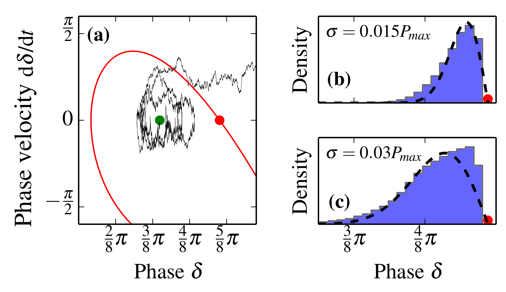
The saddle point itself is characterized by a vanishing velocity . Almost all trajectories leave the basin with a non-vanishing velocity ( i.e. ‘above’ the saddle point in the phase space portrait shown in Fig. 2). More precisely, the probability density of the trajectory on the basin boundary in phase space is given by a Weibull function [31]
| (6) |
where is a normalization constant. This theoretical prediction is equally well confirmed by the numerical simulations as shown in Fig. 2 on the right. With increasing noise amplitude the distribution gets broader, i.e. the escape velocity increases.
Escape via the weakest link.– To maintain a stable operation it is essential to know not only under which conditions, but also how power system operation may become unstable. We first consider a simple system of two identical generators coupled to a bulk power grid with transmission lines of different capacity, both being subject to independent and identically distributed Gaussian white noise (see Fig. 3 (a)). Either of the two generators can become unstable, such that the grid can escape the basin of attraction of the stable phase-locked state via two different routes. The mean escape time is still described by Kramer’s rate for intermediate damping, when we take into account that the lower potential barrier along both routes determines the escape (see Fig. 3 (b)). The two-dimensional potential is then given as
| (7) |
In the limit of weak noise the escape problem is fully determined by the path with the smallest potential barrier . To illustrate this we vary the capacity of the transmission line connecting generator to the bulk grid while the capacity of the other line remains fixed. For the robustness is dominated by generator , whose connection is weaker. The exponent in Kramer’s formula (5) then crucially depends on the value of . Indeed, the exponent obtained from the numerical simulations again matches the theoretical predictions well in terms of the potential barrier (see Fig. 3 (c)). If we increase beyond , the other transmission line becomes the Achilles’ heal of the grid. The potential barrier and hence the exponent in Kramer’s formula thus no longer depend on . Yet, the non-exponential pre-factor in the formula (5) increases by increasing further because the relative transmission line load of the overall system decreases. When the noise becomes stronger, the sharp transition between the two possible escape routes gradually blurs, such that the more strongly connected generator can become unstable too (see Fig. 3 (d)).
Robustness of complex power grids.– In power grids with a less simple structure, it is essential to understand how the topology determines the robustness and to identify possible ways of instability. This enables a precise improvement of the grid and the elimination of weak links. Figure 4 (a) shows the stable fixed point in a grid with four generator and eight consumer nodes. The consumer dynamics also follows Eq. (2), but with . A fluctuating input can lead to a loss of synchrony and eventually to a system-wide failure. But where does this instability emerge and which of the transmission lines is most vulnerable?
We simulate the dynamics with all machines subject to independent and identically distributed white noise and record which transmission line becomes overloaded first, i.e. we record for which link the phase difference first crosses . In this way we identify four transmission lines which are vulnerable. Strikingly, these vulnerable lines are not necessarily the ones which are most heavily loaded in the first place. The loss of synchrony in a complex grid is a collective process, which cannot fully be understood from fundamental properties of single nodes or lines [32, 33].
Instead, Kramer’s theory tells that the saddle points of the entire dynamical system are decisive: As above, the grid leaves the basin of attraction of the stable phase-locked state in the vicinity of the saddle points. In a complex network, many saddle points may exist. But for the application of Kramer’s theory we only need to consider those saddle points with the lowest potential barrier, as escape through all other saddle points is exponentially suppressed. For the system studied here, these saddle points are calculated systematically using a method introduced in [34]. This method classifies the saddle points by the number of links where the phase difference exceeds . Typically, the higher this number, the higher is the potential barrier.
For the sample network depicted in Fig.4 for illustration, this method yields four saddle points with a comparably low potential barrier, all contributing to the escape process (four lower panels). All four saddles have exactly one line where the phase difference exceeds . The static analysis thus yields four vulnerable lines which exactly match the lines where overloads have been recorded in the numerical simulations. Even more, Kramer’s rate with the respective barrier heights again predicts the exit probabilities (not shown).
Conclusion. – In this Letter we have analyzed how high-frequency fluctuations impact the dynamical robustness of electric power grids. Focusing on Gaussian white noise yielded analytical access, thereby providing deeper insights into the collective dynamics of fluctuation-driven networks. To characterize the robustness of this stochastic system, we derived the scaling of escape times as a function of the grid load, inertia, damping and the noise amplitude. Furthermore, we demonstrated how power networks may escape the regime of stable operation. The grid escapes in the vicinity of (saddle) fixed points with a low potential barrier. Interestingly, these can typically be assigned to a single overloaded link, thus revealing the weak links of the grid.
Complementary work on power grid fluctuations [24] addresses the impact of intermittent noise and incorporates features of real wind turbines. Such settings avert the analytic treatment in terms of Kramer’s escape theory. The analytic approach presented in this Letter reveals which factors limit the robustness of power grid operation to fluctuating inputs. The results may thus not only provide efficient methodology to analyze fluctuation-driven oscillatory systems but may also help planning grid extensions to assure dynamic stability and robustness in future highly renewable power systems.
We gratefully acknowledge support from the Federal Ministry of Education and Research (BMBF grant no. 03SF0472A-E), the Helmholtz Association (via the joint initiative “Energy System 2050 - A Contribution of the Research Field Energy” and the grant no. VH-NG-1025 to D.W.), the Göttingen Graduate School for Neurosciences and Molecular Biosciences (DFG Grant GSC 226/2) to B.S. and the Max Planck Society to M.T.
References
- [1] S. M. Amin and B. F. Wollenberg, IEEE Power and Energy Magazine 3, 34 (2005).
- [2] T. Bruckner et al., in Climate Change 2014: Mitigation of Climate Change. Contribution of Working Group III to the Fifth Assessment Report of the Intergovernmental Panel on Climate Change, edited by O. Edenhofer et al. (Cambridge University Press, Cambridge, United Kingdom, 2014).
- [3] S. H. Strogatz, Nature 410, 268 (2001).
- [4] E. Marris, Nature 454, 570 (2008).
- [5] C. D. Brummitt, P. D. H. Hines, I. Dobson, C. Moore, and R. M. D’Souza, Proceedings of the National Academy of Sciences 110, 12159 (2013).
- [6] M. Timme, L. Kocarev, and D. Witthaut, New J. Phys. 17, 110201 (2015).
- [7] R. Sims et al., in IPCC Special Report on Renewable Energy Sources and Climate Change Mitigation, edited by O. Edenhofer et al. (Cambridge University Press, Cambridge, United Kingdom, 2011).
- [8] D. Heide, L. Von Bremen, M. Greiner, C. Hoffmann, M. Speckmann, and S. Bofinger, Renewable Energy 35, 2483 (2010).
- [9] P. Milan, M. Wächter, and J. Peinke, Phys. Rev. Lett. 110, 138701 (2013).
- [10] M. Anvari, G. Lohmann, M. Wächter, P. Milan, E. Lorenz, D. Heinemann, M. R. R. Tabar, and J. Peinke, New J. Phys. 18, 063027 (2016).
- [11] A. Ulbig, T. S. Borsche, and G. Andersson, IFAC Proceedings Volumes 47, 7290 (2014).
- [12] J. Machowski, J. Bialek, and J. Bumby, Power system dynamics, stability and control (John Wiley & Sons, New York, 2008).
- [13] G. Filatrella, A. H. Nielsen, and N. F. Pedersen, Eur. Phys. J. B 61, 485 (2008).
- [14] M. Rohden, A. Sorge, M. Timme, and D. Witthaut, Phys. Rev. Lett. 109, 064101 (2012).
- [15] A. E. Motter, S. A. Myers, M. Anghel, and T. Nishikawa, Nature Physics 9, 191 (2013).
- [16] T. Nishikawa and A. E. Motter, New J. Phys. 17, 015012 (2015).
- [17] A. J. Wood, B. F. Wollenberg, and G. B. Sheblé, Power Generation, Operation and Control (John Wiley & Sons, New York, 2013).
- [18] M. Rohden, A. Sorge, D. Witthaut, and M. Timme, Chaos 24, 013123 (2014).
- [19] F. Dörfler, M. Chertkov, and F. Bullo, Proceedings of the National Academy of Sciences 110, 2005 (2013).
- [20] B. Schäfer, M. Matthiae, M. Timme, and D. Witthaut, New Journal of Physics 17, 015002 (2015).
- [21] T. Pesch, H.-J. Allelein, and J.-F. Hake, Eur. Phys. J. Special Topics 223, 2561 (2014).
- [22] See supplemental material at [url will be inserted by publisher] for discussion of robustness of the phenomena reported and a comparison of the escape time across different power grid models.
- [23] J. W. Simpson-Porco, F. Dörfler, and F. Bullo, IFAC Proceedings Volumes 45, 264 (2012).
- [24] K. Schmietendorf, O. Kamps, and J. Peinke, arXiv preprint arXiv:1611.08235 (2016).
- [25] H. A. Kramers, Physica 7, 284 (1940).
- [26] N. van Kampen, Stochastic processes in physics and chemistry (Elsevier, Amsterdam, 1992).
- [27] P. Hänggi, P. Talkner, and M. Borkovec, Reviews of modern physics 62, 251 (1990).
- [28] C. W. Gardiner, Handbook of stochastic methods for physics, chemistry, and the natural sciences (Springer Berlin, 2004).
- [29] H. Risken, The Fokker-Planck Equation (Springer, Berlin, 1984).
- [30] D. Manik, D. Witthaut, B. Schäfer, M. Matthiae, A. Sorge, M. Rohden, E. Katifori, and M. Timme, Eur. Phys. J. Special Topics 223, 2527 (2014).
- [31] Z. Schuss, Theory and applications of stochastic processes - an analytical approach (Springer, New York, 2010).
- [32] D. Witthaut, M. Rohden, X. Zhang, S. Hallerberg, and M. Timme, Phys. Rev. Lett. 116, 138701 (2016).
- [33] P. Crucitti, V. Latora, and M. Marchiori, Physica A: Statistical mechanics and its applications 338, 92 (2004).
- [34] D. Manik, M. Timme, and D. Witthaut, arXiv preprint arXiv:1611.09825 (2016).
- [35] M. Calabria, W. Schumacher, J. M. Guerrero, J. C. Vasquez, and X. Zhao, in 2015 IEEE 6th International Symposium on PEDG (IEEE, 2015), pp. 1–9.
- [36] J. W. Simpson-Porco, F. Dörfler, and F. Bullo, Automatica 49, 2603 (2013).
- [37] S. Auer, K. Kleis, P. Schultz, J. Kurths, and F. Hellmann, Eur. Phys. J. Special Topics 225, 609 (2016).
- [38] S. D’Arco and J. A. Suul, in PowerTech (POWERTECH), 2013 IEEE Grenoble (IEEE, 2013), pp. 1–7.
- [39] J. Schiffer, D. Goldin, J. Raisch, and T. Sezi, in Decision and Control (CDC), 2013 IEEE 52nd Annual Conference on (IEEE, 2013), pp. 2334–2339.
- [40] K. Schmietendorf, J. Peinke, R. Friedrich, and O. Kamps, Eur. Phys. J. Special Topics 223, 2577 (2014).
- [41] J. Ma, Y. Sun, X. Yuan, J. Kurths, and M. Zhan, PloS one 11, e0165943 (2016).
Supplemental Material
accompanying the manuscript
Escape Routes, Weak Links, and Desynchronization in Fluctuation-driven
Networks
Benjamin Schäfer
Moritz Matthiae
Xiaozhu Zhang
Martin Rohden
Marc Timme
Dirk Witthaut
Appendix A Overview
Power grids are complex systems and may be described on different levels of detail [12]. A cornerstone model of power system dynamics is the swing equation - a second order differential equation describing the mechanical rotation of synchronous machines. The mechanical phase angle typically equals the voltage phase angle, such that it also determines the power flows in the grid. This model is studied in the main text for heavily loaded lines. In this Supplemental Material we provide additional arguments why this model is appropriate and explore different parameter regimes, in particular less heavily loaded lines and the effects of a decreasing inertia.
Furthermore, we analyze the robustness of different power system models against noise. Wind turbines and photovoltaics are usually connected to a grid via power electronic inverters. Power electronic devices can act as virtual synchronous machines described by the swing equation, otherwise they should be described as first-order Kuramoto oscillators [35, 23, 36]. The swing equation is known to describe the short-term dynamical stability of a power system. On longer time scales the assumption of a constant voltage may no longer be satisfied [37]. In this Supplemental Material we study grids without inertia in terms of a first-order model and state the appropriate escape rate formula. In addition, we investigate the effects of voltage variability numerically in terms of the third-order model. For simplicity of presentation, we focus on the scenario of one machine connected to the bulk grid.
Appendix B Power Grid Models
First, we define an effective potential in terms of the voltage phase as
| (8) |
with effective power produced and capacity parameter of a line , which describes the maximal transmittable power of that line. In terms of this potential, the swing equation, i.e., the equations of motion for the voltage phase and its angular velocity becomes
| (9) |
with the reference angular velocity Hz, damping , inertia and Gaussian white noise with standard deviation . Parameters used (if not stated otherwise) are , , , . In a fully renewable power grid, which is dominated by wind and solar power production, there will be fewer rotating machines than today and the inertia will be smaller. In the extreme case all rotating machines are replaced by inverters feeding wind and solar power into the grid. However, it has been demonstrated that inverters can be used to act similar to synchronous machines by providing virtual inertia, see e.g. [38, 39]. Again, the dynamics of the inverters is preferentially modelled by using the swing equation (9).
Furthermore, we note that the swing equation (9) is also used in coarse grained models [12, 11]. In those models, multiple machines are aggregated into a coherent subgroup. Each node, representing one sub group, is then described as an oscillatory machine with effective power , damping and inertia . The dynamics is again described by the swing equation.
If we model a system without physical or virtual inertia, each node is best described as a Kuramoto oscillator [35, 36, 23] with the equation of motion being
| (10) |
In the main text we assumed the voltage amplitude to stay constant even in the scenario of a heavily loaded grid. Here, we consider the third order model [40, 12, 37, 41] which allows the voltage amplitude to vary over time:
| (11) |
with the voltage time scale , bulk voltage , , , and the voltage droop . For and the voltage remains at the fixed point at all times and reproduces the second order model while for deviations from the second order model can be observed. Typical parameter values are taken from [40].
Appendix C Calculation of
Appendix D Mean escape time
We simulate the system consisting of one generator coupled to the bulk and extract the scaling of the escape time , depending on the noise amplitude , the inertia and the voltage droop for the first, second and third order model. For the sake of consistency and comparability, we define the escape time as that instance when the system passed and did not return to the fixed point. Although this does not correspond exactly to the boundary of the basin of attraction, it enables us to compare these three different models.
D.1 2nd Order: Scaling with respect to inertia
Decreasing inertia in the swing equation (9), decreases the escape time and thereby the stability of the system, see fig. S.5. This dependency is well-described in Kramer’s escape theory
| (15) |
with
| (16) |
and
| (17) |
as stated in the main manuscript.
D.2 2nd Order: Less loaded lines
In the main text we only considered highly loaded lines with , i.e., the lines were close to maximum load. In fig. S.6 we display that Kramer’s escape theory also holds for less loaded scenarios. We observe a good agreement of the numerical results and the analytical prediction by eq. (15). The noise amplitude needs to be increased significantly compared to less loaded scenarios, see, e.g. fig. S.5, to arrive at similar escape times .
D.3 First order model
In contrast to the 2nd order model, the 1st order model has only one globally stable fixed point at and we observe transitions from to with . In a real system, the fast change of the angle would almost certainly destabilize the system as the power flow along the line given by would change dramatically during the course of this transition and would most likely violate security regulations [12]. We obtain Kramer’s escape rate for the first order model [26] as
| (18) |
and demonstrate perfect agreement of theory and simulations in fig. S.7.
D.4 Third order model
The fixed point for the angle in the third order system is given as [40]. For sufficiently small values of the voltage droop , the voltage amplitude tends to the stable fixed point . With increasing this fixed point gets destabilized and the mean escape time of the system decreases. This effect might change for larger values of . Our theory using Kramer’s escape rate correctly predicts the stability as long as the voltage changes are sufficiently slow or small, see fig. S.8.