跳到论文正文
W Papers独立论文阅读器 arXiv:1611.08043 论文正文 计算阅读时间 · 0%
引用这篇论文根据当前论文元数据生成,正式投稿前建议核对。


License: arXiv.org perpetual non-exclusive license
arXiv:1611.08043v1 [math-ph] 24 Nov 2016

Generalized Kubo Formulas for the Transport Properties of Incommensurate 2D Atomic Heterostructures

Eric Cancès Affiliation: CERMICS, Ecole des Ponts and Inria Paris Affiliation: 6 & 8 avenue Blaise Pascal Affiliation: 77455 Marne-la-Vallée Cedex 2, France Email: eric.cances@enpc.fr    Paul Cazeaux Affiliation: School of Mathematics Affiliation: University of Minnesota Affiliation: Minneapolis, Minnesota 55455 Email: pcazeaux@umn.edu    Mitchell Luskin Affiliation: School of Mathematics Affiliation: University of Minnesota Affiliation: Minneapolis, Minnesota 55455 Email: luskin@umn.edu
Abstract

We give an exact formulation for the transport coefficients of incommensurate two-dimensional atomic multilayer systems in the tight-binding approximation. This formulation is based upon the C∗C^{*} algebra framework introduced by Bellissard and collaborators [3, 2] to study aperiodic solids (disordered crystals, quasicrystals, and amorphous materials), notably in the presence of magnetic fields (quantum Hall effect). We also present numerical approximations and test our methods on a one-dimensional incommensurate bilayer system.

1 Introduction

The synthesis and modeling of layered two-dimensional atomic heterostructures is currently being intensely investigated with the goal of designing materials with desired electronic and optical properties [12]. These multilayer two-dimensional materials are generally incommensurate, that is, the multilayer system does not have a periodic structure although each individual layer does have a periodic structure.

Despite the scientific and technological importance of incommensurate materials, an exact formulation has not yet been given for important properties such as the electronic density of states or the electrical conductivity. The typical approach to modeling and computing the properties of incommensurate structures is to approximate them by commensurate structures or supercells [22]. Although this approach might provide a good approximation in many cases, the error is generally uncontrolled (see [8] for an analysis of the supercell approximation of the mechanical relaxation of coupled incommensurate chains). Further, the approximation of the important case of small angle rotated bilayer structures requires supercell sizes that are too large for numerical solution [23]. In this paper, we give such an exact formulation and develop numerical approximations.

Within independent electron or mean field models such as Hartree-Fock or Kohn-Sham, the electronic density of states and transport properties for periodic structures can be rigorously formulated by the use of the Bloch transform to obtain generalized eigenstates of the Hamiltonian as a plane wave with wave vector in the Brillouin zone (𝐤\mathbf{k}-space) multiplied by a periodic function. This approach leads to the classical Kubo formulae for the transport properties of periodic solids which can be formulated as the trace of corresponding operators [14].

Although incommensurate multilayer two-dimensional materials no longer have a periodic structure and the local environment of each atom is unique, this local environment can be simply characterized by shifts of each layer. Further, the shifts corresponding to the local environments are uniformly distributed over the periodic unit cell of each layer. One can then develop generalized Kubo formulae for incommensurate heterostructures by considering the integral over the uniformly distributed shifts of the trace of operators that depend of the corresponding local environment.

To give a precise formulation and enable mathematical and numerical analysis, we apply the C∗C^{*}-algebra approach for aperiodic solids introduced by Bellissard and collaborators [3, 2] to incommensurate heterostructures. Following these lines, we can characterize the incommensurate structure by its hull, which is a compact description of the local environments. We first present the construction of the hull for perfect multilayers in Sections 2.1 and 2.2. The case of disordered heterostructures is dealt with in Section 2.3.

In Section 3, we present the C∗C^{*}-algebra formalism for tight-binding models. Rather than working with operators on the infinite dimensional tight-binding state space, the C∗C^{*}-algebra approach allows us to exploit the simplification of working directly with a C∗C^{*}-algebra of functions which represent the operators of interest. Within the tight-binding model that we consider, we obtain a compact parametrization of the tight-binding Hamiltonian by using environment-dependent site and hopping functions [11]. The C∗C^{*}-algebra approach then allows us to concisely construct transport operators and their trace by utilizing the algebra structure. After introducing the abstract setting in Section 3.1, we describe the special case of perfect incommensurate bilayers in full detail in Section 3.2.

In Section 4, we present a new, minimalistic one-dimensional toy model to showcase the expected effects of incommensurability in coupled multilayered systems. We chose to introduce here a simple discretization based on periodic supercells and on the Kernel Polynomial Method [25]. In future works, we will develop more sophisticated approaches based on the C∗C^{*}-algebras introduced in this paper. We will present their numerical analysis, using the C∗C^{*}-algebra formalism, and use the minimalistic model introduced in this paper as a benchmark to analyze and test different implementation strategies, possibly targeting directly incommensurate cases, for computing the density of states, the conductivity or other observables. One such possible strategy is to exploit locality [17, 6].

Previous research on the development of numerical methods to approximate transport properties within the C∗C^{*}-algebra formulation has been done by Prodan [18] for the effects of disorder and magnetic fields. Recent work on the analysis and computation of the density of states for incommensurate layers from the operator point of view is given in [17]. We note that the density of states is defined in [17] as a thermodynamic limit, while the density of states and transport properties are given explicit expressions in the C∗C^{*}-algebra approach, which directly provide the values of the quantities of interest in the thermodynamic limit.

2 Geometries of multi-layered systems

2.1 Perfect multilayer structure

Refer to caption
Figure 1: Example of a heterostructure: stack of five monolayers

Heterostructures are vertical stacks of a few two-dimensional crystalline monolayers. An example is depicted in Figure 1. Five distinct layers with different atomic components and structures are positioned as a vertical stack. Due to the weak van der Waals nature of the interactions between these layers, they do not relax into a common periodic structure, but rather each layer essentially keeps the structure it possesses as an isolated monolayer. The resulting assembly is thus in general not periodic: it is an aperiodic structure with a long-range order. A systematic model of heterostructures starts naturally by a rigorous depiction of this particular geometry, which can be idealized in the following way.

For the sake of generality, we consider dd-dimensional systems embedded in (d+1)(d+1)-dimensional space. Note that we choose dd as the natural dimension of the structure, since the (d+1)(d+1)st dimension plays a very particular and limited role, especially in tight-binding models. We are in particular interested in d=2d=2 for the layered heterostructures which motivate our study, while the choice d=1d=1 enables us to present simple numerical examples in Section 4.

Let us consider such a (d+1)(d+1)-dimensional system of pp parallel dd-dimensional periodic atomic layers denoted ℒj⊂ℝd+1\mathcal{L}_{j}\subset\mathbb{R}^{d+1}, j=1​…​pj=1\dots p. We denote by

  • –

    (𝐞1,⋯,𝐞d+1)(\mathbf{e}_{1},\cdots,\mathbf{e}_{d+1}) an orthonormal basis of the physical space such that each layer is perpendicular to 𝐞d+1\mathbf{e}_{d+1}; from now on we identify the physical space with ℝd+1\mathbb{R}^{d+1} using the cartesian coordinates 𝐱=(x1,⋯,xd+1)T\mathbf{x}=(x_{1},\cdots,x_{d+1})^{T} associated with this basis;

  • –

    hjh_{j} the (d+1)(d+1)st coordinate of the center of layer jj. Without loss of generality, we can assume that 0=h1<h2<⋯<hp0=h_{1}<h_{2}<\cdots<h_{p};

  • –

    ℛj\mathcal{R}_{j} the dd-dimensional periodic lattice of layer jj;

  • –

    𝐄j\mathbf{E}_{j} the matrix in ℝd×d\mathbb{R}^{d\times d} whose columns form a basis generating the lattice ℛj\mathcal{R}_{j}:

    ℛj:=𝐄j​ℤd⊂ℝd;\mathcal{R}_{j}:=\mathbf{E}_{j}\mathbb{Z}^{d}\subset\mathbb{R}^{d}; (1)
  • –

    Γj:=ℝd/ℛj\Gamma_{j}:=\mathbb{R}^{d}/\mathcal{R}_{j} the quotient of ℝd\mathbb{R}^{d} by the discrete lattice ℛj\mathcal{R}_{j}, which has the topology of a dd-dimensional torus and can be canonically identified with the periodic unit cell Γ^j:=𝐄j[−1/2,1/2)d\widehat{\Gamma}_{j}:=\mathbf{E}_{j}[-1/2,1/2)^{d} of layer jj;

  • –

    mjm_{j} the motif of layer jj, i.e., the measure on ℝd+1\mathbb{R}^{d+1} supported in Γ^j×ℝ\widehat{\Gamma}_{j}\times\mathbb{R} and representing the nuclear distribution ρjnuc\rho^{\rm nuc}_{j} of layer jj. More precisely, mjm_{j} is a finite sum of positively weighted Dirac measures of the form

    mj=∑k=1Mjzk(j)​δ𝐱k(j),m_{j}=\sum_{k=1}^{M_{j}}z_{k}^{(j)}\delta_{\mathbf{x}_{k}^{(j)}},

    where MjM_{j} is the number of nuclei per unit cell in layer jj, z1(j),⋯,zMj(j)z_{1}^{(j)},\cdots,z_{M_{j}}^{(j)} the atomic charges of these nuclei, and 𝐱k(j)∈Γ^j×ℝ\mathbf{x}_{k}^{(j)}\in\widehat{\Gamma}_{j}\times\mathbb{R} their positions in a reference configuration in which the center of layer jj belongs to the plane xd+1=0x_{d+1}=0. The nuclear distribution ρjnuc\rho^{\rm nuc}_{j} of layer jj is then given by

    ρjnuc=∑𝐧j∈ℛjmj(⋅−(𝜸j+𝐧j+hj𝐞d+1))=∑𝐧j∈ℛj∑k=1Mjzk(j)δ𝜸j+𝐧j+𝐱k(j)+hj​𝐞d+1,\rho^{\rm nuc}_{j}=\sum_{\mathbf{n}_{j}\in\mathcal{R}_{j}}m_{j}\left(\cdot-(\boldsymbol{\gamma}_{j}+\mathbf{n}_{j}+h_{j}\mathbf{e}_{d+1})\right)=\sum_{\mathbf{n}_{j}\in\mathcal{R}_{j}}\sum_{k=1}^{M_{j}}z_{k}^{(j)}\delta_{\boldsymbol{\gamma}_{j}+\mathbf{n}_{j}+\mathbf{x}_{k}^{(j)}+h_{j}\mathbf{e}_{d+1}},

    where 𝜸j∈Γ^j\boldsymbol{\gamma}_{j}\in\widehat{\Gamma}_{j} depends on the horizontal position of the lattice sites of layer jj relatively to the origin of the coordinates. Here and in the sequel, we use the same notation to denote a vector 𝐲\mathbf{y} of ℝd\mathbb{R}^{d} and its canonical embedding (𝐲T,0)T(\mathbf{y}^{T},0)^{T} in ℝd+1\mathbb{R}^{d+1}.

Remark 2.1.

Note that, by virtue of the identification Γj≡Γ^j\Gamma_{j}\equiv\widehat{\Gamma}_{j}, an equivalence class 𝛄j∈Γj\boldsymbol{\gamma}_{j}\in\Gamma_{j} can be seen either as a discrete set of points in ℝd\mathbb{R}^{d}, or as one point of the periodic unit cell Γ^j\widehat{\Gamma}_{j}. Since both viewpoints are employed here, we denote these two usages differently to avoid confusion:

  • –

    𝜸j\boldsymbol{\gamma}_{j} will be used to denote a single point of the periodic unit cell Γ^j\widehat{\Gamma}_{j},

  • –

    𝜸j+ℛj\boldsymbol{\gamma}_{j}+\mathcal{R}_{j} will be used to denote the corresponding set of points in ℝd\mathbb{R}^{d}. In particular, the sum of the values of a function ff over the lattice sites of layer jj will be denoted as ∑𝐩j∈𝜸j+ℛjf⁡(𝐩j)\sum_{\mathbf{p}_{j}\in\boldsymbol{\gamma}_{j}+\mathcal{R}_{j}}f(\mathbf{p}_{j}).

2.2 Translation group and the hull

To understand the geometry of our heterostructures, it is a useful exercise to picture the origin of coordinates as our viewpoint (in the sense of ”position of observation”). Neighboring atoms then constitute a local environment, e.g., A-A stacking (aligned layers) vs. A-B stacking (staggered layers) in a graphene bilayer [10]. This environment, i.e., the positions of all atoms relative to the origin, constitutes a choice of configuration for the structure.

In the case of a periodic material (a perfect crystal), the set of such possible configurations, or the hull [2], is simply the periodic unit cell. Indeed, choosing the origin at points which differ only by a lattice vector results in identical configurations. This invariance by lattice translations is what enables the classical use of the Bloch theorem to reduce the Hamiltonian operator set on the whole space to a family of easily analyzed operators on the periodic unit cell, indexed by the quasimomenta 𝐤\mathbf{k} belonging to the Brillouin zone of the crystal.

This is not the case for the generically incommensurate layered structures presented in Section 2.1. The change of coordinate origin (our viewpoint) is naturally associated with the action of the group ℝd\mathbb{R}^{d} on ℝd+1\mathbb{R}^{d+1} by translations 𝚃\mathtt{T} that are parallel to the layers:

For 𝐚∈ℝd,𝚃𝐚:{ℝd+1→ℝd+1,𝐱↦(x1+a1,…,xd+ad,xd+1).\text{For }\mathbf{a}\in\mathbb{R}^{d},\qquad{\mathtt{T}}_{\mathbf{a}}:\left\{\begin{aligned} \mathbb{R}^{d+1}&\to\mathbb{R}^{d+1},\\ \mathbf{x}&\mapsto\left(x_{1}+a_{1},\dots,x_{d}+a_{d},x_{d+1}\right).\end{aligned}\right. (2)
Remark 2.2.

Note that there is no translational symmetry in the perpendicular (d+1)(d+1)st-dimension, and therefore we need not include this direction in the continuous translation group. The situation is different in discrete (tight-binding) models, where we model hopping from layer to layer as will be seen later on.

Now we proceed with the formal definition of the hull. The positions of all the atoms are encoded in the nuclear charge distribution, a Radon measure in 𝔐⁡(ℝd+1)\mathfrak{M}(\mathbb{R}^{d+1}) [2], on which the translation group ℝd\mathbb{R}^{d} acts naturally11 1 Given 𝐚∈ℝd\mathbf{a}\in\mathbb{R}^{d}, the translation 𝚃𝐚\mathtt{T}_{\mathbf{a}} acts on the space of continuous functions with compact support 𝒞c​(ℝd+1)\mathcal{C}_{c}(\mathbb{R}^{d+1}) through 𝚃𝐚​f​(𝐱)=f⁡(𝚃−𝐚​𝐱)\mathtt{T}_{\mathbf{a}}f(\mathbf{x})=f(\mathtt{T}_{-\mathbf{a}}\mathbf{x}). Therefore it acts on the space 𝔐⁡(ℝd+1)\mathfrak{M}(\mathbb{R}^{d+1}) of Radon measures through 𝚃𝐚​μ​(f)=μ⁡(𝚃−𝐚​f)\mathtt{T}_{\mathbf{a}}\mu(f)=\mu\left(\mathtt{T}_{-\mathbf{a}}f\right) whenever f∈𝒞c​(ℝd+1)f\in\mathcal{C}_{c}(\mathbb{R}^{d+1}) and μ∈𝔐⁡(ℝd+1)\mu\in\mathfrak{M}(\mathbb{R}^{d+1}).. Then the hull is the dynamical system (Ω,ℝd,𝚃)(\Omega,\mathbb{R}^{d},\mathtt{T}), where Ω\Omega is the closure of the orbit of the nuclear charge distribution measure on ℝd+1\mathbb{R}^{d+1} generated by the atoms of all pp layers under the action of ℝd\mathbb{R}^{d} through 𝚃\mathtt{T}.

Refer to caption
(a) Top view of the crystalline structure
Refer to caption
(b) Projection of the origin into the unit cells
Figure 2: Illustration of the process for labeling the local configurations of heterostructures. The vertices of the parallelograms are sites of the shifted lattices γj+ℛj\gamma_{j}+\mathcal{R}_{j}.

Parameterizing this orbit is similar to describing the position of all atoms relative to the origin, given an arbitrary translation of the system. An example of this process is presented by Figure 2 (see also Figure 3 for a simple one-dimensional picture). While the initial view of all atomic positions in Figure 2(a) might appear quite chaotic, it can actually be efficiently encoded. Since each individual layer ℒj\mathcal{L}_{j}, j=1,…,pj=1,\dots,p is periodic, the set of all possible configurations for layer jj is in one-to-one correspondence with Γj\Gamma_{j}. Indeed, an element 𝜸j∈Γj\boldsymbol{\gamma}_{j}\in\Gamma_{j} is the projection of the jj-th layer periodic lattice on the horizontal plane, i.e., an equivalence class modulo ℛj\mathcal{R}_{j}, as seen in Figure 2(b). The overall configuration can thus be parameterized as an element of

Ω=Γ1×⋯×Γp.\Omega=\Gamma_{1}\times\cdots\times\Gamma_{p}. (3)
Figure 3: Schematic representation of a configuration ω=(𝜸1,𝜸2,𝜸3,𝜸4)∈Ω\omega=(\boldsymbol{\gamma}_{1},\boldsymbol{\gamma}_{2},\boldsymbol{\gamma}_{3},\boldsymbol{\gamma}_{4})\in\Omega for d=1d=1 and p=4p=4. The vector 𝜸j\boldsymbol{\gamma}_{j} on the figure corresponds to the unique representative of the equivalence class 𝜸j\boldsymbol{\gamma}_{j} in the periodic unit cell Γ^j\widehat{\Gamma}_{j} and 𝜸1+ℛ1\boldsymbol{\gamma}_{1}+\mathcal{R}_{1} is the set of the lattice points of the first layer in the configuration ω\omega.

The hull Ω\Omega therefore has the topology of a (d​p)(dp)-dimensional torus. For any given configuration ω=(𝜸1,…,𝜸p)\omega=(\boldsymbol{\gamma}_{1},\dots,\boldsymbol{\gamma}_{p}), the nuclear charge distribution is

ρωnuc=∑j=1p(∑𝐩j∈𝜸j+ℛj𝚃𝐩jmj(⋅−hj𝐞d+1)).\rho^{\rm nuc}_{\omega}=\sum_{j=1}^{p}\left(\sum_{\mathbf{p}_{j}\in\boldsymbol{\gamma}_{j}+\mathcal{R}_{j}}\mathtt{T}_{\mathbf{p}_{j}}m_{j}(\cdot-h_{j}\mathbf{e}_{d+1})\right).

The support of the measure ρωnuc\rho^{\rm nuc}_{\omega} is the discrete set:

{ℒω:=⋃j=1pℒjω⊂ℝd+1 (set of all atomic positions), with ​ℒjω:=Supp​(mj)+𝜸j+ℛj+hj​𝐞d+1 (atomic positions in layer j).\left\{\begin{aligned} &\mathcal{L}^{\omega}:=\bigcup_{j=1}^{p}\mathcal{L}_{j}^{\omega}\subset\mathbb{R}^{d+1}&\text{ (set of all atomic positions)},\\ &\text{ with }\mathcal{L}_{j}^{\omega}:=\textrm{Supp}(m_{j})+\boldsymbol{\gamma}_{j}+\mathcal{R}_{j}+h_{j}\mathbf{e}_{d+1}&\text{ (atomic positions in layer $j$)}.\end{aligned}\right. (4)

There exists a natural action of the additive ℝd\mathbb{R}^{d} group on Ω\Omega, corresponding to an horizontal translation of the whole system in the previous parameterization, defined by

𝚃𝐚​(𝜸1,…,𝜸p)=(𝜸1+𝐚,…,𝜸p+𝐚).\mathtt{T}_{\mathbf{a}}(\boldsymbol{\gamma}_{1},\dots,\boldsymbol{\gamma}_{p})=\left(\boldsymbol{\gamma}_{1}+\mathbf{a},\dots,\boldsymbol{\gamma}_{p}+\mathbf{a}\right). (5)

For convenience, we use the same notation 𝚃{\mathtt{T}} to denote the action of the translation group ℝd\mathbb{R}^{d} on ℝd+1\mathbb{R}^{d+1}, formula (2), and on Ω\Omega, formula (5).

Finally, the dynamical system (Ω,ℝd,𝚃)(\Omega,\mathbb{R}^{d},\mathtt{T}) is equipped with a probability measure ℙ\mathbb{P} which encodes the relative occurrences of the various configurations. This measure should be invariant by the translation action to reflect the spatial homogeneity of the system. There is here a unique such measure under the incommensurability condition given in the following definition. Let us denote the dual (or reciprocal) lattice of any cocompact22 2 Recall that a cocompact lattice ℛ\mathcal{R} of ℝd\mathbb{R}^{d} is a discrete periodic lattice of ℝd\mathbb{R}^{d} with dd free vectors (in such a way that ℝd/ℛ\mathbb{R}^{d}/\mathcal{R} is compact), and that the dual lattice of a cocompact lattice ℛ\mathcal{R} is defined by ℛ∗={𝐤∈ℝd|𝐤⋅𝐧∈ℤ,∀𝐧∈ℛ}.\mathcal{R}^{*}=\left\{\mathbf{k}\in\mathbb{R}^{d}\ |\ \mathbf{k}\cdot\mathbf{n}\in\mathbb{Z},\quad\forall\mathbf{n}\in\mathcal{R}\right\}. When ℛ\mathcal{R} is generated by the columns of a matrix 𝐄\mathbf{E}, its dual ℛ∗\mathcal{R}^{*} is generated by the columns of (𝐄T)−1(\mathbf{E}^{T})^{-1}, the inverse transpose of 𝐄\mathbf{E}. lattice ℛ\mathcal{R} by ℛ∗\mathcal{R}^{*}.

Definition 2.3.

The collection of cocompact lattices ℛ1,⋯,ℛp\mathcal{R}_{1},\cdots,\mathcal{R}_{p} of ℝd\mathbb{R}^{d} is called incommensurate if we have for any pp-tuple (𝐤1,…,𝐤p)∈ℛ1∗×⋯×ℛp∗(\mathbf{k}_{1},\dots,\mathbf{k}_{p})\in\mathcal{R}_{1}^{*}\times\cdots\times\mathcal{R}_{p}^{*},

∑j=1p𝐤j=𝟎⇔𝐤j=𝟎∀j=1,…,p.\sum_{j=1}^{p}\mathbf{k}_{j}=\mathbf{0}\quad\Leftrightarrow\quad\mathbf{k}_{j}=\mathbf{0}\ \ \forall j=1,\dots,p. (6)

This definition, surprising at first, defines incommensurability as the absence of constructive interferences, or Bragg reflections, between the lattices. The following result proves that it is also the right condition for the layered system to have a homogeneous character, i.e., all possible configurations will be visited uniformly as we translate our viewpoint along the horizontal place.

Proposition 2.4.

Let ℛ1,⋯,ℛp\mathcal{R}_{1},\cdots,\mathcal{R}_{p} of ℝd\mathbb{R}^{d} be cocompact lattices of ℝd\mathbb{R}^{d}, Γj=ℝd/ℛj\Gamma_{j}=\mathbb{R}^{d}/\mathcal{R}_{j}, and Ω=Γ1×⋯×Γp\Omega=\Gamma_{1}\times\cdots\times\Gamma_{p}, endowed with the uniform probability measure ℙ\mathbb{P}. Then,

  1. 1.

    ℙ\mathbb{P} is invariant by the translation group ℝd\mathbb{R}^{d};

  2. 2.

    the dynamical system (Ω,ℝd,𝚃,ℙ)(\Omega,\mathbb{R}^{d},\mathtt{T},\mathbb{P}) is uniquely ergodic if and only if the lattices ℛ1,⋯,ℛp\mathcal{R}_{1},\cdots,\mathcal{R}_{p} are incommensurate. In this case, we have the Birkhoff property: for any f∈C⁡(Ω)f\in C(\Omega) and ω∈Ω\omega\in\Omega,

    limr→∞1|Br|​∫Brf⁡(𝚃−𝐚​ω)​𝑑𝐚=∫Ωf​𝑑ℙ,\lim_{r\to\infty}\frac{1}{|B_{r}|}\int_{B_{r}}f(\mathtt{T}_{-\mathbf{a}}\omega)\mathrm{d}\mathbf{a}=\int_{\Omega}f\mathrm{d}\mathbb{P}, (7)

    where BrB_{r} is the ball of radius rr centered at zero.

Proof.

The first point follows from the definition (5) and the translation invariance of the Lebesgue measure. To show that incommensurability implies ergodicity, we will make use of the following lemma:

Lemma 2.5.

Let ℛ\mathcal{R} be a lattice in ℝd\mathbb{R}^{d} and 𝐤∈ℝd\mathbf{k}\in\mathbb{R}^{d}. Then:

limr→∞1#⁡(ℛ∩Br)∑𝐧∈ℛ∩Bre2​i​π​𝐤⋅𝐧=0⇔𝐤∉ℛ∗.\lim_{r\to\infty}\frac{1}{\#\left(\mathcal{R}\cap B_{r}\right)}\sum_{\mathbf{n}\in\mathcal{R}\cap B_{r}}e^{2i\pi\mathbf{k}\cdot\mathbf{n}}=0\quad\Leftrightarrow\quad\mathbf{k}\notin\mathcal{R}^{*}. (8)

It is clear that if 𝐤∈ℛ∗\mathbf{k}\in\mathcal{R}^{*}, then the weighted sum in the left-hand side in (8) is always equal to 11 for all r>0r>0, and thus the limit is not zero. Let (𝐜1,…,𝐜d)(\mathbf{c}_{1},\dots,\mathbf{c}_{d}) be a basis of ℛ\mathcal{R} and (𝐜1∗,…,𝐜d∗)(\mathbf{c}^{*}_{1},\dots,\mathbf{c}^{*}_{d}) the associated dual basis of ℛ∗\mathcal{R}^{*} (𝐜j⋅𝐜k∗=δj​k\mathbf{c}_{j}\cdot\mathbf{c}_{k}^{*}=\delta_{jk}). We assume now that 𝐤∉ℛ∗\mathbf{k}\notin\mathcal{R}^{*}, and expanding 𝐤=k1​𝐜1∗+⋯+kd​𝐜d∗\mathbf{k}=k_{1}\mathbf{c}_{1}^{*}+\dots+k_{d}\mathbf{c}_{d}^{*}, we suppose that k1∉ℤk_{1}\notin\mathbb{Z} without loss of generality.

Let ℰr⟂\mathcal{E}_{r}^{\perp} be the projection of ℛ∩Br\mathcal{R}\cap B_{r} onto the last (d−1)(d-1) lattice coordinates:

ℰr⟂={(n2,…,nd)∈ℤd−1|∃n1∈ℤ,∑j=1dnj𝐜j∈ℛ∩Br}.\mathcal{E}_{r}^{\perp}=\left\{(n_{2},\dots,n_{d})\in\mathbb{Z}^{d-1}\quad\biggr|\quad\exists n_{1}\in\mathbb{Z},\ \sum_{j=1}^{d}n_{j}\mathbf{c}_{j}\in\mathcal{R}\cap B_{r}\right\}.

There exists for any (d−1)(d-1)-tuple 𝐧~=(n2,…,nd)\widetilde{\mathbf{n}}=(n_{2},\dots,n_{d}) in ℰr⟂\mathcal{E}_{r}^{\perp} two integers Nr±​(𝐧~)N_{r}^{\pm}(\widetilde{\mathbf{n}}) such that for any n1∈ℤn_{1}\in\mathbb{Z}, ∑j=1dnj​𝐜j\sum_{j=1}^{d}n_{j}\mathbf{c}_{j} belongs to ℛ∩Br\mathcal{R}\cap B_{r} if and only if Nr−​(𝐧~)≤n1<Nr+​(𝐧~)N_{r}^{-}(\widetilde{\mathbf{n}})\leq n_{1}<N_{r}^{+}(\widetilde{\mathbf{n}}). We decompose accordingly the sum in (8):

∑𝐧∈ℛ∩Bre2​i​π​𝐤⋅𝐧\displaystyle\sum_{\mathbf{n}\in\mathcal{R}\cap B_{r}}e^{2i\pi\mathbf{k}\cdot\mathbf{n}} =∑𝐧~∈ℰr⟂∑n1=Nr−​(𝐧~)Nr+​(𝐧~)−1e2​i​π​(k1​n1+𝐤~⋅𝐧~)\displaystyle=\sum_{\widetilde{\mathbf{n}}\in\mathcal{E}_{r}^{\perp}}\sum_{n_{1}=N_{r}^{-}(\widetilde{\mathbf{n}})}^{N_{r}^{+}(\widetilde{\mathbf{n}})-1}e^{2i\pi\left(k_{1}n_{1}+\widetilde{\mathbf{k}}\cdot\widetilde{\mathbf{n}}\right)}
=∑𝐧~∈ℰr⟂e2​i​π​𝐤~⋅𝐧~​(e2​i​π​k1​Nr−​(𝐧~)−e2​i​π​k1​Nr+​(𝐧~)1−e2​i​π​k1).\displaystyle=\sum_{\widetilde{\mathbf{n}}\in\mathcal{E}_{r}^{\perp}}e^{2i\pi\widetilde{\mathbf{k}}\cdot\widetilde{\mathbf{n}}}\left(\frac{e^{2i\pi k_{1}N_{r}^{-}(\widetilde{\mathbf{n}})}-e^{2i\pi k_{1}N_{r}^{+}(\widetilde{\mathbf{n}})}}{1-e^{2i\pi k_{1}}}\right).

We can bound the number of elements in (ℛ∩Br)\left(\mathcal{R}\cap B_{r}\right) from below by c1​rdc_{1}r^{d} and of ℰr⟂\mathcal{E}_{r}^{\perp} by c2​rd−1c_{2}r^{d-1} where c1,c2>0c_{1},c_{2}>0 are two geometrical constants depending only on ℛ\mathcal{R}. Thus

|1#⁡(ℛ∩Br)​∑𝐧∈ℛ∩Bre2​i​π​𝐤⋅𝐧|≤(2|1−e2​i​π​k1|)​c2c1​r.\left|\frac{1}{\#\left(\mathcal{R}\cap B_{r}\right)}\sum_{\mathbf{n}\in\mathcal{R}\cap B_{r}}e^{2i\pi\mathbf{k}\cdot\mathbf{n}}\right|\leq\left(\frac{2}{|1-e^{2i\pi k_{1}}|}\right)\frac{c_{2}}{c_{1}r}.

Since k1∉ℤk_{1}\notin\mathbb{Z}, Lemma 2.5 is proved.

Birkhoff property. Let us now suppose that the collection of lattices ℛ1,⋯,ℛp\mathcal{R}_{1},\cdots,\mathcal{R}_{p} is incommensurate. Let f∈C⁡(Ω)f\in C(\Omega) and ω=(𝜸1,…,𝜸p)∈Ω\omega=(\boldsymbol{\gamma}_{1},\dots,\boldsymbol{\gamma}_{p})\in\Omega. Let ε>0\varepsilon>0 and TεT_{\varepsilon} be a trigonometric polynomial such that ‖f−Tε‖∞≤ε\|f-T_{\varepsilon}\|_{\infty}\leq\varepsilon. TεT_{\varepsilon} is a finite linear combination of Fourier factors of the form

G𝐤1,…,𝐤p:(𝜸1,…,𝜸p)↦e2​i​π​(𝐤1⋅𝜸1+⋯+𝐤p⋅𝜸p) with (𝐤1,…,𝐤p)∈ℛ1∗×⋯×ℛp∗.G_{\mathbf{k}_{1},\dots,\mathbf{k}_{p}}:(\boldsymbol{\gamma}_{1},\dots,\boldsymbol{\gamma}_{p})\mapsto e^{2i\pi(\mathbf{k}_{1}\cdot\boldsymbol{\gamma}_{1}+\cdots+\mathbf{k}_{p}\cdot\boldsymbol{\gamma}_{p})}\quad\text{ with }\quad(\mathbf{k}_{1},\dots,\mathbf{k}_{p})\in\mathcal{R}_{1}^{*}\times\cdots\times\mathcal{R}_{p}^{*}.

If 𝐤j=𝟎\mathbf{k}_{j}=\boldsymbol{0} for all j=1,…,pj=1,\dots,p, then clearly

limr→∞1|Br|​∫BrG𝟎,…,𝟎​(𝚃−𝐚​ω)​𝑑𝐚=1=∫ΩG𝟎,…,𝟎​𝑑ℙ.\lim_{r\to\infty}\frac{1}{|B_{r}|}\int_{B_{r}}G_{\boldsymbol{0},\dots,\boldsymbol{0}}(\mathtt{T}_{-\mathbf{a}}\omega)\mathrm{d}\mathbf{a}=1=\int_{\Omega}G_{\boldsymbol{0},\dots,\boldsymbol{0}}\mathrm{d}\mathbb{P}.

Otherwise, we assume without loss of generality that 𝐤2≠𝟎\mathbf{k}_{2}\neq\boldsymbol{0}, and we approximate the ball BrB_{r} for r>0r>0 by a union of translated unit cells,

Br1=⋃𝐧1∈ℛ1∩Br(Γ^1+𝐧1)where Γ^1=𝐄1[−1/2,1/2)d.B^{1}_{r}=\bigcup_{\mathbf{n}_{1}\in\mathcal{R}_{1}\cap B_{r}}\left(\widehat{\Gamma}_{1}+\mathbf{n}_{1}\right)\qquad\text{where }\widehat{\Gamma}_{1}=\mathbf{E}_{1}[-1/2,1/2)^{d}.

Averaging over this approximate ball, we find:

1|Br1|\displaystyle\frac{1}{|B_{r}^{1}|} ∫Br1G𝐤1,…,𝐤p​(𝚃−𝐚​ω)​𝑑𝐚=|Γ^1|−1#⁡(ℛ1∩Br)​∑𝐧1∈ℛ1∩Br∫Γ^1e2​i​π​∑j=1p𝐤j⋅(𝜸j−𝐚−𝐧1)​𝑑𝐚\displaystyle\int_{B^{1}_{r}}G_{\mathbf{k}_{1},\dots,\mathbf{k}_{p}}(\mathtt{T}_{-\mathbf{a}}\omega)\mathrm{d}\mathbf{a}=\frac{|\widehat{\Gamma}_{1}|^{-1}}{\#\left(\mathcal{R}_{1}\cap B_{r}\right)}\sum_{\mathbf{n}_{1}\in\mathcal{R}_{1}\cap B_{r}}\int_{\widehat{\Gamma}_{1}}e^{2i\pi\sum_{j=1}^{p}\mathbf{k}_{j}\cdot(\boldsymbol{\gamma}_{j}-\mathbf{a}-\mathbf{n}_{1})}\mathrm{d}\mathbf{a}
=(|Γ^1|−1∫Γ^1e2​i​π​∑j=1p𝐤j⋅(𝜸j−𝐚)d𝐚)1#⁡(ℛ1∩Br)∑𝐧1∈ℛ1∩Bre−2iπ∑j=2p𝐤j⋅𝐧1.\displaystyle=\left(|\widehat{\Gamma}_{1}|^{-1}\int_{\widehat{\Gamma}_{1}}e^{2i\pi\sum_{j=1}^{p}\mathbf{k}_{j}\cdot(\boldsymbol{\gamma}_{j}-\mathbf{a})}\mathrm{d}\mathbf{a}\right)\frac{1}{\#\left(\mathcal{R}_{1}\cap B_{r}\right)}\sum_{\mathbf{n}_{1}\in\mathcal{R}_{1}\cap B_{r}}e^{-2i\pi\sum_{j=2}^{p}\mathbf{k}_{j}\cdot\mathbf{n}_{1}}.

We assume that the lattices ℛ1,⋯,ℛp\mathcal{R}_{1},\cdots,\mathcal{R}_{p} are incommensurate, and thus ∑j=2p𝐤j∈ℛ1∗\sum_{j=2}^{p}\mathbf{k}_{j}\in\mathcal{R}_{1}^{*} if and only if 𝐤j=𝟎\mathbf{k}_{j}=\boldsymbol{0} for all j=2,…,pj=2,\dots,p. This is not possible since 𝐤2≠𝟎\mathbf{k}_{2}\neq\boldsymbol{0}, and we therefore deduce from Lemma 2.5 that, uniformly in ω\omega,

limr→∞1|Br1|​∫Br1G𝐤1,…,𝐤p​(𝚃−𝐚​ω)​𝑑𝐚=0.\lim_{r\to\infty}\frac{1}{|B_{r}^{1}|}\int_{B^{1}_{r}}G_{\mathbf{k}_{1},\dots,\mathbf{k}_{p}}(\mathtt{T}_{-\mathbf{a}}\omega)\mathrm{d}\mathbf{a}=0.

Note that for some C>0C>0 independent of rr, we have |Br​Δ​Br1|≤C​rd−1|B_{r}\Delta B^{1}_{r}|\leq Cr^{d-1} (where A​Δ​BA\Delta B denotes the symmetric difference of the sets AA and BB). Thus we conclude

∀(𝐤1,…,𝐤p)∈(ℛ1∗×⋯×ℛp∗)∖{𝟎},limr→∞1|Br|∫BrG𝐤1,…,𝐤p(𝚃−𝐚ω)d𝐚=0, uniformly in ω.\forall(\mathbf{k}_{1},\dots,\mathbf{k}_{p})\in(\mathcal{R}_{1}^{*}\times\cdots\times\mathcal{R}_{p}^{*})\setminus\left\{{\mathbf{0}}\right\},\quad\lim_{r\to\infty}\frac{1}{|B_{r}|}\int_{B_{r}}G_{\mathbf{k}_{1},\dots,\mathbf{k}_{p}}(\mathtt{T}_{-\mathbf{a}}\omega)\mathrm{d}\mathbf{a}=0,\text{ uniformly in }\omega.

As a result, the trigonometric polynomial TεT_{\varepsilon} satisfies for r>0r>0 large enough, uniformly in ω\omega,

|1|Br|​∫BrTε​(𝚃−𝐚​ω)​𝑑𝐚−∫ΩTε​𝑑ℙ|≤ε.\left|\frac{1}{|B_{r}|}\int_{B_{r}}T_{\varepsilon}(\mathtt{T}_{-\mathbf{a}}\omega)\mathrm{d}\mathbf{a}-\int_{\Omega}T_{\varepsilon}\mathrm{d}\mathbb{P}\right|\leq\varepsilon.

Finally, since ‖f−Tε‖∞≤ε\|f-T_{\varepsilon}\|_{\infty}\leq\varepsilon we obtain the Birkhoff ergodic formula: for rr large enough, uniformly in ω\omega,

|1|Br|​∫Brf⁡(𝚃−𝐚​ω)​𝑑𝐚−∫Ωf​𝑑ℙ|≤3​ε.\left|\frac{1}{|B_{r}|}\int_{B_{r}}f(\mathtt{T}_{-\mathbf{a}}\omega)\mathrm{d}\mathbf{a}-\int_{\Omega}f\mathrm{d}\mathbb{P}\right|\leq 3\varepsilon. (9)

Ergodicity. Let BB be a measurable subset of Ω\Omega invariant under the action of ℝd\mathbb{R}^{d}. Let ε>0\varepsilon>0 and fεf_{\varepsilon} be a continuous function such that ‖χB−fε‖L1​(Ω)≤ε\|\chi_{B}-f_{\varepsilon}\|_{L^{1}(\Omega)}\leq\varepsilon. By invariance of BB under translations, we have for all 𝐚∈ℝd\mathbf{a}\in\mathbb{R}^{d},

‖fε∘𝚃𝐚−fε‖L1​(Ω)≤2​ε.\|f_{\varepsilon}\circ\mathtt{T}_{\mathbf{a}}-f_{\varepsilon}\|_{L^{1}(\Omega)}\leq 2\varepsilon.

We can bound the difference between fεf_{\varepsilon} and its Birkhoff means:

‖1|Br|​∫Brfε∘𝚃−𝐚​𝑑𝐚−fε‖L1​(Ω)\displaystyle\left\|\frac{1}{|B_{r}|}\int_{B_{r}}f_{\varepsilon}\circ\mathtt{T}_{-\mathbf{a}}\mathrm{d}\mathbf{a}-f_{\varepsilon}\right\|_{L^{1}(\Omega)} =∫Ω|1|Br|​∫Brfε​(𝚃−𝐚​ω)​𝑑𝐚−fε​(ω)|​𝑑ℙ​(ω)\displaystyle=\int_{\Omega}\left|\frac{1}{|B_{r}|}\int_{B_{r}}f_{\varepsilon}(\mathtt{T}_{-\mathbf{a}}\omega)\mathrm{d}\mathbf{a}-f_{\varepsilon}(\omega)\right|\mathrm{d}\mathbb{P}(\omega)
≤1|Br|​∫Br∫Ω|fε​(𝚃−𝐚​ω)−fε​(ω)|​𝑑ℙ​(ω)​𝑑𝐚≤2​ε,\displaystyle\leq\frac{1}{|B_{r}|}\int_{B_{r}}\int_{\Omega}\left|f_{\varepsilon}(\mathtt{T}_{-\mathbf{a}}\omega)-f_{\varepsilon}(\omega)\right|\mathrm{d}\mathbb{P}(\omega)\mathrm{d}\mathbf{a}\leq 2\varepsilon,

where we have used the triangle inequality for integrals and Fubini’s theorem for non-negative functions. Since the Birkhoff means of fεf_{\varepsilon} converge uniformly in ω\omega for r→∞r\to\infty to ∫Ωfε​𝑑ℙ\int_{\Omega}f_{\varepsilon}\mathrm{d}\mathbb{P}, we deduce that

‖∫Ωfε​𝑑ℙ−fε‖L1​(Ω)≤2​ε.\left\|\int_{\Omega}f_{\varepsilon}\mathrm{d}\mathbb{P}-f_{\varepsilon}\right\|_{L^{1}(\Omega)}\leq 2\varepsilon.

As a consequence, we have by the triangle inequality,

‖χB−ℙ⁡(B)‖L1​(Ω)≤‖χB−fε‖L1​(Ω)+‖fε−∫Ωfε​𝑑ℙ‖L1​(Ω)+‖∫Ωfε​𝑑ℙ−ℙ⁡(B)‖L1​(Ω)≤4​ε.\displaystyle\|\chi_{B}-\mathbb{P}(B)\|_{L^{1}(\Omega)}\leq\|\chi_{B}-f_{\varepsilon}\|_{L^{1}(\Omega)}+\left\|f_{\varepsilon}-\int_{\Omega}f_{\varepsilon}\mathrm{d}\mathbb{P}\right\|_{L^{1}(\Omega)}+\left\|\int_{\Omega}f_{\varepsilon}\mathrm{d}\mathbb{P}-\mathbb{P}(B)\right\|_{L^{1}(\Omega)}\leq 4\varepsilon.

Since this holds for any ε>0\varepsilon>0, we conclude that χB\chi_{B} is constant a.s., and therefore ℙ⁡(B)∈{0,1}\mathbb{P}(B)\in\{0,1\}. Thus ℙ\mathbb{P} is ergodic.

Non-averaging case. If the lattices ℛ1,…,ℛp\mathcal{R}_{1},\dots,\mathcal{R}_{p} are not incommensurate, there exists a particular nonzero combination (𝐤1,…,𝐤p)∈ℛ1∗×⋯×ℛp∗(\mathbf{k}_{1},\dots,\mathbf{k}_{p})\in\mathcal{R}_{1}^{*}\times\cdots\times\mathcal{R}_{p}^{*} such that ∑j=1p𝐤j=𝟎\sum_{j=1}^{p}\mathbf{k}_{j}=\boldsymbol{0}. Then, we have for the corresponding Fourier factor,

G𝐤1,…,𝐤p​(𝚃−𝐚​ω)=G𝐤1,…,𝐤p​(ω),∀(𝐚,ω)∈ℝd×Ω.\displaystyle G_{\mathbf{k}_{1},\dots,\mathbf{k}_{p}}(\mathtt{T}_{-\mathbf{a}}\omega)=G_{\mathbf{k}_{1},\dots,\mathbf{k}_{p}}(\omega),\qquad\forall(\mathbf{a},\omega)\in\mathbb{R}^{d}\times\Omega.

The function G𝐤1,…,𝐤pG_{\mathbf{k}_{1},\dots,\mathbf{k}_{p}} is then invariant by the ℝd\mathbb{R}^{d}-action and not constant. Therefore the dynamical system (Ω,ℝd,𝚃,ℙ)(\Omega,\mathbb{R}^{d},\mathtt{T},\mathbb{P}) is not ergodic in this case. ∎

Remark 2.6.

When the lattices ℛ1,⋯,ℛp\mathcal{R}_{1},\cdots,\mathcal{R}_{p} are commensurate, i.e., ⋂j=1pℛj\bigcap_{j=1}^{p}\mathcal{R}_{j} forms a cocompact superlattice of ℝd\mathbb{R}^{d}, then the orbits through the action 𝚃\mathtt{T} of ℝd\mathbb{R}^{d} on Ω\Omega are no longer dense in Ω\Omega, rather they form lower dimensional submanifolds of Ω\Omega which are then distinct hulls for the possible configurations. In this case, Bloch theory allows one to study each of these nonequivalent configuration sets individually.

Remark 2.7.

Note that the lattices ℛ1,⋯,ℛp\mathcal{R}_{1},\cdots,\mathcal{R}_{p} can also be neither commensurate nor incommensurate. We do not know if one can always find a sensible parameterization of the hull of a particular configuration in this case, since its orbit under ℝd\mathbb{R}^{d} may not be dense in Ω\Omega, nor has a simple geometry.

2.3 Disordered multilayer systems

The case of disordered multilayer systems is more involved. For the sake of both brevity and clarity, we consider the specific, but representative, example of a bilayer system whose bottom layer lays on a periodic substrate modeled by an external ℛ0\mathcal{R}_{0}-periodic potential, and whose top layer may have defects. We denote by ℛ0\mathcal{R}_{0} the periodic lattice of the substrate, and by ℛ1\mathcal{R}_{1} and ℛ2\mathcal{R}_{2} the periodic lattices of the bottom and top layers respectively, and we assume that ℛ0\mathcal{R}_{0}, ℛ1\mathcal{R}_{1} and ℛ2\mathcal{R}_{2} are incommensurate in the sense of Definition 2.3. We then assume that the defects are such that

  • –

    the overall geometry of the system is not modified: the periodic lattice ℛ2\mathcal{R}_{2} is still appropriate to describe the configurations of the system; the difference with the case of ”perfect” homogeneous systems dealt with in the previous section, is that the nuclear distribution inside the unit cells of the top layer is not the same in each cell;

  • –

    in each cell in the top layer, the motif can be one of the following: (m2(0),m2(1),⋯,m2(D))(m_{2}^{(0)},m_{2}^{(1)},\cdots,m_{2}^{(D)}), where m2(0)m_{2}^{(0)} is the periodic motif of the top layer in the absence of defects, and m2(1),⋯,m2(D)m_{2}^{(1)},\cdots,m_{2}^{(D)} correspond to the different kinds of defects that can be observed. For instance, in the case of a graphene layer for which each carbon atom can adsorb a hydrogen atom, there are two carbon atoms in each cell, m2(0)m_{2}^{(0)} corresponds to the case when no hydrogen atom is adsorbed, m2(1)m_{2}^{(1)} (respectively, m2(2)m_{2}^{(2)}) to the case when only the first (respectively, second) carbon atom has adsorbed a hydrogen atom, and m2(3)m_{2}^{(3)} to the case when the two carbon atoms have adsorbed hydrogen atoms;

  • –

    the defects are independently and identically distributed in the cells of the top layer. We denote by (p0,p1,⋯,pD)(p_{0},p_{1},\cdots,p_{D}) (with pj>0p_{j}>0 and ∑j=0Dpj=1\sum_{j=0}^{D}p_{j}=1) the probability distribution of the motifs (m2(0),m2(1),⋯,m2(D))(m_{2}^{(0)},m_{2}^{(1)},\cdots,m_{2}^{(D)}).

Without loss of generality, we can assume that the center of the bottom layer is contained in the plane xd+1=0x_{d+1}=0, and that the center of the top layer is contained in the plane xd+1=h>0x_{d+1}=h>0. For each point in 𝐫∈ℝd\mathbf{r}\in\mathbb{R}^{d}, we introduce the decomposition of 𝐫\mathbf{r} associated with the lattice ℛ2\mathcal{R}_{2} defined as

𝐫=[𝐫]2+{𝐫}2 with [𝐫]2∈ℛ2 and {𝐫}2∈Γ^2=𝐄2[−1/2,1/2)d.\mathbf{r}=\left[\mathbf{r}\right]_{2}+\left\{\mathbf{r}\right\}_{2}\qquad\text{ with }\left[\mathbf{r}\right]_{2}\in\mathcal{R}_{2}\text{ and }\left\{\mathbf{r}\right\}_{2}\in\widehat{\Gamma}_{2}=\mathbf{E}_{2}[-1/2,1/2)^{d}. (10)

For this example, the hull is the dynamical system (Ω,ℝd,τ,ℙ)(\Omega,\mathbb{R}^{d},\tau,\mathbb{P}) where

  • –

    Ω=Γ0×Γ1×Γ2×{0,1,⋯,D}ℛ2\Omega=\Gamma_{0}\times\Gamma_{1}\times\Gamma_{2}\times\left\{0,1,\cdots,D\right\}^{\mathcal{R}_{2}}, the configuration ω=(𝜸0,𝜸1,𝜸2,{t𝐧2}𝐧2∈ℛ2)∈Ω\omega=(\boldsymbol{\gamma}_{0},\boldsymbol{\gamma}_{1},\boldsymbol{\gamma}_{2},\left\{t_{\mathbf{n}_{2}}\right\}_{\mathbf{n}_{2}\in\mathcal{R}_{2}})\in\Omega corresponding to the nuclear distribution

    ρωnuc=∑𝐩1∈𝜸1+ℛ1T𝐩1m1+∑𝐩2∈𝜸2+ℛ2T𝐩2m2(t[𝐩2]2)(⋅−h𝐞d+1).\rho^{\rm nuc}_{\omega}=\sum_{\mathbf{p}_{1}\in\boldsymbol{\gamma}_{1}+\mathcal{R}_{1}}T_{\mathbf{p}_{1}}m_{1}+\sum_{\mathbf{p}_{2}\in\boldsymbol{\gamma}_{2}+\mathcal{R}_{2}}T_{\mathbf{p}_{2}}m_{2}^{(t_{[\mathbf{p}_{2}]_{2}})}(\cdot-h\mathbf{e}_{d+1}).

    Here t[𝐩2]2∈{0,1,⋯,D}t_{[\mathbf{p}_{2}]_{2}}\in\left\{0,1,\cdots,D\right\} is the type of the motif carried by the cell of the top layer centered at 𝐩2+h​𝐞d+1\mathbf{p}_{2}+h\mathbf{e}_{d+1}. Note that γ0\gamma_{0} does not appear in the definition of ρωnuc\rho^{\rm nuc}_{\omega}, since we do not take into account the geometry relaxation of the bilayer system due to the interaction with the substrate. On the other hand, the substrate generates a ℛ0\mathcal{R}_{0}-periodic potential which modifies the electronic structure of the bilayer system, and this potential depends on γ0\gamma_{0}, the relative position of the substrate with respect to the bilayer system;

  • –

    τ\tau is the action of the group ℝd\mathbb{R}^{d} on Ω\Omega defined by

    ∀𝐚∈ℝd,∀\displaystyle\forall\mathbf{a}\in\mathbb{R}^{d},\quad\forall ω=(𝜸0,𝜸1,𝜸2,{t𝐧2}𝐧2∈ℛ2),\displaystyle\omega=(\boldsymbol{\gamma}_{0},\boldsymbol{\gamma}_{1},\boldsymbol{\gamma}_{2},\left\{t_{\mathbf{n}_{2}}\right\}_{\mathbf{n}_{2}\in\mathcal{R}_{2}}),
    τ𝐚​(ω)=(𝜸0+𝐚,𝜸1+𝐚,𝜸2+𝐚,{t𝐧2−[{𝜸2}2+𝐚]2}𝐧2∈ℛ2);\displaystyle\tau_{\mathbf{a}}(\omega)=(\boldsymbol{\gamma}_{0}+\mathbf{a},\boldsymbol{\gamma}_{1}+\mathbf{a},\boldsymbol{\gamma}_{2}+\mathbf{a},\left\{t_{\mathbf{n}_{2}-[\{\boldsymbol{\gamma}_{2}\}_{2}+\mathbf{a}]_{2}}\right\}_{\mathbf{n}_{2}\in\mathcal{R}_{2}});
  • –

    denoting by μ\mu the probability on the set {0,1,⋯,D}\left\{0,1,\cdots,D\right\} with law (p0,p1,⋯,pD)(p_{0},p_{1},\cdots,p_{D}), the ergodic probability ℙ\mathbb{P} on Ω\Omega is defined as

    ℙ=ℙ0⊗ℙ1⊗ℙ2⊗ℙdis,\mathbb{P}=\mathbb{P}_{0}\otimes\mathbb{P}_{1}\otimes\mathbb{P}_{2}\otimes\mathbb{P}_{\rm dis},

    where ℙj\mathbb{P}_{j} is the uniform probability distribution on Γj\Gamma_{j}, and ℙdis=μ⊗ℛ2\mathbb{P}_{\rm dis}=\mu^{\otimes\mathcal{R}_{2}} is the probability distribution on the disorder.

3 C∗-algebra formalism for tight-binding models

In this section, we adapt to the tight-binding modeling of perfect multilayer atomic heterostructures the C∗C^{*}-algebra formalism which was extensively used by Belissard and collaborators [3, 2] to model and analyze transport in aperiodic solids.

In the framework of tight-binding models, it is appropriate (see Remark 2.2) to use the following alternative definition of the hull:

  • –

    ΩD={1,⋯,p}×Ω\displaystyle\Omega_{\rm D}=\left\{1,\cdots,p\right\}\times\Omega;

  • –

    𝔱\mathfrak{t} is the action of the group

    𝔾D=ℤ/p​ℤ×ℝd\mathbb{G}_{\rm D}=\mathbb{Z}/p\mathbb{Z}\times\mathbb{R}^{d}

    defined by: for all a=(α,𝐚)∈𝔾Da=(\alpha,\mathbf{a})\in\mathbb{G}_{\rm D}, and all (j,𝜸1,⋯,𝜸p)∈ΩD(j,\boldsymbol{\gamma}_{1},\cdots,\boldsymbol{\gamma}_{p})\in\Omega_{\rm D},

    𝔱a​(j,𝜸1,⋯,𝜸p)=(j−α,𝜸1+𝐚,⋯,𝜸p+𝐚),\mathfrak{t}_{a}(j,\boldsymbol{\gamma}_{1},\cdots,\boldsymbol{\gamma}_{p})=(j-\alpha,\boldsymbol{\gamma}_{1}+\mathbf{a},\cdots,\boldsymbol{\gamma}_{p}+\mathbf{a}),

    where the −- sign in j−αj-\alpha refers to the natural action of ℤ/p​ℤ\mathbb{Z}/p\mathbb{Z} on {1,⋯,p}\left\{1,\cdots,p\right\} (if α=k+p​ℤ\alpha=k+p\mathbb{Z}, j−α=((j−k−1)modp)+1j-\alpha=((j-k-1)\mod p)+1);

  • –

    ℙD\mathbb{P}_{\rm D} is as usual the uniform probability distribution on ΩD\Omega_{\rm D}, and it is ergodic if and only if the lattices ℛ1,…,ℛp\mathcal{R}_{1},\dots,\mathcal{R}_{p} are incommensurate.

More explicitly, for non-disordered multilayers, ΩD\Omega_{\rm D} consists of pp copies of Γ1×⋯×Γp\Gamma_{1}\times\cdots\times\Gamma_{p} indexed by j∈{1,⋯,p}j\in\left\{1,\cdots,p\right\} such that the reference lattice site of the configuration is in layer jj.

In the tight-binding representation, the quantum states are expanded on a finite number of orbitals in each periodic unit cell, for example a set of maximally localized Wannier orbitals [24, 15, 16]. We therefore introduce, for each layer kk, a finite set Ξk\Xi_{k} of tight-binding orbitals per unit cell. For a given configuration ω=(j,𝜸1,⋯,𝜸p)\omega=(j,\boldsymbol{\gamma}_{1},\cdots,\boldsymbol{\gamma}_{p}), the tight-binding orbital of type n∈Ξkn\in\Xi_{k} associated with the lattice site of layer kk located at point 𝐱+hk​𝐞d+1∈𝜸k+ℛk+hk​𝐞d+1\mathbf{x}+h_{k}\mathbf{e}_{d+1}\in\boldsymbol{\gamma}_{k}+\mathcal{R}_{k}+h_{k}\mathbf{e}_{d+1} is indexed by the triplet ((k−j)modp,𝐱,n)∈ℤ/p​ℤ×(γk+ℛk)×Ξk((k-j)\mod p,\mathbf{x},n)\in\mathbb{Z}/p\mathbb{Z}\times(\gamma_{k}+\mathcal{R}_{k})\times\Xi_{k}. The integer ((k−j)modp)((k-j)\mod p), considered as a element of ℤ/p​ℤ\mathbb{Z}/p\mathbb{Z}, accounts for the vertical jump (in terms of number of layers and modulo pp) to go from layer jj, which contains the origin in the configuration ω\omega, to layer kk (see also the graphical explanation in the one-dimensional case in Figure 4). This way of labeling the orbitals turns out to be well suited to the C∗C^{*}-algebra formalism introduced in the following two subsections.

The infinite set Ξω\Xi^{\omega} of all tight-biding orbitals of the pp layers is then indexed by:

Ξω=⋃k=1p{(k−j)modp}×(𝜸k+ℛk)×Ξk.\Xi^{\omega}=\bigcup_{k=1}^{p}\{(k-j)\mod p\}\times(\boldsymbol{\gamma}_{k}+\mathcal{R}_{k})\times\Xi_{k}. (11)

In the special case when there is only one orbital per unit cell, each Ξk\Xi_{k} only contains one element, and can therefore be omitted in the above definition of Ξω\Xi^{\omega}.

In the configuration ω\omega, the space of quantum states for the tight-binding model is

ℌω=ℓ2​(Ξω),\mathfrak{H}_{\omega}=\ell^{2}(\Xi^{\omega}), (12)

and observables such as the Hamiltonian are described as linear operators on ℌω\mathfrak{H}_{\omega}.

3.1 Abstract setting

Let us first briefly recall in this section the general formalism of groupoid C∗C^{*}-algebras. We refer e.g. to [3] for a more in-depth presentation of these mathematical objects. We further simplify the presentation by assuming that there is only one tight-binding orbital per unit cell in each layer, so that

Ξω≡⋃k=1p{(k−j)modp}×(𝜸k+ℛk)⊂𝔾D.\Xi^{\omega}\equiv\bigcup_{k=1}^{p}\{(k-j)\mod p\}\times(\boldsymbol{\gamma}_{k}+\mathcal{R}_{k})\subset\mathbb{G}_{D}. (13)

Note that this is not a restriction of the formalism (see Remark 3.1 below).

The first step is to construct a groupoid based on the canonical transversal XX of the hull ΩD\Omega_{D}:

X={ω∈ΩD|ω=(j,𝜸1,…,𝜸p);𝜸j=𝟎}.X=\left\{\omega\in\Omega_{D}\ |\ \omega=(j,\boldsymbol{\gamma}_{1},\dots,\boldsymbol{\gamma}_{p});\;\boldsymbol{\gamma}_{j}=\boldsymbol{0}\right\}. (14)

The idea is that while ΩD\Omega_{D} indexes the possible viewpoints from any point in the layer planes, each element of XX represents a possible unique viewpoint from the position of a lattice site, which is then chosen as the origin. This is a more appropriate approach in the case of tight-binding models. Associated with the transversal XX is the groupoid Γ⁡(X)\Gamma(X) defined as follows:

Γ⁡(X)={(ω,a)∈X×𝔾D|𝔱−a​ω∈X}.\Gamma(X)=\left\{(\omega,a)\in X\times\mathbb{G}_{D}\;|\;\mathfrak{t}_{-a}\omega\in X\right\}. (15)

For ω=(j,𝜸1,⋯,𝜸p)∈ΩD\omega=(j,\boldsymbol{\gamma}_{1},\cdots,\boldsymbol{\gamma}_{p})\in\Omega_{D} and a=(α,𝐚)∈GDa=(\alpha,\mathbf{a})\in G_{D}, (ω,a)∈Γ⁡(X)(\omega,a)\in\Gamma(X) if and only if 𝜸j=0\boldsymbol{\gamma}_{j}=0 and 𝜸j+α=𝐚\boldsymbol{\gamma}_{j+\alpha}=\mathbf{a}. Geometrically, Γ⁡(X)\Gamma(X) indexes all the possible jumps between two lattice sites in all possible configurations of the multilayer system. The physical space vector of the jump associated with (ω,a)(\omega,a) is 𝐀=𝐚+(hj+α−hj)​𝐞d+1\mathbf{A}=\mathbf{a}+(h_{j+\alpha}-h_{j})\mathbf{e}_{d+1}. The groupoid is equipped with a set of three operations, respectively the range r:Γ⁡(X)→Xr:\ \Gamma(X)\to X, source s:Γ⁡(X)→X,s:\Gamma(X)\to X, and composition ∘:Γ⁡(X)×Γ⁡(X)→Γ⁡(X)\circ:\Gamma(X)\times\Gamma(X)\to\Gamma(X), satisfying:

r⁡(ω,a)=ω,s⁡(ω,a)=𝔱−a​ω,(ω,a)∘(𝔱−a​ω,b)=(ω,a+b).r(\omega,a)=\omega,\qquad s(\omega,a)=\mathfrak{t}_{-a}\omega,\qquad(\omega,a)\circ(\mathfrak{t}_{-a}\omega,b)=(\omega,a+b). (16)

The fiber Γ(ω)\Gamma^{(\omega)} is defined as r−1​({ω})r^{-1}(\{\omega\}) for any ω∈X\omega\in X.

In a second step, we define the ∗-algebra 𝒜0\mathcal{A}_{0} of continuous functions with compact support defined on Γ⁡(X)\Gamma(X) with values in ℂ\mathbb{C}, endowed with the following composition laws and ∗-operator:

(λ​f)​(ω,a)\displaystyle(\lambda f)(\omega,a) =λ​f​(ω,a),\displaystyle=\lambda f(\omega,a), (17)
(f+g)​(ω,a)\displaystyle(f+g)(\omega,a) =f⁡(ω,a)+g⁡(ω,a),\displaystyle=f(\omega,a)+g(\omega,a),
(f∗g)​(ω,a)\displaystyle(f*g)(\omega,a) =∑(ω,b)∈Γ(ω)f⁡(ω,b)​g​(𝔱−b​ω,a−b),\displaystyle=\sum_{(\omega,b)\in\Gamma^{(\omega)}}f(\omega,b)g(\mathfrak{t}_{-b}\omega,a-b),
f∗​(ω,a)\displaystyle f^{*}(\omega,a) =f⁡(𝔱−a​ω,−a)¯.\displaystyle=\overline{f\left(\mathfrak{t}_{-a}\omega,-a\right)}.

The ∗-algebra 𝒜0\mathcal{A}_{0} has an identity, denoted by 𝟏\mathbf{1}:

𝟏​(ω,a)=δa,0.\mathbf{1}(\omega,a)=\delta_{a,0}.
Remark 3.1.

In the case when there are several atoms per unit cell, and/or each atom carries more than one orbital, the functions ff in (17) do not take their values in ℂ\mathbb{C} but f⁡(ω,a)f(\omega,a) is in ℂNj×Nj+α\mathbb{C}^{N_{j}\times N_{j+\alpha}} when ω=(j,𝛄1,…,𝛄p)\omega=(j,\boldsymbol{\gamma}_{1},\dots,\boldsymbol{\gamma}_{p}) and a=(α,𝐚)a=(\alpha,\mathbf{a}), where Nk=#⁡(Ξk)N_{k}=\#(\Xi_{k}) is the total number of tight-binding orbitals carried by the atoms in the unit cell of layer kk. Products of the form f⁡(ω,b)​g​(𝔱−b​ω,a−b)f(\omega,b)g(\mathfrak{t}_{-b}\omega,a-b) should then be understood as matrix products.

The ∗-algebra 𝒜0\mathcal{A}_{0} can be mapped onto a ∗-algebra of bounded linear operators acting on the space of quantum states ℌω=ℓ2​(Ξω)\mathfrak{H}_{\omega}=\ell^{2}(\Xi^{\omega}), see (12), via the representation formula:

πω​(f)​ϕ​(x)=∑(ω,y)∈Γ(ω)f⁡(𝔱−x​ω,y−x)​ϕ​(y),∀ϕ∈ℌω,∀x∈Ξω.\pi_{\omega}(f)\phi(x)=\sum_{(\omega,y)\in\Gamma^{(\omega)}}f\left(\mathfrak{t}_{-x}\omega,y-x\right)\phi(y),\qquad\forall\phi\in\mathfrak{H}_{\omega},\quad\forall x\in\Xi^{\omega}. (18)

In the above formula, we have implicitly used the fact that the set Ξω\Xi^{\omega} defined by (13) coincides with {y∈𝔾D|(ω,y)∈Γ(ω)}\left\{y\in\mathbb{G}_{D}\;|\;(\omega,y)\in\Gamma^{(\omega)}\right\}.

Figure 4: Graphical explanation of the representation formula (18) for d=1d=1, p=4p=4, and for a configuration ω=(3,𝜸1,𝜸2,𝟎,𝜸4)∈ΩD\omega=(3,\boldsymbol{\gamma}_{1},\boldsymbol{\gamma}_{2},{\mathbf{0}},\boldsymbol{\gamma}_{4})\in\Omega_{D}. The points x=(2−3,𝐱)=(−1,𝐱)x=(2-3,\mathbf{x})=(-1,\mathbf{x}) and y=(4−3,𝐲)=(1,𝐲)y=(4-3,\mathbf{y})=(1,\mathbf{y}) of Ξω\Xi^{\omega} are combined to form an element y−x=(2,𝐲−𝐱)y-x=(2,\mathbf{y}-\mathbf{x}) such that (𝔱−x​ω,y−x)∈Γ(𝔱−x​ω)(\mathfrak{t}_{-x}\omega,y-x)\in\Gamma^{({\mathfrak{t}_{-x}}\omega)}.

The following covariance condition holds: for a given γ=(ω,a)∈Γ⁡(X)\gamma=(\omega,a)\in\Gamma(X),

π𝔱−a​ω​(f)=𝔗​(γ)−1​πω​(f)​𝔗​(γ),\pi_{\mathfrak{t}_{-a}\omega}(f)=\mathfrak{T}(\gamma)^{-1}\pi_{\omega}(f)\mathfrak{T}(\gamma), (19)

where the translations 𝔗⁡(γ):ℌ𝔱−𝐚​ω→ℌω\mathfrak{T}(\gamma):\mathfrak{H}_{\mathfrak{t}_{-\mathbf{a}}\omega}\to\mathfrak{H}_{\omega} are unitary operators defined by

𝔗⁡(γ)​ϕ​(x)=ϕ⁡(𝔱−a​x),∀ϕ∈ℌ𝔱−a​ω,∀x∈Ξω.\mathfrak{T}(\gamma)\phi(x)=\phi(\mathfrak{t}_{-a}x),\qquad\forall\phi\in\mathfrak{H}_{\mathfrak{t}_{-a}\omega},\quad\forall x\in\Xi^{\omega}. (20)
Remark 3.2.

When d=2d=2, magnetic fields can be included in the description through a Peierls substitution term as follows. We assume that there is only one orbital per unit cell, and that the orbitals are carried by atoms located at the lattice sites. Let ℬ\mathscr{B} be an antisymmetric 3×33\times 3 matrix representing the magnetic field. For x=(l,𝐱)x=(l,\mathbf{x}) and y=(m,𝐲)y=(m,\mathbf{y}) in Ξω\Xi^{\omega} with ω=(j,𝛄1,…,𝛄p)\omega=(j,\boldsymbol{\gamma}_{1},\dots,\boldsymbol{\gamma}_{p}), we define the corresponding Peierls phase term as

Φℬω​(x,y)=π​∑ν,μ=13ℬν,μ​Xν​Yμ,\Phi^{\omega}_{\mathscr{B}}(x,y)=\pi\sum_{\nu,\mu=1}^{3}\mathrm{\mathscr{B}}_{\nu,\mu}X_{\nu}Y_{\mu}, (21)

where 𝐗=𝐱+(hj+l−hj)​𝐞3\mathbf{X}=\mathbf{x}+(h_{j+l}-h_{j})\mathbf{e}_{3} and 𝐘=𝐲+(hj+m−hj)​𝐞3\mathbf{Y}=\mathbf{y}+(h_{j+m}-h_{j})\mathbf{e}_{3} are the physical space vectors of the jumps from the origin to the sites xx and yy.

The product and representation formulae are then modified as

(f∗ℬg)​(ω,a)\displaystyle(f*_{\mathscr{B}}g)(\omega,a) =∑(ω,b)∈Γ(ω)f⁡(ω,b)​g​(𝔱−b​ω,a−b)​ei​Φℬω​(a,b),\displaystyle=\sum_{(\omega,b)\in\Gamma^{(\omega)}}f(\omega,b)g(\mathfrak{t}_{-b}\omega,a-b)e^{i\Phi^{\omega}_{\mathscr{B}}(a,b)}, (22)
πω​(f)​ϕ​(x)\displaystyle\pi_{\omega}(f)\phi(x) =∑(ω,y)∈Γ(ω)f(𝔱−xω,y−x)e−i​Φℬω​(x,y)ϕ(y),∀ϕ∈ℌω,x∈Ξω,\displaystyle=\sum_{(\omega,y)\in\Gamma^{(\omega)}}f\left(\mathfrak{t}_{-x}\omega,y-x\right)e^{-i\Phi^{\omega}_{\mathscr{B}}(x,y)}\phi(y),\qquad\forall\phi\in\mathfrak{H}_{\omega},x\in\Xi^{\omega},

where we again used the fact that Ξω={y∈𝔾D|(ω,y)∈Γ(ω)}\Xi^{\omega}=\left\{y\in\mathbb{G}_{D}\;|\;(\omega,y)\in\Gamma^{(\omega)}\right\}. In this case, the following covariance condition holds: for a given γ=(ω,a)∈Γ⁡(X)\gamma=(\omega,a)\in\Gamma(X),

π𝔱−a​ω​(f)=U​(γ)−1​πω​(f)​U​(γ),\pi_{\mathfrak{t}_{-a}\omega}(f)=U(\gamma)^{-1}\pi_{\omega}(f)U(\gamma), (23)

where the magnetic translations U⁡(γ):ℌ𝔱−a​ω→ℌωU(\gamma):\mathfrak{H}_{\mathfrak{t}_{-a}\omega}\to\mathfrak{H}_{\omega} are unitary operators defined by

U⁡(γ)​ϕ​(x)=exp⁡(i​∫[𝐗−𝐀,𝐗]𝒜⁡(y)⋅𝑑y)​ϕ​(𝔱−a​x),∀ϕ∈ℌ𝔱−a​ω,∀x∈Ξω.U(\gamma)\phi(x)=\mathrm{exp}\left(i\int_{[\mathbf{X}-\mathbf{A},\mathbf{X}]}\mathscr{A}(y)\cdot dy\right)\phi(\mathfrak{t}_{-a}x),\qquad\forall\phi\in\mathfrak{H}_{\mathfrak{t}_{-a}\omega},\quad\forall x\in\Xi^{\omega}. (24)

Here, 𝒜\mathscr{A} is a vector potential giving rise to the magnetic field ℬ\mathscr{B}, and [𝐗−𝐀,𝐗][\mathbf{X}-\mathbf{A},\mathbf{X}] is the line segment joining 𝐗−𝐀\mathbf{X}-\mathbf{A} to 𝐗\mathbf{X} in ℝ3\mathbb{R}^{3}.

Note that πω​(f)\pi_{\omega}(f) is hermitian if f=f∗f=f^{*}. This representation induces a C∗C^{*} norm on 𝒜0\mathcal{A}_{0}, defined by:

‖f‖=supω∈X‖πω​(f)‖,\|f\|=\sup_{\omega\in X}\|\pi_{\omega}(f)\|,

where the norm on the right hand side is the operator norm on ℒ⁡(ℌω)\mathcal{L}(\mathfrak{H}_{\omega}), the space of bounded linear operators on ℌω\mathfrak{H}_{\omega}. We then construct in a third and final step the C∗C^{*}-algebra 𝒜\mathcal{A} as the completion of 𝒜0\mathcal{A}_{0} for this norm.

Integro-differential calculus

Integration and derivations can be constructed on the C∗C^{*}-algebra as follows. Let ℙ\mathbb{P} be a probability measure on XX invariant by Γ⁡(X)\Gamma(X)-action. A formal integration is then obtained on 𝒜0\mathcal{A}_{0} as follows: if f∈𝒜0f\in\mathcal{A}_{0},

𝒯ℙ​(f)=∫Xd​ℙ​(ω)​f​(ω,𝟎).\mathcal{T}_{\mathbb{P}}(f)=\int_{X}d\mathbb{P}(\omega)f(\omega,\boldsymbol{0}). (25)

This trace is positive, 𝒯ℙ​(f∗∗f)≥0\mathcal{T}_{\mathbb{P}}(f^{*}*f)\geq 0. It is faithful (𝒯ℙ​(f∗∗f)=0\mathcal{T}_{\mathbb{P}}(f^{*}*f)=0 iff f=0f=0) when the support of the measure ℙ\mathbb{P} is XX.

Remark 3.3.

This trace coincides with the trace per unit volume in ℝd\mathbb{R}^{d} of the corresponding operator πω​(f)\pi_{\omega}(f) thanks to the Birkhoff property (7).

One then defines LpL^{p}-norms by setting for 1≤p<∞1\leq p<\infty,

‖f‖p=𝒯ℙ​((f∗f∗)p/2)1/p∀f∈𝒜0.\|f\|_{p}=\mathcal{T}_{\mathbb{P}}\left((f*f^{*})^{p/2}\right)^{1/p}\qquad\forall f\in\mathcal{A}_{0}. (26)

Closure of 𝒜0\mathcal{A}_{0} with respect to the LpL^{p}-norms defines Banach spaces Lp​(𝒜,𝒯ℙ)L^{p}(\mathcal{A},\mathcal{T}_{\mathbb{P}}). Derivations are introduced next by setting

∂jf⁡(ω,x)=i​xj​f​(ω,x),f∈𝒜0.\partial_{j}f(\omega,x)=ix_{j}f(\omega,x),\qquad f\in\mathcal{A}_{0}. (27)

Given a multi-index 𝜶=(α1,…,αd)\boldsymbol{\alpha}=(\alpha_{1},\dots,\alpha_{d}) we will use the notation ∂𝜶f\partial_{\boldsymbol{\alpha}}f for ∂1α1…∂dαd\partial_{1}^{\alpha_{1}}\dots\partial_{d}^{\alpha_{d}}. The derivations defined above satisfy the fundamental properties of derivation operators: they commute, they are ∗-derivations in the sense that ∂j(f∗)=(∂jf)∗\partial_{j}(f^{*})=(\partial_{j}f)^{*}, and satisfy the Leibniz rule ∂j(f∗g)=∂jf∗g+f∗∂jg\partial_{j}(f*g)=\partial_{j}f*g+f*\partial_{j}g . Finally one has the operator representation:

πω​(∂jf)=−i⁡[xjω,πω​f],\pi_{\omega}(\partial_{j}f)=-i\left[x^{\omega}_{j},\pi_{\omega}f\right], (28)

where 𝐱ω=(x1ω,…,xdω)\mathbf{x}^{\omega}=(x^{\omega}_{1},\dots,x^{\omega}_{d}) is the position operator on ℒω\mathcal{L}^{\omega}.

Remark 3.4.

In the periodic case, these derivations correspond (by Fourier transform) to derivation in quasi-momentum space.

Analytic spectral calculus

A basic notion in operator algebras is that of the resolvent sets, the spectrum, and the introduction of a spectral calculus by a complex contour integral. Since the operators we are considering here are bounded, this is straightforward and we refer e.g. to [1] for the details. For a given element f∈𝒜f\in\mathcal{A}, its resolvent set ρ⁡(f)\rho(f) and spectrum σ⁡(f)\sigma(f) are

ρ⁡(f)={z∈ℂs.t.(z​𝟏−f)​ is invertible},σ⁡(f)=ℂ∖ρ⁡(f).\rho(f)=\{z\in\mathbb{C}\quad\text{s.t.}\quad(z\mathbf{1}-f)\text{ is invertible}\},\qquad\sigma(f)=\mathbb{C}\setminus\rho(f).

Furthermore, the resolvent set is open in ℂ\mathbb{C}, and the resolvent function z↦(z​𝟏−f)−1z\mapsto(z\mathbf{1}-f)^{-1} is an algebra-valued analytic function of z∈ρ⁡(f)z\in\rho(f). An analytical calculus can then be defined on 𝒜\mathcal{A} as follows. Let ℱσ⁡(f)\mathcal{F}_{\sigma(f)} by the algebra of ℂ\mathbb{C}-valued functions which are analytic in an open neighborhood of σ⁡(f)\sigma(f). Then we define a homomorphism of algebras

ℱσ⁡(f)∋ϕ↦12​i​π​∮𝒞ϕ⁡(z)​(z​𝟏−f)−1​𝑑z∈𝒜,\mathcal{F}_{\sigma(f)}\owns\phi\mapsto\frac{1}{2i\pi}\oint_{\mathcal{C}}\phi(z)(z\mathbf{1}-f)^{-1}\mathrm{d}z\in\mathcal{A}, (29)

where 𝒞\mathcal{C} is a contour surrounding σ⁡(f)\sigma(f) in the analyticity domain of ϕ\phi. The right-hand side of this mapping is independent of the particular choice of contour, and usually noted as ϕ⁡(f)\phi(f).

3.2 Perfect bilayers

Let us identify further the groupoid and the associated C∗C^{*}-algebra in the specific geometry of a bilayer system with no disorder.

Transversal and groupoid.

We start by identifying the transversal in the case of the hull ΩD\Omega_{D} of a perfect incommensurate bilayer. We have

ΩD={1,2}×Γ1×Γ2,\Omega_{D}=\left\{1,2\right\}\times\Gamma_{1}\times\Gamma_{2},

and

X={(1,𝟎,𝜸2);𝜸2∈Γ2}∪{(2,𝜸1,𝟎);𝜸1∈Γ1}.X=\left\{(1,\boldsymbol{0},\boldsymbol{\gamma}_{2})\ ;\;\boldsymbol{\gamma}_{2}\in\Gamma_{2}\right\}\cup\left\{(2,\boldsymbol{\gamma}_{1},\boldsymbol{0})\ ;\;\boldsymbol{\gamma}_{1}\in\Gamma_{1}\right\}.

This leads to the identification:

X≡X1∪X2 where {X1=Γ2,X2=Γ1.X\equiv X_{1}\cup X_{2}\qquad\text{ where }\qquad\begin{cases}X_{1}=\Gamma_{2},\\ X_{2}=\Gamma_{1}.\end{cases} (30)

The set X1X_{1} (resp. X2X_{2}) describes the possible configurations from the point of view of a given lattice site of layer ℒ1\mathcal{L}_{1} (resp. ℒ2\mathcal{L}_{2}). In a configuration 𝜸2∈X1\boldsymbol{\gamma}_{2}\in X_{1}, which corresponds to ω=(1,𝟎,𝜸2)\omega=(1,\boldsymbol{0},\boldsymbol{\gamma}_{2}), the lattice sites of ℒ1\mathcal{L}_{1} are located at ℛ1\mathcal{R}_{1} while the lattice sites of ℒ2\mathcal{L}_{2} are located at 𝜸2+ℛ2+h​𝐞d+1\boldsymbol{\gamma}_{2}+\mathcal{R}_{2}+h\mathbf{e}_{d+1}, where hh is the distance between the two layers. In a configuration 𝜸1∈X2\boldsymbol{\gamma}_{1}\in X_{2}, which corresponds to ω=(2,𝜸1,𝟎)\omega=(2,\boldsymbol{\gamma}_{1},\boldsymbol{0}), the lattice sites of ℒ2\mathcal{L}_{2} are located at ℛ2\mathcal{R}_{2} while the lattice sites of ℒ1\mathcal{L}_{1} are located at 𝜸1+ℛ1−h​𝐞d+1\boldsymbol{\gamma}_{1}+\mathcal{R}_{1}-h\mathbf{e}_{d+1}.

The decomposition (30) of the transversal allows us to identify a block decomposition of the groupoid:

Γ⁡(X)≡Γ→11∪Γ→12∪Γ→21∪Γ→22=Γ→​(X1,X2),\Gamma(X)\equiv\vec{\Gamma}_{11}\cup\vec{\Gamma}_{12}\cup\vec{\Gamma}_{21}\cup\vec{\Gamma}_{22}=\vec{\Gamma}(X_{1},X_{2}), (31)

where the set of arrows Γ→11\vec{\Gamma}_{11} and Γ→22\vec{\Gamma}_{22} include all intralayer jumps:

{Γ→11={(𝜸2,𝐦);𝜸2∈X1,𝐦∈ℛ1},Γ→22={(𝜸1,𝐧);𝜸1∈X2,𝐧∈ℛ2},\begin{cases}\vec{\Gamma}_{11}&=\left\{\left(\boldsymbol{\gamma}_{2},\mathbf{m}\right);\;\boldsymbol{\gamma}_{2}\in X_{1},\;\mathbf{m}\in\mathcal{R}_{1}\right\},\\ \vec{\Gamma}_{22}&=\left\{\left(\boldsymbol{\gamma}_{1},\mathbf{n}\right);\;\boldsymbol{\gamma}_{1}\in X_{2},\;\mathbf{n}\in\mathcal{R}_{2}\right\},\end{cases}

while Γ→21\vec{\Gamma}_{21} describes jumps from the first to the second layer, and Γ→12\vec{\Gamma}_{12} jumps from the second to the first layer. Let us note that the above representation would be redundant in the case of interlayer jumps, e.g., for (𝜸2,𝐪)\left(\boldsymbol{\gamma}_{2},\mathbf{q}\right) in Γ→12\vec{\Gamma}_{12}. Indeed, 𝜸2∈X1\boldsymbol{\gamma}_{2}\in X_{1} can be deduced from 𝐪∈𝜸2+ℛ2\mathbf{q}\in\boldsymbol{\gamma}_{2}+\mathcal{R}_{2} as its equivalence class modulo ℛ2\mathcal{R}_{2}. We will thus denote these arrows solely as arrow vectors 𝐪→\vec{\mathbf{q}}, observing that these can take their values in all of ℝd\mathbb{R}^{d}:

{Γ→12={𝐪→;𝐪∈ℝd},Γ→21={𝐩→;𝐩∈ℝd}.\begin{cases}\vec{\Gamma}_{12}&=\left\{\vec{\mathbf{q}};\;\mathbf{q}\in\mathbb{R}^{d}\right\},\\ \vec{\Gamma}_{21}&=\left\{\vec{\mathbf{p}};\;\mathbf{p}\in\mathbb{R}^{d}\right\}.\end{cases} (32)

This allows us to make explicit the three groupoid operations, namely the range map

r:Γ→→Γ→,{Γ→11→X1,(𝜸2,𝐦)↦𝜸2,Γ→12→X1,𝐪→↦𝐪¯ℛ2,Γ→21→X2,𝐩→↦𝐩¯ℛ1,Γ→22→X2,(𝜸1,𝐧)↦𝜸1,,r:\vec{\Gamma}\to\vec{\Gamma},\quad\left\{\begin{aligned} \vec{\Gamma}_{11}\to X_{1},&&(\boldsymbol{\gamma}_{2},\mathbf{m})&\mapsto\boldsymbol{\gamma}_{2},\\ \vec{\Gamma}_{12}\to X_{1},&&\vec{\mathbf{q}}&\mapsto\overline{\mathbf{q}}^{\mathcal{R}_{2}},\\ \vec{\Gamma}_{21}\to X_{2},&&\vec{\mathbf{p}}&\mapsto\overline{\mathbf{p}}^{\mathcal{R}_{1}},\\ \vec{\Gamma}_{22}\to X_{2},&&(\boldsymbol{\gamma}_{1},\mathbf{n})&\mapsto\boldsymbol{\gamma}_{1},\end{aligned}\right., (33)

the source map:

s:Γ→→Γ→,{Γ→11→X1,(𝜸2,𝐦)↦𝜸2−𝐦¯ℛ2,Γ→12→X2,𝐪→↦−𝐪¯ℛ1,Γ→21→X1,𝐩→↦−𝐩¯ℛ2,Γ→22→X2,(𝜸1,𝐧)↦𝜸1−𝐧¯ℛ1,s:\vec{\Gamma}\to\vec{\Gamma},\quad\left\{\begin{aligned} \vec{\Gamma}_{11}\to X_{1},&&(\boldsymbol{\gamma}_{2},\mathbf{m})&\mapsto\boldsymbol{\gamma}_{2}-\overline{\mathbf{m}}^{\mathcal{R}_{2}},\\ \vec{\Gamma}_{12}\to X_{2},&&\vec{\mathbf{q}}&\mapsto-\overline{\mathbf{q}}^{\mathcal{R}_{1}},\\ \vec{\Gamma}_{21}\to X_{1},&&\vec{\mathbf{p}}&\mapsto-\overline{\mathbf{p}}^{\mathcal{R}_{2}},\\ \vec{\Gamma}_{22}\to X_{2},&&(\boldsymbol{\gamma}_{1},\mathbf{n})&\mapsto\boldsymbol{\gamma}_{1}-\overline{\mathbf{n}}^{\mathcal{R}_{1}},\end{aligned}\right. (34)

and the composition map:

{For ​(𝜸2,𝐦)∈Γ→11,𝐦′∈ℛ1:(𝜸2,𝐦)∘(𝜸2−𝐦¯ℛ2,𝐦′)=(𝜸2,𝐦+𝐦′)∈Γ→11,for ​𝐪→∈Γ→12,𝐩+𝐪∈ℛ1:𝐪→∘𝐩→=(𝐪¯ℛ2,𝐪+𝐩)∈Γ→11,for ​𝐩→∈Γ→21,𝐪+𝐩∈ℛ2:𝐩→∘𝐪→=(𝐩¯ℛ1,𝐩+𝐪)∈Γ→22,for ​(𝜸1,𝐧)∈Γ→22,𝐧′∈ℛ2:(𝜸1,𝐧)∘(𝜸1−𝐧¯ℛ1,𝐧′)=(𝜸1,𝐧+𝐧′)∈Γ→22,for ​𝐩→∈Γ→21,𝐦∈ℛ1:𝐩→∘(−𝐩¯ℛ2,𝐦)=𝐩+𝐦→∈Γ→21,for ​(𝜸1,𝐧)∈Γ→22,𝐩+𝐧∈𝜸1+ℛ1:(𝜸1,𝐧)∘𝐩→=𝐧+𝐩→∈Γ→21,for ​(𝜸2,𝐧)∈Γ→11,𝐪+𝐧∈𝜸2+ℛ2:(𝜸2,𝐦)∘𝐪→=𝐦+𝐪→∈Γ→12,for ​𝐪→∈Γ→12,𝐧∈ℛ2:𝐪→∘(−𝐪¯ℛ1,𝐧)=𝐪+𝐧→∈Γ→12,\left\{\begin{aligned} \text{For }(\boldsymbol{\gamma}_{2},\mathbf{m})\in\vec{\Gamma}_{11},&&\mathbf{m}^{\prime}\in\mathcal{R}_{1}:&&(\boldsymbol{\gamma}_{2},\mathbf{m})&\circ(\boldsymbol{\gamma}_{2}-\overline{\mathbf{m}}^{\mathcal{R}_{2}},\mathbf{m}^{\prime})&&=(\boldsymbol{\gamma}_{2},\mathbf{m}+\mathbf{m}^{\prime})&&\in\vec{\Gamma}_{11},\\ \text{for }\vec{\mathbf{q}}\in\vec{\Gamma}_{12},&&\mathbf{p}+\mathbf{q}\in\mathcal{R}_{1}:&&\vec{\mathbf{q}}&\circ\vec{\mathbf{p}}&&=(\overline{\mathbf{q}}^{\mathcal{R}_{2}},\mathbf{q}+\mathbf{p})&&\in\vec{\Gamma}_{11},\\ \text{for }\vec{\mathbf{p}}\in\vec{\Gamma}_{21},&&\mathbf{q}+\mathbf{p}\in\mathcal{R}_{2}:&&\vec{\mathbf{p}}&\circ\vec{\mathbf{q}}&&=(\overline{\mathbf{p}}^{\mathcal{R}_{1}},\mathbf{p}+\mathbf{q})&&\in\vec{\Gamma}_{22},\\ \text{for }(\boldsymbol{\gamma}_{1},\mathbf{n})\in\vec{\Gamma}_{22},&&\mathbf{n}^{\prime}\in\mathcal{R}_{2}:&&(\boldsymbol{\gamma}_{1},\mathbf{n})&\circ(\boldsymbol{\gamma}_{1}-\overline{\mathbf{n}}^{\mathcal{R}_{1}},\mathbf{n}^{\prime})&&=(\boldsymbol{\gamma}_{1},\mathbf{n}+\mathbf{n}^{\prime})&&\in\vec{\Gamma}_{22},\\ \text{for }\vec{\mathbf{p}}\in\vec{\Gamma}_{21},&&\mathbf{m}\in\mathcal{R}_{1}:&&\vec{\mathbf{p}}&\circ(-\overline{\mathbf{p}}^{\mathcal{R}_{2}},\mathbf{m})&&=\overrightarrow{\mathbf{p}+\mathbf{m}}&&\in\vec{\Gamma}_{21},\\ \text{for }(\boldsymbol{\gamma}_{1},\mathbf{n})\in\vec{\Gamma}_{22},&&\mathbf{p}+\mathbf{n}\in\boldsymbol{\gamma}_{1}+\mathcal{R}_{1}:&&(\boldsymbol{\gamma}_{1},\mathbf{n})&\circ\vec{\mathbf{p}}&&=\overrightarrow{\mathbf{n}+\mathbf{p}}&&\in\vec{\Gamma}_{21},\\ \text{for }(\boldsymbol{\gamma}_{2},\mathbf{n})\in\vec{\Gamma}_{11},&&\mathbf{q}+\mathbf{n}\in\boldsymbol{\gamma}_{2}+\mathcal{R}_{2}:&&(\boldsymbol{\gamma}_{2},\mathbf{m})&\circ\vec{\mathbf{q}}&&=\overrightarrow{\mathbf{m}+\mathbf{q}}&&\in\vec{\Gamma}_{12},\\ \text{for }\vec{\mathbf{q}}\in\vec{\Gamma}_{12},&&\mathbf{n}\in\mathcal{R}_{2}:&&\vec{\mathbf{q}}&\circ(-\overline{\mathbf{q}}^{\mathcal{R}_{1}},\mathbf{n})&&=\overrightarrow{\mathbf{q}+\mathbf{n}}&&\in\vec{\Gamma}_{12},\end{aligned}\right. (35)

where we have introduced the notation 𝐫¯ℛj=𝐫+ℛj\overline{\mathbf{r}}^{\mathcal{R}_{j}}=\mathbf{r}+\mathcal{R}_{j}, j=1​…​pj=1\dots p to denote the equivalence classes in Γj\Gamma_{j} of a given point 𝐫∈ℝd\mathbf{r}\in\mathbb{R}^{d}. Finally, the fiber Γ(ω)\Gamma^{(\omega)} can be determined:

Γ→(𝜸2)=Γ(1,𝟎,𝜸2)≡ℒ(1,𝟎,𝜸2),for ​𝜸2∈X1,\displaystyle\vec{\Gamma}^{(\boldsymbol{\gamma}_{2})}=\Gamma^{(1,\boldsymbol{0},\boldsymbol{\gamma}_{2})}\equiv\mathcal{L}^{(1,\boldsymbol{0},\boldsymbol{\gamma}_{2})},\quad\text{for }\boldsymbol{\gamma}_{2}\in X_{1}, (36a)
Γ→(𝜸1)=Γ(2,𝜸1,𝟎)≡ℒ(2,𝜸1,𝟎),for ​𝜸1∈X2.\displaystyle\vec{\Gamma}^{(\boldsymbol{\gamma}_{1})}=\Gamma^{(2,\boldsymbol{\gamma}_{1},\boldsymbol{0})}\equiv\mathcal{L}^{(2,\boldsymbol{\gamma}_{1},\boldsymbol{0})},\quad\text{for }\boldsymbol{\gamma}_{1}\in X_{2}. (36b)

where ℒω\mathcal{L}^{\omega} is the set of points defined by (4).

We obtain for the groupoid the discrete counterpart to the ergodic property of the continuous hull, Proposition 2.4. Let d​𝜸\mathrm{d}\boldsymbol{\gamma} denote the usual Lebesgue measure on X1=Γ2X_{1}=\Gamma_{2} and X2=Γ1X_{2}=\Gamma_{1}.

Proposition 3.5.

Let ℙ\mathbb{P} be the probability measure on XX with uniform density (|Γ1|+|Γ2|)−1​d​𝛄(|\Gamma_{1}|+|\Gamma_{2}|)^{-1}\mathrm{d}\boldsymbol{\gamma}.

  1. 1.

    ℙ\mathbb{P} is invariant by the groupoid action.

  2. 2.

    The dynamical system (X,Γ⁡(X),𝔱,ℙ)(X,\Gamma(X),\mathfrak{t},\mathbb{P}) is uniquely ergodic if and only if the lattices ℛ1,⋯,ℛp\mathcal{R}_{1},\cdots,\mathcal{R}_{p} are incommensurate. In this case, we have the Birkhoff property: for any f∈C⁡(X)f\in C(X) and ω∈X\omega\in X,

    limr→∞1#⁡(Br∩ℒω)​∑𝐚∈Br∩ℒωf⁡(𝚝−𝐚​ω)=∫Xf​𝑑ℙ,\lim_{r\to\infty}\frac{1}{\#\left(B_{r}\cap\mathcal{L}^{\omega}\right)}\sum_{\mathbf{a}\in B_{r}\cap\mathcal{L}^{\omega}}f(\mathtt{t}_{-\mathbf{a}}\omega)=\int_{X}f\mathrm{d}\mathbb{P}, (37)

    where BrB_{r} is the ball of radius rr centered at the origin.

The proof of this result follows the same lines as the proof of Proposition 2.4. We therefore omit it for the sake of brevity.

Bilayer C∗C^{*}-algebra.

For the case of periodic incommensurate bilayers with one orbital per unit cell, we can give a comprehensive description of the abstract algebra defined above. First, elements of ℌω=ℓ2​(Ξω)\mathfrak{H}_{\omega}=\ell^{2}(\Xi^{\omega}) can be seen as:

  • –

    elements of ℌ𝜸2=ℓ2​(ℛ1)⊕ℓ2​(𝜸2+ℛ2)\mathfrak{H}_{\boldsymbol{\gamma}_{2}}=\ell^{2}(\mathcal{R}_{1})\oplus\ell^{2}(\boldsymbol{\gamma}_{2}+\mathcal{R}_{2}) for ω≡𝜸2∈X1\omega\equiv\boldsymbol{\gamma}_{2}\in X_{1},

  • –

    or elements of ℌ𝜸1=ℓ2​(𝜸1+ℛ1)⊕ℓ2​(ℛ2)\mathfrak{H}_{\boldsymbol{\gamma}_{1}}=\ell^{2}(\boldsymbol{\gamma}_{1}+\mathcal{R}_{1})\oplus\ell^{2}(\mathcal{R}_{2}) for ω≡𝜸1∈X2\omega\equiv\boldsymbol{\gamma}_{1}\in X_{2}.

Then, given the decomposition (31) of Γ⁡(X)\Gamma(X), it makes sense to write a block decomposition of functions f∈C∗​(Γ​(X))f\in C^{*}(\Gamma(X)) as:

f=[f11f12f21f22]f=\begin{bmatrix}f_{11}&f_{12}\\ f_{21}&f_{22}\end{bmatrix} (38)

where

f11:\displaystyle f_{11}: Γ→11=Γ2×ℛ1→ℂ,\displaystyle\vec{\Gamma}_{11}=\Gamma_{2}\times\mathcal{R}_{1}\to\mathbb{C}, (39)
f12:\displaystyle f_{12}: Γ→12≡ℝd→ℂ,\displaystyle\vec{\Gamma}_{12}\equiv\mathbb{R}^{d}\to\mathbb{C},
f21:\displaystyle f_{21}: Γ→21≡ℝd→ℂ,\displaystyle\vec{\Gamma}_{21}\equiv\mathbb{R}^{d}\to\mathbb{C},
f22:\displaystyle f_{22}: Γ→22=Γ1×ℛ2→ℂ.\displaystyle\vec{\Gamma}_{22}=\Gamma_{1}\times\mathcal{R}_{2}\to\mathbb{C}.

Note that the decomposition (38) of the tight-binding hopping parameters into intra- and inter-layer terms is naturally the parameterization used in physics [11]. In particular, inter-layer coefficients are usually represented directly as a continuous function of the relative position of the atoms as in (39), see e.g., [10].

Let us now write the ∗* product defining the algebra:
  • –

    for 𝜸2∈X1\boldsymbol{\gamma}_{2}\in X_{1} and 𝐦∈ℛ1\mathbf{m}\in\mathcal{R}_{1},

    (f∗g)11​(𝜸2,𝐦)=\displaystyle(f*g)_{11}(\boldsymbol{\gamma}_{2},\mathbf{m})= ∑𝐦′∈ℛ1f11​(𝜸2,𝐦′)​g11​(𝜸2−𝐦′¯ℛ2,𝐦−𝐦′)\displaystyle\sum_{\mathbf{m}^{\prime}\in\mathcal{R}_{1}}f_{11}(\boldsymbol{\gamma}_{2},\mathbf{m}^{\prime})g_{11}(\boldsymbol{\gamma}_{2}-\overline{\mathbf{m}^{\prime}}^{\mathcal{R}_{2}},\mathbf{m}-\mathbf{m}^{\prime}) (40a)
    +∑𝐪′∈𝜸2+ℛ2f12(𝐪′)g21(𝐦−𝐪′);\displaystyle+\sum_{\mathbf{q}^{\prime}\in\boldsymbol{\gamma}_{2}+\mathcal{R}_{2}}f_{12}(\mathbf{q}^{\prime})g_{21}(\mathbf{m}-\mathbf{q}^{\prime});
  • –

    for 𝐪∈ℝ2\mathbf{q}\in\mathbb{R}^{2},

    (f∗g)12​(𝐪)=\displaystyle(f*g)_{12}(\mathbf{q})= ∑𝐦′∈ℛ1f11​(𝜸2,𝐦′)​g12​(𝐪−𝐦′)\displaystyle\sum_{\mathbf{m}^{\prime}\in\mathcal{R}_{1}}f_{11}(\boldsymbol{\gamma}_{2},\mathbf{m}^{\prime})g_{12}(\mathbf{q}-\mathbf{m}^{\prime}) (40b)
    +∑𝐧′∈ℛ2f12(𝐪−𝐧′)g22(𝐧′−𝐪¯ℛ1,𝐧′);\displaystyle+\sum_{\mathbf{n}^{\prime}\in\mathcal{R}_{2}}f_{12}(\mathbf{q}-\mathbf{n}^{\prime})g_{22}(\overline{\mathbf{n}^{\prime}-\mathbf{q}}^{\mathcal{R}_{1}},\mathbf{n}^{\prime});
  • –

    for 𝐩∈ℝ2\mathbf{p}\in\mathbb{R}^{2},

    (f∗g)21​(𝐩)=\displaystyle(f*g)_{21}(\mathbf{p})= ∑𝐧′∈ℛ2f22​(𝐩¯ℛ1,𝐧′)​g21​(𝐩−𝐧′)\displaystyle\sum_{\mathbf{n}^{\prime}\in\mathcal{R}_{2}}f_{22}(\overline{\mathbf{p}}^{\mathcal{R}_{1}},\mathbf{n}^{\prime})g_{21}(\mathbf{p}-\mathbf{n}^{\prime}) (40c)
    +∑𝐦′∈ℛ1f21(𝐩−𝐦′)g11(𝐦′−𝐩¯ℛ2,−𝐦′);\displaystyle+\sum_{\mathbf{m}^{\prime}\in\mathcal{R}_{1}}f_{21}(\mathbf{p}-\mathbf{m}^{\prime})g_{11}(\overline{\mathbf{m}^{\prime}-\mathbf{p}}^{\mathcal{R}_{2}},-\mathbf{m}^{\prime});
  • –

    for 𝜸1∈X2\boldsymbol{\gamma}_{1}\in X_{2} and 𝐧∈ℛ2\mathbf{n}\in\mathcal{R}_{2},

    (f∗g)22​(𝜸1,𝐧)=\displaystyle(f*g)_{22}(\boldsymbol{\gamma}_{1},\mathbf{n})= ∑𝐧′∈ℛ2f22​(𝜸1,𝐧′)​g22​(𝜸1−𝐧′¯ℛ1,𝐧−𝐧′)\displaystyle\sum_{\mathbf{n}^{\prime}\in\mathcal{R}_{2}}f_{22}(\boldsymbol{\gamma}_{1},\mathbf{n}^{\prime})g_{22}(\boldsymbol{\gamma}_{1}-\overline{\mathbf{n}^{\prime}}^{\mathcal{R}_{1}},\mathbf{n}-\mathbf{n}^{\prime}) (40d)
    +∑𝐩′∈𝜸1+ℛ1f21(𝐩′)g12(𝐧−𝐩′).\displaystyle+\sum_{\mathbf{p}^{\prime}\in\boldsymbol{\gamma}_{1}+\mathcal{R}_{1}}f_{21}(\mathbf{p}^{\prime})g_{12}(\mathbf{n}-\mathbf{p}^{\prime}).

We can also write the ∗ operation as follows: for 𝜸2∈X1\boldsymbol{\gamma}_{2}\in X_{1}, 𝜸1∈X2\boldsymbol{\gamma}_{1}\in X_{2} and 𝐦∈ℛ1\mathbf{m}\in\mathcal{R}_{1}, 𝐪∈𝜸2\mathbf{q}\in\boldsymbol{\gamma}_{2}, 𝐩∈𝜸1\mathbf{p}\in\boldsymbol{\gamma}_{1}, 𝐧∈ℛ2\mathbf{n}\in\mathcal{R}_{2}:

(f∗)11​(𝜸2,𝐦)\displaystyle(f^{*})_{11}(\boldsymbol{\gamma}_{2},\mathbf{m}) =f11​(𝜸2−𝐦¯ℛ2,−𝐦)¯,\displaystyle=\overline{f_{11}(\boldsymbol{\gamma}_{2}-\overline{\mathbf{m}}^{\mathcal{R}_{2}},-\mathbf{m})}, (f∗)12​(𝐪)\displaystyle(f^{*})_{12}(\mathbf{q}) =f21​(−𝐪)¯,\displaystyle=\overline{f_{21}(-\mathbf{q})}, (41)
(f∗)21​(𝐩)\displaystyle(f^{*})_{21}(\mathbf{p}) =f12​(−𝐩)¯,\displaystyle=\overline{f_{12}(-\mathbf{p})},\hskip 28.45274pt (f∗)22​(𝜸1,𝐧)\displaystyle(f^{*})_{22}(\boldsymbol{\gamma}_{1},\mathbf{n}) =f22​(𝜸1−𝐧¯ℛ1,−𝐧)¯.\displaystyle=\overline{f_{22}(\boldsymbol{\gamma}_{1}-\overline{\mathbf{n}}^{\mathcal{R}_{1}},-\mathbf{n})}.

Finally, the representation formula writes as follows:

  1. 1.

    for 𝜸2∈X1\boldsymbol{\gamma}_{2}\in X_{1} and ϕ=(ϕ1,ϕ2)∈ℓ2​(ℛ1)⊕ℓ2​(𝜸2+ℛ2)\phi=(\phi_{1},\phi_{2})\in\ell^{2}(\mathcal{R}_{1})\oplus\ell^{2}(\boldsymbol{\gamma}_{2}+\mathcal{R}_{2}), π𝜸2​(f)​ϕ\pi_{\boldsymbol{\gamma}_{2}}(f)\phi can be decomposed in ℓ2​(ℛ1)⊕ℓ2​(𝜸2+ℛ2)\ell^{2}(\mathcal{R}_{1})\oplus\ell^{2}(\boldsymbol{\gamma}_{2}+\mathcal{R}_{2}) as

    {(π𝜸2​(f)​ϕ)1​(𝐦)=∑𝐦′∈ℛ1f11​(𝜸2−𝐦¯ℛ2,𝐦′−𝐦)​ϕ​(𝐦′)+∑𝐪′∈𝜸2+ℛ2f12​(𝐪′−𝐦)​ϕ​(𝐪′),(π𝜸2​(f)​ϕ)2​(𝐪)=∑𝐦′∈ℛ1f21​(𝐦′−𝐪)​ϕ​(𝐦′)+∑𝐧′∈ℛ2f22​(−𝐪¯ℛ1,𝐧′)​ϕ​(𝐪+𝐧′), for all ​𝐦∈ℛ1​ and ​𝐪∈𝜸2+ℛ2;\left\{\begin{aligned} \left(\pi_{\boldsymbol{\gamma}_{2}}(f)\phi\right)_{1}(\mathbf{m})&=\sum_{\mathbf{m}^{\prime}\in\mathcal{R}_{1}}f_{11}\left(\boldsymbol{\gamma}_{2}-\overline{\mathbf{m}}^{\mathcal{R}_{2}},\mathbf{m}^{\prime}-\mathbf{m}\right)\phi(\mathbf{m}^{\prime})+\sum_{\mathbf{q}^{\prime}\in\boldsymbol{\gamma}_{2}+\mathcal{R}_{2}}f_{12}\left(\mathbf{q}^{\prime}-\mathbf{m}\right)\phi(\mathbf{q}^{\prime}),\\ \left(\pi_{\boldsymbol{\gamma}_{2}}(f)\phi\right)_{2}(\mathbf{q})&=\sum_{\mathbf{m}^{\prime}\in\mathcal{R}_{1}}f_{21}\left(\mathbf{m}^{\prime}-\mathbf{q}\right)\phi(\mathbf{m}^{\prime})+\sum_{\mathbf{n}^{\prime}\in\mathcal{R}_{2}}f_{22}\left(-\overline{\mathbf{q}}^{\mathcal{R}_{1}},\mathbf{n}^{\prime}\right)\phi(\mathbf{q}+\mathbf{n}^{\prime}),\\ &\text{ for all }\mathbf{m}\in\mathcal{R}_{1}\text{ and }\mathbf{q}\in\boldsymbol{\gamma}_{2}+\mathcal{R}_{2};\end{aligned}\right. (42)
  2. 2.

    for 𝜸1∈X2\boldsymbol{\gamma}_{1}\in X_{2} and ϕ=(ϕ1,ϕ2)∈ℓ2​(𝜸1+ℛ1)⊕ℓ2​(ℛ2)\phi=(\phi_{1},\phi_{2})\in\ell^{2}(\boldsymbol{\gamma}_{1}+\mathcal{R}_{1})\oplus\ell^{2}(\mathcal{R}_{2}), π𝜸1​(f)​ϕ\pi_{\boldsymbol{\gamma}_{1}}(f)\phi can be decomposed in ℓ2​(𝜸1+ℛ1)⊕ℓ2​(ℛ2)\ell^{2}(\boldsymbol{\gamma}_{1}+\mathcal{R}_{1})\oplus\ell^{2}(\mathcal{R}_{2}) as

    {(π𝜸1​(f)​ϕ)1​(𝐩)=∑𝐦′∈ℛ1f11​(−𝐩¯ℛ2,𝐦′)​ϕ​(𝐩+𝐦′)+∑𝐧′∈ℛ2f12​(𝐧′−𝐩)​ϕ​(𝐧′),(π𝜸1​(f)​ϕ)2​(𝐧)=∑𝐩′∈𝜸1+ℛ1f21​(𝐩′−𝐧)​ϕ​(𝐩′)+∑𝐧′∈ℛ2f22​(𝜸1−𝐧¯ℛ1,𝐧′−𝐧)​ϕ​(𝐧′), for all ​𝐩∈𝜸1+ℛ1​ and ​𝐧∈ℛ2.\left\{\begin{aligned} \left(\pi_{\boldsymbol{\gamma}_{1}}(f)\phi\right)_{1}(\mathbf{p})&=\sum_{\mathbf{m}^{\prime}\in\mathcal{R}_{1}}f_{11}\left(-\overline{\mathbf{p}}^{\mathcal{R}_{2}},\mathbf{m}^{\prime}\right)\phi(\mathbf{p}+\mathbf{m}^{\prime})+\sum_{\mathbf{n}^{\prime}\in\mathcal{R}_{2}}f_{12}\left(\mathbf{n}^{\prime}-\mathbf{p}\right)\phi(\mathbf{n}^{\prime}),\\ \left(\pi_{\boldsymbol{\gamma}_{1}}(f)\phi\right)_{2}(\mathbf{n})&=\sum_{\mathbf{p}^{\prime}\in\boldsymbol{\gamma}_{1}+\mathcal{R}_{1}}f_{21}\left(\mathbf{p}^{\prime}-\mathbf{n}\right)\phi(\mathbf{p}^{\prime})+\sum_{\mathbf{n}^{\prime}\in\mathcal{R}_{2}}f_{22}\left(\boldsymbol{\gamma}_{1}-\overline{\mathbf{n}}^{\mathcal{R}_{1}},\mathbf{n}^{\prime}-\mathbf{n}\right)\phi(\mathbf{n}^{\prime}),\\ &\text{ for all }\mathbf{p}\in\boldsymbol{\gamma}_{1}+\mathcal{R}_{1}\text{ and }\mathbf{n}\in\mathcal{R}_{2}.\end{aligned}\right. (43)
Trace per unit volume and integro-differential calculus.

A classical consequence [3] of the ergodicity of ℙ\mathbb{P} on XX under the action of Γ⁡(X)\Gamma(X), Proposition 3.5, is that we can characterize uniquely ℙ\mathbb{P} under the condition that it is a trace per unit volume:

Proposition 3.6.

When ℛ1\mathcal{R}_{1} and ℛ2\mathcal{R}_{2} are incommensurate, the invariant, ergodic probability measure ℙ\mathbb{P} is uniquely defined as a trace per unit volume in the sense that it satisfies: for any f∈C∗​(Γ​(X))f\in C^{*}(\Gamma(X)) and ω∈X\omega\in X,

𝒯ℙ​(f)=limr→∞1#⁡(Br∩ℒω)​Tr​(πω​(f)|Br).\mathcal{T}_{\mathbb{P}}(f)=\lim_{r\to\infty}\frac{1}{\#\left(B_{r}\cap\mathcal{L}^{\omega}\right)}\mathrm{Tr}\left(\pi_{\omega}(f)|_{B_{r}}\right). (44)

Moreover, for j=1,⋯,d,j=1,\cdots,d, the derivation defined by (27) extends easily: for 𝜸2∈X1\boldsymbol{\gamma}_{2}\in X_{1} and 𝐧∈ℛ1\mathbf{n}\in\mathcal{R}_{1}, 𝐪∈𝜸2\mathbf{q}\in\boldsymbol{\gamma}_{2}, 𝐩∈𝜸1\mathbf{p}\in\boldsymbol{\gamma}_{1}, 𝐦∈ℛ2\mathbf{m}\in\mathcal{R}_{2},

(∂jf)11​(𝜸2,𝐧)\displaystyle(\partial_{j}f)_{11}(\boldsymbol{\gamma}_{2},\mathbf{n}) =i​nj​f11​(𝜸2,𝐧),\displaystyle=i\mathrm{n}_{j}f_{11}(\boldsymbol{\gamma}_{2},\mathbf{n}), (∂jf)12​(𝐪)\displaystyle(\partial_{j}f)_{12}(\mathbf{q}) =i​qj​f12​(𝐪),\displaystyle=i\mathrm{q}_{j}f_{12}(\mathbf{q}), (45a)
(∂jf)21​(𝐩)\displaystyle(\partial_{j}f)_{21}(\mathbf{p}) =ipjf21(𝐩),\displaystyle=i\mathrm{p}_{j}f_{21}(\mathbf{p}),\hskip 28.45274pt (∂jf)22​(𝜸1,𝐦)\displaystyle(\partial_{j}f)_{22}(\boldsymbol{\gamma}_{1},\mathbf{m}) =i​mj​f22​(𝜸1,𝐦).\displaystyle=i\mathrm{m}_{j}f_{22}(\boldsymbol{\gamma}_{1},\mathbf{m}).
There exists also a derivation for j=d+1j=d+1
(∂d+1f)11​(𝜸2,𝐧)\displaystyle(\partial_{d+1}f)_{11}(\boldsymbol{\gamma}_{2},\mathbf{n}) =0,\displaystyle=0, (∂d+1f)12​(𝐪)\displaystyle(\partial_{d+1}f)_{12}(\mathbf{q}) =+i​f12​(𝐪),\displaystyle=+if_{12}(\mathbf{q}), (45b)
(∂d+1f)21​(𝐩)\displaystyle(\partial_{d+1}f)_{21}(\mathbf{p}) =−if21(𝐩),\displaystyle=-if_{21}(\mathbf{p}),\hskip 28.45274pt (∂d+1f)22​(𝜸1,𝐦)\displaystyle(\partial_{d+1}f)_{22}(\boldsymbol{\gamma}_{1},\mathbf{m}) =0.\displaystyle=0.

Note that the derivation operator ∂d+1\partial_{d+1} is bounded on 𝒜\mathcal{A}. Hence, an element ff belongs to 𝒞N\mathcal{C}^{N} if and only if ‖∂𝜶f‖<∞\|\partial_{\boldsymbol{\alpha}}f\|<\infty for all multi-indexes 𝜶\boldsymbol{\alpha} such that ∑j=1dαj≤N\sum_{j=1}^{d}\alpha_{j}\leq N.

Remark 3.7.

The extension to multilayer systems of the formalism introduced in the previous sections is straightforward, though somewhat cumbersome.

3.3 Noncommutative Kubo formula

Electronic transport can be modeled as the result of the interplay between the quantum evolution in the presence of a uniform electric field and dissipation mechanisms such as scattering events which depend on the environment of the charge carrier (electron or hole) with charge qq. As discussed in the lecture notes [2], models for these dissipation mechanisms can be obtained by considering microscopic, many-body electron systems coupled with an environment such as a phonon bath, and then integrating out the degrees of freedom of the environment to obtain an effective single-particle model. As in the Drude model, dissipation mechanisms are represented by discrete scattering events (collisions) with Poisson-distributed independent time delays between successive collisions.

Given any one-particle density matrix ρ\rho as an initial state (i.e. a positive element of the C∗C^{*}-algebra associated with a quantum system), the effective, collision-averaged one-particle time evolution is given by the Liouville equation [20]

d​ρd​t+ℒh−q​ℰ​(t)⋅x→​(ρ)=−𝟏−κ^∗τ​(ρ),\frac{\mathrm{d}\rho}{\mathrm{d}t}+\mathcal{L}_{h-q\mathcal{E}(t)\cdot\vec{x}}(\rho)=-\frac{\boldsymbol{1}-\widehat{\kappa}^{*}}{\tau}(\rho), (46)

where

  • –

    hh is the effective single-electron tight-binding Hamiltonian,

  • –

    ℰ\mathcal{E} is a constant or time-harmonic spatially uniform electric field with frequency ω^\widehat{\omega},

  • –

    x→\vec{x} is the position operator and 𝟏\boldsymbol{1} is the identity operator,

  • –

    qq is the charge of the carrier (hole or electron),

  • –

    ℒh−q​ℰ​(t)⋅x→=i/ℏ[h,⋅]−qℏℰ(t)⋅∇\mathcal{L}_{h-q\mathcal{E}(t)\cdot\vec{x}}=i/\hbar\left[h,\cdot\right]-\frac{q}{\hbar}\mathcal{E}(t)\cdot\nabla is the Liouvillian operator governing the one-particle time evolution in the absence of collisions,

  • –

    κ^∗\widehat{\kappa}^{*} is a scattering-event-averaged collision efficiency operator,

  • –

    τ\tau is the mean collision time of a Poisson process with law e−t/τdt/τe^{-t/\tau}\mathrm{d}t/\tau governing the time delay between the independent scattering events (collisions).

The linear conductivity tensor is then readily available in the framework of C∗C^{*}-algebras by the famous noncommutative Kubo formula [20]:

σi​j​(ω^)=q2ℏ2​𝒯ℙ​(∂ih​[(𝟏−κ^∗)/τ+ℒh−i​ω^]−1​∂jfβ,μ​(h)),\sigma_{ij}(\widehat{\omega})=\frac{q^{2}}{\hbar^{2}}\mathcal{T}_{\mathbb{P}}\left(\partial_{i}h\left[(\boldsymbol{1}-\widehat{\kappa}^{*})/\tau+\mathcal{L}_{h}-i\widehat{\omega}\right]^{-1}\partial_{j}f_{\beta,\mu}(h)\right), (47)

where fβ,μ​(h)=11+eβ⁡(h−μ)f_{\beta,\mu}(h)=\frac{1}{1+e^{\beta(h-\mu)}} is the Fermi-Dirac one-particle density matrix in the grand-canonical equilibrium with chemical potential (Fermi level) μ\mu and at temperature TT such that β=1/kB​T\beta=1/k_{B}T.

In the relaxation time approximation (RTA), the effective relaxation operator (𝟏−κ^∗)/τ(\boldsymbol{1}-\widehat{\kappa}^{*})/\tau is replaced by 𝟏/τrel\boldsymbol{1}/\tau_{\mathrm{rel}}, a single relaxation time which depends in general strongly on the temperature. Full details of the modeling assumption and derivation of (47) can be found in the references [3, 20, 2, 18].

4 Numerical example

We propose in this section a minimalistic one-dimensional toy model to study incommensurability effects in multilayer systems, which is new up to our knowledge. We then present a numerical strategy and numerical results for the computation of the density of states and the conductivity. In this paper, we will restrict ourselves to scanning rational values of the lattice ratio parameter. We therefore use the traditional approach of constructing periodic supercells [18], and we never actually compute directly quantities of interest in the case of incommensurate lattice ratios. In future publications, we will propose strategies based directly on the C∗C^{*}-algebra representation, possibly addressing directly the incommensurate case, and with rigorous error control. This substantial additional effort is currently ongoing.

4.1 Description of the model

Let us consider two parallel one-dimensional crystals with lattice constants ℓ1\ell_{1} and ℓ2\ell_{2} normalized such that

ℓ1​ℓ2=1.\ell_{1}\ell_{2}=1. (48)

Following the notation introduced in Sections 2 and 3, we set the lattices ℛj=ℓj​ℤ\mathcal{R}_{j}=\ell_{j}\mathbb{Z} and the unit cells Γj=ℝ/ℛj≡ℓj​𝕋\Gamma_{j}=\mathbb{R}/\mathcal{R}_{j}\equiv\ell_{j}\mathbb{T} for j=1,2j=1,2, where 𝕋:=ℝ/ℤ\mathbb{T}:=\mathbb{R}/\mathbb{Z} is the one-dimensional 11-periodic torus. The set of all possible configurations is parameterized by the hull Ω=Γ1×Γ2\Omega=\Gamma_{1}\times\Gamma_{2}. We then form a quantum lattice model with one orbital per unit cell in each layer. The relevant parameterization is provided by the transversal X=X1∪X2X=X_{1}\cup X_{2} with X1≡ℓ2​𝕋X_{1}\equiv\ell_{2}\mathbb{T} and X2≡ℓ1​𝕋X_{2}\equiv\ell_{1}\mathbb{T}.

Refer to caption
Figure 5: Sketch of the geometry and tight-binding hoppings of our 1D toy model.

We consider the model Hamiltonian generated by an element hh of the C∗C^{*}-algebra presented in Section 3.2 and which takes the values

h11​(𝜸2,m)={1if ​|m|=ℓ1,0otherwise,\displaystyle h_{11}(\boldsymbol{\gamma}_{2},m)=\begin{cases}1&\text{if }|m|=\ell_{1},\\ 0&\text{otherwise,}\end{cases}\hskip 56.9055pt for 𝜸2∈ℓ2𝕋,m∈ℓ1ℤ,\displaystyle\text{for }\boldsymbol{\gamma}_{2}\in\ell_{2}\mathbb{T},\quad m\in\ell_{1}\mathbb{Z}, (49)
h12​(p)=W​e−12​(pσ)2,\displaystyle h_{12}(p)=We^{-\frac{1}{2}\left(\frac{p}{\sigma}\right)^{2}}, for ​p∈ℝ,\displaystyle\text{for }p\in\mathbb{R},
h21​(q)=W​e−12​(qσ)2,\displaystyle h_{21}(q)=We^{-\frac{1}{2}\left(\frac{q}{\sigma}\right)^{2}}, for ​q∈ℝ,\displaystyle\text{for }q\in\mathbb{R},
h22​(𝜸1,n)={1if ​|n|=ℓ2,0otherwise,\displaystyle h_{22}(\boldsymbol{\gamma}_{1},n)=\begin{cases}1&\text{if }|n|=\ell_{2},\\ 0&\text{otherwise,}\end{cases} for 𝜸1∈ℓ1𝕋,n∈ℓ2ℤ.\displaystyle\text{for }\boldsymbol{\gamma}_{1}\in\ell_{1}\mathbb{T},\quad n\in\ell_{2}\mathbb{Z}.

The corresponding Hamiltonian of the model Hω=πω​(h)H_{\omega}=\pi_{\omega}(h), given by (42) and sketched on Figure 5, features two intra-chain first-neighbor hopping models with amplitude normalized to 11 for each chain, and an inter-chain coupling term with a Gaussian profile depending on the distance between the lattice sites. The two parameters of the model are the maximum amplitude WW and the characteristic length σ\sigma of the inter-chain hopping interaction terms.

4.2 Numerical approach

Using this toy model, we aim to showcase the expected effects of continuously varying the lattice constants ratio α=ℓ2/ℓ1\alpha=\ell_{2}/\ell_{1} in a range around the periodic case of matched chains, ℓ1=ℓ2\ell_{1}=\ell_{2} i.e. α=1\alpha=1.

4.2.1 Periodic supercells

We use here the well-known numerical strategy of scanning all periodic approximations with a given total number of sites NN in this range [13, 18], thus creating large periodic supercells. Allocating pp atoms to the bottom chain and qq atoms to the bottom chain so that p+q=Np+q=N, we set

ℓ1=qp,ℓ2=pqso thatℓ1ℓ2=1andα=ℓ2ℓ1=pq.\ell_{1}=\sqrt{\frac{q}{p}},\qquad\ell_{2}=\sqrt{\frac{p}{q}}\qquad\text{so that}\qquad\ell_{1}\ell_{2}=1\quad\text{and}\quad\alpha=\frac{\ell_{2}}{\ell_{1}}=\frac{p}{q}. (50)

Note that the periodic supercell length is p​q=p​ℓ1=q​ℓ2\sqrt{pq}=p\ell_{1}=q\ell_{2}. We then scan the range of ratios 1/6≤α≤61/6\leq\alpha\leq 6 by varying pp from pmin=⌈N7⌉p_{\mathrm{min}}=\left\lceil\frac{N}{7}\right\rceil to pmax=⌊6​N7⌋p_{\mathrm{max}}=\left\lfloor\frac{6N}{7}\right\rfloor. The corresponding tight-binding hamiltonian matrix H0αH_{0}^{\alpha} with periodic boundary conditions is then assembled from the C∗C^{*}-algebra element hαh^{\alpha} (49) using a cut-off distance of 6​σ6\sigma for the Gaussian inter-layer term, and choosing the configuration γ1=γ2=0\gamma_{1}=\gamma_{2}=0.

Our two quantities of interest are as follows.

  • –

    the density of states, i.e., the spectral measure d​μα​(E)\mathrm{d}\mu^{\alpha}(E) on ℝ\mathbb{R} with support on σ⁡(h)\sigma(h) is defined by

    ∫ℝϕ⁡(E)​d​μα​(E)=𝒯ℙ​(ϕ⁡(hα))≈1N​Tr​(ϕ⁡(H0α)),\int_{\mathbb{R}}\phi(E)\mathrm{d}\mu^{\alpha}(E)=\mathcal{T}_{\mathbb{P}}\left(\phi(h^{\alpha})\right)\approx\frac{1}{N}\mathrm{Tr}\left(\phi(H_{0}^{\alpha})\right), (51)

    where the test function ϕ\phi is analytic in an open neighborhood of σ⁡(hα)\sigma(h^{\alpha});

  • –

    the conductivity at zero frequency given by the Kubo formula (47), which can be computed more efficiently by introducing the current-current correlation measure d​ℳα\mathrm{d}\mathcal{M}^{\alpha}:

    σ=(eℏ)2​∬ℝ2fβ,μ​(E′)−fβ,μ​(E)E−E′​d​ℳα​(E,E′)1/τrel−i/ℏ​(E−E′)−i​ω^.\sigma=\left(\frac{e}{\hbar}\right)^{2}\iint_{\mathbb{R}^{2}}\frac{f_{\beta,\mu}(E^{\prime})-f_{\beta,\mu}(E)}{E-E^{\prime}}\frac{\mathrm{d}\mathcal{M}^{\alpha}(E,E^{\prime})}{1/\tau_{\mathrm{rel}}-i/\hbar(E-E^{\prime})-i\widehat{\omega}}. (52)

    The spectral measure d​ℳα\mathrm{d}\mathcal{M}^{\alpha} on ℝ2\mathbb{R}^{2} is defined by [19, 20]:

    ∬ℝ2ϕ1​(E)​ϕ2​(E′)\displaystyle\iint_{\mathbb{R}^{2}}\phi_{1}(E)\phi_{2}(E^{\prime}) d​ℳα​(E,E′)=𝒯ℙ​(ϕ1​(h)⋅∂1h⋅ϕ2​(h)⋅∂1h)\displaystyle\mathrm{d}\mathcal{M}^{\alpha}(E,E^{\prime})=\mathcal{T}_{\mathbb{P}}\left(\phi_{1}(h)\cdot\partial_{1}h\cdot\phi_{2}(h)\cdot\partial_{1}h\right) (53)
    ≈1N​Tr​(ϕ1​(H0α)⋅∂1H0α~⋅ϕ2​(H0α)⋅∂1H0α~),\displaystyle\approx\frac{1}{N}\mathrm{Tr}\left(\phi_{1}(H_{0}^{\alpha})\cdot\widetilde{\partial_{1}H_{0}^{\alpha}}\cdot\phi_{2}(H_{0}^{\alpha})\cdot\widetilde{\partial_{1}H_{0}^{\alpha}}\right),

    where the test functions ϕ1,ϕ2\phi_{1},\phi_{2} are analytic in an open neighborhood of σ⁡(hα)\sigma(h^{\alpha}). Since x↦xx\mapsto x is not p​q\sqrt{pq}-periodic, we have used in (53) the approximate periodic differential calculus introduced by Prodan [18], such that the approximate derivation ∂1H0α~\widetilde{\partial_{1}H_{0}^{\alpha}} is obtained by :

    ∂1f~​(ω,x)=i​𝔛~​(x)​f​(ω,x),\widetilde{\partial_{1}f}(\omega,x)=i\widetilde{\mathfrak{X}}(x)f(\omega,x), (54)

    where x↦𝔛~​(x)x\mapsto\widetilde{\mathfrak{X}}(x) is p​q\sqrt{pq}-periodic and approximates the identity x↦xx\mapsto x near zero.

Remark 4.1.

Note that knowledge of the current-current correlation measure, which depends only on the Hamiltonian, is enough to compute the conductivity for any values of the Fermi level μ\mu or Boltzmann factor β=1/kB​T\beta=1/k_{B}T.

4.2.2 Kernel polynomial method

The second ingredient in our calculations is a Chebyshev polynomial expansion, commonly called the Kernel Polynomial Method [25]. The idea is to rescale the Hamiltonian, H0α→H^0α=(H0α−b)/aH_{0}^{\alpha}\to\hat{H}_{0}^{\alpha}=(H^{\alpha}_{0}-b)/a with a,ba,b well chosen so that the spectrum σ⁡(H^0α)\sigma(\hat{H}_{0}^{\alpha}) lies in the energy range (−1,1)(-1,1).

Density of States.

The moments of the spectral measure d​μα\mathrm{d}\mu^{\alpha} can be computed on the basis of Chebyshev polynomials of the first kind {Tm}m≥0\{T_{m}\}_{m\geq 0}, which form an orthonormal basis of L2​([−1,1])L^{2}([-1,1]) with respect to the weight function w⁡(x)=1/(π​1−x2)w(x)=1/(\pi\sqrt{1-x^{2}}). These polynomials obey the recursion relation,

T0(x)=1,T1(x)=x,\displaystyle T_{0}(x)=1,\qquad T_{1}(x)=x, (55)
Tm+1​(x)=2​x​Tm​(x)−Tm−1​(x)for ​m≥1.\displaystyle T_{m+1}(x)=2xT_{m}(x)-T_{m-1}(x)\qquad\text{for }m\geq 1.

From (51), we thus obtain that

μmα=∫ℝTm​(E−ba)​d​μα​(E)≈1N​Tr​(Tm​(H^0α))=1N​∑j=1NTm​(λ^jα),\mu^{\alpha}_{m}=\int_{\mathbb{R}}T_{m}\left(\frac{E-b}{a}\right)\mathrm{d}\mu^{\alpha}(E)\approx\frac{1}{N}\mathrm{Tr}\left(T_{m}(\hat{H}_{0}^{\alpha})\right)=\frac{1}{N}\sum_{j=1}^{N}T_{m}(\hat{\lambda}_{j}^{\alpha}), (56)

where {λ^jα}1≤j≤N\{\hat{\lambda}_{j}^{\alpha}\}_{1\leq j\leq N} is the vector of eigenvalues of H^0α\hat{H}_{0}^{\alpha}. Utilizing the recursion (55), the moments (μmα)0≤m≤M(\mu^{\alpha}_{m})_{0\leq m\leq M} can be computed efficiently up to some fixed polynomial degree MM. Now, assuming that hαh^{\alpha} has an absolutely continuous spectrum, the density of states is continuous with respect to the Lebesgue measure, d​μα​(E)=να​(E)​d​E\mathrm{d}\mu^{\alpha}(E)=\nu^{\alpha}(E)dE, we can reconstruct accurately the spectral density να\nu^{\alpha} from the Chebyshev moments [25]:

να​(E)=1π​a2−(E−b)2​(μ0+2​∑m=1Mμmα​gmM​Tm​(E−ba)),\nu^{\alpha}(E)=\frac{1}{\pi\sqrt{a^{2}-(E-b)^{2}}}\left(\mu_{0}+2\sum_{m=1}^{M}\mu^{\alpha}_{m}g^{M}_{m}T_{m}\left(\frac{E-b}{a}\right)\right), (57)

where gmM=[(M−m+1)​cos⁡(π​mM+1)+sin⁡(π​mM+1)​cot⁡(πM+1)]/(M+1)g^{M}_{m}=[(M-m+1)\cos(\frac{\pi m}{M+1})+\sin(\frac{\pi m}{M+1})\cot(\frac{\pi}{M+1})]/(M+1) are the Jackson damping coefficients designed to avoid spurious Gibbs oscillations.

Finally, we note that the values of να\nu^{\alpha} at the particular set of points

xk=a​cos⁡(π⁡(k+1/2)M)+bwith ​k=0,…,M−1,x_{k}=a\cos\left(\frac{\pi(k+1/2)}{M}\right)+b\qquad\text{with }k=0,\dots,M-1, (58)

coinciding with the abscissas of the Chebyshev-Gauss numerical integration points, can be obtained through a fast cosine transform in 𝒪⁡(M​log⁡M)\mathcal{O}(M\log M) operations since

γkα=π​a2−(xk−b)2​να​(xk)=∑m=0M(1+δm,0)​μmα​gmM​cos⁡(π​m​(k+1/2)M).\gamma^{\alpha}_{k}=\pi\sqrt{a^{2}-(x_{k}-b)^{2}}\nu^{\alpha}(x_{k})=\sum_{m=0}^{M}(1+\delta_{m,0})\mu^{\alpha}_{m}g^{M}_{m}\cos\left(\frac{\pi m(k+1/2)}{M}\right).

This further diminishes the numerical cost of evaluating (57).

Conductivity.

Let us define the two-dimensional Chebyshev moments of the current-current correlation measure d​ℳα\mathrm{d}\mathcal{M}^{\alpha} following (53):

ℳm​nα=∬ℝ2Tm​(E−ba)\displaystyle\mathcal{M}^{\alpha}_{mn}=\iint_{\mathbb{R}^{2}}T_{m}\left(\frac{E-b}{a}\right) Tn​(E′−ba)​d​ℳα​(E,E′)\displaystyle T_{n}\left(\frac{E^{\prime}-b}{a}\right)\mathrm{d}\mathcal{M}^{\alpha}(E,E^{\prime})
≈\displaystyle\approx 1N​Tr​(Tm​(H^0α)⋅∂1H0α~⋅Tn​(H^0α)⋅∂1H0α~).\displaystyle\frac{1}{N}\mathrm{Tr}\left(T_{m}(\hat{H}_{0}^{\alpha})\cdot\widetilde{\partial_{1}H_{0}^{\alpha}}\cdot T_{n}(\hat{H}_{0}^{\alpha})\cdot\widetilde{\partial_{1}H_{0}^{\alpha}}\right).

To simplify the computation, let us introduce the diagonal matrix of eigenvalues D^α=Diag⁡(λ1α,…,λNα)\hat{D}^{\alpha}=\mathrm{Diag}(\lambda^{\alpha}_{1},\dots,\lambda^{\alpha}_{N}), a unitary matrix of eigenvectors VαV^{\alpha} of H^0α,\hat{H}_{0}^{\alpha}, and the Hermitian matrix JαJ^{\alpha} such that

Jα=(Vα)∗​∂1H0α~​VαandH^0α=Vα​D^α​(Vα)∗.J^{\alpha}=(V^{\alpha})^{*}\widetilde{\partial_{1}H_{0}^{\alpha}}V^{\alpha}\hskip 28.45274pt\text{and}\hskip 28.45274pt\hat{H}_{0}^{\alpha}=V^{\alpha}\hat{D}^{\alpha}(V^{\alpha})^{*}.

Then,

ℳm​nα≈1N​Tr​(Tm​(D^α)⋅Jα⋅Tn​(D^α)⋅Jα)=1N​∑i,j=1NTm​(λ^iα)​|Ji​jα|2​Tn​(λ^jα).\displaystyle\mathcal{M}^{\alpha}_{mn}\approx\frac{1}{N}\mathrm{Tr}\left(T_{m}(\hat{D}^{\alpha})\cdot J^{\alpha}\cdot T_{n}(\hat{D}^{\alpha})\cdot J^{\alpha}\right)=\frac{1}{N}\sum_{i,j=1}^{N}T_{m}(\hat{\lambda}^{\alpha}_{i})|J^{\alpha}_{ij}|^{2}T_{n}(\hat{\lambda}^{\alpha}_{j}). (59)

The moments ℳm​nα\mathcal{M}^{\alpha}_{mn} can thus be efficiently computed up to the partial degree MM, using the recursion (55) as before. They can then be used to evaluate the conductivity by Chebyshev-Gauss numerical integration in (52) as follows. Denoting Φβ,μ,τrel,ω^​(E,E′)\Phi_{\beta,\mu,\tau_{\mathrm{rel}},\widehat{\omega}}(E,E^{\prime}) the integrand in the right-hand side of (52), we introduce approximate Chebyshev moments Φβ,μ,τrel,ω^m​n\Phi_{\beta,\mu,\tau_{\mathrm{rel}},\widehat{\omega}}^{mn} computed with Chebyshev-Gauss integration on the points xkx_{k} defined by (58):

Φβ,μ,τrel,ω^m​n\displaystyle\Phi_{\beta,\mu,\tau_{\mathrm{rel}},\widehat{\omega}}^{mn} =(1+δm,0)​(1+δn,0)M2​∑k,l=0M−1Φβ,μ,τrel,ω^​(b+a​xk,b+a​xl)​Tm​(xk)​Tn​(xl)\displaystyle=\frac{(1+\delta_{m,0})(1+\delta_{n,0})}{M^{2}}\sum_{k,l=0}^{M-1}\Phi_{\beta,\mu,\tau_{\mathrm{rel}},\widehat{\omega}}(b+ax_{k},b+ax_{l})T_{m}(x_{k})T_{n}(x_{l})
≈(1+δm,0)​(1+δn,0)​∬[−1,1]2Φβ,μ,τrel,ω^​(b+a​x,b+a​y)​Tm​(x)​Tn​(y)π2​1−x2​1−y2​dx​dy,\displaystyle\approx(1+\delta_{m,0})(1+\delta_{n,0})\iint_{[-1,1]^{2}}\frac{\Phi_{\beta,\mu,\tau_{\mathrm{rel}},\widehat{\omega}}(b+ax,b+ay)T_{m}(x)T_{n}(y)}{\pi^{2}\sqrt{1-x^{2}}\sqrt{1-y^{2}}}\mathrm{d}x\mathrm{d}y,

so that the function Φβ,μ,τrel\Phi_{\beta,\mu,\tau_{\mathrm{rel}}} is well approximated by the expansion

Φβ,μ,τrel,ω^​(E,E′)≈∑m,n=0MΦβ,μ,τrel,ω^m​n​gmM​gnM​Tm​(E−ba)​Tn​(E′−ba).\Phi_{\beta,\mu,\tau_{\mathrm{rel}},\widehat{\omega}}(E,E^{\prime})\approx\sum_{m,n=0}^{M}\Phi_{\beta,\mu,\tau_{\mathrm{rel}},\widehat{\omega}}^{mn}g^{M}_{m}g^{M}_{n}T_{m}\left(\frac{E-b}{a}\right)T_{n}\left(\frac{E^{\prime}-b}{a}\right).

Thanks to (52), the conductivity is then given by:

σ\displaystyle\sigma =∬ℝ2Φβ,μ,τrel,ω^​(E,E′)​d​ℳα​(E,E′)≈∑m,n=0MΦβ,μ,τrel,ω^m​n​gmM​gnM​ℳm​nα\displaystyle=\iint_{\mathbb{R}^{2}}\Phi_{\beta,\mu,\tau_{\mathrm{rel}},\widehat{\omega}}(E,E^{\prime})\mathrm{d}\mathcal{M}^{\alpha}(E,E^{\prime})\approx\sum_{m,n=0}^{M}\Phi_{\beta,\mu,\tau_{\mathrm{rel}},\widehat{\omega}}^{mn}g^{M}_{m}g^{M}_{n}\mathcal{M}^{\alpha}_{mn}
≈∑m,n=0M(1+δm,0)​(1+δn,0)M2​∑k,l=0M−1Φβ,μ,τrel,ω^​(b+a​xk,b+a​xl)​Tm​(xk)​Tn​(xl)​gmM​gnM​ℳm​nα.\displaystyle\approx\sum_{m,n=0}^{M}\frac{(1+\delta_{m,0})(1+\delta_{n,0})}{M^{2}}\sum_{k,l=0}^{M-1}\Phi_{\beta,\mu,\tau_{\mathrm{rel}},\widehat{\omega}}(b+ax_{k},b+ax_{l})T_{m}(x_{k})T_{n}(x_{l})g^{M}_{m}g^{M}_{n}\mathcal{M}^{\alpha}_{mn}.

Finally, we use the relations Tm​(xk)=cos⁡(π​m​(k+1/2)M)T_{m}(x_{k})=\cos\left(\frac{\pi m(k+1/2)}{M}\right) and Tn​(xl)=cos⁡(π​n​(l+1/2)M)T_{n}(x_{l})=\cos\left(\frac{\pi n(l+1/2)}{M}\right) and we exchange the order of summations. The numerical approximation to the conductivity is then given by the quadrature formula

σ≈1M2​∑k,l=0M−1Γk​lα​Φβ,μ,τrel,ω^​(a​xk+b,a​xl+b),\sigma\approx\frac{1}{M^{2}}\sum_{k,l=0}^{M-1}\Gamma^{\alpha}_{kl}\Phi_{\beta,\mu,\tau_{\mathrm{rel}},\widehat{\omega}}(ax_{k}+b,ax_{l}+b), (60)

where the Γk​lα\Gamma_{kl}^{\alpha} are the raw output of the 2D fast cosine transform

Γk​lα=∑m,n=0M(1+δm,0)​(1+δn,0)​ℳm​nα​gmM​gnM​cos⁡(π​m​(k+1/2)M)​cos⁡(π​n​(l+1/2)M).\Gamma^{\alpha}_{kl}=\sum_{m,n=0}^{M}(1+\delta_{m,0})(1+\delta_{n,0})\mathcal{M}^{\alpha}_{mn}g^{M}_{m}g^{M}_{n}\cos\left(\frac{\pi m(k+1/2)}{M}\right)\cos\left(\frac{\pi n(l+1/2)}{M}\right).
NN pminp_{\mathrm{min}} pmaxp_{\mathrm{max}} MM WW σ\sigma β\beta τrel\tau_{\mathrm{rel}} ω^\widehat{\omega}
41814181 597597 35833583 10001000 .5.5 .25.25 250250 250250 00
Table 1: Choice of numerical parameters

In conclusion, formulae (57) and (60) show that the Chebyshev expansion leads to an efficient representation of the spectral measures, relying on fast discrete cosine transforms to compute weights γkα\gamma^{\alpha}_{k} and Γk​lα\Gamma^{\alpha}_{kl} that depend only on the matrix H0αH^{\alpha}_{0}. The knowledge of these coefficients enables accurate calculations of the quantities of interest for any choice of the energy EE for the density of states, or of the four parameters μ\mu, β\beta, τrel\tau_{\mathrm{rel}} or ω^\widehat{\omega} for the conductivity.

Remark 4.2.

In this work, we present some results for relatively small Hamiltonian matrices, for which a full diagonalization is feasible and provides an effective way of computing the quantities of interest. For larger matrices, a promising alternative is the stochastic evaluation of traces which can be used to compute Chebyshev moments such as (59) needed in the Kernel Polynomial Method, losing some accuracy but enabling much larger calculations [25].

4.3 Numerical results

Refer to caption
Figure 6: Density of states in color scale as a function of energy and lattice constants ratios.

For the purpose of the numerical examples presented in this section, we use the set of numerical parameters presented in Table 1. The numerical strategy proposed above was implemented in Julia [4]. We plot first the density of states as a function of lattice constants ratio α\alpha and energy EE in Figure 6. A clear fractal pattern of band gaps emerges, with continuous dependence on the lattice constants ratio parameter. Note the divergence of the density of states at the edges of the gaps due to the one-dimensional nature of the system.

The overall pattern is reminiscent of the Hofstadter butterfly [13], which is a paradigm of fractal structure in the density of states of an electronic Hamiltonian induced by the interplay between two length scales (lattice and magnetic field), measured by the magnetic flux through the unit cell. In particular, around α=ℓ2/ℓ1=1\alpha=\ell_{2}/\ell_{1}=1 a large number of gaps open at the top and bottom of the spectrum. Although the resolution in this region is not very good, the similarity with Landau levels for which the energy is proportional to the magnetic field (the incommensurability parameter) is striking.
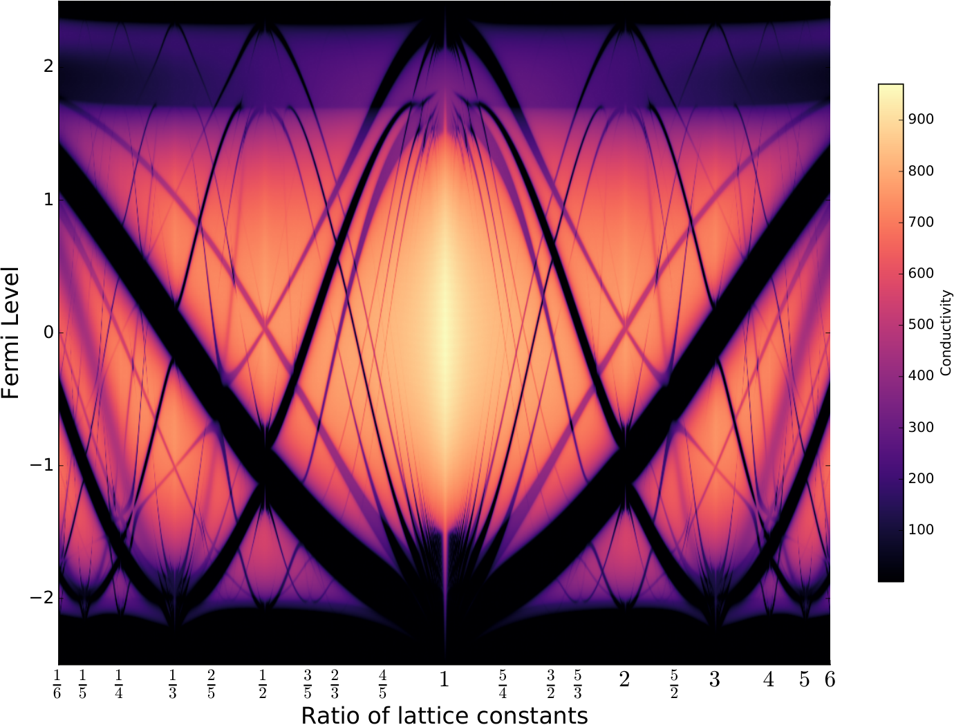
Refer to caption
Figure 7: Conductivity in color scale as a function of Fermi level and lattice constants ratios, with parameter choice W=.5W=.5, σ=.25\sigma=.25, β=τ=250\beta=\tau=250.
Refer to caption
Figure 8: Conductivity in color scale as a function of the integrated density of states.

Next, we plot the conductivity as a function of lattice constants ratio α\alpha and Fermi level μ\mu in Figure 7. The same fractal pattern emerges, however a striking difference is that the conductivity drops at the edges of the gaps (where the density of states is maximum). Strong insulating gaps occur along the spectral gaps as expected, forming a strong fan structure around α=1\alpha=1.

This fan structure is repeated at a number of values of α\alpha corresponding to rational numbers: 1/51/5 and 55, 1/31/3 and 33 are particularly strong, with weaker features at 1/41/4 and 44, 1/21/2 and 22, 3/53/5 and 5/35/3. In general, features such as gaps opening or closing appear at rational values of α\alpha.

Finally, we plot in Figure 8 the conductivity again, which we plot this time as a function of the integrated density of states

nα​(E)=∫−∞Ed​μα,n^{\alpha}(E)=\int_{-\infty}^{E}\mathrm{d}\mu^{\alpha},

where d​μα\mathrm{d}\mu^{\alpha} is the density of states measure defined by (51). The function E↦nα​(E)E\mapsto n^{\alpha}(E) is increasing from 00 to 11, but stays constant in a gap of the spectrum, thus in this representation the size of the insulating gaps is narrowed. Note that in experiments, the control is over the number of electrons per unit cell through gating or doping [21], corresponding to the integrated density of states, and not directly over the Fermi level in general.

Surprisingly, the gaps are still clearly visible in this rescaled presentation, but appear as straight lines. This feature is reminiscent of experimental images of magneto-transport data in small twist angle bilayer graphene [5], leading to exciting perspectives for the application of the framework presented in this paper to more realistic 2D multilayer systems.

5 Acknowledgments

This work was supported in part by ARO MURI Award W911NF-14-1-0247. EC and PC are grateful to Jean Bellissard for useful discussions.

References

  • [1] W. Arveson. A short course on spectral theory, volume 209. Springer Science & Business Media, 2006.
  • [2] J. Bellissard. Coherent and dissipative transport in aperiodic solids. In Lecture Notes in Physics, volume 597, pages 413–486. Springer, 2003.
  • [3] J. Bellissard, A. van Elst, and H. Schulz-Baldes. The noncommutative geometry of the quantum Hall effect. Journal of Mathematical Physics, 35(10):5373–5451, 1994.
  • [4] J. Bezanson, S. Karpinski, V. B. Shah, and A. Edelman. Julia: A fast dynamic language for technical computing. arXiv e-print arXiv:1209.5145, 2012.
  • [5] Y. Cao, J. Y. Luo, V. Fatemi, S. Fang, J. D. Sanchez-Yamagishi, K. Watanabe, T. Taniguchi, E. Kaxiras, and P. Jarillo-Herrero. Superlattice-induced insulating states and valley-protected orbits in twisted bilayer graphene. Physical Review Letters, 117(11):116804, 2016.
  • [6] S. Carr, D. Massatt, P. Cazeaux, S. Fang, M. Luskin, and E. Kaxiras. Twistronics: Manipulating the electronic properties of two-dimensional layered structures through their twist angle. arXiv preprint arXiv:1611.00649, 2016.
  • [7] A. H. Castro Neto, F. Guinea, N. M. R. Peres, K. S. Novoselov, and A. K. Geim. The electronic properties of graphene. Rev. Mod. Phys., 81:109–162, January 2009.
  • [8] P. Cazeaux, M. Luskin, and E. B. Tadmor. Analysis of rippling in incommensurate one-dimensional coupled chains. to appear in Multiscale Modeling and Simulation, June 2016.
  • [9] M. Einsiedler and T. Ward. Ergodic Theory: with a view towards Number Theory. Graduate Texts in Mathematics. Springer London, 2010.
  • [10] S. Fang and E. Kaxiras. Electronic structure theory of weakly interacting bilayers. Physical Review B, 93(23):235153, June 2016.
  • [11] S. Fang, R. Kuate Defo, S. N. Shirodkar, S. Lieu, G. A. Tritsaris, and E. Kaxiras. Ab initio tight-binding hamiltonian for transition metal dichalcogenides. Physical Review B, 92(20):205108, November 2015.
  • [12] A. K. Geim and I. V. Grigorieva. Van der Waals heterostructures. Nature, 499(7459):419–25, July 2013.
  • [13] D. R. Hofstadter. Energy levels and wave functions of bloch electrons in rational and irrational magnetic fields. Physical Review B, 14:2239–2249, September 1976.
  • [14] E. Kaxiras. Atomic and Electronic Structure of Solids. Cambridge University Press, Cambridge, 2003.
  • [15] W. Kohn. Analytic properties of Bloch waves and Wannier functions. Physical Review, 115(4):809, 1959.
  • [16] N. Marzari and D. Vanderbilt. Maximally localized generalized Wannier functions for composite energy bands. Physical review B, 56(20):12847, 1997.
  • [17] D. Massatt, M. Luskin, and C. Ortner. Electronic density of states for incommensurate layers. arXiv preprint arxiv:1608.01968, August 2016.
  • [18] E. Prodan. Quantum transport in disordered systems under magnetic fields: A study based on operator algebras. Applied Mathematics Research eXpress, 2013(2):176–265, 2013.
  • [19] E. Prodan and J. Bellissard. Mapping the current–current correlation function near a quantum critical point. Annals of Physics, 368:1–15, 2016.
  • [20] H Schulz-Baldes and J Bellissard. A kinetic theory for quantum transport in aperiodic media. Journal of Statistical Physics, 91(5-6):991–1026, 1998.
  • [21] K. Sugawara, K. Kanetani, T. Sato, and T. Takahashi. Fabrication of Li-intercalated bilayer graphene. AIP Advances, 1(2), 2011.
  • [22] H. Terrones and M. Terrones. Bilayers of transition metal dichalcogenides: Different stackings and heterostructures. Journal of Materials Research, 29:373–382, 2 2014.
  • [23] G. A. Tritsaris, S. N. Shirodkar, E. Kaxiras, P. Cazeaux, M. Luskin, P. Plecháč, and E. Cancès. Perturbation theory for weakly coupled two-dimensional layers. Journal of Materials Research, 31:959–966, 4 2016.
  • [24] G. H Wannier. The structure of electronic excitation levels in insulating crystals. Physical Review, 52(3):191, 1937.
  • [25] A. Weiße, G. Wellein, A. Alvermann, and H. Fehske. The kernel polynomial method. Reviews of Modern Physics, 78:275–306, Mar 2006.

*