跳到论文正文
W Papers独立论文阅读器 arXiv:1611.08028 论文正文 计算阅读时间 · 0%
引用这篇论文根据当前论文元数据生成,正式投稿前建议核对。


License: arXiv.org perpetual non-exclusive license
arXiv:1611.08028v2 [math.NA] 01 Dec 2017

A fast and spectrally convergent algorithm for rational-order fractional integral and differential equations

Nicholas Hale ††thanks: Department of Mathematical Sciences, Stellenbosch University, Stellenbosch, 7602, South Africa. (nickhale@sun.ac.za)    Sheehan Olver ††thanks: Department of Mathematics, Imperial College, London, SW7 2AZ, United Kingdom (s.olver@imperial.ac.uk)
Abstract

A fast algorithm (linear in the degrees of freedom) for the solution of linear variable-coefficient rational-order fractional integral and differential equations is described. The approach is related to the ultraspherical method for ordinary differential equations [27], and involves constructing two different bases, one for the domain of the operator and one for the range of the operator. The bases are constructed from direct sums of suitably weighted ultraspherical or Jacobi polynomial expansions, for which explicit representations of fractional integrals and derivatives are known, and are carefully chosen so that the resulting operators are banded or almost-banded. Geometric convergence is demonstrated for numerous model problems when the variable coefficients and right-hand side are sufficiently smooth.

keywords
Fractional derivative, spectral method, Ultraspherical polynomials, Jacobi polynomials, Riemann–Liouville, Caputo, Bagley–Torvik
AMS
26A33, 34A08, 65L99

1 Introduction

Fractional derivatives and fractional differential equations (FDEs) are becoming increasingly prevalent in the mathematical modelling of biological and physical processes [10, 17, 21, 22, 24, 29, 32, 33, 34]. Numerical techniques for computing solutions are typically based on finite differences [9, 23, 42] or finite elements [11, 14, 20], but these usually provide only low accuracy solutions due to the global nature of fractional derivatives. There have been some recent developments in spectral methods for FDEs [7, 19, 43], but these are only observed to achieve spectral accuracy for special solutions.

This paper concerns the numerical solution of linear equations involving rational-order fractional integrals and derivatives on the interval [−1,1][-1,1].11 1 Problems defined on any other bounded interval may be mapped to [−1,1][-1,1] by a suitable affine transformation. For p,q∈ℕp,q\in\mathbb{N} with 0<p<q0<p<q, the left-sided p/qp/q-integral is defined as [31]22 2 The right-sided rational-integral, 𝒬1p/qx\prescript{}{x}{\mathcal{Q}^{p/q}_{1}}, is similar, but with the limits on the integral changed from [−1,x][-1,x] to [x,1][x,1] and the bracketed term in the denominator of the integrand negated. Without loss of generality, we focus on the left-sided case.

𝒬xp/q−1​f​(x)=1Γ⁡(p/q)​∫−1xf⁡(t)(x−t)1−p/q​𝑑t,\prescript{}{-1}{{\mathcal{Q}}^{p/q}_{x}}f(x)=\frac{1}{\Gamma(p/q)}\int_{-1}^{x}\frac{f(t)}{(x-t)^{1-p/q}}\,dt, (1)

and for m∈ℕm\in\mathbb{N}, (m+p/q)(m+{p/q})-order derivatives of Riemann–Liouville (RL) and Caputo types are given by

𝒟xm+p/q−1R​L​f​(x)=dm+1d​xm+1​(𝒬1−p/qx−1​f​(x)) and𝒟xm+p/q−1C​f​(x)=𝒬1−p/qx−1​(dm+1d​xm+1​f​(x)),\prescript{RL\!}{-1}{\mathcal{D}}_{x}^{m+p/q}f(x)=\frac{d^{m+1}}{dx^{m+1}}\left(\prescript{}{-1}{\mathcal{Q}}_{x}^{1-p/q}f(x)\right)\quad\text{ and}\quad\prescript{C\!}{-1}{\mathcal{D}}^{m+p/q}_{x}f(x)=\prescript{}{-1}{\mathcal{Q}}_{x}^{1-p/q}\left(\frac{d^{m+1}}{dx^{m+1}}f(x)\right), (2)

respectively. We propose an approach which achieves spectral convergence in linear complexity for a broad class of linear fractional integral equations (FIEs) and FDEs composed of such rational-order operators. We demonstrate the accuracy and flexibility of the method on numerous examples, such as in Figure 9 where we solve the generalised second-kind Abel integral equation

u⁡(x)+λ​∫−1xu⁡(t)(x−t)1/3=f⁡(x),\displaystyle u(x)+\lambda\int_{-1}^{x}\frac{u(t)}{(x-t)^{1/3}}=f(x), x∈[−1,1],\displaystyle\qquad x\in[-1,1], (3)

and in Figure 11, where we solve a highly-oscillatory fractional Airy equation

i3/2​Dx3/2−1R​L​u​(x)−104​x​u​(x)=0,\displaystyle i^{3/2}\prescript{RL}{-1}{D^{3/2}_{x}}u(x)-10^{4}xu(x)=0, x∈[−1,1],u⁡(−1)=0,u⁡(1)=1.\displaystyle\qquad x\in[-1,1],\qquad u(-1)=0,\ u(1)=1. (4)

The approach is related to the ultraspherical spectral (US) method for ordinary differential equations [27] and singular integral equations [35], where the key idea is that the underlying operators are banded when represented by their action on appropriately chosen bases, built out of ultraspherical polynomials. Here, for integral equations, the idea is similar: we exploit the fact that fractional integration is a banded operator between a suitable direct sum space formed of qq weighted Jacobi polynomial bases (which can be related to the “generalised Jacobi functions” of [7] and “polyfractinomials” of [43]), for which an explicit representation of the fractional derivative is available. However, a critical difficulty arises for differential equations: the bases are not compatible, in the sense that the weights in the range of the operators differ from those of the domain. To overcome this difficulty we expand the solution as a direct sum of weighted Jacobi polynomials as before, but then consider another basis formed as a direct sum of qq different weighted Jacobi polynomial bases to represent the range of the operator (for a total of 2qq bases).33 3 When q=2q=2 the integral in (1) is called the left-sided half-integral, and we shall see below that more elegant formulae can be obtained in this instance using ultraspherical rather than Jacobi polynomials. If these two direct sum spaces are chosen appropriately, then the resulting operators are banded.

There have been two recent additions to the literature which also provide spectral accuracy for FDEs, namely the works of Zayernouri and Karniadakis [43] and Chen, Shen, and Wang [7].44 4 There has also been recent work in spectral methods for tempered fractional differential equations (see, for example, [44]), but it is not clear that these approaches provide spectral accuracy in the limit α→0\alpha\rightarrow 0, i.e., the non-tempered case. The foundation of both is the same formula for the fractional integral of weighted Jacobi polynomials (i.e., [2, Theorem 6.72(b)]) which also forms the basis of our own approach (see Theorems 1 and 7.15 below). Whereas in this paper we limit our attention to rational-order derivatives, both [7] and [43] deal with arbitrary orders, and so are in a sense more general. However, the algorithm proposed by Zayernouri and Karniadakis is collocation based, leading to dense matrices and 𝒪⁡(N3){\cal{O}}(N^{3}) complexity. Spectral accuracy is demonstrated for a few select problems, but it is typically sub-geometric. Furthermore, the discussion is limited to zero Dirichlet boundary conditions. The algorithm of Chen, Shen, and Wang has linear complexity, but applies only to FDEs of the form 𝒟xν−1​u​(x)=f⁡(x){}_{-1}{\cal D}^{\nu}_{x}u(x)=f(x) and 𝒟1νx​u​(x)=f⁡(x){}_{x}{\cal D}^{\nu}_{1}u(x)=f(x) (for both RL and Caputo definitions). In this work we shall consider FDEs which are linear combinations of rational-integer order derivatives with more general boundary conditions and demonstrate geometric convergence with linear complexity.

The bulk of this paper is dedicated to introducing the proposed algorithm specifically for the case of half-integral order integrals and derivatives (i.e., p=1p=1 and q=2q=2 in (1) and (2)), for which the approach and derivation are more intuitive to follow. However, the extension to more general rational-order derivatives and integrals follows readily once the approach is understood for the half-integer order case, and in the penultimate section we describe in some detail how this is achieved and give further examples. As such, the outline of this paper is as follows. In Section 2 we introduce some necessary preliminaries regarding ultraspherical polynomials, in particular an explicit formula for their half-integrals and various transformations between different weighted ultraspherical polynomial expansions. In Sections 3–5 we use these to derive a fast and geometrically convergent algorithm for a certain class of half-integer order FIEs and FDEs of Riemann–Liouville and Caputo type, respectively. Section 6 discusses some computational issues relating to these algorithms, such as the efficient computation of the required polynomial coefficients and solution of the linear systems describing the FIEs/FDEs. In Section 7 we describe how the ideas of the previous sections may be adapted to consider more general rational-order FIEs, before concluding in Section 8 with one final example and some suggestions for future work.

Remark: The experiments in this paper were conducted in MATLAB (code to reproduce all figures is available online at [15]), and a Julia implementation of the algorithm is available in ApproxFun.jl [26].

2 Preliminaries

In this section we consider the required preliminaries needed for working with half-integrals

𝒬x1/2−1​f​(x)=1π​∫−1xf⁡(t)(x−t)1/2​𝑑t,\prescript{}{-1}{{\mathcal{Q}}^{1/2}_{x}}f(x)=\frac{1}{\sqrt{\pi}}\int_{-1}^{x}\frac{f(t)}{(x-t)^{1/2}}\,dt, (5)

and half-integer order derivatives

𝒟xm+1/2−1R​L​f​(x)=dm+1d​xm+1​(𝒬1/2x−1​f​(x)) and𝒟xm+1/2−1C​f​(x)=𝒬1/2x−1​(dm+1d​xm+1​f​(x)),m∈ℕ.\prescript{RL\!}{-1}{\mathcal{D}}_{x}^{m+1/2}f(x)=\frac{d^{m+1}}{dx^{m+1}}\left(\prescript{}{-1}{\mathcal{Q}}_{x}^{1/2}f(x)\right)\quad\text{ and}\quad\prescript{C\!}{-1}{\mathcal{D}}^{m+1/2}_{x}f(x)=\prescript{}{-1}{\mathcal{Q}}_{x}^{1/2}\left(\frac{d^{m+1}}{dx^{m+1}}f(x)\right),\quad m\in\mathbb{N}. (6)

Our primary tools here are ultraspherical polynomials, specifically Legendre and Chebyshev polynomials, as described below.

Remark: We shall see in Section 7 that in the case of general rational-order integrals and derivatives one must instead work with Jacobi polynomials. Whilst it is possible to unify these approaches and use Jacobi polynomials in the half-order case, we find that using the ultraspherical polynomials here leads to cleaner and more elegant formulae, and so choose to formulate our algorithm with these instead.

2.1 Ultraspherical polynomials

The ultraspherical (or Gegenbauer) polynomials, Cn(λ)​(x)C_{n}^{(\lambda)}(x), are orthogonal with respect to the weight function (1−x2)λ−1/2(1-x^{2})^{\lambda-1/2} on the interval [−1,1][-1,1], where λ>−12\lambda>-{1\over 2} and λ≠0\lambda\neq 0. For any λ>0\lambda>0 the degree nn ultraspherical polynomial may be defined via the recurrence [12, 18.9.1]

C−1(λ)​(x)=0,C0(λ)​(x)=1,(n+1)​Cn+1(λ)​(x)=2​(n+λ)​x​Cn(λ)​(x)−(n+2​λ−1)​Cn−1(λ)​(x).C_{-1}^{(\lambda)}(x)=0,\quad C_{0}^{(\lambda)}(x)=1,\quad(n+1)C^{(\lambda)}_{n+1}(x)=2(n+\lambda)xC^{(\lambda)}_{n}(x)-(n+2\lambda-1)C^{(\lambda)}_{n-1}(x). (7)

The Legendre polynomials, Pn​(x)P_{n}(x), and the second-kind Chebyshev polynomials, Un​(x)U_{n}(x), are special cases of the ultraspherical polynomials with λ=12\lambda=\frac{1}{2} and λ=1\lambda=1, respectively. These two will be of particular importance in our algorithms described in Sections 3–5 for half-integer order FIEs and FDEs.

For any x∈ℂx\in\mathbb{C}, λ>0\lambda>0, and γ∈ℝ\gamma\in\mathbb{R}, we define 𝐂γ(λ)​(x)\mathbf{C}^{(\lambda)}_{\gamma}(x) as the quasimatrix — a ‘matrix’ whose ‘columns’ are functions defined on an interval [36] — whose jjth column is the degree (j−1)(j-1)th ultraspherical polynomial with parameter λ\lambda weighted by (1+x)γ(1+x)^{\gamma}, i.e.,

𝐂γ(λ)​(x):=[(1+x)γ​C0(λ)​(x),(1+x)γ​C1(λ)​(x),…].\mathbf{C}^{(\lambda)}_{\gamma}(x):=\Big[(1+x)^{\gamma}C_{0}^{(\lambda)}(x),\,\,(1+x)^{\gamma}C_{1}^{(\lambda)}(x),\,\,\dots\Big]. (8)

We refer to these as weighted ultraspherical bases and note that the columns of 𝐂γ(λ)​(x)\mathbf{C}^{(\lambda)}_{\gamma}(x) are related to the “generalised Jacobi functions” of [7] and “polyfractinomials” of [43]. With each such basis (8) we may associate a space of coefficients, 𝐂γ(λ)≅ℂ∞\mathbf{C}^{(\lambda)}_{\gamma}\cong\mathbb{C}^{\infty}, and if u¯=(u0,u1,…)⊤∈𝐂γ(λ)\underline{u}={{\left({u_{0},u_{1},\ldots}\right)}^{\top}}\in\mathbf{C}^{(\lambda)}_{\gamma} such that

∑k=0∞|uk|​sup−1≤x≤1|Ck(λ)​(x)|=∑k=0∞|uk|​Γ⁡(2​λ+k)Γ⁡(2​λ)​k!<∞,\sum_{k=0}^{\infty}\left|{u_{k}}\right|\sup_{-1\leq x\leq 1}\left|{C_{k}^{(\lambda)}(x)}\right|=\sum_{k=0}^{\infty}\left|{u_{k}}\right|\frac{\Gamma(2\lambda+k)}{\Gamma(2\lambda)k!}<\infty, (9)

then u⁡(x)=𝐂γ(λ)​(x)​u¯u(x)=\mathbf{C}^{(\lambda)}_{\gamma}(x)\underline{u} defines a continuous function away from x=−1x=-1. For convenience, we denote 𝐏γ:=𝐂γ(1/2){\mathbf{P}_{\gamma}}:=\mathbf{C}_{\gamma}^{(1/2)}, 𝐔γ:=𝐂γ(1){\mathbf{U}_{\gamma}}:={\mathbf{C}}^{(1)}_{\gamma}, and 𝐂(λ):=𝐂0(λ){\mathbf{C}}^{(\lambda)}:={\mathbf{C}}_{0}^{(\lambda)}.

Linear operators which can be applied to one such weighted ultraspherical basis and expanded in another induce infinite-dimensional matrices that can be viewed as acting between different 𝐂γ(λ)\mathbf{C}^{(\lambda)}_{\gamma} spaces. For example, given a continuous linear operator ℒ:X→Y{\cal L}:X\rightarrow Y so that (1+x)λ​Ck(λ)​(x)∈X(1+x)^{\lambda}C_{k}^{(\lambda)}(x)\in X and (1+x)c​Cj(ℓ)​(x)∈Y(1+x)^{c}C_{j}^{(\ell)}(x)\in Y with the property

ℒ⁡[(1+⋄)γ​Ck(λ)]​(x)=∑j=k−mk+mLj​k​(1+x)c​Cj(ℓ)​(x),{\cal L}[(1+\diamond)^{\gamma}C_{k}^{(\lambda)}](x)=\sum_{j=k-m}^{k+m}L_{jk}(1+x)^{c}C_{j}^{(\ell)}(x), (10)

we can associate it with an mm-banded (i.e., banded with bandwidth mm) infinite-dimensional matrix

L:=(L00⋯L0​m⋱L1​mL1,m+1Lm​0Lm​1⋱Lm​m⋱Lm+1,1⋱⋱⋱⋱⋱⋱).L:=\begin{pmatrix}L_{00}&\cdots&L_{0m}\vphantom{\frac{1+2\lambda}{2+\lambda}\ddots}\cr\vdots&\ddots&L_{1m}&L_{1,m+1}\vphantom{\frac{1+2\lambda}{2+\lambda}\ddots}\cr L_{m0}&L_{m1}&\ddots&L_{mm}&\ddots\cr&L_{m+1,1}&\ddots&\ddots&\ddots\cr&&\ddots&\ddots&\ddots\end{pmatrix}. (11)

Since LL is banded, multiplication is a well-defined operation on ℂ∞\mathbb{C}^{\infty} and (11) can be viewed as an operator L:𝐂γ(λ)→𝐂c(ℓ)L:\mathbf{C}^{(\lambda)}_{\gamma}\rightarrow\mathbf{C}_{c}^{(\ell)}. To relate the operator LL and the operator ℒ{\cal L} we note that, by construction, we have55 5 Here and throughout we use ⋄\diamond to represent the dummy variable in an operator.

ℒ⁡[(1+⋄)γ​Ck(λ)]​(x)=ℒ​𝐂γ(λ)​(x)​e¯k=𝐂c(ℓ)​(x)​L​e¯k.{\cal L}[(1+\diamond)^{\gamma}C_{k}^{(\lambda)}](x)={\cal L}\mathbf{C}^{(\lambda)}_{\gamma}(x)\underline{e}_{k}=\mathbf{C}^{(\ell)}_{c}(x)L\underline{e}_{k}. (12)

If u⁡(x)∈Xu(x)\in X, then, assuming that the 𝐂γ(λ)​(x)​e¯k\mathbf{C}^{(\lambda)}_{\gamma}(x)\underline{e}_{k} are dense in XX, there exists u¯∈𝐂γ(λ)\underline{u}\in\mathbf{C}^{(\lambda)}_{\gamma} so that u⁡(x)=𝐂γ(λ)​(x)​u¯u(x)=\mathbf{C}^{(\lambda)}_{\gamma}(x)\underline{u}. Because ℒ{\cal L} is continuous, we have

ℒ​u=ℒ​𝐂γ(λ)​(x)​u¯=𝐂c(ℓ)​(x)​L​u¯,{\cal L}u={\cal L}\mathbf{C}^{(\lambda)}_{\gamma}(x)\underline{u}=\mathbf{C}^{(\ell)}_{c}(x)L\underline{u}, (13)

and therefore applying LL to u⁡(x)u(x) is equivalent to applying ℒ{\cal L} to u¯\underline{u}.

The US method [27] for differential equations requires three such banded operators which act on ultraspherical polynomials: conversion, multiplication, and differentiation. We now revisit these operators in the case of weighted ultraspherical polynomials and introduce new operators corresponding to fractional integration and fractional differentiation of half-integer order.

Remark: In Sections 3–5 we will seek solutions to FIEs and FDEs formed as linear combinations of Legendre polynomials, Pn​(x)P_{n}(x), and weighted Chebyshev polynomials of the second kind, 1+x​Un​(x)\sqrt{1+x}U_{n}(x). Another possibility is to choose a direct sum of Legendre polynomials and weighted Chebyshev polynomials of the first kind, Tn​(x)/1+xT_{n}(x)/\sqrt{1+x} (for which one can also find explicit and compact formulae for half-integer order integrals and derivatives). We make the decision to use second-kind polynomials for the following reasons: Firstly, Tn​(x)T_{n}(x) is not an ultraspherical polynomial. In particular, this means that the formulae involving Tn​(x)T_{n}(x) in the next few sections must be treated separately from Cn(λ)​(x)C_{n}^{(\lambda)}(x), which greatly clutters the exposition. Secondly, in most applications of interest the solution remains finite, so a basis which remains bounded in the computational interval is preferred. (See also the remark in Section 4.1.)

2.2 Conversion operators

We consider two representations of the identity operator, ℐ\mathcal{I}, which map between different 𝐂γ(λ)\mathbf{C}^{(\lambda)}_{\gamma} spaces. First, the relationship [12, 18.9.7]

Cn(λ)​(x)=λn+λ​(Cn(λ+1)​(x)−Cn−2(λ+1)​(x)),C^{(\lambda)}_{n}(x)=\frac{\lambda}{n+\lambda}\big(C^{(\lambda+1)}_{n}(x)-C^{(\lambda+1)}_{n-2}(x)\big), (14)

induces operators Sλ:𝐂γ(λ)→𝐂γ(λ+1)S_{\lambda}:\mathbf{C}^{(\lambda)}_{\gamma}\rightarrow\mathbf{C}^{(\lambda+1)}_{\gamma} defined by

Sλ:=(10−λλ+2λλ+10−λλ+3λλ+20−λλ+4⋱⋱⋱),S_{\lambda}:=\begin{pmatrix}1&0&\!\frac{-\lambda}{\lambda+2}\cr&\!\frac{\lambda}{\lambda+1}&0&\!\frac{-\lambda}{\lambda+3}\cr&&\!\frac{\lambda}{\lambda+2}&0&\!\frac{-\lambda}{\lambda+4}\cr&&&\!\ddots&\ddots&\!\ddots\end{pmatrix}, (15)

so that if u¯∈𝐂γ(λ)\underline{u}\in\mathbf{C}^{(\lambda)}_{\gamma} then u⁡(x)=𝐂γ(λ)​(x)​u¯=𝐂γ(λ+1)​Sλ​u¯u(x)=\mathbf{C}^{(\lambda)}_{\gamma}(x)\underline{u}=\mathbf{C}^{(\lambda+1)}_{\gamma}S_{\lambda}\underline{u}. These are precisely the conversion operators 𝒮λ{\cal{S}_{\lambda}} as described in [27]. Here, and in the other operators that follow, when SS is acting on either 𝐏\mathbf{P} or 𝐔\mathbf{U}, we shall subscript with these, rather than the corresponding value of λ\lambda. That is,

S𝐏:=S1/2=(10−15130−17150⋱⋱⋱)and S𝐔:=S1=(10−13120−14130⋱⋱⋱).S_{\mathbf{P}}:=S_{1/2}=\begin{pmatrix}1&0&-\frac{1}{5}\cr&\frac{1}{3}&0&-\frac{1}{7}\vphantom{\ddots}\cr&&\frac{1}{5}&0&\ddots\cr&&&\!\ddots&\ddots\end{pmatrix}\quad\text{and }\quad S_{\mathbf{U}}:=S_{1}=\begin{pmatrix}1&0&-\frac{1}{3}\cr&\frac{1}{2}&0&-\frac{1}{4}\vphantom{\ddots}\cr&&\frac{1}{3}&0&\ddots\cr&&&\!\ddots&\ddots&\end{pmatrix}. (16)

A second relationship

(1+x)​Cn(λ)​(x)=n+12​(n+λ)​Cn+1(λ)​(x)+Cn(λ)​(x)+n+2​λ−12​(n+λ)​Cn−1(λ)​(x),λ>0,(1+x)C^{(\lambda)}_{n}(x)=\frac{n+1}{2(n+\lambda)}C^{(\lambda)}_{n+1}(x)+C^{(\lambda)}_{n}(x)+\frac{n+2\lambda-1}{2(n+\lambda)}C^{(\lambda)}_{n-1}(x),\qquad\lambda>0, (17)

which can be readily derived from the recurrence relations (7), induces operators Rλ:𝐂γ(λ)→𝐂γ−1(λ)R_{\lambda}:\mathbf{C}^{(\lambda)}_{\gamma}\rightarrow\mathbf{C}^{(\lambda)}_{\gamma-1}, where

Rλ:=12​(22​λ1+λ1λ21+2​λ2+λ21+λ22+2​λ3+λ32+λ2⋱⋱⋱),R_{\lambda}:=\frac{1}{2}\begin{pmatrix}2&\frac{2\lambda}{1+\lambda}\cr\frac{1}{\lambda}&2&\!\frac{1+2\lambda}{2+\lambda}\vphantom{\ddots}\cr&\!\frac{2}{1+\lambda}&2&\!\frac{2+2\lambda}{3+\lambda}\vphantom{\ddots}\cr&&\!\frac{3}{2+\lambda}&2&\ddots\cr&&&\!\ddots&\!\ddots\end{pmatrix}, (18)

So that if u¯∈𝐂γ(λ)\underline{u}\in\mathbf{C}^{(\lambda)}_{\gamma} then u⁡(x)=𝐂γ(λ)​(x)​u¯=𝐂γ−1(λ)​Rλ​u¯u(x)=\mathbf{C}^{(\lambda)}_{\gamma}(x)\underline{u}=\mathbf{C}^{(\lambda)}_{\gamma-1}R_{\lambda}\underline{u}. Note in particular that R𝐔R_{\mathbf{U}} has the simple form

R𝐔:=R1=12​(2112⋱⋱⋱).R_{\mathbf{U}}:=R_{1}=\frac{1}{2}\begin{pmatrix}2&1\cr 1&2&\ddots\vphantom{\ddots}\cr&\!\ddots&\!\ddots\end{pmatrix}. (19)

2.3 Multiplication operators

As outlined in [35] and [40], polynomial multiplication can be viewed as a banded operator acting on 𝐂(λ)\mathbf{C}^{(\lambda)} spaces. In particular, the basic building block is the Jacobi operator, built out of the three-term recurrence (7):

x​Cn(λ)​(x)=n+12​(n+λ)​Cn+1(λ)​(x)+n+2​λ−12​(n+λ)​Cn−1(λ)​(x).xC_{n}^{(\lambda)}(x)=\frac{n+1}{2(n+\lambda)}C_{n+1}^{(\lambda)}(x)+\frac{n+2\lambda-1}{2(n+\lambda)}C_{n-1}^{(\lambda)}(x). (20)

In the language of Section 2.1, this amounts to choosing ℒ=x{\cal L}=x, inducing the operator Jλ:𝐂γ(λ)→𝐂γ(λ)J_{\lambda}:\mathbf{C}^{(\lambda)}_{\gamma}\rightarrow\mathbf{C}^{(\lambda)}_{\gamma} defined as

Jλ:=12​(02​λ1+λ1λ01+2​λ2+λ21+λ02+2​λ3+λ32+λ0⋱⋱⋱),J_{\lambda}:=\frac{1}{2}\begin{pmatrix}0&\frac{2\lambda}{1+\lambda}\cr\frac{1}{\lambda}&0&\!\frac{1+2\lambda}{2+\lambda}\cr&\!\frac{2}{1+\lambda}&0&\!\frac{2+2\lambda}{3+\lambda}\cr&&\!\frac{3}{2+\lambda}&0&\ddots\cr&&&\!\ddots&\!\ddots\end{pmatrix}, (21)

so that if u¯∈𝐂γ(λ)\underline{u}\in\mathbf{C}^{(\lambda)}_{\gamma} then x​u​(x)=x​𝐂γ(λ)​(x)​u¯=𝐂γ(λ)​Jλ​u¯xu(x)=x\mathbf{C}^{(\lambda)}_{\gamma}(x)\underline{u}=\mathbf{C}^{(\lambda)}_{\gamma}J_{\lambda}\underline{u}. If Cn(ℓ)​(x)C^{(\ell)}_{n}(x) is another ultraspherical polynomial then its corresponding three-term recurrence applied to JλJ_{\lambda} gives

Cn+1(ℓ)​(Jλ)=2​n+ℓn+1​Jλ​Cn(ℓ)​(Jλ)−n+2​ℓ−1n+1​Cn−1(ℓ)​(Jλ),n≥1C^{(\ell)}_{n+1}(J_{\lambda})=2\frac{n+\ell}{n+1}J_{\lambda}C^{(\ell)}_{n}(J_{\lambda})-\frac{n+2\ell-1}{n+1}C^{(\ell)}_{n-1}(J_{\lambda}),\qquad n\geq 1 (22)

with C−1(ℓ)​(Jλ)=0C^{(\ell)}_{-1}(J_{\lambda})=0, C0(ℓ)​(Jλ)=1C^{(\ell)}_{0}(J_{\lambda})=1, and the multiplication operator Πλ​[Cn(ℓ)]:𝐂γ(λ)→𝐂γ(λ)\Pi_{\lambda}[C^{(\ell)}_{n}]:\mathbf{C}^{(\lambda)}_{\gamma}\rightarrow\mathbf{C}^{(\lambda)}_{\gamma} may be defined recursively as

Πλ​[Cn+1(ℓ)]=2​n+ℓn+1​Jλ​Πλ​[Cn(ℓ)]−n+2​ℓ−1n+1​Πλ​[Cn−1(ℓ)],n≥1\Pi_{\lambda}[C^{(\ell)}_{n+1}]=2\frac{n+\ell}{n+1}J_{\lambda}\Pi_{\lambda}[C^{(\ell)}_{n}]-\frac{n+2\ell-1}{n+1}\Pi_{\lambda}[C^{(\ell)}_{n-1}],\qquad n\geq 1 (23)

where Πλ​[C−1(ℓ)]=0\Pi_{\lambda}[C^{(\ell)}_{-1}]=0 and Πλ​[C0(ℓ)]=I\Pi_{\lambda}[C^{(\ell)}_{0}]=I. Each term in the recursion will increase by the bandwidth by 1 (since JλJ_{\lambda} has bandwidth 1), so Πλ​[Cd(ℓ)]\Pi_{\lambda}[C^{(\ell)}_{d}] is banded with bandwidth dd. Then, by linearity of Πλ\Pi_{\lambda} and the orthogonality of ultraspherical polynomials, given any degree dd polynomial pp we may construct

Πλ[p(x)=∑n=0dpnCn(ℓ)(x)]=∑n=0dpnΠλ[Cn(ℓ)],\Pi_{\lambda}\Big[p(x)=\sum_{n=0}^{d}p_{n}C_{n}^{(\ell)}(x)\Big]=\sum_{n=0}^{d}p_{n}\Pi_{\lambda}[C_{n}^{(\ell)}], (24)

which also has bandwidth dd and satisfies p⁡(x)​u​(x)=p⁡(x)​𝐂γ(λ)​(x)​u¯=𝐂γ(λ)​(x)​Πλ​[p⁡(x)]​u¯p(x)u(x)=p(x)\mathbf{C}^{(\lambda)}_{\gamma}(x)\underline{u}=\mathbf{C}^{(\lambda)}_{\gamma}(x)\Pi_{\lambda}[p(x)]\underline{u} when u¯∈𝐂γ(λ)\underline{u}\in\mathbf{C}^{(\lambda)}_{\gamma}.

One may take ℓ=λ\ell=\lambda, in which case the columns of Πλ​[Cd(λ)]\Pi_{\lambda}[C_{d}^{(\lambda)}] give rise to linearisation formulae for products of the form Cd(λ)​(x)​Cn(λ)​(x)C_{d}^{(\lambda)}(x)C_{n}^{(\lambda)}(x) [12, 18.18.22]. Alternatively, one can construct a similar recurrence relationship based on Chebyshev polynomials of the first kind, in which case

Πλ​[Tn+1]=2​Jλ​Πλ​[Cn(ℓ)]−Πλ​[Tn−1],n>1,\Pi_{\lambda}[T_{n+1}]=2J_{\lambda}\Pi_{\lambda}[C^{(\ell)}_{n}]-\Pi_{\lambda}[T_{n-1}],\qquad n>1, (25)

with Πλ​[T0]=1\Pi_{\lambda}[T_{0}]=1, Πλ​[T1]=x\Pi_{\lambda}[T_{1}]=x, and

Πλ[p(x)=∑n=0dpnTn(x)]=∑n=0dpnΠλ[Tn].\Pi_{\lambda}\Big[p(x)=\sum_{n=0}^{d}p_{n}T_{n}(x)\Big]=\sum_{n=0}^{d}p_{n}\Pi_{\lambda}[T_{n}]. (26)

Since Chebyshev coefficients of a polynomial are readily computed by a discrete cosine transform, this can often be more convenient than (23). When pp is not a polynomial but a sufficiently differentiable function, we can approximate it to high accuracy by a polynomial. In particular, if pp is analytic in some neighbourhood of [−1,1][-1,1], then the polynomial approximation will converge geometrically, and the degree of the approximant (and hence bandwith of Πλ\Pi_{\lambda}) will typically be small [39].

2.4 Integral operators

The foundation of our approach is the following formula, which shows how the half-integral of certain weighted ultraspherical polynomials may be computed in closed form:

Theorem 1.

For any λ>0,n≥0\lambda>0,n\geq 0,

−1𝒬x1/2[(1+⋄)λ−1/2Cn(λ)](x)=Γ⁡(λ+1/2)Γ​(λ)​(n+λ)(1+x)λ(Cn(λ+1/2)(x)−Cn−1(λ+1/2)(x)),_{-1}\mathcal{Q}_{x}^{1/2}[(1+\diamond)^{\lambda-1/2}C^{(\lambda)}_{n}](x)=\frac{\Gamma(\lambda+1/2)}{\Gamma(\lambda)(n+\lambda)}(1+x)^{\lambda}\big(C_{n}^{(\lambda+1/2)}(x)-C_{n-1}^{(\lambda+1/2)}(x)\big), (27)
Proof.

Follows from relating Cn(λ)​(x)C_{n}^{(\lambda)}(x) to the Jacobi polynomial Pn(λ−1/2,λ−1/2)​(x)P_{n}^{(\lambda-1/2,\lambda-1/2)}(x) and using the closed form expression for fractional integrals of weighted Jacobi polynomials [2, Theorem 6.72(b)]. Applying the symmetric version of [12, 18.9.5] to the right-hand side and converting Pn(λ,λ)​(x)P^{(\lambda,\lambda)}_{n}(x) back to Cn(λ+1/2)​(x)C^{(\lambda+1/2)}_{n}(x) yields the required result. ∎

Corollary 2.
−1𝒬x1/2Pn(x)=2​1+xπ​(2​n+1)(Un(x)−Un−1(x))_{-1}\mathcal{Q}_{x}^{1/2}P_{n}(x)=\frac{2\sqrt{1+x}}{\sqrt{\pi}(2n+1)}\big({U_{n}(x)-U_{n-1}(x)}\big) (28)

and

−1𝒬x1/2[1+⋄Un](x)=π2(Pn+1(x)+Pn(x))_{-1}\mathcal{Q}_{x}^{1/2}[\sqrt{1+\diamond}U_{n}](x)=\frac{\sqrt{\pi}}{2}\big({P_{n+1}(x)+P_{n}(x)}\big) (29)
Proof.

The first follows immediately from setting λ=1/2\lambda=1/2 in (27). For the second, take λ=1\lambda=1 in (27) and make the observation (see Appendix A) that n⁡(Pn​(x)+Pn−1​(x))=(1+x)​(Cn−1(3/2)​(x)−Cn−2(3/2)​(x))n\big(P_{n}(x)+P_{n-1}(x)\big)=(1+x)\big(C_{n-1}^{(3/2)}(x)-C_{n-2}^{(3/2)}(x)\big). ∎

We may therefore, in the language of Section 2.1, consider half-integration as a banded operator between the spaces of Legendre polynomials and weighted Chebyshev polynomials, and define the associated banded half-integer order integral operators Q𝐏1/2:𝐏→𝐔1/2Q^{1/2}_{\mathbf{P}}:\mathbf{P}\rightarrow\mathbf{U}_{1/2} and Q𝐔1/21/2:𝐔1/2→𝐏Q^{1/2}_{\mathbf{U}_{1/2}}:\mathbf{U}_{1/2}\rightarrow\mathbf{P} as

Q𝐏1/2:=2π​(1−1313−1515⋱⋱)and Q𝐔1/21/2:=π2​(11111⋱⋱),Q^{1/2}_{\mathbf{P}}:=\frac{2}{\sqrt{\pi}}\begin{pmatrix}1&\!-\frac{1}{3}\vphantom{\ddots}&\cr&\!\phantom{-}\frac{1}{3}&-\frac{1}{5}\vphantom{\ddots}&\phantom{-1}\cr&&\phantom{-}\frac{1}{5}\vphantom{\ddots}&\ddots\cr\phantom{\ddots}&\phantom{\ddots}&\phantom{\ddots}&\ddots\end{pmatrix}\quad\text{and }\quad Q^{1/2}_{\mathbf{U}_{1/2}}:=\frac{\sqrt{\pi}}{2}\begin{pmatrix}1\vphantom{\ddots}\cr 1&1\vphantom{\ddots}\cr&1&1\vphantom{\ddots}\cr\phantom{\ddots}&\phantom{\ddots}&\ddots&\ddots\end{pmatrix},\qquad (30)

respectively. Therefore, letting u¯𝐏∈𝐏\underline{u}_{\mathbf{P}}\in\mathbf{P} and u¯𝐔1/2∈𝐔1/2\underline{u}_{\mathbf{U}_{1/2}}\in\mathbf{U}_{1/2} then we have that Qx1/2−1​𝐏​(x)​u¯𝐏=𝐔1/2​(x)​Q𝐏1/2​u¯𝐏{}_{-1}Q^{1/2}_{x}\mathbf{P}(x)\underline{u}_{\mathbf{P}}=\mathbf{U}_{1/2}(x)Q^{1/2}_{\mathbf{P}}\underline{u}_{\mathbf{P}} and Qx1/2−1​𝐔1/2​(x)​u¯𝐔1/2=𝐏⁡(x)​Q𝐔1/21/2​u¯𝐔1/2{}_{-1}Q^{1/2}_{x}\mathbf{U}_{1/2}(x)\underline{u}_{\mathbf{U}_{1/2}}=\mathbf{P}(x)Q^{1/2}_{\mathbf{U}_{1/2}}\underline{u}_{\mathbf{U}_{1/2}}.66 6 Henceforth, we cease (with a few exceptions) to explicitly state such equalities for each operator we introduce. It should be clear from the context which continuous operator is in question, and the range and domain of the discrete operator from the notation introduced in (13).

If we define Q𝐏:=Q𝐔1/21/2​Q𝐏1/2Q_{\mathbf{P}}:=Q^{1/2}_{\mathbf{U}_{1/2}}Q^{1/2}_{\mathbf{P}} so Q𝐏:𝐏→𝐏Q_{\mathbf{P}}:\mathbf{P}\rightarrow\mathbf{P} is given by

Q𝐏=(1−1310−15130−17150⋱⋱⋱),Q_{\mathbf{P}}=\begin{pmatrix}1&-\frac{1}{3}&\vphantom{\ddots}\cr 1&0&-\frac{1}{5}&\vphantom{\ddots}\cr&\frac{1}{3}&0&-\frac{1}{7}&\vphantom{\ddots}\cr\phantom{\ddots}&\phantom{\ddots}&\frac{1}{5}&0&\ddots\cr&&&\ddots&\ddots\end{pmatrix}, (31)

we see that this is consistent with the relation

𝒬1x−1​Pn​(x)=∫−1xPn​(t)​𝑑t={12​n+1​(Pn​(x)−Pn−2​(x)),n≥1,P1​(x)+P0​(x),n=0,{}_{-1}\mathcal{Q}_{x}^{1}P_{n}(x)=\int_{-1}^{x}P_{n}(t)\,dt=\begin{cases}\frac{1}{2n+1}\big(P_{n}(x)-P_{n-2}(x)\big),&n\geq 1,\\ P_{1}(x)+P_{0}(x),&n=0,\end{cases} (32)

for the integral of Legendre polynomials (which can be obtained from [12, 18.16.1] and [12, 18.9.6]). We may go farther and repeatedly combine the Q𝐏Q_{\mathbf{P}} and Q𝐔1/2Q_{\mathbf{U}_{1/2}} operators to define banded operators between the spaces 𝐏\mathbf{P} and 𝐔1/2\mathbf{U}_{1/2} representing integral operators of half-integer order, by repeatedly applying the matrices (30), i.e., 𝒬xm−1{}_{-1}\mathcal{Q}^{m}_{x} and 𝒬xm+1/2−1{}_{-1}\mathcal{Q}^{m+1/2}_{x}. In particular, we have

Q𝐏m+1/2:=Q𝐏1/2​(Q𝐔1/21/2​Q𝐏1/2)m:𝐏→𝐔1/2Q^{m+1/2}_{\mathbf{P}}:=Q^{1/2}_{\mathbf{P}}\big(Q^{1/2}_{\mathbf{U}_{1/2}}Q^{1/2}_{\mathbf{P}}\big)^{m}:\mathbf{P}\rightarrow\mathbf{U}_{1/2} (33)
Q𝐔1/2m+1/2:=Q𝐔1/21/2​(Q𝐏1/2​Q𝐔1/21/2)m:𝐔1/2→𝐏.Q^{m+1/2}_{\mathbf{U}_{1/2}}:=Q^{1/2}_{\mathbf{U}_{1/2}}\big(Q^{1/2}_{\mathbf{P}}Q^{1/2}_{\mathbf{U}_{1/2}}\big)^{m}:\mathbf{U}_{1/2}\rightarrow\mathbf{P}. (34)

Integral operators of integer order, 𝒬m\mathcal{Q}^{m}, acting on these same spaces give rise to mm-order banded operators Q𝐏m:𝐏→𝐏Q^{m}_{\mathbf{P}}:\mathbf{P}\rightarrow\mathbf{P} and Q𝐔1/2m:𝐔1/2→𝐔1/2Q^{m}_{\mathbf{U}_{1/2}}:\mathbf{U}_{1/2}\rightarrow\mathbf{U}_{1/2}, which can be constructed likewise by omitting the terms outside the parentheses in (33) and (34), respectively, or from (31).

2.5 Differentiation operators

The final key ingredient for the US method for ordinary differential equations is the relationship

dd​x​Cn(λ)​(x)=2​λ​Cn−1(λ+1)​(x).\frac{d}{dx}C^{(\lambda)}_{n}(x)=2\lambda C_{n-1}^{(\lambda+1)}(x). (35)

This induces banded derivative operators Dλ:𝐂λ→𝐂λ+1D_{\lambda}:\mathbf{C}^{\lambda}\rightarrow\mathbf{C}^{\lambda+1}, and more generally Dλm:𝐂λ→𝐂λ+mD_{\lambda}^{m}:\mathbf{C}^{\lambda}\rightarrow\mathbf{C}^{\lambda+m}, defined by

Dλ:=2​λ​(011⋱)and Dλm:=2m​λ(m)​(0⋯   0⏞m​ times11⋱),D_{\lambda}:=2\lambda\begin{pmatrix}0&1\vphantom{\ddots}&\cr&&1\vphantom{\ddots}\cr\phantom{\ddots}&\phantom{\ddots}&\phantom{\ddots}&\ddots\end{pmatrix}\quad\text{and }\quad D^{m}_{\lambda}:=2^{m}\lambda^{(m)}\begin{pmatrix}\overbrace{0\,\,\,\cdots\,\,\,0}^{m\text{ times}}&1\vphantom{\ddots}&\cr&&1\vphantom{\ddots}\cr\phantom{\ddots}&\phantom{\ddots}&\phantom{\ddots}&\ddots\end{pmatrix}, (36)

respectively (where λ(m)=λ⁡(λ+1)​…​(λ+m−1)\lambda^{(m)}=\lambda(\lambda+1)\ldots(\lambda+m-1) is the Pochammer function or “rising factorial”).

We now derive similar such operators for half-integer order derivatives of weighted ultraspherical polynomials. For now we consider only the Riemann–Liouville definition, for which we have that:

Corollary 3.
R​L−1𝒟x1/2Pn(x)=1π​1+x(Un(x)+Un−1(x))^{RL}_{-1}\mathcal{D}_{x}^{1/2}P_{n}(x)=\frac{1}{\sqrt{\pi}\sqrt{1+x}}\big(U_{n}(x)+U_{n-1}(x)\big) (37)

and

R​L−1𝒟x1/21+xUn(x)=π2(Cn(3/2)(x)+Cn−1(3/2)(x))^{RL}_{-1}\mathcal{D}_{x}^{1/2}\sqrt{1+x}U_{n}(x)=\frac{\sqrt{\pi}}{2}\big(C^{(3/2)}_{n}(x)+C^{(3/2)}_{n-1}(x)\big) (38)
Proof.

The second equation follows immediately from differentiating (29) in Corollary 2 using (35). For the first equation, differentiate the right-hand side of (29) via the product rule and make the observation (see Appendix A) that 2​(1+x)​(Cn−1(2)​(x)−Cn−2(2)​(x))=n​Un​(x)+(n+1)​Un−1​(x)2(1+x)\big(C^{(2)}_{n-1}(x)-C^{(2)}_{n-2}(x)\big)=nU_{n}(x)+(n+1)U_{n-1}(x). ∎

Therefore, similarly to the case of half-integrals above, we may consider half-differentiation as a banded operator acting on 𝐏\mathbf{P} and 𝐔1/2\mathbf{U}_{1/2}, but now mapping to 𝐔−1/2\mathbf{U}_{-1/2} and 𝐂(3/2)\mathbf{C}^{(3/2)}, respectively. In particular, we have half-derivative operators D1/2𝐏:𝐏→𝐔−1/2D^{1/2}_{\mathbf{P}}:\mathbf{P}\rightarrow\mathbf{U}_{-1/2} and D𝐔1/21/2:𝐔1/2→𝐂(3/2)D^{1/2}_{\mathbf{U}_{1/2}}:\mathbf{U}_{1/2}\rightarrow\mathbf{C}^{(3/2)}, given by the banded infinite dimensional matrices

D𝐏1/2:=1π​(1111⋱⋱)and D𝐔1/21/2:=π2​(1111⋱⋱).D^{1/2}_{\mathbf{P}}:=\frac{1}{\sqrt{\pi}}\begin{pmatrix}1&1\vphantom{\ddots}\cr&1&1\vphantom{\ddots}\cr&\phantom{\ddots}&\ddots&\ddots\end{pmatrix}\quad\text{and }\quad D^{1/2}_{\mathbf{U}_{1/2}}:=\frac{\sqrt{\pi}}{2}\begin{pmatrix}1&1\vphantom{\ddots}\cr&1&1\vphantom{\ddots}\cr&\phantom{\ddots}&\ddots&\ddots\end{pmatrix}. (39)

so that Dx1/2−1𝐏(x)u¯𝐏=𝐔−1/2(x)D𝐏1/2u¯𝐏{}_{-1}D^{1/2}_{x}\mathbf{P}(x)\underline{u}_{\mathbf{P}}=\mathbf{U}_{-1/2}(x)D^{1/2}_{\mathbf{P}}\underline{u}_{\mathbf{P}} and Dx1/2−1​𝐔1/2​(x)​u¯𝐔1/2=𝐂(3/2)​(x)​D𝐔1/21/2​u¯𝐔1/2{}_{-1}D^{1/2}_{x}\mathbf{U}_{1/2}(x)\underline{u}_{\mathbf{U}_{1/2}}=\mathbf{C}^{(3/2)}(x)D^{1/2}_{\mathbf{U}_{1/2}}\underline{u}_{\mathbf{U}_{1/2}}.

Since the composition of these operators is no longer a mapping between the same space, we cannot construct higher-order derivatives by repeated multiplication as we did higher-order integral operators, i.e., (33 and (34). However, applying (35) mm times to Pn​(x)P_{n}(x) and (38), we may readily write

dmd​xm​Pn​(x)=2m​(12)(m)​Cn−m(m+1/2)​(x)=2m​Γ​(m+1/2)π​Cn−m(m+1/2)​(x)\frac{d^{m}}{dx^{m}}P_{n}(x)=2^{m}\left({\tfrac{1}{2}}\right)^{(m)}C^{(m+1/2)}_{n-m}(x)=\frac{2^{m}\Gamma(m+1/2)}{\sqrt{\pi}}C^{(m+1/2)}_{n-m}(x) (40)

and

𝒟xm+1/2−1R​L​1+x​Un​(x)=2m​Γ​(m+3/2)​(Cn−m(m+3/2)​(x)+Cn−m−1(m+3/2)​(x)),{}^{RL}_{-1}\mathcal{D}_{x}^{m+1/2}\sqrt{1+x}U_{n}(x)=2^{m}\Gamma(m+3/2)\big(C^{(m+3/2)}_{n-m}(x)+C^{(m+3/2)}_{n-m-1}(x)\big), (41)

and can consider derivative operators D𝐏m:𝐏→𝐂(m+1/2)D^{m}_{\mathbf{P}}:\mathbf{P}\rightarrow\mathbf{C}^{(m+1/2)} and D𝐔1/2m+1/2:𝐔1/2→𝐂(m+3/2)D^{m+1/2}_{\mathbf{U}_{1/2}}:\mathbf{U}_{1/2}\rightarrow\mathbf{C}^{(m+3/2)} defined by

D𝐏m:=2m​Γ​(m+1/2)π​(0⋯   0⏞m​ times11⋱)​and ​D𝐔1/2m+1/2:=2m​Γ​(m+3/2)​(0⋯   0⏞m​ times111⋱⋱),D^{m}_{\mathbf{P}}:=\frac{2^{m}\Gamma(m+1/2)}{\sqrt{\pi}}\begin{pmatrix}\overbrace{0\,\,\,\cdots\,\,\,0}^{m\text{ times}}&1\vphantom{\ddots}&\cr&&1\vphantom{\ddots}\cr&&&\ddots\cr\end{pmatrix}\,\,\,\text{and }\,\,\,D^{m+1/2}_{\mathbf{U}_{1/2}}:=2^{m}\Gamma(m+3/2)\begin{pmatrix}\overbrace{0\,\,\,\cdots\,\,\,0}^{m\text{ times}}&1\vphantom{\ddots}&1\cr&&1\vphantom{\ddots}&\ddots\cr&&&\ddots\cr\end{pmatrix}, (42)

representing 𝒟m{\cal{D}}^{m} and 𝒟m+1/2x−1{}_{-1}{\cal{D}}_{x}^{m+1/2}, respectively.

Remark: Observe that D𝐏mD^{m}_{\mathbf{P}} and D𝐔1/2m+1/2D^{m+1/2}_{\mathbf{U}_{1/2}} are banded with bandwidths mm and m+1m+1, respectively.

The corresponding operators for dmd​xm​1+x​Un​(x)\frac{d^{m}}{dx^{m}}\sqrt{1+x}U_{n}(x) and 𝒟xm+1/2−1R​L​Pn​(x){}^{RL}_{-1}\mathcal{D}_{x}^{m+1/2}P_{n}(x) are complicated by the 1+x\sqrt{1+x} weights. Here we must appeal to the product rule for differentiation and derive recursive formulations for D𝐔1/2mD^{m}_{\mathbf{U}_{1/2}} and D𝐏m+1/2D^{m+1/2}_{\mathbf{P}}. We first note that:

Lemma 4.

For any n≥0,λ>0,μ≠0n\geq 0,\lambda>0,\mu\not=0

dd​x​(1+x)μ​Cn(λ)​(x)=λ​(1+x)μ−1​[(1+μ−λn+λ)​Cn(λ+1)​(x)+2​Cn−1(λ+1)​(x)+(1−μ−λn+λ)​Cn−2(λ+1)​(x)],\frac{d}{dx}(1+x)^{\mu}C_{n}^{(\lambda)}(x)=\lambda(1+x)^{\mu-1}\left[\left(1+\frac{\mu-\lambda}{n+\lambda}\right)C_{n}^{(\lambda+1)}(x)+2C_{n-1}^{(\lambda+1)}(x)+\left(1-\frac{\mu-\lambda}{n+\lambda}\right)C_{n-2}^{(\lambda+1)}(x)\right], (43)

(where 𝑂𝑃𝐸𝑁C−2(λ+1)​(x):=0)C_{-2}^{(\lambda+1)}(x):=0).

Proof.

Apply the product rule to the left-hand side, then use (14), (17), and (35). ∎

If we define Dμ,λ:𝐂μ(λ)→𝐂μ−1(λ+1){D}_{\mu,\lambda}:\mathbf{C}_{\mu}^{(\lambda)}\rightarrow\mathbf{C}_{\mu-1}^{(\lambda+1)} as the differentiation operator induced by this relationship, i.e.,

Dμ,λ:=λ​(12112112⋱⋱⋱)+λ⁡(μ−λ)​(1λ0−1λ+21λ+10−1λ+31λ+20⋱⋱⋱){D}_{\mu,\lambda}:=\lambda\begin{pmatrix}1&2&1\cr&1&2&1\phantom{\ddots}\cr&&1&2&\ddots\cr&&&\ddots&\ddots\end{pmatrix}+\lambda(\mu-\lambda)\begin{pmatrix}\frac{1}{\lambda}&\!0&\!\!\!\!-\frac{1}{\lambda+2}&\phantom{\ddots}\cr&\!\!\frac{1}{\lambda+1}&\!0&\!\!\!\!-\frac{1}{\lambda+3}\vphantom{\ddots}\cr&&\!\!\frac{1}{\lambda+2}&0&\ddots\cr&&&\ddots&\ddots\end{pmatrix} (44)

we may then define D𝐔1/2m:𝐔1/2→𝐂−m+1/2(m+1)D^{m}_{\mathbf{U}_{1/2}}:\mathbf{U}_{1/2}\rightarrow\mathbf{C}^{(m+1)}_{-m+1/2} and D𝐏m+1/2:𝐏→𝐂−m−1/2(m+1)D^{m+1/2}_{\mathbf{P}}:\mathbf{P}\rightarrow\mathbf{C}^{(m+1)}_{-m-1/2} as

D𝐔1/2m:=∏k=0m−1D−k+12,k+1and D𝐏m+1/2:=(∏k=0m−1D−k−12,k+1)​D𝐏1/2,D^{m}_{\mathbf{U}_{1/2}}:=\prod_{k=0}^{m-1}{{D}}_{-k+\frac{1}{2},k+1}\quad\text{and }\quad D^{m+1/2}_{\mathbf{P}}:=\left(\prod_{k=0}^{m-1}{{D}}_{-k-\frac{1}{2},k+1}\right)D^{1/2}_{\mathbf{P}}, (45)

respectively.

Remark: Since the Dμ,λD_{\mu,\lambda} operators each have bandwidth 2 (and recalling that D𝐏1/2D^{1/2}_{\mathbf{P}} has bandwidth 1), it is readily verified that D𝐔1/2mD^{m}_{\mathbf{U}_{1/2}} and D𝐏m+1/2D^{m+1/2}_{\mathbf{P}} will have bandwidths 2​m2m and 2​m+12m+1, respectively.

2.6 Block operators

As we shall see in the next section, our approach for solving FIEs and FDEs of half-integer order will be to seek solutions formed as a direct sum of two different weighted ultraspherical polynomials, namely 𝐏⊕𝐔1/2\mathbf{P}\oplus\mathbf{U}_{1/2}. Here we introduce some notation to clarify the exposition in the description of the algorithm that follows.

Firstly, suppose 𝐀\mathbf{A} and 𝐁\mathbf{B} are two different 𝐂γ(λ)\mathbf{C}^{(\lambda)}_{\gamma} spaces. We define [𝐀⊕𝐁]​(x):=[𝐀⁡(x),𝐁⁡(x)][\mathbf{A}\oplus\mathbf{B}](x):=[\mathbf{A}(x),\mathbf{B}(x)] and if u¯=[a¯⊤,b¯⊤]⊤\underline{u}=[\underline{a}^{\top},\underline{b}^{\top}]^{\top} where a¯∈A\underline{a}\in A and b¯∈B\underline{b}\in B then we say u¯∈𝐀⊕𝐁\underline{u}\in\mathbf{A}\oplus\mathbf{B} and may write

u⁡(x)=[𝐀⁡(x),𝐁⁡(x)]​(x)​u¯=∑n=0∞an​An​(x)+∑n=0∞bn​Bn​(x).u(x)=[\mathbf{A}(x),\mathbf{B}(x)](x)\underline{u}=\sum_{n=0}^{\infty}a_{n}A_{n}(x)+\sum_{n=0}^{\infty}b_{n}B_{n}(x). (46)

Then, for any m∈ℕm\in\mathbb{N} we define

Qm/2:=(0Q𝐔1/21/2Q𝐏1/20)m:𝐏⊕𝐔1/2→𝐏⊕𝐔1/2,\hskip-30.0ptQ^{m/2}:=\left(\begin{array}[]{c c}0&Q_{\mathbf{U}_{1/2}}^{1/2}\\ Q_{\mathbf{P}}^{1/2}&0\end{array}\right)^{m}:\mathbf{P}\oplus\mathbf{U}_{1/2}\rightarrow\mathbf{P}\oplus\mathbf{U}_{1/2}, (47)
Dm:=(D𝐏m00D𝐔1/2m):𝐏⊕𝐔1/2→𝐂(m+1/2)⊕𝐂−m+1/2(m+1),\qquad\qquad D^{m}:=\left(\begin{array}[]{c c}D_{\mathbf{P}}^{m}&0\\ 0&D_{\mathbf{U}_{1/2}}^{m}\end{array}\right):\mathbf{P}\oplus\mathbf{U}_{1/2}\rightarrow\mathbf{C}^{(m+1/2)}\oplus\mathbf{C}^{(m+1)}_{-m+1/2}, (48)

and

Dm+1/2:=(0D𝐔m+1/2D𝐏m+1/20):𝐏⊕𝐔1/2→𝐂(m+3/2)⊕𝐂−m−1/2(m+1),D^{m+1/2}:=\left(\begin{array}[]{c c}0&D_{\mathbf{U}}^{m+1/2}\\ D_{\mathbf{P}}^{m+1/2}&0\end{array}\right):\mathbf{P}\oplus\mathbf{U}_{1/2}\rightarrow\mathbf{C}^{(m+3/2)}\oplus\mathbf{C}^{(m+1)}_{-m-1/2}, (49)

corresponding to half-integer order integral and derivative operators, respectively. We then have, for example, that if u¯=[u¯𝐏⊤,u¯𝐔1/2⊤]⊤\underline{u}=[\underline{u}_{\mathbf{P}}^{\top},\underline{u}_{\mathbf{U}_{1/2}}^{\top}]^{\top}, with u¯𝐏∈𝐏\underline{u}_{\mathbf{P}}\in\mathbf{P} and u¯𝐔1/2∈𝐔1/2\underline{u}_{\mathbf{U}_{1/2}}\in\mathbf{U}_{1/2}, then

𝒬m/2​u​(x)=𝒬m/2​[𝐏⁡(x),𝐔1/2​(x)]​u¯=[𝐏⁡(x),𝐔1/2​(x)]​Qm/2​u¯.{\cal{Q}}^{m/2}u(x)={\cal{Q}}^{m/2}[\mathbf{P}(x),\mathbf{U}_{1/2}(x)]\underline{u}=[\mathbf{P}(x),\mathbf{U}_{1/2}(x)]Q^{m/2}\underline{u}. (50)

and

𝒟m​u​(x)=𝒟m​[𝐏⁡(x),𝐔1/2​(x)]​u¯=[𝐂(m+1/2)​(x),𝐂−m+1/2(m+1)​(x)]​Dm​u¯.{\cal{D}}^{m}u(x)={\cal{D}}^{m}[\mathbf{P}(x),\mathbf{U}_{1/2}(x)]\underline{u}=[\mathbf{C}^{(m+1/2)}(x),\mathbf{C}^{(m+1)}_{-m+1/2}(x)]D^{m}\underline{u}. (51)

For convenience we also introduce the block conversion operators Em:𝐂γ1(ℓ)⊕𝐂γ2(m)→𝐂γ1(ℓ)⊕𝐂γ2(m+1)E_{m}:\mathbf{C}^{(\ell)}_{\gamma_{1}}\oplus\mathbf{C}^{(m)}_{\gamma_{2}}\rightarrow\mathbf{C}^{(\ell)}_{\gamma_{1}}\oplus\mathbf{C}^{(m+1)}_{\gamma_{2}} and Em+1/2:𝐂γ1(m+1/2)⊕𝐂γ2(m+1)→𝐂γ1(m+3/2)⊕𝐂γ2−1(m+1),m∈ℕ+E_{m+1/2}:\mathbf{C}^{(m+1/2)}_{\gamma_{1}}\oplus\mathbf{C}^{(m+1)}_{\gamma_{2}}\rightarrow\mathbf{C}^{(m+3/2)}_{\gamma_{1}}\oplus\mathbf{C}^{(m+1)}_{\gamma_{2}-1},\,\,m\in\mathbb{N}^{+} defined by

Em:=(I00Sm)and Em+1/2:=(Sm+1/200Rm+1).E_{m}:=\left(\begin{array}[]{c c}I&0\\ 0&S_{m}\end{array}\right)\quad\text{and }\quad E_{m+1/2}:=\left(\begin{array}[]{c c}S_{m+1/2}&0\\ 0&R_{m+1}\end{array}\right). (52)

Remark: Note that all of the operators in equations (47)–(52) are banded or block-banded. Block-banded matrices become banded when the coefficients are interleaved, which is expanded on below.

As described in Section 2.3, polynomial multiplication also results in banded operators. In particular, multiplication by a polynomial r⁡(x)∈ℙdr(x)\in\mathbb{P}^{d} yields the following dd-banded operator Π0​[r]:𝐏⊕𝐔1/2→𝐏⊕𝐔1/2\Pi_{0}[r]:\mathbf{P}\oplus\mathbf{U}_{1/2}\rightarrow\mathbf{P}\oplus\mathbf{U}_{1/2},

Π0​[r]:=(Π𝐏​[r]Π𝐔​[r]).\Pi_{0}[r]:=\left(\begin{array}[]{c c}\Pi_{\mathbf{P}}[r]&\\ &\Pi_{\mathbf{U}}[r]\end{array}\right). (53)

More generally, for integer values mm, we define multiplication operators

Πm​[r]:=(Πm+1/2​[r]Πm+1​[r]),Πm+1/2​[r]:=(Πm+3/2​[r]Πm+1​[r]),\Pi_{m}[r]:=\left(\begin{array}[]{c c}\Pi_{m+1/2}[r]&\\ &\Pi_{m+1}[r]\end{array}\right),\qquad\Pi_{m+1/2}[r]:=\left(\begin{array}[]{c c}\Pi_{m+3/2}[r]&\\ &\Pi_{m+1}[r]\end{array}\right), (54)

which act on the appropriate direct sum spaces.

Multiplication by square root-weighted polynomials, 1+x​s​(x)\sqrt{1+x}s(x), s∈ℙds\in\mathbb{P}^{d}, is complicated by the need to convert between 𝐂(λ)\mathbf{C}^{(\lambda)} and 𝐂(λ+1/2)\mathbf{C}^{(\lambda+1/2)} bases. For example, in the case of 1+x​s​(x)\sqrt{1+x}s(x) multiplying a vector in 𝐏⊕𝐔1/2\mathbf{P}\oplus\mathbf{U}_{1/2} we require the upper triangular conversion or “connection” operators M^:𝐏→𝐔\hat{M}:\mathbf{P}\rightarrow\mathbf{U} and L^:𝐔→𝐏\hat{L}:\mathbf{U}\rightarrow\mathbf{P} [1, 38] so that77 7 We use L^\hat{L} and M^\hat{M} here as LL and MM are typically used to denote the conversion operators M:𝐏→𝐓M:\mathbf{P}\rightarrow\mathbf{T} and L:𝐓→𝐏L:\mathbf{T}\rightarrow\mathbf{P}, respectively, where 𝐓\mathbf{T} is the quasimatrix whose columns are formed of Chebyshev polynomials of the first kind, Tn​(x)T_{n}(x).

Π0​[0,s]:=(L^​Π𝐔​[(1+⋄)​s]Π𝐔​[s]​M^).\Pi_{0}[0,s]:=\left(\begin{array}[]{c c}&\hat{L}\Pi_{\mathbf{U}}[(1+\diamond)s]\\ \Pi_{\mathbf{U}}[s]\hat{M}&\end{array}\right). (55)

More generally, multiplication by r⁡(x)+1+x​s​(x)r(x)+\sqrt{1+x}s(x) yields the operator Π0​[r,s]:𝐏⊕𝐔1/2→𝐏⊕𝐔1/2\Pi_{0}[r,s]:\mathbf{P}\oplus\mathbf{U}_{1/2}\rightarrow\mathbf{P}\oplus\mathbf{U}_{1/2},

Π0​[r,s]:=(Π𝐏​[r]L^​Π𝐔​[(1+⋄)​s]Π𝐔​[s]​M^Π𝐔​[r]).\Pi_{0}[r,s]:=\left(\begin{array}[]{c c}\Pi_{\mathbf{P}}[r]&\hat{L}\Pi_{\mathbf{U}}[(1+\diamond)s]\\ \Pi_{\mathbf{U}}[s]\hat{M}&\Pi_{\mathbf{U}}[r]\end{array}\right). (56)

Remark: Π0​[0,s]\Pi_{0}[0,s] and Π0​[r,s]\Pi_{0}[r,s] are neither banded or block-banded, however they are (upon re-ordering) lower-banded. We give an example with such a weighted non-constant coefficient below, but will otherwise limit our attention to the case when the non-constant coefficients are smooth (i.e., well-approximated by an unweighted polynomial).

3 Half-integer order integral equations

We now use the operators described above to derive an algorithm for integral equations of half-integer order.

3.1 Half-integral Equations

We first consider Abel-like integral equations of the form

σu(x)+−1𝒬x1/2u(x)=e(x)+1+xf(x),x∈[−1,1],\sigma u(x)+_{-1}\mathcal{Q}_{x}^{1/2}u(x)=e(x)+\sqrt{1+x}f(x),\qquad x\in[-1,1], (57)

where e⁡(x)e(x) and f⁡(x)f(x) are smooth (typically analytic in some neighbourhood of [−1,1][-1,1]) and σ>0\sigma>0.

Motivated by the block operators in Section 2.6, we make the ansatz that the solution u⁡(x)u(x) may be expressed as a linear combination of Legendre polynomials and weighted Chebyshev polynomials:88 8 Formally this direct sum-space defines a frame[8]. We discuss the consequences of this in Section 6.1 and Appendix B.1.

u⁡(x)=∑n=0∞an​Pn​(x)+1+x​∑n=0∞bn​Un​(x).u(x)=\sum_{n=0}^{\infty}a_{n}P_{n}(x)+\sqrt{1+x}\sum_{n=0}^{\infty}b_{n}U_{n}(x). (58)

Assuming the coefficients a0,a1,…a_{0},a_{1},\ldots and b0,b1,…b_{0},b_{1},\ldots satisfy the conditions (9), we may, in the language of Section 2, write

u⁡(x)=[𝐏⁡(x),𝐔1/2​(x)]​(a¯b¯).u(x)=\left[\mathbf{P}(x),\mathbf{U}_{1/2}(x)\right]\left(\begin{array}[]{c}\underline{a}\\ \underline{b}\end{array}\right). (59)

Applying the block half-integral operator (47) with m=0m=0, we have that

𝒬1/2x−1​u​(x){}_{-1}\mathcal{Q}_{x}^{1/2}u(x) =\displaystyle= [𝐏⁡(x),𝐔1/2​(x)]​Q1/2​(a¯b¯)\displaystyle\left[\mathbf{P}(x),\mathbf{U}_{1/2}(x)\right]Q^{1/2}\left(\begin{array}[]{c}\underline{a}\\ \underline{b}\end{array}\right)

and hence

σu(x)+−1𝒬x1/2u(x)=[𝐏(x),𝐔1/2(x)](σI+Q1/2)(a¯b¯).\sigma u(x)+_{-1}\mathcal{Q}_{x}^{1/2}u(x)=\left[\mathbf{P}(x),\mathbf{U}_{1/2}(x)\right]\left(\sigma I+Q^{1/2}\right)\left(\begin{array}[]{c}\underline{a}\\ \underline{b}\end{array}\right). (63)

Letting

e⁡(x)=∑n=0∞en​Pn​(x)andf⁡(x)=∑n=0∞fn​Un​(x),e(x)=\sum_{n=0}^{\infty}e_{n}P_{n}(x)\quad\hbox{and}\quad f(x)=\sum_{n=0}^{\infty}f_{n}U_{n}(x), (64)

or equivalently

e⁡(x)+1+x​f​(x)=[𝐏⁡(x),𝐔1/2​(x)]​(e¯f¯),e(x)+\sqrt{1+x}f(x)=\left[\mathbf{P}(x),\mathbf{U}_{1/2}(x)\right]\left(\begin{array}[]{c}\underline{e}\\ \underline{f}\end{array}\right), (65)

and equating coefficients, we arrive at the (infinite dimensional) linear system of equations

(σ​I+Q1/2)​(a¯b¯)=(σ​IQ𝐔1/21/2Q𝐏1/2σ​I)​(a¯b¯)=(e¯f¯).\left(\sigma I+Q^{1/2}\right)\left(\begin{array}[]{c}\underline{a}\\ \underline{b}\end{array}\right)=\left(\begin{array}[]{c c}\sigma I&Q_{\mathbf{U}_{1/2}}^{1/2}\\ Q_{\mathbf{P}}^{1/2}&\sigma I\end{array}\right)\left(\begin{array}[]{c}\underline{a}\\ \underline{b}\end{array}\right)=\left(\begin{array}[]{c}\underline{e}\\ \underline{f}\end{array}\right). (66)

Note that both the diagonal and off-diagonal blocks of the operator in (66) are banded, and by interleaving the coefficients in a¯\underline{a} and b¯\underline{b} (i.e., (a¯⊤,b¯⊤)↦(a0,b0,a1,b1,…)⊤(\underline{a}^{\top},\underline{b}^{\top})\mapsto(a_{0},b_{0},a_{1},b_{1},\ldots)^{\top}) we arrive at a banded operator (in this case, tridiagonal). Taking a finite section approximation (i.e., truncating each of the summations in (58) and (64) and hence the block operators in (66)) at a suitable length NN, we arrive at a 2​N×2​N2N\times 2N tridiagonal matrix system, which can be solved directly in 𝒪⁡(N){\cal{O}}(N) floating point operations for the approximate coefficients a¯\underline{a} and b¯\underline{b} of u⁡(x)u(x) in (58). Alternatively, one can use the adaptive QR approach described in [27] and solve the infinite dimensional (66) system to a required accuracy without a priori truncation (see Section 6.2). Convergence and stability are discussed in more detail in Appendix B.

Example 3.5.

We consider the second-kind Abel integral equation

u(x)+−1𝒬x1/2u(x)=1u(x)+_{-1}\mathcal{Q}_{x}^{1/2}u(x)=1 (67)

with solution [30, Section 11.4-1]

u⁡(x)=e1+x​erfc​(1+x),u(x)=e^{1+x}\rm{erfc}(\sqrt{1+x}), (68)

where erfc\rm{erfc} is the complimentary error function. Note that the solution u⁡(x)u(x) takes the form p⁡(x)+1+x​q​(x)p(x)+\sqrt{1+x}q(x), where p⁡(x)p(x) and q⁡(x)q(x) are functions analytic in some neighbourhood of [−1,1][-1,1], and so any attempt to approximate u⁡(x)u(x) by a polynomial u​(x)≈pN​(x)u(x)\approx p_{N}(x) or a weighted polynomial u⁡(x)≈1+x​qN​(x)u(x)\approx\sqrt{1+x}q_{N}(x) will achieve only algebraic convergence as the degree of the polynomial is increased. However, using the direct sum basis 𝐏⊕𝐔1/2\mathbf{P}\oplus\mathbf{U}_{1/2} we are able to approximate such a function and hence solve the FDE (67) with spectral accuracy.

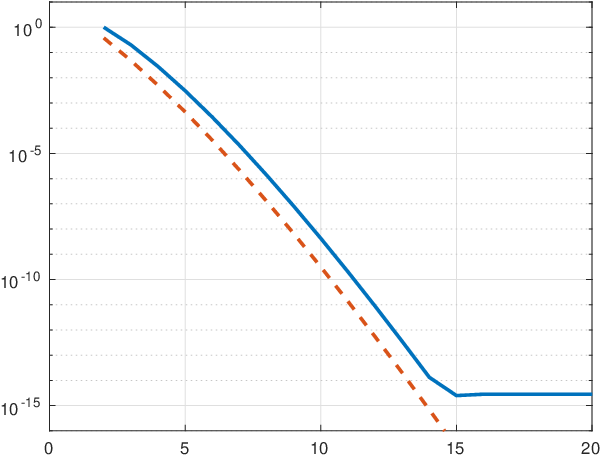
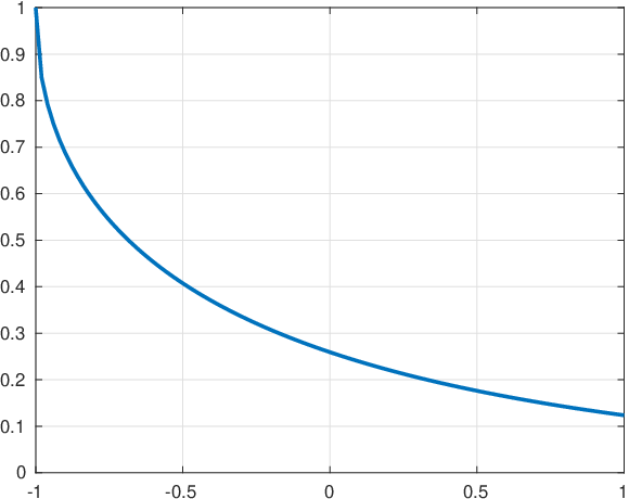
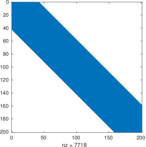
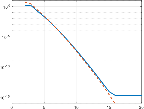
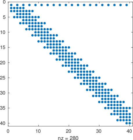
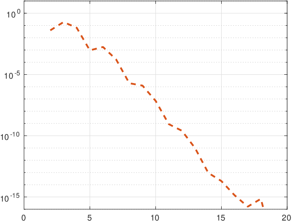
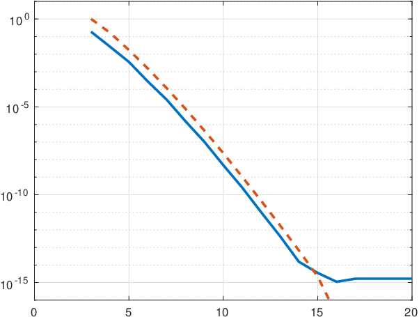
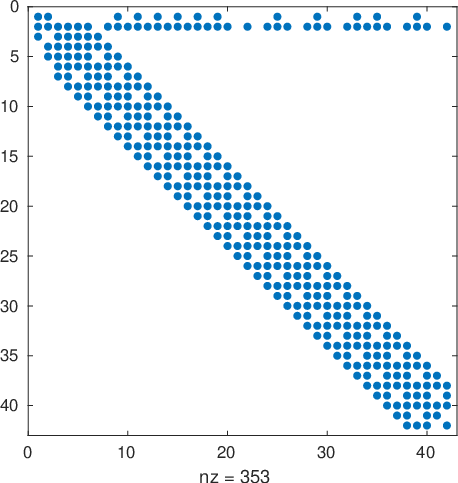
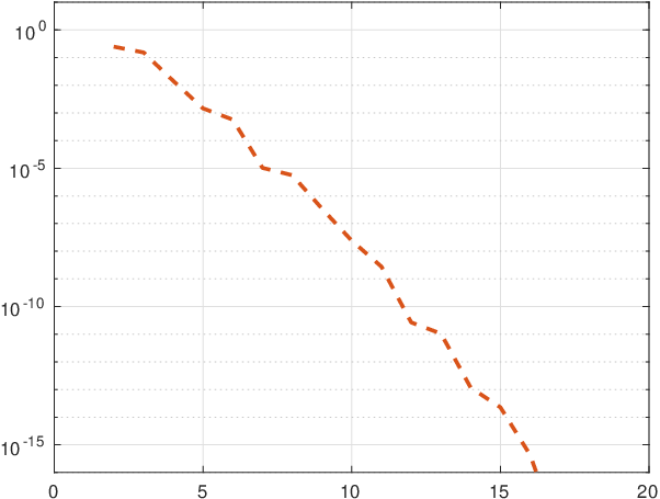
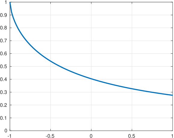
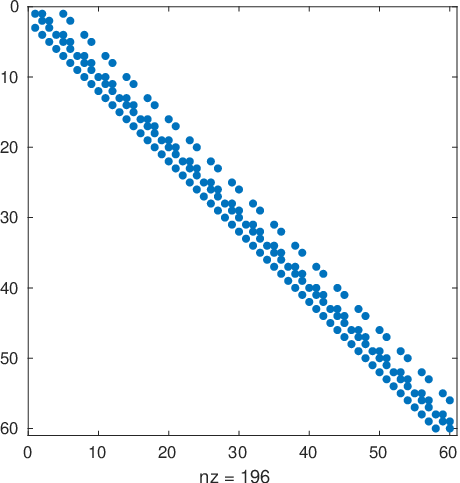
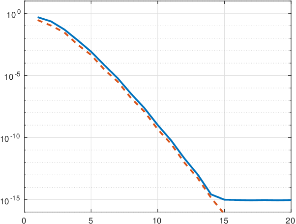
To solve the FDE (67) we form the linear system (66) with σ=1\sigma=1, e¯=(1,0,…)⊤\underline{e}=(1,0,\ldots)^{\top}, and f¯=(0,0,…)⊤\underline{f}=(0,0,\ldots)^{\top}, truncate at some length NN, and solve with \\backslash in MATLAB. The results are shown in Figure 1. The first image shows a plot of the computed solution with N=20N=20. The spy plot in the second image verifies that, upon re-ordering, the associated linear system (66) is tridiagonal. The third image shows two measures of the error in the approximation as NN is increased.99 9 We show both measures here to validate the use of the second, which we employ later when a closed-form expression of the true solution is not readily available. The first (solid line) is computed by evaluating the approximate solution on a 100-point equally-spaced grid in the interval [−1,1][-1,1] using Clenshaw’s algorithm and comparing to the true solution (68). Geometric convergence is observed until it plateaus at around 15 digits of accuracy when NN = 15. The second measure (dashed line) is the 2-norm difference between the coefficients of the approximated solution when truncating at sizes NN and ⌈1.1​N⌉\lceil 1.1N\rceil. Here the convergence does not plateau, suggesting that the computed coefficients maintain good relative accuracy even when their magnitude is below machine precision.
Refer to caption
Refer to caption
Refer to caption

ErrorSpy plot () = N 20 Solutionerror u ( x ) N x

Fig. 1: (a) Approximate solution to (67). (b) MATLAB spy plot showing that truncated linear system (66) is tridiagonal. (c) Two measures of the error in the approximation as NN varies. Solid line: Infinity norm error of solution approximated on a 100-point equally spaced grid. Dashed line: 2-norm difference between the coefficients of the approximated solution when truncating at sizes NN and ⌈1.1​N⌉\lceil 1.1N\rceil. In both cases, geometric convergence is observed.

3.2 Half-order integral equations with non-constant coefficients

In much the same way as in the US method for ODEs [27], the approach outlined above is readily extended to FDEs with non-constant coefficients. In particular, to solve problems of the form

u⁡(x)+r​(x)−1​𝒬x1/2​u​(x)=e⁡(x)+1+x​f​(x),u(x)+r(x)\,_{-1}{\cal{Q}}_{x}^{1/2}u(x)=e(x)+\sqrt{1+x}f(x), (69)

we can appeal to the discussion in Section 2.3 and construct multiplication operators Π𝐏​[r]\Pi_{\mathbf{P}}[r] and Π𝐔​[r]\Pi_{\mathbf{U}}[r], which act on Legendre and second-kind Chebyshev series, respectively. If r⁡(x)r(x) is a polynomial of degree dd, then these two operators will have bandwidth dd. If r⁡(x)r(x) is not a polynomial but is sufficiently smooth (for example, analytic), then the coefficients in its ultraspherical polynomial expansion will decay rapidly, and we may consider Π𝐏​[r]\Pi_{\mathbf{P}}[r] and Π𝐔​[r]\Pi_{\mathbf{U}}[r] as banded for practical purposes. The resulting linear system then takes the form

(I+Π0​[r]​Q1/2)​(a¯b¯)=(e¯f¯),\big(I+\Pi_{0}[r]Q^{1/2}\big)\left(\begin{array}[]{c}\underline{a}\\ \underline{b}\end{array}\right)=\left(\begin{array}[]{c}\underline{e}\\ \underline{f}\end{array}\right), (70)

where Π0​[r]\Pi_{0}[r] is defined in Section 2.6.

We may also consider problems of the form

u⁡(x)+r1​(x)−1​𝒬x1/2​[r2​u]​(x)=e⁡(x)+1+x​f​(x),u(x)+r_{1}(x)_{-1}{\cal{Q}}_{x}^{1/2}\left[r_{2}u\right](x)=e(x)+\sqrt{1+x}f(x), (71)

in which case the linear system becomes

(I+Π0​[r1]​Q1/2​Π0​[r2])​(a¯b¯)=(e¯f¯).\big(I+\Pi_{0}[r_{1}]Q^{1/2}\Pi_{0}[r_{2}]\big)\left(\begin{array}[]{c}\underline{a}\\ \underline{b}\end{array}\right)=\left(\begin{array}[]{c}\underline{e}\\ \underline{f}\end{array}\right). (72)

Similarly, problems of the form

u⁡(x)+(r⁡(x)+1+x​s​(x))−1​𝒬x1/2​u​(x)=e⁡(x)+1+x​f​(x).u(x)+(r(x)+\sqrt{1+x}s(x))\,_{-1}{\cal{Q}}_{x}^{1/2}u(x)=e(x)+\sqrt{1+x}f(x). (73)

and

u(x)+−1𝒬x1/2[(r+1+⋄s)u](x)=e(x)+1+xf(x).u(x)+\,_{-1}{\cal{Q}}_{x}^{1/2}[(r+\sqrt{1+\diamond}s)u](x)=e(x)+\sqrt{1+x}f(x). (74)

may also be solved with linear systems

(I+Π0​[r,s]​Q1/2)​(a¯b¯)=(e¯f¯),\left(I+\Pi_{0}[r,s]Q^{1/2}\right)\left(\begin{array}[]{c}\underline{a}\\ \underline{b}\end{array}\right)=\left(\begin{array}[]{c}\underline{e}\\ \underline{f}\end{array}\right), (75)

and

(I+Q1/2​Π0​[r,s])​(a¯b¯)=(e¯f¯),\left(I+Q^{1/2}\Pi_{0}[r,s]\right)\left(\begin{array}[]{c}\underline{a}\\ \underline{b}\end{array}\right)=\left(\begin{array}[]{c}\underline{e}\\ \underline{f}\end{array}\right), (76)

respectively. However, these systems are no longer banded, and we will lose the linear complexity of our algorithm. Upon reordering they are dense above the diagonal and banded below, so Gaussian elimination will have 𝒪⁡(N2){\cal{O}}(N^{2}) complexity (see Example 3.7 below).

Example 3.6.

We adapt the example of Section 3.5 so that

u(x)+e−1−(1+x)/2𝒬x1/2[e(1+x)/2u](x)=e−(1+x)/2,u(x)+e^{-(1+x)/2}\,_{-1}\mathcal{Q}_{x}^{1/2}[e^{(1+x)/2}u](x)=e^{-(1+x)/2}, (77)

with solution

u⁡(x)=e(1+x)/2​erfc​(1+x).u(x)=e^{(1+x)/2}{\rm{erfc}}(\sqrt{1+x}). (78)

Again taking u⁡(x)u(x) as in (58), the resulting linear system defining the coefficients a¯\underline{a} and b¯\underline{b} is of the form

(I+Π[e−(1+x)/2]Q1/2Π0[e(1+x)/2])(a¯b¯)=(e¯0¯),\left(I+\Pi[e^{-(1+x)/2}]Q^{1/2}\Pi_{0}[e^{(1+x)/2}]\right)\left(\begin{array}[]{c}\underline{a}\\ \underline{b}\end{array}\right)=\left(\begin{array}[]{c}\underline{e}\\ \underline{0}\end{array}\right), (79)

where e¯\underline{e} are the Legendre coefficients of the function e−(1+x)/2e^{-(1+x)/2}. (See Section 6.1 for discussion on how these are computed.) As in the previous example, we truncate each of the expansions at a suitable length NN and solve the resulting finite dimensional banded matrix problem using \\backslash in MATLAB.

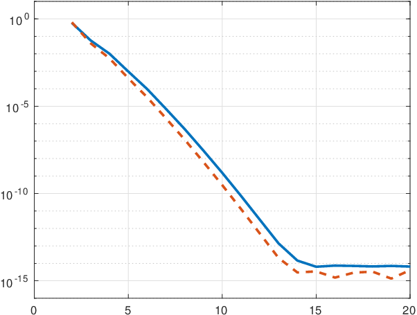
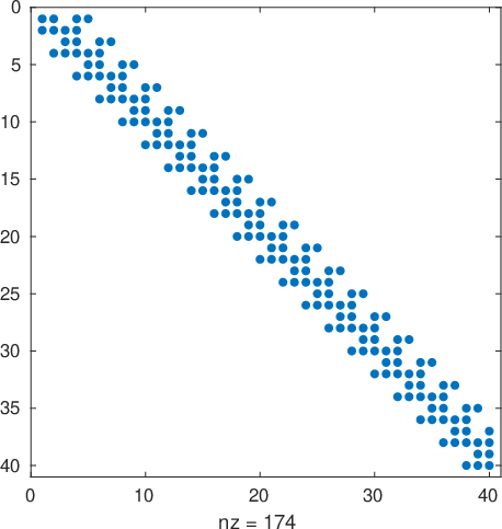
The results are shown in Figure 2. The left panel shows the approximate solution computed with N=20N=20. The centre panel shows a spy plot of the discretised, truncated, and re-ordered operator (79). The non-constant coefficients in equation (77) mean the resulting matrix is no longer tridiagonal, however, it is banded independently of NN and can be solved by \\backslash in linear time as N→∞N\rightarrow\infty. The precise bandwidth depends on the number of Chebyshev coefficients required to approximate the non-constant coefficients, in this case e±(1+x)/2e^{\pm(1+x)/2}, to machine precision accuracy. Here the number of coefficients required is around 14, and the resulting matrix has a bandwidth of approximately 43. The final panel shows the accuracy of the computed solution as NN increases, using the same two forms of the error estimate as described in Example 3.5. Geometric convergence is again observed, but here both measures of the error plateau due to rounding error in the computation of the Chebyshev coefficients of the functions e±(1+x)/2e^{\pm(1+x)/2}.

Refer to caption
Refer to caption
Refer to caption

ErrorSpy plot () = N 100 Solutionerror u ( x ) N x

Fig. 2: (a) Solution to (77). (b) MATLAB spy plot of (79) showing the banded structure. (c) Solid line: Infinity norm error of solution approximated on a 100-point equally spaced grid. Dashed line: 2-norm difference between the coefficients of the approximated solution when truncating at sizes NN and ⌈1.1​N⌉\lceil 1.1N\rceil. Again, geometric convergence is observed.
Example 3.7.

Here we solve

u⁡(x)−erfc​1+x−1​𝒬x1/2​u​(x)=1.u(x)-{\rm erfc}{\sqrt{1+x}}\,_{-1}\mathcal{Q}_{x}^{1/2}u(x)=1. (80)

The linear system satisfied by the coefficients a¯\underline{a} and b¯\underline{b} is then of the form

(I+Π0​[−1,erf⁡(1+x)1+x]​Q1/2)​(a¯b¯)=(10¯).\left(I+\Pi_{0}\!\left[-1,\frac{{\rm erf}(\sqrt{1+x})}{\sqrt{1+x}}\right]Q^{1/2}\right)\left(\begin{array}[]{c}\underline{a}\\ \underline{b}\end{array}\right)=\left(\begin{array}[]{c}1\\ \underline{0}\end{array}\right). (81)

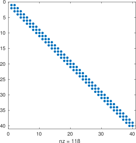
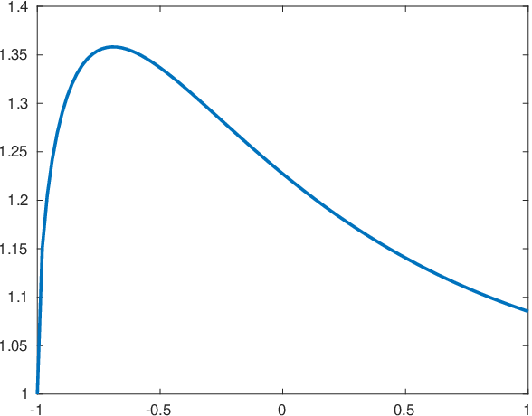
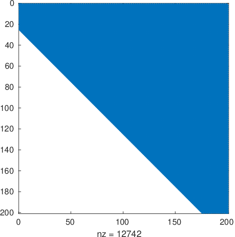
We may truncated and solve (81), and the results of such are shown in Figure 3. Here, in the spy plot in the centre panel we see that, as expected, the required change of bases 𝐏↔𝐔1/2\mathbf{P}\leftrightarrow\mathbf{U}_{1/2} are no longer banded, and hence neither is the re-ordered version of (81). However, the re-ordered matrix is lower-banded, and MATLAB’s \\backslash will require 𝒪⁡(N2){\cal O}(N^{2}) operations to solve such systems directly via Gaussian elimination.

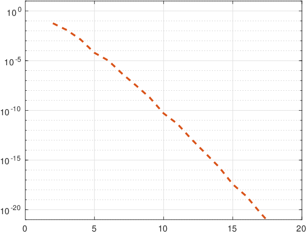
In this case we do not know an explicit form for the solution, and so in the right panel show only the accuracy estimate based upon comparison of successive approximations. We again observe geometric convergence in the number of degrees of freedom until convergence plateaus at around the level of machine precision.
Refer to caption
Refer to caption
Refer to caption

ErrorSpy plot ( = N 100 ) Approximate solution () = N 25 error u ( x ) N x

Fig. 3: (a) Approximate solution to (80). (b) MATLAB spy plot of (81) showing the quasi-upper triangular structure. Such a system will require 𝒪⁡(N2){\cal{O}}(N^{2}) operations to invert. Here a closed-form expression of the solution is not know, so (c) shows the 2-norm difference between the coefficients of the approximated solution when truncating at sizes NN and ⌈1.1​N⌉\lceil 1.1N\rceil. Although the system is no longer banded, geometric convergence is still maintained.

3.3 Higher-Order Integral equations

The approach outlined in the previous few examples extends readily to higher-order integral equations of half-integer order. The general form of the problem we consider is

ℒ​u​(x)=e⁡(x)+1+x​f​(x){\cal{L}}u(x)=e(x)+\sqrt{1+x}f(x) (82)

where

ℒ​u​(x)=α[0]​(x)​u​(x)+∑k=12​mα[k]​(x)−1​𝒬xk/2​[β[k]​u]​(x),\displaystyle{\cal{L}}u(x)=\alpha^{[0]}(x)u(x)+\sum_{k=1}^{2m}\alpha^{[k]}(x)\,_{-1}\mathcal{Q}^{k/2}_{x}[\beta^{[k]}u](x),\hskip 75.0pt (83)
α[k](x)=p[k](x)+1+xq[k](x),β[k](x)=r[k](x)+1+xs[k](x),k=0,1,…,2m,\displaystyle\alpha^{[k]}(x)=p^{[k]}(x)+\sqrt{1+x}q^{[k]}(x),\qquad\beta^{[k]}(x)=r^{[k]}(x)+\sqrt{1+x}s^{[k]}(x),\qquad k=0,1,\ldots,2m, (84)

and all the functions e⁡(x),f⁡(x),p[k]​(x),q[k]​(x),r[k]​(x),s[k]​(x),k=0,1,…,2​me(x),f(x),p^{[k]}(x),q^{[k]}(x),r^{[k]}(x),s^{[k]}(x),\,k=0,1,\ldots,2m are assumed analytic in some neighbourhood of [−1,1][-1,1]. If we continue to take (58) as our ansatz, then we arrive at the infinite dimensional linear system

(Π0​[p[0],q[0]]+∑k=12​mΠ0​[p[k],q[k]]​Qk/2​Π0​[r[k],s[k]])​(a¯b¯)=(e¯f¯),\left(\Pi_{0}[p^{[0]},q^{[0]}]+\sum_{k=1}^{2m}\Pi_{0}[p^{[k]},q^{[k]}]Q^{k/2}\Pi_{0}[r^{[k]},s^{[k]}]\right)\left(\begin{array}[]{c}\underline{a}\\ \underline{b}\end{array}\right)=\left(\begin{array}[]{c}\underline{e}\\ \underline{f}\end{array}\right), (85)

where e¯\underline{e} and f¯\underline{f} are as in (64).

As before, the precise form of this operator will depend on both mm and the number of Chebyshev coefficients required to represent the functions p[k]​(x),q[k]​(x),r[k]​(x),p^{[k]}(x),q^{[k]}(x),r^{[k]}(x), and s[k]​(x)s^{[k]}(x). However, if the q[k]​(x)q^{[k]}(x) and s[k]​(x)s^{[k]}(x) are all identically zero, then (after re-ordering) the operator will remain banded independently of NN. Otherwise it will be lower-bounded, as in Example 3.7.

Example 3.8.

For simplicity, we choose a constant coefficient problem so that the banded structure of the resulting operator is readily observed. In particular, we solve

u(x)−−1𝒬x1/2u(x)+−1𝒬x1u(x)−−1𝒬x3/2u(x)+−1𝒬x2u(x)=1,u(x)-\,_{-1}{\cal{Q}}_{x}^{1/2}u(x)+\,_{-1}{\cal{Q}}_{x}^{1}u(x)-\,_{-1}{\cal{Q}}_{x}^{3/2}u(x)+\,_{-1}{\cal{Q}}_{x}^{2}u(x)=1, (86)

which may be expressed as

(I−Q1/2+Q1−Q3/2+Q2)​(a¯b¯)=(10¯).\left(I-Q^{1/2}+Q^{1}-Q^{3/2}+Q^{2}\right)\left(\begin{array}[]{c}\underline{a}\\ \underline{b}\end{array}\right)=\left(\begin{array}[]{c}1\\ \underline{0}\end{array}\right). (87)

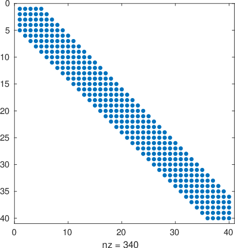
As in the previous examples, we truncate this operator at a given size NN and solve the resulting finite dimensional problem. The results are shown in Figure 4 with the first and second panels showing the approximated solution and spy plot of (87) when N=20N=20, respectively. The third panel shows the convergence of the solution. As in the Example 3.7 we do not know the true solution, so we estimate the error by the 2-norm difference between the coefficients of the approximated solution when truncating at sizes NN and ⌈1.1​N⌉\lceil 1.1N\rceil. We again observe geometric convergence, and as in Example 3.5, the error continues to decrease even below the level of machine precision for this constant coefficient problem.
Refer to caption
Refer to caption
Refer to caption

ErrorSpy plot ( = N 20 ) Approximate solution ( = N 20 ) error u ( x ) N x

Fig. 4: (a) Approximate solution to (86). (b) MATLAB spy plot of (87) showing the banded structure of the linear system. (c) 2-norm difference between the coefficients of the approximated solution when truncating at sizes NN and ⌈1.1​N⌉\lceil 1.1N\rceil. Even for higher-order problems, geometric convergence is obtained. As in Example 1, since there are no-constant coefficients whose Chebyshev coefficients must be computed, this measure of the error continues to converge below machine precision.

4 FDEs: Riemann–Liouville definition

Our approach here for FDEs of Riemann–Liouville-type will be similar to the FIEs above. The main difference will stem from the fact that the operators DmD^{m} and Dm+1/2D^{m+1/2} defined in Section 2.6 no longer map to the same direct sum spaces and we must make use of the block-banded conversion operators EmE_{m} and Em+1/2E_{m+1/2} (analogous to how the conversion operators 𝒮λ{\cal S}_{\lambda} are used in [27]).

4.1 Differential equation of order 1/21/2

Consider the FDE

u⁡(x)+Dx1/2−1R​L​u​(x)=e⁡(x)+11+x​f​(x),x∈[−1,1],u⁡(−1)<∞,u(x)+\prescript{RL}{-1}{D^{1/2}_{x}}u(x)=e(x)+\frac{1}{\sqrt{1+x}}f(x),\qquad x\in[-1,1],\qquad u(-1)<\infty, (88)

(sometimes called a “fractional relaxation equation”) and make the same ansatz as before that

u⁡(x)\displaystyle u(x) =\displaystyle= ∑n=0∞an​Pn​(x)+1+x​∑n=0∞bn​Un​(x)=[𝐏⁡(x),𝐔1/2​(x)]​(a¯b¯).\displaystyle\sum_{n=0}^{\infty}a_{n}P_{n}(x)+{\sqrt{1+x}}\sum_{n=0}^{\infty}b_{n}U_{n}(x)=\left[\mathbf{P}(x),\mathbf{U}_{1/2}(x)\right]\left(\begin{array}[]{c}\underline{a}\\ \underline{b}\end{array}\right).

From Section 2.6 we have that

𝒟x1/2−1R​L​u​(x){}^{RL}_{-1}\mathcal{D}^{1/2}_{x}u(x) =\displaystyle= [𝐂(3/2)(x),𝐔−1/2(x)]D1/2(a¯b¯),\displaystyle\left[\mathbf{C}^{(3/2)}(x),\mathbf{U}_{-1/2}(x)\right]D^{1/2}\left(\begin{array}[]{c}\underline{a}\\ \underline{b}\end{array}\right),

where D1/2D^{1/2} is defined in (48). As mentioned above, and unlike in the case of the integral equations, the range of 𝒟x1/2−1R​L​u​(x)\prescript{RL}{-1}{{\cal{D}}}^{1/2}_{x}u(x) is not the same as that of u⁡(x)u(x). However, we can find a banded transform from 𝐏⊕𝐔1/2\mathbf{P}\oplus\mathbf{U}_{1/2} to 𝐂(3/2)(x)⊕𝐔−1/2\mathbf{C}^{(3/2)}(x)\oplus\mathbf{U}_{-1/2} using E1/2E_{1/2} so that

u⁡(x)\displaystyle u(x) =\displaystyle= [𝐂(3/2)(x),𝐔−1/2(x)]E1/2(a¯b¯).\displaystyle\left[\mathbf{C}^{(3/2)}(x),\mathbf{U}_{-1/2}(x)\right]E_{1/2}\left(\begin{array}[]{c}\underline{a}\\ \underline{b}\end{array}\right).

This time letting

e(x)+11+xf(x)=[𝐂(3/2)(x),𝐔−1/2(x)](e¯f¯)e(x)+\frac{1}{\sqrt{1+x}}f(x)=\left[\mathbf{C}^{(3/2)}(x),\mathbf{U}_{-1/2}(x)\right]\left(\begin{array}[]{c}\underline{e}\\ \underline{f}\end{array}\right) (98)

and equating coefficients leads to the linear system of equations

(E1/2+D1/2)​(a¯b¯)=(S𝐏D𝐔1/21/2D𝐏1/2R𝐔)​(a¯b¯)=(e¯f¯).\left(\begin{array}[]{c c}E_{1/2}+D^{1/2}\end{array}\right)\left(\begin{array}[]{c}\underline{a}\\ \underline{b}\end{array}\right)=\left(\begin{array}[]{c c}S_{\mathbf{P}}&D_{\mathbf{U}_{1/2}}^{1/2}\\ D_{\mathbf{P}}^{1/2}&R_{\mathbf{U}}\end{array}\right)\left(\begin{array}[]{c}\underline{a}\\ \underline{b}\end{array}\right)=\left(\begin{array}[]{c}\underline{e}\\ \underline{f}\end{array}\right). (99)

Again, each block of the operators in (99) are banded, and by interleaving the coefficients so that (a¯⊤,b¯⊤)(\underline{a}^{\top},\underline{b}^{\top}) ↦\mapsto (a0,b0,a1,b1,…)⊤(a_{0},b_{0},a_{1},b_{1},\ldots)^{\top} we can convert the above to a banded system.

Remark: One can show that the null space of the operator on the left-hand side of (88) acting on functions in L1L_{1} is

v⁡(x)=E1/2,1/2​(−1+x)1+x,v(x)=\frac{E_{1/2,1/2}(-\sqrt{1+x})}{\sqrt{1+x}}, (100)

(where E1/2,1/2E_{1/2,1/2} is the Mittag-Leffler function [12, 10.46.3]) [6, p. 13], which is unbounded at x=−1x=-1. Since our trial space (4.1) contains only bounded functions on [−1,1][-1,1], we need not enforce a boundary condition explicitly in this case. We discuss boundary constraints in more detail momentarily. To allow solutions which are unbounded at the left end of the domain then one possibility is to use instead the ansatz u(x)=𝐏(x)a¯+𝐓−1/2(x)b¯u(x)=\mathbf{P}(x)\underline{a}+\mathbf{T}_{-1/2}(x)\underline{b}, where 𝐓⁡(x)\mathbf{T}(x) is the quasimatrix whose columns are formed of Chebyshev polynomials of the first kind, Tn​(x),n=0,1,…T_{n}(x),\,n=0,1,\ldots. One can derive similar banded operators to all those introduced in Section 2, but we omit the details (which are complicated by the fact that Tn​(x)T_{n}(x) is not an ultraspherical polynomial and therefore many of the formulae in Section 2 differ subtly).

Example 4.9.

We consider a modification of the second-kind Abel integral equation in Example 3.5, namely

u(x)+−1𝒟x1/2u(x)=1π​1+x,u(−1)<∞,u(x)+_{-1}\mathcal{D}_{x}^{1/2}u(x)=\frac{1}{\sqrt{\pi}\sqrt{1+x}},\qquad u(-1)<\infty, (101)

with solution

u⁡(x)=e1+x​erfc​(1+x).u(x)=e^{1+x}\rm{erfc}(\sqrt{1+x}). (102)

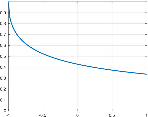
To solve we choose an NN and form the system (99) with e¯=0¯\underline{e}=\underline{0} and f¯=[1/π,0,0,…]⊤\underline{f}=[1/\sqrt{\pi},0,0,\ldots]^{\top}. Results are shown in Figure 5. As usual, the first two panels show a plot of the solution and a spy plot of the discretised operator when N=20N=20. The spy plot verifies that the matrix is banded (here with bandwidth four) and hence that the system (99) can be solved in linear time with MATLAB’s \\backslash. The final panel shows both the infinity norm error (approximated on a 100-point equally spaced grid) of computed solution compared to the exact solution (102) (solid line) and the 2-norm difference between the coefficients of the approximated solution when truncating at sizes NN and ⌈1.1​N⌉\lceil 1.1N\rceil (dashed line). Again we observe geometric convergence.
Refer to caption
Refer to caption
Refer to caption

ErrorSpy plot ( = N 20 ) Solutionerror u ( x ) N x

Fig. 5: (a) Solution to (101). (b) MATLAB spy plot of (99) showing the banded structure (c) Solid line: Infinity norm error of solution approximated on a 100-point equally spaced grid. Dashed line: 2-norm difference between the coefficients of the approximated solution when truncating at sizes NN and ⌈1.1​N⌉\lceil 1.1N\rceil. As in the case of FIEs from the previous section, geometric convergence is observed here for this FDE.

4.2 Differential equation of order 11 and 1/21/2

Here we consider

u⁡(x)+Dx1/2−1R​L​u​(x)+u′​(x)=e⁡(x)+11+x​f​(x),x∈[−1,1],u(x)+\prescript{RL}{-1}{D^{1/2}_{x}}u(x)+u^{\prime}(x)=e(x)+\frac{1}{\sqrt{1+x}}f(x),\qquad x\in[-1,1], (103)

along with a suitable initial or boundary condition, or some other functional constraint (see below). Now

u′​(x)\displaystyle u^{\prime}(x) =\displaystyle= [𝐂(3/2)(x),𝐂−1/2(2)(x)]D(a¯b¯),\displaystyle\left[\mathbf{C}^{(3/2)}(x),\mathbf{C}^{(2)}_{-1/2}(x)\right]D\left(\begin{array}[]{c}\underline{a}\\ \underline{b}\end{array}\right),

where DD is defined in (48). We must modify the spaces of both u¯\underline{u} and D1/2​u¯D^{1/2}\underline{u} accordingly, and so arrive at

(E1​E1/2+E1​D1/2+D)​(a¯b¯)=(e¯f¯),\left(E_{1}E_{1/2}+E_{1}D^{1/2}+D\right)\left(\begin{array}[]{c}\underline{a}^{\vphantom{(k)}}_{\vphantom{(k)}}\\ \underline{b}\end{array}\right)=\left(\begin{array}[]{c}\underline{e}^{\vphantom{(k)}}_{\vphantom{(k)}}\\ \underline{f}\end{array}\right), (107)

where

e⁡(x)=∑n=0∞en​Cn(3/2)​(x),f⁡(x)=∑n=0∞fn​Cn(2)​(x).e(x)=\sum_{n=0}^{\infty}e_{n}C_{n}^{(3/2)}(x),\qquad f(x)=\sum_{n=0}^{\infty}f_{n}C_{n}^{(2)}(x). (108)

Again, by interleaving the coefficients, we can make the above operator banded.

4.2.1 Boundary conditions

In this case, the kernel of the operator in (103) is smooth and we must enforce a boundary condition to ensure that the linear system (107) is invertible. The topic of boundary conditions in FDEs is complicated, and it is beyond the scope of this paper to give a full treatment here. Here we simply show how certain boundary conditions/side constraints can be applied to linear systems such as (107) and leave it to the reader to determine how many and what form of constraints are applicable to their FDE.

For example, consider the functional constraint ℬx​u:=u⁡(x)=c.{\cal B}^{x}u:=u(x)=c. Given scalar x∈[−1,1]x\in[-1,1] we can construct this functional acting on a basis in 𝐂γ(λ)\mathbf{C}^{(\lambda)}_{\gamma} as a row vector by defining Bλ,γx:𝐂γ(λ)→ℂB_{\lambda,\gamma}^{x}:\mathbf{C}^{(\lambda)}_{\gamma}\rightarrow\mathbb{C} as Bλ,γx:=𝐂γ(λ)​(x)B_{\lambda,\gamma}^{x}:=\mathbf{C}^{(\lambda)}_{\gamma}(x). In particular, x=−1x=-1 corresponds to a boundary/initial condition on the left and x=+1x=+1 to a boundary condition on the right. Some useful cases are

B𝐏−1=[1,−1,1,−1,…],B𝐔1/2−1=[0,0,…],B𝐏+1=[1,1,…],andB𝐔1/2+1=2[1,2,3,4,…].B_{\mathbf{P}}^{-1}=[1,-1,1,-1,\ldots],\quad B_{\mathbf{U}_{1/2}}^{-1}=[0,0,\ldots],\quad B_{\mathbf{P}}^{+1}=[1,1,\ldots],\quad\text{and}\quad B_{\mathbf{U}_{1/2}}^{+1}=\sqrt{2}[1,2,3,4,\ldots]. (109)

Combining such operators to act on our direct sum expansion of the solution u⁡(x)u(x), we have, for example, B−1:𝐏⊕𝐔1/2→ℂB^{-1}:\mathbf{P}\oplus\mathbf{U}_{1/2}\rightarrow\mathbb{C} given by B−1=[B𝐏−1,B𝐔1/2−1]B^{-1}=[B_{\mathbf{P}}^{-1},B_{\mathbf{U}_{1/2}}^{-1}] and our system (107) augmented with the boundary condition u⁡(−1)=cu(-1)=c becomes

(B−1E1​E1/2+E1​D1/2+D)⁡(a¯b¯)=(c[e¯f¯]),\begin{pmatrix}B^{-1}\cr E_{1}E_{1/2}+E_{1}D^{1/2}+D\end{pmatrix}\left(\begin{array}[]{c}\underline{a}\\ \underline{b}\end{array}\right)=\left(\begin{array}[]{c}c\\ \left[\begin{array}[]{c}\underline{e}^{\vphantom{(k)}}_{\vphantom{(k)}}\\ \underline{f}\end{array}\right]\end{array}\right), (110)

Upon the usual re-ordering of the coefficients, this becomes an almost-banded infinite matrix—that is, banded apart from a finite number of dense rows—and when truncated to a (2​N+1)×(2​N+1)(2N+1)\times(2N+1) finite matrix is solvable in O⁡(N)O(N) operations using either a Schur complement factorisation about the (1,1)(1,1) entry, the Woodbury matrix identity, or by using the adaptive QR method described in [27]. See Section 6.2 for more details.

Example 4.10.

Consider the case of (103) where the right-hand side is zero and u⁡(−1)=1u(-1)=1:

u⁡(x)+Dx1/2−1R​L​u​(x)+u′​(x)=0,x∈[−1,1],u(x)+\prescript{RL}{-1}{D^{1/2}_{x}}u(x)+u^{\prime}(x)=0,\qquad x\in[-1,1], (111)

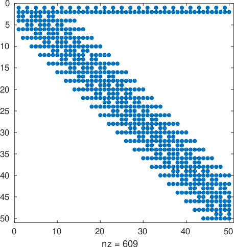
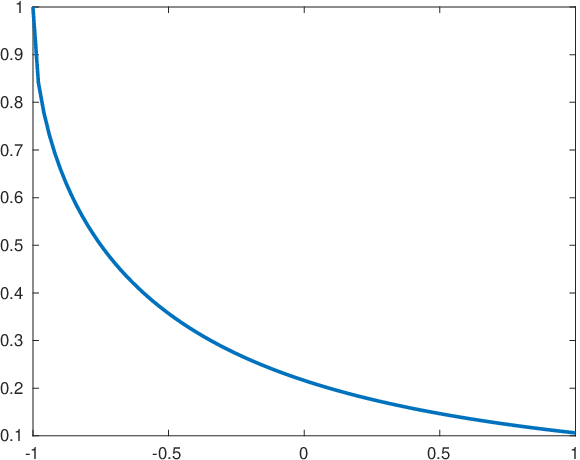
which amounts to taking c=1c=1 and e¯=f¯=0¯\underline{e}=\underline{f}=\underline{0} in (110). The computed solution is depicted in the left panel of Figure 6. The middle panel verifies the almost banded nature of the operator (110), and the right panel demonstrates geometric convergence.
Refer to caption
Refer to caption
Refer to caption

ErrorSpy plot ( = N 20 ) Approximate solution () = N 20 error u ( x ) N x

Fig. 6: (a) Approximate solution to (111). (b) MATLAB spy plot of (110) showing the almost-banded structure. (c) 2-norm difference between the coefficients of the approximated solution when truncating at sizes NN and ⌈1.1​N⌉\lceil 1.1N\rceil showing geometric convergence.

4.3 Non-constant coefficients

Non-constant coefficients can be dealt with in a similar way as described for fractional integral equations in Section 3.2. We omit the details.

4.4 Higher order

Similarly to the case of integral equations, the approach outlined above can be extended to higher-order derivatives. Consider the general mmth half-integer order FDE:

ℒ​u​(x)=α[0]​(x)​u​(x)+∑k=12​mα[k]​(x)−1​𝒟xk/2​[β[k]​u]​(x),{\cal{L}}u(x)=\alpha^{[0]}(x)u(x)+\sum_{k=1}^{2m}\alpha^{[k]}(x)\,_{-1}\mathcal{D}^{k/2}_{x}[\beta^{[k]}u](x), (112)

where the nonconstant coefficients α[k]​(x)\alpha^{[k]}(x) and β[k]​(x)\beta^{[k]}(x) are analytic in some neighbourhood of [−1,1][-1,1]. If we continue to take as our anzatz solution the function

u⁡(x)=[𝐏⁡(x),𝐔1/2​(x)]​(a¯b¯)u(x)=\left[\mathbf{P}(x),\mathbf{U}_{1/2}(x)\right]\left(\begin{array}[]{c}\underline{a}\\ \underline{b}\end{array}\right) (113)

then we have L:𝐏⊕𝐔1/2→𝐂(m+1/2)⊕𝐂−m+1/2(m+1)L:\mathbf{P}\oplus\mathbf{U}_{1/2}\rightarrow\mathbf{C}^{(m+1/2)}\oplus\mathbf{C}^{(m+1)}_{-m+1/2} given by

(∑k=02​m−1(Em​Em−1/2​…​E(k+1)/2)​Πk/2​[α[k]]​Dk/2​Π​[β[k]])+Πm​[α[2​m]]​Dm​Π​[β[2​m]]\left(\sum_{k=0}^{2m-1}\left(E_{m}E_{m-1/2}\ldots E_{(k+1)/2}\right)\Pi_{k/2}[\alpha^{[k]}]D^{k/2}\Pi[\beta^{[k]}]\right)+\Pi_{m}[\alpha^{[2m]}]D^{m}\Pi[\beta^{[2m]}] (114)

(where we have defined β[0]​(x)=1\beta^{[0]}(x)=1 for the sake of brevity).

Example 4.11.

Consider the classical Bagley–Torvik equation[4, 5]

u′′​(x)+Dx1/2−1R​L​u​(x)+u⁡(x)=0,\displaystyle u^{\prime\prime}(x)+\prescript{RL}{-1}{D^{1/2}_{x}}u(x)+u(x)=0, x∈[−1,1]\displaystyle\qquad x\in[-1,1] (115)

but here treated as a boundary value problem with

u⁡(−1)=1,andu⁡(1)=0.\displaystyle u(-1)=1,\quad\text{and}\quad u(1)=0. (116)

Following the approach outlined above, we arrive at the infinite dimensional linear system

(B−1B+1D2+E2​E3/2​E1​(D1/2+E1/2))⁡(a¯b¯)=(01[e¯f¯]),\begin{pmatrix}B^{-1}\\ B^{+1}\\ D^{2}+E_{2}E_{3/2}E_{1}(D^{1/2}+E_{1/2})\end{pmatrix}\left(\begin{array}[]{c}\underline{a}^{\vphantom{(k)}}_{\vphantom{(k)}}\\ \underline{b}\end{array}\right)=\left(\begin{array}[]{c}0\\ 1\\ \left[\begin{array}[]{c}\underline{e}^{\vphantom{(k)}}_{\vphantom{(k)}}\\ \underline{f}\end{array}\right]\end{array}\right), (117)

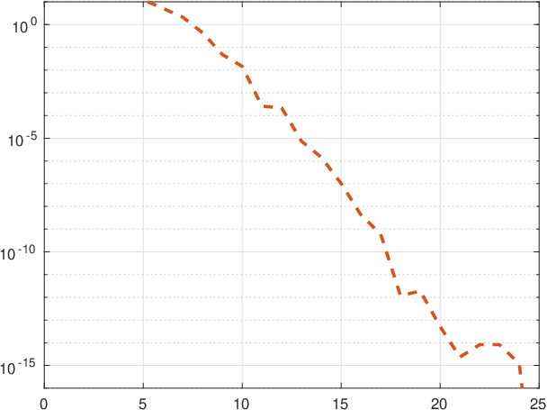
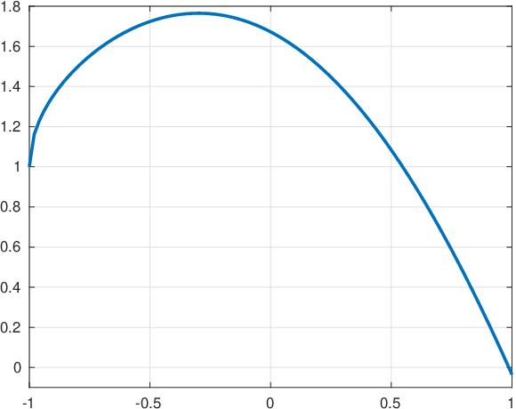
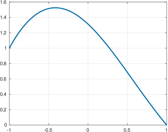
which can be solved in the same manner as before. The solution is depicted in Figure 7.
Refer to caption
Refer to caption
Refer to caption

ErrorSpy plot () = N 25 Approximate solution () = N 25 error u ( x ) N x

Fig. 7: (a) Approximate solution to the Bagley–Torvik equation (115). (b) MATLAB spy plot of (117) demonstrating the almost-banded structure of the linear system. (c) 2-norm difference between the coefficients of the approximated solution when truncating at sizes NN and ⌈1.1​N⌉\lceil 1.1N\rceil showing geometric convergence.

Remark: If we instead consider the FDE: u′′​(x)+D−1R​L​ux3/2​(x)+u⁡(x)=0u^{\prime\prime}(x)+\prescript{RL}{-1}{D}{}^{3/2}_{x}u(x)+u(x)=0, then we simply change the final block-row of the system (117) to D2+E2​(D3/2+E3/2​E1​E1/2)D^{2}+E_{2}(D^{3/2}+E_{3/2}E_{1}E_{1/2}). Similarly, we could incorporate a Neumann or fractional Neumann boundary condition at, say, the right boundary by changing the B+1B^{+1} row to the appropriate functional row.

5 FDEs: Caputo definition

FDEs with the Caputo definition of the fractional derivative can be readily solved by combining our approach for FIEs described in Section 3 with an integral reformulation of the problem. In particular, setting v​(x)=u(⌈m⌉)​(x)v(x)=u^{(\lceil m\rceil)}(x) and therefore u⁡(x)=Q⌈m⌉​v​(x)+p⁡(x)u(x)=Q^{\lceil m\rceil}v(x)+p(x), p⁡(x)∈ℙ⌈m⌉−1p(x)\in\mathbb{P}^{\lceil m\rceil-1}, it follows from the definition of the Caputo derivative that an mmth-order FDE in u⁡(x)u(x) becomes an mmth-order FIE in v⁡(x)v(x) with ⌈m⌉\lceil m\rceil additional boundary constraints to determine the coefficients of the polynomial p⁡(x)=c0+c1​P1​(x)+…​c⌈m⌉−1​P⌈m⌉−1​(x)p(x)=c_{0}+c_{1}P_{1}(x)+\ldots c_{\lceil m\rceil-1}P^{\lceil m\rceil-1}(x). We proceed by example.

Example 5.12.

Consider the Caputo fractional relaxation equation

u⁡(x)+𝒟x1/2−1C​u​(x)=0,u⁡(−1)=1,u(x)+\prescript{C}{-1}{\mathcal{D}}_{x}^{1/2}u(x)=0,\qquad u(-1)=1, (118)

which has the solution

u⁡(x)=e1+x​erfc​(1+x).u(x)=e^{1+x}\text{erfc}(\sqrt{1+x}). (119)

Letting v=u′v=u^{\prime} we have u=𝒬​v+c0u=\mathcal{Q}v+c_{0} and (118) becomes

𝒬v(x)+−𝒬x1/2v(x)+c0\displaystyle\mathcal{Q}v(x)+_{-1\!\!}\mathcal{Q}_{x}^{1/2}v(x)+c_{0} =\displaystyle= 0,\displaystyle 0, (120)
𝒬​v​(−1)+c0\displaystyle\mathcal{Q}v(-1)+c_{0} =\displaystyle= 1.\displaystyle 1. (121)

In operator form, we may write this as the infinite dimensional system

(1B−1​Q[e¯10¯]Q+Q1/2)​(c0[a¯^b¯^])=(10¯),\left(\begin{array}[]{c c}1&B^{-1}Q\\ \left[\begin{array}[]{c}\underline{e}_{1}\\ \underline{0}\end{array}\right]&Q+Q^{1/2}\end{array}\right)\left(\begin{array}[]{c}c_{0}\\ \left[\begin{array}[]{c}\underline{\hat{a}}\\ \underline{\hat{b}}\end{array}\right]\end{array}\right)=\left(\begin{array}[]{c}1\\ \underline{0}\end{array}\right), (122)

where

v⁡(x)=∑n=0∞a^n​Pn​(x)+1+x​b^n​Un​(x)=[𝐏⁡(x),𝐔1/2​(x)]​(a¯^b¯^)v(x)=\sum_{n=0}^{\infty}\hat{a}_{n}P_{n}(x)+\sqrt{1+x}\hat{b}_{n}U_{n}(x)=[\mathbf{P}(x),\mathbf{U}_{1/2}(x)]\left(\begin{array}[]{c}\underline{\hat{a}}\\ \underline{\hat{b}}\end{array}\right) (123)

and B−1=[B𝐏−1,B𝐔1/2−1]B^{-1}=[B_{\mathbf{P}}^{-1},B^{-1}_{\mathbf{U}_{1/2}}]. After truncating and solving this system for the approximate coefficients of v⁡(x)v(x), we can recover those of u⁡(x)u(x) via

(a¯b¯)=Q​(a¯^b¯^)+(c00¯),\left(\begin{array}[]{c}\underline{a}\\ \underline{b}\end{array}\right)=Q\left(\begin{array}[]{c}\underline{\hat{a}}\\ \underline{\hat{b}}\end{array}\right)+\left(\begin{array}[]{c}c_{0}\\ \underline{0}\end{array}\right), (124)

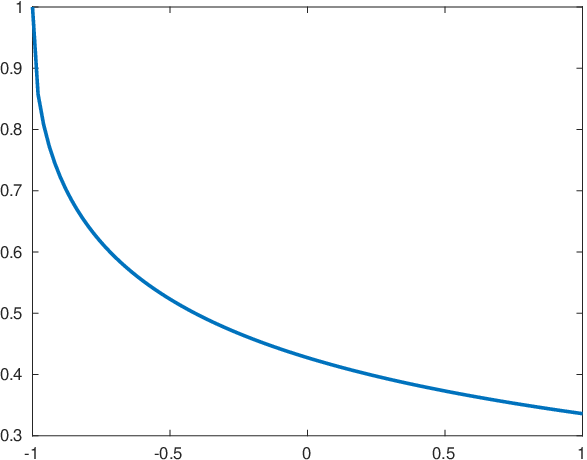
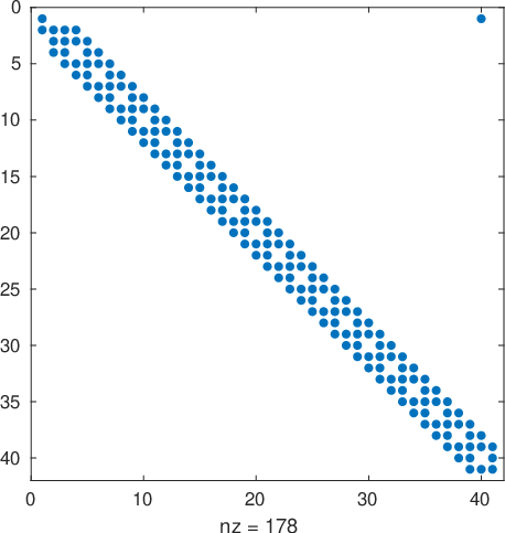
so that, as usual, u⁡(x)=[𝐏⁡(x),𝐔1/2​(x)]​[a¯⊤,b¯⊤]⊤u(x)=[\mathbf{P}(x),\mathbf{U}_{1/2}(x)][\underline{a}^{\top},\underline{b}^{\top}]^{\top}. Figure 8 shows the results. As in the case of RL FDEs we see that the resulting discretised system is almost banded and that the approximation converges geometrically in the number of degrees of freedom.
Refer to caption
Refer to caption
Refer to caption

ErrorSpy plot () = N 20 Solutionerror u ( x ) N x

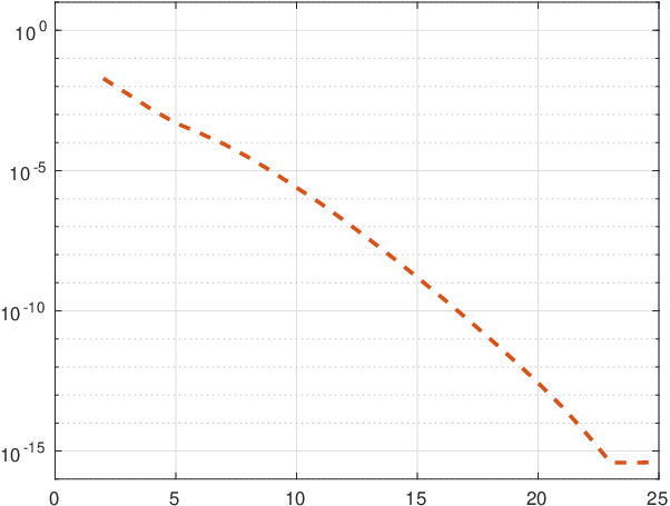
Fig. 8: (a) Solution to the FDE (118). (b) MATLAB spy plot of (122) showing the almost-banded structure. (c) Solid line: Infinity norm error of solution approximated on a 100-point equally spaced grid. Dashed line: 2-norm difference between the coefficients of the approximated solution when truncating at sizes NN and ⌈1.1​N⌉\lceil 1.1N\rceil. As in the case of FIEs and RL-type FDEs of previous two sections, geometric convergence is observed.
Example 5.13.

Consider the Bagley–Torvik equation from Example 4.11, but now using the Caputo definition of the half-derivative:

u′′​(x)+Dx1/2−1C​u​(x)+u⁡(x)=0,\displaystyle u^{\prime\prime}(x)+\prescript{C}{-1}{D}^{1/2}_{x}u(x)+u(x)=0, x∈[−1,1],\displaystyle\qquad x\in[-1,1], (125)
u⁡(−1)=1,\displaystyle u(-1)=1, u⁡(1)=0.\displaystyle\qquad u(1)=0. (126)

This time letting v=u′′v=u^{\prime\prime} we have u=𝒬2​v+c0​P0​(x)+c1​P1​(x)u=\mathcal{Q}^{2}v+c_{0}P_{0}(x)+c_{1}P_{1}(x) and

v(x)+−𝒬x3/2v(x)+c1𝒬x1/2P1′(x)+𝒬2v(x)+c0P0(x)+c1P1(x)\displaystyle v(x)+_{-1\!\!}\mathcal{Q}_{x}^{3/2}v(x)+c_{1}\mathcal{Q}_{x}^{1/2}P_{1}^{\prime}(x)+\mathcal{Q}^{2}v(x)+c_{0}P_{0}(x)+c_{1}P_{1}(x) =\displaystyle= 0,\displaystyle 0, (127)
𝒬2​v​(−1)+c0+c1​P1​(−1)\displaystyle\mathcal{Q}^{2}v(-1)+c_{0}+c_{1}P_{1}(-1) =\displaystyle= 1,\displaystyle 1, (128)
𝒬2​v​(1)+c0+c1​P1​(1)\displaystyle\mathcal{Q}^{2}v(1)+c_{0}+c_{1}P_{1}(1) =\displaystyle= 0.\displaystyle 0. (129)

We may write this as

(1−1B−1​Q211B+1​Q2[e¯10¯]Q1/2​[S1/2−1​D1/2​e¯10¯]+[e¯10¯]Q2+Q3/2+I)​(c0c1[a¯^b¯^])=(10[0¯0¯]),\left(\begin{array}[]{c c c}1&-1&B^{-1}Q^{2}\\ 1&1&B^{+1}Q^{2}\\ \left[\begin{array}[]{c}{\underline{e}_{1}}\\ {\underline{0}}\end{array}\right]&Q^{1/2}\left[\begin{array}[]{c}S^{-1}_{1/2}D_{1/2}\underline{e}_{1}\\ \underline{0}\end{array}\right]+\left[\begin{array}[]{c}{\underline{e}_{1}}\\ {\underline{0}}\end{array}\right]&Q^{2}+Q^{3/2}+I\\ \end{array}\right)\left(\begin{array}[]{c}c_{0}\\ c_{1}\\ \left[\begin{array}[]{c}\underline{\hat{a}}\\ \underline{\hat{b}}\end{array}\right]\end{array}\right)=\left(\begin{array}[]{c}1\\ 0\\ \left[\begin{array}[]{c}\underline{0}\\ \underline{0\vphantom{\hat{b}}}\end{array}\right]\end{array}\right), (130)

where v⁡(x)=∑n=0∞a^n​Pn​(x)+1+x​b^n​Un​(x)v(x)=\sum_{n=0}^{\infty}\hat{a}_{n}P_{n}(x)+\sqrt{1+x}\hat{b}_{n}U_{n}(x) and we have used the fact that P1​(±1)=±1P_{1}(\pm 1)=\pm 1. Once we have solved this system for the approximate coefficients of vv, we can recover those of uu via

(a¯b¯)=Q​(a¯^b¯^)+(c0c10¯),\left(\begin{array}[]{c}\underline{a}\\ \underline{b}\end{array}\right)=Q\left(\begin{array}[]{c}\underline{\hat{a}}\\ \underline{\hat{b}}\end{array}\right)+\left(\begin{array}[]{c}c_{0}\\ c_{1}\\ \underline{0}\end{array}\right), (131)

where here 0¯\underline{0} is a vector of zeros of length 2​N−22N-2. Figure 9 shows the results. Compare with Riemann–Liouville version in Example 4.11.
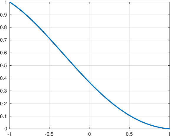
Refer to caption
Refer to caption
Refer to caption

ErrorSpy plot () = N 20 Approximate solution () = N 20 x error u ( x ) N x

Fig. 9: (a) Approximate solution to the Bagley–Torvik equation (125). (b) MATLAB spy plot of (130) showing the almost-banded structure. (c) 2-norm difference between the coefficients of the approximated solution when truncating at sizes NN and ⌈1.1​N⌉\lceil 1.1N\rceil. Compare with the solution on the RL Bagley–Torvik equation in Figure 7.

6 Computational issues

In this section we outline some practical considerations required to perform computations.

6.1 Representing the right-hand side

An essential part of this approach is representing the right-hand side in the direct sum basis 𝐏⊕𝐔1/2\mathbf{P}\oplus\mathbf{U}_{1/2} and its higher-order cousins involving higher order ultraspherical polynomials. A substantial issue is that given a general right-hand side g⁡(x)g(x) the decomposition as, for example,

g⁡(x)=∑n=0∞en​Pn​(x)+1+x​∑n=0∞fn​Un​(x),g(x)=\sum_{n=0}^{\infty}e_{n}P_{n}(x)+\sqrt{1+x}\sum_{n=0}^{\infty}f_{n}U_{n}(x), (132)

is not unique: 𝐏⁡(x)\mathbf{P}(x) and 𝐔1/2​(x)\mathbf{U}_{1/2}(x) form a frame [8]. In the context of this numerical approach, uniqueness is not critical as any expansion of this form is suitable provided we can approximate g⁡(x)g(x) well by taking finite number of terms.

We will assume we are given e⁡(x)e(x) and f⁡(x)f(x) that can be evaluated pointwise1010 10 The case where we may only sample OPENg​x)gx) is beyond the scope of this paper, though solving a least squares system with more points than coefficients can perform well in practice. Another situation that arises in practical settings is where g⁡(x)g(x) is specified by a formula such as exp⁡(x)​1+x+cos⁡x+exp⁡((1+x)/2)​erfc​(1+x)\exp(x)\sqrt{1+x}+\cos x+\exp((1+x)/2)\,{\rm erfc}(\sqrt{1+x}). The approach taken by ApproxFun is to overload each operation to automatically determine an appropriate decomposition. so that

g⁡(x)=e⁡(x)+1+x​f​(x).g(x)=e(x)+\sqrt{1+x}f(x). (133)

In this case, we can calculate the number of Chebyshev coefficients of ee and/or ff to within a required tolerance using an adaptive algorithm [3, 13]. The algorithm is based on the discrete cosine transform (DCT) and hence takes 𝒪⁡(d​log⁡d){\cal{O}}(d\log d) operations to compute dd coefficients. Calculating coefficients in a basis 𝐂(λ),λ∈ℕ+\mathbf{C}^{(\lambda)},\lambda\in\mathbb{N}^{+} proceeds in O⁡(λ​d)O(\lambda d) operations by applying the conversion operators (15). Calculating dd Legendre coefficients from dd Chebyshev coefficients can be accomplished in O⁡(d​log2​d)O(d\log^{2}d) operations using recently developed fast transforms [16, 38], and from these coefficients in a basis 𝐂(λ+1/2),λ∈ℕ+\mathbf{C}^{(\lambda+1/2)},\lambda\in\mathbb{N}^{+} can again be calculated in O⁡(λ​d)O(\lambda d) operations by the conversion operators (15). The coefficients in non-constant coefficient problems can be computed in an analogous manner.

Remark: In typical applications dd (the number of coefficients required to represent the right-hand side or non-constant terms) is much smaller than NN (the discretisation size of the system) and the claim that the proposed method is linear in the degrees of freedom is justified. The exception is when the linear problem arises from the linearisation of a nonlinear problem. In this case the number of polynomial terms required to approximate the non-constant coefficients will be the same as the for the solution (i.e., d≈Nd\approx N). The linear systems resulting from discretisation are then dense and require 𝒪⁡(N3){\cal{O}}(N^{3}) operations to solve via Gaussian elimination. A spectrally accurate algorithm with linear complexity is still an open problem even in the case of ODEs.

6.2 Solving the linear systems

We have described an approach to reduce fractional differential and integral equations to banded or almost-banded infinite-dimensional linear systems. A natural approach to approximating the solutions to the resulting equations is the finite section method: truncate the infinite-dimensional systems to 2​N×2​N2N\times 2N finite-dimensional linear systems. This is an effective and easy to implement approach that achieves O⁡(N)O(N) complexity using standard LAPack routines in the banded case, or using the Woodbury formula in the almost-banded case.

Alternatively, one can solve using the adaptive QR method [27], which can be thought of as performing linear algebra directly on the infinite-dimensional linear system [28]. In this case, the number of coefficients needed to represent the solution within a specified tolerance of the error in residual are determined adaptively while preserving the linear complexity. A benefit of this approach, in addition to the adaptivity, is that it is not prone to the discretization introducing ill-posed equations. Left and right half-integral and half-derivative operators are implemented in the ApproxFun.jl package [26] for Julia which uses the adaptive QR method.

6.3 Evaluating the result

The outputs of the algorithm we have described in the proceeding sections are coefficients of Legendre and weighted-Chebyshev expansion (58) of the solution. Typically one is more interested in function values of the solution, but precisely what values are required depends entirely on the application. If only a few functions values are required, then the simplest approach is to use Clenshaw’s algorithm. This is the approach we have taken in the results above. If the solution is required at many points, then the fast transforms mentioned in Section 6.1 can again be utilized to do this efficiently.

7 Rational-order equations

Here we consider the extension to problems involving rational-order integrals and derivatives. The general principle is the same as that which we have seen previously for half-integer orders, but an immediate consequence of moving to the rational-order case is that ultraspherical discretisations are no longer sufficient. A rational-order derivative of an ultraspherical polynomial does not typically have a short-term expansion in terms of other ultraspherical polynomials, so instead we must consider weighted Jacobi polynomials,

𝐏γ(α,β)​(x):=(1+x)γ​[P0α,β​(x),P1α,β​(x),…],\mathbf{P}_{\gamma}^{(\alpha,\beta)}(x):=(1+x)^{\gamma}[P_{0}^{\alpha,\beta}(x),P_{1}^{\alpha,\beta}(x),\ldots], (134)

and their associated space of coefficients, 𝐏γ(α,β)\mathbf{P}_{\gamma}^{(\alpha,\beta)}. In the case of half-integer order FIEs and FDEs we required a direct sum space formed of two ultraspherical bases (i.e., Chebyshev and Legendre). Here, for a rational-order integral or derivative of order p/qp/q, we require a direct sum space formed of qq such weighted Jacobi polynomials:

Definition 7.14.

We denote by 𝐏[q]\mathbf{P}_{[q]} the direct sum space formed of weighted Jacobi bases of the form 𝐏k/q(1−k/q,k/q)\mathbf{P}_{k/q}^{(1-k/q,k/q)}, for k=0,…,q−1k=0,\ldots,q-1, i.e.,

𝐏[q]:=⨁k=0q−1𝐏k/q(1−k/q,k/q)=𝐏0(1,0)⊕𝐏1/q(1−1/q,1/q)⊕…⊕𝐏1−2/q(2/q,1−2/q)​(x)⊕𝐏1−1/q(1/q,1−1/q)​(x),\mathbf{P}_{[q]}:=\bigoplus_{k=0}^{q-1}\mathbf{P}_{k/q}^{(1-k/q,k/q)}=\mathbf{P}_{0}^{(1,0)}\oplus\mathbf{P}_{1/q}^{(1-1/q,1/q)}\oplus\ldots\oplus\mathbf{P}_{1-2/q}^{(2/q,1-2/q)}(x)\oplus\mathbf{P}_{1-1/q}^{(1/q,1-1/q)}(x), (135)

and by 𝐏[q]​(x)\mathbf{P}_{[q]}(x) the quasimatrix1111 11 Observe that each ‘column’ in (136) is itself a quasimatrix!

𝐏[q]​(x):=[𝐏0(1,0)​(x),𝐏1/q(1−1/q,1/q)​(x),…,𝐏1−2/q(2/q,1−2/q)​(x),𝐏1−1/q(1/q,1−1/q)​(x)].\mathbf{P}_{[q]}(x):=[\mathbf{P}_{0}^{(1,0)}(x),\mathbf{P}_{1/q}^{(1-1/q,1/q)}(x),\ldots,\mathbf{P}_{1-2/q}^{(2/q,1-2/q)}(x),\mathbf{P}_{1-1/q}^{(1/q,1-1/q)}(x)]. (136)

If u¯[k]∈𝐏k/q(1−k/q,k/q)\underline{u}^{[k]}\in\mathbf{P}^{(1-k/q,k/q)}_{k/q} for k=0,…,q−1k=0,\ldots,q-1, then we say u¯∈𝐏[q]\underline{u}\in\mathbf{P}_{[q]} and may write

u⁡(x)=𝐏[q]​(x)​u¯=∑k=0q−1(1+x)k/q​∑n=0∞un[k]​Pn(1−k/q,k/q)​(x)whereu¯=(u¯[0]u¯[1]⋮u¯[q−1]).u(x)=\mathbf{P}_{[q]}(x)\underline{u}=\sum_{k=0}^{q-1}(1+x)^{k/q}\sum_{n=0}^{\infty}u^{[k]}_{n}P^{(1-k/q,k/q)}_{n}(x)\quad\text{where}\quad\underline{u}=\left(\begin{array}[]{c}\underline{u}^{[0]}\\ \underline{u}^{[1]}\\ \vdots\\ \underline{u}^{[q-1]}\end{array}\right). (137)

We begin with rational-order integrals of order p/q{p}/{q}, where p,q∈ℕ+p,q\in\mathbb{N}^{+}. For brevity we focus only on constant coefficient problems, but the ideas of Section 3.2 are readily applicable.

7.1 Rational-order integral equations

The foundation of our approach is the following formula, similar to that of Theorem 1, but here showing how the fractional integral of weighted Jacobi polynomials may be computed in closed form:

Theorem 7.15.

[2, Theorem 6.72(b)] For any 0≤μ<10\leq\mu<1, α,β≥0\alpha,\beta\geq 0, −1<x<1-1<x<1, and n≥0n\geq 0,

−1𝒬xμ[(1+x)βPn(α,β)(x)]=Γ⁡(β+n+1)Γ⁡(β+μ+n+1)(1+x)β+μPn(α−μ,β+μ)(x)._{-1}\mathcal{Q}_{x}^{\mu}[(1+x)^{\beta}P^{(\alpha,\beta)}_{n}(x)]=\frac{\Gamma(\beta+n+1)}{\Gamma(\beta+\mu+n+1)}(1+x)^{\beta+\mu}P_{n}^{(\alpha-\mu,\beta+\mu)}(x). (138)

We define the infinite-dimensional matrix Qβμ:𝐏β(α,β)→𝐏β+μ(α−μ,β+μ)Q^{\mu}_{\beta}:\mathbf{P}^{(\alpha,\beta)}_{\beta}\rightarrow\mathbf{P}^{(\alpha-\mu,\beta+\mu)}_{\beta+\mu} induced by this relationship, so that if u¯∈𝐏β(α,β)\underline{u}\in\mathbf{P}^{(\alpha,\beta)}_{\beta} then 𝒬μx−1​𝐏β(α,β)​(x)​u¯=𝐏β+μ(α−μ,β+μ)​(x)​Qβμ​u¯{}_{-1}{\cal{Q}}_{x}^{\mu}\mathbf{P}^{(\alpha,\beta)}_{\beta}(x)\underline{u}=\mathbf{P}^{(\alpha-\mu,\beta+\mu)}_{\beta+\mu}(x)Q^{\mu}_{\beta}\underline{u}. We also consider two conversion operators, Sα,β:𝐏γ(α,β)→𝐏γ(α+1,β)S_{\alpha,\beta}:\mathbf{P}_{\gamma}^{(\alpha,\beta)}\rightarrow\mathbf{P}_{\gamma}^{(\alpha+1,\beta)} and Rα,β:𝐏γ+1(α,β+1)→𝐏γ(α,β)R_{\alpha,\beta}:\mathbf{P}_{\gamma+1}^{(\alpha,\beta+1)}\rightarrow\mathbf{P}_{\gamma}^{(\alpha,\beta)} (akin to (15) and (17)) induced by [12, 18.9.5]

(2​n+α+β+1)​Pn(α,β)​(x)=(n+α+β+1)​Pn(α+1,β)​(x)−(n+β)​Pn−1(α+1,β)​(x),(2n+\alpha+\beta+1)P^{(\alpha,\beta)}_{n}(x)=(n+\alpha+\beta+1)P^{(\alpha+1,\beta)}_{n}(x)-(n+\beta)P^{(\alpha+1,\beta)}_{n-1}(x), (139)

and [12, 18.9.6]

(n+12​α+12​β+1)​(1+x)​Pn(α,β+1)​(x)=(n+1)​Pn+1(α,β)​(x)+(n+β+1)​Pn(α,β)​(x),(n+\tfrac{1}{2}\alpha+\tfrac{1}{2}\beta+1)(1+x)P^{(\alpha,\beta+1)}_{n}\left(x\right)=(n+1)P^{(\alpha,\beta)}_{n+1}\left(x\right)+(n+\beta+1)P^{(\alpha,\beta)}_{n}\left(x\right), (140)

respectively, so that so that if u⁡(x)=u¯∈𝐏γ(α,β)u(x)=\underline{u}\in\mathbf{P}_{\gamma}^{(\alpha,\beta)} then 𝐏γ(α,β)​(x)​u¯=𝐏γ(α+1,β)​(x)​Sα,β​u¯=𝐏γ−1(α,β−1)​(x)​Rα,β−1​u¯\mathbf{P}_{\gamma}^{(\alpha,\beta)}(x)\underline{u}=\mathbf{P}_{\gamma}^{(\alpha+1,\beta)}(x)S_{\alpha,\beta}\underline{u}=\mathbf{P}_{\gamma-1}^{(\alpha,\beta-1)}(x)R_{\alpha,\beta-1}\underline{u}. Combining QβμQ^{\mu}_{\beta}, Sα,βS_{\alpha,\beta}, and Rα,βR_{\alpha,\beta}, we construct a (1/q)th-order integral operator on 𝐏[q]\mathbf{P}_{[q]} as follows:

Theorem 7.16.

Consider any q∈ℕ+q\in\mathbb{N}^{+}. If u¯∈𝐏[q]\underline{u}\in\mathbf{P}_{[q]} so that u​(x)=𝐏[q]​(x)​u¯u(x)=\mathbf{P}_{[q]}(x)\underline{u} then the operator

Q[q]1/q:=(S0,0​R0,0​Q1−1q1/qQ01/qQ1q1/q⋱Q1−2q1/q)Q_{[q]}^{1/q}:=\left(\begin{array}[]{ccccccccccc}&&&&S_{0,0}R_{0,0}Q^{1/q}_{1-\frac{1}{q}}\\ Q^{1/q}_{0}\\ &Q^{1/q}_{\frac{1}{q}}\\ &&\ddots\\ &&&Q^{1/q}_{1-\frac{2}{q}}\\ \end{array}\right) (141)

satisfies

−1Qx1/q𝐏[q](x)u¯=𝐏[q](x)Q[q]1/qu¯._{-1}Q^{1/q}_{x}\mathbf{P}_{[q]}(x)\underline{u}=\mathbf{P}_{[q]}(x)Q_{[q]}^{1/q}\underline{u}. (142)
Proof 7.17.

We have from Theorem 7.15 that for k=0​…​q−2k=0\ldots q-2,

𝒬x1/q−1​𝐏k/q(1−k/q,k/q)​(x)​u¯[k]=𝐏(k+1)/q(1−(k+1)/q,(k+1)/q)​(x)​Qk/q1/q​u¯[k]=𝐏j/q(1−j/q,j/q)​(x)​Qk/q1/q​u¯[k],j=k+1,\begin{array}[]{llll}{{}_{-1}\cal{Q}}_{x}^{1/q}\mathbf{P}_{k/q}^{(1-k/q,k/q)}(x)\underline{u}^{[k]}&=&\mathbf{P}_{(k+1)/q}^{(1-(k+1)/q,(k+1)/q)}(x)Q_{k/q}^{1/q}\underline{u}^{[k]}\\ &=&\mathbf{P}_{j/q}^{(1-j/q,j/q)}(x)Q_{k/q}^{1/q}\underline{u}^{[k]},&j=k+1,\end{array} (143)

and for the final block, from the definitions of R0,0R_{0,0} and S0,0S_{0,0}, that

𝒬1/qx−1​𝐏1−1/q(1/q,1−1/q)​(x)​u¯[q−1]=𝐏1(0,1)​(x)​Q1−k/q1/q​u¯[q−1]=𝐏0(1,0)​(x)​S0,0​R0,0​Q1−k/q1/q​u¯[q−1].{}_{-1}{\cal{Q}}_{x}^{1/q}\mathbf{P}_{1-1/q}^{(1/q,1-1/q)}(x)\underline{u}^{[q-1]}=\mathbf{P}_{1}^{(0,1)}(x)Q_{1-k/q}^{1/q}\underline{u}^{[q-1]}=\mathbf{P}_{0}^{(1,0)}(x)S_{0,0}R_{0,0}Q_{1-k/q}^{1/q}\underline{u}^{[q-1]}. (144)
Corollary 7.18.

For any p,q∈ℕ+p,q\in\mathbb{N}^{+} the operator

Q[q]p/q:=[Q[q]1/q]p.Q_{[q]}^{p/q}:=\left[Q_{[q]}^{1/q}\right]^{p}. (145)

is block banded and satisfies

−1𝒬[q]p/q𝐏[q](x)u¯=𝐏[q](x)Q[q]p/qu¯._{-1}{\cal{Q}}^{p/q}_{[q]}\mathbf{P}_{[q]}(x)\underline{u}=\mathbf{P}_{[q]}(x)Q_{[q]}^{p/q}\underline{u}. (146)
Proof 7.19.

Eqn.(̃146) follows from pp applications of Q[q]1/qQ_{[q]}^{1/q} on 𝐏[q]\mathbf{P}_{[q]}. That Q[q]p/qQ_{[q]}^{p/q} is block banded follows from the fact that each of the blocks is formed by a product of banded matrices.

Remark: It is possible to construct an equivalent representation of the operator Q[q]p/qQ_{[q]}^{p/q} directly (rather than by repeated applications/multiplication of Q[q]1/qQ_{[q]}^{1/q}) by using a block matrix similar to that of (141), but containing entries of the form Qk/qp/qQ^{p/q}_{k/q} and other suitable R−R- and SS-type conversion matrices. However, whilst this may have some performance benefits, for clarity of exposition and convenience implementation we give preference to the construction as given in Corollary 7.18.

To solve an integral equation with terms of the form 𝒬xp/q−1​u​(x){}_{-1}{\cal{Q}}^{p/q}_{x}u(x), one then makes an ansatz that the solution u⁡(x)u(x) may therefore be written as in (137), i.e., u​(x)=𝐏[q]​(x)​u¯u(x)=\mathbf{P}_{[q]}(x)\underline{u} where u¯∈𝐏[q]\underline{u}\in\mathbf{P}_{[q]}, and the required rational-order integral operators can be constructed as in described (141) and (146) above. For problems with variable coefficients, block-multiplication operators can be constructed in a similar manner to those in Section 2.3. The resulting infinite dimensional q×qq\times q block operator has banded blocks, but by interlacing the coefficients, i.e.,

[u0[0],u0[1],u0[2],…,u0[q−1],u1[0],u1[1],u1[2],…​u1[q−1],u2[0],…],[u^{[0]}_{0},u^{[1]}_{0},u^{[2]}_{0},\ldots,u^{[q-1]}_{0},u^{[0]}_{1},u^{[1]}_{1},u^{[2]}_{1},\ldots u^{[q-1]}_{1},u^{[0]}_{2},\ldots], (147)

the operator becomes banded with bandwidth 𝒪⁡(q){\cal{O}}(q). If each of the infinite sums in (137) are truncated at NN terms, then the resulting linear system can be solved in 𝒪⁡(q​N){\cal{O}}(qN) operations.

Example 7.20.

We demonstrate our method on the generalised second-kind Abel integral equation:

u(x)+−1𝒬xp/qu(x)=1.u(x)+\,_{-1}{\cal{Q}}_{x}^{p/q}u(x)=1. (148)

Unfortunately, except for the special case of p/q=1/2p/q=1/2 considered in Example 3.5, there is no closed form solution for (148) in general. However, if 0<p/q<10<p/q<1, there is a convergent series solution [30, 2.1–7]

u⁡(x)=1+∑ℓ=1∞(−1)ℓ​(1+x)(l​p/q)Γ⁡(l​p/q+1),x∈[−1,1].u(x)=1+\sum_{\ell=1}^{\infty}(-1)^{\ell}\frac{(1+x)^{(lp/q)}}{\Gamma(lp/q+1)},\qquad x\in[-1,1]. (149)

In particular, we take p=2p=2 and q=3q=3, so that our basis consists of weighted Jacobi polynomials of the form Pn(1,0)​(x)P^{(1,0)}_{n}(x), (1+x)1/3​Pn(2/3,1/3)​(x)(1+x)^{1/3}P^{(2/3,1/3)}_{n}(x), and (1+x)2/3​Pn(1/3,2/3)​(x),(1+x)^{2/3}P_{n}^{(1/3,2/3)}(x), and the infinite-dimensional linear system we must solve is

(I+Q[3]2/3)​(u¯[0]u¯[1]u¯[2])=(e¯00¯0¯)(I+Q_{[3]}^{2/3})\left(\begin{array}[]{c}\underline{u}^{[0]}\\ \underline{u}^{[1]}\\ \underline{u}^{[2]}\end{array}\right)=\left(\begin{array}[]{c}\underline{e}_{0}\\ \underline{0}\\ \underline{0}\end{array}\right) (150)

where e¯0=(1,0,0,…)⊤\underline{e}_{0}=(1,0,0,\ldots)^{\top} and 0¯=(0,0,0,…)⊤\underline{0}=(0,0,0,\ldots)^{\top}. Since II is diagonal and Q[3]2/3Q_{[3]}^{2/3} has banded blocks, re-ordering the coefficients as described above results in a banded linear system, as shown in the middle panel of Figure 10, which can be solved as described in Section 6.2. The resulting Jacobi polynomial coefficients of the approximate solution evaluated using Clenshaw’s scheme (or a more efficient approach, such as [38]), to obtain the solution in the left panel of Figure 10. The final panel of Figure 10 shows the error in the obtained solution as nn is increased, and also the magnitude of the coefficients in the solution for the case N=20N=20.

Refer to caption
Refer to caption
Refer to caption

Error and magnitude of coefficientsSpy plot ( = N 20 ) Approximate solution ( = N 20 ) error u ( x ) N x

Fig. 10: (a) Approximate solution to (148) when p/q=2/3p/q=2/3. (b) MATLAB spy plot of the re-ordered linear system. As in the case of half-integer order FIEs, a banded operator is obtained. (c) (solid) Infinity norm error of solution (approximated on a 100-point equally spaced grid) as compared to the series solution (149). (dashed) Magnitude of the coefficients in the weighted Jacobi polynomial expansion of the solution, u¯[0]\underline{u}^{[0]}, u¯[1]\underline{u}^{[1]}, u¯[2]\underline{u}^{[2]}. As before, geometric convergence is observed.

7.2 Rational order fractional differential equations

7.2.1 Caputo-type derivatives

Similar to the way described in Section 5 for half-integer order FDES, Caputo FDEs of rational order can be reformulated as rational-order integral equations, which can be solved as described in the previous section. We omit the details.

7.2.2 Riemann–Liouville-type derivatives

Here we may make use of the following:

Theorem 7.21.

For any 0≤μ<10\leq\mu<1, α,β≥0\alpha,\beta\geq 0, and n≥0n\geq 0

−1R​L𝒟xμ[(1+x)βPn(α,β)(x)]=Γ⁡(β+n+1)Γ⁡(β−μ+n+1)(1+x)β−μPn(α+μ,β−μ)(x)._{-1}^{RL}\mathcal{D}_{x}^{\mu}[(1+x)^{\beta}P^{(\alpha,\beta)}_{n}(x)]=\frac{\Gamma(\beta+n+1)}{\Gamma(\beta-\mu+n+1)}(1+x)^{\beta-\mu}P_{n}^{(\alpha+\mu,\beta-\mu)}(x). (151)
Proof 7.22.

Follows from the fundamental theorem of calculus applied to (138).

Similarly to before, we denote by DβμD_{\beta}^{\mu} the infinite dimensional operator induced by this relationship so that if u¯∈Pβ(α,β)\underline{u}\in P^{(\alpha,\beta)}_{\beta} then

−1R​L𝒟xμPβ(α,β)(x)u¯=Pβ−μ(α+μ,β−μ)(x)Dβμu¯._{-1}^{RL}{\cal{D}}^{\mu}_{x}P^{(\alpha,\beta)}_{\beta}(x)\underline{u}=P^{(\alpha+\mu,\beta-\mu)}_{\beta-\mu}(x)D_{\beta}^{\mu}\underline{u}. (152)

The difficulty here, as in the half-integer case of Section 4, is that one cannot construct a banded block operator from such operators which maps 𝐏[q]\mathbf{P}_{[q]} to itself. One must use conversion matrices similar to EmE_{m} and Em+1/2E_{m+1/2} as described in Section 4. An additional problem is that when p≥qp\geq q then (152) naively applied to 𝐏[q]\mathbf{P}_{[q]} will result in Jacobi polynomials with negative integer parameters, which are not classically defined1212 12 Li and Xu have recently constructed a definition of negative parameter Jacobi polynomials in terms of orthogonality with respect to a Sobolev inner product, avoiding many of the pitfalls that arise from analytically continuing the classical Jacobi polynomials to negative integers [18]. Using these polynomials may allow for reliable generalization of the results to negative parameters.. These difficulties are not insurmountable, and one can extend the approach we consider in this paper to such problems, however, in the interest of brevity, we omit the details for a later publication.

8 Conclusion

By writing the solution in an appropriately constructed basis (in particular a direct sum of Legendre, Pn​(x)P_{n}(x), and weighted Chebyshev polynomials of the first kind, 1+x​Un​(x)\sqrt{1+x}U_{n}(x)) we have successfully solved a broad class of half-integer order fractional integral and differential equations with spectral accuracy in linear complexity. Some analysis of the half-integral equation described in Section 3.1 can be found in Section B.1. We also described how the approach can be extended to arbitrary rational-order FIEs and FDEs by using appropriate weighted Jacobi polynomial bases. For the rational-order case we demonstrated that the linear complexity and geometric convergence were maintained, but the implied constant in the former is proportional to the denominator, qq, in the rational degree of the problem.

The main objective of this paper was to introduce the algorithm and demonstrate its applicability, and several examples of both constant and non-constant coefficient linear problems were presented. There are several opportunities for future extensions. Nonlinear problems (through linearisation and Newton’s method), time-dependent problems (through method of lines), and partial fractional differential equations (FDPEs) on rectangular domains (using ideas related to [37]) should be relatively straightforward, and we hope to solve problems of this type in a future publication. The questions of stability raised in Section B also require further investigation. An open problem is adapting the approach to problems involving the two-sided fractional derivative, used to define the fractional Laplacian. The known formula for the fractional (or even half-) integral of Jacobi polynomials does not allow for weighting at both the left and right end of the domain simultaneously, which would be required to capture the singular behaviour of two-sided derivatives.

Example 8.23.

We close with one final example which demonstrates both the high accuracy and linear complexity of the approach described in this paper when applied to a more challenging problem than those shown in the previous few sections. In particular, let’s consider fractional Airy equations of the form

ε​i3/2​Dx3/2−1R​L​u​(x)−x​u​(x)=0,\displaystyle\varepsilon i^{3/2}\prescript{RL}{-1}{D^{3/2}_{x}}u(x)-xu(x)=0, x∈[−1,1],u⁡(−1)=0,u⁡(1)=1,\displaystyle\qquad x\in[-1,1],\qquad u(-1)=0,\ u(1)=1, (153)

with ε>0\varepsilon>0. Although complex-valued, this non-constant coefficient FDE is of the form discussed in Section 4 and we may solve accordingly using the algorithm described.
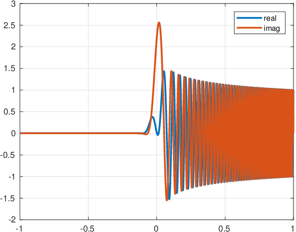
Refer to caption
Refer to caption
Refer to caption

TimingClose-up near the originApproximate solutiontime (secs) u ( x ) u ( x ) N x x

Fig. 11: (a) & (b) Approximate solution to the fractional Airy equation (153) with ε=10−4\varepsilon=10^{-4}. (c) Timings for building and solving the linear system for increasing degrees of freedom. Note that these scale linearly with the truncation length NN.

The first and second panels of Figure 11 show the real and imaginary parts of the solution for ε=10−4\varepsilon=10^{-4}, and we see behaviour qualitatively similar to that of the well-known classical Airy equation. Experimentally we find that an accuracy of 10−1010^{-10} requires around 750 degrees of freedom (i.e., N≈375N\approx 375), and forming and solving the almost-banded linear system representing the fractional differential operator and boundary conditions takes under a tenth of a second on a 2014 Desktop PC using the MATLAB implementation[15]. The third panel shows the computational times to form and solve the systems when the number degrees of freedom is artificially increased (as would be required for smaller values of ε\varepsilon). Using the Woodbury formula to solve the almost-banded linear system, we see that linear complexity is obtained. Finally, we note that this Riemann–Liouville FDE can be readily solved using ApproxFun [26] with just a few commands:

using ApproxFun S = Legendre() ⊕\oplus JacobiWeight(0.5, 0, Ultraspherical(1)) D1_5 = LeftDerivative(S, 1.5) x = Fun() u = [Dirichlet() ; 0.0001*im^1.5*D1_5 - x] \ [[0, 1], 0]
Table 1: ApproxFun code for solving the fractional Airy equation (153) with ε=10−4\varepsilon=10^{-4}.

Acknowledgements

We thank Daniel Hauer (U. Sydney) for discussions related to convergence in higher order norms, Marcus Webb (K.U. Leuven) for discussions on fractional differential equations, and Alex Townsend (Cornell) for some useful suggestions.

Appendix A Miscellaneous proofs

The following results are required in the proofs of Corollaries 2 and 3 in Sections 2.4 and 2.5, respectively.

Lemma A.24.

For any n>0n>0 and λ>0\lambda>0, the ultraspherical polynomials Cn(λ)​(x)C^{(\lambda)}_{n}(x) satisfy the relationship:

2​λ​(1+x)​(Cn(λ+1)​(x)−Cn−1(λ+1)​(x))=((n+1)​Cn+1(λ)​(x)+(n+2​λ)​Cn(λ)​(x)).2\lambda(1+x)\big(C_{n}^{(\lambda+1)}(x)-C_{n-1}^{(\lambda+1)}(x)\big)=\big((n+1)C_{n+1}^{(\lambda)}(x)+(n+2\lambda)C_{n}^{(\lambda)}(x)\big). (154)
Proof A.25.

Applying (17) to Cn(λ+1)​(x)C_{n}^{(\lambda+1)}(x) and Cn−1(λ+1)​(x)C_{n-1}^{(\lambda+1)}(x) gives, upon rearrangement,

(1+x)​(Cn(λ+1)​(x)−Cn−1(λ+1)​(x))=12​n+1n+λ+1​(Cn+1(λ+1)​(x)CLOSE−OPENCn−1(λ+1)​(x))+12​n+2​λn+λ​(Cn(λ+1)​(x)−Cn−2(λ+1)​(x)).\begin{array}[]{r c l}(1+x)\big(C_{n}^{(\lambda+1)}(x)-C_{n-1}^{(\lambda+1)}(x)\big)&\!\!\!\!=&\\ \frac{1}{2}\frac{n+1}{n+\lambda+1}\big(C_{n+1}^{(\lambda+1)}(x)&\!\!\!\!-&C_{n-1}^{(\lambda+1)}(x)\big)+\frac{1}{2}\frac{n+2\lambda}{n+\lambda}\big(C_{n}^{(\lambda+1)}(x)-C_{n-2}^{(\lambda+1)}(x)\big).\end{array} (155)

Applying (14) to each of the bracketed terms on the right-hand side and cancelling common terms gives the required result.

Corollary A.26.

The Legendre polynomials, Pn​(x)P_{n}(x), and the Chebyshev polynomials, Un​(x)U_{n}(x), satisfy

n⁡(Pn​(x)+Pn−1​(x))=(1+x)​(Cn−1(3/2)​(x)−Cn−2(3/2)​(x))n\big(P_{n}(x)+P_{n-1}(x)\big)=(1+x)\big(C_{n-1}^{(3/2)}(x)-C_{n-2}^{(3/2)}(x)\big) (156)

and

Un​(x)+(n+1)​Un−1​(x)=2​(1+x)​(Cn−1(2)​(x)−Cn−2(2)​(x)).U_{n}(x)+(n+1)U_{n-1}(x)=2(1+x)\big(C_{n-1}^{(2)}(x)-C_{n-2}^{(2)}(x)\big). (157)
Proof A.27.

Take n↦n−1n\mapsto n-1 with λ=12\lambda=\frac{1}{2} and λ=1\lambda=1 in (154), respectively.

Appendix B Convergence and stability results

B.1 Convergence

Note that the decompositions of the right-hand side and solution of (57) in the forms (58) and (64) are not unique, so the well-posedness of (66) is not immediate. However, the Schur complement of the (1,1)(1,1) block of (66) yields

(Q𝐏−σ2​I)​a¯\displaystyle\big(Q_{\mathbf{P}}-\sigma^{2}I\big)\underline{a} =\displaystyle= Q𝐔1/2​f¯−σ​e¯,\displaystyle Q^{1/2}_{\mathbf{U}}\underline{f}-\sigma\underline{e}, (158)
σ​b¯\displaystyle\sigma\underline{b} =\displaystyle= f¯−Q𝐏1/2​a¯,\displaystyle\underline{f}-Q_{\mathbf{P}}^{1/2}\underline{a},

where Q𝐏=Q𝐔1/2​Q𝐏1/2Q_{\mathbf{P}}=Q^{1/2}_{\mathbf{U}}Q^{1/2}_{\mathbf{P}} is the indefinite integral operator acting on the Legendre basis (recall (31)). The fact that Q𝐏Q_{\mathbf{P}} is banded along with the decaying properties of its entries leads to a proof of convergence whenever the original equation (57) is solvable in L2​[−1,1]L^{2}[-1,1].

Definition B.28.

Define the Banach space ℓλ2\ell_{\lambda}^{2} with norm

‖f¯‖ℓλ22=∑k=0∞(k+1)2​λ​fk2.\|\underline{f}\|_{\ell_{\lambda}^{2}}^{2}=\sum_{k=0}^{\infty}(k+1)^{2\lambda}f_{k}^{2}. (159)
Lemma B.29.

Let Ψ:=diag(2,23,25,27,…).\Psi:=\mathop{\operator@font diag}\nolimits\left(\sqrt{2},\sqrt{2\over 3},\sqrt{2\over 5},\sqrt{2\over 7},\ldots\right). If σ2\sigma^{2} is an ℓ2\ell^{2} eigenvalue of Q~𝐏:=Ψ​Q𝐏​Ψ−1\tilde{Q}_{\mathbf{P}}:=\Psi Q_{\mathbf{P}}\Psi^{-1}, then σ\sigma (as well as −σ-\sigma) is an L2​[−1,1]L^{2}[-1,1] eigenvalue of 𝒬1/2x−1{}_{-1}\mathcal{Q}_{x}^{1/2}.

Proof B.30.

Note that ‖Pn‖=22​n+1\|P_{n}\|=\sqrt{2\over 2n+1}, hence conjugating by Ψ\Psi recasts the operator to acting on expansions in the orthonormalized Legendre polynomials P~n​(x):=Pn​(x)​2​n+12\tilde{P}_{n}(x):=P_{n}(x)\sqrt{2n+1\over 2}. The assumption on σ2\sigma^{2} being an ℓ2\ell^{2} eigenvalue enforces that any eigenvector a¯\underline{a} of Q~𝐏\tilde{Q}_{\mathbf{P}} corresponds to the normalized Legendre coefficients of a function a⁡(x)a(x) in L2​[−1,1]L^{2}[-1,1], with norm ‖a¯‖ℓ2\|\underline{a}\|_{\ell^{2}}.

The entries of Q~𝐏\tilde{Q}_{\mathbf{P}} decay like 1/k1/k, see (31), which implies that Q~𝐏:ℓλ2→ℓλ+12\tilde{Q}_{\mathbf{P}}:\ell_{\lambda}^{2}\rightarrow\ell_{\lambda+1}^{2}. It follows immediately that a¯∈ℓλ2\underline{a}\in\ell_{\lambda}^{2} for all λ\lambda: a¯∈ℓλ2\underline{a}\in\ell_{\lambda}^{2} implies that a¯=σ−2​Q~𝐏​a¯∈ℓλ+12\underline{a}=\sigma^{-2}\tilde{Q}_{\mathbf{P}}\underline{a}\in\ell_{\lambda+1}^{2}. In particular, a¯∈ℓ1\underline{a}\in\ell^{1}. We can bound

‖1+x​Uk‖2=∫−11(1+x)​sin2⁡(k+1)​cos−1⁡xsin2⁡x​𝑑x=∫0π(1+cos⁡θ)​sin2⁡(k+1)​θsin⁡θ​𝑑θ≤2​π​(k+1)\|\sqrt{1+x}U_{k}\|^{2}=\int_{-1}^{1}(1+x){\sin^{2}(k+1)\cos^{-1}x\over\sin^{2}x}dx=\int_{0}^{\pi}(1+\cos\theta){\sin^{2}(k+1)\theta\over\sin\theta}d\theta\leq 2\pi(k+1) (160)

since Lagrange’s trigonometric identities ensure that

|sin⁡(k+1)​θsin⁡θ|≤k+1.\left|{\sin(k+1)\theta\over\sin\theta}\right|\leq k+1. (161)

Thus the O⁡(1/k)O(1/\sqrt{k}) decay in Q𝐏1/2​Ψ−1Q_{\mathbf{P}}^{1/2}\Psi^{-1} cancels the O⁡(k)O(\sqrt{k}) growth from ‖1+x​Uk‖\|\sqrt{1+x}U_{k}\|, and we have

‖(1+x​U0​(x),1+x​U1​(x),…)​Q𝐏1/2​Ψ−1​a¯‖≤C​‖a¯‖ℓ1<∞.\|\left(\sqrt{1+x}U_{0}(x),\sqrt{1+x}U_{1}(x),\ldots\right)Q_{\mathbf{P}}^{1/2}\Psi^{-1}\underline{a}\|\leq C\|\underline{a}\|_{\ell^{1}}<\infty. (162)

That is, the entries of b¯=σ−1​Q𝐏1/2​Ψ−1​a¯\underline{b}=\sigma^{-1}Q_{\mathbf{P}}^{1/2}\Psi^{-1}\underline{a} correspond to the second-kind Chebyshev coefficients of a function b⁡(x)b(x) such that 1+x​b​(x)\sqrt{1+x}b(x) is in L2​[−1,1]L^{2}[-1,1]. We therefore have an L2​[−1,1]L^{2}[-1,1] eigenvector a⁡(x)+1+x​b​(x)a(x)+\sqrt{1+x}b(x), satisfying:

𝒬x1/2​(a⁡(x)+1+x​b​(x))\displaystyle{\cal Q}_{x}^{1/2}(a(x)+\sqrt{1+x}b(x)) =𝒬x1/2​(𝐏⁡(x)​Ψ−1​a¯+𝐔1/2​(x)​b¯)\displaystyle={\cal Q}_{x}^{1/2}({\mathbf{P}}(x)\Psi^{-1}\underline{a}+{\mathbf{U}_{1/2}}(x)\underline{b})
=𝐔1/2​(x)​Q𝐏1/2​Ψ−1​a¯+𝐏⁡(x)​Q𝐔1/2​b¯\displaystyle={\mathbf{U}_{1/2}}(x)Q_{\mathbf{P}}^{1/2}\Psi^{-1}\underline{a}+{\mathbf{P}}(x)Q_{\mathbf{U}}^{1/2}\underline{b}
=σ​𝐔1/2​(x)​b¯+σ​𝐏​(x)​Ψ−1​a¯\displaystyle=\sigma{\mathbf{U}_{1/2}}(x)\underline{b}+\sigma{\mathbf{P}}(x)\Psi^{-1}\underline{a}
=σ⁡(a⁡(x)+1+x​b​(x))\displaystyle=\sigma(a(x)+\sqrt{1+x}b(x))
Lemma B.31.

If σI+−1𝒬x1/2\sigma I+_{-1}\mathcal{Q}_{x}^{1/2} is invertible in L2​[−1,1]L^{2}[-1,1] then σ2​I+Q~𝐏\sigma^{2}I+\tilde{Q}_{\mathbf{P}} is invertible in ℓλ2\ell_{\lambda}^{2} for all λ\lambda and in ℓ1\ell^{1}. If e¯,f¯∈ℓ1\underline{e},\underline{f}\in\ell^{1}, and a¯=(σ2​I+Q~𝐏)−1​(Q𝐔1/2​f¯−σ​e¯)\underline{a}=(\sigma^{2}I+\tilde{Q}_{\mathbf{P}})^{-1}(Q_{\mathbf{U}}^{1/2}\underline{f}-\sigma\underline{e}), then u⁡(x)=a⁡(x)+1+x​b​(x)u(x)=a(x)+\sqrt{1+x}b(x) satisfies

(σI+−1𝒬x1/2)u(x)=e(x)+1+xf(x)(\sigma I+_{-1}\mathcal{Q}_{x}^{1/2})u(x)=e(x)+\sqrt{1+x}f(x)

for e⁡(x)=𝐏⁡(x)​e¯e(x)=\mathbf{P}(x)\underline{e}, f​(x)=𝐔1/2​(x)​f¯f(x)=\mathbf{U}_{1/2}(x)\underline{f}, a⁡(x)=𝐏⁡(x)​a¯a(x)=\mathbf{P}(x)\underline{a} and b⁡(x)=σ−1​(f⁡(x)−𝐔1/2​(x)​Q𝐏1/2​a¯)b(x)=\sigma^{-1}(f(x)-\mathbf{U}_{1/2}(x)Q_{\mathbf{P}}^{1/2}\underline{a}).

Proof B.32.

The decay in the entries of Q~𝐏\tilde{Q}_{\mathbf{P}} and bandedness imply that ‖PN​Q~𝐏−Q~𝐏‖ℓλ2→0\|P_{N}\tilde{Q}_{\mathbf{P}}-\tilde{Q}_{\mathbf{P}}\|_{\ell_{\lambda}^{2}}\rightarrow 0: Q~𝐏\tilde{Q}_{\mathbf{P}} is compact in ℓλ2\ell_{\lambda}^{2} (and by a similar argument, in ℓ1\ell^{1}). Compactness guarantees that the operator only has discrete eigenvalues. However, the previous lemma ensures that if σI+−1𝒬x1/2\sigma I+_{-1}\mathcal{Q}_{x}^{1/2} is invertible in L2​[−1,1]L^{2}[-1,1], then σ2\sigma^{2} is not an ℓ2\ell^{2} eigenvalue of Q~𝐏\tilde{Q}_{\mathbf{P}}, and hence σ2​I+Q~𝐏\sigma^{2}I+\tilde{Q}_{\mathbf{P}} is invertible in ℓ2\ell^{2}. But any ℓ2\ell^{2} eigenvector is an eigenvector in ℓλ2\ell_{\lambda}^{2} for all λ≥0\lambda\geq 0 (and in ℓ1\ell^{1}) as Q~𝐏\tilde{Q}_{\mathbf{P}} induces additional decay, and trivially, any ℓλ2\ell_{\lambda}^{2} eigenvector is automatically an ℓ2\ell^{2} eigenvector. Thus we know that σ2\sigma^{2} is also not an ℓλ2\ell_{\lambda}^{2} (or ℓ1\ell^{1}) eigenvalue, and the operator is invertible.

Therefore, if e¯,f¯∈ℓ1\underline{e},\underline{f}\in\ell^{1} then a¯∈ℓ1\underline{a}\in\ell^{1}, hence (by the logic of the previous lemma) a⁡(x)+1+x​b​(x)∈L2​[−1,1]a(x)+\sqrt{1+x}b(x)\in L^{2}[-1,1]. We have thus constructed the unique L2​[−1,1]L^{2}[-1,1] solution of (σI+−1𝒬x1/2)u(x)=e(x)+1+xf(x)(\sigma I+_{-1}\mathcal{Q}_{x}^{1/2})u(x)=e(x)+\sqrt{1+x}f(x)

We now consider the finite section approximation of (66), i.e., we define the projection operator PN:ℓ2→ℝNP_{N}:\ell^{2}\rightarrow\mathbb{R}^{N} and consider the 2​N×2​N2N\times 2N finite section approximation

(σ​INPN​Q𝐔1/2​PN⊤PN​Q𝐏1/2​PN⊤σ​IN)​(a¯Nb¯N)=(PN​e¯PN​f¯).\left(\begin{array}[]{c c}\sigma I_{N}&P_{N}Q_{\mathbf{U}}^{1/2}P_{N}^{\top}\\ P_{N}Q_{\mathbf{P}}^{1/2}P_{N}^{\top}&\sigma I_{N}\end{array}\right)\left(\begin{array}[]{c}\underline{a}_{N}\\ \underline{b}_{N}\end{array}\right)=\left(\begin{array}[]{c}P_{N}\underline{e}\\ P_{N}\underline{f}\end{array}\right). (163)

This leads to an approximation

a⁡(x)≈aN​(x)=𝐏⁡(x)​a¯Nb⁡(x)≈bN​(x)=σ−1​𝐔​(x)​(PN​f¯−Q𝐏1/2​a¯N)u⁡(x)≈uN​(x)=aN​(x)+1+x​bN​(x).\begin{array}[]{r c l c l}a(x)&\approx&a_{N}(x)&=&{\mathbf{P}}(x)\underline{a}_{N}\\ b(x)&\approx&b_{N}(x)&=&\sigma^{-1}{\mathbf{U}}(x)(P_{N}\underline{f}-Q_{\mathbf{P}}^{1/2}\underline{a}_{N})\\ u(x)&\approx&u_{N}(x)&=&a_{N}(x)+\sqrt{1+x}b_{N}(x).\end{array} (164)
Theorem B.33.

If σI+−1𝒬x1/2\sigma I+_{-1}\mathcal{Q}_{x}^{1/2} is invertible in L2​[−1,1]L^{2}[-1,1] and e¯\underline{e}, f¯\underline{f} are in ℓ1\ell^{1}, then the finite section approximation to (158) uNu_{N} converges to the true solution of (57) in L2​[−1,1]L^{2}[-1,1].

Proof B.34.

Note that, because Q𝐏1/2Q_{\mathbf{P}}^{1/2} is upper triangular and Q𝐔1/2Q_{\mathbf{U}}^{1/2} is lower triangular, we have

PN​Q𝐔1/2​PN⊤​PN​Q𝐏1/2​PN⊤=PN​Q𝐔1/2​Q𝐏1/2​PN⊤=PN​Q𝐏​PN⊤.P_{N}Q_{\mathbf{U}}^{1/2}P_{N}^{\top}P_{N}Q_{\mathbf{P}}^{1/2}P_{N}^{\top}=P_{N}Q_{\mathbf{U}}^{1/2}Q_{\mathbf{P}}^{1/2}P_{N}^{\top}=P_{N}Q_{\mathbf{P}}P_{N}^{\top}. (165)

It follows that a¯N\underline{a}_{N} is also a solution to the n×nn\times n finite section of (158):

PN​(Q𝐏−σ2​I)​PN⊤​a¯N=PN​(Q𝐔1/2​f¯−σ​e¯).P_{N}(Q_{\mathbf{P}}-\sigma^{2}I)P_{N}^{\top}\underline{a}_{N}=P_{N}(Q_{\mathbf{U}}^{1/2}\underline{f}-\sigma\underline{e}). (166)

If the condition of this theorem holds, then by the previous lemma, σ2\sigma^{2} is not an eigenvalue of Q~𝐏\tilde{Q}_{\mathbf{P}} . Q~𝐏\tilde{Q}_{\mathbf{P}} is a compact operator on ℓ1\ell^{1}, therefore the finite-section approximation a¯N\underline{a}_{N} converges to a¯\underline{a} in an ℓ1\ell^{1} sense (this follows from a Neumann series argument, see e.g., [27, Theorem 4.5]). This implies convergence of aN​(x)a_{N}(x) to a⁡(x)a(x) in L2​[−1,1]L^{2}[-1,1] and convergence of bN​(x)b_{N}(x) to b⁡(x)b(x) in L2​[−1,1]L^{2}[-1,1], thence uN​(x)u_{N}(x) converges to u⁡(x)u(x) in L2​[−1,1]L^{2}[-1,1].

Corollary B.35.

If e¯,f¯∈ℓλ2\underline{e},\underline{f}\in\ell_{\lambda}^{2} then the finite section approximation converges in ℓλ2\ell_{\lambda}^{2}. If this condition holds for all λ\lambda, then uNu_{N} converges in L2​[−1,1]L^{2}[-1,1] at a spectrally fast rate. Similarly, if e¯,f¯\underline{e},\underline{f} decay exponentially, then uNu_{N} converges in L2​[−1,1]L^{2}[-1,1] exponentially fast.

Proof B.36.

The first statement follows from the operator being a compact perturbation of the identity in all ℓλ2\ell_{\lambda}^{2} spaces, hence the same argument as Theorem B.33 applies. The second statement follows from relating convergence in ℓλ2\ell_{\lambda}^{2} to fast convergence in ℓ1\ell^{1}. The exponentially fast convergence follows similarly by adapting the results to the exponentially weighted norm ∑k=0∞|Rk​fk|2\sqrt{\sum_{k=0}^{\infty}|R^{k}f_{k}|^{2}}.

B.2 Stability

Unfortunately, solvability of the resulting equation is not the only issue: we must also consider conditioning. Now, v⁡(x)=ex/σ2v(x)=e^{x/\sigma^{2}} is the solution to 𝒬u(x)−σ2u(x)=e−1/σ2\mathcal{Q}u(x)-\sigma^{2}u(x)=e^{-1/\sigma^{2}}, hence, for σ≪1\sigma\ll 1, v⁡(x)v(x) is approximately in the kernel of 𝒬​u​(x)−σ2​I\mathcal{Q}u(x)-\sigma^{2}I. Therefore, we should expect the solution of the above system, and hence the system (66) to be ill-conditioned when σ≪1\sigma\ll 1. Indeed, the pseudo-spectral plot of the two (truncated) linear systems in Figure 12 confirms this.

Refer to caption
Refer to caption
Fig. 12: Left: Pseudospectra (computing using EigTool [41]) of the operator Q1/2Q_{1/2} truncated to a 200×200200\times 200 matrix. Right: The same for (66) with σ=0\sigma=0.

Decreasing σ\sigma in this way is equivalent to a change of variables from [−1,1][-1,1] to a longer ‘time’ domain (if we consider the independent variable as time). In particular, let y=1σ2​x+cy=\frac{1}{\sigma^{2}}x+c and u⁡(x)=v⁡(y)u(x)=v(y), then substituting to (5) we find

𝒬x1/2−1​u​(x)=σ−α​𝒬y1/2​v​(y).\ {}_{-1}\mathcal{Q}^{1/2}_{x}u(x)=\sigma\ _{-\alpha}\mathcal{Q}^{1/2}_{y}v(y). (167)

Investigating the singular values of the operator suggests that as σ→0\sigma\rightarrow 0 it is only a single singular value that decays to zero and that it might be possible to regularise the problem. However, this is beyond the scope of the current paper and we avoid this limiting case for now.

References

  • [1] B. K. Alpert and V. Rokhlin, A fast algorithm for the evaluation of Legendre expansions, SIAM Journal on Scientific and Statistical Computing, 12 (1991), pp. 158–179.
  • [2] G. E. Andrews, R. Askey, and R. Roy, Special functions, vol. 71, Cambridge University Press, 1999.
  • [3] J. L. Aurentz and L. N. Trefethen, Chopping a chebyshev series, ACM Transactions on Mathematical Software, 43 (2017), p. 33.
  • [4] R. L. Bagley and P. J. Torvik, Fractional calculus – a different approach to the analysis of viscoelastically damped structures, 1983.
  • [5]  , On the appearance of the fractional derivative in the behavior of real materials, 1984.
  • [6] E. G. Bajlekova, Fractional evolution equations in Banach spaces, ProQuest LLC, Ann Arbor, MI, 2001. Thesis (Dr.)–Technische Universiteit Eindhoven (The Netherlands).
  • [7] S. Chen, J. Shen, and L.-L. Wang, Generalized Jacobi functions and their applications to fractional differential equations, Math. Comp., 85 (2016), pp. 1603–1638.
  • [8] O. Christensen, An Introduction to Frames and Riesz Bases, Birkhauser, 2003.
  • [9] M. Cui, Compact finite difference method for the fractional diffusion equation, Journal of Computational Physics, 228 (2009), pp. 7792–7804.
  • [10] M. Dalir and M. Bashour, Applications of fractional calculus, Applied Mathematical Sciences, 4 (2010), pp. 1021–1032.
  • [11] W. Deng, Finite element method for the space and time fractional Fokker–Planck equation, SIAM Journal on Numerical Analysis, 47 (2008), pp. 204–226.
  • [12] NIST Digital Library of Mathematical Functions. http://dlmf.nist.gov/, Release 1.0.10 of 2015-08-07. Online companion to [25].
  • [13] T. A. Driscoll, N. Hale, and L. N. Trefethen, Chebfun Guide, Pafnuty Publications, 2014.
  • [14] N. Ford, J. Xiao, and Y. Yan, A finite element method for time fractional partial differential equations, Fractional Calculus and Applied Analysis, 14 (2011), pp. 454–474.
  • [15] N. Hale, Companion code to this paper. https://github.com/nickhale/fracspec_code. Last accessed 17 Oct 2016.
  • [16] N. Hale and A. Townsend, A fast, simple, and stable Chebyshev–Legendre transform using an asymptotic formula, SIAM J. Sci. Comput., 36 (2014), pp. A148–A167.
  • [17] R. Hilfer, Applications of Fractional Calculus in Physics, World Scientific, 2000.
  • [18] H. Li and Y. Xu, Spectral approximation on the unit ball, SIAM J. Numer. Anal., 52 (2014), pp. 2647–2675.
  • [19] X. Li and C. Xu, A space-time spectral method for the time fractional diffusion equation, SIAM J. Numer. Anal., 47(3) (2009), p. 2108–2131.
  • [20] F. Liu, V. Anh, and I. Turner, Numerical solution of the space fractional Fokker–Planck equation, Journal of Computational and Applied Mathematics, 166 (2004), pp. 209–219.
  • [21] R. L. Magin, Fractional Calculus in Bioengineering, Begell House Redding, 2006.
  • [22]  , Fractional calculus models of complex dynamics in biological tissues, Computers & Mathematics with Applications, 59 (2010), pp. 1586–1593.
  • [23] M. M. Meerschaert and C. Tadjeran, Finite difference approximations for two-sided space-fractional partial differential equations, Applied numerical mathematics, 56 (2006), pp. 80–90.
  • [24] K. B. Oldham, Fractional differential equations in electrochemistry, Advances in Engineering Software, 41 (2010), pp. 9–12.
  • [25] F. W. J. Olver, D. W. Lozier, R. F. Boisvert, and C. W. Clark, eds., NIST Handbook of Mathematical Functions, Cambridge University Press, New York, NY, 2010. Print companion to [12].
  • [26] S. Olver, ApproxFun.jl v0.7, https://github.com/approxfun/approxfun.jl.
  • [27] S. Olver and A. Townsend, A fast and well-conditioned spectral method, SIAM Rev., 55 (2013), pp. 462–489.
  • [28] S. Olver and A. Townsend, A practical framework for infinite-dimensional linear algebra, in Proceedings of the 1st First Workshop for High Performance Technical Computing in Dynamic Languages, 2014, pp. 57–62.
  • [29] M. D. Ortigueira and J. T. Machado, Fractional calculus applications in signals and systems, Signal Processing, 86 (2006), pp. 2503 – 2504. Special Section: Fractional Calculus Applications in Signals and Systems.
  • [30] A. D. Polyanin and A. V. Manzhirov, Handbook of integral equations, Chapman & Hall/CRC, Boca Raton, FL, second ed., 2008.
  • [31] M. Riesz, L’intégrale de Riemann–Liouville et le problème de Cauchy, Acta Math., 81 (1949), pp. 1–223.
  • [32] J. Sabatier, O. P. Agrawal, and J. T. Machado, Advances in Fractional Calculus, vol. 4, Springer, 2007.
  • [33] E. Scalas, R. Gorenflo, and F. Mainardi, Fractional calculus and continuous-time finance, Physica A: Statistical Mechanics and its Applications, 284 (2000), pp. 376–384.
  • [34] H. Sheng, Y. Chen, and T. Qiu, Fractional Processes and Fractional-order Signal Processing: Techniques and Applications, Springer Science & Business Media, 2011.
  • [35] R. M. Slevinsky and S. Olver, A fast and well-conditioned spectral method for singular integral equations, J. Comput. Phys., 332 (2017), pp. 290–315.
  • [36] G. W. Stewart, Afternotes goes to graduate school, Society for Industrial and Applied Mathematics (SIAM), Philadelphia, PA, 1998. Lectures on advanced numerical analysis.
  • [37] A. Townsend and S. Olver, The automatic solution of partial differential equations using a global spectral method, J. Comput. Phys., 299 (2015), pp. 106–123.
  • [38] A. Townsend, M. Webb, and S. Olver, Fast polynomial transforms based on Toeplitz and Hankel matrices, Maths Comp., (2016). To appear.
  • [39] L. N. Trefethen, Approximation theory and approximation practice, Society for Industrial and Applied Mathematics (SIAM), Philadelphia, PA, 2013.
  • [40] G. M. Vasil, K. J. Burns, D. Lecoanet, S. Olver, B. P. Brown, and J. S. Oishi, Tensor calculus in polar coordinates using Jacobi polynomials, J. Comp. Phys., 325 (2016), pp. 53–73.
  • [41] T. G. Wright., Eigtool, 2002.
  • [42] S. B. Yuste and L. Acedo, An explicit finite difference method and a new von Neumann-type stability analysis for fractional diffusion equations, SIAM Journal on Numerical Analysis, 42 (2005), pp. 1862–1874.
  • [43] M. Zayernouri and G. E. Karniadakis, Fractional spectral collocation method, SIAM J. Sci. Comput., 36 (2014), pp. A40–A62.
  • [44] L. Zhao, W. Deng, and J. S. Hesthaven, Spectral methods for tempered fractional differential equations, ArXiv e-print: 1603.06511, (2016).