跳到论文正文
W Papers独立论文阅读器 arXiv:1611.07974 论文正文 计算阅读时间 · 0%
引用这篇论文根据当前论文元数据生成,正式投稿前建议核对。


License: arXiv.org perpetual non-exclusive license
arXiv:1611.07974v3 [hep-ph] 16 Feb 2018

A Unified Hidden-Sector Electroweak Model, Para-photons and the X-boson

M. J. Neves a Email: mariojr@ufrrj.br, helayel@cbpf.br    and J. A. Helayël-Neto b Affiliation: aDepartamento de Física,
Universidade Federal Rural do Rio de Janeiro
BR 465-07, 23890-971, Seropédica, Rio de Janeiro, Brazil

bCentro Brasileiro de Pesquisas Físicas (CBPF),
Rua Dr. Xavier Sigaud 150, Urca,
CEP 22290-180, Rio de Janeiro, Brazil

August 24, 2026
Abstract

Our contribution sets out to investigate the phenomenology of a gauge model based on an S​UL​(2)×UR​(1)J×U​(1)KSU_{L}(2)\times U_{R}(1)_{J}\times U(1)_{K}-symmetry group. The model can accommodate in its distinct phases - by virtue of different symmetry-breaking patterns - a candidate to a heavy Z′Z^{\prime}-boson at the TeV-scale and the recently discussed 17​MeV17\,\mbox{MeV} X-boson that may bring about a new physics at the MeV-scale. Furthermore, the para-photon of the dark matter sector and the candidate to the so-called dark photon can also be described in the scenario we are endeavoring to set up in this paper. In the Z′Z^{\prime}-scenario, the extended Higgs sector introduces a heavy scalar whose mass lies in the region 1.2−3.7​TeV1.2-3.7\,\mbox{TeV}, while that the lower energy scale scenario presents a light scalar with mass in the interval 1.9−19​GeV1.9-19\,\mbox{GeV}. The fermionic sector includes an exotic candidate to dark matter that mixes with the right-neutrino component in the Higgs sector, so that the whole field content yields the cancellation of the U(1)-anomaly. The masses are fixed according to the particular way the symmetry breaking takes place. In view of the possible symmetry breakdown patterns, we study the phenomenological implications in both scenarios of high- and low-energy scales. As examples, we consider the scattering of Standard Model matter into dark sector constituents intermediated by the Z′Z^{\prime}-boson in the TeV-scale, and the corresponding scattering intermediated by a lightest boson in the lower scale physics. Furthermore, we obtain the magnetic dipole momentum (MDM) of the exotic fermion and the transition MDM due to the mixing with the right-neutrino.

Keywords
Physics beyond Standard Model, Hidden particles, Dark matter.

1 Introduction

The search for new particles and interactions beyond the Standard Model (SM) has been challenging High-Energy Physics, both Theoretical and Experimental, over the recent decades. The results from the LHC’s ATLAS- and CMS-Collaborations may point to the existence of a (new) fifth interaction [1, 2]. Analysing data of p​ppp-collisions at a center-of-mass energy scale of s=13​TeV\sqrt{s}=13\,\mbox{TeV} has revealed peaks of masses that may correspond to the hypothetical heavy W′W^{\,\prime}- and Z′Z^{\,\prime}-bosons [3, 4], which may be an evidence for new Physics communicated from very high energies to the TeV-scale. We should keep in mind that the introduction of an extra Higgs may be needed to explain the heavy mass of the new bosons at the TeV-scale. These masses are associated with a new range of vacuum expectation values (VEVs) of supplementary Higgs scalars.

A well-known model in this direction is based on an S​UL​(2)×S​UR​(2)×U​(1)B−LSU_{L}(2)\times SU_{R}(2)\times U(1)_{B-L}-gauge symmetry [6, 7, 8, 9, 10, 11, 12, 13]. The extra S​UR​(2)SU_{R}(2)-subgroup is introduced to account for the hypothetical W′W^{\,\prime}- and Z′Z^{\,\prime}-bosons, besides the already known W±W^{\pm}- and Z0Z^{0}-weak mediators of the Glashow-Salam-Weinberg (GSW) model. The right-handed sector also introduces fermion doublets with a charged lepton and its associated neutrino of right chirality. Two scalar doublets constitute the Higgs sector responsible for the chain of symmetry breakings. The first doublet is introduced to break the S​UR​(2)×U​(1)B−LSU_{R}(2)\times U(1)_{B-L}-gauge symmetry at the scale set up by the VEV uu, above the SM Electroweak scale u>v=246​GeVu>v=246\,\mbox{GeV}. As a consequence, the hypercharge, YY, appears as a combination of generators of S​UR​(2)×U​(1)B−LSU_{R}(2)\times U(1)_{B-L}. Next, the Standard Model Higgs breaks the remaining gauge symmetry down to the eletromagnetic Abelian symmetry, U​(1)e​mU(1)_{em}. Therefore, the recent CMS simulation indicates that the estimate for masses of hypothetical W′W^{\prime} and Z′Z^{\prime} is around the 2​TeV2\,\mbox{TeV} [3, 4].

The well-known model in the literature that describes only the Z′Z^{\prime}-heavy boson is based on the gauge symmetry S​UL​(2)×UY​(1)×U​(1)B−LSU_{L}(2)\times U_{Y}(1)\times U(1)_{B-L} [14, 15, 16], which includes a U⁡(1)U(1)-extra group in the GSW model. The gauge sector has just one extra boson, while the Higgs is extended to include a doublet and a singlet, or bi-doublets of scalars fields. The fermion sector is enlarged to guarantee anomaly cancellation; for example, the introduction of right-neutrinos components and exotic fermions that could be candidates to dark matter content.

In 2016, in a particular Nuclear Physics experiment, anomalies in the decay of the excited state of 8​Be∗8\,\mbox{Be}^{\ast} to its ground state has suggested the existence of a new neutral boson, called XX, through the decay mode 8​Be∗→8​Be+X8\,\mbox{Be}^{\ast}\rightarrow 8\,\mbox{Be}+X [17]. The XX-boson immediately decays into an electron-positron pair X→e++e−X\rightarrow e^{+}\,+\,e^{-}. It is a vector-type spin-1 neutral particle, with mass around mX=17​MeVm_{X}=17\,\mbox{MeV} that mixes with the SM photon through a kinetic term. Its origin could, in principle, be traced back to an extra gauge symmetry, U​(1)XU(1)_{X}, in addition to the symmetries of the SM. The discovery of the X-boson may be pointing to the existence of a fifth fundamental interaction in Nature. This is an interesting scenario in which the hypothetical fifth interaction would be accessible at the MeV-scale.

The effective Lagrangian proposed to describe this extra XX-boson is given below [20]

ℒe​f​f=−14​Fμ​ν 2−14​Xμ​ν 2+χ2​Xμ​ν​Fμ​ν+12​mX 2​Xμ 2−Jμ​Xμ,{\cal L}_{eff}=-\frac{1}{4}\,F_{\mu\nu}^{\,2}-\frac{1}{4}\,X_{\mu\nu}^{\,2}+\frac{\chi}{2}\,X_{\mu\nu}F^{\mu\nu}+\frac{1}{2}\,m_{X}^{\,2}\,X_{\mu}^{\,2}-J_{\mu}X^{\mu}\,, (1.1)

where JμJ^{\mu} is the current weakly coupled to XμX^{\mu}

Jμ=∑Ψ=e,u,d,…e​χΨ​Ψ¯​γμ​Ψ,\displaystyle J^{\mu}=\!\!\!\!\!\sum_{\Psi\,=\,e\,,\,u\,,\,d\,,\,...}\!\!\!\!e\,\chi_{\Psi}\,\bar{\Psi}\,\gamma^{\mu}\,\Psi\;, (1.2)

with Ψ\Psi standing for any fermion of the SM. This vector current exhibits a protophobic character described by the χp\chi_{p}-parameter whose magnitude for the proton and neutron satisfies the condition χp≪χn\chi_{p}\ll\chi_{n}, whenever the XX-boson interacts with the nucleon. We list some estimates of χΨ\chi_{\Psi} for the fermions of the SM, following the phenomenology of the XX-boson [18] :

2×10⁻⁴<\displaystyle 2\times 10^{-4}< |χe|\displaystyle|\chi_{e}| <1.4×10⁻³,\displaystyle<1.4\times 10^{-3}\;,
|χn|\displaystyle|\chi_{n}| <\displaystyle< 2.5×10⁻²,\displaystyle 2.5\times 10^{-2}\;,
|χν​χe|\displaystyle\sqrt{|\chi_{\nu}\,\chi_{e}|} ≲\displaystyle\lesssim 7×10⁻⁵.\displaystyle 7\times 10^{-5}\;. (1.3)

while that for the uu- and dd-quarks, the extreme protophobic limit, (χp=0)(\chi_{p}=0), parameterizes χu\chi_{u} and χd\chi_{d} as it follows below :

χu\displaystyle\chi_{u} =\displaystyle= −χn3≃± 3.7×10⁻³\displaystyle-\frac{\chi_{n}}{3}\simeq\pm\,3.7\times 10^{-3}
χd\displaystyle\chi_{d} =\displaystyle= +2​χn3≃∓ 7.4×10⁻³.\displaystyle+\frac{2\,\chi_{n}}{3}\simeq\mp\,7.4\times 10^{-3}\;. (1.4)

The XμX^{\mu}-boson can also have a chiral interaction with the SM leptons via an axial current, see [19]. For a complete review on the anomaly in Beryllium decays, see [20]. Still in the Lagrangian (1.1), the parameter χ\chi mixes the XμX^{\mu}-boson with the usual electromagnetic (EM) photon, AμA^{\mu}, where Xμ​ν=∂μXν−∂νXμX^{\mu\nu}=\partial^{\mu}X^{\nu}-\partial^{\nu}X^{\mu} is the field-strength tensor for XμX^{\mu}, and Fμ​ν=∂μAν−∂νAμF^{\mu\nu}=\partial^{\mu}A^{\nu}-\partial^{\nu}A^{\mu}, the corresponding tensor field for the photon. It is clear that the massive term spoils the U​(1)XU(1)_{X}-symmetry, and the Lagrangian exhibits only EM gauge symmetry, Ue​m​(1)U_{em}(1). Thus, the presence of the mass in (1.1) motivates us to search for a physical mechanism that underlies its generation. There has emerged an important connection between the U​(1)XU(1)_{X}-symmetry and dark matter in a model with spontaneous symmetry breaking (SSB); for that, see the recent paper of Ref. [23].

In another context, the search for single photons in 53​fb−153\,\mbox{fb}^{-1}, in the e+​e−e^{+}\,e^{-} CM-collision with the production of a spin-1 particle, A′A^{\prime}, referred to as dark photon, is associated to the process e+​e−→γ​A′e^{+}\,e^{-}\,\rightarrow\,\gamma\,A^{\prime} [24]. Immediately, the dark photon decays into invisible fermion matter A→ζ¯​ζA\,\rightarrow\,\bar{\zeta}\,\zeta, that can be a candidate to dark matter constituent. The A′A^{\prime} dark-photon has therefore a similar phenomenology to the XX-Boson, with a kinetic mixing of order 10−310^{-3}, with the EM photon. The dominant decay mode for the lowest-mass of the ζ\zeta-state fixes the condition mA′> 2​mζm_{A^{\prime}}\,>\,2\,m_{\zeta}, considering that the mA′m_{A^{\prime}}-dark-photon mass is bounded from above by mA′≤8​GeVm_{A^{\prime}}\leq 8\,\mbox{GeV}.

In the literature, there is also a great deal of interest in the activity related to the phenomenology of hidden sector para-photons [25, 26, 27]. The para-photon is a neutral vector boson with a sub-eV mass and with the property of electromagnetic interactions with coupling constants referred to as millicharges. The para-photons are characterized by a mixed mass term with the photon and they appear with an extra U⁡(1)U(1) gauge factor in the full symmetry group. The particles like the boson-X, dark-photon or para-photon that interact with a current like (1.2) are known in the literature as Weakly Interacting Massive Particles (WIMP). This idea connects the matter content of the SM with possible new dark matter particles via scattering processes.

In the present paper, we re-assess the S​UL​(2)×UR​(1)J×U​(1)KSU_{L}(2)\times U_{R}(1)_{J}\times U(1)_{K} model whose spontaneous symmetry breaking (SSB) mechanism can be applied in two scenarios: with a higher (TeV) or a lower (MeV) energy scale; for details, consult [28]. We study its phenomenology such that the new bosons, Z′Z^{\prime} or XX, can connect the world of SM particles with dark matter particles in particular scattering processes. Furthermore, the introduction of a mixing involving a Dirac right-neutrino component with exotic fermions, i. e., heavy and neutral fermions, can unveil new magnetic properties of these new fermions. We pursue this investigation and we obtain the transition Magnetic Dipole Momentum (MDM) and the MDM for the exotic fermion that depend on its mass, as it happens in the neutrino case. Sectors of fermions and scalar bosons are introduced with quantum numbers consistent with the gauge invariance and the chiral anomalies associated to the Abelian sectors cancel out.

The organization of this paper follows the outline below: in Section II, we review the Z′Z^{\prime}-model based on an S​UL​(2)×UR​(1)J×U​(1)KSU_{L}(2)\times U_{R}(1)_{J}\times U(1)_{K}-symmetry presented in details in [28]. In Section III, we study in details the diagonalization of the dark fermion and right-neutrino sector. Section IV is presented in three subsections, where we study the Z′Z^{\prime}-decay modes into fermions, the decay modes of the extra Higgs and the scattering processes quark-quark and dark fermion mediated by the Z′Z^{\prime} particle. In the Section V, we obtain the transition MDM and the MDM of the dark fermion. Section VI contains a review of SSB in association with the XX-boson and the dark photon scenario of [28]. In Section VII, we study the decay modes of the dark photon (first subsection) and we work out the scattering process for the cascade effect e+​e−→X→ζ¯​ζe^{+}\,e^{-}\,\rightarrow\,X\,\rightarrow\,\bar{\zeta}\,\zeta (second subsection). The third subsection is dedicated to form factor calculations in the correction to the QED vertex due to the axial interaction of the X-boson with the leptons of the SM. Finally, our Concluding Comments are cast in Section VIII.

2 A review of the Z′Z^{\prime}-model

In this Section, we present a short review of the Z′Z^{\prime}-model; the details may be found in the work of Ref. [28]. Here, we introduce the model in the renormalizable RξR_{\xi}-gauge. The sector of fermions and gauge fields of the model S​UL​(2)×UR​(1)J×U​(1)KSU_{L}(2)\times U_{R}(1)_{J}\times U(1)_{K}-model is described by the Lagrangian below :

ℒf=Ψ¯L​i/D​ΨL+Ψ¯R​i/D​ΨR+ν¯i​R​i/D​νi​R+ζ¯i​i/D​ζi,{\cal L}_{f}=\bar{\Psi}_{L}\,i\,\,/\penalty{\!\!\!\!D}\,\Psi_{L}+\bar{\Psi}_{R}\,i\,\,/\penalty{\!\!\!\!D}\,\Psi_{R}+\bar{\nu}_{iR}\,i\,\,/\penalty{\!\!\!\!D}\,\nu_{iR}+\bar{\zeta}_{i}\,i\,\,/\penalty{\!\!\!\!D}\,\zeta_{i}\;, (2.1)

and

ℒg​a​u​g​e=−12​tr​(Fμ​ν 2)−14​Bμ​ν 2−14​Cμ​ν 2.{\cal L}_{gauge}=-\frac{1}{2}\,\mbox{tr}\left(F_{\mu\nu}^{\;2}\right)-\frac{1}{4}\,B_{\mu\nu}^{\;2}-\frac{1}{4}\,C_{\mu\nu}^{\;2}\;. (2.2)

The slashed notation corresponds to the contraction of the covariant derivatives with the usual Dirac matrices. The covariant derivatives acting on the fermions of the model are cast according to:

Dμ​ΨL\displaystyle D_{\mu}\Psi_{L} =\displaystyle= (∂μ+igAμaσa2+iJLg′Bμ+iKLg′′Cμ)ΨL,\displaystyle\left(\partial_{\mu}+i\,g\,A_{\mu}^{\,a}\,\frac{\sigma^{a}}{2}+i\,J_{L}\,g^{\prime}\,B_{\mu}+i\,K_{L}\,g^{\prime\prime}\,C_{\mu}\!\right)\!\Psi_{L}\;,
Dμ​ΨR\displaystyle D_{\mu}\Psi_{R} =\displaystyle= (∂μ+iJRg′Bμ+iKRg′′Cμ)ΨR,\displaystyle\left(\phantom{\frac{1}{2}}\!\!\!\!\partial_{\mu}+i\,J_{R}\,g^{\prime}\,B_{\mu}+i\,K_{R}\,g^{\prime\prime}\,C_{\mu}\right)\Psi_{R}\;,
Dμ​νi​R\displaystyle D_{\mu}\nu_{iR} =\displaystyle= (∂μ+iJνRg′Bμ+iKνRg′′Cμ)νi​R,\displaystyle\left(\phantom{\frac{1}{2}}\!\!\!\!\partial_{\mu}+i\,J_{\nu_{R}}\,g^{\prime}\,B_{\mu}+i\,K_{\nu_{R}}\,g^{\prime\prime}\,C_{\mu}\right)\nu_{iR}\;,
Dμ​ζi\displaystyle D_{\mu}\zeta_{i} =\displaystyle= (∂μ+iJζg′Bμ+iKζg′′Cμ)ζi,\displaystyle\left(\phantom{\frac{1}{2}}\!\!\!\!\partial_{\mu}+i\,J_{\zeta}\,g^{\prime}\,B_{\mu}+i\,K_{\zeta}\,g^{\prime\prime}\,C_{\mu}\right)\zeta_{i}\;, (2.3)

where Aμ​a={Aμ​ 1,Aμ​ 2,Aμ​ 3}A^{\mu\,a}\!=\!\left\{\,A^{\mu\,1}\,,\,A^{\mu\,2}\,,\,A^{\mu\,3}\,\right\} are the gauge fields of S​UL​(2)SU_{L}(2), BμB^{\mu} is the Abelian gauge field of UR​(1)JU_{R}(1)_{J}, and CμC^{\mu} the similar one to U​(1)KU(1)_{K}. Here, we have chosen the symbol JJ to represent the generator of UR​(1)JU_{R}(1)_{J}, KK is the generator of U​(1)KU(1)_{K}, the generators of S​UL​(2)SU_{L}(2) are the Pauli matrices σa2​(a=1,2,3)\frac{\sigma^{a}}{2}\,(a=1,2,3), and gg, g′g^{\,\prime} and g′′g^{\,\prime\prime} are dimensionless gauge couplings. The fermionic field content is given in the sequel. The notation ΨL\Psi_{L} indicates the usual doublet of neutrinos/leptons Li=(νi​ℓi)LtL_{i}=(\nu_{i}\,\,\,\ell_{i})_{L}^{t}, or quarks Qi​LQ_{iL} (i=1,2,3)(i=1,2,3) left-handed of the SM, it turn out in the fundamental representation of S​UL​(2)SU_{L}(2). The label ℓi​L=(eL,μL,τL)\ell_{iL}=\left(\,e_{L}\,,\,\mu_{L}\,,\,\tau_{L}\,\right) indicates the leptons family displayed in the doublet, and the νi​L\nu_{iL}-label for neutrinos is defined by νi​L=(νeL,νμL,ντL)\nu_{iL}=(\nu_{e_{L}},\nu_{\mu_{L}},\nu_{\tau_{L}}). The ΨR\Psi_{R}-fermion is any right-handed of the SM, i. e., it can be the lepton ℓi​R=(eR,μR,τR)\ell_{iR}=\left(\,e_{R}\,,\,\mu_{R}\,,\,\tau_{R}\,\right) or right-handed quarks Qi​R={uR,cR,tR}Q_{iR}=\left\{\,u_{R}\,,\,c_{R}\,,\,t_{R}\,\right\} and qi​R={dR,sR,bR}q_{iR}=\left\{\,d_{R}\,,\,s_{R}\,,\,b_{R}\,\right\}. The new content of fermions beyond the SM is represented by the Dirac Right-Neutrino νi​R=(νeR,νμR,ντR)\nu_{iR}=(\nu_{e_{R}},\nu_{\mu_{R}},\nu_{\tau_{R}}) and the exotic neutral ζi\zeta_{i}-fermion (i=1,2,3)(i=1,2,3) that we have introduced it associated with the U​(1)KU(1)_{K}-group:

Li\displaystyle L_{i} =\displaystyle= (νeℓe)L,(νμℓμ)L,(ντℓτ)L:(𝟐¯,0,−12),\displaystyle\left(\begin{array}[]{c}\nu_{e}\\ \ell_{e}\\ \end{array}\right)_{L},\left(\begin{array}[]{c}\nu_{\mu}\\ \ell_{\mu}\\ \end{array}\right)_{L},\left(\begin{array}[]{c}\nu_{\tau}\\ \ell_{\tau}\\ \end{array}\right)_{L}\hskip-2.84544pt:\left(\underline{{\bf 2}},0,-\frac{1}{2}\right)\,,
Qi​L\displaystyle Q_{iL} =\displaystyle= (ud)L,(cs)L,(tb)L:(𝟐¯,0,+16),\displaystyle\left(\begin{array}[]{c}u\\ d\\ \end{array}\right)_{L},\left(\begin{array}[]{c}c\\ s\\ \end{array}\right)_{L},\left(\begin{array}[]{c}t\\ b\\ \end{array}\right)_{L}\hskip-2.84544pt:\left(\underline{{\bf 2}},0,+\frac{1}{6}\right)\,,
ℓi​R\displaystyle\ell_{iR} =\displaystyle= {eR,μR,τR}:(𝟏¯,−12,−12),\displaystyle\left\{\,e_{R}\,,\,\mu_{R}\,,\,\tau_{R}\,\right\}:\left(\underline{{\bf 1}},-\frac{1}{2},-\frac{1}{2}\right)\,,
Qi​R\displaystyle Q_{iR} =\displaystyle= {uR,cR,tR}:(𝟏¯,+12,+16),\displaystyle\left\{\,u_{R}\,,\,c_{R}\,,\,t_{R}\,\right\}:\left(\underline{{\bf 1}},+\frac{1}{2},+\frac{1}{6}\right)\,,
qi​R\displaystyle q_{iR} =\displaystyle= {dR,sR,bR}:(𝟏¯,−12,+16),\displaystyle\left\{\,d_{R}\,,\,s_{R}\,,\,b_{R}\,\right\}:\left(\underline{{\bf 1}},-\frac{1}{2},+\frac{1}{6}\right)\,,
νi​R\displaystyle\nu_{iR} =\displaystyle= {νe​R,νμ​R,ντ​R}:(𝟏¯,+12,−12),\displaystyle\left\{\,\nu_{eR}\,,\,\nu_{\mu R}\,,\,\nu_{\tau R}\,\right\}:\left(\underline{{\bf 1}},+\frac{1}{2},-\frac{1}{2}\right)\,,
ζi​L\displaystyle\zeta_{iL} =\displaystyle= {ζ1​L,ζ2​L,ζ3​L}:(𝟏¯,+12,−12),\displaystyle\left\{\,\zeta_{1L}\,,\,\zeta_{2L}\,,\,\zeta_{3L}\,\right\}:\left(\underline{{\bf 1}},+\frac{1}{2},-\frac{1}{2}\right)\,,
ζi​R\displaystyle\zeta_{iR} =\displaystyle= {ζ1​R,ζ2​R,ζ3​R}:(𝟏¯,−12,+12).\displaystyle\left\{\,\zeta_{1R}\,,\,\zeta_{2R}\,,\,\zeta_{3R}\,\right\}:\left(\underline{{\bf 1}},-\frac{1}{2},+\frac{1}{2}\right)\,. (2.18)

All these fields are singlets that undergo Abelian transformations under the UR​(1)JU_{R}(1)_{J}- and U​(1)KU(1)_{K}-groups.

The corresponding field-strength tensors in the sector of gauge fields are defined by

Fμ​ν\displaystyle F_{\mu\nu} =\displaystyle= ∂μAν−∂νAμ+i​g​[Aμ,Aν],\displaystyle\partial_{\mu}A_{\nu}-\partial_{\nu}A_{\mu}+i\,g\,\left[\,A_{\mu}\,,\,A_{\nu}\,\right]\;,
Bμ​ν\displaystyle B_{\mu\nu} =\displaystyle= ∂μBν−∂νBμ,Cμ​ν=∂μCν−∂νCμ,\displaystyle\partial_{\mu}B_{\nu}-\partial_{\nu}B_{\mu}\;,C_{\mu\nu}=\partial_{\mu}C_{\nu}-\partial_{\nu}C_{\mu}\;, (2.19)

The Higgs sector is essential to introduce the masses, the physical fields and the charges for the particle content of the model. The framework of Higgs sector is setting up by two independent scalar fields; the first is singlet scalar, Ξ\Xi, that breaks the Abelian subgroup to generate mass to the new gauge boson, that in this scenario we call it Z​′Z′-boson. The second Higgs field, Φ\Phi, is a S​UL​(2)SU_{L}(2)- doublet to break the residual electroweak symmetry and, consequently, it yields the known masses for W±W^{\pm} and Z0Z^{0}. Finally, we end up with the exact electromagnetic symmetry

S​UL​(2)×UR​(1)J×U​(1)K⟼⟨Ξ⟩0S​UL​(2)×UY​(1)⟼⟨Φ⟩0Ue​m​(1),SU_{L}(2)\times U_{R}(1)_{J}\times U(1)_{K}\stackrel{{\scriptstyle\langle\Xi\rangle_{0}}}{{\longmapsto}}SU_{L}(2)\times U_{Y}(1)\stackrel{{\scriptstyle\langle\Phi\rangle_{0}}}{{\longmapsto}}U_{em}(1)\;, (2.20)

where the UY​(1)U_{Y}(1)-group comes out as the mixing of the UR​(1)JU_{R}(1)_{J}- and U​(1)KU(1)_{K}-subgroups. To accomplish this SSB pattern, we start off from the Higgs Lagrangian below:

ℒH​i​g​g​s\displaystyle{\cal L}_{Higgs} =\displaystyle= (Dμ​Ξ)†​Dμ​Ξ−μΞ 2​|Ξ|2−λΞ​|Ξ|4\displaystyle\left(D_{\mu}\Xi\right)^{\dagger}D^{\mu}\Xi-\mu_{\Xi}^{\,2}\,|\Xi|^{2}-\lambda_{\Xi}\,|\Xi|^{4} (2.21)
+(Dμ​Φ)†​Dμ​Φ−μΦ 2​|Φ|2−λΦ​|Φ|4−λ​|Ξ| 2​|Φ| 2,\displaystyle\hskip-28.45274pt+\left(D_{\mu}\Phi\right)^{\dagger}D^{\mu}\Phi-\mu_{\Phi}^{\,2}\,|\Phi|^{2}-\lambda_{\Phi}\,|\Phi|^{4}-\lambda\,|\Xi|^{\,2}\,|\Phi|^{\,2}\,,
−Gi​j(ℓ)L¯iΦℓj​R−Gi​j(ℓ)∗ℓ¯i​RΦ†Lj\displaystyle\hskip-17.07182pt-\,G_{ij}^{(\ell)}\,\bar{L}_{i}\,\Phi\,\ell_{jR}-\,G_{ij}^{(\ell)\,\ast}\,\bar{\ell}_{iR}\,\Phi^{\dagger}\,L_{j}
−Gi​j(d)Q¯i​LΦqj​R−Gi​j(d)∗q¯i​RΦ†Qj​L\displaystyle\hskip-17.07182pt-\,G_{ij}^{(d)}\,\bar{Q}_{iL}\,\Phi\,q_{jR}-G_{ij}^{(d)\ast}\bar{q}_{iR}\,\Phi^{\dagger}Q_{jL}
−Gi​j(u)Q¯i​LΦ~Qj​R−Gi​j(u)∗Q¯i​RΦ~†Qj​L\displaystyle\hskip-17.07182pt-\,G_{ij}^{(u)}\,\bar{Q}_{iL}\,\widetilde{\Phi}\,Q_{jR}-G_{ij}^{(u)\ast}\bar{Q}_{iR}\,\widetilde{\Phi}^{\dagger}Q_{jL}
−Xi​j​L¯i​Φ~​νj​R−Xi​j∗​ν¯i​R​Φ~†​Lj\displaystyle\hskip-14.22636pt-\,X_{ij}\,\bar{L}_{i}\,\widetilde{\Phi}\,\nu_{jR}-\,X_{ij}^{\,\ast}\,\bar{\nu}_{iR}\,\widetilde{\Phi}^{\dagger}\,L_{j}
−Yi​j​L¯i​Φ~​ζj​R−Yi​j∗​ζ¯i​R​Φ~†​Lj\displaystyle\hskip-14.22636pt-\,Y_{ij}\,\bar{L}_{i}\,\widetilde{\Phi}\,\zeta_{jR}-\,Y_{ij}^{\ast}\,\bar{\zeta}_{iR}\,\widetilde{\Phi}^{\dagger}\,L_{j}
−Zi​j​ζ¯i​L​Ξ​νj​R−Zi​j∗​ν¯i​R​Ξ†​ζj​L\displaystyle\hskip-14.22636pt-\,Z_{ij}\,\bar{\zeta}_{iL}\,\Xi\,\nu_{jR}-\,Z_{ij}^{\ast}\,\bar{\nu}_{iR}\,\Xi^{\dagger}\,\zeta_{jL}
−Wi​j​ζ¯i​L​Ξ​ζj​R−Wi​j∗​ζ¯i​R​Ξ†​ζj​L.\displaystyle\hskip-17.07182pt-\,W_{ij}\,\bar{\zeta}_{iL}\,\Xi\,\zeta_{jR}-\,W_{ij}^{\,\ast}\,\bar{\zeta}_{iR}\,\Xi^{\dagger}\,\zeta_{jL}\,.

In (2.21), {μΞ,μΦ,λΞ,λΦ,λ}\left\{\,\mu_{\Xi}\,,\,\mu_{\Phi}\,,\,\lambda_{\Xi}\,,\,\lambda_{\Phi}\,,\,\lambda\,\right\} are real parameters, {Gi​j(ℓ),Gi​j(u),Gi​j(d),Xi​j,Yi​j,Zi​j,Wi​j}\left\{\,G_{ij}^{(\ell)}\,,\,G_{ij}^{(u)}\,,\,G_{ij}^{(d)}\,,\,X_{ij}\,,\,Y_{ij}\,,\,Z_{ij}\,,\,W_{ij}\,\right\} are Yukawa (complex) coupling parameters needed for the fermions to acquire non-trivial masses. In general, these Yukawa couplings set non-diagonal matrices 3×33\times 3, and as usual, the Φ~\widetilde{\Phi}-field is defined as Φ~=i​σ2​Φ∗\widetilde{\Phi}=i\,\sigma_{2}\,\Phi^{\ast} to ensure the gauge invariance.

The covariant derivatives of (2.21) act on the Ξ\Xi- and Φ\Phi-Higgs as follows:

Dμ​Ξ​(x)\displaystyle D_{\mu}\,\Xi(x) =\displaystyle= (∂μ+iJΞg′Bμ+iKΞg′′Cμ)Ξ(x)\displaystyle\left(\phantom{\frac{1}{2}}\!\!\!\!\partial_{\mu}+i\,J_{\Xi}\,g^{\prime}B_{\mu}+i\,K_{\Xi}\,g^{\prime\prime}C_{\mu}\right)\Xi(x)
Dμ​Φ​(x)\displaystyle D_{\mu}\Phi(x) =\displaystyle= (∂μ+igAμaσa2+ig′JΦBμ)Φ(x),\displaystyle\left(\partial_{\mu}+ig\,A_{\mu}^{\,a}\,\frac{\sigma^{a}}{2}+ig^{\prime}\,J_{\Phi}\,B_{\mu}\right)\Phi(x)\;, (2.22)

where the JΦJ_{\Phi} is the generator of Φ\Phi-Higgs corresponding to the UR​(1)JU_{R}(1)_{J}-subgroup. The Ξ\Xi-field is a scalar singlet of S​UL​(2)SU_{L}(2), with transformations under UR​(1)J×U​(1)KU_{R}(1)_{J}\times U(1)_{K}. The second Φ\Phi-scalar field is a doublet Φ=(ϕ(+)​ϕ(0))t\Phi=\left(\,\phi^{\,(+)}\;\;\phi^{\,(0)}\,\right)^{t} that turns out in the fundamental representation of S​UL​(2)SU_{L}(2), and it also transforms under UR​(1)JU_{R}(1)_{J} subgroup. We choose the parametrization of the Ξ\Xi- and Φ\Phi-complex fields as

Ξ⁡(x)=u+F~​(x)2​ei​η⁡(x)u,Φ⁡(x)=exp⁡[iv​(χ32​χ−2​χ+−χ3)]​(0v+H~​(x)2),\displaystyle\Xi(x)=\frac{u+\tilde{F}(x)}{\sqrt{2}}\,\,e^{\,i\,\frac{\eta(x)}{u}}\hskip 5.69046pt,\hskip 5.69046pt\Phi(x)=\exp\left[\,\frac{i}{v}\left(\begin{array}[]{cc}\chi^{3}&\sqrt{2}\,\chi^{-}\\ \sqrt{2}\,\chi^{+}&-\chi^{3}\\ \end{array}\right)\right]\left(\begin{array}[]{c}0\\ \frac{v+\tilde{H}(x)}{\sqrt{2}}\\ \end{array}\right)\,,\hskip 14.22636pt

where ˜F~\tilde{F}, ˜​H~˜\tilde{H} and {η,χ±,χ3}\{\,\eta\,,\,\chi^{\pm}\,,\,\chi_{3}\,\} (four Goldstone bosons) are real functions. The minima of the Higgs potential are given by the non-trivial VEVs {u,v}\{\,u\,,\,v\,\} listed below:

⟨Ξ⟩0=u2\displaystyle\langle\Xi\rangle_{0}=\frac{u}{\sqrt{2}} ≃\displaystyle\simeq −μΞ22​λΞ​(1−λ4​λΦ​μΦ2μΞ2),\displaystyle\sqrt{-\frac{\mu_{\Xi}^{2}}{2\lambda_{\Xi}}}\left(1-\frac{\lambda}{4\,\lambda_{\Phi}}\frac{\mu_{\Phi}^{2}}{\mu_{\Xi}^{2}}\right)\,,
⟨Φ⟩0=v2\displaystyle\langle\Phi\rangle_{0}=\frac{v}{\sqrt{2}} ≃\displaystyle\simeq −μΦ22​λΦ​(1−λ4​λΞ​μΞ2μΦ2),\displaystyle\sqrt{-\frac{\mu_{\Phi}^{2}}{2\lambda_{\Phi}}}\left(1-\frac{\lambda}{4\,\lambda_{\Xi}}\frac{\mu_{\Xi}^{2}}{\mu_{\Phi}^{2}}\right)\,, (2.28)

where the following conditions are satisfied : μΞ2<0\mu_{\Xi}^{2}<0 , μΦ2<0\mu_{\Phi}^{2}<0 and λ≪1\lambda\ll 1. It is important to emphasize that, in this Z′Z^{\prime}-approach, the necessary condition u≫vu\gg v between the VEVs must be satisfied, such that uu-scale generates mass for the heavy Z′Z^{\prime}-boson, while the v=246​GeVv=246\,\mbox{GeV} is the electroweak scale of the SM.

After the SSBs, the gauge sector is given by

ℒm​a​s​s\displaystyle{\cal L}_{mass} =\displaystyle= mW 2​Wμ+​Wμ−+u22​(JΞ​g′​Bμ+KΞ​g′′​Cμ)2+v22​(g′​JΦ​Bμ−12​g​Aμ3)2\displaystyle m_{W}^{\,2}\,W_{\mu}^{+}W^{\mu-}+\frac{u^{2}}{2}\left(\phantom{\frac{1}{2}}\!\!\!\!\!J_{\Xi}\,g^{\prime}B_{\mu}+K_{\Xi}\,g^{\prime\prime}C_{\mu}\right)^{2}+\frac{v^{2}}{2}\left(\phantom{\frac{1}{2}}\hskip-8.5359ptg^{\prime}\,J_{\Phi}\,B_{\mu}-\frac{1}{2}\,g\,A_{\mu}^{3}\right)^{2} (2.29)
+u∂μη(JΞg′Bμ+KΞg′′Cμ)+mW(∂μχ+Wμ−+∂μχ−Wμ+)\displaystyle+u\,\partial_{\mu}\eta\left(\phantom{\frac{1}{2}}\!\!\!\!J_{\Xi}\,g^{\prime}\,B^{\mu}+K_{\Xi}\,g^{\prime\prime}C^{\mu}\right)+m_{W}\left(\phantom{\frac{1}{2}}\!\!\!\!\partial_{\mu}\chi^{+}W^{\mu\,-}+\partial_{\mu}\chi^{-}W^{\mu\,+}\right)
−v∂μχ3(−12gAμ​ 3+g′JΦBμ).\displaystyle-v\,\partial_{\mu}\chi^{3}\!\left(-\frac{1}{2}\,g\,A^{\mu\,3}+g^{\prime}J_{\Phi}\,B^{\mu}\right)\;.

The W±W^{\pm}-particles are identified as the combination 2​Wμ±:=Aμ1∓i​Aμ2\sqrt{2}\,W_{\mu}^{\pm}:=A_{\mu}^{1}\,\mp\,i\,A_{\mu}^{2}, and it W±W^{\pm}- mass is like in GSW-model mW=g​v/2m_{W}=gv/2. Thus, the charged Goldstone bosons are 2​χ±:=χ1∓i​χ2\sqrt{2}\,\chi^{\pm}:=\chi^{1}\,\mp\,i\,\chi^{2}. The u2u^{2}- and v2v^{2}-mass terms suggest to introduce the orthogonal S​O​(2)SO(2)-transformations :

Bμ\displaystyle B_{\mu} =\displaystyle= cos⁡α​Z~μ′+sin⁡α​Yμ\displaystyle\cos\alpha\,\tilde{Z}^{\prime}_{\mu}+\sin\alpha\,Y_{\mu}
Cμ\displaystyle C_{\mu} =\displaystyle= −sin⁡α​Z~μ′+cos⁡α​Yμ,\displaystyle-\,\sin\alpha\,\tilde{Z}^{\prime}_{\mu}+\cos\alpha\,Y_{\mu}\;,
Aμ3\displaystyle A_{\mu}^{3} =\displaystyle= cos⁡θW​Z~μ+sin⁡θW​Aμ\displaystyle\cos\theta_{W}\,\tilde{Z}_{\mu}+\sin\theta_{W}\,A_{\mu}
Yμ\displaystyle Y_{\mu} =\displaystyle= −sin⁡θW​Z~μ+cos⁡θW​Aμ,\displaystyle-\sin\theta_{W}\,\tilde{Z}_{\mu}+\cos\theta_{W}\,A_{\mu}\;, (2.30)

where α\alpha is a mixing angle, θW\theta_{W} is known as the Weinberg’s angle sin2⁡θW=0.22\sin^{2}\theta_{W}=0.22 11 1 We are considering the Weinberg’s angle value of sin2⁡θW=0.22\sin^{2}\theta_{W}=0.22, taking into account the radiative corrections of the Electroweak Theory., such that it satisfies the parametrization in terms of the fundamental charge e2=4​π/137≃0.09e^{2}=4\pi/137\simeq 0.09

gY\displaystyle g_{Y} =\displaystyle= g′​sin⁡α=g′′​cos⁡α,\displaystyle g^{\prime}\,\sin\alpha=g^{\prime\prime}\,\cos\alpha\;,
e\displaystyle e =\displaystyle= gsinθW=gYcosθW.\displaystyle g\,\sin\theta_{W}=g_{Y}\,\cos\theta_{W}\;. (2.31)

The YμY^{\mu} is the massless hypercharge gauge field, and ˜Z~μ′\tilde{Z}^{{}^{\prime}\mu} sets a massive boson associated with the VEV uu-scale. The ˜Z~\tilde{Z}- and ˜​Z~′˜\tilde{Z}^{\prime} are not the fields that represent the physical Z0Z^{0}- and Z​′Z′-bosons yet due to the mixing they present in the Lagrangian. Another diagonalization must be introduced to obtain the physical masses for the condition u≫vu\gg v. Therefore, the masses of the WW, ZZ and Z′Z^{\prime} bosons in terms of the fundamental parameters of the model are given by

mW\displaystyle m_{W} ≃\displaystyle\simeq 80.2​GeV\displaystyle 80.2\,\mbox{GeV}
MZ0\displaystyle M_{Z^{0}} ≃\displaystyle\simeq 91.1​(1−v232​u2​cos4⁡α)​GeV,\displaystyle 91.1\left(1-\frac{v^{2}}{32\,u^{2}}\,\cos^{4}\alpha\right)\,\mbox{GeV}\;,
MZ′\displaystyle M_{Z^{\prime}} ≃\displaystyle\simeq 0.34​usin⁡α​cos⁡α​(1+v232​u2​cos4⁡α),\displaystyle\frac{0.34\,u}{\sin\alpha\cos\alpha}\!\left(1+\frac{v^{2}}{32\,u^{2}}\,\cos^{4}\alpha\right)\;, (2.32)

in which the experimental data have been accounted for [34]. The parameters uu-scale and α\alpha-angle were not determined in the previous expressions for the ZZ- and Z′Z^{\prime}-masses. The ratio between the masses from (2.32) is given by

MZ′MZ0≃usin⁡(2​α)​4sinθWv≃usin⁡(2​α)​ 0.007​GeV−1.\displaystyle\frac{M_{Z^{\prime}}}{M_{Z^{0}}}\simeq\frac{u}{\sin(2\alpha)}\,\frac{4\sin\theta_{W}}{v}\simeq\frac{u}{\sin(2\alpha)}\,0.007\,\mbox{GeV}^{-1}. (2.33)

The recent papers of the CMS Collaboration point to the hypothetical Z′Z^{\prime} upper limits that excludes up to 95%95\% confidence level masses below the 2.0​TeV2.0\,\mbox{TeV} [4]. Therefore, we fix the ZZ- and Z′Z^{\prime}-masses as MZ′=2.0​TeVM_{Z^{\prime}}=2.0\,\mbox{TeV} and MZ0=91​GeVM_{Z^{0}}=91\,\mbox{GeV} to estimate the ratio of the uu-scale by the α\alpha-angle, i. e., u≃2.8×sin⁡(2​α)​TeVu\simeq 2.8\times\sin(2\alpha)\,\mbox{TeV}. Thereby, the maximum value for the VEV-scale is u=2.8​TeVu=2.8\,\mbox{TeV}, when α=45o\alpha=45^{o}.

To eliminate the mixed terms Aμ​ 3−χ3A^{\mu\,3}-\chi^{3}, W±−χ±W^{\pm}-\chi^{\pm} and Z′−ηZ^{\prime}-\eta in (2.29), we introduce the RξR_{\xi}-gauge fixing Lagrangian

ℒg​f\displaystyle{\cal L}_{gf} =\displaystyle= −12​α​(∂μAμ)2−12​γ​(∂μZμ−γ​MZ0​χ3)2\displaystyle-\frac{1}{2\alpha}\left(\partial_{\mu}A^{\mu}\right)^{2}-\frac{1}{2\gamma}\left(\partial_{\mu}Z^{\mu}-\,\gamma\,M_{Z^{0}}\,\chi^{3}\right)^{2} (2.34)
−12​β(∂μZ′μ+β2MZ′η−βMZ′sinθWχ3)2\displaystyle-\frac{1}{2\beta}\left(\!\partial_{\mu}Z^{\prime\mu}\!+\frac{\beta}{2}\,M_{Z^{\prime}}\,\eta-\beta M_{Z^{\prime}}\sin\theta_{W}\chi^{3}\!\right)^{2}
−1δ​(∂μWμ+−δ​mW​χ+)​(∂νWν−−δ​mW​χ−),\displaystyle-\frac{1}{\delta}\left(\partial_{\mu}W^{\mu+}\!\!-\delta\,m_{W}\chi^{+}\right)\left(\partial_{\nu}W^{\nu-}\!\!-\delta\,m_{W}\chi^{-}\right)\,,

where {α,β,γ,δ}\{\alpha,\beta,\gamma,\delta\} are real parameters. Then, we obtain all the terms with the gauge fields in the renormalizable RξR_{\xi}-gauge :

ℒg​a​u​g​e 0=−14​Fμ​ν 2−12​α​(∂μAμ)2\displaystyle{\cal L}_{gauge}^{\,0}=-\frac{1}{4}\,F_{\mu\nu}^{\,2}-\frac{1}{2\alpha}\left(\partial_{\mu}A^{\mu}\right)^{2}
−12​Wμ​ν+​Wμ​ν−−1δ​∂μWμ+​∂νWν−+mW 2​Wμ+​Wμ−\displaystyle-\frac{1}{2}\,W_{\mu\nu}^{+}W^{\mu\nu-}\!\!-\frac{1}{\delta}\,\partial_{\mu}W^{\mu+}\partial_{\nu}W^{\nu-}\!\!+m_{W}^{\,2}W_{\mu}^{+}W^{\mu-}
−14​Zμ​ν 2−12​γ​(∂μZμ)2+12​MZ0 2​Zμ 2\displaystyle-\frac{1}{4}\,Z_{\mu\nu}^{\,2}-\frac{1}{2\gamma}\left(\partial_{\mu}Z^{\mu}\right)^{2}+\frac{1}{2}\,M_{Z^{0}}^{\,2}\,Z_{\mu}^{\,2}
−14​Zμ​ν′ 2−12​β​(∂μZ′μ)2+12​MZ′ 2​Zμ′ 2.\displaystyle-\frac{1}{4}\,Z_{\mu\nu}^{\prime\,2}-\frac{1}{2\beta}\left(\partial_{\mu}Z^{\prime\mu}\right)^{2}+\frac{1}{2}\,M_{Z^{\prime}}^{\,2}\,Z_{\mu}^{\prime\,2}\;.\hskip 14.22636pt (2.35)

The Higgs sector, after the SSBs, is reduced to the scalar fields ˜F~\tilde{F} and H~\tilde{H}, whose diagonalization yields the following masses :

MH\displaystyle M_{H} ≃\displaystyle\simeq 2​λΦ​v2​(1−λ28​λΞ​λΦ)=125​GeV\displaystyle\sqrt{2\,\lambda_{\Phi}\,v^{2}}\,\left(1-\frac{\lambda^{2}}{8\,\lambda_{\Xi}\lambda_{\Phi}}\right)=125\,\mbox{GeV}
MF\displaystyle M_{F} ≃\displaystyle\simeq 2​λΞ​u2​(1+λ28​λΞ2​v2u2),\displaystyle\sqrt{2\,\lambda_{\Xi}\,u^{2}}\,\left(1+\frac{\lambda^{2}}{8\,\lambda_{\Xi}^{2}}\,\frac{v^{2}}{u^{2}}\right)\;, (2.36)

where MF≫MHM_{F}\gg M_{H} as consequence of the VEV-scales condition. The estimation for MFM_{F} is

1.24​TeV<MF<3.7​TeV,\displaystyle 1.24\,\mbox{TeV}<M_{F}<3.7\,\mbox{TeV}\;, (2.37)

in which the maximum value 3.7​TeV3.7\,\mbox{TeV} correspond to α\alpha-angle of 45o45^{o}.

The sector of interaction of the ZZ-, Z′Z^{\prime}-bosons and photon with fermions of the model is

ℒi​n​t=−eQe​mΨ¯/AΨ−eQZΨ¯/ZΨ−eQZ′Ψ¯/Z′Ψ.{\cal L}^{\,int}=-\,e\,Q_{em}\,\bar{\Psi}\,\,/\penalty{\!\!\!\!A}\,\Psi-e\,Q_{Z}\,\bar{\Psi}\,\,/\penalty{\!\!\!\!Z}\,\Psi-e\,Q_{Z^{\prime}}\,\bar{\Psi}\,\,/\penalty{\!\!\!\!Z^{\prime}}\,\Psi\;. (2.38)

The electric charge content of model is

Qe​m=I3+J+K,\displaystyle Q_{em}=I^{3}+J+K\;, (2.39)

and the generators QZQ_{Z} and QZ′Q_{Z^{\prime}} are defined by the relation

QZ\displaystyle Q_{Z} :⁣=\displaystyle:= 1sinθWcosθW​(I3−Qe​m​sin2⁡θW),\displaystyle\frac{1}{\sin\theta_{W}\cos\theta_{W}}\left(\phantom{\frac{1}{2}}\!\!\!\!I^{3}-Q_{em}\,\sin^{2}\theta_{W}\right)\;,
QZ′\displaystyle Q_{Z^{\prime}} :⁣=\displaystyle:= 2sin(2α)cosθW​(−J+Y​sin2⁡α).\displaystyle\frac{2}{\sin(2\alpha)\cos\theta_{W}}\left(\phantom{\frac{1}{2}}\!\!\!\!\!\!-J\,+Y\,\sin^{2}\alpha\right)\;. (2.40)

The interaction of neutrinos-leptons with the W±W^{\pm} are, like in the GSW model, reobtained here :

ℒi​n​t=−g2ν¯i​L/W+ℓi​L−g2ℓ¯i​L/W−νi​L.\displaystyle{\cal L}^{int}=-\frac{g}{\sqrt{2}}\,\,\bar{\nu}_{iL}\,\,/\penalty{\!\!\!W}^{+}\,\ell_{iL}-\frac{g}{\sqrt{2}}\,\,\bar{\ell}_{iL}\,\,/\penalty{\!\!\!W}^{-}\,\nu_{iL}\;. (2.41)

The QZQ_{Z}-generator emerges as in the usual Electroweak Model, but we have here another charge, QZ′Q_{Z^{\prime}}, of the interaction between the fermions and the Z′Z^{\prime}-boson. The values of Qe​mQ_{em}, I3I^{3}, YY and the primitive charges JJ and KK are summarized in the table below. These values are due to a possible solution for the Abelian (chiral) anomaly to cancel out. Since the model is based on two Abelian subgroups, there are six triangle graphs of the JJ- and KK-symmetries that contribute for the anomaly : JJ , KK , J2​KJ^{2}\,K , J​K2J\,K^{2} , J3J^{3} , K3K^{3}. Therefore, the sum of all the charges JJ and KK in the table (1) yield the cancellation of the six triangle graphs. The necessary condition for an anomaly-free model is that the ζi\zeta_{i}-fermions have no electric charge, i. e., Y=0Y=0, with J=−K=+1/2J=-K=+1/2 for Left-component and J=−K=−1/2J=-K=-1/2 for Right-component. Furthermore, the neutrino right-component must also be added to ensure the model to be free from anomalies. Thereby, the Yukawa interactions introduced in the Higgs sector are gauge invariant and it is satisfied by the JJ- and KK-charges in the table. As consequence, ζi\zeta_{i}-fermions do not interact with ZZ-boson and photon of the SM, but it do interact with the Z′Z^{\prime}-boson. All the interactions of the Electroweak Standard Model are reproduced in the model. The right-neutrino components and ζi\zeta_{i}-fermions do not interact with the EW ZZ-boson, as can be verified by the charges.

Fields & particles Qe​mQ_{em} I3I^{3} YY JJ KK
lepton-left −1-1 −1/2-1/2 −1/2-1/2 00 −1/2-1/2
neutrino-left 00 +1/2+1/2 −1/2-1/2 00 −1/2-1/2
lepton-right −1-1 00 −1-1 −1/2-1/2 −1/2-1/2
neutrino-right 00 00 00 +1/2+1/2 −1/2-1/2
ζi\zeta_{i}-fermions left 00 00 00 −1/2-1/2 +1/2+1/2
ζi\zeta_{i}-fermions right 00 00 00 +1/2+1/2 −1/2-1/2
u-quark-left +2/3+2/3 +1/2+1/2 +1/6+1/6 00 +1/6+1/6
d-quark-left −1/3-1/3 −1/2-1/2 +1/6+1/6 00 +1/6+1/6
u-quark-right +2/3+2/3 00 +2/3+2/3 +1/2+1/2 +1/6+1/6
d-quark-right −1/3-1/3 00 −1/3-1/3 −1/2-1/2 +1/6+1/6
W±W^{\pm}-bosons ± 1\pm\,1 ± 1\pm\,1 00 00 00
neutral bosons 00 00 00 00 00
Ξ\Xi-Higgs 00 00 00 −1-1 +1+1
Φ\Phi-Higgs 00 −1/2-1/2 +1/2+1/2 +1/2+1/2 00
Table 1: The particle content for the Z′Z^{\prime}-model candidate at the TeV-scale physics. The JJ- and KK-charges are such that anomalies cancel out.

The new interactions of the leptons, neutrinos and the ζ\zeta-fermion with the Z′Z^{\prime}-boson are displayed in what follows :

ℒZ′i​n​t=−gZ′f¯/Z′(gVf−gAfγ5)f,{\cal L}^{int}_{Z^{\prime}}=-\,g_{Z^{\prime}}\,\bar{f}\,\,/\penalty{\!\!\!\!Z}^{\prime}\left(g^{f}_{V}-g^{f}_{A}\gamma_{5}\right)f\;, (2.42)

where gZ′:=ecsc(2α)secθWg_{Z^{\prime}}:=e\csc(2\alpha)\sec\theta_{W}, and we rewrite the Z′Z^{\prime}-interaction with the Left- and Right-components of fermions Ψ\Psi from (2.38). Here, the ff-fermions means the the fermion fields with no quiral components. Furthermore, we define the coefficients gVfg^{f}_{V} and gAfg^{f}_{A} as

gVf\displaystyle g^{f}_{V} =\displaystyle= −JfL−JfR+(YfL+YfR)​sin2⁡α\displaystyle-J^{f_{L}}-J^{f_{R}}+\left(Y^{f_{L}}+Y^{f_{R}}\right)\sin^{2}\alpha
gAf\displaystyle g^{f}_{A} =\displaystyle= −JfL+JfR+(YfL−YfR)​sin2⁡α.\displaystyle-J^{f_{L}}+J^{f_{R}}+\left(Y^{f_{L}}-Y^{f_{R}}\right)\sin^{2}\alpha\;. (2.43)

The ff-sum in (2.42) runs to all fermions (no quiral components) of the model. Thereby, we list all values of gVfg^{f}_{V} and gAfg^{f}_{A} following the charges in the table (1) :

gVℓ\displaystyle g^{\ell}_{V} =\displaystyle= −1+32​cos2⁡α,gAℓ=−12​cos2⁡α\displaystyle-1+\frac{3}{2}\cos^{2}\alpha\hskip 8.5359pt,\hskip 8.5359ptg^{\ell}_{A}=-\frac{1}{2}\cos^{2}\alpha
gVν\displaystyle g^{\nu}_{V} =\displaystyle= −1+12​cos2⁡α,gAν=12​cos2⁡α\displaystyle-1+\frac{1}{2}\cos^{2}\alpha\hskip 8.5359pt,\hskip 8.5359ptg^{\nu}_{A}=\frac{1}{2}\cos^{2}\alpha
gVu\displaystyle g^{u}_{V} =\displaystyle= −12+56​sin2⁡α,gAu=12​cos2⁡α\displaystyle-\frac{1}{2}+\frac{5}{6}\sin^{2}\alpha\hskip 8.5359pt,\hskip 8.5359ptg^{u}_{A}=\frac{1}{2}\cos^{2}\alpha
gVd\displaystyle g^{d}_{V} =\displaystyle= 12−16​sin2⁡α,gAd=−12​cos2⁡α\displaystyle\frac{1}{2}-\frac{1}{6}\sin^{2}\alpha\hskip 8.5359pt,\hskip 8.5359ptg^{d}_{A}=-\frac{1}{2}\cos^{2}\alpha
gVζ\displaystyle g^{\zeta}_{V} =\displaystyle= 0,gAζ=+1.\displaystyle 0\hskip 8.5359pt,\hskip 8.5359ptg^{\zeta}_{A}=+1\;. (2.44)

The Z′Z^{\prime}-vertex useful to perform loop calculations is reads as

5,1)(11,2.5) pscoil[coilarm=0,coilaspect=0,coilwidth=0.2,coilheight=1.0,linecolor=black](6.5,1.05)(6.5,3) Z ′ ¯ f f = Γ Z ′ μ - ⁢ i g Z ′ γ μ ( - g V f ⁢ g A f γ 5 ) .

3 The mixing between right-neutrinos and ζi\zeta_{i}-fermions

After the SSB takes place, the neutrinos and the ζ\zeta-fermion acquire mass terms as displayed below:

ℒν−ζ0=ν¯i​i/∂νi+ζ¯i​i/∂ζi\displaystyle{\cal L}_{\nu-\zeta}^{0}=\bar{\nu}_{i}\,i\,/\penalty{\!\!\!\partial}\;\nu_{i}+\bar{\zeta}_{i}\,i\,/\penalty{\!\!\!\partial}\;\zeta_{i}
−v2​(Xi​j​ν¯i​L​νj​R+Xi​j∗​ν¯i​R​νj​L)\displaystyle-\frac{v}{\sqrt{2}}\left(\,X_{ij}\,\bar{\nu}_{iL}\,\nu_{jR}+X_{ij}^{\,\ast}\,\bar{\nu}_{iR}\,\nu_{jL}\right)
−v2​(Yi​j​ν¯i​L​ζj​R+Yi​j∗​ζ¯i​R​νj​L)\displaystyle-\frac{v}{\sqrt{2}}\left(\,Y_{ij}\,\bar{\nu}_{iL}\,\zeta_{jR}+Y_{ij}^{\,\ast}\,\bar{\zeta}_{iR}\,\nu_{jL}\right)
−u2​(Zi​j​ζ¯i​L​νj​R+Zi​j∗​ν¯i​R​ζj​L)\displaystyle-\frac{u}{\sqrt{2}}\left(\,Z_{ij}\,\bar{\zeta}_{iL}\,\nu_{jR}\,+\,Z_{ij}^{\,\ast}\,\bar{\nu}_{iR}\,\zeta_{jL}\,\right)
−u2​(Wi​j​ζ¯i​L​ζj​R+Wi​j∗​ζ¯i​R​ζj​L).\displaystyle-\frac{u}{\sqrt{2}}\left(\,W_{ij}\,\bar{\zeta}_{iL}\,\zeta_{jR}+W_{ij}^{\,\ast}\,\bar{\zeta}_{iR}\,\zeta_{jL}\right)\;. (3.1)

It can be cast in the matrix form

ℒν−ζ 0=χ¯L​i/∂χL+χ¯R​i/∂χR−χ¯L​M​χR+h.c.,\displaystyle{\cal L}_{\nu-\zeta}^{\,0}=\bar{\chi}_{L}\,i\,/\penalty{\!\!\!\partial}\;\chi_{L}+\bar{\chi}_{R}\,i\,/\penalty{\!\!\!\partial}\;\chi_{R}-\bar{\chi}_{L}\,M\,\chi_{R}+{\mbox{h}.\,c.}\;, (3.2)

where χL⁡(R)t:=(νL⁡(R)​ζL⁡(R))\chi_{L(R)}^{t}:=\left(\,\nu_{L(R)}\;\;\zeta_{L(R)}\,\right) and the mass matrix is given by

M=12​(v​Xv​Yu​Zu​W).\displaystyle M=\frac{1}{\sqrt{2}}\left(\begin{array}[]{cc}v\,X&v\,Y\\ \\ u\,Z&u\,W\\ \end{array}\right)\;.

Here, XX, YY, ZZ and WW are 3×33\times 3 matrices of elements {Xi​j,Yi​j,Zi​j,Wi​j}\{\,X_{ij}\,,\,Y_{ij}\,,\,Z_{ij}\,,\,W_{ij}\,\}, and thus, the mass matrix is 6×66\times 6. We introduce the unitary transformation

χL⁡(R)⟼χL⁡(R)′\displaystyle\chi_{L(R)}\,\longmapsto\,\chi^{\prime}_{L(R)}\! =\displaystyle= S​χL⁡(R),\displaystyle\!S\,\chi_{L(R)}\;, (3.7)

where SS is the unitary matrix, S†​S=lS^{\dagger}S={\rm 1\!\!\hskip 1.0ptl}. The sector neutrino-ζ\zeta-fermion (3.2) is diagonal such that the mass matrix, after the transformation (3.7), satisfies the relation

MD=S​M​S†=(M(ν)00M(ζ)).\displaystyle M_{D}=S\,M\,S^{\dagger}=\left(\begin{array}[]{cc}M^{(\nu)}&0\\ 0&M^{(\zeta)}\\ \end{array}\right)\;.

To obtain the form of SS, we begin with the most general form of a U⁡(2)U(2)-matrix

S=(ei​α​cos⁡θei​β​sin⁡θ−ei⁡(γ−β)​sin⁡θei⁡(γ−α)​cos⁡θ),\displaystyle S=\left(\begin{array}[]{cc}e^{i\,\alpha}\,\cos\theta&e^{i\,\beta}\,\sin\theta\\ -e^{i\,(\gamma-\beta)}\,\sin\theta&e^{i\,(\gamma-\alpha)}\,\cos\theta\\ \end{array}\right)\;,

with four independents parameters : θ\theta is mixing angle between the families of Right-Neutrino and ζ\zeta-fermion, and three phases {α,β,γ}\{\,\alpha\,,\,\beta\,,\,\gamma\,\}. The MDM_{D}-matrix is diagonal if the angles {θ,α,β}\left\{\,\theta\,,\,\alpha\,,\,\beta\,\right\} satisfy the relation

(v​X−u​W)​tan⁡(2​θ)=2​v​Y​ei⁡(α−β)=2​u​Z​e−i⁡(α−β),\left(v\,X-u\,W\right)\tan(2\theta)=2\,v\,Y\,e^{i\,(\alpha-\beta)}=2\,u\,Z\,e^{-i\,\left(\alpha-\beta\right)}\;, (3.14)

and the diagonal of (3) is formed by the two 3×33\times 3 matrices. In terms of θ\theta-angle, these matrices are given by

M(ν)\displaystyle M^{(\nu)} =\displaystyle= v​X2+tan⁡θ2​2​(v​X−u​W)​tan⁡(2​θ),\displaystyle\frac{v\,X}{\sqrt{2}}+\frac{\tan\theta}{2\sqrt{2}}\left(v\,X-u\,W\right)\tan\left(2\theta\right)\;,
M(ζ)\displaystyle M^{(\zeta)} =\displaystyle= u​W2−tan⁡θ2​2​(v​X−u​W)​tan⁡(2​θ).\displaystyle\frac{u\,W}{\sqrt{2}}-\frac{\tan\theta}{2\sqrt{2}}\left(v\,X-u\,W\right)\tan\left(2\theta\right)\,. (3.15)

The diagonalization does not depend on the γ\gamma-phase, so we can eliminate it. We can also eliminate the θ\theta-mixing angle in (3.16) in terms of uu, vv, ZZ and YY; after some algebra, we obtain the 3×33\times 3 mass matrices

M(ν)\displaystyle M^{(\nu)} =\displaystyle= v​X+u​W−(v​X−u​W)2+4​v​u​Z​Y2​2\displaystyle\frac{v\,X+u\,W-\sqrt{\left(v\,X-u\,W\right)^{2}+4v\,u\,Z\,Y}}{2\sqrt{2}}
M(ζ)\displaystyle M^{(\zeta)} =\displaystyle= v​X+u​W+(v​X−u​W)2+4​v​u​Z​Y2​2.\displaystyle\frac{v\,X+u\,W+\sqrt{\left(v\,X-u\,W\right)^{2}+4v\,u\,Z\,Y}}{2\sqrt{2}}\;. (3.16)

It is immediate that, whenever Y=Z=0Y=Z=0, we obtain the mass matrices M(ν)=v​X/2M^{(\nu)}=vX/\sqrt{2} and M(ζ)=u​W/2M^{(\zeta)}=uW/\sqrt{2}, respectively. Other way to obtain the same result is rewrite (3.2) in terms of In termos of the Left- and Right-projectors, the χ\chi-spinor is split as χit=(νi​ζi)t\chi_{i}^{\,t}=\left(\,\nu_{i}\,\,\,\,\zeta_{i}\,\right)^{t}; then, the mass matrix (3) is rewritten as

Mν−ζ=12​(v​XY​v​R+Z​u​LY​v​L+Z​u​Ru​W),M_{\nu-\zeta}=\frac{1}{\sqrt{2}}\left(\begin{array}[]{cc}v\,X&Y\,v\,R+Z\,u\,L\\ \\ Y\,v\,L+Z\,u\,R&u\,W\end{array}\right)\;, (3.17)

where the eigenvalues have the same results as in (3.16).

Here, we are in the Z′Z^{\prime}-scenario where the uu- VEV scale satisfies the condition u≫v=246​GeVu\gg v=246\,\mbox{GeV}; so, we hope that the set of fermions ζi={ζ1,ζ2,ζ3}\zeta_{i}=\left\{\,\zeta_{1}\,,\,\zeta_{2}\,,\,\zeta_{3}\,\right\} should describe three particles heavier than any neutrino of the SM, i. e., it is reasonable to consider that u​W≫v​Xu\,W\gg v\,X. Furthermore, the elements {Yi​j,Zi​j}\{\,Y_{ij}\,,\,Z_{ij}\,\} can be considered weaker coupling constants due to the mixing of right-neutrinos with the sector of ζi\zeta_{i}-fermions. Under these conditions, the mass matrices (3.16) can be written as corrections of

M(ν)\displaystyle M^{(\nu)} ≃\displaystyle\simeq v​X2​(l−Z​YX​W)\displaystyle\frac{v\,X}{\sqrt{2}}\left(\,{\rm 1\!\!\hskip 1.0ptl}-\frac{ZY}{XW}\,\right)
M(ζ)\displaystyle M^{(\zeta)} ≃\displaystyle\simeq u​W2​(l+vu​Z​YW2)≃u​W2.\displaystyle\frac{u\,W}{\sqrt{2}}\left(\,{\rm 1\!\!\hskip 1.0ptl}+\frac{v}{u}\,\frac{ZY}{W^{2}}\,\right)\simeq\frac{u\,W}{\sqrt{2}}\;. (3.18)

The neutrino-ζ\zeta-fermion sector is now free from mixed terms ν~−ζ~\tilde{\nu}-\tilde{\zeta} in the basis χ~L⁡(R)\tilde{\chi}_{L(R)} :

ℒν−ζ 0=ν~¯i​i/∂ν~i+ζ~¯i​i/∂ζ~i−ν~¯i​L​Mi​j(ν)​ν~j​R−ζ~¯i​L​Mi​j(ζ)​ζ~j​R+h.c..{\cal L}_{\nu-\zeta}^{\,0}=\bar{\tilde{\nu}}_{i}\,i\,/\penalty{\!\!\!\partial}\;\tilde{\nu}_{i}+\bar{\tilde{\zeta}}_{i}\,i\,/\penalty{\!\!\!\partial}\;\tilde{\zeta}_{i}-\bar{\tilde{\nu}}_{iL}\,M_{ij}^{\,(\nu)}\,\tilde{\nu}_{jR}-\bar{\tilde{\zeta}}_{iL}\,M_{ij}^{\,(\zeta)}\,\tilde{\zeta}_{jR}+{\mbox{h}.\,c.}\;. (3.19)

Therefore, the mass matrices in (3.19) can be independently diagonalized. The basis χL⁡(R)\chi_{L(R)} can be written in terms of χ~L⁡(R)\tilde{\chi}_{L(R)} by the inverse transformation of (3.7), i. e., the transformation (νL⁡(R),ζL⁡(R))↦(ν~L⁡(R),ζ~L⁡(R))\left(\,\nu_{L(R)}\,,\,\zeta_{L(R)}\,\right)\mapsto\left(\,\tilde{\nu}_{L(R)}\,,\,\tilde{\zeta}_{L(R)}\,\right)

νi​L​(R)\displaystyle\nu_{iL(R)} =\displaystyle= e−i​α​cos⁡θ​ν~i​L​(R)−e−i​β​sin⁡θ​ζ~i​L​(R)\displaystyle e^{-i\,\alpha}\,\cos\theta\,\tilde{\nu}_{iL(R)}-e^{-i\,\beta}\,\sin\theta\,\tilde{\zeta}_{iL(R)}
ζi​L​(R)\displaystyle\zeta_{iL(R)} =\displaystyle= e−i​β​sin⁡θ​ν~i​L​(R)+ei​α​cos⁡θ​ζ~i​L​(R).\displaystyle e^{-i\,\beta}\,\sin\theta\,\tilde{\nu}_{iL(R)}+e^{i\,\alpha}\,\cos\theta\,\tilde{\zeta}_{iL(R)}\;. (3.20)

The interactions ν−ℓ−W±\nu-\ell-W^{\pm} in (2.41) are written in the new basis (ν~L⁡(R),ζ~L⁡(R))\left(\,\tilde{\nu}_{L(R)}\,,\,\tilde{\zeta}_{L(R)}\,\right), such that the neutrino-lepton-W±W^{\pm} interaction is given by

ℒν~−ℓ−Wi​n​t=−g​cos⁡θ2ν~¯i​L/W+ℓi​L−g​cos⁡θ2ℓ¯i​L/W−ν~i​L,{\cal L}_{\tilde{\nu}-\ell-W}^{int}=-\frac{g\cos\theta}{\sqrt{2}}\,\,\bar{\tilde{\nu}}_{iL}\,\,/\penalty{\!\!\!\!W}^{+}\,\ell_{iL}-\frac{g\cos\theta}{\sqrt{2}}\,\,\bar{\ell}_{iL}\,\,/\penalty{\!\!\!\!W}^{-}\,\tilde{\nu}_{iL}\;, (3.21)

in which the α\alpha-phase has been absorbed into the left-neutrino field, and cos⁡θ≃1\cos\theta\simeq 1 for θ≪1\theta\ll 1. Therefore, this changing of basis does not affect the already-known neutrino-lepton-W±W^{\pm} interaction of the GSW model. The mass basis of the Dirac neutrinos is introduced via a unitary transformation of the νL⁡(R)\nu_{L(R)}-fields, then the Pontecorvo-Maki-Nakagawa-Sakata (PMNS) emerges in the interaction (3.21) with only one Dirac phase for Dirac Right-Neutrinos. Furthermore, there are three independent angles in the PMNS matrix to mix the neutrino fields, as usual. If we introduce the unitary transformation ν~L⁡(R)⟼νL⁡(R)′=SL⁡(R)​ν~L⁡(R)\tilde{\nu}_{L(R)}\,\longmapsto\,\nu^{\prime}_{L(R)}=S_{L(R)}\,\tilde{\nu}_{L(R)}, the neutrino mass matrix in (3.19) is diagonal in the mass basis νL⁡(R)′\nu^{\prime}_{L(R)}, in which we have ν~¯L​M(ν)​ν~R=ν¯L′​MD(ν)​νR′\bar{\tilde{\nu}}_{L}\,M^{(\nu)}\,\tilde{\nu}_{R}=\bar{\nu}^{\prime}_{L}\,M_{D}^{(\nu)}\,\nu^{\prime}_{R}, where MD(ν)M_{D}^{(\nu)} is given by

MD(ν)=SL​v​X2​(l−Z​YX​W)​SR†=(Mνe′000Mνμ′000Mντ′).M_{D}^{(\nu)}=S_{L}\frac{v\,X}{\sqrt{2}}\left(\,{\rm 1\!\!\hskip 1.0ptl}-\frac{ZY}{XW}\,\right)S_{R}^{\dagger}=\left(\begin{array}[]{ccc}M_{\nu^{\prime}_{e}}&0&0\\ 0&M_{\nu^{\prime}_{\mu}}&0\\ 0&0&M_{\nu^{\prime}_{\tau}}\\ \end{array}\right)\;. (3.22)

Since the neutrino masses are measured through their oscillations, the transition probabilities depend on the subtraction of the squared masses. In the case of the electron- and muon-neutrinos, this subtraction is Δ​Mνe′−νμ′2:=|Mνe′2−Mνμ′2|≃( 7.53± 0.18)×10−5​eV2\Delta M_{\nu^{\prime}_{e}-\nu^{\prime}_{\mu}}^{2}:=|M_{\nu^{\prime}_{e}}^{2}-M_{\nu^{\prime}_{\mu}}^{2}|\simeq\left(\,7.53\,\pm\,0.18\,\right)\times 10^{-5}\,\mbox{eV}^{2} [40]. Thus, the subtraction of squared coupling constants are extremely weak, Δ​Xνe′−νμ′2:=||Xνe′|2−|Xνμ′|2|≃2.5×10⁻²⁷\Delta X_{\nu^{\prime}_{e}-\nu^{\prime}_{\mu}}^{2}:=||X_{\nu^{\prime}_{e}}|^{2}-|X_{\nu^{\prime}_{\mu}}|^{2}|\simeq 2.5\times 10^{-27}. The mixing between τ\tau- and muon- neutrino yield the squared subtraction Δ​Mντ′−νμ′2:=|Mντ′2−Mνμ′2|≃( 2.44± 0.06)×10−3​eV2\Delta M_{\nu^{\prime}_{\tau}-\nu^{\prime}_{\mu}}^{2}:=|M_{\nu^{\prime}_{\tau}}^{2}-M_{\nu^{\prime}_{\mu}}^{2}|\simeq\left(\,2.44\,\pm\,0.06\,\right)\times 10^{-3}\,\mbox{eV}^{2}, then we estimate Δ​Xντ′−νμ′2:=||Xντ′|2−|Xνμ′|2|≃8×10⁻²⁶\Delta X_{\nu^{\prime}_{\tau}-\nu^{\prime}_{\mu}}^{2}:=||X_{\nu^{\prime}_{\tau}}|^{2}-|X_{\nu^{\prime}_{\mu}}|^{2}|\simeq 8\times 10^{-26}. These estimation helps us to obtain the corresponding values of mixed Yukawa coupling constants YY and ZZ, but we need define a range for ζi\zeta_{i}-masses.

The ζi\zeta_{i}-fermions interact weakly with the leptons according to

ℒζ~−ℓ−Wi​n​t=g​sin⁡θ2​ζ~¯i​L/W+​ℓi​L+g​sin⁡θ2​ℓ¯i​L/W−​ζ~i​L,{\cal L}_{\tilde{\zeta}-\ell-W}^{int}=\frac{g\sin\theta}{\sqrt{2}}\,\,\bar{\tilde{\zeta}}_{iL}\,\,/\penalty{\!\!\!\!W}^{+}\,\ell_{iL}+\frac{g\sin\theta}{\sqrt{2}}\,\,\bar{\ell}_{iL}\,\,/\penalty{\!\!\!\!W}^{-}\,\tilde{\zeta}_{iL}\;, (3.23)

where the β\beta-phase has been absorbed into the ζ~i​L\tilde{\zeta}_{iL}-fields. The leptonic sector is diagonalized like in the SM. The mass term is −vℓ¯LG(ℓ)ℓR/2-v\,\bar{\ell}_{L}\,G^{(\ell)}\,\ell_{R}/\sqrt{2}, that can be diagonalized by means of the unitary transformations ℓL⁡(R)⟼ℓL⁡(R)′=UL⁡(R)​ℓL⁡(R)\ell_{L(R)}\,\longmapsto\,\ell^{\prime}_{L(R)}=U_{L(R)}\,\ell_{L(R)}, in which UL†​UL=UR†​UR=lU_{L}^{\dagger}\,U_{L}=U_{R}^{\dagger}\,U_{R}={\rm 1\!\!\hskip 1.0ptl}, the mass matrix diagonal is MD(ℓ)=UL​v​G(ℓ)/2​UR†=diag​(Me,Mμ,Mτ)M_{D}^{(\ell)}=U_{L}\,v\,G^{(\ell)}/\sqrt{2}\,U_{R}^{\dagger}=\mbox{diag}\left(\,M_{e}\,,\,M_{\mu}\,,\,M_{\tau}\,\right). Analogously, the diagonalization of ζi\zeta_{i}- mass matrix is performed by another unitary transformation, that we denote by ζ~L⁡(R)⟼ζL⁡(R)′=VL⁡(R)​ζ~L⁡(R)\tilde{\zeta}_{L(R)}\,\longmapsto\,\zeta^{\prime}_{L(R)}=V_{L(R)}\,\tilde{\zeta}_{L(R)}, where VL†​VL=VR†​VR=lV_{L}^{\dagger}\,V_{L}=V_{R}^{\dagger}\,V_{R}={\rm 1\!\!\hskip 1.0ptl}, and we obtain the diagonal mass matrix :

MD(ζ)=VL​u​W2​VR†=(Mζ1′000Mζ2′000Mζ3′).\displaystyle M_{D}^{\,(\zeta)}=V_{L}\,\frac{u\,W}{\sqrt{2}}\,V_{R}^{\dagger}=\left(\begin{array}[]{ccc}M_{\zeta^{\prime}_{1}}&0&0\\ 0&M_{\zeta^{\prime}_{2}}&0\\ 0&0&M_{\zeta^{\prime}_{3}}\\ \end{array}\right)\;.

So, we can write the interactions (3.23) in the mass basis {ζL′,ℓL′}\left\{\,\zeta^{\prime}_{L}\,,\,\ell^{\prime}_{L}\,\right\} as below

ℒζ′−ℓ′−Wi​n​t=g​sin⁡θ2​ζ¯i​L′/W+​Vi​j​ℓj​L′+g​sin⁡θ2​ℓ¯i​L′/W−​Vi​j†​ζj​L′,{\cal L}_{\zeta^{\prime}-\ell^{\prime}-W}^{int}=\frac{g\sin\theta}{\sqrt{2}}\,\,\bar{\zeta}^{\prime}_{iL}\,\,/\penalty{\!\!\!\!W}^{+}\,V_{ij}\,\ell^{\prime}_{jL}+\frac{g\sin\theta}{\sqrt{2}}\,\,\bar{\ell}^{\prime}_{iL}\,\,/\penalty{\!\!\!\!W}^{-}\,V_{ij}^{\dagger}\,\zeta^{\prime}_{jL}\;, (3.28)

where the most general VV-unitary matrix V:=VL​UL†V:=V_{L}\,U_{L}^{\dagger} is parameterized by

V=(c12​c13s12​c13s13​e−i​δ−s12​c23−c12​s23​c13​ei​δc12​c23−s12​s23​s13​ei​δs23​c13s12​s23−c12​c23​s13​ei​δ−c12​s23−s12​c23​s13​ei​δc23​c13).V=\left(\begin{array}[]{ccc}c_{12}c_{13}&s_{12}c_{13}&s_{13}\,e^{-i\delta}\\ -s_{12}c_{23}-c_{12}s_{23}c_{13}e^{i\delta}&c_{12}c_{23}-s_{12}s_{23}s_{13}e^{i\delta}&s_{23}c_{13}\\ s_{12}s_{23}-c_{12}c_{23}s_{13}e^{i\delta}&-c_{12}s_{23}-s_{12}c_{23}s_{13}e^{i\delta}&c_{23}c_{13}\\ \end{array}\right). (3.29)

It has the same structure as the Cabibbo-Kobayashi-Maskawa (CKM) matrix : it displays three mixing angles {θ12,θ13,θ23}\left\{\,\theta_{12}\,,\,\theta_{13}\,,\,\theta_{23}\,\right\} and only one Dirac δ\delta-phase, since we do not introduce ζi\zeta_{i}-Majorana fermions. In (3.29), we simply the sines and cosines of the angles as : cos⁡θi​j=ci​j\cos\theta_{ij}=c_{ij} and sin⁡θi​j=si​j\sin\theta_{ij}=s_{ij}. The ζi′\zeta^{\prime}_{i}-masses depend on the uu-VEV scale, so it must exhibit a heavier fermion content in comparison with the SM fermions. The recent simulations of CMS-Collaboration point out to dark matter fermion content with mass of order 0.55​TeV0.55\,\mbox{TeV} [4]. Therefore, we take here Mζ1′=0.5​TeVM_{\zeta^{\prime}_{1}}=0.5\,\mbox{TeV}, and if we use u=2.8​TeVu=2.8\,\mbox{TeV}, the estimation for Wζ1′W_{\zeta^{\prime}_{1}}-Yukawa constant is Wζ1′≃0.28W_{\zeta^{\prime}_{1}}\simeq 0.28. The two others heavy fermions ζ2′\zeta^{\prime}_{2} and ζ3′\zeta^{\prime}_{3} can be particles in the mass range of >0.5​TeV>0.5\,\mbox{TeV}, so we choose Mζ2′=0.8​TeVM_{\zeta^{\prime}_{2}}=0.8\,\mbox{TeV} and Mζ3′=1​TeVM_{\zeta^{\prime}_{3}}=1\,\mbox{TeV}, so the correspondent coupling constants has the values Wζ2′≃0.4W_{\zeta^{\prime}_{2}}\simeq 0.4 and Wζ3′≃0.5W_{\zeta^{\prime}_{3}}\simeq 0.5, respectively. Using the uncertainty on Δ​Mνe′−νμ′2\Delta M_{\nu^{\prime}_{e}-\nu^{\prime}_{\mu}}^{2}, the correction to the neutrinos masses give the upper bound

Δ​Yνe′−νμ′​Δ​Zνe′−νμ′Δ​Xνe′−νμ′​Wζ1′≲0.15,\displaystyle\frac{\Delta Y_{\nu^{\prime}_{e}-\nu^{\prime}_{\mu}}\Delta Z_{\nu^{\prime}_{e}-\nu^{\prime}_{\mu}}}{\Delta X_{\nu^{\prime}_{e}-\nu^{\prime}_{\mu}}W_{\zeta^{\prime}_{1}}}\lesssim 0.15\;, (3.30)

and Δ​Y≃Δ​Z\Delta Y\simeq\Delta Z, we obtain Δ​Yνe′−νμ′≃Δ​Zνe′−νμ′≃8.3× 10−8\Delta Y_{\nu^{\prime}_{e}-\nu^{\prime}_{\mu}}\simeq\Delta Z_{\nu^{\prime}_{e}-\nu^{\prime}_{\mu}}\simeq 8.3\,\times\,10^{-8}. Under these conditions and the previous bounds, the θ\theta-mixing angle in (3.14) turns out to be extremely small : tanθ≃−9× 10−8\tan\theta\simeq-9\,\times\,10^{-8}.

The interaction of the ζi\zeta_{i}-fermions with the Z′Z^{\prime}-boson is not affected by the change of basis dictated by the masses. Other important fact is that the interaction (3.28) connects the fermion sector of the SM with a set of fermions candidate to dark sector via W±W^{\pm}-bosons. Since θ≪1\theta\ll 1, the θ\theta-angle rules the magnitude of (3.28), i. e., sinθ≃θ≃−9× 10−8\sin\theta\simeq\theta\simeq-9\,\times\,10^{-8}. This vertex is represented by the diagram below.

5,1)(11,2.5) pscoil[coilarm=0,coilaspect=0,coilwidth=0.2,coilheight=1.0,linecolor=black](6.5,1.05)(6.5,3) W ± ¯ ζ ′ i ℓ ′ j = Γ ⁢ i j μ - ⁢ ⁢ i g θ V ⁢ i j ⁢ 2 2 γ μ ( - 1 γ 5 ) .

Therefore, this vertex yields an important contribution to ζi\zeta_{i}-fermions magnetic dipole momentum at the one-loop approximation. The weakly coupling constant that emerges here is gθ≃−6×10⁻⁹g\,\theta\simeq-6\times 10^{-9}. The interaction (3.28) also violates the CP-symmetry due to the δ\delta-phase in the mixing matrix (3.29).

4 The Z′Z^{\prime}-phenomenology

4.1 The Z′Z^{\prime}-decay into fermions : Z′→f¯​fZ^{\prime}\,\rightarrow\,\bar{f}\,f

The recent Z′Z^{\prime}-phenomenology points to the cascade effects at the tree-level using the CMS data for the pp-collision at s=13​TeV\sqrt{s}=13\,\mbox{TeV}. We will obtain an expression for the Z′Z^{\prime}-decay width into the any ff-fermion of the model. Then, using the previous rules and quantum field-theoretic results, the decay width of Z′Z^{\prime} into any ff-fermion is given by

Γ⁡(Z′→f¯​f)=gZ′2​MZ′24​π​(|gVf|2+|gAf|2)​1−4​Mf 2MZ′ 2​(1−3​Mf 24​MZ′ 2),\displaystyle\Gamma(Z^{\prime}\rightarrow\bar{f}\,f)=\frac{g_{Z^{\prime}}^{2}M_{Z^{\prime}}}{24\pi}\left(|g^{f}_{V}|^{2}+|g^{f}_{A}|^{2}\right)\sqrt{1-\frac{4M_{f}^{\,2}}{M_{Z^{\prime}}^{\,2}}}\left(1-\frac{3M_{f}^{\,2}}{4M_{Z^{\prime}}^{\,2}}\right)\,, (4.1)

where MZ′>2​MfM_{Z^{\prime}}>2M_{f}, for f={ℓi,νi,ζi}f=\left\{\,\ell_{i}\,,\,\nu_{i}\,,\,\zeta_{i}\,\right\} or quarks. The decay width into the lepton pair is

Γ⁡(Z′→ℓ¯i​ℓi)\displaystyle\Gamma(Z^{\prime}\rightarrow\bar{\ell}_{i}\,\ell_{i})\! =\displaystyle= gZ′2​MZ′24​π​(12−2​sin2⁡α+52​sin4⁡α).\displaystyle\!\frac{g_{Z^{\prime}}^{2}M_{Z^{\prime}}}{24\pi}\left(\frac{1}{2}-2\sin^{2}\alpha+\frac{5}{2}\sin^{4}\alpha\right).\hskip 8.5359pt (4.2)

In the neutrino case, the Left- and Right-components provide the following contributions

Γ⁡(Z′→ν¯i​νi)=gZ′2​MZ′48​π​(1+sin4⁡α).\Gamma(Z^{\prime}\rightarrow\bar{\nu}_{i}\,\nu_{i})=\frac{g_{Z^{\prime}}^{2}M_{Z^{\prime}}}{48\pi}\left(1+\sin^{4}\alpha\right)\,. (4.3)

Notice that we have used that MZ′≫{ 2​Mℓ, 2​Mν}M_{Z^{\prime}}\gg\left\{\,2M_{\ell}\,,\,2M_{\nu}\,\right\} for leptons and neutrinos. The processes of the Z′Z^{\prime}-decay can be useful to search the dark matter through the mono-V jets channels associated with the electroweak bosons WW or ZZ. The observation of these final states could be interpreted as a dark matter particle content, that here we identify as the ζi′\zeta^{\prime}_{i}-fermions. The diagram for this effect is illustrated in the figure (1) :

0,-1)(2.5,3.2) pscoil[coilaspect=0,coilarm=0,coilwidth=0.25,coilheight=1.3,linecolor=black](0,0.3)(2.99,0) pscoil[coilaspect=0,coilarm=0,coilwidth=0.25,coilheight=1.3,linecolor=black](0,1.7)(2.99,2) Z ′ / W Z q ¯ q q ¯ ζ ′ i ζ ′ i q ¯ q

Figure 1: The Z′Z^{\prime}-decay into any pair ζ¯i′−ζi′\bar{\zeta}^{\prime}_{i}-\zeta^{\prime}_{i} of the ζi′\zeta^{\prime}_{i}-fermions set. The cascade effect as a possible dark matter detection via WW- or ZZ-monojets.

Therefore, the result for the total decay width of Z′Z^{\prime} into the ζi\zeta_{i}-family is given by the sum

Γ⁡(Z′→ζ¯′​ζ′)=∑i=13Γ⁡(Z′→ζ¯i′​ζi′),\displaystyle\Gamma(Z^{\prime}\rightarrow\bar{\zeta}^{\prime}\,\zeta^{\prime})=\sum_{i=1}^{3}\Gamma\left(\,Z^{\prime}\rightarrow\bar{\zeta}^{\prime}_{i}\,\zeta^{\prime}_{i}\,\right)\;, (4.4)

in which for a particular ζi′\zeta^{\prime}_{i}, it is shown to be given by

Γ⁡(Z′→ζ¯i′​ζi′)=gZ′2​MZ′24​π​1−4​Mζi′ 2MZ′ 2​(1−3​Mζi′ 24​MZ′ 2).\displaystyle\Gamma(Z^{\prime}\rightarrow\bar{\zeta}^{\prime}_{i}\,\zeta^{\prime}_{i})=\frac{g_{Z^{\prime}}^{2}M_{Z^{\prime}}}{24\pi}\sqrt{1-\frac{4M_{\zeta^{\prime}_{i}}^{\,2}}{M_{Z^{\prime}}^{\,2}}}\left(1-\frac{3M_{\zeta^{\prime}_{i}}^{\,2}}{4M_{Z^{\prime}}^{\,2}}\right)\,. (4.5)

Here, the condition MZ′>2​Mζi′M_{Z^{\prime}}>2\,M_{\zeta^{\prime}_{i}} must be satisfied for any ζi′\zeta^{\prime}_{i}-fermion. Using the previous values MZ′=2​TeVM_{Z^{\prime}}=2\,\mbox{TeV} and Mζ1′=0.55​TeVM_{\zeta^{\prime}_{1}}=0.55\,\mbox{TeV}, the Z′Z^{\prime}-width decay rate is

Γ⁡(Z′→ζ¯1′​ζ1′)≃0.018sin2⁡(2​α)​TeV.\displaystyle\Gamma(Z^{\prime}\rightarrow\bar{\zeta}^{\prime}_{1}\,\zeta^{\prime}_{1})\simeq\frac{0.018}{\sin^{2}(2\alpha)}\,\mbox{TeV}\;. (4.6)

In the case of α=45o\alpha=45^{o}, the decay width is Γ⁡(Z′→ζ¯1′​ζ1′)≃0.018​TeV\Gamma(Z^{\prime}\rightarrow\bar{\zeta}^{\prime}_{1}\,\zeta^{\prime}_{1})\simeq 0.018\,\mbox{TeV}, and the Z′Z^{\prime}-decay time in this process is estimated by 22 2 We have used the conversion formula 1​TeV=1.52×1027​s−11\,\mbox{TeV}=1.52\times 10^{27}\,\mbox{s}^{-1} in the natural units ℏ=c=1\hbar=c=1.

τ⁡(Z′→ζ¯1′​ζ1′)=1Γ⁡(Z′→ζ¯1′​ζ1′)≃3.7×10⁻²⁶​s.\displaystyle\tau(Z^{\prime}\rightarrow\bar{\zeta}^{\prime}_{1}\,\zeta^{\prime}_{1})=\frac{1}{\Gamma(Z^{\prime}\rightarrow\bar{\zeta}^{\prime}_{1}\,\zeta^{\prime}_{1})}\simeq 3.7\times 10^{-26}\,\mbox{s}\;. (4.7)

The possible Z′Z^{\prime}-decays into quarks, i. e., Z′→q¯​qZ^{\prime}\rightarrow\bar{q}\,q, has also a phenomenological analysis at the CMS Collaboration, see [4]. The Z′Z^{\prime}-decay cases into the first generation, i. e., Z′→u¯​uZ^{\prime}\,\rightarrow\,\bar{u}\,u and Z′→d¯​dZ^{\prime}\,\rightarrow\,\bar{d}\,d, have the decays width below :

Γ⁡(Z′→u¯​u)\displaystyle\Gamma(Z^{\prime}\rightarrow\bar{u}\,u) =\displaystyle= gZ′2​MZ′24​π​(12−43​sin2⁡α+1718​sin4⁡α),\displaystyle\frac{g_{Z^{\prime}}^{2}M_{Z^{\prime}}}{24\pi}\left(\frac{1}{2}-\frac{4}{3}\sin^{2}\alpha+\frac{17}{18}\sin^{4}\alpha\right)\;,
Γ⁡(Z′→d¯​d)\displaystyle\Gamma(Z^{\prime}\rightarrow\bar{d}\,d) =\displaystyle= gZ′2​MZ′24​π​(12−23​sin2⁡α+518​sin4⁡α),\displaystyle\frac{g_{Z^{\prime}}^{2}M_{Z^{\prime}}}{24\pi}\left(\frac{1}{2}-\frac{2}{3}\sin^{2}\alpha+\frac{5}{18}\sin^{4}\alpha\right)\,,\hskip 22.76228pt (4.8)

where we have used that MZ′≫muM_{Z^{\prime}}\gg m_{u} and MZ′≫mdM_{Z^{\prime}}\gg m_{d}. Using the α\alpha-angle of α=45o\alpha=45^{o}, we obtain the decay widths at the GeV-scale :

Γ⁡(Z′→u¯​u)≃2​GeV,Γ⁡(Z′→d¯​d)≃7​GeV.\displaystyle\Gamma(Z^{\prime}\rightarrow\bar{u}\,u)\simeq 2\,\mbox{GeV}\hskip 5.69046pt,\hskip 5.69046pt\Gamma(Z^{\prime}\rightarrow\bar{d}\,d)\simeq 7\,\mbox{GeV}\;. (4.9)

4.2 The FF-Higgs decays

The Z′Z^{\prime}-decay into scalars has a phenomenological interest in the study of Z′Z^{\prime}-resonance to the final four-lepton state [3]. On the other hand, the FF-Higgs decays into the leptons pairs Z′→ 4​ℓiZ^{\prime}\,\rightarrow\,4\,\ell_{i}. The process is illustrated at the tree-level as shown below:

-3,-0.7)(6,3.4)

pscoil[coilaspect=0,coilarm=0,coilwidth=0.25,coilheight=1.3,linecolor=black](0,0.9)(1.5,1) Z ′ ¯ q q F F ℓ i - ℓ i + ℓ i - ℓ i +

Figure 2: The leading order Feynman diagram for the cascade decay of the Z′Z^{\prime}-resonance into a four-lepton final state.

Moreover, the decay process Z′→F​FZ^{\prime}\,\rightarrow\,F\,F can not be described by the model due to definition of covariant derivative in the Higgs sector. For example, after the SSB, the interaction of FF-Scalar field with the Z′Z^{\prime}-boson is given by

ℒF−Z′i​n​t=MZ′2u​F​Zμ′​Z′μ+12​MZ′2u2​F2​Zμ′​Z′μ,\displaystyle{\cal L}_{F-Z^{\prime}}^{\,int}=\frac{M_{Z^{\prime}}^{2}}{u}\,F\,Z_{\mu}^{\prime}Z^{\prime\mu}+\frac{1}{2}\,\frac{M_{Z^{\prime}}^{2}}{u^{2}}\,F^{2}\,Z_{\mu}^{\prime}Z^{\prime\mu}\;, (4.10)

where we have the possible vertex F​Z′​Z′F\,Z^{\prime}\,Z^{\prime} and F​F​Z′​Z′F\,F\,Z^{\prime}\,Z^{\prime}. Using the usual rules of QFT, a process possible described by the F−Z′F-Z^{\prime} sector is the decay F→Z′​Z′F\,\rightarrow\,Z^{\prime}\,Z^{\prime}, that has the following decay width :

Γ⁡(F→Z′​Z′)\displaystyle\Gamma(F\,\rightarrow\,Z^{\prime}\,Z^{\prime})\! =\displaystyle= gZ′2​MZ′16​π​MZ′MF​(1−4​MZ′2MF2)1/2​(3−MF2MZ′2+MF44​MZ′4),\displaystyle\!\frac{g_{Z^{\prime}}^{2}M_{Z^{\prime}}}{16\pi}\frac{M_{Z^{\prime}}}{M_{F}}\left(1-\frac{4M_{Z^{\prime}}^{2}}{M_{F}^{2}}\right)^{1/2}\!\left(3-\frac{M_{F}^{2}}{M_{Z^{\prime}}^{2}}+\frac{M_{F}^{4}}{4M_{Z^{\prime}}^{4}}\right)\,,\hskip 11.38092pt (4.11)

where it is restricted by the condition MF>2​MZ′M_{F}>2\,M_{Z^{\prime}}.

However, other cascade effects can be described by the Z′−FZ^{\prime}-F-interaction. For example, the decay process in which the Z′Z^{\prime} decays indirectly into two final states of leptons and others two final states of ζi\zeta_{i}-fermions,i. e., Z′→ 2​ℓi+2​ζi′Z^{\prime}\,\rightarrow\,2\,\ell_{i}+2\,\zeta^{\prime}_{i}. This process is illustrated in the figure (3).

-3,-1)(6,3.3) pscoil[coilaspect=0,coilarm=0,coilwidth=0.25,coilheight=1.3,linecolor=black](0,0.9)(1.5,1) Z ′ ¯ q q Z ′ F ℓ i - ℓ i + ζ i ′ - ζ i ′ +

Figure 3: The leading order Feynman diagram for the cascate decay of Z′Z^{\prime} resonance to a four-lepton final state.

In this case, we have part of the final state described by the decay width (4.2). The other process in the final state is the FF-decay into the ζi′\zeta^{\prime}_{i}-fields, which we denote as F→ζ¯′​ζ′F\,\rightarrow\,\bar{\zeta}^{\prime}\,\zeta^{\prime}. The FF-scalar field interacts with the ζi′\zeta^{\prime}_{i}-fields by means of the expression

ℒi​n​tF−ζ¯′​ζ′=−∑i,j=13|Wζi′|2Fζ¯′iζ′j.\displaystyle{\cal L}^{int}_{F-\bar{\zeta}^{\prime}\,\zeta^{\prime}}=-\sum_{i,j=1}^{3}\frac{|W_{\zeta^{\prime}_{i}}|}{\sqrt{2}}\,F\,\bar{\zeta}^{\prime}_{i}\,\zeta^{\prime}_{j}\;. (4.12)

Thus, the total decay with is given by

Γ⁡(F→ζ¯′​ζ′)=∑i=13Γ⁡(F→ζ¯i′​ζi′),\displaystyle\Gamma(F\,\rightarrow\,\bar{\zeta}^{\prime}\,\zeta^{\prime})=\sum_{i=1}^{3}\,\Gamma\left(F\,\rightarrow\,\bar{\zeta}^{\prime}_{i}\,\zeta^{\prime}_{i}\right)\;, (4.13)

where we obtain the decay width for

Γ⁡(F→ζ¯i′​ζi′)=MF​|Wζi′|28​π​[(1−2​Mζi′2MF2)​1−4​Mζi′2MF2−2​Mζi′2MF2​(1−Mζi′2MF2)],\displaystyle\Gamma(F\,\rightarrow\,\bar{\zeta}^{\prime}_{i}\,\zeta^{\prime}_{i})=M_{F}\,\frac{|W_{\zeta^{\prime}_{i}}|^{2}}{8\pi}\left[\left(1-\frac{2M_{\zeta^{\prime}_{i}}^{2}}{M_{F}^{2}}\right)\sqrt{1-\frac{4M_{\zeta^{\prime}_{i}}^{2}}{M_{F}^{2}}}-\frac{2\,M_{\zeta^{\prime}_{i}}^{2}}{M_{F}^{2}}\left(1-\frac{M_{\zeta^{\prime}_{i}}^{2}}{M_{F}^{2}}\right)\right]\;,\hskip 14.22636pt (4.14)

where MF>2​Mζi′​(i=1,2,3)M_{F}>2\,M_{\zeta^{\prime}_{i}}\,(i=1,2,3).

4.3 The quark-quark scattering into the dark sector

The cascade effect from (1) has the portal for dark matter scenario following the possible scattering u¯​u→Z′→ζ¯1′​ζ1′\bar{u}\,u\rightarrow Z^{\prime}\rightarrow\bar{\zeta}^{\prime}_{1}\,\zeta^{\prime}_{1}, in which ζ1′\zeta^{\prime}_{1} has the mass Mζ1′=0.5​TeVM_{\zeta^{\prime}_{1}}=0.5\,\mbox{TeV}. It is illustrated at the tree-level in (4).

0,0.5)(2.5,4) pscoil[coilaspect=0,coilarm=0,coilwidth=0.25,coilheight=1.3,linecolor=black](0,1.7)(2,1.7) Z ′ u ¯ u ζ ′ 1 ¯ ζ ′ 1 ( k , t ) ( p , s ) ( k ′ , t ′ ) ( p ′ , s ′ )

Figure 4: The Z′Z^{\prime}-scattering u¯​u→Z′→ζ¯1′​ζ1′\bar{u}\,u\rightarrow Z^{\prime}\rightarrow\bar{\zeta}^{\prime}_{1}\,\zeta^{\prime}_{1} that can connect the Standard model with the dark matter content.

The scattering amplitude of the diagram (4) reads as follows:

i​ℳZ′\displaystyle i{\cal M}_{Z^{\prime}} =\displaystyle= v¯(k,t)igZ′γμ(gVu−gAuγ5)u(p,s)−i​ημ​ν(k+p)2−MZ′2×\displaystyle\bar{v}(k,t)\,i\,g_{Z^{\prime}}\,\gamma^{\mu}\left(g_{V}^{u}-g_{A}^{u}\,\gamma_{5}\right)u(p,s)\frac{-i\,\eta_{\mu\nu}}{(k+p)^{2}-M_{Z^{\prime}}^{2}}\,\times (4.15)
×u¯​(p′,s′)​i​gZ′​γν​(gVζ−gAζ​γ5)​v​(k′,t′).\displaystyle\times\,\bar{u}(p^{\prime},s^{\prime})\,i\,g_{Z^{\prime}}\,\gamma^{\nu}\left(g_{V}^{\zeta}-g_{A}^{\zeta}\,\gamma_{5}\!\right)v(k^{\prime},t^{\prime})\;.

We consider the collision in the center-of-mass frame illustrated in the figure (5).

-3,-1.1)(3,3.8) β u ¯ u ζ ′ 1 ¯ ζ ′ 1 ( E u , p ) ( E u , - p ) ( E ζ ′ 1 , p ′ ) ( E ζ ′ 1 , - p ′ )

Figure 5: The collision in the center-of-mass frame for the process u¯​u→ζ¯1′​ζ1′\bar{u}\,u\,\rightarrow\,\bar{\zeta}^{\prime}_{1}\,\zeta^{\prime}_{1} .

The squared amplitude (4.15) is given by

14​∑s​p​i​n​s|ℳZ′|2\displaystyle\frac{1}{4}\sum_{spins}|{\cal M}_{Z^{\prime}}|^{2} =\displaystyle= gZ′44(1−4​MZ′2s)−2[cos4α(1+cos2β)(1−4​Mζ1′2s)+\displaystyle\frac{g_{Z^{\prime}}^{4}}{4}\left(1-\frac{4M_{Z^{\prime}}^{2}}{s}\right)^{-2}\left[\cos^{4}\alpha\,\left(1+\cos^{2}\beta\right)\left(1-\frac{4M_{\zeta^{\prime}_{1}}^{2}}{s}\right)+\right. (4.16)
+(1−53sin2α)2(1+1−4​Mζ1′2scosβ)],\displaystyle\left.+\left(1-\frac{5}{3}\sin^{2}\alpha\right)^{2}\left(1+\sqrt{1-\frac{4M_{\zeta^{\prime}_{1}}^{2}}{s}}\cos\beta\right)\right]\;,

where s:=(p+k)2=(p′+k′)2s:=(p+k)^{2}=(p^{\prime}+k^{\prime})^{2}, 𝐩+𝐤=𝐩′+𝐤′=𝟎{\bf p}+{\bf k}={\bf p}^{\prime}+{\bf k}^{\prime}={\bf 0} and β\beta is the angle between the 33-momentum 𝐩′{\bf p}^{\prime} and 𝐤{\bf k}, or between 𝐩{\bf p} and 𝐤′{\bf k}^{\prime}, in the CM-collision scheme (5). Thus, we get the relation s=4​Eu2=4​Eζ2s=4E_{u}^{2}=4E_{\zeta}^{2} by the energy conservation, and the previous amplitude can be written in terms of ss-variable. We fix the condition s>4​Mζ1′2s>4\,M_{\zeta^{\prime}_{1}}^{2} to insure that (4.16) is real and positive, and we also use that s≫4​mu2s\gg 4m_{u}^{2}. Thus, using the standard rules of QFT, the differential cross section for the CM-collision is

d​σd​Ω(u¯u→ζ¯1′ζ1′)=αe216​s1cos4⁡θW​sin4⁡(2​α)(1−MZ′2s)−2×\displaystyle\frac{d\sigma}{d\Omega}(\bar{u}u\rightarrow\bar{\zeta}^{\prime}_{1}\zeta^{\prime}_{1})=\frac{\alpha_{e}^{2}}{16s}\frac{1}{\cos^{4}\theta_{W}\sin^{4}(2\alpha)}\left(1-\frac{M_{Z^{\prime}}^{2}}{s}\right)^{\!\!-2}\,\times
×[cos4⁡α⁡(1+cos2⁡β)​(1−4​Mζ1′2s)+(1−53​sin2⁡α)2​(1+1−4​Mζ1′2s​cos⁡β)].\displaystyle\times\left[\cos^{4}\alpha\,\left(1+\cos^{2}\beta\right)\left(1-\frac{4M_{\zeta^{\prime}_{1}}^{2}}{s}\right)+\left(1-\frac{5}{3}\sin^{2}\alpha\right)^{2}\left(1+\sqrt{1-\frac{4M_{\zeta^{\prime}_{1}}^{2}}{s}}\cos\beta\right)\right].\hskip 28.45274pt (4.17)

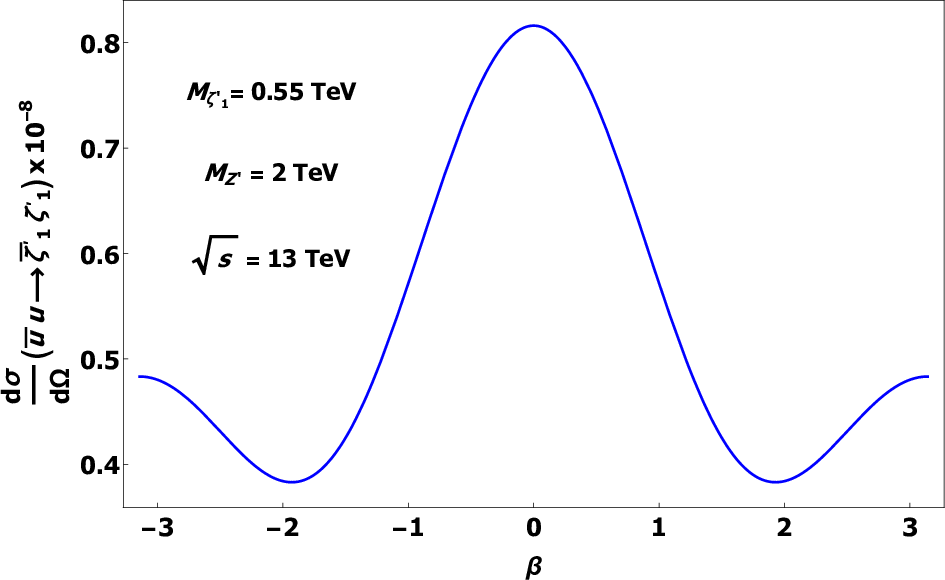
If we fix α=45o\alpha=45^{o}, s=13​TeV\sqrt{s}=13\,\mbox{TeV}, MZ=2​TeVM_{Z}=2\,\mbox{TeV} and Mζ1′=0.5​TeVM_{\zeta^{\prime}_{1}}=0.5\,\mbox{TeV}, the result (4.17) appears as a function of β\beta. This differential cross section in terms of the β\beta-angle is plotted in the figure (6).

Refer to caption
Figure 6: The differential cross section of u¯​u→ζ¯1′​ζ1′\bar{u}\,u\rightarrow\bar{\zeta}^{\prime}_{1}\,\zeta^{\prime}_{1} as function of the β\beta-angle. We use here the values for masses Mζ1′=0.5​TeVM_{\zeta^{\prime}_{1}}=0.5\,\mbox{TeV} and MZ′=2​TeVM_{Z^{\prime}}=2\,\mbox{TeV}, the CM-energy as s=13​TeV\sqrt{s}=13\,\mbox{TeV}, with a mixing angle of α=45o\alpha=45^{o}.

Returning to the expression (4.17), the total cross section as a function of the α\alpha-mixing angle is given by

σ⁡(u¯​u→ζ¯1′​ζ1′)\displaystyle\sigma(\bar{u}\,u\,\rightarrow\,\bar{\zeta}^{\prime}_{1}\,\zeta^{\prime}_{1}) =\displaystyle= π​αe24​s1cos4⁡θW​sin4⁡(2​α)(1−MZ′2s)−2×\displaystyle\frac{\pi\,\alpha_{e}^{2}}{4s}\frac{1}{\cos^{4}\theta_{W}\sin^{4}(2\alpha)}\left(1-\frac{M_{Z^{\prime}}^{2}}{s}\right)^{\!\!-2}\times (4.18)
×[43​cos4⁡α⁡(1−4​Mζi′2s)+(1−53​sin2⁡α)2],\displaystyle\hskip-14.22636pt\times\left[\frac{4}{3}\cos^{4}\alpha\left(1-\frac{4M_{\zeta^{\prime}_{i}}^{2}}{s}\right)+\left(1-\frac{5}{3}\sin^{2}\alpha\right)^{2}\right]\;,

in which the σ\sigma-function is illustrated in the figure (7).

Refer to caption
Figure 7: The total cross section of u¯​u→ζ¯1′​ζ1′\bar{u}\,u\,\rightarrow\,\bar{\zeta}^{\prime}_{1}\,\zeta^{\prime}_{1} as function of the Z′Z^{\prime}-mass. Here, we adopt the CM-energy values by s=13​TeV\sqrt{s}=13\,\mbox{TeV} and s=8​TeV\sqrt{s}=8\,\mbox{TeV}.

When α=45o\alpha=45^{o}, the total cross section assumes the value

σ⁡(u¯​u→ζ¯1′​ζ1′)≃3.76×10⁻⁷​TeV−2.\displaystyle\sigma(\bar{u}\,u\,\rightarrow\,\bar{\zeta}^{\prime}_{1}\,\zeta^{\prime}_{1})\simeq 3.76\times 10^{-7}\,\,\mbox{TeV}^{-2}\;. (4.19)

5 The MDM for the ζi\zeta_{i}-fermions

In this Section, we investigate the magnetic properties of ζi\zeta_{i}-fermions through it Magnetic Dipole Momentum (MDM) The mixing of ζi\zeta_{i} with the right-neutrino components motivates us to understand if the ζi\zeta_{i}-MDM depends on its mass, as it happens in the case of neutrinos. For a review on the neutrinos’ MDMs, go to the references [29, 30, 32, 31, 33]. We start off with the field equations in the mixed basis to obtain the so-called Transition Dipole Momenta (TDM). The Dirac equations for the νi\nu_{i}-neutrinos and ζi\zeta_{i}-fermions from (3.1) in the momentum space are given by

(/p−mνi)uνi(p)−Mi​jR​Luζj(p)\displaystyle\left(\,/\penalty{\!\!\!p}-m_{\nu_{i}}\,\right)u_{\nu_{i}}(p)-M_{ij}^{RL}\,u_{\zeta_{j}}(p) =\displaystyle= 0\displaystyle 0
(/p−mζi)uζi(p)−Mi​jL​Ruνj(p)\displaystyle\left(\,/\penalty{\!\!\!p}-m_{\zeta_{i}}\,\right)u_{\zeta_{i}}(p)-M_{ij}^{LR}\,u_{\nu_{j}}(p) =\displaystyle= 0,\displaystyle 0\;, (5.1)

where mνim_{\nu_{i}} and mζim_{\zeta_{i}} are the masses if we make the mixed coupling constants Yi​j=Zi​j→ 0Y_{ij}=Z_{ij}\,\rightarrow\,0. The functions uνi​(p)u_{\nu_{i}}(p) and uζi​(p)u_{\zeta_{i}}(p) are the wave plane amplitudes of νi\nu_{i} and ζi\zeta_{i} in the mixed basis, respectively. For simplicity, we have defined the matrices MR​LM_{RL} and ML​RM_{LR} as combination of Left- and Right-components :

Mi​jR​L\displaystyle M_{ij}^{RL} :⁣=\displaystyle:= Yi​j​v​R+Zi​j​u​L2,\displaystyle\frac{Y_{ij}\,v\,R+Z_{ij}\,u\,L}{\sqrt{2}}\;,
Mi​jL​R\displaystyle M_{ij}^{LR} :⁣=\displaystyle:= Yi​j​v​L+Zi​j​u​R2.\displaystyle\frac{Y_{ij}\,v\,L+Z_{ij}\,u\,R}{\sqrt{2}}\;. (5.2)

The hermitian conjugate of (5.1) is written below:

u¯νi(p)(/p−mνi)−u¯ζj(p)Mi​jLR†\displaystyle\bar{u}_{\nu_{i}}(p)\left(\,/\penalty{\!\!\!p}-m_{\nu_{i}}\,\right)-\bar{u}_{\zeta_{j}}(p)\,M_{ij}^{LR\,\dagger} =\displaystyle= 0\displaystyle 0
u¯ζi(p)(/p−mζi)−u¯νj(p)Mi​jRL†\displaystyle\bar{u}_{\zeta_{i}}(p)\left(\,/\penalty{\!\!\!p}-m_{\zeta_{i}}\,\right)-\bar{u}_{\nu_{j}}(p)\,M_{ij}^{RL\,\dagger} =\displaystyle= 0.\displaystyle 0\;. (5.3)

If we substitute pμp^{\mu} by p′μp^{\prime\mu} in (5.3), we can combine the hermitian conjugate equations with the equations (5.1) to obtain the following tree-level Gordon decompositions:

u¯νi​(p′)​γμ​uνi​(p)=u¯νi​(p′)​(ℓμ2​mνi+i​σμ​ν​qν2​mνi)​uνi​(p)\displaystyle\bar{u}_{\nu_{i}}(p^{\prime})\,\gamma^{\mu}\,u_{\nu_{i}}(p)=\bar{u}_{\nu_{i}}(p^{\prime})\!\left(\frac{\ell^{\mu}}{2m_{\nu_{i}}}+i\,\frac{\sigma^{\mu\nu}q_{\nu}}{2m_{\nu_{i}}}\right)\!u_{\nu_{i}}(p)
−u¯νi(p′)(μi​jℓμ2​mνi+μi​jiσμ​ν​qν2​mνi+ηi​jqμ​γ52​mνi+ηi​jiσμ​ν​ℓν2​mνiγ5)uζj(p)+h. c.,\displaystyle-\bar{u}_{\nu_{i}}(p^{\prime})\!\left(\hskip-7.11317pt\phantom{\frac{1}{2}}\,\mu_{ij}\,\frac{\ell^{\mu}}{2m_{\nu_{i}}}+\mu_{ij}\,i\,\frac{\sigma^{\mu\nu}q_{\nu}}{2m_{\nu_{i}}}+\eta_{ij}\,\frac{q^{\mu}\gamma_{5}}{2m_{\nu_{i}}}+\eta_{ij}\,i\,\frac{\sigma^{\mu\nu}\ell_{\nu}}{2m_{\nu_{i}}}\,\gamma^{5}\hskip-7.11317pt\phantom{\frac{1}{2}}\,\right)u_{\zeta_{j}}(p)+\mbox{h. c.}\,, (5.4)

and

u¯ζi​(p′)​γμ​uζi​(p)=u¯ζi​(p′)​(ℓμ2​mζi+i​σμ​ν​qν2​mζi)​uζi​(p)\displaystyle\bar{u}_{\zeta_{i}}(p^{\prime})\,\gamma^{\mu}\,u_{\zeta_{i}}(p)=\bar{u}_{\zeta_{i}}(p^{\prime})\left(\frac{\ell^{\mu}}{2m_{\zeta_{i}}}+i\,\frac{\sigma^{\mu\nu}q_{\nu}}{2m_{\zeta_{i}}}\right)u_{\zeta_{i}}(p)
−u¯ζi(p′)(μi​jℓμ2​mζi+μi​jiσμ​ν​qν2​mζi+ηi​jqμ​γ52​mζi+ηi​jiσμ​ν​ℓν2​mζiγ5)uνj(p)+h. c.,\displaystyle-\bar{u}_{\zeta_{i}}(p^{\prime})\!\left(\hskip-7.11317pt\phantom{\frac{1}{2}}\,\mu_{ij}\,\frac{\ell^{\mu}}{2m_{\zeta_{i}}}+\mu_{ij}\,i\,\frac{\sigma^{\mu\nu}q_{\nu}}{2m_{\zeta_{i}}}+\eta_{ij}\,\frac{q^{\mu}\gamma_{5}}{2m_{\zeta_{i}}}+\eta_{ij}\,i\,\frac{\sigma^{\mu\nu}\ell_{\nu}}{2m_{\zeta_{i}}}\,\gamma_{5}\phantom{\frac{1}{2}}\hskip-7.11317pt\right)u_{\nu_{j}}(p)+\mbox{h. c.}\;, (5.5)

where qμ=pμ−p′μq^{\mu}=p^{\mu}-p^{\prime\mu} is the photon’s transfer momentum, and ℓμ:=pμ+p′μ\ell^{\mu}:=p^{\mu}+p^{\prime\mu} is the total 44-momentum. These expressions yield the currents of neutrinos with the ζi\zeta_{i}-fermions of the model, written in momentum space, that we refer to as transition terms. The coefficients μi​j\mu_{ij} and ηi​j\eta_{ij} are matrix elements that depend on the Yukawa complex constant coupling and the uu-VEV scale :

μi​j\displaystyle\mu_{ij} =\displaystyle= 12​2​Zi​j​u+Yi​j​vmζi+mνi,\displaystyle\frac{1}{2\sqrt{2}}\,\frac{Z_{ij}\,u+Y_{ij}\,v}{m_{\zeta_{i}}+m_{\nu_{i}}}\;,
ηi​j\displaystyle\eta_{ij} =\displaystyle= 12​2​Zi​j​u−Yi​j​vmζi+mνi.\displaystyle\frac{1}{2\sqrt{2}}\,\frac{Z_{ij}\,u-Y_{ij}\,v}{m_{\zeta_{i}}+m_{\nu_{i}}}\;. (5.6)

Here, if we use that mζi≫mνim_{\zeta_{i}}\gg m_{\nu_{i}}, and u≫vu\gg v, so we can approximate Yi​j​v+Zi​j​u≈Zi​j​uY_{ij}\,v+Z_{ij}\,u\approx Z_{ij}\,u, and the coefficients μi​j\mu_{ij} and ηi​j\eta_{ij} are approximately equals, μi​j≃ηi​j\mu_{ij}\simeq\eta_{ij}. We also neglect terms of order Zi​j2≈0Z_{ij}^{2}\approx 0 in relation to the linear terms of Zi​jZ_{ij} in (5.4) and (5.5). We observe the emergence of TMDM for neutrinos and ζi\zeta_{i}-fermions in both expressions (5.4) and (5.5). If we multiply these currents by e​Aμe\,A_{\mu}, and using the representation qν→i∂νq_{\nu}\rightarrow i\,\partial_{\nu} for the photon momentum, the terms σμ​ν​qν\sigma^{\mu\nu}q_{\nu} have the following TMDM for the νi\nu_{i}-neutrino :

μi​j(νi)\displaystyle\mu_{ij}^{\,(\nu_{i})} =\displaystyle= e​μi​j2​mνi=e​Zi​j​u4​2​mνi​mζi≃Zi​j4​2​(2.8​TeVmζi)​(1​MeVmνi)​μB.\displaystyle\frac{e\,\mu_{ij}}{2\,m_{\nu_{i}}}=\frac{e\,Z_{ij}\,u}{4\sqrt{2}\,m_{\nu_{i}}\,m_{\zeta_{i}}}\simeq\frac{Z_{ij}}{4\sqrt{2}}\,\left(\frac{2.8\,\mbox{TeV}}{m_{\zeta_{i}}}\right)\,\left(\frac{1\,\mbox{MeV}}{m_{\nu_{i}}}\right)\,\mu_{B}\;. (5.7)

We have a result at tree-level for Dirac neutrinos that depends on the νi\nu_{i}-neutrino mass and the ζi\zeta_{i}-mass. This result allows us to fix an small estimate for the Zi​jZ_{ij} coupling constant using the known result |μ(ν)|≲ 8× 10−15​μB|\mu^{(\nu)}|\,\lesssim\,8\,\times\,10^{-15}\,\mu_{B} in the literature [29]. We consider the mass spectrum of mνi∼ 1​eVm_{\nu_{i}}\,\sim\,1\,\mbox{eV} for neutrinos, the mass of mζ1=0.5​TeVm_{\zeta_{1}}=0.5\,\mbox{TeV} for ζ1\zeta_{1}-fermion, and u=2.8​TeVu=2.8\,\mbox{TeV}. In so doing, the expression (5.7) yields the Zi​jZ_{ij} coupling constant below :

|Zi​j|≲ 7.5× 10−21.\displaystyle|Z_{ij}|\,\lesssim\,7.5\,\times\,10^{-21}\;. (5.8)

The TMDM for ζi\zeta_{i}-hidden fermion is given by expression

μi​j(ζi)=e​μi​j2​mζi=Zi​j4​2​(2.8​TeVmζi)​(1​MeVmζi)​μB.\displaystyle\mu_{ij}^{\,(\zeta_{i})}=\frac{e\,\mu_{ij}}{2\,m_{\zeta_{i}}}=\frac{Z_{ij}}{4\sqrt{2}}\,\left(\frac{2.8\,\mbox{TeV}}{m_{\zeta_{i}}}\right)\,\left(\frac{1\,\mbox{MeV}}{m_{\zeta_{i}}}\right)\,\mu_{B}\;. (5.9)

Therefore, we can estimate the TMDM for the ζ1\zeta_{1}-hidden fermion :

|μi​j(ζ1)|≲ 1.6× 10−26​μB,\displaystyle|\mu_{ij}^{\,(\zeta_{1})}|\,\lesssim\,1.6\,\times\,10^{-26}\,\mu_{B}\;, (5.10)

where μB=3×10⁻⁷​eV−1\mu_{B}=3\times 10^{-7}\,\mbox{eV}^{-1} is the Bohr magneton, in natural units c=ℏ=1c=\hbar=1.

The important contribution for the MDM of ζi\zeta_{i} combines two external lines of ζi′\zeta^{\prime}_{i} with one external line of photon in a one-loop diagram. This possible loop diagram emerges when we work in the mass basis ζi′\zeta^{\prime}_{i} due to the vertex W±−ζ′−ℓ′W^{\pm}-\zeta^{\prime}-\ell^{\prime}. This vertex depends on the θ\theta-mixing angle, and we belief that it must be a small effect. Obviously, the vertex goes to zero, when θ→ 0\theta\,\rightarrow\,0. The vertex at one loop is illustrated in the figure (8).

0,0.5)(8.8,5) pscoil[coilaspect=0,coilarm=0.1,coilwidth=0.25,coilheight=1.3,linecolor=black](2,1)(5,1) pscoil[coilaspect=0,coilarm=0,coilwidth=0.25,coilheight=1.3,linecolor=black](3.5,2.5)(3.5,4) W ¯ ζ ′ ζ ′ ℓ ¯ ℓ γ = q - p p ′ p ′ + k p + k p ′ p k

Figure 8: The first contribution at one-loop for the MDM of ζi′\zeta^{\prime}_{i}-fermion combining the W±−ζ′−ℓ′W^{\pm}-\zeta^{\prime}-\ell^{\prime} vertex with the external photon.

0,0.5)(8.8,5) pscoil[coilaspect=0,coilarm=0.1,coilwidth=0.25,coilheight=1.3,linecolor=black](2,1)(3.5,2.5) pscoil[coilaspect=0,coilarm=0.1,coilwidth=0.25,coilheight=1.3,linecolor=black](3.5,2.5)(5,1) pscoil[coilaspect=0,coilarm=0,coilwidth=0.25,coilheight=1.3,linecolor=black](3.5,2.5)(3.5,4) ℓ ¯ ζ ′ ζ ′ W - W + γ = q - p p ′ p ′ + k p + k p ′ p k

Figure 9: The second contribution at one-loop for the MDM of theζi′\zeta^{\prime}_{i}-fermion with the W+​W−W^{+}W^{-}-photon vertex of the GSW model.

Following the previous rules, the one-loop vertex (8) is represented by the integral

Λ(1)​i​jμ​(p,p′)\displaystyle\Lambda_{(1)ij}^{\mu}(p,p^{\prime}) =\displaystyle= −g2​θ28Vi​kVk​j∫d4​k(2​π)4γα(1−γ5)i(/k+/p′+m)(k+p′)2−m2×\displaystyle-\frac{g^{2}\theta^{2}}{8}\,V_{ik}V_{kj}\int\frac{d^{4}k}{(2\pi)^{4}}\,\gamma^{\alpha}\left(1-\gamma_{5}\right)\frac{i\left(/\penalty{\!\!\!k}+/\penalty{\!\!\!p}^{\prime}+m\right)}{(k+p^{\prime})^{2}-m^{2}}\,\times (5.11)
×(i​e​γμ)​i(/k+/p+m)(k+p)2−m2​γα​(1−γ5)​−ik2−mW2.\displaystyle\times\,\left(ie\gamma^{\mu}\right)\,\frac{i\left(/\penalty{\!\!\!k}+/\penalty{\!\!\!p}+m\right)}{(k+p)^{2}-m^{2}}\,\gamma_{\alpha}\left(1-\gamma_{5}\right)\frac{-i}{k^{2}-m_{W}^{2}}\;.

The second contribution comes from the combination of W±−ζ′−ℓ′W^{\pm}-\zeta^{\prime}-\ell^{\prime} interaction with the vertex W±W^{\pm}-photon of the GSW model. It is illustrated in the figure (9). The Feynman rules yield the momentum space loop integral below

Λ(2)​i​jμ(p,p′)=−g2​θ28Vi​kVk​j∫d4​k(2​π)4γα(1−γ5)−i(k+p′)2−mW2×\displaystyle\Lambda_{(2)ij}^{\mu}(p,p^{\prime})=-\frac{g^{2}\theta^{2}}{8}\,V_{ik}V_{kj}\int\frac{d^{4}k}{(2\pi)^{4}}\,\gamma_{\alpha}\left(1-\gamma_{5}\right)\,\frac{-i}{\left(k+p^{\prime}\right)^{2}-m_{W}^{2}}\,\times
×Vμ​α​β​(q,k+p′,−k−p)​−i(k+p)2−mW2​i(/k+m)k2−m2​γβ​(1−γ5).\displaystyle\times\,V^{\mu\alpha\beta}\left(q,k+p^{\prime},-k-p\right)\frac{-i}{\left(k+p\right)^{2}-m_{W}^{2}}\,\frac{i\left(/\penalty{\!\!\!k}+m\right)}{k^{2}-m^{2}}\,\gamma_{\beta}\left(1-\gamma_{5}\right)\;. (5.12)

We have used the W±W^{\pm}-propagator in the Feynman gauge in the expressions (5.11) and (5.12)(\ref{IntGamma}), Vμ​α​βV^{\mu\alpha\beta} sets the W±−γW^{\pm}-\gamma vertex following the GSW model rules. Well-known techniques to deal with Feynman integrals are introduced to calculate the finite part of these integrals and, then, the contributions for the MDM of ζi\zeta_{i}-fermions. The sum of these two contributions is denoted by Γμ=Λ(1)μ+Λ(2)μ\Gamma^{\mu}=\Lambda_{(1)}^{\mu}+\Lambda_{(2)}^{\mu}, so the finite part of Γμ\Gamma^{\mu} at one-loop is written into the form

Jζi′​(e​m)μ=u¯ζi′​Γi​jμ​uζj′=u¯ζi′​(p′)​[f1​(q2)​γμ+f2​(q2)​γ5​γμ+f3​(q2)​i​σμ​ν​qν+f4​(q2)​qμ​γ5]i​j​uζj′​(p),J_{\zeta^{\prime}_{i}(em)}^{\;\mu}=\bar{u}_{\zeta^{\prime}_{i}}\,\Gamma_{ij}^{\,\mu}\,u_{\zeta^{\prime}_{j}}=\bar{u}_{\zeta^{\prime}_{i}}(p^{\prime})\left[\phantom{\frac{1}{2}}\hskip-7.11317ptf_{1}(q^{2})\,\gamma^{\mu}+f_{2}(q^{2})\gamma_{5}\,\gamma^{\mu}+f_{3}(q^{2})\,i\,\sigma^{\mu\nu}q_{\nu}+f_{4}(q^{2})\,q^{\mu}\gamma_{5}\,\right]_{ij}\!\!u_{\zeta^{\prime}_{j}}(p)\;, (5.13)

where f1f_{1}, f2f_{2}, f3f_{3} and f4f_{4} are the form factors of the previous diagrams in this order. The current conservation implies that qμ​Jζi′​(e​m)μ=0q_{\mu}J_{\zeta^{\prime}_{i}(em)}^{\mu}=0, then under this condition we obtain the relation f2(q2)=−q2f4(q2)/2Mζi′f_{2}(q^{2})=-q^{2}\,f_{4}(q^{2})/2M_{\zeta^{\prime}_{i}}. Thereby, the EM-current of ζi′\zeta^{\prime}_{i} is reduced to expression

Jζi′​(e​m)μ=u¯ζi′​Γi​jμ​uζj′=u¯ζi′​(p′)​[f1​(q2)​γμ+fA​(q2)​γ5​(qμ/q−q2​γμ)+f3​(q2)​i​σμ​ν​qν]i​j​uζj′​(p).J_{\zeta^{\prime}_{i}(em)}^{\;\mu}=\bar{u}_{\zeta^{\prime}_{i}}\,\Gamma_{ij}^{\,\mu}\,u_{\zeta^{\prime}_{j}}=\bar{u}_{\zeta^{\prime}_{i}}(p^{\prime})\left[\phantom{\frac{1}{2}}\hskip-7.11317ptf_{1}(q^{2})\,\gamma^{\mu}+f_{A}(q^{2})\gamma_{5}\left(q^{\mu}\,/\penalty{\!\!\!q}-q^{2}\,\gamma^{\mu}\right)+f_{3}(q^{2})\,i\,\sigma^{\mu\nu}q_{\nu}\,\right]_{ij}\!\!u_{\zeta^{\prime}_{j}}(p)\;. (5.14)

We have also used here the mass on-shell conditions for ζi′\zeta^{\prime}_{i}-fermions : /p​uζi′​(p)=Mζi′​uζi′​(p)/\penalty{\!\!\!p}\,u_{\zeta^{\prime}_{i}}(p)=M_{\zeta^{\prime}_{i}}\,u_{\zeta^{\prime}_{i}}(p), u¯ζi′​(p′)/p′=u¯ζi′​(p′)​Mζi′\bar{u}_{\zeta^{\prime}_{i}}(p^{\prime})\,/\penalty{\!\!\!p}^{\prime}=\bar{u}_{\zeta^{\prime}_{i}}(p^{\prime})\,M_{\zeta^{\prime}_{i}} and p2=p′2=Mζi′2p^{2}=p^{\prime 2}=M_{\zeta^{\prime}_{i}}^{2}. The amplitudes u¯ζi′​(p′)\bar{u}_{\zeta^{\prime}_{i}}(p^{\prime}) and uζi′​(p)u_{\zeta^{\prime}_{i}}(p) stand for the plane wave solutions in the diagonal basis of ζi′\zeta^{\prime}_{i}-fermions. The f1f_{1}-form factor is the contribution to electric charge given by

f1(q2)i​j=e​g2​θ232​π2Vi​kVk​j∫01dxdydzδ(x+y+z−1)×\displaystyle f_{1}(q^{2})_{ij}=\frac{eg^{2}\theta^{2}}{32\pi^{2}}\,V_{ik}V_{kj}\int_{0}^{1}dx\,dy\,dz\,\delta(x+y+z-1)\,\times
×[Mζi′2​z​(4−z)−m2Mζi′2​z​(1−z)−mW2​z−m2​z​(1−z)+q2​x​y\displaystyle\times\,\left[\,\frac{M_{\zeta_{i}^{\prime}}^{2}\,z(4-z)-m^{2}}{M_{\zeta^{\prime}_{i}}^{2}\,z(1-z)-m_{W}^{2}z-m^{2}\,z(1-z)+q^{2}xy}\right.
−Mζi′2​(1−z)​(2+3​z)Mζi′2​z​(1−z)−mW2​(1−z)−m2​z+q2​x​y].\displaystyle\left.-\frac{M_{\zeta_{i}^{\prime}}^{2}\,(1-z)(2+3z)}{M_{\zeta^{\prime}_{i}}^{2}\,z(1-z)-m_{W}^{2}(1-z)-m^{2}z+q^{2}xy}\,\right]\,. (5.15)

The second term in (5.14) is known as the anapole (or toroidal momentum) term with the fAf_{A}-form factor that follows:

fA(q2)i​j=f4​(q2)i​j2​Mζi′=e​g2​θ232​π2Vi​kVk​j∫01dxdydzδ(x+y+z−1)×\displaystyle f_{A}(q^{2})_{ij}=\frac{f_{4}(q^{2})_{ij}}{2M_{\zeta^{\prime}_{i}}}=\frac{eg^{2}\theta^{2}}{32\pi^{2}}\,V_{ik}V_{kj}\int_{0}^{1}dx\,dy\,dz\,\delta(x+y+z-1)\,\times
×[2+2​z−2​(x−y)2Mζi′2​z​(1−z)−mW2​z−m2​z​(1−z)+q2​x​y\displaystyle\times\,\left[\,\frac{2+2z-2(x-y)^{2}}{M_{\zeta^{\prime}_{i}}^{2}\,z(1-z)-m_{W}^{2}z-m^{2}\,z(1-z)+q^{2}xy}\right.
−3​(1−z)−2​(x−y)2Mζi′2​z​(1−z)−mW2​(1−z)−m2​z+q2​x​y].\displaystyle\left.-\frac{3(1-z)-2(x-y)^{2}}{M_{\zeta^{\prime}_{i}}^{2}\,z(1-z)-m_{W}^{2}(1-z)-m^{2}z+q^{2}xy}\,\right]\,. (5.16)

The f3f_{3}-form factor is the contribution to the ζi′\zeta^{\prime}_{i}-fermion MDM :

f3(q2)i​j=−e​g2​θ232​π2Mζi′Vi​kVk​j∫01dxdydzδ(x+y+z−1)×\displaystyle f_{3}(q^{2})_{ij}=-\frac{eg^{2}\theta^{2}}{32\pi^{2}}\,M_{\zeta^{\prime}_{i}}\,V_{ik}V_{kj}\int_{0}^{1}dx\,dy\,dz\,\delta(x+y+z-1)\times
×[z⁡(1−z)Mζi′2​z​(1−z)−mW2​z−m2​z​(1−z)+q2​x​y\displaystyle\times\left[\,\frac{z(1-z)}{M_{\zeta^{\prime}_{i}}^{2}\,z(1-z)-m_{W}^{2}z-m^{2}z(1-z)+q^{2}xy}\right.
−(1−z)​(1/2−z)Mζi′2​z​(1−z)−mW2​(1−z)−m2​z+q2​x​y].\displaystyle\left.-\frac{(1-z)(1/2-z)}{M_{\zeta^{\prime}_{i}}^{2}\,z(1-z)-m_{W}^{2}(1-z)-m^{2}z+q^{2}xy}\,\right]\,.\hskip 14.22636pt (5.17)

The on-shell condition for the external photon imposes q2=0q^{2}=0. Therefore, all the form factors depend on the masses of ζi′\zeta^{\prime}_{i}-fermion, W±W^{\pm} and the lepton mass, where we take Mζi′,mW≫mM_{\zeta^{\prime}_{i}}\,,\,m_{W}\gg m and also consider Mζi′>mWM_{\zeta^{\prime}_{i}}>m_{W} . Under these conditions, the elements of the f1f_{1}-factor are

f1​(0)i​j=−e​g2​θ216​π2​Vi​k​Vk​j​(1+mW2Mζi′2)​[2−(1−mW2Mζi′2)​ln⁡(Mζi′2mW2−1)].\displaystyle f_{1}(0)_{ij}=-\frac{eg^{2}\theta^{2}}{16\pi^{2}}\,V_{ik}V_{kj}\,\left(1+\frac{m_{W}^{2}}{M_{\zeta^{\prime}_{i}}^{2}}\right)\left[2-\left(1-\frac{m_{W}^{2}}{M_{\zeta^{\prime}_{i}}^{2}}\right)\ln\left(\frac{M_{\zeta^{\prime}_{i}}^{2}}{m_{W}^{2}}-1\right)\right]\;. (5.18)

The interaction of AμA^{\mu}-field with the ζi′\zeta^{\prime}_{i}-current yields the form factor in the limit q2→ 0q^{2}\,\rightarrow\,0

u¯ζi′(p′)Γi​jμ(q)uζj′(p)Aμ=q2→0−f3(0)i​ju¯ζi′(p′)σ→⋅𝐁→uζj′(p),\bar{u}_{\zeta^{\prime}_{i}}(p^{\prime})\,\Gamma_{ij}^{\mu}(q)\,u_{\zeta^{\prime}_{j}}(p)\,A_{\mu}\!\stackrel{{\scriptstyle q^{2}\rightarrow 0}}{{=}}-f_{3}(0)_{ij}\,\bar{u}_{\zeta^{\prime}_{i}}(p^{\prime})\,\vec{\sigma}\cdot\vec{{\bf B}}\,u_{\zeta^{\prime}_{j}}(p)\;, (5.19)

where the transfer momentum is represented in an operator form, qν→i∂νq_{\nu}\rightarrow i\,\partial_{\nu}. We have considered the EM tensor as Fμ​ν=(0,ϵi​j​k​Bk)F^{\mu\nu}=\left(0,\epsilon^{ijk}B^{k}\right) with an external magnetic field, and σi​j=εi​j​k​σk\sigma^{ij}=\varepsilon^{ijk}\sigma^{k}. We identify the elements of ζi′\zeta^{\prime}_{i}-MDM as μM​i​j(ζi′)=f3​(0)i​j\mu_{M\,ij}^{\,(\zeta^{\prime}_{i})}=f_{3}(0)_{ij}, thus, the form factor f3​(0)i​jf_{3}(0)_{ij} can be written in terms of electron’s mass and the Bohr magneton :

μM​i​j(ζi′)=−3​GF​me​Mζi′4​2​π2​θ2​Vi​k​Vk​j​mW2Mζi′2​[1−13​ln⁡(Mζi′2mW2−1)+mW2Mζi′2]​μB.\displaystyle\mu_{M\,ij}^{\,(\zeta^{\prime}_{i})}=-\frac{3G_{F}m_{e}M_{\zeta^{\prime}_{i}}}{4\sqrt{2}\pi^{2}}\,\theta^{2}\,V_{ik}V_{kj}\,\frac{m_{W}^{2}}{M_{\zeta^{\prime}_{i}}^{2}}\left[1-\frac{1}{3}\ln\left(\frac{M_{\zeta^{\prime}_{i}}^{2}}{m_{W}^{2}}-1\right)+\frac{m_{W}^{2}}{M_{\zeta^{\prime}_{i}}^{2}}\right]\,\mu_{B}\,. (5.20)

This depends on the Mζi′M_{\zeta^{\prime}_{i}}-mass and on the ratio mW/Mζi′m_{W}/M_{\zeta^{\prime}_{i}}, if we use mW=80​GeVm_{W}=80\,\mbox{GeV} and Mζ1′=0.5​TeVM_{\zeta^{\prime}_{1}}=0.5\,\mbox{TeV}, we have mW/Mζ1′≃0.14m_{W}/M_{\zeta^{\prime}_{1}}\simeq 0.14, and θ≃−9× 10−8\theta\simeq-9\,\times\,10^{-8}. With these values, the MDM for the ζ1′\zeta^{\prime}_{1}-hidden fermion gets the one-loop contribution

μM​i​j(ζ1′)≃1.2× 10−21​Vi​k​Vk​j​μB.\displaystyle\mu_{M\,ij}^{\,(\zeta^{\prime}_{1})}\simeq 1.2\,\times\,10^{-21}\;V_{ik}V_{kj}\,\mu_{B}\;. (5.21)

Therefore, the elements i​jij of ζ1′\zeta^{\prime}_{1}-MDM depend on the VV-matrix elements as given in (3.29). For example, for the diagonal elements, μM​i​i(ζ1′)≃1.2× 10−21​Vi​k​Vk​i​μB\mu_{M\,ii}^{\,(\zeta^{\prime}_{1})}\simeq 1.2\,\times\,10^{-21}\;V_{ik}V_{ki}\,\mu_{B} with the implicit sum runs on the kk-index. For i=1i=1, the element μM​ 11(ζ1′)\mu_{M\,11}^{\,(\zeta^{\prime}_{1})} depends on the cosines of mixing angles θ12\theta_{12} and θ13\theta_{13}, so we obtain the upper bound

μM​ 11(ζ1′)≃1.2× 10−21​c12 2​c13 2​μB≲1.2× 10−21​μB.\displaystyle\mu_{M\,11}^{\,(\zeta^{\prime}_{1})}\simeq 1.2\,\times\,10^{-21}\,c_{12}^{\,2}\,c_{13}^{\,2}\;\mu_{B}\lesssim 1.2\,\times\,10^{-21}\,\mu_{B}\;. (5.22)

6 The X-boson scenario at the MeV-scale and below

Contrary to Section II, the XX-boson scenario is introduced through the SSB pattern-II mechanism in which the new VEV-scale is at a lower scale with respect to the EW model, u≪v=246​GeVu\ll v=246\,\mbox{GeV}. This SSB pattern-II can be followed in more details in [28]; the original S​UL​(2)×UR​(1)J×U​(1)KSU_{L}(2)\times U_{R}(1)_{J}\times U(1)_{K}-symmetry is broken as below :

S​UL​(2)×UR​(1)J×U​(1)K⟼⟨Φ⟩0U​(1)G×U​(1)K⟼⟨Ξ⟩0U​(1)e​m,SU_{L}(2)\times U_{R}(1)_{J}\times U(1)_{K}\stackrel{{\scriptstyle\langle\Phi\rangle_{0}}}{{\longmapsto}}U(1)_{G}\times U(1)_{K}\stackrel{{\scriptstyle\langle\Xi\rangle_{0}}}{{\longmapsto}}U(1)_{em}\;, (6.1)

where we have the VEV scale-uu that defines a lightest massive boson, that can describe the physics of the dark-photon with mass bound of mA′<8​GeVm_{A^{\prime}}<8\,\mbox{GeV} [24], the XX-boson of mass 17​MeV17\,\mbox{MeV}, or also can describe the para-photon physics at the Sub-eV-scale. We call the U​(1)GU(1)_{G}-group as the result from the mixing of S​UL​(2)×UR​(1)JSU_{L}(2)\times U_{R}(1)_{J}. The generator GG of U​(1)GU(1)_{G} is given by G=I3+JG=I^{3}+J. In both cases, the extra-sector U​(1)KU(1)_{K} of CμC^{\mu} couples kinetically with BμB^{\mu} of UR​(1)JU_{R}(1)_{J} by means of mixing parameter χ\chi given by

ℒg​a​u​g​e=−12​tr​(Fμ​ν 2)−14​Bμ​ν 2−14​Cμ​ν 2+χ2​Bμ​ν​Cμ​ν.{\cal L}_{gauge}=-\frac{1}{2}\,\mbox{tr}\left(F_{\mu\nu}^{\;2}\right)-\frac{1}{4}\,B_{\mu\nu}^{\;2}-\frac{1}{4}\,C_{\mu\nu}^{\;2}+\frac{\chi}{2}\,B_{\mu\nu}\,C^{\mu\nu}\;. (6.2)

Its currently estimated value is 10−6<χ<10−310^{-6}<\chi<10^{-3} for models that discuss hidden photons as dark matter [27].

The sector of fermions is given by the Lagrangian (2.1), but the covariant derivatives must exhibit the millicharged coupling of extra boson CμC^{\mu} of U​(1)KU(1)_{K} with the fermions of the Standard Model. Thus, we modify these couplings introducing the parameters εΨ\varepsilon_{\Psi} and εζ\varepsilon_{\zeta}

Dμ​ΨL\displaystyle\!\!\!\!\!\!D_{\mu}\Psi_{L} =\displaystyle= (∂μ+igAμaσa2+iJLg′Bμ+iKLεΨg′′Cμ)ΨL,\displaystyle\left(\partial_{\mu}+i\,g\,A_{\mu}^{\,a}\frac{\sigma^{a}}{2}+i\,J_{L}\,g^{\prime}\,B_{\mu}+i\,K_{L}\,\varepsilon_{\Psi}\,g^{\prime\prime}\,C_{\mu}\phantom{\frac{1}{2}}\!\!\!\!\!\right)\Psi_{L}\,,
Dμ​ΨR\displaystyle D_{\mu}\Psi_{R} =\displaystyle= (∂μ+iJRg′Bμ+iKRεΨg′′Cμ)ΨR,\displaystyle\left(\phantom{\frac{1}{2}}\!\!\!\!\partial_{\mu}+i\,J_{R}\,g^{\prime}\,B_{\mu}+i\,K_{R}\,\varepsilon_{\Psi}\,g^{\prime\prime}\,C_{\mu}\right)\Psi_{R}\,,
Dμ​νi​R\displaystyle D_{\mu}\nu_{iR} =\displaystyle= (∂μ+iJRg′Bμ+iKRενg′′Cμ)νi​R,\displaystyle\left(\phantom{\frac{1}{2}}\!\!\!\!\partial_{\mu}+i\,J_{R}\,g^{\prime}\,B_{\mu}+i\,K_{R}\,\varepsilon_{\nu}\,g^{\prime\prime}\,C_{\mu}\right)\nu_{iR}\,,
Dμ​ζi\displaystyle D_{\mu}\zeta_{i} =\displaystyle= (∂μ+iJζg′Bμ+iKζεζg′′Cμ)ζi,\displaystyle\left(\phantom{\frac{1}{2}}\!\!\!\!\partial_{\mu}+i\,J_{\zeta}\,g^{\prime}\,B_{\mu}+i\,K_{\zeta}\,\varepsilon_{\zeta}\,g^{\prime\prime}\,C_{\mu}\right)\zeta_{i}\,, (6.3)

that represent the magnitude of the weaker interaction with the XX-boson mentioned in (1.2). Furthermore, the Ξ\Xi-Higgs sector has the modified covariant derivative

DμΞ(x)=(∂μ+iJΞg′Bμ+iKΞεΞg′′Cμ)Ξ(x).\displaystyle D_{\mu}\Xi(x)=\left(\phantom{\frac{1}{2}}\!\!\!\!\partial_{\mu}+i\,J_{\Xi}\,g^{\prime}\,B_{\mu}+i\,K_{\Xi}\,\varepsilon_{\Xi}\,g^{\prime\prime}\,C_{\mu}\right)\Xi(x)\,. (6.4)

The fermion notation is kept like in the previous Z′Z^{\prime}-model, but the particle content is modified to insure an anomaly-free model:

Li\displaystyle L_{i} =\displaystyle= (νeℓe)L,(νμℓμ)L,(ντℓτ)L:(𝟐¯,−12,−12),\displaystyle\left(\begin{array}[]{c}\nu_{e}\\ \ell_{e}\\ \end{array}\right)_{L},\left(\begin{array}[]{c}\nu_{\mu}\\ \ell_{\mu}\\ \end{array}\right)_{L},\left(\begin{array}[]{c}\nu_{\tau}\\ \ell_{\tau}\\ \end{array}\right)_{L}\hskip-2.84544pt:\left(\underline{{\bf 2}},-\frac{1}{2},-\frac{1}{2}\right)\,,
Qi​L\displaystyle Q_{iL} =\displaystyle= (ud)L,(cs)L,(tb)L:(𝟐¯,+16,+16),\displaystyle\left(\begin{array}[]{c}u\\ d\\ \end{array}\right)_{L},\left(\begin{array}[]{c}c\\ s\\ \end{array}\right)_{L},\left(\begin{array}[]{c}t\\ b\\ \end{array}\right)_{L}\hskip-2.84544pt:\left(\underline{{\bf 2}},+\frac{1}{6},+\frac{1}{6}\right)\,,
ℓi​R\displaystyle\ell_{iR} =\displaystyle= {eR,μR,τR}:(𝟏¯,−1,−1),\displaystyle\left\{\,e_{R}\,,\,\mu_{R}\,,\,\tau_{R}\,\right\}:\left(\underline{{\bf 1}},-1,-1\right)\,,
Qi​R\displaystyle Q_{iR} =\displaystyle= {uR,cR,tR}:(𝟏¯,+23,+23),\displaystyle\left\{\,u_{R}\,,\,c_{R}\,,\,t_{R}\,\right\}:\left(\underline{{\bf 1}},+\frac{2}{3},+\frac{2}{3}\right)\,,
qi​R\displaystyle q_{iR} =\displaystyle= {dR,sR,bR}:(𝟏¯,−13,−13),\displaystyle\left\{\,d_{R}\,,\,s_{R}\,,\,b_{R}\,\right\}:\left(\underline{{\bf 1}},-\frac{1}{3},-\frac{1}{3}\right)\,,
νi​R\displaystyle\nu_{iR} =\displaystyle= {νe​R,νμ​R,ντ​R}:(𝟏¯,0,0),\displaystyle\left\{\,\nu_{eR}\,,\,\nu_{\mu R}\,,\,\nu_{\tau R}\,\right\}:\left(\underline{{\bf 1}},0,0\right)\,,
ζi​L\displaystyle\zeta_{iL} =\displaystyle= {ζ1​L,ζ2​L,ζ3​L}:(𝟏¯,0,+32),\displaystyle\left\{\,\zeta_{1L}\,,\,\zeta_{2L}\,,\,\zeta_{3L}\,\right\}:\left(\underline{{\bf 1}},0,+\frac{3}{2}\right)\,,
ζi​R\displaystyle\zeta_{iR} =\displaystyle= {ζ1​R,ζ2​R,ζ3​R}:(𝟏¯,0,−32).\displaystyle\left\{\,\zeta_{1R}\,,\,\zeta_{2R}\,,\,\zeta_{3R}\,\right\}:\left(\underline{{\bf 1}},0,-\frac{3}{2}\right)\,. (6.19)

After the SSBs, the free Lagrangian for the neutral gauge fields reads as follows :

ℒg​a​u​g​e=−14​Fμ​ν 2−14​Z~~μ​ν 2−14​X~~μ​ν 2−χW2​Z~~μ​ν​X~~μ​ν+12​mZ~~ 2​Z~~μ 2+12​mX~~ 2​X~~μ 2,\displaystyle{\cal L}_{gauge}=-\frac{1}{4}\,F_{\mu\nu}^{\,2}-\frac{1}{4}\,\tilde{\tilde{Z}}_{\mu\nu}^{\,2}-\frac{1}{4}\,\tilde{\tilde{X}}_{\mu\nu}^{\,2}-\frac{\chi_{W}}{2}\,\tilde{\tilde{Z}}_{\mu\nu}\tilde{\tilde{X}}^{\mu\nu}+\frac{1}{2}\,m_{\tilde{\tilde{Z}}}^{\,2}\,\tilde{\tilde{Z}}_{\mu}^{\,2}+\frac{1}{2}\,m_{\tilde{\tilde{X}}}^{\,2}\,\tilde{\tilde{X}}_{\mu}^{\,2}\;,\hskip 11.38092pt (6.20)

where we have defined

χW:=χsinθW1−χ2​cos2⁡θW,\displaystyle\chi_{W}:=\frac{\chi\,\sin\theta_{W}}{\sqrt{1-\chi^{2}\cos^{2}\theta_{W}}}\;, (6.21)

and the masses of Z~~μ\tilde{\tilde{Z}}^{\mu} and X~~μ\tilde{\tilde{X}}^{\mu} are given by

mZ~~=e​vsin⁡2​θWandmX~~=3​|εΞ|​e​u.\displaystyle m_{\tilde{\tilde{Z}}}=\frac{e\,v}{\sin 2\theta_{W}}\hskip 11.38092pt\mbox{and}\hskip 11.38092ptm_{\tilde{\tilde{X}}}=3\,|\varepsilon_{\Xi}|\,e\,u\;. (6.22)

For more details on the diagonalization procedure, see [28]. The sector of neutral gauge bosons is composed by two Proca fields with the mixing parameter χW\chi_{W} in the kinetic term.

Here, the Weinberg mixing angle θW\theta_{W} satisfies the parametrization

e=g′′=gsinθW=g′cosθW.\displaystyle e=g^{\prime\prime}=g\,\sin\theta_{W}=g^{\prime}\,\cos\theta_{W}\;. (6.23)

In the gauge sector, Z~~μ\tilde{\tilde{Z}}^{\mu} acquires a mass due to VEV-scale of v=246​GeVv=246\,\mbox{GeV}, and X~~μ\tilde{\tilde{X}}^{\mu} mass is due to lower VEV-scale uu. For convenience, we use here the notation Z~~μ\tilde{\tilde{Z}}^{\mu} and X~~μ\tilde{\tilde{X}}^{\mu} because they are not the physical ZZ- and XX-bosons yet. The real ZZ-boson will be mixed with the XX-boson, in which a full diagonalization of (6.20) implies to shift fields

X~~μ\displaystyle\tilde{\tilde{X}}^{\mu} =\displaystyle= Xμ+χW​Zμ1−χW 2,\displaystyle X^{\mu}+\frac{\chi_{W}\,Z^{\mu}}{\sqrt{1-\chi_{W}^{\,2}}}\;,
Z~~μ\displaystyle\tilde{\tilde{Z}}^{\mu} =\displaystyle= Zμ1−χW 2,\displaystyle\,\frac{Z^{\mu}}{\sqrt{1-\chi_{W}^{\,2}}}\;, (6.24)

and it gives the masses of the physical ZZ- and XX-bosons with the correction induced by the χW\chi_{W}-parameter :

MZ\displaystyle M_{Z} ≃\displaystyle\simeq mZ~~1−χW 2​(1+12​mX 2mZ 2​χW 2),\displaystyle\frac{m_{\tilde{\tilde{Z}}}}{\sqrt{1-\chi_{W}^{\,2}}}\left(1+\frac{1}{2}\,\frac{m_{X}^{\,2}}{m_{Z}^{\,2}}\,\chi_{W}^{\,2}\right)\;,\hskip 14.22636pt
MX\displaystyle M_{X} ≃\displaystyle\simeq mX~~1−χW 2​(1−χW22).\displaystyle\frac{m_{\tilde{\tilde{X}}}}{\sqrt{1-\chi_{W}^{\,2}}}\,\left(1-\frac{\chi_{W}^{2}}{2}\right)\;. (6.25)

The parametrization (6.23) suggests that the electric charge generator can be defined by Qe​m=G=I3+JQ_{em}=G=I^{3}+J. For convenience, the new Ξ\Xi-Higgs carries the charges JΞ=0J_{\Xi}=0 and KΞ=+3K_{\Xi}=+3 to generate the lightest new fermion and also to avoid stable charged matter, see [35, 36]. Here, the hypercharge YY is not given by the sum of the charges JJ and KK. It is so defined by the proper JJ-generator, i. e., J=YJ=Y, and the KK-generator has independent values of the YY-charges. The simplest charge values are displayed in the 2, and the model in the X-boson scenario is also anomaly-free. All matter content of the SM has K=0K=0. The ζi\zeta_{i}-fermions do not carry electric charge, such that it just sets the KK-charge as an example of a hidden charge. Thus, this fact supports the viewpoint of the ζi\zeta_{i}-fermions as dark matter candidates. Other important point is that the gauge symmetry forbids the mixed Yukawa interactions in (2.21), so we must take the coupling constants, Yi​j=Zi​j→0Y_{ij}=Z_{ij}\rightarrow 0. Therefore, the gauge symmetry and the anomaly cancellation condition lead us to the values for KζK_{\zeta}-charges : KζL=−KζR=+3/2K_{\zeta_{L}}=-K_{\zeta_{R}}=+3/2.

Fields Qe​mQ_{em} I3I^{3} Y=JY=J KK
leptons-left −1-1 −1/2-1/2 −1/2-1/2 −1/2-1/2
leptons-right −1-1 00 −1-1 −1-1
neutrinos-left 00 +1/2+1/2 −1/2-1/2 −1/2-1/2
neutrinos-right 00 00 00 00
ζi\zeta_{i}-fermions left 00 00 00 +3/2+3/2
ζi\zeta_{i}-fermions right 00 00 00 −3/2-3/2
u-quark-left +2/3+2/3 +1/2+1/2 +1/6+1/6 +1/6+1/6
d-quark-left −1/3-1/3 −1/2-1/2 +1/6+1/6 +1/6+1/6
s-quark-left −1/3-1/3 −1/2-1/2 +1/6+1/6 +1/6+1/6
u-quark-right +2/3+2/3 00 +2/3+2/3 +2/3+2/3
d-quark-right −1/3-1/3 00 −1/3-1/3 −1/3-1/3
s-quark-right −1/3-1/3 00 −1/3-1/3 −1/3-1/3
W±W^{\pm}-bosons ± 1\pm\,1 ± 1\pm\,1 00 00
neutral bosons 00 00 00 00
Ξ\Xi-Higgs 00 00 00 +3+3
Φ\Phi-Higgs 00 −1/2-1/2 +1/2+1/2 00
Table 2: The simplest anomaly-free particle content for the U​(1)KU(1)_{K}-dark photon model.

The interactions between Z−Z- and XX-bosons and any quiral fermion Ψ\Psi of the model are cast below :

ℒi​n​t=−eQe​mΨ¯/AΨ−eQZΨ¯/ZΨ−eQXΨ¯/XΨ.{\cal L}^{\,int}\!=\!-\,e\,Q_{em}\,\bar{\Psi}\,\,/\penalty{\!\!\!\!A}\,\Psi-e\,Q_{Z}\,\bar{\Psi}\,\,/\penalty{\!\!\!\!Z}\,\Psi-e\,Q_{X}\,\bar{\Psi}\,\,/\penalty{\!\!\!\!X}\,\Psi\;. (6.26)

The charge generator QXQ_{X} is defined as follows

QX:=+χ~cosθWQe​m+KΨε~Ψ,\displaystyle Q_{X}:=+\tilde{\chi}\,\cos\theta_{W}\,Q_{em}+K_{\Psi}\,\tilde{\varepsilon}_{\Psi}\;, (6.27)

where χ~:=χ/1−χ2\tilde{\chi}:=\chi/\sqrt{1-\chi^{2}}, ε~Ψ:=εΨ/1−χ2\tilde{\varepsilon}_{\Psi}:=\varepsilon_{\Psi}/\sqrt{1-\chi^{2}}. We observe a resulting millicharged current in the interaction of any fermion with the XX-boson, whose coupling constant is given by e​QXe\,Q_{X}. Thereby, the interaction of XX-boson with the non-chiral components of ff-fermions can be written as

ℒXi​n​t=−ef¯/X(cVf−cAfγ5)f,{\cal L}^{int}_{X}=-e\,\bar{f}\,\,/\penalty{\!\!\!\!X}\,\left(c^{f}_{V}-c^{f}_{A}\,\gamma_{5}\right)f\;, (6.28)

where the coefficients cVfc^{f}_{V} and cAfc^{f}_{A} are defined by

cVf=QXfL+QXfRandcAf=QXfL−QXfR.\displaystyle c^{f}_{V}=Q_{X}^{\,f_{L}}+Q_{X}^{\,f_{R}}\hskip 14.22636pt\mbox{and}\hskip 14.22636ptc^{f}_{A}=Q_{X}^{\,f_{L}}-Q_{X}^{\,f_{R}}\;. (6.29)

The XX-ff interaction is not CP-invariant. This shall have some consequence when we are going to calculate the MDM of the charged leptons.

5,1)(9.5,2.4) pscoil[coilarm=0,coilwidth=0.3,coilheight=0.7,linecolor=black](6.5,1.05)(6.5,3) X ¯ f f = Γ X μ - ⁢ i e γ μ ( - c V f ⁢ c A f γ 5 ) .

Thereby, we list all expressions of cVfc^{f}_{V} and cAfc^{f}_{A} in terms of ε\varepsilon-parameters, following the charges in the table (2) :

cVℓ\displaystyle c^{\ell}_{V} =\displaystyle= −χcosθW−12(12εℓL+εℓR),\displaystyle-\,\chi\,\cos\theta_{W}-\frac{1}{2}\left(\frac{1}{2}\,\varepsilon_{\ell_{L}}+\varepsilon_{\ell_{R}}\right)\;,
cAℓ\displaystyle c^{\ell}_{A} =\displaystyle= +12​(−12​εℓL+εℓR),\displaystyle+\frac{1}{2}\left(-\frac{1}{2}\,\varepsilon_{\ell_{L}}+\varepsilon_{\ell_{R}}\right)\;,
cVν\displaystyle c^{\nu}_{V} =\displaystyle= cAν=−14​ενL,\displaystyle c^{\nu}_{A}=-\frac{1}{4}\,\varepsilon_{\nu_{L}}\hskip 5.69046pt,\hskip 5.69046pt
cVu\displaystyle c^{u}_{V} =\displaystyle= +23χcosθW+12(16εuL+23εuR),\displaystyle+\frac{2}{3}\,\chi\,\cos\theta_{W}+\frac{1}{2}\left(\frac{1}{6}\,\varepsilon_{u_{L}}+\frac{2}{3}\,\varepsilon_{u_{R}}\right)\hskip 5.69046pt,\hskip 5.69046pt
cAu\displaystyle c^{u}_{A} =\displaystyle= +12​(16​εuL−23​εuR)\displaystyle+\frac{1}{2}\left(\frac{1}{6}\,\varepsilon_{u_{L}}-\frac{2}{3}\,\varepsilon_{u_{R}}\right)
cVd\displaystyle c^{d}_{V} =\displaystyle= −13χcosθW+12(16εdL−13εdR),\displaystyle-\frac{1}{3}\,\chi\,\cos\theta_{W}+\frac{1}{2}\left(\frac{1}{6}\,\varepsilon_{d_{L}}-\frac{1}{3}\,\varepsilon_{d_{R}}\right)\hskip 5.69046pt,\hskip 5.69046pt
cAd\displaystyle c^{d}_{A} =\displaystyle= +12​(16​εdL+13​εdR)\displaystyle+\frac{1}{2}\left(\frac{1}{6}\,\varepsilon_{d_{L}}+\frac{1}{3}\,\varepsilon_{d_{R}}\right)
cVζ\displaystyle c^{\zeta}_{V} =\displaystyle= +32​(εζL−εζR),cAζ=+32​(εζL+εζR).\displaystyle+\frac{3}{2}\,\left(\varepsilon_{\zeta_{L}}-\varepsilon_{\zeta_{R}}\right)\hskip 2.84544pt,\hskip 2.84544ptc^{\zeta}_{A}=+\frac{3}{2}\,\left(\varepsilon_{\zeta_{L}}+\varepsilon_{\zeta_{R}}\right)\,. (6.30)

Here, we have 11 ε\varepsilon-parameters so that we can choose the convenient way to describe the phenomenology of the XX-boson interacting with the SM matter. We consider the simplest case for both vector and axial currents type of coupling with leptons in which the parameters are fixed as : εℓL=−2​εℓR\varepsilon_{\ell_{L}}=-2\,\varepsilon_{\ell_{R}}, and consequently, cVℓ=−χcosθWc_{V}^{\ell}=-\chi\,\cos\theta_{W} and cAℓ=−εℓL/2c_{A}^{\ell}=-\varepsilon_{\ell_{L}}/2. In the quark sector, the XX-boson has only axial coupling to avoid an extra flavour mixing of uu and ss, so it is convenient to fix cVQ=0c_{V}^{Q}=0 that implies in the conditions :

εuL+2​εdL\displaystyle\varepsilon_{u_{L}}+2\,\varepsilon_{d_{L}} =\displaystyle= 4​(εdR−εuR)\displaystyle 4\left(\varepsilon_{d_{R}}-\varepsilon_{u_{R}}\right)
εuL+2​εsL\displaystyle\varepsilon_{u_{L}}+2\,\varepsilon_{s_{L}} =\displaystyle= 4​(εsR−εuR)\displaystyle 4\left(\varepsilon_{s_{R}}-\varepsilon_{u_{R}}\right)
εdL−εsL\displaystyle\varepsilon_{d_{L}}-\varepsilon_{s_{L}} =\displaystyle= 2​(εdR−εsR).\displaystyle 2\left(\varepsilon_{d_{R}}-\varepsilon_{s_{R}}\right)\;. (6.31)

The allowed region to explain the 8​Be8\,\mbox{Be}-anomaly requires for quarks couplings the conditions cAu<0c_{A}^{u}<0, cAd>0c_{A}^{d}>0 and cAd=cAsc_{A}^{d}=c_{A}^{s} that fix the bounds [37]

10−4≲|εdL+2​εdR|≲10−3\displaystyle 10^{-4}\lesssim|\varepsilon_{d_{L}}+2\,\varepsilon_{d_{R}}|\lesssim 10^{-3}
10−4<|εuL−4​εuR|≲10−3.\displaystyle 10^{-4}<|\varepsilon_{u_{L}}-4\,\varepsilon_{u_{R}}|\lesssim 10^{-3}\;. (6.32)

So, by adopting the range 10−4<|εΞ|<10−310^{-4}<|\varepsilon_{\Xi}|<10^{-3}, we fix the value MX=17​MeVM_{X}=17\,\mbox{MeV}, and the VEV-scale uu is estimated in the range u∼1.9−19​GeVu\sim 1.9-19\,\mbox{GeV}. In the Higgs sector, whenever u≪vu\ll v, the masses of HH- and FF-scalars fields are

MH\displaystyle M_{H} ≃\displaystyle\simeq 2​λΦ​v2​(1+λ28​λΦ2​u2v2)=125​GeV,\displaystyle\sqrt{2\,\lambda_{\Phi}\,v^{2}}\,\left(1+\frac{\lambda^{2}}{8\,\lambda_{\Phi}^{2}}\,\frac{u^{2}}{v^{2}}\right)=125\,\mbox{GeV}\;,
MF\displaystyle M_{F} ≃\displaystyle\simeq 2​λΞ​u2​(1−λ28​λΦ​λΞ),\displaystyle\sqrt{2\,\lambda_{\Xi}\,u^{2}}\,\left(1-\frac{\lambda^{2}}{8\,\lambda_{\Phi}\,\lambda_{\Xi}}\right)\;, (6.33)

and the FF-mass is estimated in the range 1.9​GeV≲MF≲19​GeV1.9\,\mbox{GeV}\lesssim M_{F}\lesssim 19\,\mbox{GeV}. Under these conditions, the neutrino and ζi\zeta_{i}-fermions mass matrices are given by the

Mi​j(ν)=v​Xi​j2​and​Mi​j(ζ)=u​Wi​j2,\displaystyle M_{ij}^{(\nu)}=\frac{v\,X_{ij}}{\sqrt{2}}\hskip 8.5359pt\mbox{and}\hskip 8.5359ptM_{ij}^{(\zeta)}=\frac{u\,W_{ij}}{\sqrt{2}}\,, (6.34)

in which Mi​j(ζ)M_{ij}^{(\zeta)} must have lighter elements in the XX-Boson scenario if compared with the corresponding case of the Z′Z^{\prime} scenario. For example, the estimate here satisfies the Treimaine-Gunn lower bound of >1.5​KeV>1.5\,\mbox{KeV} for the mass of a dark matter candidate, see [41]. ASt this stage, the diagonalization procedure is like in the early case of the Z′Z^{\prime}-scenario. The diagonalization of mass matrix M(ζ)M^{(\zeta)} is carried out by a unitary transformation such that the elements of the diagonal matrix are the masses Mζi′​(i=1,2,3)M_{\zeta^{\prime}_{i}}\,(i=1,2,3). If we impose the previous coupling constants Wζ1′=0.28W_{\zeta^{\prime}_{1}}=0.28, Wζ2′=0.4W_{\zeta^{\prime}_{2}}=0.4 and Wζ3′=0.5W_{\zeta^{\prime}_{3}}=0.5, we obtain the following masses for the light-fermions Mζ1′≃0.3−3.8​GeVM_{\zeta^{\prime}_{1}}\simeq 0.3-3.8\,\mbox{GeV}, Mζ2′≃0.5−5.3​GeVM_{\zeta^{\prime}_{2}}\simeq 0.5-5.3\,\mbox{GeV} and Mζ3′=0.6−6.6​GeVM_{\zeta^{\prime}_{3}}=0.6-6.6\,\mbox{GeV}.

7 The XX-boson phenomenology

7.1 The X-boson decays processes

The XX-boson phenomenology points out to the decay X→e+​e−X\,\rightarrow\,e^{+}\,e^{-} as one of main processes. Furthermore, we will obtain here the others possible processes of XX-decay into the SM fermions. Thereby, using the QFT rules for XX-interaction in (6.28), the decay width for the process X→f¯​fX\rightarrow\bar{f}\,f is given by

Γ⁡(X→f¯​f)=α​MX6​(|cVf|2+|cAf|2)​1−4​Mf 2MX 2​(1−34​Mf 2MX 2),\displaystyle\Gamma(X\rightarrow\bar{f}\,f)=\frac{\alpha\,M_{X}}{6}\left(|c^{f}_{V}|^{2}+|c^{f}_{A}|^{2}\right)\sqrt{1-\frac{4M_{f}^{\,2}}{M_{X}^{\,2}}}\left(1-\frac{3}{4}\frac{M_{f}^{\,2}}{M_{X}^{\,2}}\right)\;, (7.1)

with the condition MX>2​MfM_{X}>2\,M_{f}. It is clear that, for XX-boson of MX=17​MeVM_{X}=17\,\mbox{MeV} some decays processes are forbidden according to the result of (7.1), as for example, the XX-decays into the muon and tau-particles in the leptons sector, and XX-decays into the heavier quarks.

The decay processes into the X→e+​e−X\,\rightarrow\,e^{+}\,e^{-} and X→ν¯e​νeX\,\rightarrow\,\bar{\nu}_{e}\,\nu_{e} yield the XX-decay widths

Γ⁡(X→e+​e−)\displaystyle\Gamma(X\rightarrow e^{+}\,e^{-}) =\displaystyle= α​MX6​(χ2​cos2⁡θW+εeL24),\displaystyle\frac{\alpha\,M_{X}}{6}\left(\chi^{2}\,\cos^{2}\theta_{W}+\frac{\varepsilon_{e_{L}}^{2}}{4}\right)\;,
Γ⁡(X→ν¯e​νe)\displaystyle\Gamma(X\rightarrow\bar{\nu}_{e}\,\nu_{e}) =\displaystyle= α​MX48​ενL 2,\displaystyle\frac{\alpha\,M_{X}}{48}\,\varepsilon_{\nu_{L}}^{\,2}\;, (7.2)

in which we have used MX≫{Me,Mν}M_{X}\gg\left\{\,M_{e}\,,\,M_{\nu}\,\right\}. The KLOE-2 collaboration sets the limit |εeL|≲4×10⁻³|\varepsilon_{e_{L}}|\lesssim 4\times 10^{-3} [42], and neutrino constraint is in the scattering ν¯e​e→ν¯e​e\bar{\nu}_{e}\,e\,\rightarrow\,\bar{\nu}_{e}\,e, that fixes the bound |ενL|<2.2×10⁻⁵|\varepsilon_{\nu_{L}}|<2.2\times 10^{-5} [22]. The decays widths (7.2) are estimated by the results below

Γ⁡(X→e+​e−)\displaystyle\Gamma(X\rightarrow e^{+}\,e^{-}) =\displaystyle= 8.2×10⁻⁸​MeV,\displaystyle 8.2\times 10^{-8}\,\mbox{MeV}\;,
Γ⁡(X→ν¯e​νe)\displaystyle\Gamma(X\rightarrow\bar{\nu}_{e}\,\nu_{e}) =\displaystyle= 10−12​MeV.\displaystyle 10^{-12}\,\mbox{MeV}\;. (7.3)

The allowed decay process in the quarks sector has the decay width

Γ⁡(X→u¯​u)=α​MX864​|εuL−4​εuR|2≃10−12−10−10​MeV.\displaystyle\Gamma(X\rightarrow\bar{u}\,u)=\frac{\alpha\,M_{X}}{864}\,\left|\varepsilon_{u_{L}}-4\,\varepsilon_{u_{R}}\right|^{2}\simeq 10^{-12}-10^{-10}\,\mbox{MeV}\;. (7.4)

7.2 The XX-boson scattering

A possible scenario for the XX-boson scattering lies in its connection with the ζi\zeta_{i}-fermions. The recent bound for dark photons A′A^{\prime} of mass mA′<8​GeVm_{A^{\prime}}<8\,\mbox{GeV} in the process e+​e−→γ​A′e^{+}\,e^{-}\,\rightarrow\,\gamma\,A^{\prime} could establish a connection with a dark matter scenario through the interaction of A′A^{\prime} with a dark sector. Therefore, we propose the study of the scattering e+​e−→X→ζ¯1′​ζ1′e^{+}\,e^{-}\,\rightarrow\,X\,\rightarrow\,\bar{\zeta}^{\prime}_{1}\,\zeta^{\prime}_{1} in which the XX-boson acts like a dark photon, and we choose the mass of ζ1′\zeta^{\prime}_{1} as Mζ1′=1​GeVM_{\zeta^{\prime}_{1}}=1\,\mbox{GeV}. The process is illustrated in the figure (10).

0,-0.6)(2.5,3.3) pscoil[coilaspect=0,coilarm=0,coilwidth=0.25,coilheight=1.3,linecolor=black](0,0.3)(2.99,0) pscoil[coilarm=0,coilwidth=0.25,coilheight=1.3,linecolor=black](0,1.7)(2.99,2) X γ e - e - e + ¯ ζ ′ 1 ζ ′ 1 e - e +

Figure 10: The XX-decay scattering into a possible dark matter scenario with the ζ1′\zeta^{\prime}_{1}-fermion of mass Mζ1′=1​GeVM_{\zeta^{\prime}_{1}}=1\,\mbox{GeV}.

The amplitude for this scattering is depicted in the figure (11).

0,0.5)(2.5,4) pscoil[coilarm=0,coilwidth=0.25,coilheight=1.3,linecolor=black](0,1.7)(2,1.7) X e - e + ζ ′ 1 ¯ ζ ′ 1 ( k , t ) ( p , s ) ( k ′ , t ′ ) ( p ′ , s ′ )

Figure 11: The electron-positron scattering e+​e−→X→ζ¯1′​ζ1′e^{+}\,e^{-}\,\rightarrow\,X\,\rightarrow\,\bar{\zeta}^{\prime}_{1}\,\zeta^{\prime}_{1} that can connect the sector of leptons with the dark matter content via hidden photon or XX-boson.
i​ℳX\displaystyle i{\cal M}_{X} =\displaystyle= v¯(k,t)ieγμ(cVe−cAeγ5)u(p,s)−i​ημ​ν(k+p)2−MX2×\displaystyle\bar{v}(k,t)\,i\,e\,\gamma^{\mu}\left(\,c_{V}^{e}-c_{A}^{e}\,\gamma_{5}\,\right)\,u(p,s)\,\frac{-i\,\eta_{\mu\nu}}{(k+p)^{2}-M_{X}^{2}}\,\times (7.5)
×u¯​(p′,s′)​i​e​γν​(cVζ−cAζ​γ5)​v​(k′,t′).\displaystyle\times\,\bar{u}(p^{\prime},s^{\prime})\,i\,e\,\gamma^{\nu}\left(\,c_{V}^{\zeta}-c_{A}^{\zeta}\,\gamma_{5}\,\right)\,v(k^{\prime},t^{\prime})\,.

The differential cross section for the CM collision is

d​σd​Ω(e+e−→ζ¯1′ζ1′)=9​α22​s(1−MX2s)−2×\displaystyle\frac{d\sigma}{d\Omega}(e^{+}\,e^{-}\rightarrow\bar{\zeta}^{\prime}_{1}\,\zeta^{\prime}_{1})=\frac{9\alpha^{2}}{2s}\left(1-\frac{M_{X}^{2}}{s}\right)^{-2}\times
×{[εζL(χcosθW+εeL2)−εζR(χcosθW−εeL2)]2×\displaystyle\hskip-14.22636pt\times\,\left\{\left[\varepsilon_{\zeta_{L}}\left(\chi\cos\theta_{W}+\frac{\varepsilon_{e_{L}}}{2}\right)-\varepsilon_{\zeta_{R}}\left(\chi\cos\theta_{W}-\frac{\varepsilon_{e_{L}}}{2}\right)\right]^{2}\,\times\right.
×[3+2​1−4​Mζ1′2s​cos⁡β+(1−4​Mζ1′2s)​cos2⁡β]+\displaystyle\hskip-14.22636pt\left.\times\,\left[3+2\,\sqrt{1-\frac{4M_{\zeta^{\prime}_{1}}^{2}}{s}}\cos\beta+\left(1-\frac{4M_{\zeta^{\prime}_{1}}^{2}}{s}\right)\cos^{2}\beta\right]+\right.
+χ2cos2θW(εζL−εζR)2−εeL 24(εζL+εζR)2},\displaystyle\left.+\,\chi^{2}\cos^{2}\theta_{W}\left(\varepsilon_{\zeta_{L}}-\varepsilon_{\zeta_{R}}\right)^{2}-\frac{\varepsilon_{e_{L}}^{\,2}}{4}\,\left(\varepsilon_{\zeta_{L}}+\varepsilon_{\zeta_{R}}\right)^{2}\right\}\,,\hskip 14.22636pt (7.6)

where s>4​Mζ1′2s>4\,M_{\zeta^{\prime}_{1}}^{2}. If we use the ζ1′\zeta^{\prime}_{1}-mass as Mζ1′=1​GeVM_{\zeta^{\prime}_{1}}=1\,\mbox{GeV}, the condition on the CM-energy is s> 2​GeV\sqrt{s}\,>\,2\,\mbox{GeV}. The simplest case of (7.7) assumes that the ε\varepsilon-parameters of the left-components are of the same order as the right-components, i. e., εζL≃εζR\varepsilon_{\zeta_{L}}\simeq\varepsilon_{\zeta_{R}}; so, the previous expression is reduced to

d​σd​Ω(e+e−→ζ¯1′ζ1′)=9​α2s(1−MX2s)−2εeL2εζL2×\displaystyle\frac{d\sigma}{d\Omega}(e^{+}\,e^{-}\,\rightarrow\,\bar{\zeta}^{\prime}_{1}\,\zeta^{\prime}_{1})=\frac{9\alpha^{2}}{s}\left(1-\frac{M_{X}^{2}}{s}\right)^{-2}\varepsilon_{e_{L}}^{2}\,\varepsilon_{\zeta_{L}}^{2}\times
×[1+1−4​Mζ1′2s​cos⁡β+12​(1−4​Mζ1′2s)​cos2⁡β],\displaystyle\times\,\left[1+\sqrt{1-\frac{4M_{\zeta^{\prime}_{1}}^{2}}{s}}\cos\beta+\frac{1}{2}\left(1-\frac{4M_{\zeta^{\prime}_{1}}^{2}}{s}\right)\cos^{2}\beta\right]\,,\hskip 14.22636pt (7.7)

The differential cross section (7.7) is illustrated in figure (12).
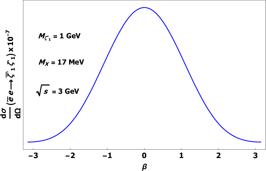
Refer to caption
Figure 12: The differential cross section of e+​e−→ζ¯1′​ζ1′e^{+}\,e^{-}\,\rightarrow\,\bar{\zeta}^{\prime}_{1}\,\zeta^{\prime}_{1} as function of the β\beta-angle. We use the masses Mζ1′=1​GeVM_{\zeta^{\prime}_{1}}=1\,\mbox{GeV} and MX=17​MeVM_{X}=17\,\mbox{MeV}, the CM-energy as s=3​GeV\sqrt{s}=3\,\mbox{GeV}.

The corresponding total cross section is obtained upon integration over the solid angle:

σ⁡(e+​e−→ζ¯1′​ζ1′)=42​π​α2s​εeL2​εζL2(1−MX2/s)2​(1−47​Mζ1′2s).\displaystyle\sigma(e^{+}\,e^{-}\,\rightarrow\,\bar{\zeta}^{\prime}_{1}\,\zeta^{\prime}_{1})=\frac{42\pi\,\alpha^{2}}{s}\frac{\varepsilon_{e_{L}}^{2}\,\varepsilon_{\zeta_{L}}^{2}}{\left(1-M_{X}^{2}/s\right)^{2}}\left(1-\frac{4}{7}\frac{M_{\zeta^{\prime}_{1}}^{2}}{s}\right)\;. (7.8)

Using the previous masses, the C.M. energy of s=3​GeV\sqrt{s}=3\,\mbox{GeV} and |εeL|≲4×10⁻³|\varepsilon_{e_{L}}|\lesssim 4\times 10^{-3}, the σ\sigma-function has the following estimate

σ⁡(e+​e−→ζ¯1′​ζ1′)=1.2× 10−11​εζL2​GeV−2.\displaystyle\sigma(e^{+}\,e^{-}\,\rightarrow\,\bar{\zeta}^{\prime}_{1}\,\zeta^{\prime}_{1})=1.2\,\times\,10^{-11}\,\varepsilon_{\zeta_{L}}^{2}\,\mbox{GeV}^{-2}\;. (7.9)

7.3 The electron and muon g−2g-2 factors

The g−2g-2 factor is an important experimental physical quantity to estimate the ε\varepsilon-parameters of the leptonic sector in interaction with the XX-boson. With those, we can obtain the form factors associated to the vertex ℓ±\ell^{\pm}-photon including the correction of the XX-boson propagator. This correction is illustrated in the figure (13).

0,-0.7)(7,3.5) pscoil[coilarm=0,coilaspect=0,coilwidth=0.5,coilheight=1.0,linecolor=black](1,2)(5,2) pscoil[coilarm=0.35,coilwidth=0.5,coilheight=1,linecolor=black](7,0)(7,4) = q - p ′ p k p p ′ + k p + k p ′

Figure 13: The one-loop correction of the XX-boson to the QED vertex diagram.

With that, we write the QED vertex of lepton-photon corrected by the diagram (13) as the sum : Γμ​(p,p′)=ΓQ​E​Dμ​(p,p′)+Λμ​(p,p′)\Gamma^{\mu}(p,p^{\prime})=\Gamma_{QED}^{\mu}(p,p^{\prime})+\Lambda^{\mu}(p,p^{\prime}). The diagram is represented by the loop 44-momentum integral:

Λμ​(p,p′)\displaystyle\Lambda^{\mu}(p,p^{\prime}) =\displaystyle= ∫d4​k(2​π)4ieγα(cVℓ−cAℓγ5)i(/k+/p′+m)(k+p′)2−m2(ieγμ)×\displaystyle\int\frac{d^{4}k}{(2\pi)^{4}}\,i\,e\,\gamma_{\alpha}\left(c_{V}^{\ell}-c_{A}^{\ell}\,\gamma_{5}\right)\frac{i\left(/\penalty{\!\!\!k}+/\penalty{\!\!\!p}^{\prime}+m\right)}{(k+p^{\prime})^{2}-m^{2}}\left(\,i\,e\,\gamma^{\mu}\,\right)\,\times (7.10)
×i(/k+/p+m)(k+p)2−m2​i​e​γα​(cVℓ−cAℓ​γ5)​−ik2−MX2,\displaystyle\times\,\frac{i\left(/\penalty{\!\!\!k}+/\penalty{\!\!\!p}+m\right)}{(k+p)^{2}-m^{2}}\,i\,e\,\gamma^{\alpha}\left(c_{V}^{\ell}-c_{A}^{\ell}\,\gamma_{5}\right)\frac{-i}{k^{2}-M_{X}^{2}}\;,

where mm stands for the electron or muon mass. Obviously, the integral is divergent in the ultraviolet regime, but we are interested in its finite part. To simplify the previous integral, we use here that the vector coefficient is of the same order of the axial coefficient for Leptons, i. e., cVℓ≃cAℓ=−χcosθW=−εℓL/2=+εℓRc_{V}^{\ell}\simeq c_{A}^{\ell}=-\chi\,\cos\theta_{W}=-\varepsilon_{\ell_{L}}/2=+\varepsilon_{\ell_{R}}. The integral can be calculated by using the known methods of Feynman integrals; then, the finite part of the vertex can be extracted and gives the leptonic current u¯​Γμ​(q)​u\bar{u}\Gamma^{\mu}(q)u, that can be written as

Je​mμ=u¯​(p′)​Γμ​(q)​u​(p)=u¯​(p′)​[F1​(q2)​γμ+F2​(q2)​γ5​γμ+F3​(q2)​i​σμ​ν​qν2​m+F4​(q2)​qμ​γ52​m]​u​(p),J^{\mu}_{em}=\bar{u}(p^{\prime})\Gamma^{\mu}(q)u(p)=\bar{u}(p^{\prime})\left[F_{1}\left(q^{2}\right)\gamma^{\mu}+F_{2}(q^{2})\,\gamma^{5}\gamma^{\mu}+F_{3}(q^{2})\,i\,\frac{\sigma^{\mu\nu}q_{\nu}}{2m}+F_{4}(q^{2})\,\frac{q^{\mu}\gamma^{5}}{2m}\right]u(p)\;, (7.11)

where qμq^{\mu} stands for the momentum transfer and ℓμ=pμ+p′μ\ell^{\mu}=p^{\mu}+p^{\prime\,\mu}, as before. Here, we obtain the QED form factors with the correction of ε\varepsilon-parameters

F1​(q2)\displaystyle F_{1}(q^{2}) =\displaystyle= F1Q​E​D(q2)+α​εℓL24​π∫01dxdydzδ(x+y+z−1)×\displaystyle F_{1}^{QED}(q^{2})+\frac{\alpha\,\varepsilon_{\ell_{L}}^{2}}{4\pi}\int_{0}^{1}dxdydz\,\delta(x+y+z-1)\,\times (7.12)
×4​z−1−z2−(1−x)​(1−y)​q2/m2(1−z)2+z​MX2/m2−x​y​q2/m2,\displaystyle\times\,\frac{4z-1-z^{2}-(1-x)(1-y)q^{2}/m^{2}}{(1-z)^{2}+zM_{X}^{2}/m^{2}-xyq^{2}/m^{2}}\;,

and

F3​(q2)\displaystyle F_{3}(q^{2}) =\displaystyle= α2​π​∫01d​x​𝑑y​𝑑z​δ​(x+y+z−1)​2​z​(1−z)(1−z)2−x​y​q2/m2\displaystyle\frac{\alpha}{2\pi}\int_{0}^{1}dxdydz\,\delta(x+y+z-1)\,\frac{2z(1-z)}{(1-z)^{2}-xy\,q^{2}/m^{2}} (7.13)
−α​εℓL216​π2∫01dxdydzδ(x+y+z−1)2​z​(1−z)(1−z)2+z​MX2/m2−x​y​q2/m2.\displaystyle\hskip-34.14322pt-\frac{\alpha\,\varepsilon_{\ell_{L}}^{2}}{16\pi^{2}}\int_{0}^{1}dxdydz\,\delta(x+y+z-1)\,\frac{2z(1-z)}{(1-z)^{2}+zM_{X}^{2}/m^{2}-xy\,q^{2}/m^{2}}\;.

The F2F_{2} form factor is associated with the CP-violation of the XX-fermion coupling. The conservation current yields us the condition : F2(q2)=−q2F4(q2)/4m2F_{2}(q^{2})=-q^{2}\,F_{4}(q^{2})/4m^{2}; in which the current (7.11) can be rewritten as

Je​mμ=u¯​(p′)​Γμ​(q)​u​(p)=u¯​(p′)​[F1​(q2)​γμ+F4​(q2)​γ5​(qμ/q−q2​γμ)+F3​(q2)​i​σμ​ν​qν2​m]​u​(p),J^{\mu}_{em}=\bar{u}(p^{\prime})\Gamma^{\mu}(q)u(p)=\bar{u}(p^{\prime})\left[F_{1}\left(q^{2}\right)\gamma^{\mu}+F_{4}(q^{2})\,\gamma^{5}\left(q^{\mu}\,/\penalty{\!\!\!q}-q^{2}\gamma^{\mu}\right)+F_{3}(q^{2})\,i\,\frac{\sigma^{\mu\nu}q_{\nu}}{2m}\right]u(p)\;, (7.14)

Explicitly, we have the anapole term with the FAF_{A}-form factor given by

FA​(q2)=F4​(q2)2​m=α​εℓL28​π​∫01d​x​𝑑y​𝑑z​δ​(x+y+z−1)​1+z−(x−y)2(1−z)2+z​MX2/m2−x​y​q2/m2.F_{A}(q^{2})=\frac{F_{4}(q^{2})}{2m}=\frac{\alpha\,\varepsilon_{\ell_{L}}^{2}}{8\pi}\int_{0}^{1}dxdydz\,\delta(x+y+z-1)\,\frac{1+z-(x-y)^{2}}{(1-z)^{2}+zM_{X}^{2}/m^{2}-xy\,q^{2}/m^{2}}\;. (7.15)

The interesting analysis now is the situation where q2=0q^{2}=0 for the external photon in the form factor F3F_{3}. The first term yields the (g−2)ℓ(g-2)_{\ell} factor for the lepton with the correction of the cVℓc_{V}^{\ell} coefficient, which in turn, depends on εℓ\varepsilon_{\ell}-parameters. For the electron case, the F3​(0)F_{3}(0) is given by

F3e​(0)≃α2​π​(1−εeL212​π​me2MX2),\displaystyle F_{3}^{e}(0)\simeq\frac{\alpha}{2\pi}\left(1-\frac{\varepsilon_{e_{L}}^{2}}{12\pi}\,\frac{m_{e}^{2}}{M_{X}^{2}}\right)\;, (7.16)

where we have used that MX≫meM_{X}\gg m_{e}. Using the (g−2)e(g-2)_{e} uncertainty in the literature, we obtain the upper bound on εeL\varepsilon_{e_{L}}-parameter

|εeL|≲ 5.3× 10−5,\displaystyle|\varepsilon_{e_{L}}|\,\lesssim\,5.3\,\times\,10^{-5}\;, (7.17)

and, thus, we estimate the other parameters |εeR|≲ 2.6× 10−5|\varepsilon_{e_{R}}|\,\lesssim\,2.6\,\times\,10^{-5} and |χ|≲ 3× 10−5|\chi|\,\lesssim\,3\,\times\,10^{-5}. For the muon, we obtain

F3μ​(0)≃α2​π​(1−εμL28​π),\displaystyle F_{3}^{\mu}(0)\simeq\frac{\alpha}{2\pi}\left(1-\frac{\varepsilon_{\mu_{L}}^{2}}{8\pi}\right)\;, (7.18)

and using the corresponding (g−2)μ(g-2)_{\mu} uncertainty, we obtain the following upper bound

|εμL|≲ 8.7× 10−5.\displaystyle|\varepsilon_{\mu_{L}}|\,\lesssim\,8.7\,\times\,10^{-5}\;. (7.19)

8 Concluding Comments

We have made efforts to discuss a model with an extra U​(1)KU(1)_{K}-factor that may describe a possible scenario of a Particle Physics beyond the Standard Model (SM). The proposal is based on the gauge group S​UL​(2)×UR​(1)J×U​(1)KSU_{L}(2)\times U_{R}(1)_{J}\times U(1)_{K}, where the extra U​(1)KU(1)_{K}-factor introduces a (new) massive and neutral vector boson. The mass of the latter is generated upon a spontaneous symmetry breaking mechanism that defines an extra VEV scale, beyond that VEV of 246​GeV246\,\mbox{GeV} associated with the usual Higgs field of SM. In our model, the Higgs sector displays two scalar fields and the gauge symmetry allows interactions between them. This mechanism can be introduced in two ways : in the first case, the SSB pattern-I takes place through a VEV scale-uu, where u>246​GeVu>246\,\mbox{GeV}, and, as consequence, we fix a mass for the hypothetical Z′Z^{\prime}-boson around 2 TeV. Next, the SM Higgs acquires its VEV of 246​GeV246\,\mbox{GeV}, breaks the electroweak symmetry to give the masses for W±W^{\pm} and ZZ. The sequence of SSB mechanism is as follows:

S​UL×UR​(1)J×U​(1)K⟼⟨Ξ⟩0S​UL​(2)×UY​(1)⟼⟨Φ⟩0Ue​m​(1).\displaystyle SU_{L}\!\times\!U_{R}(1)_{J}\!\times\!U(1)_{K}\stackrel{{\scriptstyle\langle\Xi\rangle_{0}}}{{\longmapsto}}SU_{L}(2)\!\times\!U_{Y}(1)\stackrel{{\scriptstyle\langle\Phi\rangle_{0}}}{{\longmapsto}}U_{em}(1)\;.

The result for the mass of Z′Z^{\prime} is estimated by the ATLAS and CMS Collaborations as a possible particle at the TeV-scale. The maximum VEV scale for MZ′=2​TeVM_{Z^{\prime}}=2\,\mbox{TeV} is u=2.8​TeVu=2.8\,\mbox{TeV}, and it allows an estimation of the mass of the new Higgs within the range 1.2​TeV<MF<3.7​TeV1.2\,\mbox{TeV}<M_{F}<3.7\,\mbox{TeV}. Furthermore, the subgroup U​(1)KU(1)_{K} also introduces a new family of fermions in the TEV-scale, which we call ζi\zeta_{i}-fermions (i=1,2,3)(i=1,2,3), that could be candidates to the dark matter particles. It is a set of neutral heavy fermions associated with the VEV scale of 2.8​TeV2.8\,\mbox{TeV} and they guarantee that model be free from the chiral anomaly. We use the masses for ζi\zeta_{i} in the range of 0.5−1​TeV0.5-1\,\mbox{TeV}, motivated by recent simulations of dark matter fermions scenario in the CMS-Collaboration. Furthermore, these new fermions also mix with a Dirac’s right-neutrino component. This new mixing motivated us to investigate the MDM of the ζi\zeta_{i}-fermions, and the transition MDMs of the ζi\zeta_{i} mixed with neutrinos. Since ζi\zeta_{i} are neutral fermions, their MDMs depend on their masses and also on the mixing with the right-neutrinos. At one-loop, the diagonal ζ1\zeta_{1}-MDM for mass of 0.5​TeV0.5\,\mbox{TeV} is estimated by μM(ζ1′)=1.2× 10−21​μB\mu_{M}^{(\zeta^{\prime}_{1})}=1.2\,\times\,10^{-21}\,\mu_{B}.

In the second scenario, the SSB mechanism pattern-II is introduced to break the composite subgroup S​UL​(2)×UR​(1)JSU_{L}(2)\times U_{R}(1)_{J} in the VEV scale of the SM, 246​GeV246\,\mbox{GeV}, to yield the usual ZZ-mass, and so, a further SBB defines the VEV scale-uu, u<246​GeVu<246\,\mbox{GeV}. In this second situation, we have the scenario of a lighter extra gauge boson; it may describe a phenomenology of elementary particle physics at a lower energy scale. The scheme for the pattern-II SSB is displayed below:

S​UL×UR​(1)J×U​(1)K⟼⟨Φ⟩0U​(1)G×U​(1)K⟼⟨Ξ⟩0U​(1)e​m.\displaystyle SU_{L}\times U_{R}(1)_{J}\times U(1)_{K}\stackrel{{\scriptstyle\langle\Phi\rangle_{0}}}{{\longmapsto}}U(1)_{G}\times U(1)_{K}\stackrel{{\scriptstyle\langle\Xi\rangle_{0}}}{{\longmapsto}}U(1)_{em}\;.

This proposal may be discussed in connection with the light X-Boson, dark photon or para-photon phenomenology, at MeV-scale or lower, which can be related to dark matter particles. This context includes the recent description of a new boson needed to explain the excited 88-Beryllium nuclear decay. In this case, the mass of the XX-Boson is fixed at the mass scale of mX=17​MeVm_{X}=17\,\mbox{MeV}. Therefore, the results of SSB lead us to the VEV scale of u≃1.9−19​GeVu\simeq 1.9-19\,\mbox{GeV} that must be origin of a hidden Higgs within the range mass 1.9​GeV≲MF≲19​GeV1.9\,\mbox{GeV}\lesssim M_{F}\lesssim 19\,\mbox{GeV}. In this context, the ζi\zeta_{i}-fermions are interpreted as light particles with masses in the range of 0.3−6.6​GeV0.3-6.6\,\mbox{GeV}. It can be a candidate to dark matter constituent. After the SSB pattern-II, we study the phenomenology of the XX-Boson through its decay into electron, neutrino and light uu-quark, and the scattering e+​e−→X→ζ¯1′​ζ1′e^{+}\,e^{-}\rightarrow X\rightarrow\bar{\zeta}^{\prime}_{1}\,\zeta^{\prime}_{1}, with Mζ1′=1​GeVM_{\zeta^{\prime}_{1}}=1\,\mbox{GeV}; this can connect the SM with the dark sector with a hidden photon mediating the interaction. To conclude, we calculate the correction to the Quantum Electrodynamics (QED) vertex due to axial interaction of XX-Boson with the leptons of the SM; in particular, for the electron and muon cases. The results impose the bounds |εeL|≲ 5.3× 10−5|\varepsilon_{e_{L}}|\,\lesssim\,5.3\,\times\,10^{-5} and |εμL|≲ 8.7× 10−5|\varepsilon_{\mu_{L}}|\,\lesssim\,8.7\,\times\,10^{-5} for the electron and muon, respectively, which measures the magnitude of the weak interaction of the electron/muon with the XX-Boson. The Electric Dipole Momentum of the charged leptons must emerge at higher loop orders, in both cases of the Z′Z^{\prime} and XX-boson scenarios. This is an issue we are now investigating and we shall report on it in a further paper.

A unification scheme including W′W^{\prime}- and Z′Z^{\prime}-bosons is in the framework of an left-right symmetric model S​UL​(2)×S​UR​(2)×U​(1)J×U​(1)KSU_{L}(2)\times SU_{R}(2)\times U(1)_{J}\times U(1)_{K} may also be the subject of a further investigation to be pursued in the presence of dark matter fermion content.

References

  • (1) ATLAS Collaboration, Phys. Rev. D 90, no. 5, 052005 (2014).
  • (2) The CMS Collaboration, JHEP 1504, 025 (2015).
  • (3) The CMS Collaboration, Phys. Lett. B, 2017, 773, 563.
  • (4) The CMS Collaboration, J. High Energy Phys., 2017, 07, 014.
  • (5) The CMS Collaboration, Search for new physics in final states with an energetic jet or a hadronically decaying W or Z boson and transverse momentum imbalance at s=13\sqrt{s}=13 TeV, Arxiv : 1712.02345.
  • (6) Bogdan A. Dobrescu and Zhen Liu, JHEP (2015) 2015 : 118.
  • (7) Bogdan A. Dobrescu and Zhen Liu, Phys. Rev. Lett. 115 (2015) 211802.
  • (8) P. Coloma, B. A. Dobrescu and J. Lopez-Pavon, Phys. Rev. D 92 (2015) 115023.
  • (9) Bogdan A. Dobrescu and Patrick J. Fox, JHEP (2016) 2016 : 047.
  • (10) P. S. Bhupal Dev and R. N. Mohapatra, Phys. Rev. Lett. 115 (2015) 181803.
  • (11) S. Patra, W. Rodejohann and C. E. Yaguna JHEP (2016) 2016 : 076.
  • (12) Pei-Hong Gu and Rabindra N. Mohapatra, Phys. Rev. D 96, 055011 (2017).
  • (13) P. S. Bhupal Dev, Rabindra N. Mohapatra and Yongchao Zhang, Journal of Physics : Conf. Series 873 (2017) 012029.
  • (14) Paul Langacker, Reviews of Modern Physics, 81 (2009) 1199-1228.
  • (15) Shinya Kanemura, Osamu Seto and Takashi Shimomura, Phys. Rev. D 84 (2011) 016004.
  • (16) E. Accomano et al, JHEP (2016) 2016 : 86.
  • (17) A. J. Krasznahorkay et al, Phys. Rev. Lett. 116 (2016) 042501.
  • (18) J. L. Feng et al, Phys. Rev. Lett. 117 (2016) 071803.
  • (19) Pei-Hong Gu , Xiao-Gang He, Nuclear Physics B 919 (2017) 209-217.
  • (20) J. L. Feng et al, Phys. Rev. D 95, 035017 (2017).
  • (21) Yonathan Kahn, Gordan Krnjaic, Siddharth Mishra-Sharma, Tim M. P. Tait, J. High Energy Phys., 2017, 05, 002.
  • (22) S. Bilmis, I. Turan, T. M. Aliev, M. Deniz, L. Singh, H. T. Wong, Phys. Rev. D 2015, 92, 033009.
  • (23) Teppei Kitahara and Yasuhiro Yamamoto, Phys. Rev. D 95, 015008 (2017).
  • (24) J. P. Lees et al. (BaBar Collaboration), Phys. Rev. Lett. 119 (2017) 131804.
  • (25) M. Ahlers, H. Gies, J. Jaeckel, J. Redondo, and A. Ringwald, Phys. Rev. D 76 (2007) 115005.
  • (26) J. Jaeckel, A. Ringwald, Phys. Lett. B 659 (2008) 509-514.
  • (27) P. Arias, J. Jaeckel, J. Redondo, and A. Ringwald, Phys. Rev. D 82 (2016) 115018.
  • (28) M. J. Neves and J. A. Helayël-Neto, Annalen Der Physik 2017, 1700112.
  • (29) Nicole F. Bell et. al., Phys. Rev. Lett. 95 (2005) 151802.
  • (30) Nicole F. Bell et. al., Phys. Lett. B 642 (2006) 377-383.
  • (31) Kaushik Bhattacharya and Palash B Pal, Proc Indian Natn Sci Acad, 70, A No. 1, January 2004, pp. 145–161.
  • (32) A. B. Balantekin, AIP Conference Proceedings 847, 128 (2006).
  • (33) Alexander Studenikin, Journal of Physics : Conference Series 718 (2016) 062076.
  • (34) C. Patrignani et. al. (Particle Data Group), Chin. Phys. C 40 100001 (2016).
  • (35) M. Duerr and P. Fileviez Perez, Phys. Lett. B 732 101 (2014).
  • (36) M. Duerr and P. Fileviez Perez, Phys. Rev. D 91 (2015) 095001.
  • (37) Jonathan Kozaczuk, David E. Morrissey, S. R. Stroberg, Phys. Rev. D 2017, 95, 115024.
  • (38) H. Davoudiasl, H. -S. Lee and W. J. Marciano, Phys. Rev. D 89, 095006 (2014).
  • (39) M. Raggi et al. (NA48/2 Collaboration), NA48/2 studies of rare decays, Nuovo Cimento Soc. Ital. Fis. 38, 132 (2016).
  • (40) KamLAND Collaboration, Phys. Rev. Lett., 2005, 94, 081801.
  • (41) Subinoy Das, Kris Sigurdson, Phys. Rev. D 2012, 85, 063510.
  • (42) KLOE Collaboration, Phys. Lett. B, 2016, 757, 362.