跳到论文正文
W Papers独立论文阅读器 arXiv:1611.07916 论文正文 计算阅读时间 · 0%
引用这篇论文根据当前论文元数据生成,正式投稿前建议核对。


License: arXiv.org perpetual non-exclusive license
arXiv:1611.07916v1 [math.GT] 23 Nov 2016

Perturbed gradient flow trees and A∞A_{\infty}-algebra structures on Morse cochain complexes

Stephan Mescher Address: School of Mathematical Sciences
Queen Mary University of London
Mile End Road
London E1 4NS
Email address: s.mescher@qmul.ac.uk
Date: August 24, 2026
Abstract.

We elaborate on an idea of M. Abouzaid of equipping the Morse cochain complex of a smooth Morse function on a closed oriented manifold with the structure of an A∞A_{\infty}-algebra. This is a variation on K. Fukaya’s definition of Morse-A∞A_{\infty}-categories for closed oriented manifolds involving families of Morse functions. The purpose of this article is to provide a coherent and detailed treatment of Abouzaid’s approach including a discussion of all relevant analytic notions and results.

Introduction

Morse (co)homology

The upshot of the construction of Morse homology is that with every complete finite-dimensional manifold MM and every Morse function f:M→ℝf:M\to\mathbb{R} which is bounded from below one can associate a chain complex of free abelian groups generated by the critical points of ff. We denote this complex by

C∗​(f):=⨁x∈Crit ⁡fℤ⋅x,whereCj​(f)=⨁μMorse​(x,f)=jℤ⋅x.C_{*}(f):=\bigoplus_{x\in\Crit f}\mathbb{Z}\cdot x\ ,\quad\text{where}\ \ C_{j}(f)=\bigoplus_{\mu_{\text{Morse}}(x,f)=j}\mathbb{Z}\cdot x\ .

Here, Crit ⁡f⊂M\Crit f\subset M denotes the set of critical points of a Morse function and μMorse\mu_{\text{Morse}} denotes the Morse index of a critical point. Since the Morse index is bounded from below by zero and from above by the dimension of MM, the group Cj​(f)C_{j}(f) is only non-zero if j∈{0,1,…,n}j\in\{0,1,\dots,n\}.

A differential on C∗​(f)C_{*}(f) is defined via counting elements of zero-dimensional moduli spaces of negative gradient flow trajectories. More precisely, for x,y∈Crit ⁡fx,y\in\Crit f we define

ℳ(x,y,g):={γ:ℝ⟶C∞M|γ˙=−(∇gf)∘γ,lims→−∞γ(s)=x,lims→+∞γ(s)=y},\mathcal{M}(x,y,g):=\Bigl\{\gamma:\mathbb{R}\stackrel{{\scriptstyle C^{\infty}}}{{\longrightarrow}}M\ \Big|\ \dot{\gamma}=-(\nabla^{g}f)\circ\gamma,\ \lim_{s\to-\infty}\gamma(s)=x,\ \lim_{s\to+\infty}\gamma(s)=y\Big\}\ ,

where gg is a Riemannian metric on MM and ∇gf\nabla^{g}f denotes the gradient vector field of ff with respect to gg. It is shown in [Sch93] that for generic choice of gg, this space is a smooth manifold of dimension μ⁡(x)−μ⁡(y)\mu(x)-\mu(y) for any such xx and yy. Moreover, the reparametrization ℝ×ℳ⁡(x,y,g)→ℳ⁡(x,y,g)\mathbb{R}\times\mathcal{M}(x,y,g)\to\mathcal{M}(x,y,g), (s,γ)↦γ(⋅+s)(s,\gamma)\mapsto\gamma(\cdot+s), is a smooth, free and proper ℝ\mathbb{R}-action on ℳ⁡(x,y,g)\mathcal{M}(x,y,g) whenever x≠yx\neq y, implying that the quotient space by this group action, the space of unparametrized flow lines from xx to yy

ℳ^​(x,y,g):=ℳ⁡(x,y,g)/ℝ,\widehat{\mathcal{M}}(x,y,g):=\mathcal{M}(x,y,g)/\mathbb{R}\ ,

is a manifold of dimension μ⁡(x)−μ⁡(y)−1\mu(x)-\mu(y)-1. Moreover, it is shown in [Sch93] that if μ⁡(x)=μ⁡(y)+1\mu(x)=\mu(y)+1, the space ℳ^​(x,y,g)\widehat{\mathcal{M}}(x,y,g) is a finite set and we can use certain orientation constructions to define an algebraic count of elements of ℳ^​(x,y,g)\widehat{\mathcal{M}}(x,y,g). Define this number by n⁡(x,y,g):=#alg​ℳ^​(x,y,g)n(x,y,g):=\#_{\text{alg}}\widehat{\mathcal{M}}(x,y,g).

For a generically chosen metric gg, the differential on C∗​(f)C_{*}(f) is then defined by

∂g:C∗​(f)→C∗−1​(f),(x∈Crit ⁡f)↦∑μ⁡(y)=μ⁡(x)−1y∈Crit ⁡fn⁡(x,y,g)⋅y,\partial^{g}:C_{*}(f)\to C_{*-1}(f)\ ,\quad(x\in\Crit f)\mapsto\sum_{\stackrel{{\scriptstyle y\in\Crit f}}{{\mu(y)=\mu(x)-1}}}n(x,y,g)\cdot y\ ,

and by extending this definition ℤ\mathbb{Z}-linearly to all of C∗​(f)C_{*}(f).

There is also the dual notion of Morse cohomology. The Morse cochain complex is defined by

C∗​(f):=∏x∈Crit ⁡fℤ⋅x,whereCj​(f)=∏μMorse​(x,f)=jℤ⋅x,\displaystyle C^{*}(f):=\prod_{x\in\Crit f}\mathbb{Z}\cdot x\ ,\quad\text{where}\ \ C^{j}(f)=\prod_{\mu_{\text{Morse}}(x,f)=j}\mathbb{Z}\cdot x\ ,
δg:C∗​(f)→C∗+1​(f),(x∈Crit ⁡f)↦∑μ⁡(z)=μ⁡(x)+1z∈Crit ⁡fn⁡(z,x,g)⋅z,\displaystyle\delta^{g}:C^{*}(f)\to C^{*+1}(f)\ ,\quad(x\in\Crit f)\mapsto\sum_{\stackrel{{\scriptstyle z\in\Crit f}}{{\mu(z)=\mu(x)+1}}}n(z,x,g)\cdot z\ ,

and by extending the codifferential ℤ\mathbb{Z}-linearly to C∗​(f)C^{*}(f). The duality between the Morse chain and cochain complex is obvious.

By considering compactifications of one-dimensional spaces of unparametrized flow lines, one shows that indeed ∂g∘∂g=0\partial^{g}\circ\partial^{g}=0 and δg∘δg=0\delta^{g}\circ\delta^{g}=0. Moreover, the (co)homology of these complexes is isomorphic to singular (co)homology with integer coefficients:

H∗​(f)≅H∗sing​(M,ℤ),H∗​(f)≅Hsing∗​(M,ℤ),H_{*}(f)\cong H^{\text{sing}}_{*}(M;\mathbb{Z})\ ,\quad H^{*}(f)\cong H^{*}_{\text{sing}}(M;\mathbb{Z})\ ,

where H∗(f):=H∗(C∗(f),∂g)H_{*}(f):=H_{*}(C_{*}(f),\partial^{g}) and H∗​(f):=H∗​(C∗​(f),δg)H^{*}(f):=H^{*}(C^{*}(f),\delta^{g}). In particular, the (co)homolo gy of the Morse (co)chain complex is independent of the choice of the Morse function and the Riemannian metric. The original proof of this statement is spread throughout the literature and usually attributed to Thom, Smale and Witten.

A∞A_{\infty}-categories of Morse cochain complexes

Having realized the singular cohomology of a manifold in terms of Morse theory, it is natural to ask whether the cup product of singular cohomology possesses a Morse-theoretic realization as well. The answer is yes and such a description of the cup product was discovered by Kenji Fukaya, as well as a family of higher order multiplications on Morse cochain complexes

C∗​(f1)⊗C∗​(f2)⊗⋯⊗C∗​(fd)→C∗​(f0)C^{*}(f_{1})\otimes C^{*}(f_{2})\otimes\dots\otimes C^{*}(f_{d})\to C^{*}(f_{0})

for every d≥2d\geq 2, where f0,f1,…,fd∈C∞​(M)f_{0},f_{1},\dots,f_{d}\in C^{\infty}(M) are Morse functions and MM is a closed oriented manifold.

These higher order multiplications had their first appearance in [Fuk93] and were further elaborated on in [Fuk97]. The analytic details were carried out by Fukaya and Yong-Geun Oh in [FO97]. See also [Abo09] for a generalization to compact manifolds with boundary.

However, there is a huge difference between the singular and the Morse-theoretic cup product. The singular one has the property of being associative on the level of cochains, while the Morse-theoretic one is not associative on the cochain level. Indeed, Fukaya has shown that the family of higher order multiplications satisfies the A∞A_{\infty}-equations.

A technical difficulty that occurs is that the multiplications are maps from the product of the Morse cochain complexes of dd different Morse functions instead of the dd-fold product of the Morse cochain complex of a single Morse function. Here, it is not possible to choose the same Morse function in every factor. To understand this, we have to delve deeper into the definitions of the higher order multiplications.

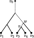
Similar to the Morse differential and codifferential, the higher order multiplications are defined via counting elements of zero-dimensional moduli spaces. For d≥2d\geq 2, these moduli spaces consist of continuous maps from a rooted tree (seen as a one-dimensional CW complex) to the manifold MM which map the root and the leaves of the tree to fixed critical points, while they edgewise fulfill negative gradient flow equations. For example, let fi∈C∞​(M)f_{i}\in C^{\infty}(M), xi∈Crit ⁡fix_{i}\in\Crit f_{i} for i∈{0,1,…,d}i\in\{0,1,\dots,d\} and TT be a dd-leafed rooted binary tree. We consider maps I:T→MI:T\to M with I⁡(vi)=xiI(v_{i})=x_{i} for every ii, where v0v_{0} denotes the root and viv_{i} denotes the ii-th leaf of TT for every i∈{1,2,…,d}i\in\{1,2,\dots,d\}. Moreover, we want that for every edge ee there is a Morse function fef_{e} such that

I˙e=−(∇gfe)∘Ie\dot{I}_{e}=-(\nabla^{g}f_{e})\circ I_{e}

where IeI_{e} denotes the restriction of II to ee. (The edges of TT will be parametrized by suitable intervals.) The property of the corresponding moduli spaces being smooth manifolds can be rephrased as a transverse intersection problem. Therefore, the Morse functions involved have to satisfy certain transversality conditions which make it impossible to choose f1=⋯=fdf_{1}=\dots=f_{d}.

Fukaya’s method is to start with arbitrary, but distinct, Morse functions associated with every edge leading to a leaf of TT. For every other edge ee we define fef_{e} as the sum of the functions fe′f_{e^{\prime}} for every e′e^{\prime} whose incoming vertex coincides with the outgoing vertex of ee. For a generic choice of Riemannian metric gg, the corresponding moduli space is then a smooth manifold.

For example, the multiplication for d=2d=2, which is nothing but the cochain-level cup product, is defined as a map

C∗​(f1)⊗C∗​(f2)→C∗​(f1+f2),C^{*}(f_{1})\otimes C^{*}(f_{2})\to C^{*}(f_{1}+f_{2})\ ,

if f1f_{1}, f2f_{2} and f1+f2f_{1}+f_{2} are Morse functions on MM. Using these properties, Fukaya was able to define an A∞A_{\infty}-category whose objects are smooth functions on MM and whose morphism sets are Morse cochain complexes.

Abouzaid’s approach: perturbing gradient flow lines

In several situations, for example if one is interested in the Hochschild homology of Morse cochain complexes, it is difficult to work with an A∞A_{\infty}-category due to the presence of infinitely many cochain complexes as objects. Instead, it is preferrable to work with an A∞A_{\infty}-algebra, i.e. an A∞A_{\infty}-category that has precisely one object, see [Mes16b]. Such a construction is provided by an alternative approach to Fukaya’s A∞A_{\infty}-structures in Morse theory, which was suggested by Mohammed Abouzaid in [Abo11]. Abouzaid defines products C∗​(f)⊗d→C∗​(f)C^{*}(f)^{\otimes d}\to C^{*}(f) for a closed oriented manifold MM, a fixed Morse function f:M→ℝf:M\to\mathbb{R} and every d≥2d\geq 2 by considering moduli spaces of continuous maps from a tree to the manifold, which are trajectories of perturbations of the negative gradient flow of a Morse function on a closed manifold. Using transversality theory, one shows that for generic choices of perturbations, the resulting moduli spaces will be manifolds. Then one can construct the higher order multiplications along the same lines as in Fukaya’s works by counting elements of zero-dimensional moduli spaces.

Abouzaid has shown that for good choices of perturbations, the Morse cochain complex C∗​(f)C^{*}(f) with the resulting higher order multiplications becomes an A∞A_{\infty}-algebra. Moreover, his results imply that the Hochschild homology of this A∞A_{\infty}-algebra is independent of the choices of perturbations and isomorphic to the Hochschild homology of the singular cochains of the manifold.

In fact, Abouzaid’s perturbation method is the Morse-theoretic analogue of the more sophisticated Floer-theoretic perturbations constructed by Paul Seidel in [Sei08, Part II]. Seidel defined perturbations for pseudo-holomorphic curves which are modelled on boundary-pointed disks, which require more subtle analytic methods, especially concerning compactness properties of the resulting moduli spaces.

The aim of this article is to give a detailed construction of the higher order multiplications on the Morse cochains of a fixed Morse function using the perturbation methods of Abouzaid. Moreover, we want to show that for convenient choices of perturbations the Morse cochain complex equipped with these multiplications becomes an A∞A_{\infty}-algebra. We will provide the reader with many analytic details and a self-contained construction of higher order multiplications after Abouzaid’s ideas.

The basic ideas of this article are implicitly contained in [Abo11]. Many of the results are stated or partially proven in Abouazid’s work and we will provide the analytic details underlying Abouzaid’s methods. For the sake of readability, we refrain from giving a reference to the corresponding result in Abouzaid’s work at every result we are considering and see this paragraph as a general reference to [Abo11].

We assume that the reader is familiar with standard results of Morse theory as well as the construction of Morse homology. The classic reference for Morse theory is [Mil63], while newer treatments include [Nic11], [Mat02] and Chapter 6 of [Jos08].

There are also certain references specializing on Morse homology. We will loosely orient our treatment on the textbook [Sch93], which stresses the meaning of Morse trajectory spaces in the construction of Morse homology. Further references include [BH04], which takes a classic differential-topological approach, [Hut02], [Web06] and [AM06].

We assume that the reader is familiar with certain constructions related to Morse homology. Throughout this article and especially in Section 1 we will use several results for spaces of (unperturbed) negative gradient flow trajectories and give references to those results whenever they are needed. Moreover, we will rely on certain gluing analysis results for Morse trajectories which transfer with only minor modifications to our situation. The necessary results are contained in [Sch93], [Sch99] and [Weh12].

Furthermore, Sections 3 to 5 require certain results from graph theory which we will mostly state without providing proofs. The proofs of those results are elementary and therefore left to the reader.

In Section 1, we carefully introduce the necessary spaces of perturbations and the different kinds of perturbed negative gradient flow trajectories. We will rely on certain results on unperturbed negative gradient flow trajectories which we will briefly present. Thereupon, we discuss moduli spaces of these perturbed trajectories and certain evaluation maps defined on the moduli spaces.

The results about the evaluation maps are further generalized in Section 2. After introducing certain more general perturbation spaces, we consider moduli spaces of families of perturbed Morse trajectories satisfying endpoint conditions, which are in a certain sense nonlocal. Finally, we state and prove a general regularity theorem about these moduli spaces.

This nonlocal regularity theorem is applied to a special situation in Section 3. This section starts with the introduction of several notions from graph theory. Afterwards, we discuss how the results from Section 2 can be applied to consider moduli spaces of maps from a tree to a manifold which edgewise fulfill a perturbed negative gradient flow equation.

In Section 4 we investigate sequential compactness properties of the moduli spaces from Section 3. We introduce a notion of geometric convergence with which we can describe the possible limiting behaviour of sequences in the moduli spaces of perturbed negative gradient flow trees. We further give explicit descriptions of the moduli spaces in which the respective limits are lying.

The objects of study in Section 5 are zero- and one-dimensional moduli spaces of perturbed negative gradient flow trees. By applying the results of Section 4 to zero-dimensional spaces we are able to define multiplications on Morse cochain complexes via counting elements of these moduli spaces. Applying the abovementioned gluing results from Morse theory, we will describe compactifications of one-dimensional moduli spaces and finally use the counts of their boundary components to prove that the Morse cochain complex equipped with the multiplications becomes an A∞A_{\infty}-algebra.

A discussion of orientability and orientations of the moduli spaces of perturbed Morse ribbon trees is required in order to construct higher order multiplications with integer coefficients, since they will be constructed by using oriented intersection numbers. For the benefit of the flow of reading, all results about orientations are not contained in the main part of this article, but are found in Appendix A. We will give references to the respective parts of this appendix whenever required.

Throughout this article, let MM be a closed nn-dimensional smooth oriented manifold, n∈ℕ0n\in\mathbb{N}_{0}, and f∈C∞​(M)f\in C^{\infty}(M) be a Morse function. Let Crit ⁡f:={x∈M|d​fx=0}\Crit f:=\{x\in M\ |\ df_{x}=0\} denote the set of critical points of ff and for any x∈Crit ⁡fx\in\Crit f let μ⁡(x)\mu(x) denote its Morse index with respect to ff. We will further use the convention that the empty set is a manifold of every dimension.

Acknowledgements

The contents of this article are part of the author’s Ph. D. thesis [Mes16a], which was submitted to the University of Leipzig and supervised by Prof. Dr. Matthias Schwarz. The author thanks Prof. Schwarz for his guidance and support. Moreover, the author is grateful to Prof. Dr. Alberto Abbondandolo for many helpful discussions.

The author further thanks Dr. Matti Schneider and Dr. Roland Voigt for helpful comments on earlier versions of this article.

1. Perturbations of gradient flow trajectories

We start by repeating some necessary definitions and results from finite-dimensional Morse theory. A discussion of these notions and results can be found in many sources, among them [Jos08, Chapter 6], [Sch99] and [BH04].

Definition 1.1.

Let x∈Crit ⁡fx\in\Crit f. For every Riemannian metric gg on MM, the unstable manifold of xx with respect to (f,g)(f,g) is defined by

Wu​(x,f,g):={y∈M|limt→−∞ϕt−∇gf​(y)=x},W^{u}(x,f,g):=\Bigl\{y\in M\ \Big|\ \lim_{t\to-\infty}\phi^{-\nabla^{g}f}_{t}(y)=x\ \Bigr\}\ ,

where ϕ−∇gf\phi^{-\nabla^{g}f} denotes the flow of the vector field −∇gf-\nabla^{g}f, i.e. the negative gradient flow of ff with respect to gg. The stable manifold of xx with respect to (f,g)(f,g) is defined by

Ws​(x,f,g):={y∈M|limt→+∞ϕt−∇gf​(y)=x}.W^{s}(x,f,g):=\Bigl\{y\in M\ \Big|\ \lim_{t\to+\infty}\phi^{-\nabla^{g}f}_{t}(y)=x\ \Bigr\}\ .

It is well-known from Morse theory, see [Jos08, Section 6.3] or [Web06, Theorem 2.7], that for every x∈Crit ⁡fx\in\Crit f the unstable and stable manifolds of xx with respect to (f,g)(f,g) are smooth manifolds of dimension

dimWu​(x,f,g)=μ⁡(x),dimWs​(x,f,g)=n−μ⁡(x),\dim W^{u}(x,f,g)=\mu(x)\ ,\quad\dim W^{s}(x,f,g)=n-\mu(x)\ ,

respectively, and that both Wu​(x,f,g)W^{u}(x,f,g) and Ws​(x,f,g)W^{s}(x,f,g) are embedded submanifolds of MM. Moreover, MM can be decomposed into the unstable and stable manifolds with respect to (f,g)(f,g):

M=⋃x∈Crit ⁡fWu​(x,f,g)=⋃x∈Crit ⁡fWs​(x,f,g).M=\bigcup_{x\in\Crit f}W^{u}(x,f,g)=\bigcup_{x\in\Crit f}W^{s}(x,f,g)\ .
Definition 1.2.

We call a pair (f,g)(f,g) consisting of a smooth function f∈C∞​(M)f\in C^{\infty}(M) and a smooth Riemannian metric gg on MM a Morse-Smale pair if ff is a Morse function and if Wu​(x,f,g)W^{u}(x,f,g) and Ws​(y,f,g)W^{s}(y,f,g) intersect transversely for all x,y∈Crit ⁡fx,y\in\Crit f.

Equipping the set of smooth Riemannian metrics on MM with a suitable topology, one shows that for any given Morse function f∈C∞​(M)f\in C^{\infty}(M) the set of Riemannian metrics gg for which (f,g)(f,g) is a Morse-Smale pair is a generic subset of the space of Riemannian metrics, see [Sch93, Section 2.3] or [BH04, Section 6.1] for details.

We next want to rephrase the definition of unstable and stable manifolds in terms of spaces of negative half-trajectories as it is done in [Sch99]. This reformulation will be helpful for introducing the notion of perturbed gradient flow half-trajectories. Define

ℝ¯:=ℝ∪{−∞,+∞},ℝ¯≥0:=[0,+∞)∪{+∞},ℝ¯≤0:=(−∞,0]∪{−∞}.\overline{\mathbb{R}}:=\mathbb{R}\cup\{-\infty,+\infty\}\ ,\quad\overline{\mathbb{R}}_{\geq 0}:=[0,+\infty)\cup\{+\infty\}\ ,\quad\overline{\mathbb{R}}_{\leq 0}:=(-\infty,0]\cup\{-\infty\}\ .

In [Sch93, Section 2.1], ℝ¯\overline{\mathbb{R}} is equipped with a smooth structure by choosing a diffeomorphism h:ℝ→(−1,1)h:\mathbb{R}\to(-1,1) with

h⁡(0)=0,lims→−∞h⁡(s)=−1,lims→+∞h⁡(s)=1,h(0)=0\ ,\quad\lim_{s\to-\infty}h(s)=-1\ ,\quad\lim_{s\to+\infty}h(s)=1\ ,

by extending hh in the obvious way to a bijection h:ℝ¯→[−1,1]h:\overline{\mathbb{R}}\to[-1,1] and requiring that this extended map is a diffeomorphism of manifolds with boundary. In the following we always assume such a map hh to be chosen and fixed. We equip ℝ¯≤0\overline{\mathbb{R}}_{\leq 0} and ℝ¯≥0\overline{\mathbb{R}}_{\geq 0} with the unique smooth structures which make them smooth submanifolds with boundary of ℝ¯\overline{\mathbb{R}}.

For a Riemannian metric gg on MM and x∈Crit ⁡fx\in\Crit f define spaces of curves

𝒫−​(x):={γ∈H1​(ℝ¯≤0,M)|lims→−∞γ⁡(s)=x},\displaystyle\mathcal{P}_{-}(x):=\Bigl\{\gamma\in H^{1}\left(\overline{\mathbb{R}}_{\leq 0},M\right)\ \Big|\ \lim_{s\to-\infty}\gamma(s)=x\Bigr\}\ ,
𝒫+​(x):={γ∈H1​(ℝ¯≥0,M)|lims→+∞γ⁡(s)=x},\displaystyle\mathcal{P}_{+}(x):=\Bigl\{\gamma\in H^{1}\left(\overline{\mathbb{R}}_{\geq 0},M\right)\ \Big|\ \lim_{s\to+\infty}\gamma(s)=x\Bigr\}\ ,

where H1H^{1} always denotes spaces of maps of Sobolev class W1,2W^{1,2} with respect to the Riemannian metric gg. These spaces can be equipped with structures of Hilbert manifolds, see [Sch93, Appendix A]. The following spaces can be equipped with structures of Banach bundles over 𝒫−​(x)\mathcal{P}_{-}(x), 𝒫+​(x)\mathcal{P}_{+}(x), respectively, by

ℒ−​(x):=⋃γ∈𝒫−​(x)L2​(γ∗​T​M),ℒ+​(x):=⋃γ∈𝒫+​(x)L2​(γ∗​T​M),\mathcal{L}_{-}(x):=\bigcup_{\gamma\in\mathcal{P}_{-}(x)}L^{2}(\gamma^{*}TM)\ ,\qquad\mathcal{L}_{+}(x):=\bigcup_{\gamma\in\mathcal{P}_{+}(x)}L^{2}(\gamma^{*}TM)\ ,

together with the obvious bundle projections, where L2​(γ∗​T​M)L^{2}(\gamma^{*}TM) denotes the space of sections of the vector bundle γ∗​T​M\gamma^{*}TM which are L2L^{2}-integrable with respect to gg. It can be shown by the methods of [Sch93, Appendix A] that ℒ−​(x)→𝒫−​(x)\mathcal{L}_{-}(x)\to\mathcal{P}_{-}(x) and ℒ+​(x)→𝒫+​(x)\mathcal{L}_{+}(x)\to\mathcal{P}_{+}(x) are indeed smooth Banach bundles over Hilbert manifolds.

The following notion is implicitly used in [Sch93] and [Sch99], though its name seems to have its first appearance in the literature in [HWZ07] in a much more general context. We will use it in our Morse-theoretic framework in the upcoming theorems.

Definition 1.3.

Let MM be a Banach manifold and E→ME\to M be a Banach bundle over MM with typical fiber FF. A section of the bundle s:M→Es:M\to E is called a Fredholm section of index r∈ℤr\in\mathbb{Z}, if there is a local trivialization

{(Uα,φα:E|Uα→≅Uα×F)}α∈I,\left\{\left(U_{\alpha},\varphi_{\alpha}:E|_{U_{\alpha}}\stackrel{{\scriptstyle\cong}}{{\to}}U_{\alpha}\times F\right)\right\}_{\alpha\in I}\ ,

where II is an index set, such that for every α∈I\alpha\in I the map

p​r2∘φα∘s|Uα:Uα→F,pr_{2}\circ\varphi_{\alpha}\circ s|_{U_{\alpha}}:U_{\alpha}\to F\ ,

where p​r2:Uα×F→Fpr_{2}:U_{\alpha}\times F\to F denotes the projection onto the second factor, is a Fredholm map of index rr.

The following theorem is well-known in Morse theory and can be proven by the methods of [Sch93, Section 2.2]:

Theorem 1.4.

Let gg be a Riemannian metric on gg and ∇gf\nabla^{g}f be the associated gradient vector field. The maps ∂−g:𝒫−​(x)→ℒ−​(x)\partial^{g}_{-}:\mathcal{P}_{-}(x)\to\mathcal{L}_{-}(x) and ∂+g:𝒫+​(x)→ℒ+​(x)\partial^{g}_{+}:\mathcal{P}_{+}(x)\to\mathcal{L}_{+}(x), both given by γ↦γ˙+∇gf∘γ\gamma\mapsto\dot{\gamma}+\nabla^{g}f\circ\gamma, are smooth sections of ℒ−​(x)\mathcal{L}_{-}(x) and ℒ+​(x)\mathcal{L}_{+}(x), resp., and Fredholm sections of index

ind∂−g=μ(x),ind∂+g=n−μ(x).\ind\partial^{g}_{-}=\mu(x)\ ,\qquad\ind\partial^{g}_{+}=n-\mu(x)\ .

Furthermore, the spaces

𝒲u(x,g):={γ∈𝒫−(x)|γ˙+∇gf∘γ=0}=(∂−g)−1(𝕆ℒ−​(x)),\displaystyle\mathcal{W}^{u}(x,g):=\{\gamma\in\mathcal{P}_{-}(x)\ |\ \dot{\gamma}+\nabla^{g}f\circ\gamma=0\}=(\partial^{g}_{-})^{-1}(\mathbb{O}_{\mathcal{L}_{-}(x)})\ ,
𝒲s(x,g):={γ∈𝒫+(x)|γ˙+∇gf∘γ=0}=(∂+g)−1(𝕆ℒ+​(x)),\displaystyle\mathcal{W}^{s}(x,g):=\{\gamma\in\mathcal{P}_{+}(x)\ |\ \dot{\gamma}+\nabla^{g}f\circ\gamma=0\}=(\partial^{g}_{+})^{-1}(\mathbb{O}_{\mathcal{L}_{+}(x)})\ ,

are smooth manifolds with dim𝒲u​(x,g)=μ⁡(x)\dim\mathcal{W}^{u}(x,g)=\mu(x) and dim𝒲s​(x,g)=n−μ⁡(x)\dim\mathcal{W}^{s}(x,g)=n-\mu(x), where 𝕆ℒ±​(x)\mathbb{O}_{\mathcal{L}_{\pm}(x)} denotes the image of the zero section of ℒ±​(x)\mathcal{L}_{\pm}(x).

Remark 1.5.
  1. (1)

    It is well-known that the evaluation map 𝒲u​(x,f,g)→M\mathcal{W}^{u}(x,f,g)\to M, γ↦γ⁡(0)\gamma\mapsto\gamma(0), is an embedding onto Wu​(x,f,g)W^{u}(x,f,g) and the map 𝒲s​(x,f,g)→M\mathcal{W}^{s}(x,f,g)\to M, γ↦γ⁡(0)\gamma\mapsto\gamma(0), is an embedding onto Ws​(x,f,g)W^{s}(x,f,g).

  2. (2)

    Using standard regularity results for solutions of ordinary differential equations, one can show that 𝒲u​(x,f,g)\mathcal{W}^{u}(x,f,g) and 𝒲s​(x,f,g)\mathcal{W}^{s}(x,f,g) consist of smooth curves only, see [Sch93, Proposition 2.9]. More precisely, we can identify as sets:

    𝒲u​(x,f,g)\displaystyle\mathcal{W}^{u}(x,f,g) ={γ∈C∞((−∞,0],M)|lims→−∞γ(s)=x,γ˙+∇gf∘γ=0},\displaystyle=\Bigl\{\gamma\in C^{\infty}\left((-\infty,0],M\right)\ \Big|\ \lim_{s\to-\infty}\gamma(s)=x\ ,\ \ \dot{\gamma}+\nabla^{g}f\circ\gamma=0\Bigr\}\ ,
    𝒲s​(x,f,g)\displaystyle\mathcal{W}^{s}(x,f,g) ={γ∈C∞([0,+∞),M)|lims→+∞γ(s)=x,γ˙+∇gf∘γ=0}.\displaystyle=\Bigl\{\gamma\in C^{\infty}\left([0,+\infty),M\right)\ \Big|\ \lim_{s\to+\infty}\gamma(s)=x\ ,\ \ \dot{\gamma}+\nabla^{g}f\circ\gamma=0\Bigr\}\ .

In the course of this article, we will consider moduli spaces which are similar to those of the form

{γ∈𝒲u​(x,f,g)|γ⁡(0)∈N},\{\gamma\in\mathcal{W}^{u}(x,f,g)\ |\ \gamma(0)\in N\}\ ,

where NN is an arbitrary smooth submanifold of MM, see Figure 1. More precisely, we would like to use transversality theorems to show that for a generic choice of Riemannian metric gg, the former space is a smooth manifold.

Refer to caption
Figure 1. An element of {γ∈𝒲u​(x,f,g)|γ⁡(0)∈N}\{\gamma\in\mathcal{W}^{u}(x,f,g)\ |\ \gamma(0)\in N\}.

The problem is that we will not be able to apply transversality theory and in particular the Sard-Smale transversality theorem if NN contains critical points of ff without an additional condition on the Morse index of xx. (For statements in this direction see [Sch99, Lemma 4.10] and [AS10, Appendix A.2].) We overcome this difficulty by using time-dependent vector fields to perturb the negative gradient flow equation following the approach of [Abo11].

Define

𝔛−​(M):=\displaystyle\mathfrak{X}_{-}(M):= {X∈Cn+1((−∞,0]×M,TM)|X(s,⋅)∈Cn+1(TM)∀s∈(−∞,0],\displaystyle\left\{X\in C^{n+1}\left((-\infty,0]\times M,TM\right)\ \left|\ X(s,\cdot)\in C^{n+1}(TM)\quad\forall s\in(-\infty,0],\right.\right.
X(s,x)=0∀s≤−1,x∈M},\displaystyle\left.\phantom{C^{n+1}}\qquad\qquad\qquad\qquad\qquad\qquad\qquad\qquad X(s,x)=0\quad\forall s\leq-1,\ x\in M\ \right\}\ ,

where Cn+1​(T​M)C^{n+1}(TM) denotes the space of sections of the bundle T​MTM of class Cn+1C^{n+1}, i.e. the space of vector fields of class Cn+1C^{n+1}. Then 𝔛−​(M)\mathfrak{X}_{-}(M) is a closed linear subspace of the Banach space of Cn+1C^{n+1}-sections of π∗​T​M\pi^{*}TM, where π:(−∞,0]×M→M\pi:(-\infty,0]\times M\to M denotes the projection and where we equip Cn+1​(π∗​T​M)C^{n+1}(\pi^{*}TM) with the Cn+1C^{n+1}-norm induced by the chosen metric gg on MM and the standard metric on (−∞,0](-\infty,0].

Definition 1.6.

Let x∈Crit ⁡fx\in\Crit f and X∈𝔛−​(M)X\in\mathfrak{X}_{-}(M). A curve γ∈𝒫−​(x)\gamma\in\mathcal{P}_{-}(x) which satisfies the equation

γ˙​(s)+∇gf​(γ⁡(s))+X⁡(s,γ⁡(s))=0\dot{\gamma}(s)+\nabla^{g}f(\gamma(s))+X(s,\gamma(s))=0

for every s∈(−∞,0]s\in(-\infty,0] is called a perturbed negative gradient flow half-trajectory (or simply a perturbed negative half-trajectory) with respect to (f,g,X)(f,g,X).

Remark 1.7.

We consider vector fields of class Cn+1C^{n+1} as perturbations instead of smooth vector fields, since we want to momentarily apply the Sard-Smale transversality theorem. This theorem requires the space of parameters to be a Banach manifold modelled on a separable Banach space. While this property obviously holds true for 𝔛−​(M)\mathfrak{X}_{-}(M), the subspace of smooth vector fields in 𝔛−​(M)\mathfrak{X}_{-}(M) fails to be complete, as it is well-known from functional analysis.

There are two ways to overcome this problem in the literature, see [Flo88] and [Sch93, Section 2.3] for the one approach and [FHS95] for the other. Since for every important result of this article it suffices to consider time-dependent vector fields which are finitely many times differentiable, we will not further elaborate on these approaches.

Moreover, we choose the perturbations to be (n+1)(n+1) times differentiable, since this is the minimal amount of regularity that will be required in our situation for the application of the Sard-Smale transversality theorem in the proof of Theorem 1.15.

Throughout the rest of this article, we fix a Riemannian metric gg on MM and will mostly leave it out of the notation.

In the following, we write 𝔛−:=𝔛−​(M)\mathfrak{X}_{-}:=\mathfrak{X}_{-}(M).

Theorem 1.8.

Let x∈Crit ⁡fx\in\Crit f. The map

F−:𝔛−×𝒫−​(x)→ℒ−​(x),(Y,γ)↦(s↦γ˙​(s)+∇f​(γ⁡(s))+Y⁡(s,γ⁡(s))),F^{-}:\mathfrak{X}_{-}\times\mathcal{P}_{-}(x)\to\mathcal{L}_{-}(x)\ ,\qquad(Y,\gamma)\mapsto\left(s\mapsto\dot{\gamma}(s)+\nabla f(\gamma(s))+Y(s,\gamma(s))\right)\ ,

is an (n+1)(n+1) times differentiable map of between Banach manifolds and for every Y∈𝔛−Y\in\mathfrak{X}_{-}, the map FY−:=F−​(Y,⋅)F^{-}_{Y}:=F^{-}(Y,\cdot) is a Cn+1C^{n+1}-section of ℒ−​(x)\mathcal{L}_{-}(x). Furthermore, every FY−F^{-}_{Y} is a Fredholm section of index

ind⁡FY−=μ⁡(x).\ind F^{-}_{Y}=\mu(x)\ .
Remark 1.9.

Note that if 0∈𝔛−0\in\mathfrak{X}_{-} denotes the zero vector field, then

(1.1) F−0=∂g.F^{-}_{0}=\partial^{g}\ .

Thus, Theorem 1.8 generalizes Theorem 1.4.

Proof of Theorem 1.8.

For a fixed Y∈𝔛−Y\in\mathfrak{X}_{-}, one shows in in strict analogy with the proof of [Sch93, Theorem 12] that the map F−​(Y,⋅):𝒫−​(x)→ℒ−​(x)F^{-}(Y,\cdot):\mathcal{P}_{-}(x)\to\mathcal{L}_{-}(x) is (n+1)(n+1) times differentiable for every Y∈𝔛−Y\in\mathfrak{X}_{-}. Moreover, F−F^{-} is continuous and affine, hence smooth, in the 𝔛−\mathfrak{X}_{-}-component. So F−F^{-} is (n+1)(n+1) times differentiable by the total differential theorem.

The Fredholm property of the FY−F^{-}_{Y} follows in precisely the same way as in the unperturbed case in part 1.4 of Theorem 1.4, i.e. by similar methods as in the proof of [Sch93, Proposition 2.2].

By part 1.4 of Theorem 1.4, the operator F−0=∂gF^{-}_{0}=\partial^{g} has index μ⁡(x)\mu(x). Since 𝔛−\mathfrak{X}_{-} is connected and the Fredholm index is locally constant, it follows that ind⁡FY−=μ⁡(x)\ind F^{-}_{Y}=\mu(x) for every Y∈𝔛−Y\in\mathfrak{X}_{-}. ∎

Theorem 1.10.

The map FY−:𝒫−​(x)→ℒ−​(x)F^{-}_{Y}:\mathcal{P}_{-}(x)\to\mathcal{L}_{-}(x) is transverse to 𝕆ℒ−​(x)\mathbb{O}_{\mathcal{L}_{-}(x)} for all Y∈𝔛−Y\in\mathfrak{X}_{-} and x∈Crit ⁡fx\in\Crit f.

Proof.

This can be shown by transferring the methods used in [Jos08, Section 6.3] and in [AM06, Section 2] to the formalism of [Sch93]. Compared to [Jos08, Section 6.3], we need to replace the flow of the vector field −∇f-\nabla f by the time-dependent flow of the time-dependent vector field −∇f−X-\nabla f-X and repeat the line of arguments used to prove [Jos08, Corollary 6.3.1] (see the preparations of Proposition 1.20 below for a more detailed discussion of flows of time-dependent vector fields). ∎

Corollary 1.11.

For every Y∈𝔛−Y\in\mathfrak{X}_{-}, the space

W−(x,Y):={γ∈𝒫−(x)|γ˙(s)+∇f(γ(s))+Y(s,γ(s))=0∀s∈(−∞,0]}W^{-}(x,Y):=\left\{\gamma\in\mathcal{P}_{-}(x)\ |\ \dot{\gamma}(s)+\nabla f(\gamma(s))+Y(s,\gamma(s))=0\ \ \forall s\in(-\infty,0]\right\}

is a submanifold of 𝒫−​(x)\mathcal{P}_{-}(x) of class Cn+1C^{n+1} with dimW−​(x,Y)=μ⁡(x)\dim W^{-}(x,Y)=\mu(x).

Proof.

This follows from Theorem 1.10 and the observation that W−​(x,Y)=(FY−)−1​(𝕆ℒ−​(x))W^{-}(x,Y)=(F_{Y}^{-})^{-1}(\mathbb{O}_{\mathcal{L}_{-}(x)}). ∎

Remark 1.12.

This corollary generalizes the submanifold statement of part 1.4 of Theorem 1.4, since it obviously holds that

W−​(x,0)=𝒲u​(x,f,g).W^{-}(x,0)=\mathcal{W}^{u}(x,f,g)\ .

So far, we have shown that the space of perturbed negative half-trajectories emanating from a given critical point can be described as a differentiable manifold. The introduction of time-dependent perturbations gives us a much higher flexibility considering evaluation maps and couplings with other trajectory spaces. We will see this in the next theorems and in Section 2.

Remark 1.13.

The following differences occur between the space of unperturbed negative-half-trajectories 𝒲u​(x,f,g)\mathcal{W}^{u}(x,f,g) and the perturbed trajectory spaces W−​(x,Y)W^{-}(x,Y):

  1. (1)

    While the constant half-trajectory (t↦x)(t\mapsto x) is always an element of 𝒲u​(x,f,g)\mathcal{W}^{u}(x,f,g), it is not an element of W−​(x,Y)W^{-}(x,Y) for Y∈𝔛−Y\in\mathfrak{X}_{-} if there is some s∈(−1,0]s\in(-1,0] such that Y⁡(s,x)≠0Y(s,x)\neq 0.

  2. (2)

    While 𝒲u​(x,f,g)\mathcal{W}^{u}(x,f,g) will be a smooth submanifold of 𝒫−​(x)\mathcal{P}_{-}(x) if the Morse function ff is smooth, the differentiability of W−​(x,Y)W^{-}(x,Y) is always given by the differentiability of YY. For our later considerations, it will only be of importance for W−​(x,Y)W^{-}(x,Y) to be of class C1C^{1}. This is guaranteed for our choices of YY.

Define

W~−​(x,𝔛−):=(F−)−1​(𝕆ℒ−​(x))⊂𝔛−×𝒫−​(x).\widetilde{W}^{-}(x,\mathfrak{X}_{-}):=\left(F^{-}\right)^{-1}\left(\mathbb{O}_{\mathcal{L}_{-}(x)}\right)\subset\mathfrak{X}_{-}\times\mathcal{P}_{-}(x)\ .

Since FY−F^{-}_{Y} is transverse to 𝕆ℒ−​(x)\mathbb{O}_{\mathcal{L}_{-}(x)} for every Y∈UY\in U, the total map F−F^{-} is transverse to 𝕆ℒ−​(x)\mathbb{O}_{\mathcal{L}_{-}(x)}, so W~−​(x,𝔛−)\widetilde{W}^{-}(x,\mathfrak{X}_{-}) is a Banach submanifold of 𝔛−×𝒫−​(x)\mathfrak{X}_{-}\times\mathcal{P}_{-}(x).

The following statement is a straightforward analogue of [Sch99, Lemma 4.10] for perturbed half-trajectories and we will prove it by the same methods.

Theorem 1.14.

The map E−:W~−​(x,𝔛−)→ME^{-}:\widetilde{W}^{-}(x,\mathfrak{X}_{-})\to M, (Y,γ)↦γ⁡(0)(Y,\gamma)\mapsto\gamma(0), is a submersion of class Cn+1C^{n+1}.

Proof.

We start by determining the tangent bundle of W~−​(x,𝔛−)\widetilde{W}^{-}(x,\mathfrak{X}_{-}). Let ∇\nabla be a Riemannian connection on T​MTM. (To distinguish the notation from ∇f\nabla f, we will write ∇gf\nabla^{g}f for the gradient vector field with respect to gg in this proof.)

One uses the methods of [Sch93, Appendix A] and the proof of [Sch99, Lemma 4.10] as well as the simple fact that F−​(⋅,γ)F^{-}(\cdot,\gamma) is an affine map for every γ∈𝒫−​(x)\gamma\in\mathcal{P}_{-}(x) to show that the differential of F−F^{-} is given by

(1.2) (D​F(Y,γ)−​(Z,ξ))​(t)=(∇tξ)​(t)+(∇ξ∇g​f)​(γ⁡(t))+(∇ξY)​(γ⁡(t))+Z⁡(t,γ⁡(t)),\left(DF^{-}_{(Y,\gamma)}(Z,\xi)\right)(t)=(\nabla_{t}\xi)(t)+\left(\nabla_{\xi}\nabla^{g}f\right)(\gamma(t))+\left(\nabla_{\xi}Y\right)(\gamma(t))+Z(t,\gamma(t))\ ,

at every (Y,γ)∈U(Y,\gamma)\in U and for all Z∈TY​𝔛−≅𝔛−Z\in T_{Y}\mathfrak{X}_{-}\cong\mathfrak{X}_{-}, ξ∈Tγ​𝒫−​(x)\xi\in T_{\gamma}\mathcal{P}_{-}(x), where ∇tξ\nabla_{t}\xi denotes the covariant derivative of ξ\xi along the curve γ\gamma. By definition of W~−​(x,𝔛−)\widetilde{W}^{-}(x,\mathfrak{X}_{-}) as a submanifold of the product, we know that

T(Y,γ)​W~−​(x,𝔛−)=ker⁡(D​F−)(Y,γ)\displaystyle T_{(Y,\gamma)}\widetilde{W}^{-}(x,\mathfrak{X}_{-})=\ker(DF^{-})_{(Y,\gamma)}
={(Z,ξ)∈T(Y,γ)(𝔛−×𝒫−(x))|∇tξ+(∇ξ∇gf)∘γ+(∇ξY)∘γ+Z∘γ=0}.\displaystyle=\left\{(Z,\xi)\in T_{(Y,\gamma)}(\mathfrak{X}_{-}\times\mathcal{P}_{-}(x))\ \left|\ \nabla_{t}\xi+\left(\nabla_{\xi}\nabla^{g}f\right)\circ\gamma+\left(\nabla_{\xi}Y\right)\circ\gamma+Z\circ\gamma=0\right.\right\}\ .

Moreover, we can extend the map E−E^{-} in the obvious way to a map defined on the whole product E−:𝔛−×𝒫−​(x)→ME^{-}:\mathfrak{X}_{-}\times\mathcal{P}_{-}(x)\to M and for all Z∈TY​𝔛−Z\in T_{Y}\mathfrak{X}_{-} and ξ∈Tγ​𝒫−​(x)\xi\in T_{\gamma}\mathcal{P}_{-}(x), the differential of E−E^{-} is given by

(1.3) D​E(Y,γ)−​[(Z,ξ)]=ξ⁡(0).DE^{-}_{(Y,\gamma)}[(Z,\xi)]=\xi(0)\ .

Let v∈Tγ⁡(0)​Mv\in T_{\gamma(0)}M be given and choose ξ0∈Tγ​𝒫−​(x)\xi_{0}\in T_{\gamma}\mathcal{P}_{-}(x) with the following properties:

(1.4) ξ0∈Cn+1​(γ∗​T​M),\displaystyle\xi_{0}\in C^{n+1}(\gamma^{*}TM)\ ,
(1.5) (∇tξ0+(∇ξ0∇gf)∘γ+(∇ξ0Y)∘γ)(s)=0∀s∈(−∞,−1],\displaystyle\left(\nabla_{t}\xi_{0}+\left(\nabla_{\xi_{0}}\nabla^{g}f\right)\circ\gamma+\left(\nabla_{\xi_{0}}Y\right)\circ\gamma\right)(s)=0\quad\forall s\in(-\infty,-1]\ ,
(1.6) ξ0​(0)=v.\displaystyle\xi_{0}(0)=v\ .

The existence of a ξ0∈Tγ​𝒫−​(x)\xi_{0}\in T_{\gamma}\mathcal{P}_{-}(x) satisfying (1.4), (1.5) and (1.6) is easy to see:

We define ξ0\xi_{0} on (−∞,−1](-\infty,-1] as an arbitrary solution of the first order ordinary differential equation (1.5) which exists by the standard results for uniqueness and existence of solutions. One can then show iteratively (similar as in the proof of [Sch93, Proposition 2.9]), using that ff is smooth and YY is of class Cn+1C^{n+1}, that ξ0\xi_{0} can be chosen to be (n+1)(n+1) times differentiable on (−∞,−1](-\infty,-1]. Moreover, one applies [Sch93, Lemma 2.10] to solutions of (1.5) and derives that ‖ξ0‖Cn+1<+∞\left\|\xi_{0}\right\|_{C^{n+1}}<+\infty. This implies (1.4).

We continue this ξ0\xi_{0} by an arbitrary vector field along γ|[−1,0]\gamma|_{[-1,0]} such that (1.4) and (1.6) are satisfied. By (1.3) and (1.6), we know that

D​E(Y,γ)−​[(0,ξ0)]=v.DE^{-}_{(Y,\gamma)}[(0,\xi_{0})]=v\ .

We then pick Z0∈𝔛−Z_{0}\in\mathfrak{X}_{-} with the following property:

Z0(t,γ(t))=−(DF(Y,γ)−[(0,ξ0)])(t)∀t∈(−∞,0].Z_{0}(t,\gamma(t))=-(DF^{-}_{(Y,\gamma)}[(0,\xi_{0})])(t)\quad\forall t\in(-\infty,0].

This property does not contradict the definition of 𝔛−\mathfrak{X}_{-} since (1.5) is equivalent to

(DF(Y,γ)−[(0,ξ0)])(t)=0for everyt∈(−∞,−1].(DF^{-}_{(Y,\gamma)}[(0,\xi_{0})])(t)=0\ \ \text{for every}\ \ t\in(-\infty,-1]\ .

The existence of such a Z0Z_{0} is obvious. By the definitions of ξ0\xi_{0} and Z0Z_{0} we obtain using (1.2) and (1.3):

D​E(Y,γ)−​[(Z0,ξ0)]=v,D​F(Y,γ)−​[(Z0,ξ0)]=0.DE^{-}_{(Y,\gamma)}[(Z_{0},\xi_{0})]=v\ ,\qquad DF^{-}_{(Y,\gamma)}[(Z_{0},\xi_{0})]=0\ .

The last line implies that (Z0,ξ0)∈T(Y,γ)​W~−​(x,U)(Z_{0},\xi_{0})\in T_{(Y,\gamma)}\widetilde{W}^{-}(x,U). So for an arbitrary v∈Tγ⁡(0)​Mv\in T_{\gamma(0)}M we have found such a (Z0,ξ0)(Z_{0},\xi_{0}) which maps to vv under D​E−DE^{-} and therefore proven the claim. ∎

The following theorem is derived from Theorem 1.14 by standard methods of proving transversality results in Morse and Floer homology (see e.g. [Sch93, Section 2.3], [FHS95] or [Hut02, Section 5]).

Theorem 1.15.

Let N⊂MN\subset M be a closed submanifold. There is a generic set 𝒢⊂𝔛−\mathcal{G}\subset\mathfrak{X}_{-} such that for every Y∈𝒢Y\in\mathcal{G}, the map

EY−:W−​(x,Y)→M,γ↦E−​(Y,γ),E^{-}_{Y}:W^{-}(x,Y)\to M\ ,\quad\gamma\mapsto E^{-}(Y,\gamma)\ ,

is transverse to NN. Consequently, for Y∈𝒢Y\in\mathcal{G}, the space

W−​(x,Y,N):={γ∈W−​(x,Y)|γ⁡(0)∈N}=(EY−)−1​(N)W^{-}(x,Y,N):=\{\gamma\in W^{-}(x,Y)\ |\ \gamma(0)\in N\}=\left(E^{-}_{Y}\right)^{-1}(N)

is a manifold of class Cn+1C^{n+1} with

dimW−​(x,Y,N)=μ⁡(x)−codimM⁡N.\dim W^{-}(x,Y,N)=\mu(x)-\codim_{M}N\ .
Proof.

We want to apply the Sard-Smale transversality theorem in the form of [Sch93, Proposition 2.24] or [Hut02, Theorem 5.4] using Theorem 1.14. For this purpose, we have to express W−​(x,Y,N)W^{-}(x,Y,N) in a slightly different way. Define

𝕆ℒ−​(x),N:={(γ,0)∈ℒ−​(x)|γ⁡(0)∈N}.\mathbb{O}_{\mathcal{L}_{-}(x),N}:=\{(\gamma,0)\in\mathcal{L}_{-}(x)\ |\ \gamma(0)\in N\}\ .

Since the map 𝒫−​(x)→M\mathcal{P}_{-}(x)\to M, γ↦γ⁡(0)\gamma\mapsto\gamma(0), is a submersion, 𝕆ℒ−​(x),N\mathbb{O}_{\mathcal{L}_{-}(x),N} is the image of the restriction of the zero-section to a Banach submanifold of 𝒫−​(x)\mathcal{P}_{-}(x) whose codimension is given by codim⁡N\codim N.

Comparing the definitions of both sides of the following equation, one checks that for every Y∈𝔛−Y\in\mathfrak{X}_{-} we have

(1.7) EY−1​(N)=(FY−)−1​(𝕆ℒ−​(x),N).E_{Y}^{-1}(N)=\left(F^{-}_{Y}\right)^{-1}(\mathbb{O}_{\mathcal{L}_{-}(x),N})\ .

But it is easy to see that Theorems 1.10 and 1.14 together imply that the total map F−F^{-} is transverse to 𝕆ℒ−​(x),N\mathbb{O}_{\mathcal{L}_{-}(x),N}. The map F−F^{-} is defined on the product 𝔛−×𝒫−​(x)\mathfrak{X}_{-}\times\mathcal{P}_{-}(x). Moreover, F−F^{-} is a Fredholm map of index

0≤μ⁡(x)≤n0\leq\mu(x)\leq n

by Theorem 1.8. The same theorem implies that F−F^{-} is of class Cn+1C^{n+1} which shows that the differentiability requirements of the Sard-Smale transversality theorem are satisfied by F−F^{-}. Viewing 𝔛−\mathfrak{X}_{-} as a parameter space, one sees that Theorem 1.14 implies all the remaining requirements for the Sard-Smale theorem. We derive:

There is a generic subset 𝒢x⊂𝔛−\mathcal{G}_{x}\subset\mathfrak{X}_{-} such that for Y∈𝒢xY\in\mathcal{G}_{x}, the map FY−F^{-}_{Y} is transverse to 𝕆ℒ−​(x),N\mathbb{O}_{\mathcal{L}_{-}(x),N}, so it follows that for Y∈𝒢xY\in\mathcal{G}_{x}, the space (EY−)−1​(N)=W−​(x,Y,N)\left(E^{-}_{Y}\right)^{-1}(N)=W^{-}(x,Y,N) is a manifold of class Cn+1C^{n+1} with

dimW−​(x,Y,N)\displaystyle\dim W^{-}(x,Y,N) =ind⁡FY−−codim𝕆ℒ−​(x)⁡𝕆ℒ−​(x),N=μ⁡(x)−codimM⁡N.\displaystyle=\ind F^{-}_{Y}-\codim_{\mathbb{O}_{\mathcal{L}_{-}(x)}}\mathbb{O}_{\mathcal{L}_{-}(x),N}=\mu(x)-\codim_{M}N\ .

We have so far constructed an individual generic set 𝒢x\mathcal{G}_{x} for each x∈Crit ⁡fx\in\Crit f. Define

𝒢:=⋂x∈Crit ⁡f𝒢x⊂𝔛−​(M).\mathcal{G}:=\bigcap_{x\in\Crit f}\mathcal{G}_{x}\subset\mathfrak{X}_{-}(M)\ .

Since Crit ⁡f\Crit f is a finite set, 𝒢\mathcal{G} is a finite intersection of generic sets, hence itself generic. Moreover, for every Y∈𝒢Y\in\mathcal{G}, the map EY−E^{-}_{Y} is transverse to NN. ∎

We obtain analogous results for positive half-trajectories, i.e. for curves

[0,+∞)→M.[0,+\infty)\to M\ .

We next give a brief account of these results and omit the proofs, since they can be done along the same lines as for perturbed negative half-trajectories.

The analogous space of perturbations for curves [0,∞)→M[0,\infty)\to M is given by:

𝔛+​(M):=\displaystyle\mathfrak{X}_{+}(M):= {Y∈Cn+1([0,+∞)×M,TM)|Y(s,⋅)∈Cn+1(TM)∀s∈[0,+∞),\displaystyle\left\{Y\in C^{n+1}\left([0,+\infty)\times M,TM\right)\ \left|\ Y(s,\cdot)\in C^{n+1}(TM)\quad\forall s\in[0,+\infty),\right.\right.
Y(s,x)=0∀s≥1,x∈M}.\displaystyle\left.\phantom{C^{n+1}booooooooooooooooooooooooooooooooo}Y(s,x)=0\quad\forall s\geq 1,\ x\in M\ \right\}\ .

We summarize the corresponding results in the following theorem. It can be derived from part 2 of Theorem 1.4 in the same way as Corollary 1.11 and Theorems 1.14 and 1.15 are derived from part 1 of Theorem 1.4.

Theorem 1.16.
  1. (1)

    For all Y∈𝔛+​(M)Y\in\mathfrak{X}_{+}(M) and x∈Crit ⁡fx\in\Crit f the space

    W+​(x,Y):={γ∈𝒫+​(x)|γ˙​(s)+∇f​(γ⁡(s))+Y⁡(s,γ⁡(s))=0}W^{+}(x,Y):=\{\gamma\in\mathcal{P}_{+}(x)\ |\ \dot{\gamma}(s)+\nabla f(\gamma(s))+Y(s,\gamma(s))=0\}

    is a submanifold of 𝒫+​(x)\mathcal{P}_{+}(x) of class Cn+1C^{n+1} with dimW+​(x,Y)=n−μ⁡(x)\dim W^{+}(x,Y)=n-\mu(x).

  2. (2)

    For x∈Crit ⁡fx\in\Crit f define W~+​(x,𝔛+):={(Y,γ)∈𝔛+​(M)×𝒫+​(x)|γ∈W+​(x,Y)}\widetilde{W}^{+}(x,\mathfrak{X}_{+}):=\{(Y,\gamma)\in\mathfrak{X}_{+}(M)\times\mathcal{P}_{+}(x)\ |\ \gamma\in W^{+}(x,Y)\}. The space W~+​(x,𝔛+)\widetilde{W}^{+}(x,\mathfrak{X}_{+}) is a Banach submanifold of 𝔛+​(M)×𝒫+​(x)\mathfrak{X}_{+}(M)\times\mathcal{P}_{+}(x), and the map

    E+:W~+​(x,𝔛+)→M,(Y,γ)↦γ⁡(0),E^{+}:\widetilde{W}^{+}(x,\mathfrak{X}_{+})\to M\ ,\quad(Y,\gamma)\mapsto\gamma(0)\ ,

    is a submersion of class Cn+1C^{n+1}.

  3. (3)

    Let N⊂MN\subset M be a closed submanifold. There is a generic subset 𝒢⊂𝔛+\mathcal{G}\subset\mathfrak{X}_{+} such that for all Y∈𝒢Y\in\mathcal{G} and x∈Crit ⁡fx\in\Crit f the space

    W+​(x,Y,N):={γ∈W+​(x,Y)|γ⁡(0)=x}W^{+}(x,Y,N):=\{\gamma\in W^{+}(x,Y)\ |\ \gamma(0)=x\}

    is a manifold of class Cn+1C^{n+1} of dimension dimW+​(x,Y,N)=dimN−μ⁡(x)\dim W^{+}(x,Y,N)=\dim N-\mu(x).

Next we consider a third type of perturbed trajectories of the negative gradient flow of ff, namely curves γ:[0,l]→M\gamma:[0,l]\to M, where l∈[0,+∞)l\in[0,+\infty) is allowed to vary, satisfying a perturbed negative gradient flow equation. Once again we start by considering the unperturbed case and derive our results for perturbed trajectories from this case.

Consider the set

ℳ(f,g):={(l,γ)|l∈[0,+∞),γ:[0,l]→M,γ˙+∇gf∘γ=0}.\mathcal{M}(f,g):=\left\{(l,\gamma)\ |\ l\in[0,+\infty)\ ,\ \ \gamma:[0,l]\to M\ ,\ \ \dot{\gamma}+\nabla^{g}f\circ\gamma=0\right\}\ .

By the unique existence of solutions of ordinary differential equations for given initial values, the following map is easily identified as a bijection:

(1.8) φ:ℳ(f,g)→[0,+∞)×M,(l,γ)↦(l,γ(0)),\varphi:\mathcal{M}(f,g)\to[0,+\infty)\times M\ ,\quad(l,\gamma)\mapsto(l,\gamma(0))\ ,

whose inverse is given by the map

φ−1:[0,+∞)×M→ℳ(f,g),(l,x)↦(l,(t↦ϕt−∇gf(x),t∈[0,l])),\varphi^{-1}:[0,+\infty)\times M\to\mathcal{M}(f,g)\ ,\quad(l,x)\mapsto\left(l,\left(t\mapsto\phi^{-\nabla^{g}f}_{t}(x),\ t\in[0,l]\right)\right)\ ,

where ϕ−∇gf\phi^{-\nabla^{g}f} again denotes the negative gradient flow of ff with respect to gg.

We equip [0,+∞)[0,+\infty) with the canonical structure of a smooth manifold with boundary. Then the product manifold [0,+∞)×M[0,+\infty)\times M is a smooth manifold with boundary as well.

We can therefore equip ℳ⁡(f,g)\mathcal{M}(f,g) with a topology and a smooth structure such that φ\varphi becomes a diffeomorphism of manifolds with boundary. From now on, let ℳ⁡(f,g)\mathcal{M}(f,g) always be equipped with this smooth structure.

Definition 1.17.

We call ℳ⁡(f,g)\mathcal{M}(f,g) the space of finite-length trajectories of the negative gradient flow of ff.

Spaces of finite-length trajectories as well as their smooth structures are also considered in [Weh12, Section 2] in greater detail. To study perturbed finite-length gradient flow trajectories, we momentarily introduce a convenient space of perturbations. The construction of the perturbation spaces requires more effort since we want the interval length of the trajectory to be a parameter of the perturbing vector fields as well. This becomes necessary in Section 4 when we consider the limiting behaviour of sequences of perturbed finite-length trajectories if the length tends to +∞+\infty.

Consider a smooth function χ:[0,+∞)→[0,1]\chi:[0,+\infty)\to[0,1] with the following properties:

  • •

    χ⁡(l)=l3\chi(l)=\tfrac{l}{3} if l≤3−δl\leq 3-\delta for some small δ>0\delta>0 ,

  • •

    χ⁡(l)=1\chi(l)=1 if l≥3l\geq 3 ,

  • •

    χ˙​(l)>0\dot{\chi}(l)>0 if l<3l<3.

See Figure 2 for a picture of the graph of a possible choice of χ\chi.

Refer to caption
Figure 2. The graph of χ\chi

We choose such a function χ\chi once and for all and keep it fixed throughout the rest of this article.

Moreover, for any map

Z:[0,+∞)×[0,+∞)×M→TM,(l,t,x)↦Z(l,t,x),Z:[0,+\infty)\times[0,+\infty)\times M\to TM\ ,\quad\left(l,t,x\right)\mapsto Z\left(l,t,x\right)\ ,

and any l≥0l\geq 0 define maps

s0(l,Z):[0,+∞)×M\displaystyle s_{0}(l,Z):[0,+\infty)\times M →T​M,(t,x)↦{Z⁡(l,t,x)ift∈[0,1],0∈Tx​Mift>1,,\displaystyle\to TM\ ,\qquad\left(t,x\right)\mapsto\begin{cases}Z\left(l,t,x\right)&\text{if}\ \ t\in[0,1]\ ,\\ 0\in T_{x}M&\text{if}\ \ t>1\ ,\end{cases}\ ,
e0(l,Z):[0,+∞)×M\displaystyle e_{0}(l,Z):[0,+\infty)\times M →T​M,(t,x)↦{Z⁡(l,t+l,x)ift∈[−1,0],0∈Tx​Mift<−1.\displaystyle\to TM\ ,\qquad\left(t,x\right)\mapsto\begin{cases}Z\left(l,t+l,x\right)&\text{if}\ \ t\in[-1,0]\ ,\\ 0\in T_{x}M&\text{if}\ \ t<-1\ .\end{cases}

One checks from these definitions that if ZZ is chosen such that Z(l,t,⋅)Z(l,t,\cdot) is a vector field on MM for all l,t∈[0,+∞)l,t\in[0,+\infty), then both s0​(l,Z)s_{0}(l,Z) and e0​(l,Z)e_{0}(l,Z) are time-dependent sections of T​MTM, although they might not be continuous.

We further put for all l∈[0,+∞)l\in[0,+\infty) and Z:[0,+∞)×[0,+∞)×M→TMZ:[0,+\infty)\times[0,+\infty)\times M\to TM with the above properties:

(1.9) split0​(l,Z):=(s0​(l,Z),e0​(l,Z)).\mathrm{split}_{0}(l,Z):=\left(s_{0}(l,Z),e_{0}(l,Z)\right)\ .

Define

𝔛0(M):={X∈Cn+1([0,+∞)2×M,TM)|X(l,t,⋅)∈Cn+1(TM)∀l,t∈[0,+∞),\displaystyle\mathfrak{X}_{0}(M):=\left\{X\in C^{n+1}\left([0,+\infty)^{2}\times M,TM\right)\ \left|\ X(l,t,\cdot)\in C^{n+1}(TM)\ \ \forall\ l,t\in[0,+\infty)\ ,\right.\right.
(1.10) X⁡(l,t,x)=0​ if ​t∈[χ⁡(l),l−χ⁡(l)],\displaystyle\qquad\qquad\qquad X(l,t,x)=0\ \text{ if }\ t\in[\chi(l),l-\chi(l)]\ ,
(1.11) (DkX)(0,t,x)=0∀k∈{0,1,…,n+1},(t,x)∈[0,+∞)×M,\displaystyle\qquad\qquad\qquad(D^{k}X)_{(0,t,x)}=0\quad\forall k\in\{0,1,\dots,n+1\},\ (t,x)\in[0,+\infty)\times M\ ,
(1.12) liml→+∞split0(l,Y) exists in 𝔛+(M)×𝔛−(M)}.\displaystyle\qquad\qquad\Bigl.\phantom{C^{n+1}}\lim_{l\to+\infty}\mathrm{split}_{0}(l,Y)\ \text{ exists in }\ \mathfrak{X}_{+}(M)\times\mathfrak{X}_{-}(M)\ \Bigr\}\ .

Concerning condition (1.10), it suffices for the rest of this section to note that this condition especially implies that for each l∈ℝ>0l\in\mathbb{R}_{>0} there is a δ>0\delta>0 such that

X⁡(l,t,x)=0for all t∈(l2−δ,l2+δ),x∈M​and​X∈𝔛0​(M).X(l,t,x)=0\quad\text{for all }\ \ t\in\left(\tfrac{l}{2}-\delta,\tfrac{l}{2}+\delta\right),\ \ x\in M\ \text{and}\ X\in\mathfrak{X}_{0}(M)\ .

Moreover, if l≥3l\geq 3, then

(1.13) X⁡(l,t,x)=0for every t∈[1,l−1].X(l,t,x)=0\quad\text{for every }\ \ t\in[1,l-1]\ .

See Figure 3 for an illustration of these observations. Condition (1.11) will not be required until Section 5, see Remark 5.8.

From (1.13) and the definition of the maps s0s_{0} and e0e_{0} we derive the following observation.

Lemma 1.18.

𝔛0​(M)\mathfrak{X}_{0}(M) is a Banach space with the Cn+1C^{n+1}-norm induced by the given metrics.

Proof.

Apparently, 𝔛0​(M)\mathfrak{X}_{0}(M) is a subset of Cn+1​(π∗​T​M)C^{n+1}(\pi^{*}TM), where π:[0,+∞)2×M→M\pi:[0,+\infty)^{2}\times M\to M denotes the projection onto the second factor. One checks without difficulties that the space

𝔛~0​(M):={X∈Cn+1​(π∗​T​M)|X satisfies (1.10) and (1.11)}\tilde{\mathfrak{X}}_{0}(M):=\left\{X\in C^{n+1}(\pi^{*}TM)\ \middle|\ \text{$X$ satisfies \eqref{XXcond1} and \eqref{XXcond3}}\right\}

is a closed linear subspace of Cn+1​(π∗​T​M)C^{n+1}(\pi^{*}TM). One shows that for l≥3l\geq 3 and X∈𝔛~0​(M)X\in\tilde{\mathfrak{X}}_{0}(M), the vector fields s0​(l,X)s_{0}(l,X) and e0​(l,x)e_{0}(l,x) from above are of class Cn+1C^{n+1}, implying that the map

𝔛0​(M)→𝔛+​(M)×𝔛−​(M),X↦split0​(l,X),\mathfrak{X}_{0}(M)\to\mathfrak{X}_{+}(M)\times\mathfrak{X}_{-}(M),\ \ X\mapsto\mathrm{split}_{0}(l,X)\ ,

is well-defined and continuously linear for every l≥3l\geq 3. It follows from this observation and the definition of 𝔛0​(M)\mathfrak{X}_{0}(M) that the latter is a closed linear subspace of 𝔛~0​(M)\tilde{\mathfrak{X}}_{0}(M), hence of Cn+1​(π∗​T​M)C^{n+1}(\pi^{*}TM), inheriting a Banach space structure. ∎

Refer to caption
(a) for small l<3l<3
Refer to caption
(b) for large l≥3l\geq 3

3

Refer to caption
(c) The graph of liml→+∞split0​(l,Y)=(Y+,Y−)\displaystyle\lim_{l\to+\infty}\mathrm{split}_{0}(l,Y)=(Y_{+},Y_{-})
Figure 3. The values of t↦Y⁡(l,t,x)t\mapsto Y(l,t,x) for Y∈𝔛0​(M)Y\in\mathfrak{X}_{0}(M) and fixed l≥0l\geq 0, x∈Mx\in M and an illustration of the map split0\mathrm{split}_{0}.
Remark 1.19.

One derives from (1.13) that for any Y∈Cn+1([0,+∞)×[0,+∞)×M,TM)Y\in C^{n+1}\left([0,+\infty)\times[0,+\infty)\times M,TM\right) which obeys condition (1.10) and for which the limit Y0:=liml→+∞split0​(l,Y)Y_{0}:=\lim_{l\to+\infty}\mathrm{split}_{0}(l,Y) exists pointwise, the pair of time-dependent vector fields Y0Y_{0} is of class Cn+1C^{n+1} and lies in 𝔛+​(M)×𝔛−​(M)\mathfrak{X}_{+}(M)\times\mathfrak{X}_{-}(M). This observation is the reason for introducing condition (1.10), since it will be needed for the compactifications of certain moduli spaces in the upcoming sections.

For any ll we can view XlX_{l} as a time-dependent vector field on MM, where

Xl(t,x):=X(l,t,x)∀t∈[0,+∞),x∈M.X_{l}(t,x):=X(l,t,x)\quad\forall t\in[0,+\infty)\ ,\ \ x\in M\ .

In the following, we will consider flows of time-dependent vector fields, see [Lee03, Chapter 17] for details. The time-dependent flow of a time-dependent vector field Y:ℝ×M→T​MY:\mathbb{R}\times M\to TM, is the map ϕY:ℝ×ℝ×M→M\phi^{Y}:\mathbb{R}\times\mathbb{R}\times M\to M that is uniquely defined by the following two properties:

  • •

    ϕt,tY​(x)=x\phi^{Y}_{t,t}(x)=x for every t∈ℝt\in\mathbb{R} and x∈Mx\in M,

  • •

    For every t∈ℝt\in\mathbb{R} and x∈Mx\in M the map ℝ→M\mathbb{R}\to M, s↦ϕs,tY​(x)s\mapsto\phi^{Y}_{s,t}(x) is the unique solution of

    {γ⁡(t)=x,γ˙​(s)=Y(s,γ(s))∀s∈ℝ,\begin{cases}\gamma(t)&=x\ ,\\ \dot{\gamma}(s)&=Y(s,\gamma(s))\quad\forall\ s\in\mathbb{R}\ ,\end{cases}

where ϕs,tY​(x):=ϕY​(s,t,x)\phi^{Y}_{s,t}(x):=\phi^{Y}(s,t,x) for every s,t∈[0,+∞)s,t\in[0,+\infty) and x∈Mx\in M. Consider the space

ℳ~:={(Y,l,γ)|\displaystyle\widetilde{\mathcal{M}}:=\{(Y,l,\gamma)\ |\ Y∈𝔛0(M),l∈[0,+∞),γ:[0,l]→M,\displaystyle Y\in\mathfrak{X}_{0}(M),\ l\in[0,+\infty),\ \gamma:[0,l]\to M,
(1.14) γ˙(s)+(∇f)(γ(s))+Yl(s,γ(s))=0}.\displaystyle\qquad\qquad\dot{\gamma}(s)+(\nabla f)(\gamma(s))+Y_{l}(s,\gamma(s))=0\}\ .

The following map is then easily identified as a bijection:

(1.15) ψ:𝔛0​(M)×ℳ⁡(f,g)\displaystyle\psi:\mathfrak{X}_{0}(M)\times\mathcal{M}(f,g) →ℳ~,\displaystyle\to\widetilde{\mathcal{M}}\ ,
(Y,l,γ)\displaystyle(Y,l,\gamma) ↦(Y,(l,(s↦ϕs,l2Y,l​(γ⁡(l2))),s∈[0,l])),\displaystyle\mapsto\left(Y,\left(l,\left(s\mapsto\phi^{Y,l}_{s,\frac{l}{2}}\left(\gamma\left(\tfrac{l}{2}\right)\right)\right),\ s\in[0,l]\right)\right)\ ,

where ϕs,tY,l\phi^{Y,l}_{s,t} denotes the flow of the time-dependent vector field

(s,x)↦−Yl​(s,x)−(∇f)​(x).(s,x)\mapsto-Y_{l}(s,x)-(\nabla f)(x)\ .

We want to describe ψ\psi more intuitively. First of all, for any x∈Mx\in M, by definition of the flow the curve αx:[0,l]→M\alpha_{x}:[0,l]\to M,

αx​(s):=ϕs,l2Y,l​(x),\alpha_{x}(s):=\phi^{Y,l}_{s,\frac{l}{2}}(x)\ ,

denotes the unique solution of (1.14) which is defined on [0,l][0,l] and which fulfills αx​(l2)=x\alpha_{x}\left(\frac{l}{2}\right)=x. Therefore, if (Y,l,γ)∈𝔛0​(M)×ℳ⁡(f,g)(Y,l,\gamma)\in\mathfrak{X}_{0}(M)\times\mathcal{M}(f,g) and if we define γ~:[0,l]→M\tilde{\gamma}:[0,l]\to M by putting

(Y,l,γ~):=ψ⁡(Y,l,γ),\left(Y,l,\tilde{\gamma}\right):=\psi(Y,l,\gamma)\ ,

then γ~\tilde{\gamma} will be the unique solution of (1.14) with γ~​(l2)=γ​(l2)\tilde{\gamma}\left(\frac{l}{2}\right)=\gamma\left(\frac{l}{2}\right). Loosely speaking, ψ\psi maps a solution of the negative gradient flow equation to the solution of (1.14) defined on the same interval and coinciding with γ\gamma at time l2\frac{l}{2}.

Moreover, the inverse of ψ\psi is given by the map ℳ~→𝔛0​(M)×ℳ⁡(f,g)\widetilde{\mathcal{M}}\to\mathfrak{X}_{0}(M)\times\mathcal{M}(f,g),

(Y,(l,γ))→(Y,(l,(s↦ϕs−l2−∇f​(γ⁡(l2))),s∈[0,l])).(Y,(l,\gamma))\to\Bigl(Y,\Bigl(l,\Bigl(s\mapsto\phi^{-\nabla f}_{s-\frac{l}{2}}\left(\gamma\left(\tfrac{l}{2}\right)\right)\Bigr),\ s\in[0,l]\Bigr)\Bigr)\ .

Since ψ\psi is a bijection and its domain is the product of a Banach space and a smooth Banach manifold with boundary, we can equip ℳ~\widetilde{\mathcal{M}} with the unique structure of a Banach manifold with boundary such that ψ\psi becomes a smooth diffeomorphism of Banach manifolds with boundary. Let ℳ~\widetilde{\mathcal{M}} always be equipped with this smooth structure.

Proposition 1.20.

For every Y∈𝔛0​(M)Y\in\mathfrak{X}_{0}(M), the space

ℳ(Y):={(l,γ)|l∈[0,+∞),γ:[0,l]→M,γ˙(s)+(∇f)(γ(s))+Yl(s,γ(s))=0}\mathcal{M}(Y):=\{(l,\gamma)\ |\ l\in[0,+\infty),\ \gamma:[0,l]\to M,\ \dot{\gamma}(s)+(\nabla f)(\gamma(s))+Y_{l}(s,\gamma(s))=0\}

has the structure of a smooth manifold with boundary such that it is diffeomorphic to ℳ⁡(f,g)\mathcal{M}(f,g). In particular:

dimℳ⁡(Y)=n+1.\dim\mathcal{M}(Y)=n+1\ .
Proof.

Let Y∈𝔛0​(M)Y\in\mathfrak{X}_{0}(M). The space ℳ⁡(Y)\mathcal{M}(Y) can be reformulated as

ℳ⁡(Y)={(l,γ)|(Y,l,γ)∈ℳ~}.\mathcal{M}(Y)=\{(l,\gamma)\ |\ (Y,l,\gamma)\in\widetilde{\mathcal{M}}\}\ .

This implies that ψ⁡({Y}×ℳ⁡(f,g))={Y}×ℳ⁡(Y).\psi\left(\{Y\}\times\mathcal{M}(f,g)\right)=\{Y\}\times\mathcal{M}(Y)\ .

Since {Y}×ℳ⁡(f,g)\{Y\}\times\mathcal{M}(f,g) is a smooth submanifold with boundary of 𝔛0​(M)×ℳ​(f,g)\mathfrak{X}_{0}(M)\times\mathcal{M}(f,g), the space {Y}×ℳ⁡(Y)\{Y\}\times\mathcal{M}(Y) is a smooth submanifold of ℳ~\widetilde{\mathcal{M}} diffeomorphic to {Y}×ℳ⁡(f,g)\{Y\}\times\mathcal{M}(f,g) by definition of the smooth structure on ℳ~\widetilde{\mathcal{M}}. Forgetting about the factor {Y}\{Y\} shows the claim. ∎

For l≥0l\geq 0, let ℳ~l:={(Y,λ,γ)∈ℳ~|λ=l}\widetilde{\mathcal{M}}_{l}:=\left\{(Y,\lambda,\gamma)\in\widetilde{\mathcal{M}}\ \middle|\ \lambda=l\right\}.

Theorem 1.21.
  1. a)

    The map E:ℳ~→M2E:\widetilde{\mathcal{M}}\to M^{2}, (Y,(l,γ))↦(γ⁡(0),γ⁡(l))(Y,(l,\gamma))\mapsto(\gamma(0),\gamma(l)), is of class Cn+1C^{n+1}.

  2. b)

    Its restriction to ℳ~l\widetilde{\mathcal{M}}_{l} is a submersion for every l>0l>0.

Proof.
  1. a)

    By definition of the smooth structure on ℳ~\widetilde{\mathcal{M}}, we need to show that the map

    E∘ψ:𝔛0​(M)×ℳ⁡(f,g)→M2E\circ\psi:\mathfrak{X}_{0}(M)\times\mathcal{M}(f,g)\to M^{2}

    is of class Cn+1C^{n+1} and that its restriction to the interior of its domain is a submersion. By definition of the smooth structure on ℳ⁡(f,g)\mathcal{M}(f,g), this is in turn equivalent to showing that the map

    E0:𝔛0(M)×[0,+∞)×M→M2,E0:=E∘ψ∘(id𝔛0​(M)×φ−1),E_{0}:\mathfrak{X}_{0}(M)\times[0,+\infty)\times M\to M^{2}\ ,\quad E_{0}:=E\circ\psi\circ\left(\id_{\mathfrak{X}_{0}(M)}\times\varphi^{-1}\right)\ ,

    is of class Cn+1C^{n+1} and that its restriction to 𝔛0(M)×[0,+∞)×M\mathfrak{X}_{0}(M)\times[0,+\infty)\times M is a submersion of class Cn+1C^{n+1}.

    For this purpose, we want to write down the map E0E_{0} more explicitly. Let ϕf\phi^{f} denote the negative gradient flow of (f,g)(f,g). For (Y,l,x)∈𝔛0(M)×[0,+∞)×M(Y,l,x)\in\mathfrak{X}_{0}(M)\times[0,+\infty)\times M, we compute

    (ψ∘φ−1)​(Y,l,x)\displaystyle\left(\psi\circ\varphi^{-1}\right)(Y,l,x) =ψ(Y,(l,(s↦ϕsf(x),s∈[0,l])))\displaystyle=\psi\left(Y,\left(l,\left(s\mapsto\phi^{f}_{s}(x),\ s\in[0,l]\right)\right)\right)
    =(Y,(l,(s↦ϕs,l2Y,l(ϕl2f(x)),s∈[0,l]))).\displaystyle=\left(Y,\left(l,\left(s\mapsto\phi^{Y,l}_{s,\frac{l}{2}}\left(\phi^{f}_{\frac{l}{2}}(x)\right),\ s\in[0,l]\right)\right)\right)\ .

    Using this result, we further derive

    E0​(Y,l,x)\displaystyle E_{0}(Y,l,x) =E(Y,(l,(s↦ϕs,l2Y,l(ϕl2f(x)),s∈[0,l])))\displaystyle=E\Bigl(Y,\Bigl(l,\Bigl(s\mapsto\phi^{Y,l}_{s,\frac{l}{2}}\Bigl(\phi^{f}_{\frac{l}{2}}(x)\Bigr),\ s\in[0,l]\Bigr)\Bigr)\Bigr)
    (1.16) =((ϕ0,l2Y,l∘ϕl2f)​(x),(ϕl,l2Y,l∘ϕl2f)​(x)).\displaystyle=\Bigl(\Bigl(\phi^{Y,l}_{0,\frac{l}{2}}\circ\phi^{f}_{\frac{l}{2}}\Bigr)(x),\Bigl(\phi^{Y,l}_{l,\frac{l}{2}}\circ\phi^{f}_{\frac{l}{2}}\Bigr)(x)\Bigr)\ .

    Consider the map

    σ:𝔛0(M)×[0,+∞)×ℝ×M\displaystyle\sigma:\mathfrak{X}_{0}(M)\times[0,+\infty)\times\mathbb{R}\times M →T𝔛0(M)×T[0,+∞)×Tℝ×TM,\displaystyle\to T\mathfrak{X}_{0}(M)\times T[0,+\infty)\times T\mathbb{R}\times TM\ ,
    (Y,l,t,x)\displaystyle(Y,l,t,x) ↦(0,0,0,Y⁡(l,t,x)).\displaystyle\mapsto(0,0,0,Y(l,t,x))\ .

    The evaluation map defined on a mapping space consisting of maps of class Cn+1C^{n+1} is itself of class Cn+1C^{n+1}. Therefore, σ\sigma is a vector field of class Cn+1C^{n+1} on 𝔛0(M)×[0,+∞)×ℝ×M\mathfrak{X}_{0}(M)\times[0,+\infty)\times\mathbb{R}\times M and has a flow of class Cn+1C^{n+1} (defined for non-negative time values):

    ϕσ:[0,+∞)×𝔛0(M)×[0,+∞)×ℝ×M\displaystyle\phi^{\sigma}:[0,+\infty)\times\mathfrak{X}_{0}(M)\times[0,+\infty)\times\mathbb{R}\times M →𝔛0(M)×[0,+∞)×ℝ×M,\displaystyle\to\mathfrak{X}_{0}(M)\times[0,+\infty)\times\mathbb{R}\times M\ ,
    (s,Y,l,t,x)\displaystyle(s,Y,l,t,x) ↦ϕsσ​(Y,l,t,x).\displaystyle\mapsto\phi^{\sigma}_{s}(Y,l,t,x)\ .

    Let π:𝔛0(M)×[0,+∞)×ℝ×M→M\pi:\mathfrak{X}_{0}(M)\times[0,+\infty)\times\mathbb{R}\times M\to M denote the projection onto the last factor and put

    ϕ~σ:[0,+∞)×𝔛0(M)×[0,+∞)×ℝ×M→M,ϕ~σ:=π∘ϕσ.\tilde{\phi}^{\sigma}:[0,+\infty)\times\mathfrak{X}_{0}(M)\times[0,+\infty)\times\mathbb{R}\times M\to M\ ,\quad\tilde{\phi}^{\sigma}:=\pi\circ\phi^{\sigma}\ .

    By definition of σ\sigma, the uniqueness of integral curves of vector fields implies that

    ϕ~σ​(s,Y,l,t,x)=ϕsY,l​(t,x).\tilde{\phi}^{\sigma}(s,Y,l,t,x)=\phi^{Y,l}_{s}(t,x)\ .

    Therefore, the map (s,Y,l,t,x)↦ϕsY,l​(t,x)(s,Y,l,t,x)\mapsto\phi^{Y,l}_{s}(t,x) is of class Cn+1C^{n+1}. Applying this result and the fact that ϕf\phi^{f} is a smooth map to (1.16), one sees that E0E_{0} is a composition of maps of class Cn+1C^{n+1} and therefore itself of class Cn+1C^{n+1}.

  2. b)

    The claim is equivalent to E0|𝔛0​(M)×{l}×ME_{0}|_{\mathfrak{X}_{0}(M)\times\{l\}\times M} being a submersion for every l>0l>0.

    We can w.l.o.g. assume that l=2l=2 and put ϕs,tY:=ϕs,tY,2\phi^{Y}_{s,t}:=\phi^{Y,2}_{s,t} for all ss and tt. This simplifies the notation since by (1.16):

    E0,2​(Y,x):=E0​(Y,2,x)=((ϕ0,1Y∘ϕ1f)​(x),(ϕ2,1Y∘ϕ1f)​(x)).E_{0,2}(Y,x):=E_{0}(Y,2,x)=\left(\left(\phi^{Y}_{0,1}\circ\phi^{f}_{1}\right)(x),\left(\phi^{Y}_{2,1}\circ\phi^{f}_{1}\right)(x)\right)\ .

    Moreover, for every v∈Tx​Mv\in T_{x}M the following holds:

    (1.17) (D​E0,2)(Y,x)​[(0,v)]=((D​ϕ0,1Y)ϕ1f​(x)​[(D​ϕ1f)x​[v]],(D​ϕ2,1Y)ϕ1f​(x)​[(D​ϕ1f)x​[v]]).\left(DE_{0,2}\right)_{(Y,x)}[(0,v)]=\left(\left(D\phi^{Y}_{0,1}\right)_{\phi^{f}_{1}(x)}\left[\left(D\phi^{f}_{1}\right)_{x}[v]\right],\left(D\phi^{Y}_{2,1}\right)_{\phi^{f}_{1}(x)}\left[\left(D\phi^{f}_{1}\right)_{x}[v]\right]\right)\ .

    Let (v1,v2)∈TE0,2​(Y,x)​M2(v_{1},v_{2})\in T_{E_{0,2}(Y,x)}M^{2}. We need to find an element of T(Y,x)​(𝔛0​(M)×M)T_{(Y,x)}(\mathfrak{X}_{0}(M)\times M) which maps to (v1,v2)(v_{1},v_{2}) under (D​E0,2)(Y,x)(DE_{0,2})_{(Y,x)}. Since flow maps are diffeomorphisms, there exists a unique w0∈Tϕ1f​(x)​Mw_{0}\in T_{\phi^{f}_{1}(x)}M with (D​ϕ0,1Y)ϕ1f​(x)​[w0]=v1\left(D\phi^{Y}_{0,1}\right)_{\phi^{f}_{1}(x)}[w_{0}]=v_{1} and a unique v0∈Tx​Mv_{0}\in T_{x}M with (D​ϕ1f)x​[v0]=w0\left(D\phi^{f}_{1}\right)_{x}[v_{0}]=w_{0}. For this choice of tangent vectors, equation (1.17) yields:

    (D​E0,2)(Y,x)​[(0,v0)]=(v1,(D​ϕ2,1Y)ϕ1f​(x)​[w0]).\left(DE_{0,2}\right)_{(Y,x)}[(0,v_{0})]=\left(v_{1},\left(D\phi^{Y}_{2,1}\right)_{\phi^{f}_{1}(x)}[w_{0}]\right)\ .

    To show the claim, we therefore need to find Z∈TY​𝔛0​(M)Z\in T_{Y}\mathfrak{X}_{0}(M) with

    (D​E0,2)(Y,x)​[(Z,0)]=(0,v2−(D​ϕ2,1Y)ϕ1f​(x)​[w0]),\left(DE_{0,2}\right)_{(Y,x)}[(Z,0)]=\left(0,v_{2}-\left(D\phi^{Y}_{2,1}\right)_{\phi^{f}_{1}(x)}[w_{0}]\right)\ ,

    since this would imply (D​E0,2)(Y,x)​(Z,v0)=(v1,v2)\left(DE_{0,2}\right)_{(Y,x)}(Z,v_{0})=(v_{1},v_{2}). We will construct such a ZZ using isotopy theory. Put y0:=(ϕ2,1Y∘ϕ1f)​(x)y_{0}:=\left(\phi^{Y}_{2,1}\circ\phi^{f}_{1}\right)(x) and pick a smooth curve α:[0,1]→M\alpha:[0,1]\to M with

    (1.18) α⁡(0)=y0,α˙​(0)=v2−(D​ϕ2,1Y)ϕ1f​(x)​[w0]∈Ty0​M.\alpha(0)=y_{0}\ ,\qquad\dot{\alpha}(0)=v_{2}-\left(D\phi^{Y}_{2,1}\right)_{\phi^{f}_{1}(x)}[w_{0}]\in T_{y_{0}}M\ .

    Let y1:=α⁡(1)y_{1}:=\alpha(1). We can view α\alpha as a smooth isotopy from y0y_{0} to y1y_{1}, where we see y0y_{0} and y1y_{1} as zero-dimensional submanifolds of MM. By the isotopy extension theorem (see [Hir76, Section 8.1]), we can extend α\alpha to a smooth diffeotopy

    F:[0,1]×M→M.F:[0,1]\times M\to M\ .

    Moreover, we can choose FF to have its support in a small neighborhood of α⁡([0,1])\alpha([0,1]) and especially such that

    (1.19) F⁡(t,ϕs,1Y​(ϕ1f​(x)))=ϕs,1Y​(ϕ1f​(x))∀s∈[0,43].F\left(t,\phi^{Y}_{s,1}\left(\phi^{f}_{1}(x)\right)\right)=\phi^{Y}_{s,1}\left(\phi^{f}_{1}(x)\right)\quad\forall s\in\left[0,\tfrac{4}{3}\right]\ .

    For every s∈[0,2]s\in[0,2] we then define a time-dependent tangent vector at ϕs,1Y2​(ϕ1f​(x))\phi^{Y_{2}}_{s,1}\left(\phi^{f}_{1}(x)\right) by

    Z2​(s,ϕs,1Y2​(ϕ1f​(x))):=∂∂t​F​(t,ϕs,1Y2​(ϕ1f​(x)))|t=0,Z_{2}\left(s,\phi^{Y_{2}}_{s,1}\left(\phi^{f}_{1}(x)\right)\right):=\frac{\partial}{\partial t}F\left(t,\phi^{Y_{2}}_{s,1}\left(\phi^{f}_{1}(x)\right)\right)\Big|_{t=0}\ ,

    where ∂∂t\frac{\partial}{\partial t} denotes the derivative of FF in the [0,1][0,1]-direction. Using (1.18) and (1.19), this yields:

    (1.20) Z2​(s,ϕs,1​(ϕ1f​(x)))=0∀s∈[0,43],\displaystyle Z_{2}\left(s,\phi_{s,1}\left(\phi^{f}_{1}(x)\right)\right)=0\quad\forall s\in\left[0,\tfrac{4}{3}\right]\ ,
    Z2​(2,ϕ2,1​(ϕ1f​(x)))=v2−(D​ϕ2,1Y)ϕ1f​(x)​[w0].\displaystyle Z_{2}\left(2,\phi_{2,1}\left(\phi^{f}_{1}(x)\right)\right)=v_{2}-\left(D\phi^{Y}_{2,1}\right)_{\phi^{f}_{1}(x)}[w_{0}]\ .

    We can extend Z2Z_{2} to a smooth, time-dependent vector field fulfilling

    (1.21) Z2​(t,x)=0∀t∈[0,43],x∈M.Z_{2}(t,x)=0\quad\forall t\in\left[0,\tfrac{4}{3}\right]\ ,\ \ x\in M\ .

    Such a vector field satisfying (1.21) can in turn be extended to a parametrized vector field Z∈𝔛0​(M)Z\in\mathfrak{X}_{0}(M) satisfying

    Z⁡(2,t,x)=Z2​(t,x)∀t∈ℝ,x∈M.Z(2,t,x)=Z_{2}(t,x)\qquad\forall t\in\mathbb{R},\ x\in M\ .

    (Note that by definition of 𝔛0​(M)\mathfrak{X}_{0}(M), condition (1.21) is required for this extendability of Z2Z_{2}.) For such a particular choice of ZZ we obtain

    (D​E2,0)(Y,x)​(Z,0)\displaystyle\left(DE_{2,0}\right)_{(Y,x)}(Z,0) =((D​ϕ~0,1σ)(Y,ϕf1​(x))​[(Z,0)],(D​ϕ~2,1σ)(Y,ϕf1​(x))​[(Z,0)])\displaystyle=\left(\left(D\tilde{\phi}^{\sigma}_{0,1}\right)_{(Y,\phi_{f}^{1}(x))}[(Z,0)],\left(D\tilde{\phi}^{\sigma}_{2,1}\right)_{(Y,\phi_{f}^{1}(x))}[(Z,0)]\right)
    =(Z2​(0,ϕ0,1Y​(ϕ1f​(x))),Z2​(2,ϕ2,1Y​(ϕ1f​(x))))\displaystyle=\left(Z_{2}\left(0,\phi^{Y}_{0,1}\left(\phi^{f}_{1}(x)\right)\right),Z_{2}\left(2,\phi^{Y}_{2,1}\left(\phi^{f}_{1}(x)\right)\right)\right)
    =(1.20)(0,v2−(D​ϕ2,1Y)ϕ1f​(x)​[w0]).\displaystyle\stackrel{{\scriptstyle(\ref{conditionsonZ2})}}{{=}}\left(0,v_{2}-\left(D\phi^{Y}_{2,1}\right)_{\phi^{f}_{1}(x)}[w_{0}]\right)\ .

    Hence we have shown that for any choice of v1v_{1} and v2v_{2} there iss (Z,v0)∈T(Y,x)​(𝔛0​(M)×M)(Z,v_{0})\in T_{(Y,x)}\left(\mathfrak{X}_{0}(M)\times M\right) with (D​E0,2)(Y,x)​[(Z,v0)]=(v1,v2)\left(DE_{0,2}\right)_{(Y,x)}[(Z,v_{0})]=(v_{1},v_{2}), which shows the claim.

∎

Remark 1.22.

Note that for every (Y,(0,γ))∈ℳ~(Y,(0,\gamma))\in\widetilde{\mathcal{M}}, we obtain E⁡(Y,0,γ)=(γ⁡(0),γ⁡(0))E(Y,0,\gamma)=(\gamma(0),\gamma(0)). So the restriction of EE to ℳ~0\widetilde{\mathcal{M}}_{0} is not submersive if n>0n>0.

In the same way as Theorem 1.15 is derived from Theorem 1.14, we can deduce the following statement from Theorem 1.21 and the Sard-Smale theorem. The attentive reader will have no problem providing a detailed proof.

Theorem 1.23.

Let N⊂M2N\subset M^{2} be a submanifold. There is a generic set 𝒢⊂𝔛0​(M)\mathcal{G}\subset\mathfrak{X}_{0}(M), such that for every Y∈𝒢Y\in\mathcal{G} the space

ℳ⁡(Y,N):={(l,γ)∈ℳ⁡(Y)|(γ⁡(0),γ⁡(l))∈N}\mathcal{M}(Y,N):=\left\{(l,\gamma)\in\mathcal{M}(Y)\ |\ (\gamma(0),\gamma(l))\in N\right\}

is a submanifold with boundary of ℳ⁡(Y)\mathcal{M}(Y) of class Cn+1C^{n+1} with

dimℳ⁡(Y,N)=n+1−codimM2⁡N=dimN+1−n.\dim\mathcal{M}(Y,N)=n+1-\codim_{M^{2}}N=\dim N+1-n\ .

See Figure 4 for an illustration of a space of the form ℳ⁡(Y,N)\mathcal{M}(Y,N).

Refer to caption
Figure 4. An element of ℳ⁡(Y,N)\mathcal{M}(Y,N)

2. Nonlocal generalizations

In this section we derive a more general, and in a certain sense nonlocal, version of the transversality results from the previous section. More precisely, we want to derive a transversality theorem, our Theorem 2.10, in which:

  • •

    all three types of trajectories from the previous section are considered at once,

  • •

    the perturbations may depend on the interval length parameters of all of the finite-length trajectories involved,

  • •

    the limiting behaviour of the perturbations for length parameters becoming infinitely large can be controlled a priori.

The first bullet point makes it possible to consider more sophisticated constructions of moduli spaces of trajectories starting and ending in submanifolds of the manifolds we are considering. The second and third bullet point give us the possibility to control the compactifications of these moduli spaces in a convenient way, as we will see for the special case of Morse ribbon trees in Sections 4 and 5.

We start by defining generalizations of the perturbation spaces 𝔛±​(M)\mathfrak{X}_{\pm}(M) and 𝔛0​(M)\mathfrak{X}_{0}(M) from the previous section. These will be needed to construct perturbations fulfilling the condition in the second bullet.

For k>0k>0, j∈{1,2,…,k}j\in\{1,2,\dots,k\}, λ≥0\lambda\geq 0, Y∈Cn+1([0,+∞)k×(−∞,0]×M,TM)Y\in C^{n+1}\left([0,+\infty)^{k}\times(-\infty,0]\times M,TM\right) we define

(2.1) cj(λ,Y)∈Cn+1([0,+∞)k−1×(−∞,0]×M,TM),\displaystyle c_{j}(\lambda,Y)\in C^{n+1}\left([0,+\infty)^{k-1}\times(-\infty,0]\times M,TM\right)\ ,
cj​(λ,Y)​(l1,…,lk−1,t,x):=Y⁡(l1,…,lj−1,λ,lj,…,lk−1,t,x).\displaystyle c_{j}(\lambda,Y)\left(l_{1},\dots,l_{k-1},t,x\right):=Y\left(l_{1},\dots,l_{j-1},\lambda,l_{j},\dots,l_{k-1},t,x\right)\ .

In other words, cj​(λ,Y)c_{j}(\lambda,Y) is the contraction of YY obtained by inserting λ\lambda into the jj-th component.

Definition 2.1.

For k∈ℕ0k\in\mathbb{N}_{0} we recursively define a space 𝔛−​(M,k)\mathfrak{X}_{-}(M,k) by putting

𝔛−​(M,0):=𝔛−​(M),\displaystyle\mathfrak{X}_{-}(M,0):=\mathfrak{X}_{-}(M)\ ,
𝔛−(M,k):={Y∈Cn+1([0,+∞)k×(−∞,0]×M,TM)|Y(l→,⋅,⋅)∈𝔛−(M)∀l→∈[0,+∞)k,\displaystyle\mathfrak{X}_{-}(M,k):=\left\{Y\in C^{n+1}\left([0,+\infty)^{k}\times(-\infty,0]\times M,TM\right)\left|\ Y\left(\vec{l},\cdot,\cdot\right)\in\mathfrak{X}_{-}(M)\ \ \forall\ \vec{l}\in[0,+\infty)^{k},\right.\right.
limλ→+∞cj(λ,Y) exists in 𝔛−(M,k−1)∀j∈{1,2,…,k}}for k>0.\displaystyle\qquad\qquad\qquad\qquad\qquad\qquad\Bigl.\lim_{\lambda\to+\infty}c_{j}(\lambda,Y)\text{ exists in }\mathfrak{X}_{-}(M,k-1)\ \ \forall j\in\{1,2,\dots,k\}\Bigr\}\ \ \text{for $k>0$.}

In strict analogy with the spaces 𝔛−​(M,k)\mathfrak{X}_{-}(M,k) we define

𝔛+(M,k)⊂Cn+1([0,+∞)k×[0,+∞)×M,TM)\mathfrak{X}_{+}(M,k)\subset C^{n+1}\left([0,+\infty)^{k}\times[0,+\infty)\times M,TM\right)

for every k∈ℕ0k\in\mathbb{N}_{0} with 𝔛+​(M,0)=𝔛+​(M)\mathfrak{X}_{+}(M,0)=\mathfrak{X}_{+}(M).

We next want to define analogous perturbation spaces 𝔛0​(M,k)\mathfrak{X}_{0}(M,k) for finite-length trajectories for every k∈ℕ0k\in\mathbb{N}_{0}. This requires some additional preparations, namely we need to introduce straightforward generalizations of the map split0\mathrm{split}_{0} from (1.9).

For k∈ℕ0k\in\mathbb{N}_{0}, l≥3l\geq 3 and a map

Z:[0,+∞)k×[0,+∞)×[0,+∞)×M→TM,(l→,l,t,x)↦Z(l→,l,t,x),Z:[0,+\infty)^{k}\times[0,+\infty)\times[0,+\infty)\times M\to TM\ ,\quad\left(\vec{l},l,t,x\right)\mapsto Z\left(\vec{l},l,t,x\right)\ ,

we define maps

sk(l,Z):[0,+∞)k×[0,+∞)×M\displaystyle s_{k}(l,Z):[0,+\infty)^{k}\times[0,+\infty)\times M →T​M,(l→,t,x)↦{Z⁡(l→,l,t,x)ift∈[0,1],0∈Tx​Mift>1,\displaystyle\to TM,\ \ \left(\vec{l},t,x\right)\mapsto\begin{cases}Z\left(\vec{l},l,t,x\right)&\text{if}\ \ t\in[0,1]\ ,\\ 0\in T_{x}M&\text{if}\ \ t>1\ ,\end{cases}
ek(l,Z):[0,+∞)k×(−∞,0]×M\displaystyle e_{k}(l,Z):[0,+\infty)^{k}\times(-\infty,0]\times M →T​M,(l→,t,x)↦{Z⁡(l→,l,t+l,x)ift∈[−1,0],0∈Tx​Mift<−1.\displaystyle\to TM,\ \ \left(\vec{l},t,x\right)\mapsto\begin{cases}Z\left(\vec{l},l,t+l,x\right)&\text{if}\ \ t\in[-1,0]\ ,\\ 0\in T_{x}M&\text{if}\ \ t<-1\ .\end{cases}

We then put

(2.2) splitk​(l,Z):=(sk​(l,Z),ek​(l,Z)).\mathrm{split}_{k}(l,Z):=\left(s_{k}(l,Z),e_{k}(l,Z)\right)\ .
Definition 2.2.

For every k∈ℕ0k\in\mathbb{N}_{0} we define a space 𝔛0​(M,k)\mathfrak{X}_{0}(M,k) recursively by putting

𝔛0​(M,0):=𝔛0​(M),\displaystyle\mathfrak{X}_{0}(M,0):=\mathfrak{X}_{0}(M)\ ,
𝔛0(M,k):={Y∈Cn+1([0,+∞)k×[0,+∞)×[0,+∞)×M,TM)\displaystyle\mathfrak{X}_{0}(M,k):=\left\{Y\in C^{n+1}\left([0,+\infty)^{k}\times[0,+\infty)\times[0,+\infty)\times M,TM\right)\right.
(2.3) |Y(l→,⋅,⋅,⋅)∈𝔛0(M)∀l→∈[0,+∞)k,\displaystyle\qquad\qquad\qquad\qquad\Big|\ Y\left(\vec{l},\cdot,\cdot,\cdot\right)\in\mathfrak{X}_{0}(M)\ \ \forall\ \vec{l}\in[0,+\infty)^{k}\ ,
limλ→+∞cj​(λ,Y)​ exists in ​𝔛0​(M,k−1)∀j∈{1,2,…,k},\displaystyle\qquad\qquad\qquad\qquad\lim_{\lambda\to+\infty}c_{j}(\lambda,Y)\text{ exists in }\mathfrak{X}_{0}(M,k-1)\ \ \forall j\in\{1,2,\dots,k\}\ ,
liml→+∞splitk(l,Y) exists in 𝔛+(M,k)×𝔛−(M,k)}for k>0,\displaystyle\qquad\qquad\qquad\qquad\Bigl.\lim_{l\to+\infty}\mathrm{split}_{k}(l,Y)\text{ exists in }\mathfrak{X}_{+}(M,k)\times\mathfrak{X}_{-}(M,k)\ \Bigr\}\ \ \ \text{for $k>0$},

where the maps c1,…,ckc_{1},\dots,c_{k} are defined in strict analogy with (2.1).

Remark 2.3.

Arguing as in Remark 1.19, one observes that for any

Y∈Cn+1([0,+∞)k×[0,+∞)×[0,+∞)×M,TM)Y\in C^{n+1}\left([0,+\infty)^{k}\times[0,+\infty)\times[0,+\infty)\times M,TM\right)

which fulfills condition (2.3) and for which the limit Y0:=liml→+∞splitk​(l,Y)Y_{0}:=\lim_{l\to+\infty}\mathrm{split}_{k}(l,Y) exists pointwise, Y0Y_{0} is a pair of parametrized vector fields of class Cn+1C^{n+1} and already lies in 𝔛+​(M,k)×𝔛−​(M,k)\mathfrak{X}_{+}(M,k)\times\mathfrak{X}_{-}(M,k).

One checks that all the spaces 𝔛±​(M,k)\mathfrak{X}_{\pm}(M,k) and 𝔛0​(M,k)\mathfrak{X}_{0}(M,k) are closed linear subspaces of Banach spaces, hence themselves Banach spaces.

Before we provide the nonlocal transversality theorem we are longing for, we still need to define another analytic notion, namely the notion of background perturbations. These perturbations are introduced with regard to the limiting behaviour of perturbations. Technically, this method will result in the consideration of affine subspaces of the spaces 𝔛±​(M,k)\mathfrak{X}_{\pm}(M,k) and 𝔛0​(M,k)\mathfrak{X}_{0}(M,k).

Definition 2.4.

For k∈ℕk\in\mathbb{N} the spaces 𝔛−back​(M,k)\mathfrak{X}^{\text{back}}_{-}(M,k) and 𝔛+back​(M,k)\mathfrak{X}^{\text{back}}_{+}(M,k) are defined by

𝔛±back​(M,k):=\displaystyle\mathfrak{X}^{\text{back}}_{\pm}(M,k):= {𝐗=(X1,…,Xk)∈𝔛±(M,k−1)k\displaystyle\left\{\mathbf{X}=\left(X_{1},\dots,X_{k}\right)\in\mathfrak{X}_{\pm}(M,k-1)^{k}\ \right.
(2.4) |limλ→∞ci(λ,Xj)=limλ→∞cj−1(λ,Xi)∀i<j∈{1,2,…,k}}.\displaystyle\quad\Bigl|\Bigl.\lim_{\lambda\to\infty}c_{i}\left(\lambda,X_{j}\right)=\lim_{\lambda\to\infty}c_{j-1}\left(\lambda,X_{i}\right)\ \ \forall\ i<j\in\{1,2,\dots,k\}\Bigr.\Bigr\}\ .

𝔛−back​(M,k)\mathfrak{X}^{\text{back}}_{-}(M,k) (resp. 𝔛+back​(M,k)\mathfrak{X}^{\text{back}}_{+}(M,k)) is called the space of negative (resp. positive) kk-parametrized background perturbations on MM. For 𝐗=(X1,X2,…,Xk)∈𝔛±back​(M,k)\mathbf{X}=(X_{1},X_{2},\dots,X_{k})\in\mathfrak{X}^{\text{back}}_{\pm}(M,k) define

𝔛±​(M,k,𝐗):=\displaystyle\mathfrak{X}_{\pm}(M,k,\mathbf{X}):= {Y∈𝔛±(M,k)|limλ→+∞cj(λ,Y)=Xj∈𝔛±(M,k−1)∀j∈{1,2,…,k}}.\displaystyle\Bigl\{Y\in\mathfrak{X}_{\pm}(M,k)\ \Big|\ \lim_{\lambda\to+\infty}c_{j}(\lambda,Y)=X_{j}\in\mathfrak{X}_{\pm}(M,k-1)\ \ \forall j\in\{1,2,\dots,k\}\ \Bigr\}\ .
Lemma 2.5.

For all k∈ℕk\in\mathbb{N} and 𝐗∈𝔛±back​(M,k)\mathbf{X}\in\mathfrak{X}^{\text{back}}_{\pm}(M,k), the space 𝔛±​(M,k,𝐗)\mathfrak{X}_{\pm}(M,k,\mathbf{X}) is a Banach submanifold of Cn+1([0,+∞)k×ℝ±×M,TM)C^{n+1}\left([0,+\infty)^{k}\times\mathbb{R}_{\pm}\times M,TM\right), where ℝ+:=[0,+∞)\mathbb{R}_{+}:=[0,+\infty), ℝ−:=(−∞,0]\mathbb{R}_{-}:=(-\infty,0].

Proof.

Since every 𝐗∈𝔛±back​(M,k)\mathbf{X}\in\mathfrak{X}^{\text{back}}_{\pm}(M,k) satisfies condition (2.4) by definition, one can easily find X∈𝔛±​(M,k)X\in\mathfrak{X}_{\pm}(M,k) satisfying limλ→+∞cj​(λ,X)=Xj\lim_{\lambda\to+\infty}c_{j}(\lambda,X)=X_{j}. Given such an XX, we can reformulate 𝔛±​(M,k,𝐗)\mathfrak{X}_{\pm}(M,k,\mathbf{X}) as an affine subspace

(2.5) 𝔛±​(M,k,𝐗)=X+𝔛±​(M,k,0).\mathfrak{X}_{\pm}(M,k,\mathbf{X})=X+\mathfrak{X}_{\pm}(M,k,0)\ .

where 0∈𝔛±back​(M,k)0\in\mathfrak{X}^{\text{back}}_{\pm}(M,k) denotes the background perturbation consisting only of vector fields which are constant to zero. It is easy to check that the space 𝔛±​(M,k,0)\mathfrak{X}_{\pm}(M,k,0) is a closed linear subspace of 𝔛±​(M,k)\mathfrak{X}_{\pm}(M,k).

Hence by (2.5), the space 𝔛±​(M,k,𝐗)\mathfrak{X}_{\pm}(M,k,\mathbf{X}) is a closed affine subspace and therefore a Banach submanifold of Cn+1([0,+∞)k×ℝ±×M,TM)C^{n+1}\left([0,+\infty)^{k}\times\mathbb{R}_{\pm}\times M,TM\right). ∎

For the definition of background perturbations for finite-length trajectories, we additionally need an analogous condition to (2.4) involving the maps splitk\mathrm{split}_{k}.

Definition 2.6.
  1. (1)

    For every k∈ℕ0k\in\mathbb{N}_{0} the space of kk-parametrized finite-length background perturbations is defined as

    𝔛0back(M,k):={(X1,…,\displaystyle\mathfrak{X}^{\text{back}}_{0}(M,k):=\Big\{(X_{1},\dots, OPENXk,X+,X−)∈(𝔛0​(M,k−1))k×𝔛+​(M,k)×𝔛−​(M,k)\displaystyle X_{k},X^{+},X^{-})\in\left(\mathfrak{X}_{0}(M,k-1)\right)^{k}\times\mathfrak{X}_{+}(M,k)\times\mathfrak{X}_{-}(M,k)\phantom{\lim_{\lambda\to\infty}}
    (2.6) |limλ→+∞ci(λ,Xj)=limλ→+∞cj−1(λ,Xi)∀i<j∈{1,2,…,k},\displaystyle\Big|\ \lim_{\lambda\to+\infty}c_{i}\left(\lambda,X_{j}\right)=\lim_{\lambda\to+\infty}c_{j-1}\left(\lambda,X_{i}\right)\ \ \forall\ i<j\in\{1,2,\dots,k\}\ ,
    (2.7) limλ→+∞splitk−1(λ,Xj)=limλ→+∞(cj(λ,X+),cj(λ,X−))}.\displaystyle\Bigl.\ \lim_{\lambda\to+\infty}\mathrm{split}_{k-1}(\lambda,X_{j})=\lim_{\lambda\to+\infty}\left(c_{j}(\lambda,X^{+}),c_{j}(\lambda,X^{-})\right)\ \Bigr\}\ .
  2. (2)

    For 𝐗=(X1,…,Xk,X+,X−)∈𝔛0back​(M,k)\mathbf{X}=(X_{1},\dots,X_{k},X^{+},X^{-})\in\mathfrak{X}^{\text{back}}_{0}(M,k), we define

    𝔛0​(M,k,𝐗)\displaystyle\mathfrak{X}_{0}(M,k,\mathbf{X})
    ={Y∈𝔛0(M,k)|limλ→∞cj(λ,Y)=Xj∀j∈{1,2,…,k},liml→∞splitk(l,Y)=(X+,X−)}.\displaystyle=\Big\{Y\in\mathfrak{X}_{0}(M,k)\ \Big|\ \lim_{\lambda\to\infty}c_{j}(\lambda,Y)=X_{j}\ \ \forall\ j\in\{1,2,\dots,k\}\ ,\ \ \lim_{l\to\infty}\mathrm{split}_{k}(l,Y)=\left(X^{+},X^{-}\right)\ \Big\}\ .
Lemma 2.7.

For all k∈ℕ0k\in\mathbb{N}_{0} and 𝐗∈𝔛0back​(M,k)\mathbf{X}\in\mathfrak{X}^{\text{back}}_{0}(M,k), the space 𝔛0​(M,k,𝐗)\mathfrak{X}_{0}(M,k,\mathbf{X}) is a Banach submanifold of 𝔛0​(M,k)\mathfrak{X}_{0}(M,k).

Proof.

We show the claim in analogy with the proof of Lemma 2.5. Since 𝐗∈𝔛0back​(M,k)\mathbf{X}\in\mathfrak{X}^{\text{back}}_{0}(M,k) is defined to satisfy conditions (2.6) and (2.7), we can find a parametrized vector field X∈𝔛0​(M,k)X\in\mathfrak{X}_{0}(M,k) satisfying

limλ→+∞cj​(λ,X)=Xj∀j∈{1,2,…,k}andlimλ→+∞splitk​(λ,X)=(X+,X−).\lim_{\lambda\to+\infty}c_{j}\left(\lambda,X\right)=X_{j}\ \ \forall\ j\in\{1,2,\dots,k\}\quad\text{and}\quad\lim_{\lambda\to+\infty}\mathrm{split}_{k}(\lambda,X)=(X^{+},X^{-})\ .

Given such an XX, we can reformulate 𝔛0​(M,k,𝐗)\mathfrak{X}_{0}(M,k,\mathbf{X}) as a closed affine subspace

𝔛0​(M,k,𝐗)=X+𝔛0​(M,k,0)\mathfrak{X}_{0}(M,k,\mathbf{X})=X+\mathfrak{X}_{0}(M,k,0)

where 0∈𝔛0back​(M,k)0\in\mathfrak{X}^{\text{back}}_{0}(M,k) denotes the background perturbations consisting only of vector field which are constantly zero. The rest of the proof is carried out along the same lines as the one of Lemma 2.5. ∎

Lemma 2.8.

For k≥1k\geq 1, 𝐗−∈𝔛−back​(M,k)\mathbf{X}_{-}\in\mathfrak{X}^{\text{back}}_{-}(M,k), 𝐗+∈𝔛+back​(M,k)\mathbf{X}_{+}\in\mathfrak{X}^{\text{back}}_{+}(M,k) and 𝐗0∈𝔛0back​(M,k)\mathbf{X}_{0}\in\mathfrak{X}^{\text{back}}_{0}(M,k), consider the maps:

pk−:\displaystyle p_{k}^{-}: [0,+∞)k×𝔛−(M,k,𝐗−)→𝔛−(M),\displaystyle[0,+\infty)^{k}\times\mathfrak{X}_{-}(M,k,\mathbf{X}_{-})\to\mathfrak{X}_{-}(M)\ ,
pk+:\displaystyle p_{k}^{+}: [0,+∞)k×𝔛+(M,k,𝐗+)→𝔛+(M),\displaystyle[0,+\infty)^{k}\times\mathfrak{X}_{+}(M,k,\mathbf{X}_{+})\to\mathfrak{X}_{+}(M)\ ,
pk0:\displaystyle p_{k}^{0}: [0,+∞)k×𝔛0(M,k,𝐗0)→𝔛0(M),\displaystyle[0,+\infty)^{k}\times\mathfrak{X}_{0}(M,k,\mathbf{X}_{0})\to\mathfrak{X}_{0}(M)\ ,

which are all three defined by (l→,Y)↦Y⁡(l→,⋅)\left(\vec{l},Y\right)\mapsto Y\left(\vec{l},\cdot\right). All three maps are of class Cn+1C^{n+1}. Moreover, for every l→∈[0,+∞)k\vec{l}\in[0,+\infty)^{k}, the maps

pk±​(l→,⋅):𝔛±​(M,k,𝐗±)\displaystyle p_{k}^{\pm}\left(\vec{l},\cdot\right):\mathfrak{X}_{\pm}(M,k,\mathbf{X}_{\pm}) →𝔛±​(M),pk0​(l→,⋅):𝔛0​(M,k,𝐗0)→𝔛0​(M),\displaystyle\to\mathfrak{X}_{\pm}(M)\ ,\qquad p^{0}_{k}\left(\vec{l},\cdot\right):\mathfrak{X}_{0}(M,k,\mathbf{X}_{0})\to\mathfrak{X}_{0}(M)\ ,

are surjective submersions.

Proof.

The (n+1)(n+1)-fold differentiability of the maps follows again since evaluation maps considered on spaces of maps of class Cn+1C^{n+1} are themselves of class Cn+1C^{n+1}. Moreover, one checks that for any l→∈[0,+∞)k\vec{l}\in[0,+\infty)^{k} the maps pk±​(l→,⋅)p_{k}^{\pm}\left(\vec{l},\cdot\right) and pk0​(l→,⋅)p_{k}^{0}\left(\vec{l},\cdot\right) are surjective and continuous linear maps between Banach spaces, hence they are submersions. ∎

In the notation of Lemma 2.8, we will occasionally write:

Y±​(l→):=pk±​(l→,Y±),Y0​(l→):=pk0​(l→,Y0),Y_{\pm}\left(\vec{l}\right):=p^{\pm}_{k}\left(\vec{l},Y_{\pm}\right)\ ,\quad Y_{0}\left(\vec{l}\right):=p^{0}_{k}\left(\vec{l},Y_{0}\right)\ ,

for l→∈[0,+∞)k\vec{l}\in[0,+\infty)^{k}, Y±∈𝔛±​(M,k)Y_{\pm}\in\mathfrak{X}_{\pm}(M,k) and Y0∈𝔛0​(M,k)Y_{0}\in\mathfrak{X}_{0}(M,k).

The ultimate aim of this section is to derive a nonlocal transversality theorem which considers perturbed negative semi-infinite, positive semi-infinite and finite-length Morse trajectories all at once. To improve the clarity of the exposition, we introduce some additional notation:

Definition 2.9.

For k1,k2,k3∈ℕ0k_{1},k_{2},k_{3}\in\mathbb{N}_{0} with k2>0k_{2}>0 define

𝔛⁡(k1,k2,k3):=(𝔛−​(M,k2))k1×(𝔛0​(M,k2−1))k2×(𝔛+​(M,k2))k3.\mathfrak{X}(k_{1},k_{2},k_{3}):=\left(\mathfrak{X}_{-}(M,k_{2})\right)^{k_{1}}\times\left(\mathfrak{X}_{0}(M,k_{2}-1)\right)^{k_{2}}\times\left(\mathfrak{X}_{+}(M,k_{2})\right)^{k_{3}}\ .

We call 𝔛⁡(k1,k2,k3)\mathfrak{X}(k_{1},k_{2},k_{3}) the space of perturbations of type (k1,k2,k3)(k_{1},k_{2},k_{3}). We further define

𝔛back​(k1,k2,k3):=(𝔛−back​(M,k2))k1×(𝔛0back​(M,k2−1))k2×(𝔛+back​(M,k2))k3\mathfrak{X}^{\text{back}}(k_{1},k_{2},k_{3}):=\left(\mathfrak{X}^{\text{back}}_{-}(M,k_{2})\right)^{k_{1}}\times\left(\mathfrak{X}^{\text{back}}_{0}(M,k_{2}-1)\right)^{k_{2}}\times\left(\mathfrak{X}^{\text{back}}_{+}(M,k_{2})\right)^{k_{3}}

and call it the space of background perturbations of type (k1,k2,k3)(k_{1},k_{2},k_{3}).

For 𝐗∈𝔛⁡(k1,k2,k3)\mathbf{X}\in\mathfrak{X}(k_{1},k_{2},k_{3}), where we write

𝐗:=(𝐗1−,𝐗2−,…,𝐗k1−,𝐗10,𝐗20,…,𝐗k20,𝐗1+,𝐗2+,…,𝐗k3+)\mathbf{X}:=\left(\mathbf{X}^{-}_{1},\mathbf{X}^{-}_{2},\dots,\mathbf{X}^{-}_{k_{1}},\mathbf{X}^{0}_{1},\mathbf{X}^{0}_{2},\dots,\mathbf{X}^{0}_{k_{2}},\mathbf{X}^{+}_{1},\mathbf{X}^{+}_{2},\dots,\mathbf{X}^{+}_{k_{3}}\right)

with 𝐗i−∈𝔛−back​(M,k2)\mathbf{X}^{-}_{i}\in\mathfrak{X}^{\text{back}}_{-}(M,k_{2}) for every i∈{1,2,…,k1}i\in\{1,2,\dots,k_{1}\}, 𝐗j0∈𝔛0back​(M,k2−1)\mathbf{X}^{0}_{j}\in\mathfrak{X}^{\text{back}}_{0}(M,k_{2}-1) for every j∈{1,2,…,k2}j\in\{1,2,\dots,k_{2}\} and 𝐗k+∈𝔛+back​(M,k2)\mathbf{X}^{+}_{k}\in\mathfrak{X}^{\text{back}}_{+}(M,k_{2}) for every k∈{1,2,…,k3}k\in\{1,2,\dots,k_{3}\}, we define

𝔛⁡(k1,k2,k3,𝐗):=∏i=1k1𝔛−​(M,k2,𝐗i−)×∏j=1k2𝔛0​(M,k2−1,𝐗j0)×∏k=1k3𝔛+​(M,k2,𝐗k+)\mathfrak{X}(k_{1},k_{2},k_{3},\mathbf{X}):=\prod_{i=1}^{k_{1}}\mathfrak{X}_{-}\left(M,k_{2},\mathbf{X}^{-}_{i}\right)\times\prod_{j=1}^{k_{2}}\mathfrak{X}_{0}\left(M,k_{2}-1,\mathbf{X}^{0}_{j}\right)\times\prod_{k=1}^{k_{3}}\mathfrak{X}_{+}\left(M,k_{2},\mathbf{X}^{+}_{k}\right)

Having collected all necessary ingredients we are finally able to state and prove the aforementioned nonlocal transversality theorem.

Theorem 2.10.

Let k1,k2,k3∈ℕ0k_{1},k_{2},k_{3}\in\mathbb{N}_{0}. Let VV be a smooth submanifold of (0,+∞)k2(0,+\infty)^{k_{2}} and NN be a smooth submanifold of Mk1+2​k2+k3M^{k_{1}+2k_{2}+k_{3}}. If k2>0k_{2}>0, then let additionally 𝐗∈𝔛back​(k1,k2,k3)\mathbf{X}\in\mathfrak{X}^{\text{back}}(k_{1},k_{2},k_{3}). There is a generic subset 𝒢⊂𝔛⁡(k1,k2,k3,𝐗)\mathcal{G}\subset\mathfrak{X}(k_{1},k_{2},k_{3},\mathbf{X}) if k2>0k_{2}>0 and 𝒢⊂𝔛⁡(k1,0,k3)\mathcal{G}\subset\mathfrak{X}(k_{1},0,k_{3}) if k2=0k_{2}=0, such that for every 𝐘=(Y1−,…,Yk1−,Y1,…,Yk2,Y1+,…,Yk3+)∈𝒢\mathbf{Y}=\left(Y^{-}_{1},\dots,Y^{-}_{k_{1}},Y_{1},\dots,Y_{k_{2}},Y^{+}_{1},\dots,Y^{+}_{k_{3}}\right)\in\mathcal{G} the space

ℳ𝐘​(x1,x2,…,xk1,y1,y2,…,yk3,(k1,k2,k3),V,N)\displaystyle\mathcal{M}_{\mathbf{Y}}(x_{1},x_{2},\dots,x_{k_{1}},y_{1},y_{2},\dots,y_{k_{3}},(k_{1},k_{2},k_{3}),V,N)
:={(γ1−,…,γk1−,(l1,γ1),…,(lk2,γk2),γ1+,…,γk3+)|(l1,l2,…,lk2)∈V,\displaystyle:=\left\{\left.\left(\gamma^{-}_{1},\dots,\gamma^{-}_{k_{1}},(l_{1},\gamma_{1}),\dots,(l_{k_{2}},\gamma_{k_{2}}),\gamma^{+}_{1},\dots,\gamma^{+}_{k_{3}}\right)\ \right|\right.(l_{1},l_{2},\dots,l_{k_{2}})\in V\ ,
γi−∈W−​(xi,Yi−​(l1,l2,…,lk2))​∀i∈{1,2,…,k1},\displaystyle\qquad\qquad\ \ \gamma^{-}_{i}\in W^{-}\left(x_{i},Y^{-}_{i}(l_{1},l_{2},\dots,l_{k_{2}})\right)\ \forall i\in\{1,2,\dots,k_{1}\}\ ,
γj+∈W−​(yj,Yj+​(l1,l2,…,lk2))​∀j∈{1,2,…,k3},\displaystyle\qquad\qquad\ \ \gamma^{+}_{j}\in W^{-}\left(y_{j},Y^{+}_{j}(l_{1},l_{2},\dots,l_{k_{2}})\right)\ \forall j\in\{1,2,\dots,k_{3}\}\ ,
(lj,γj)∈ℳ⁡(Yj​(l1,…,lj−1,lj+1,…,lk2))​∀j∈{1,2,…,k2},\displaystyle\qquad\qquad\ \ (l_{j},\gamma_{j})\in\mathcal{M}\left(Y_{j}(l_{1},\dots,l_{j-1},l_{j+1},\dots,l_{k_{2}})\right)\ \forall j\in\{1,2,\dots,k_{2}\}\ ,
((EYi−​(l1,…,lk2)−​(γi−))i=1,2,…,k1,(EYj​(l1,…,lj−1,lj+1,…,lk2)​(lj,γj))j=1,2,…,k2CLOSE,\displaystyle\qquad\qquad\ \ \Big((E^{-}_{Y^{-}_{i}(l_{1},\dots,l_{k_{2}})}(\gamma^{-}_{i}))_{i=1,2,\dots,k_{1}},(E_{Y_{j}(l_{1},\dots,l_{j-1},l_{j+1},\dots,l_{k_{2}})}(l_{j},\gamma_{j}))_{j=1,2,\dots,k_{2}},
(EYk+​(l1,…,lk2)+(γk+))k=1,2,…,k3)∈N}\displaystyle\left.\phantom{\gamma_{k_{3}}^{+}boooooooooooooooooooooooooooooooooooooooooo}(E^{+}_{Y^{+}_{k}(l_{1},\dots,l_{k_{2}})}(\gamma^{+}_{k}))_{k=1,2,\dots,k_{3}}\Big)\in N\ \right\}

is a manifold of class Cn+1C^{n+1} for all x1,x2,…,xk1,y1,y2​…,yk3∈Crit ⁡fx_{1},x_{2},\dots,x_{k_{1}},y_{1},y_{2}\dots,y_{k_{3}}\in\Crit f. For every 𝐘∈𝒢\mathbf{Y}\in\mathcal{G} its dimension is given by

dimℳ𝐘​(x1,x2,…,xk1,y1,y2,…,yk3,(k1,k2,k3),V,N)\displaystyle\dim\mathcal{M}_{\mathbf{Y}}(x_{1},x_{2},\dots,x_{k_{1}},y_{1},y_{2},\dots,y_{k_{3}},(k_{1},k_{2},k_{3}),V,N)
=∑i=1k1μ⁡(xi)−∑k=1k3μ⁡(yk)+(k2+k3)​n+dimV−codim⁡N.\displaystyle\qquad\qquad=\sum_{i=1}^{k_{1}}\mu(x_{i})-\sum_{k=1}^{k_{3}}\mu(y_{k})+(k_{2}+k_{3})n+\dim V-\codim N\ .
Remark 2.11.

This transversality theorem is nonlocal with respect to two different viewpoints. Firstly, observe that the perturbations of negative and positive semi-infinite and finite-length curves depend on all the lengths l1,…,lk2l_{1},\dots,l_{k_{2}} of the perturbed finite-length trajectories involved. So the perturbations of the semi-infinite trajectories change with the interval lengths of the perturbed finite-length trajectories. Secondly, if V=(0,+∞)k2V=\left(0,+\infty\right)^{k_{2}} and if NN is of the form

N=∏i=1k1Ni−×∏j=1k2Nj0×∏k=1k3Nk+,N=\prod_{i=1}^{k_{1}}N^{-}_{i}\times\prod_{j=1}^{k_{2}}N^{0}_{j}\times\prod_{k=1}^{k_{3}}N^{+}_{k}\ ,

where N1−,…,Nk1−,N1+,…,Nk3+⊂MN^{-}_{1},\dots,N^{-}_{k_{1}},N^{+}_{1},\dots,N^{+}_{k_{3}}\subset M and N10,…,Nk20⊂M2N^{0}_{1},\dots,N^{0}_{k_{2}}\subset M^{2} are smooth submanifolds, then the statement of Theorem 2.10 can be derived in the spirit of the analogous results of the previous section (up to the introduction of parameters).

Since VV can be an arbitrary submanifold of (0,+∞)k2\left(0,+\infty\right)^{k_{2}} and NN can be an arbitrary smooth submanifold of Mk1+2​k2+k3M^{k_{1}+2k_{2}+k_{3}} and does not need to be a product of submanifolds of the factors, Theorem 2.10 can be regarded as a nonlocal generalization of the corresponding results in the previous section.

Proof of Theorem 2.10.

For k2=0k_{2}=0, the statement already follows from Theorem 1.14, part 2 of Theorem 1.16 and the Sard-Smale transversality theorem. In the following we therefore assume that k2>0k_{2}>0. Consider the map

p:V×𝔛⁡(k1,k2,k3,𝐗)→𝔛−​(M)k1×𝔛0​(M)k2×𝔛+​(M)k3\displaystyle p:V\times\mathfrak{X}(k_{1},k_{2},k_{3},\mathbf{X})\to\mathfrak{X}_{-}(M)^{k_{1}}\times\mathfrak{X}_{0}(M)^{k_{2}}\times\mathfrak{X}_{+}(M)^{k_{3}}
(l→,(Yi−)i=1,…,k1,(Yj0)j=1,…,k2,(Yk+)k=1,…,k3)↦\displaystyle\left(\vec{l},\left(Y^{-}_{i}\right)_{i=1,\dots,k_{1}},\left(Y^{0}_{j}\right)_{j=1,\dots,k_{2}},\left(Y^{+}_{k}\right)_{k=1,\dots,k_{3}}\right)\mapsto
((pk2−​(l→,Yi−))i,(pk2−10​((l1,…,lj−1,lj+1,…,lk2),Yj0))j,(pk2+​(l→,Yk+))k).\displaystyle\left(\left(p^{-}_{k_{2}}\left(\vec{l},Y^{-}_{i}\right)\right)_{i},\left(p^{0}_{k_{2}-1}\left((l_{1},\dots,l_{j-1},l_{j+1},\dots,l_{k_{2}}),Y^{0}_{j}\right)\right)_{j},\left(p^{+}_{k_{2}}\left(\vec{l},Y^{+}_{k}\right)\right)_{k}\right)\ .

Since the maps pk2−​(l→,⋅)p^{-}_{k_{2}}\left(\vec{l},\cdot\right), pk2−10​((l1,…,lj−1,lj+1,…,lk2),⋅)p^{0}_{k_{2}-1}\left((l_{1},\dots,l_{j-1},l_{j+1},\dots,l_{k_{2}}),\cdot\right) and pk2+​(l→,⋅)p^{+}_{k_{2}}\left(\vec{l},\cdot\right) are surjective submersions of class Cn+1C^{n+1} for every l→\vec{l} by Lemma 2.8, the map pp is a surjective submersion of class Cn+1C^{n+1}.

Consider the space

ℳ~​(V):={((Y1,(l1,γ1)),…,(Yk2,(lk2,γk2)))∈(ℳ~)k2|(l1,…,lk2)∈V}.\widetilde{\mathcal{M}}(V):=\Bigl\{\left((Y_{1},(l_{1},\gamma_{1})),\dots,(Y_{k_{2}},(l_{k_{2}},\gamma_{k_{2}}))\right)\in\left(\widetilde{\mathcal{M}}\right)^{k_{2}}\ \Big|\ (l_{1},\dots,l_{k_{2}})\in V\Bigr\}\ .

One checks that ℳ~​(V)\widetilde{\mathcal{M}}(V) is a Banach submanifold of ℳ~k2\widetilde{\mathcal{M}}^{k_{2}}. Moreover, it follows from part 2 of Theorem 1.21 that the restriction of (E0)k2:ℳ~k2→M2​k2(E^{0})^{k_{2}}:\widetilde{\mathcal{M}}^{k_{2}}\to M^{2k_{2}} to ℳ~​(V)\widetilde{\mathcal{M}}(V) is a surjective submersion of class Cn+1C^{n+1}.

Let x1,x2,…,xk1,y1,y2,…,yk3∈Crit ⁡fx_{1},x_{2},\dots,x_{k_{1}},y_{1},y_{2},\dots,y_{k_{3}}\in\Crit f. Combining the above considerations of ℳ~​(V)\widetilde{\mathcal{M}}(V) with Theorem 1.14 and part 2 of Theorem 1.16, we obtain that the map

(E−)k1×(E0)k2×(E+)k3:∏i=1k1W~−​(xi,𝔛−)×ℳ~​(V)×∏k=1k3W~+​(yk,𝔛+)→Mk1+2​k2+k3\left(E^{-}\right)^{k_{1}}\times\left(E^{0}\right)^{k_{2}}\times\left(E^{+}\right)^{k_{3}}:\prod_{i=1}^{k_{1}}\widetilde{W}^{-}(x_{i},\mathfrak{X}_{-})\times\widetilde{\mathcal{M}}(V)\times\prod_{k=1}^{k_{3}}\widetilde{W}^{+}(y_{k},\mathfrak{X}_{+})\to M^{k_{1}+2k_{2}+k_{3}}

is a surjective submersion of class Cn+1C^{n+1}, where ℳ~>0:={(l,γ)∈ℳ~|l>0}\widetilde{\mathcal{M}}_{>0}:=\left\{(l,\gamma)\in\widetilde{\mathcal{M}}\ \middle|\ l>0\right\}. We further consider the map

p¯:𝔛⁡(k1,k2,k3,𝐗)×∏i=1k1𝒫−​(xi)×ℳ~​(V)×∏k=1k3𝒫+​(yk)→\displaystyle\bar{p}:\mathfrak{X}(k_{1},k_{2},k_{3},\mathbf{X})\times\prod_{i=1}^{k_{1}}\mathcal{P}_{-}(x_{i})\times\widetilde{\mathcal{M}}(V)\times\prod_{k=1}^{k_{3}}\mathcal{P}_{+}(y_{k})\to
∏i=1k1(𝔛−​(M)×𝒫−​(xi))×∏j=1k2(𝔛0​(M)×ℳ~>0)×∏k=1k3(𝔛+​(M)×𝒫+​(yk)),\displaystyle\qquad\prod_{i=1}^{k_{1}}\left(\mathfrak{X}_{-}(M)\times\mathcal{P}_{-}(x_{i})\right)\times\prod_{j=1}^{k_{2}}\left(\mathfrak{X}_{0}(M)\times\widetilde{\mathcal{M}}_{>0}\right)\times\prod_{k=1}^{k_{3}}\left(\mathfrak{X}_{+}(M)\times\mathcal{P}_{+}(y_{k})\right)\ ,
((Yi−)i=1,…,k1,(Yj0)j=1,…,k2,(Yk+)k=1,…,k3,(γi−)i=1,…,k1,(Yj,lj,γj)j=1,…,k2,(γk+)k=1,…,k3)↦\displaystyle\left((Y_{i}^{-})_{i=1,\dots,k_{1}},(Y_{j}^{0})_{j=1,\dots,k_{2}},(Y^{+}_{k})_{k=1,\dots,k_{3}},(\gamma^{-}_{i})_{i=1,\dots,k_{1}},(Y_{j},l_{j},\gamma_{j})_{j=1,\dots,k_{2}},(\gamma^{+}_{k})_{k=1,\dots,k_{3}}\right)\mapsto
((pk2−​(l→,Yi−),γi−)i=1,…,k1​(pk2−​((l1,…,lj−1,lj+1,…,lk2),Yj0),(Yj,lj,γj))j=1,…,k2CLOSE,\displaystyle\left(\left(p^{-}_{k_{2}}\left(\vec{l},Y^{-}_{i}\right),\gamma^{-}_{i}\right)_{i=1,\dots,k_{1}}\left(p^{-}_{k_{2}}\left((l_{1},\dots,l_{j-1},l_{j+1},\dots,l_{k_{2}}),Y^{0}_{j}\right),(Y_{j},l_{j},\gamma_{j})\right)_{j=1,\dots,k_{2}},\right.
OPEN(pk2+​(l→,Yk+),γk+)k=1,…,k3).\displaystyle\phantom{booooooooooooooooooooooooooooooooooooooooooooooooooo}\left.\left(p^{+}_{k_{2}}\left(\vec{l},Y^{+}_{k}\right),\gamma^{+}_{k}\right)_{k=1,\dots,k_{3}}\right)\ .

p¯\bar{p} can be written as a composition of the surjective submersion pp and several permutations of the different components involved, so p¯\bar{p} is itself a surjective submersion. Let

𝒲¯:=(p¯)−1​(∏i=1k1W~−​(xi,𝔛−)×∏j=1k2ℳ~>0×∏k=1k3W~+​(yk,𝔛+)),\overline{\mathcal{W}}:=\left(\bar{p}\right)^{-1}\left(\prod_{i=1}^{k_{1}}\widetilde{W}^{-}(x_{i},\mathfrak{X}_{-})\times\prod_{j=1}^{k_{2}}\widetilde{\mathcal{M}}_{>0}\times\prod_{k=1}^{k_{3}}\widetilde{W}^{+}(y_{k},\mathfrak{X}_{+})\right)\ ,

where for convenience we identify ℳ~>0≅{(Y,(Y,l,γ))|(Y,l,γ)∈ℳ~>0}\widetilde{\mathcal{M}}_{>0}\cong\left\{(Y,(Y,l,\gamma))\left|(Y,l,\gamma)\in\widetilde{\mathcal{M}}_{>0}\right.\right\}. Then

E¯:𝒲¯→Mk1+2​k2+k3,E¯:=((E−)k1×(E0)k2×(E+)k3)∘p¯|𝒲¯,\underline{E}:\overline{\mathcal{W}}\to M^{k_{1}+2k_{2}+k_{3}}\ ,\quad\underline{E}:=\left(\left(E^{-}\right)^{k_{1}}\times\left(E^{0}\right)^{k_{2}}\times\left(E^{+}\right)^{k_{3}}\right)\circ\bar{p}|_{\overline{\mathcal{W}}}\ ,

is well-defined, where E−E^{-}, E0E^{0} and E+E^{+} are defined as in the previous section. Moreover, E¯\underline{E} is a composition of surjective submersions of class Cn+1C^{n+1} and therefore has the very same property. For any 𝐘∈𝔛⁡(k1,k2,k3,𝐗)\mathbf{Y}\in\mathfrak{X}(k_{1},k_{2},k_{3},\mathbf{X}) put

𝒲¯𝐘:=\displaystyle\overline{\mathcal{W}}_{\mathbf{Y}}:= {((γ1−,…,γk1−),((l1,γ1),…,(lk2,γk2)),(γ1+,…,γk3+))\displaystyle\left\{\left(\left(\gamma^{-}_{1},\dots,\gamma^{-}_{k_{1}}\right),\left((l_{1},\gamma_{1}),\dots,(l_{k_{2}},\gamma_{k_{2}})\right),\left(\gamma^{+}_{1},\dots,\gamma^{+}_{k_{3}}\right)\right)\ \right.
|(𝐘,((γ1−,…,γk1−),((l1,γ1),…,(lk2,γk2)),(γ1+,…,γk3+)))∈𝒲¯}.\displaystyle\quad\left.\Big|\ \left(\mathbf{Y},\left(\left(\gamma^{-}_{1},\dots,\gamma^{-}_{k_{1}}\right),\left((l_{1},\gamma_{1}),\dots,(l_{k_{2}},\gamma_{k_{2}})\right),\left(\gamma^{+}_{1},\dots,\gamma^{+}_{k_{3}}\right)\right)\right)\in\overline{\mathcal{W}}\right\}\ .

Comparing the dimensions of the respective spaces, one checks that for every choice of 𝐘∈𝔛⁡(k1,k2,k3,𝐗)\mathbf{Y}\in\mathfrak{X}(k_{1},k_{2},k_{3},\mathbf{X}) it holds that

(2.8) ℳ𝐘​(x1,…,xk1,y1,…,yk3,(k1,k2,k3),N)=E¯𝐘−1​(N),\mathcal{M}_{\mathbf{Y}}(x_{1},\dots,x_{k_{1}},y_{1},\dots,y_{k_{3}},(k_{1},k_{2},k_{3}),N)=\underline{E}_{\mathbf{Y}}^{-1}(N)\ ,

where E¯𝐘:=E¯|𝒲¯𝐘\underline{E}_{\mathbf{Y}}:=\underline{E}|_{\bar{\mathcal{W}}_{\mathbf{Y}}}. We then proceed as in the proofs of Theorem 1.15 and 1.23 to write E¯\underline{E} as a map defined on a product manifold in which 𝔛⁡(k1,k2,k3,𝐗)\mathfrak{X}(k_{1},k_{2},k_{3},\mathbf{X}) is among the factors. Applying the Sard-Smale transversality theorem yields that for generic choice of 𝐘∈𝔛⁡(k1,k2,k3,𝐗)\mathbf{Y}\in\mathfrak{X}(k_{1},k_{2},k_{3},\mathbf{X}), the map E¯𝐘\underline{E}_{\mathbf{Y}} is transverse to NN which by (2.8) shows the claim for this particular choice of x1,…,xk1x_{1},\dots,x_{k_{1}} and y1,…,yk3y_{1},\dots,y_{k_{3}}. The simultaneous transversality for all choices of critical points for a generic 𝐘\mathbf{Y} can be shown in precisely the same way as in the proof of Theorem 1.15. We omit the details.

It remains to compute the dimension of ℳ𝐘​(x1,…,xk1,y1,…,yk3,(k1,k2,k3),N)\mathcal{M}_{\mathbf{Y}}(x_{1},\dots,x_{k_{1}},y_{1},\dots,y_{k_{3}},(k_{1},k_{2},k_{3}),N). One checks that for an arbitrary fixed l→∈(0,+∞)k2\vec{l}\in\left(0,+\infty\right)^{k_{2}} the following equation holds:

dim𝒲¯𝐘=dim(∏i=1k1W~−(xi,Yi−(l→))×\displaystyle\dim\overline{\mathcal{W}}_{\mathbf{Y}}=\dim\left(\prod_{i=1}^{k_{1}}\widetilde{W}^{-}\left(x_{i},Y^{-}_{i}\left(\vec{l}\right)\right)\times\right. ∏j=1k2ℳ~>0​(Yj0​(l1,…,lj−1,lj+1,…,lk2))\displaystyle\prod_{j=1}^{k_{2}}\widetilde{\mathcal{M}}_{>0}\left(Y^{0}_{j}\left(l_{1},\dots,l_{j-1},l_{j+1},\dots,l_{k_{2}}\right)\right)
×∏k=1k3W~+(yk,Yk+(l→)))−codimV.\displaystyle\left.\times\prod_{k=1}^{k_{3}}\widetilde{W}^{+}\left(y_{k},Y^{+}_{k}\left(\vec{l}\right)\right)\right)-\codim V\ .

Combining this identity with the dimension formula from the Sard-Smale theorem and the results of the previous section, we can conclude:

dimℳ𝐘​(x1,…,xk1,y1,…,yk3,(k1,k2,k3),N)=dim𝒲¯−codim⁡N\displaystyle\dim\mathcal{M}_{\mathbf{Y}}(x_{1},\dots,x_{k_{1}},y_{1},\dots,y_{k_{3}},(k_{1},k_{2},k_{3}),N)=\dim\overline{\mathcal{W}}-\codim N
=∑i=1k1μ⁡(xi)+k2​(n+1)+∑k=1k3(n−μ⁡(yk))−codim⁡V−codim⁡N\displaystyle=\sum_{i=1}^{k_{1}}\mu(x_{i})+k_{2}(n+1)+\sum_{k=1}^{k_{3}}(n-\mu(y_{k}))-\codim V-\codim N
=∑i=1k1μ⁡(xi)−∑k=1k3μ⁡(yk)+(k2+k3)​n+dimV−codim⁡N.\displaystyle=\sum_{i=1}^{k_{1}}\mu(x_{i})-\sum_{k=1}^{k_{3}}\mu(y_{k})+(k_{2}+k_{3})n+\dim V-\codim N\ .

∎

Remark 2.12.

Compared to Abouzaid’s results, Theorem 2.10 generalizes Lemma 7.3 from [Abo11].

In the rest of this article we will focus our attention on moduli spaces of perturbed Morse ribbon trees which will be shown to occur as a special case of Theorem 2.10.

3. Moduli spaces of perturbed Morse ribbon trees

Throughout the rest of this article, we will discuss perturbed Morse ribbon trees, which can be interpreted as continuous maps from a tree to the manifold MM which edgewise fulfill a perturbed negative gradient flow equation. In this section, we will make this notion precise in terms of the constructions of Sections 1 and 2. Moreover, we will apply Theorem 2.10 to equip moduli spaces of perturbed Morse ribbon trees with the structures of finite-dimensional manifolds of class Cn+1C^{n+1}.

We begin by giving a brief account of trees and their terminology, which we will use in the remainder of this article. We refrain from giving an elaborate discussion of trees and related notions from graph theory. Instead, we give a topological definition in terms of CW complexes. We will state and use several facts from graph theory without giving proofs, since this would lead us afar from the Morse-theoretic constructions we want to consider.

Definition 3.1.

A tree complex is a connected and simply connected one-dimensional CW complex. A 0-cell of a tree complex is called external if it is connected to precisely one 1-cell. A 0-cell which is not external is called internal.

We call a tree complex ordered if it is equipped with an ordering of its external 0-cells, i.e. a bijection

{external 0-cells}→{0,1,…,d}\{\text{external 0-cells}\}\to\{0,1,\dots,d\}

for suitable d∈ℕ0d\in\mathbb{N}_{0}.

We want to define ordered trees as equivalence classes of ordered tree complexes. For this purpose, we define a notion of isomorphisms of ordered CW complexes.

Definition 3.2.

A map between two ordered tree complexes T1→T2T_{1}\to T_{2} is called an isomorphism of ordered tree complexes if it is a cellular homeomorphism which preserves the ordering of the external 0-cells, i.e. it maps the ii-th external vertex of T1T_{1} to the ii-th external vertex of T2T_{2} for every i∈{0,1,…,d}i\in\{0,1,\dots,d\}.

One checks without further difficulties that this notion of isomorphism defines an equivalence relation on the class of ordered tree complexes.

Moreover, since isomorphisms of ordered tree complexes are by definition cellular maps which preserve the ordering of the external vertices, an elementary line of argument shows that these isomorphisms induce equivalence relations on the sets of 0-cells and 1-cells as well.

Definition 3.3.

An isomorphism class TT of ordered tree complexes is called an ordered tree. Isomorphism classes of 0-cells of TT are called vertices of TT and isomorphism classes of 1-cells of TT are called edges of TT. Denote the set of all vertices of TT by V⁡(T)V(T) and the set of all edges of TT by E⁡(T)E(T).

A vertex is called external (internal) if it is represented by an external (internal) 0-cell. Denote the set of all external (internal) vertices of TT by Ve​x​t​(T)V_{ext}(T) (resp. OPENVi​n​t​(T))V_{int}(T)).

An edge is called external if it is represented by a 1-cell which is connected to an external 0-cell. An edge is called internal if it is not external. Denote the set of all external (internal) edges by Ee​x​t​(T)E_{ext}(T) (resp. Ei​n​t​(T)E_{int}(T)).

Since by definition isomorphisms of ordered tree complexes preserve the orderings of the external 0-cells, these orderings in turn induce orderings on the external vertices of ordered trees.

Definition 3.4.

Let TT be an ordered tree.

  1. (1)

    Denote the set of external vertices of TT according to their ordering by

    Ve​x​t​(T)={v0​(T),v1​(T),…,vd​(T)}V_{ext}(T)=\left\{v_{0}(T),v_{1}(T),\dots,v_{d}(T)\right\}

    for suitable d∈ℕ0d\in\mathbb{N}_{0}. Furthermore, for d≥2d\geq 2 denote for i∈{0,1,…,d}i\in\{0,1,\dots,d\} the unique external edge connected to vi​(T)v_{i}(T) by ei​(T)e_{i}(T). We will occasionally just write v0,…,vdv_{0},\dots,v_{d} if it is clear which tree we are referring to.

  2. (2)

    The vertex v0​(T)v_{0}(T) is called the root of TT, v1​(T),…,vd​(T)v_{1}(T),\dots,v_{d}(T) are called the leaves of TT and an ordered tree is called dd-leafed if it has precisely dd leaves.

  3. (3)

    A vertex of TT is called nn-valent, n∈ℕn\in\mathbb{N}, (univalent, bivalent, trivalent, …) if it is connected to precisely nn different edges of TT.

  4. (4)

    For d≥2d\geq 2, an ordered dd-leafed tree is called ribbon tree if every internal vertex is at least trivalent, i.e. nn-valent for some n≥3n\geq 3. The set of all dd-leafed ribbon trees for a fixed d≥2d\geq 2 is denoted by RTreed\mathrm{RTree}_{d}.

  5. (5)

    If ee denotes the unique ordered tree having one single edge and two (external) vertices, then we will put RTree1:={e}\mathrm{RTree}_{1}:=\{e\}.

  6. (6)

    A ribbon tree is called binary tree if every internal vertex is trivalent.

Example 3.5.
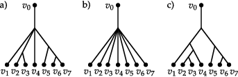
Refer to caption
Figure 5. Elements of RTree7\mathrm{RTree}_{7}

Figure 5 depicts three different examples of 77-leafed ribbon trees. Note that tree b) has no internal edges and a single internal vertex and that tree c) is a binary tree.

Let T∈RTreedT\in\mathrm{RTree}_{d} for some d∈ℕd\in\mathbb{N}. For any v∈V⁡(T)v\in V(T) let PvP_{v} denote the minimal subtree of TT which connects the root with vv, i.e. the unique subtree of TT with Ve​x​t​(Pv)={v0,v}V_{ext}(P_{v})=\left\{v_{0},v\right\}. The following statement can be shown by elementary methods of graph theory:

Lemma 3.6.

Let T∈RTreedT\in\mathrm{RTree}_{d} and e∈E⁡(T)e\in E(T). Let v,w∈V⁡(T)v,w\in V(T) be the two distinct vertices which are connected to ee. Then either v∈V⁡(Pw)v\in V\left(P_{w}\right) or w∈V⁡(Pv)w\in V\left(P_{v}\right).

Definition 3.7.

In the situation of Lemma 3.6, assume that v∈V⁡(Pw)v\in V\left(P_{w}\right). We then call vv the incoming vertex of ee and ww the outgoing vertex of ee. For any given edge ee we further denote its incoming and outgoing vertex by

vin​(e)andvout​(e).v_{\mathrm{in}}(e)\quad\text{and}\quad v_{\mathrm{out}}(e)\ .

The proof of Lemma 3.6 is elementary. Instead of providing the proof, we illustrate the situation with Figure 6 which depicts an example with d=5d=5. In the picture, the tree PvP_{v} is the subtree whose edges are the dashed edges in the picture. Here, w∈V⁡(Pv)w\in V(P_{v}).

Refer to caption
Figure 6. An illustration of Lemma 3.6.
Remark 3.8.

In this terminology, the root of a ribbon tree is always the incoming vertex of the edge it is connected to while the leaves of a ribbon tree are always the outgoing vertices of the respective edges they are connected to, i.e.

v0​(T)=vin​(e0​(T)),vi​(T)=vout​(ei​(T))∀i∈{1,…,d}.v_{0}(T)=v_{\mathrm{in}}\left(e_{0}(T)\right)\ ,\quad v_{i}(T)=v_{\mathrm{out}}\left(e_{i}(T)\right)\ \ \forall i\in\{1,\dots,d\}\ .
Lemma 3.9.

Let T∈RTreedT\in\mathrm{RTree}_{d} and v∈V⁡(T)∖{v0​(T)}v\in V(T)\setminus\{v_{0}(T)\}. There is a unique edge ev∈E⁡(T)e_{v}\in E(T) with vout​(ev)=vv_{\mathrm{out}}(e_{v})=v.

Proof.

Since v≠v0​(T)v\neq v_{0}(T), the subtree PvP_{v} has at least one edge. By definition of PvP_{v} there is an edge e∈E⁡(Pv)⊂E⁡(T)e\in E(P_{v})\subset E(T) with vout​(e)=vv_{\mathrm{out}}(e)=v.

Suppose there is an f∈E⁡(T)f\in E(T) with e≠fe\neq f and vout​(f)=vv_{\mathrm{out}}(f)=v. By definition of an outgoing vertex, this would imply that there is a minimal subtree PP of TT with

Ve​x​t​(P)={v0​(T),v}V_{ext}(P)=\{v_{0}(T),v\}

and with P≠PvP\neq P_{v}. Given PvP_{v} and PP, one could easily construct two continuous paths α1,α2:[0,1]→T\alpha_{1},\alpha_{2}:[0,1]\to T with αi​(0)=v0​(T)\alpha_{i}(0)=v_{0}(T) and αi​(1)=v\alpha_{i}(1)=v for i∈{1,2}i\in\{1,2\} and such that

im⁡α1⊂Pv,im⁡α2⊂P.\im\alpha_{1}\subset P_{v}\ ,\quad\im\alpha_{2}\subset P\ .

Via reparametrization and concatenation, one could construct a loop in TT out of α1\alpha_{1} and α2\alpha_{2} having nontrivial homotopy class. Such a loop can not exist, since TT is by definition simply connected. Therefore, the claim follows. ∎

After this graph-theoretic digression, we will focus our attention on maps T→MT\to M.

For any T∈RTreedT\in\mathrm{RTree}_{d} and e∈E⁡(T)e\in E(T) let

ae:[0,1]→Ta_{e}:[0,1]\to T

denote its attaching map. (Actually, it is an isomorphism class of attaching maps, but the meaning of this term is obvious.) We always assume that

ae​(0)=vin​(e),ae​(1)=vout​(e).a_{e}(0)=v_{\mathrm{in}}(e)\ ,\quad a_{e}(1)=v_{\mathrm{out}}(e)\ .

Via precomposing with the attaching maps, we can express every continuous map I:T→MI:T\to M as a collection of maps

{I∘ae:[0,1]→M|e∈E(T)}.\left\{I\circ a_{e}:[0,1]\to M\ |\ e\in E(T)\right\}\ .

Conversely, a family of maps

{Je:[0,1]→M|e∈E(T)}\left\{J_{e}:[0,1]\to M\ |\ e\in E(T)\right\}

induces a continuous map J:T→MJ:T\to M if and only if it satisfies the compatibility condition

(3.1) Je​(1)=Jf​(0)ifvout​(e)=vin​(f)∀e,f∈E⁡(T).J_{e}(1)=J_{f}(0)\quad\text{if}\quad v_{\mathrm{out}}(e)=v_{\mathrm{in}}(f)\qquad\forall e,f\in E(T)\ .

To apply Theorem 2.10 in this context, we want to express condition (3.1) as a certain submanifold condition for a submanifold of MNM^{N} for some N∈ℕN\in\mathbb{N}, which will lead us to the definition of TT-diagonals after some minor preparations.

For the rest of this article, we introduce the following notation for a given d∈ℕd\in\mathbb{N}:

k:RTreed→ℕ0,T↦|Ei​n​t​(T)|.k:\mathrm{RTree}_{d}\to\mathbb{N}_{0}\ ,\quad T\mapsto|E_{int}(T)|\ .

Let T∈RTreedT\in\mathrm{RTree}_{d} and consider the product manifold M1+2​k​(T)+dM^{1+2k(T)+d}. For convenience, we label its factors by the edges of TT, and write a point in M1+2​k​(T)+dM^{1+2k(T)+d} as

(q0,(qi​ne,qo​u​te)e∈Ei​n​t​(T),q1,…,qd)∈M1+2​k​(T)+d(q_{0},(q^{e}_{in},q^{e}_{out})_{e\in E_{int}(T)},q_{1},\dots,q_{d})\in M^{1+2k(T)+d}

We actually need an ordering on Ei​n​t​(T)E_{int}(T) to make this well-defined, but since the ordering is irrelevant for what follows, we silently assume that we have chosen an arbitrary ordering on Ei​n​t​(T)E_{int}(T) throughout the following discussion and leave it out of the notation.

Let w0∈V⁡(T)w_{0}\in V(T) be given by w0=vout​(e0​(T))w_{0}=v_{\mathrm{out}}(e_{0}(T)). (Recall that vin​(e0​(T))=v0​(T)v_{\mathrm{in}}(e_{0}(T))=v_{0}(T).) Define

Δw0:=\displaystyle\Delta_{w_{0}}:= {(q0,(qi​ne,qo​u​te)e∈Ei​n​t​(T),q1,…,qd)∈M1+2​k​(T)+d\displaystyle\left\{(q_{0},(q^{e}_{in},q^{e}_{out})_{e\in E_{int}(T)},q_{1},\dots,q_{d})\in M^{1+2k(T)+d}\right.
|q0=qi​ne for every e∈Ei​n​t(T) with vin(e)=w0,\displaystyle\qquad\Big|\ q_{0}=q_{in}^{e}\ \text{ for every }\ e\in E_{int}(T)\ \text{ with }\ v_{\mathrm{in}}(e)=w_{0}\ ,
q0=qj for every j∈{1,2,…,d} with vin(ej(T))=w0}.\displaystyle\qquad\qquad q_{0}=q_{j}\ \text{ for every }\ j\in\{1,2,\dots,d\}\ \text{ with }\ v_{\mathrm{in}}(e_{j}(T))=w_{0}\ \Big\}\ .

Let v∈Vi​n​t​(T)∖{w0}v\in V_{int}(T)\setminus\{w_{0}\}. By Lemma 3.9 there is a unique internal edge ev∈Ei​n​t​(T)e_{v}\in E_{int}(T) with vo​u​t​(ev)=vv_{out}(e_{v})=v. For any such vv and associated eve_{v} we define

(3.2) Δv:=\displaystyle\Delta_{v}:= {(q0,(qi​ne,qo​u​te)e∈Ei​n​t​(T),q1,…,qd)∈M1+2​k​(T)+d\displaystyle\left\{(q_{0},(q^{e}_{in},q^{e}_{out})_{e\in E_{int}(T)},q_{1},\dots,q_{d})\in M^{1+2k(T)+d}\right.
|qo​u​tev=qi​ne for every e∈Ei​n​t(T) with vin(e)=v,\displaystyle\qquad\Big|\ q_{out}^{e_{v}}=q_{in}^{e}\ \text{ for every }\ e\in E_{int}(T)\ \text{ with }\ v_{\mathrm{in}}(e)=v\ ,
qo​u​tev=qj for every j∈{1,…,d} with vin(ej(T))=v}.\displaystyle\qquad\qquad q_{out}^{e_{v}}=q_{j}\ \text{ for every }\ j\in\{1,\dots,d\}\ \text{ with }\ v_{\mathrm{in}}(e_{j}(T))=v\ \Big\}\ .
Definition 3.10.

The TT-diagonal ΔT⊂M1+2​k​(T)+d\Delta_{T}\subset M^{1+2k(T)+d} is the space given by

ΔT:=⋂v∈Vi​n​t​(T)Δv.\Delta_{T}:=\bigcap_{v\in V_{int}(T)}\Delta_{v}\ .

The definition of ΔT\Delta_{T} will be motivated in Remark 3.12.

Proposition 3.11.

For every T∈RTreedT\in\mathrm{RTree}_{d} with d≥2d\geq 2, the TT-diagonal is a submanifold of M1+2​k​(T)+dM^{1+2k(T)+d} with

(3.3) codim⁡ΔT=(k⁡(T)+d)⋅n.\codim\Delta_{T}=(k(T)+d)\cdot n\ .
Proof.

For every v∈Vi​n​t​(T)v\in V_{int}(T), the space Δv\Delta_{v} is easily seen to be a submanifold of M1+2​k​(T)+dM^{1+2k(T)+d} with

codim⁡Δv=|{e∈E⁡(T)|vin​(e)=v}|⋅n.\codim\Delta_{v}=\left|\{e\in E(T)\ |\ v_{\mathrm{in}}(e)=v\}\right|\cdot n\ .

Furthermore, for every V⊂Vi​n​t​(T)V\subset V_{int}(T) and v0∈Vi​n​t​(T)v_{0}\in V_{int}(T) with v0∉Vv_{0}\notin V, the spaces Δv0\Delta_{v_{0}} and ⋂v∈VΔv\bigcap_{v\in V}\Delta_{v} are smooth submanifolds and transverse to each other. Then one can build up the space ΔT\Delta_{T} as a finite sequence of transverse intersections of submanifolds and derive that it is itself a smooth submanifold, whose codimension is given by

codim⁡ΔT\displaystyle\codim\Delta_{T} =∑v∈Vi​n​t​(T)codim⁡Δv=∑v∈Vi​n​t​(T)|{e∈E⁡(T)|vin​(e)=v}|⋅n\displaystyle=\sum_{v\in V_{int}(T)}\codim\Delta_{v}=\sum_{v\in V_{int}(T)}\left|\{e\in E(T)\ |\ v_{\mathrm{in}}(e)=v\}\right|\cdot n
=|{e∈E⁡(T)|vin​(e)∈Vi​n​t​(T)}|⋅n.\displaystyle=\left|\{e\in E(T)\ |\ v_{\mathrm{in}}(e)\in V_{int}(T)\}\right|\cdot n\ .

All that remains to do is to determine the cardinality of {e∈E⁡(T)|vin​(e)∈Vi​n​t​(T)}\{e\in E(T)\ |\ v_{\mathrm{in}}(e)\in V_{int}(T)\}. By definition of e0​(T)e_{0}(T) we know that vin​(e0​(T))=v0∉Vi​n​t​(T)v_{\mathrm{in}}(e_{0}(T))=v_{0}\notin V_{int}(T), such that e0​(T)e_{0}(T) does not lie in this set. But e0​(T)e_{0}(T) is the only edge not lying in this set. The incoming vertex of an internal edge is by definition internal. Moreover, for all external edges ee with e≠e0e\neq e_{0} it holds that

vout​(e)∈{v1​(T),…,vd​(T)}⊂Ve​x​t​(T),v_{\mathrm{out}}(e)\in\{v_{1}(T),\dots,v_{d}(T)\}\subset V_{ext}(T)\ ,

so the incoming vertex of ee has to be internal since d≥2d\geq 2. Consequently, we obtain

codim⁡ΔT=|(E⁡(T)∖{e0​(T)})|⋅n=(k⁡(T)+d)⋅n.\codim\Delta_{T}=\left|(E(T)\setminus\{e_{0}(T)\})\right|\cdot n=(k(T)+d)\cdot n\ .

∎

Remark 3.12.

Combining the conditions in the definitions of the different Δv\Delta_{v}, v∈Vi​n​t​(T)v\in V_{int}(T), one derives that the TT-diagonal is explicitly described by

ΔT:=\displaystyle\Delta_{T}:= {(q0,(qine,qoute)e∈Ei​n​t​(T),q1,…,qd)∈M1+2​k​(T)+d\displaystyle\left\{(q_{0},(q^{e}_{\mathrm{in}},q^{e}_{\mathrm{out}})_{e\in E_{int}(T)},q_{1},\dots,q_{d})\in M^{1+2k(T)+d}\right.
|qoute=qinf for all e,f∈Ei​n​t(T) with vout(e)=vin(f),\displaystyle\quad\left|\ q_{\mathrm{out}}^{e}=q_{\mathrm{in}}^{f}\ \text{ for all }\ e,f\in E_{int}(T)\ \text{ with }\ v_{\mathrm{out}}(e)=v_{\mathrm{in}}(f)\ ,\right.
qoute=qj​ for every ​e∈Ei​n​t​(T),j∈{1,2,…,d}​ with ​vout​(e)=vin​(ej​(T)),\displaystyle\quad\ \ q_{\mathrm{out}}^{e}=q_{j}\ \text{ for every }\ e\in E_{int}(T),\ j\in\{1,2,\dots,d\}\ \text{ with }\ v_{\mathrm{out}}(e)=v_{\mathrm{in}}(e_{j}(T))\ ,
q0=qine for every e∈Ei​n​t(T) with vout(e0(T))=vin(e)}.\displaystyle\quad\left.\ q_{0}=q_{\mathrm{in}}^{e}\ \text{ for every }\ e\in E_{int}(T)\ \text{ with }\ v_{\mathrm{out}}(e_{0}(T))=v_{\mathrm{in}}(e)\ \right\}\ .

Let {Je:[0,1]→M|e∈E(T)}\{J_{e}:[0,1]\to M\ |e\in E(T)\} be a family of maps. If one writes down condition (3.1) in greater detail for the different types of edges, one will obtain that the family induces a continuous map T→MT\to M if and only if

(Je0​(1),(Je​(0),Je​(1))e∈Ei​n​t​(T),Je1​(0),…,Jed​(0))∈ΔT,\left(J_{e_{0}}(1),\left(J_{e}(0),J_{e}(1)\right)_{e\in E_{int}(T)},J_{e_{1}}(0),\dots,J_{e_{d}}(0)\right)\in\Delta_{T}\ ,

where ei:=ei​(T)e_{i}:=e_{i}(T) for every i∈{0,1,…,d}i\in\{0,1,\dots,d\}. In other words, we have expressed condition (3.1) in terms of the TT-diagonal.

After all these preparations, we build the bridge to the Morse-theoretic constructions from Sections 1 and 2. We want to consider maps from ribbon trees to MM which are not only continuous, but whose attaching maps fulfill (up to reparametrization) a perturbed negative gradient flow equation. Similar as in Remark 3.12, we will piece these maps together out of a family of maps indexed by the set of edges of the ribbon tree.

We start with describing suitable perturbation spaces. Let d≥2d\geq 2 and T∈RTreedT\in\mathrm{RTree}_{d} be fixed.

Definition 3.13.

We introduce the space of perturbations for TT as

𝔛⁡(T):=𝔛⁡(1,k⁡(T),d),\mathfrak{X}(T):=\mathfrak{X}(1,k(T),d)\ ,

In the case that k⁡(T)>0k(T)>0, we further consider the space of background perturbations for TT

𝔛back​(T):=𝔛back​(1,k⁡(T),d),\mathfrak{X}^{\text{back}}(T):=\mathfrak{X}^{\text{back}}(1,k(T),d)\ ,

using the notation of Section 2. For 𝐗∈𝔛back​(T)\mathbf{X}\in\mathfrak{X}^{\text{back}}(T), the space of perturbations for TT with background perturbation 𝐗\mathbf{X} is defined by

𝔛⁡(T,𝐗):=𝔛⁡(1,k⁡(T),d,𝐗),\mathfrak{X}(T,\mathbf{X}):=\mathfrak{X}(1,k(T),d,\mathbf{X})\ ,

once more using the notation of Section 2.

We are again silently assuming that an ordering of Ei​n​t​(T)E_{int}(T) has been chosen and keep it out of the notation. We therefore write perturbations 𝐘∈𝔛⁡(T)\mathbf{Y}\in\mathfrak{X}(T) as

𝐘=(Y0,(Ye)e∈Ei​n​t​(T),Y1,…,Yd),\mathbf{Y}=(Y_{0},(Y_{e})_{e\in E_{int}(T)},Y_{1},\dots,Y_{d})\ ,

where Y0∈𝔛−​(M,k⁡(T))Y_{0}\in\mathfrak{X}_{-}(M,k(T)), Ye∈𝔛0​(M,k⁡(T)−1)Y_{e}\in\mathfrak{X}_{0}(M,k(T)-1) for all e∈Ei​n​t​(T)e\in E_{int}(T) and Yi∈𝔛+​(M,k⁡(T))Y_{i}\in\mathfrak{X}_{+}(M,k(T)) for all i∈{1,2,…,d}i\in\{1,2,\dots,d\}. In strict analogy with the notation from Definition 2.9, we further write 𝐗∈𝔛back​(T)\mathbf{X}\in\mathfrak{X}^{\text{back}}(T) as

𝐗=(𝐗−,(𝐗e0)e∈Ei​n​t​(T),𝐗1+,…,𝐗d+),\mathbf{X}=\Bigl(\mathbf{X}^{-},\left(\mathbf{X}^{0}_{e}\right)_{e\in E_{int}(T)},\mathbf{X}^{+}_{1},\dots,\mathbf{X}^{+}_{d}\Big)\ ,

where

  • •

    𝐗−∈𝔛−back​(M,k⁡(T))\mathbf{X}^{-}\in\mathfrak{X}^{\text{back}}_{-}(M,k(T)) is written as 𝐗−=(Xe−)e∈Ei​n​t​(T)\mathbf{X}^{-}=\left(X^{-}_{e}\right)_{e\in E_{int}(T)} ,

  • •

    𝐗e0∈𝔛0back​(M,k⁡(T)−1)\mathbf{X}^{0}_{e}\in\mathfrak{X}^{\text{back}}_{0}(M,k(T)-1) is denoted by

    𝐗e0=((Xe​f0)f∈Ei​n​t​(T)∖{e},Xe+,Xe−)for every​e∈Ei​n​t​(T),\mathbf{X}^{0}_{e}=\Big(\left(X^{0}_{ef}\right)_{f\in E_{int}(T)\setminus\{e\}},X_{e+},X_{e-}\Big)\quad\text{for every}\ e\in E_{int}(T)\ ,
  • •

    𝐗i+∈𝔛+back​(M,k⁡(T))\mathbf{X}^{+}_{i}\in\mathfrak{X}^{\text{back}}_{+}(M,k(T)) is given by

    𝐗i+=(Xe+)e∈Ei​n​t​(T)for every​i∈{1,2,…,d}.\mathbf{X}^{+}_{i}=\left(X^{+}_{e}\right)_{e\in E_{int}(T)}\quad\text{for every}\ i\in\{1,2,\dots,d\}\ .

Note that if 𝐘∈𝔛⁡(T,𝐗)\mathbf{Y}\in\mathfrak{X}(T,\mathbf{X}), then the above notation implies that

Y0∈𝔛−(M,k(T),𝐗−),Ye∈𝔛0(M,k(T),𝐗e0)andYi∈𝔛+(M,k(T),𝐗i+)Y_{0}\in\mathfrak{X}_{-}(M,k(T),\mathbf{X}^{-})\ ,\quad Y_{e}\in\mathfrak{X}_{0}(M,k(T),\mathbf{X}^{0}_{e})\ \ \text{and}\ \ Y_{i}\in\mathfrak{X}_{+}(M,k(T),\mathbf{X}^{+}_{i})

for every e∈Ei​n​t​(T)e\in E_{int}(T) and i∈{1,…,d}i\in\{1,\dots,d\}.

Definition 3.14.

Let 𝐗∈𝔛back​(T)\mathbf{X}\in\mathfrak{X}^{\text{back}}(T) and 𝐘∈𝔛⁡(T,𝐗)\mathbf{Y}\in\mathfrak{X}(T,\mathbf{X}) and x0,x1,…,xd∈Crit ⁡fx_{0},x_{1},\dots,x_{d}\in\Crit f. The moduli space of 𝐘\mathbf{Y}-perturbed Morse ribbon trees modelled on TT starting in x0x_{0} and ending in x1,…,xdx_{1},\dots,x_{d} is defined as

𝒜𝐘d​(x0,x1,…,xd,T)\displaystyle\mathcal{A}^{d}_{\mathbf{Y}}(x_{0},x_{1},\dots,x_{d},T)
:={(γ0,(le,γe)e∈Ei​n​t​(T),γ1,…,γd)|γ0∈𝒫−(x0),γi∈𝒫+(xi)∀i∈{1,2,…,d},\displaystyle:=\left\{\left.\left(\gamma_{0},\left(l_{e},\gamma_{e}\right)_{e\in E_{int}(T)},\gamma_{1},\dots,\gamma_{d}\right)\ \right|\ \gamma_{0}\in\mathcal{P}_{-}(x_{0}),\ \gamma_{i}\in\mathcal{P}_{+}(x_{i})\ \forall i\in\{1,2,\dots,d\}\ ,\right.
le>0,γe∈H1​([0,le],M)​∀e∈Ei​n​t​(T),\displaystyle\quad l_{e}>0,\ \gamma_{e}\in H^{1}([0,l_{e}],M)\ \forall e\in E_{int}(T)\ ,
γ˙0(s)+(∇f)(γ0(s))+Y0((le)e∈Ei​n​t​(T),s,γ0(s))=0∀s∈(−∞,0],\displaystyle\quad\dot{\gamma}_{0}(s)+(\nabla f)(\gamma_{0}(s))+Y_{0}\left(\left(l_{e}\right)_{e\in E_{int}(T)},s,\gamma_{0}(s)\right)=0\quad\forall s\in(-\infty,0]\ ,
γ˙i(s)+(∇f)(γi(s))+Yi((le)e∈Ei​n​t​(T),s,γi(s))=0∀s∈[0,+∞)∀i∈{1,…,d},\displaystyle\quad\dot{\gamma}_{i}(s)+(\nabla f)(\gamma_{i}(s))+Y_{i}\left(\left(l_{e}\right)_{e\in E_{int}(T)},s,\gamma_{i}(s)\right)=0\quad\forall s\in[0,+\infty)\ \forall i\in\{1,\dots,d\}\ ,
γ˙e​(s)+(∇f)​(γe​(s))+Ye​((lf)f∈Ei​n​t​(T)∖{e},le,s,γe​(s))=0∀s∈[0,le]​∀e∈Ei​n​t​(T),\displaystyle\quad\dot{\gamma}_{e}(s)+(\nabla f)(\gamma_{e}(s))+Y_{e}\left(\left(l_{f}\right)_{f\in E_{int}(T)\setminus\{e\}},l_{e},s,\gamma_{e}(s)\right)=0\quad\forall s\in[0,l_{e}]\ \forall e\in E_{int}(T)\ ,
γe​(le)=γf​(0)​ for all ​e,f∈Ei​n​t​(T)​ with ​vout​(e)=vin​(f),\displaystyle\quad\gamma_{e}(l_{e})=\gamma_{f}(0)\ \text{ for all }\ e,f\in E_{int}(T)\ \text{ with }\ v_{\mathrm{out}}(e)=v_{\mathrm{in}}(f)\ ,
γe​(le)=γj​(0)​ for all ​e∈Ei​n​t​(T),j∈{1,2,…,d}​ with ​vout​(e)=vin​(ej​(T)),\displaystyle\quad\gamma_{e}(l_{e})=\gamma_{j}(0)\ \text{ for all }\ e\in E_{int}(T),\ j\in\{1,2,\dots,d\}\ \text{ with }\ v_{\mathrm{out}}(e)=v_{\mathrm{in}}(e_{j}(T))\ ,
γ0(0)=γe(0) for all e∈Ei​n​t(T) with vout(e0(T))=vin(e)}.\displaystyle\quad\gamma_{0}(0)=\gamma_{e}(0)\ \text{ for all }\ e\in E_{int}(T)\ \text{ with }\ v_{\mathrm{out}}(e_{0}(T))=v_{\mathrm{in}}(e)\ \Big\}\ .
Refer to caption
Figure 7. An element of 𝒜𝐘d​(x0,x1,…,xd,T)\mathcal{A}^{d}_{\mathbf{Y}}(x_{0},x_{1},\dots,x_{d},T).

See Figure 7 for a picture of a perturbed Morse ribbon tree. The conditions in the last three lines of the definition of 𝒜𝐘d​(x0,x1,…,xd,T)\mathcal{A}^{d}_{\mathbf{Y}}(x_{0},x_{1},\dots,x_{d},T) can be loosely rephrased by saying that all the trajectories associated to the edges of TT are coupled at the common associated vertices. They ensure that the family of trajectories induces a continuous map T→MT\to M.

The proof of the following theorem is a major application of the results of Section 2 and especially of Theorem 2.10.

Theorem 3.15.

Let 𝐗∈𝔛back​(T)\mathbf{X}\in\mathfrak{X}^{\text{back}}(T). For generic choice of 𝐘∈𝔛⁡(T,𝐗)\mathbf{Y}\in\mathfrak{X}(T,\mathbf{X}), the moduli space 𝒜𝐘d​(x0,x1,…,xd,T)\mathcal{A}^{d}_{\mathbf{Y}}(x_{0},x_{1},\dots,x_{d},T) can be equipped with the structure of a manifold of class Cn+1C^{n+1} of dimension

dim𝒜𝐘d​(x0,x1,…,xd,T)=μ⁡(x0)−∑j=1dμ⁡(xj)+k⁡(T)\dim\mathcal{A}^{d}_{\mathbf{Y}}(x_{0},x_{1},\dots,x_{d},T)=\mu(x_{0})-\sum_{j=1}^{d}\mu(x_{j})+k(T)

for all x0,x1,…,xd∈Crit ⁡fx_{0},x_{1},\dots,x_{d}\in\Crit f.

Proof.

In strict analogy with Remark 3.12, the endpoint conditions, i.e. the last three lines in the definition of 𝒜𝐘d​(x0,x1,…,xd,T)\mathcal{A}^{d}_{\mathbf{Y}}(x_{0},x_{1},\dots,x_{d},T), are equivalent to

(γ0​(0),(γe​(0),γe​(le))e∈Ei​n​t​(T),γ1​(0),…,γd​(0))∈ΔT.\left(\gamma_{0}(0),\left(\gamma_{e}(0),\gamma_{e}(l_{e})\right)_{e\in E_{int}(T)},\gamma_{1}(0),\dots,\gamma_{d}(0)\right)\in\Delta_{T}\ .

Using the notation of Section 2, this condition can be reformulated as

E¯𝐘​(γ0,(le,γe)e∈Ei​n​t​(T),γ1,…,γd)∈ΔT,\underline{E}_{\mathbf{Y}}\left(\gamma_{0},\left(l_{e},\gamma_{e}\right)_{e\in E_{int}(T)},\gamma_{1},\dots,\gamma_{d}\right)\in\Delta_{T}\ ,

where E¯𝐘\underline{E}_{\mathbf{Y}} is defined as the corresponding product of evaluation maps as in the definition of the moduli space in Theorem 2.10.

This reformulation implies that in the notation of Theorem 2.10 the following equality holds true:

𝒜𝐘d​(x0,x1,…,xd,T)=ℳ𝐘​(x0,(x1,…,xd),(1,k⁡(T),d),(0,+∞)k⁡(T),ΔT).\mathcal{A}^{d}_{\mathbf{Y}}(x_{0},x_{1},\dots,x_{d},T)=\mathcal{M}_{\mathbf{Y}}\left(x_{0},(x_{1},\dots,x_{d}),(1,k(T),d),\left(0,+\infty\right)^{k(T)},\Delta_{T}\right)\ .

Thus, the statement is nothing but a straightforward consequence of Theorem 2.10. It remains to show that the claimed dimension formula coincides with the one from Theorem 2.10. The latter one yields:

dim𝒜𝐘d​(x0,x1,…,xd,T,𝐗)\displaystyle\dim\mathcal{A}^{d}_{\mathbf{Y}}(x_{0},x_{1},\dots,x_{d},T,\mathbf{X}) =μ⁡(x0)−∑i=1dμ⁡(xi)+(k⁡(T)+d)​n+k⁡(T)−codim⁡ΔT\displaystyle=\mu(x_{0})-\sum_{i=1}^{d}\mu(x_{i})+(k(T)+d)n+k(T)-\codim\Delta_{T}
=μ⁡(x0)−∑i=1dμ⁡(xi)+k⁡(T),\displaystyle=\mu(x_{0})-\sum_{i=1}^{d}\mu(x_{i})+k(T)\ ,

where the second equality is a consequence of Proposition 3.11. ∎

Definition 3.16.

A perturbation 𝐘∈𝔛⁡(T)\mathbf{Y}\in\mathfrak{X}(T) for which 𝒜𝐘d​(x0,x1,…,xd,T,𝐗)\mathcal{A}^{d}_{\mathbf{Y}}(x_{0},x_{1},\dots,x_{d},T,\mathbf{X}) can be equipped with the structure of a manifold of class Cn+1C^{n+1} for all x0,x1,…,xd∈Crit ⁡fx_{0},x_{1},\dots,x_{d}\in\Crit f is called regular.

4. The convergence behaviour of sequences of perturbed Morse ribbon trees

After having constructed moduli spaces of perturbed Morse ribbon trees in the previous section, we want to investigate sequential compactness properties of these moduli spaces. Our starting point is the consideration of certain sequential compactness results for spaces of perturbed Morse trajectories of the three different types we introduced in Section 1. We will show that in all three cases, every sequence in the respective moduli space without a convergent subsequence has a subsequence that converges geometrically against a family of trajectories. The notion of geometric convergence will be made precise in the course of this section.

Afterwards, we will draw conclustions from these results for spaces of perturbed Morse ribbon trees. The main result of this section is Theorem 4.10, following immediately from the results for perturbed Morse trajectories. It roughly states that every sequence of perturbed Morse ribbon trees without a subsequence which converges in its respective domain, has a geometrically convergent subsequence. This notion of geometric convergence will be defined later.

Having established the main compactness result, we will focus our attention on certain special cases. Theorems 4.15, 4.16 and 4.17 describe possibilites for the limiting behaviour of sequences of perturbed Morse ribbon trees in greater detail.

Finally, we formulate a theorem for describing the situation of simultaneous occurence of the convergence phenomena described in the aforementioned three theorems. This theorem will enable us to investigate the spaces of geometric limits of sequences of perturbed Morse ribbon trees. Eventually, we will use the structure of the limit spaces to construct higher order multiplications on Morse cochain complexes in Section 5.

The sequential compactness theorems for moduli spaces of perturbed Morse trajectories can be shown in strict analogy with the compactness results in the unperturbed case. The compactness result for semi-infinite Morse trajectories is shown in [Sch99, Section 4], while the compactness result for finite-length Morse trajectories is proven in [Weh12], along with a more general statement covering the semi-infinite case as well.

The line of argument of the respective reference can be transferred to the case of perturbed Morse trajectories with only minor changes. Therefore, we will omit parts of the proofs of the decisive compactness theorems in this section and apply the respective trajectory compactness theorem instead.

Throughout this section, we assume that every ribbon tree is equipped with an ordering of its internal edges. All results of this section are independent of the chosen orderings. We will come back to these choices in Section 5 and Appendix A.

We begin this section by stating the crucial sequential compactness theorem for perturbed semi-infinite Morse trajectories. For every x,y∈Crit ⁡fx,y\in\Crit f let

ℳ^​(x,y):=ℳ^​(x,y,g)\widehat{\mathcal{M}}(x,y):=\widehat{\mathcal{M}}(x,y,g)

denote the space of unparametrized negative gradient flow lines of ff with respect to gg, as defined in the introduction of this article.

Theorem 4.1.
  1. (i)

    Let x∈Crit ⁡fx\in\Crit f, {γn}n∈ℕ⊂𝒫−​(x)\{\gamma_{n}\}_{n\in\mathbb{N}}\subset\mathcal{P}_{-}(x), Y∞∈𝔛−​(M)Y_{\infty}\in\mathfrak{X}_{-}(M) and {Yn}n∈ℕ\{Y_{n}\}_{n\in\mathbb{N}} be a sequence in 𝔛−​(M)\mathfrak{X}_{-}(M) which converges against Y∞Y_{\infty} and such that

    γn∈W−​(x,Yn)for everyn∈ℕ.\gamma_{n}\in W^{-}\left(x,Y_{n}\right)\quad\text{for every}\ \ n\in\mathbb{N}\ .

    If {γn}n∈ℕ\{\gamma_{n}\}_{n\in\mathbb{N}} does not have a subsequence which converges in 𝒫−​(x)\mathcal{P}_{-}(x), then there will be m∈ℕm\in\mathbb{N}, x1,…,xm∈Crit ⁡fx_{1},\dots,x_{m}\in\Crit f with μ⁡(x)>μ⁡(x1)>⋯>μ⁡(xm)\mu(x)>\mu(x_{1})>\dots>\mu(x_{m}) and curves

    (g^1,…,g^m,γ−)∈ℳ^​(x,x1)×ℳ^​(x1,x2)×⋯×ℳ^​(xm−1,xm)×W−​(xm,Y∞),(\hat{g}_{1},\dots,\hat{g}_{m},\gamma_{-})\in\widehat{\mathcal{M}}(x,x_{1})\times\widehat{\mathcal{M}}(x_{1},x_{2})\times\dots\times\widehat{\mathcal{M}}(x_{m-1},x_{m})\times W^{-}\left(x_{m},Y_{\infty}\right)\ ,

    as well as a sequence {τqj}q∈ℕ⊂ℝ\{\tau^{j}_{q}\}_{q\in\mathbb{N}}\subset\mathbb{R} diverging to −∞-\infty for every j∈{1,2,…,m}j\in\{1,2,\dots,m\} and a subsequence {γnq}q∈ℕ\{\gamma_{n_{q}}\}_{q\in\mathbb{N}} such that

    • •

      {γnq}q∈ℕ\{\gamma_{n_{q}}\}_{q\in\mathbb{N}} converges against γ−\gamma_{-} in the Cl​o​c∞C^{\infty}_{loc}-topology,

    • •

      {γnq(⋅+τqj)|(−∞,T]}q≥qT,j\Bigl\{\left.\gamma_{n_{q}}\left(\cdot+\tau^{j}_{q}\right)\right|_{(-\infty,T]}\Bigr\}_{q\geq q_{T,j}} converges against gj|(−∞,T]g_{j}|_{(-\infty,T]} in the Cl​o​c∞C^{\infty}_{loc}-topology for all T>0T>0 and qT,j∈ℕq_{T,j}\in\mathbb{N} for which the restrictions are well-defined, where gjg_{j} is a representative of g^j\hat{g}_{j} for every j∈{1,2,…,m}j\in\{1,2,\dots,m\}.

  2. (ii)

    Let y∈Crit ⁡fy\in\Crit f, {γn}n∈ℕ⊂𝒫+​(y)\{\gamma_{n}\}_{n\in\mathbb{N}}\subset\mathcal{P}^{+}(y), {Yn}n∈ℕ⊂𝔛+​(M)\{Y_{n}\}_{n\in\mathbb{N}}\subset\mathfrak{X}_{+}(M) and Y∞∈𝔛+​(M)Y_{\infty}\in\mathfrak{X}_{+}(M) such that {Yn}n∈ℕ\{Y_{n}\}_{n\in\mathbb{N}} converges against Y∞Y_{\infty} and

    γn∈W+​(x,Yn)for everyn∈ℕ.\gamma_{n}\in W^{+}\left(x,Y_{n}\right)\quad\text{for every}\ \ n\in\mathbb{N}\ .

    If {γn}n∈ℕ\{\gamma_{n}\}_{n\in\mathbb{N}} does not have a subsequence which converges in 𝒫+​(y)\mathcal{P}_{+}(y), then there will be m∈ℕm\in\mathbb{N}, y1,…,ym∈Crit ⁡fy_{1},\dots,y_{m}\in\Crit f with μ⁡(y1)>⋯>μ⁡(ym)>μ⁡(y)\mu(y_{1})>\dots>\mu(y_{m})>\mu(y) and curves

    (γ+,g^1,…,g^m)∈W+​(y1,Y∞)×ℳ^​(y1,y2)×⋯×ℳ^​(ym−1,ym)×ℳ^​(ym,y),(\gamma_{+},\hat{g}_{1},\dots,\hat{g}_{m})\in W^{+}\left(y_{1},Y_{\infty}\right)\times\widehat{\mathcal{M}}(y_{1},y_{2})\times\dots\times\widehat{\mathcal{M}}(y_{m-1},y_{m})\times\widehat{\mathcal{M}}(y_{m},y)\ ,

    as well a sequence {τqj}q∈ℕ⊂ℝ\{\tau^{j}_{q}\}_{q\in\mathbb{N}}\subset\mathbb{R} diverging to +∞+\infty for every j∈{1,…,m}j\in\{1,\dots,m\} and a subsequence {γnq}q∈ℕ\{\gamma_{n_{q}}\}_{q\in\mathbb{N}} such that

    • •

      {γnq}q∈ℕ\{\gamma_{n_{q}}\}_{q\in\mathbb{N}} converges against γ+\gamma_{+} in the Cl​o​c∞C^{\infty}_{loc}-topology,

    • •

      {γnq(⋅+τqj)|[−T,+∞)}q≥qT,j\Bigl\{\left.\gamma_{n_{q}}\left(\cdot+\tau^{j}_{q}\right)\right|_{[-T,+\infty)}\Bigr\}_{q\geq q_{T,j}} converges against gj|[−T,+∞)g_{j}|_{[-T,+\infty)} in the Cl​o​c∞C^{\infty}_{loc}-topology for every T>0T>0 and every qn,T∈ℕq_{n,T}\in\mathbb{N} such that the restrictions are well-defined, for a representative gjg_{j} of g^j\hat{g}_{j} for every j∈{1,2,…,m}j\in\{1,2,\dots,m\}.

Theorem 4.1 is shown by applying the methods used to prove the corresponding result for unperturbed half-trajectories. For compactness theorems for spaces of unperturbed Morse trajectories, see [Weh12, Theorem 2.6] or [Sch93, Section 2.4] for analogous results for trajectories defined on ℝ\mathbb{R}.

Refer to caption
Figure 8. A geometrically convergent sequence of perturbed semi-infinite half-trajectories ending in y∈Crit ⁡fy\in\Crit f.

Figure 8 illustrates part (ii) of Theorem 4.1. For an illustration of part (i), turn Figure 8 upside down and invert the directions of all arrows.

Remark 4.2.

Concerning Theorem 4.1, it is of great importance that the spaces 𝔛±​(M)\mathfrak{X}_{\pm}(M) are defined such that for every Y∈𝔛±​(M)Y\in\mathfrak{X}_{\pm}(M), the value Y⁡(t,x)Y\left(t,x\right) vanishes whenever tt lies below the fixed value −1-1 and above the fixed value 11 in the positive case.

If the perturbations were allowed to be non-vanishing for arbitrary time parameters, the sequences of reparametrization times {τnj}n∈ℕ\{\tau^{j}_{n}\}_{n\in\mathbb{N}} would in general not exist in the above setting.

Definition 4.3.
  1. (i)

    In the situation of Theorem 4.1 (i), we say that {γn}n∈ℕ\{\gamma_{n}\}_{n\in\mathbb{N}} converges geometrically against (g^1,…,g^m,γ−)(\hat{g}_{1},\dots,\hat{g}_{m},\gamma_{-}) and we call (g^1,…,g^m,γ−)(\hat{g}_{1},\dots,\hat{g}_{m},\gamma_{-}) the geometric limit of {γn}n∈ℕ\left\{\gamma_{n}\right\}_{n\in\mathbb{N}}.

  2. (ii)

    In the situation of Theorem 4.1 (ii), we say that {γn}n∈ℕ\{\gamma_{n}\}_{n\in\mathbb{N}} converges geometrically against (γ+,g^1,…,g^m)(\gamma_{+},\hat{g}_{1},\dots,\hat{g}_{m}) and we call (γ+,g^1,…,g^m)(\gamma_{+},\hat{g}_{1},\dots,\hat{g}_{m}) the geometric limit of {γn}n∈ℕ\left\{\gamma_{n}\right\}_{n\in\mathbb{N}}.

Remark 4.4.

The following special case of Theorem 4.1 will be relevant in the discussion of the convergence of perturbed Morse ribbon trees. Let Y∈𝔛−​(M,k,𝐗)Y\in\mathfrak{X}_{-}(M,k,\mathbf{X}) for a given background perturbation 𝐗=(X1,…,Xk)∈𝔛−back​(M,k)\mathbf{X}=(X_{1},\dots,X_{k})\in\mathfrak{X}^{\text{back}}_{-}(M,k). Let {(l1​n,…,lk​n)}n∈ℕ\{(l_{1n},\dots,l_{kn})\}_{n\in\mathbb{N}} be a sequence in (0,+∞)k(0,+\infty)^{k}, such that {li​n}n∈ℕ\{l_{in}\}_{n\in\mathbb{N}} diverges against +∞+\infty for a unique i∈{1,2,…,k}i\in\{1,2,\dots,k\} and that {lj​n}n∈ℕ\{l_{jn}\}_{n\in\mathbb{N}} converges against lj​∞∈[0,+∞)l_{j\infty}\in[0,+\infty) if j≠ij\neq i. Define Yn∈𝔛−​(M)Y_{n}\in\mathfrak{X}_{-}(M) for every n∈ℕn\in\mathbb{N} by

Yn(t,x):=Y((l1​n,…,lk​n),t,x)∀t∈(−∞,0],x∈M,Y_{n}(t,x):=Y\left((l_{1n},\dots,l_{kn}),t,x\right)\quad\forall t\in(-\infty,0]\ ,\ \ x\in M\ ,

let x∈Crit ⁡fx\in\Crit f and let {γn}n∈ℕ\{\gamma_{n}\}_{n\in\mathbb{N}} be a sequence with γn∈W−​(x,Yn)\gamma_{n}\in W^{-}(x,Y_{n}) for every n∈ℕn\in\mathbb{N}. If {γn}n∈ℕ\{\gamma_{n}\}_{n\in\mathbb{N}} converges geometrically in this situation, then it will hold for the geometric limit (g^1,…,g^m,γ−)(\hat{g}_{1},\dots,\hat{g}_{m},\gamma_{-}) by definition of a background perturbation that

γ−∈W−​(xm,Xi​(l1​∞,…,l(i−1)​∞,l(i+1)​∞,…,lk​∞)).\gamma_{-}\in W^{-}(x_{m},X_{i}(l_{1\infty},\dots,l_{(i-1)\infty},l_{(i+1)\infty},\dots,l_{k\infty}))\ .

The analogous remark is true for positive semi-infinite half-trajectories.

The convergence theorem for perturbed finite-length Morse trajectories takes a similar form, but we need to introduce the right notion of convergence in advance.

Definition 4.5.

Let {Yn}n∈ℕ⊂𝔛0​(M)\{Y_{n}\}_{n\in\mathbb{N}}\subset\mathfrak{X}_{0}(M) be a sequence converging against Y∞∈𝔛0​(M)Y_{\infty}\in\mathfrak{X}_{0}(M) and let {(ln,γn)}n∈ℕ\left\{(l_{n},\gamma_{n})\right\}_{n\in\mathbb{N}} be a sequence with ln≥0l_{n}\geq 0, γn:[0,ln]→M\gamma_{n}:[0,l_{n}]\to M and (ln,γn)∈ℳ⁡(Yn)(l_{n},\gamma_{n})\in\mathcal{M}\left(Y_{n}\right) for all n∈ℕn\in\mathbb{N}. The sequence {(ln,γn)}n∈ℕ\left\{(l_{n},\gamma_{n})\right\}_{n\in\mathbb{N}} is called convergent iff the sequence {ψYn​(ln,γn)}n∈ℕ\left\{\psi_{Y_{n}}(l_{n},\gamma_{n})\right\}_{n\in\mathbb{N}} converges in ℳ⁡(f,g)\mathcal{M}(f,g). Here, we use the map ψ\psi from (1.15) and put ψYn:=ψ⁡(Yn,⋅)\psi_{Y_{n}}:=\psi\left(Y_{n},\cdot\right) for every n∈ℕn\in\mathbb{N}. Every such

ψYn:ℳ⁡(Yn)→≅ℳ⁡(f,g)\psi_{Y_{n}}:\mathcal{M}\left(Y_{n}\right)\stackrel{{\scriptstyle\cong}}{{\to}}\mathcal{M}(f,g)

is a diffeomorphism of class Cn+1C^{n+1}.

Theorem 4.6.

Let k∈ℕ0k\in\mathbb{N}_{0} and let {Yn}n∈ℕ⊂𝔛0​(M)\{Y_{n}\}_{n\in\mathbb{N}}\subset\mathfrak{X}_{0}(M) be a sequence converging against some Y∞∈𝔛0​(M)Y_{\infty}\in\mathfrak{X}_{0}(M). Consider a sequence {(ln,γn)}n∈ℕ\{(l_{n},\gamma_{n})\}_{n\in\mathbb{N}} with (ln,γn)∈ℳ⁡(Yn)(l_{n},\gamma_{n})\in\mathcal{M}\left(Y_{n}\right) for every n∈ℕn\in\mathbb{N}. If the sequence {(ln,γn)}n∈ℕ\{(l_{n},\gamma_{n})\}_{n\in\mathbb{N}} does not have a convergent subsequence, then there are a subsequence {(lnq,γnq)}q∈ℕ\{(l_{n_{q}},\gamma_{n_{q}})\}_{q\in\mathbb{N}} with

limq→∞lnq=+∞,\lim_{q\to\infty}l_{n_{q}}=+\infty\ ,

m∈ℕm\in\mathbb{N}, x1,…,xm∈Crit ⁡fx_{1},\dots,x_{m}\in\Crit f, {sqj}q∈ℕ⊂ℝ\{s^{j}_{q}\}_{q\in\mathbb{N}}\subset\mathbb{R} for every j∈{1,…,m−1}j\in\{1,\dots,m-1\} as well as curves

(γ+,g^1,…,g^m−1,γ−)∈W+(x1,Y+)×ℳ^(x1,x2)×⋯×ℳ^(xm−1,x,m)×W−(xm,Y−)\left(\gamma_{+},\hat{g}_{1},\dots,\hat{g}_{m-1},\gamma_{-}\right)\in W^{+}\left(x_{1},Y_{+}\right)\times\widehat{\mathcal{M}}(x_{1},x_{2})\times\dots\times\widehat{\mathcal{M}}(x_{m-1},x_{,m})\times W^{-}\left(x_{m},Y_{-}\right)

where Y+∈𝔛+​(M)Y_{+}\in\mathfrak{X}_{+}(M) and Y−∈𝔛−​(M,k)Y_{-}\in\mathfrak{X}_{-}(M,k) are defined by

(Y+,Y−)=limq→∞split0​(lnq,Ynq).(Y_{+},Y_{-})=\lim_{q\to\infty}\mathrm{split}_{0}\left(l_{n_{q}},Y_{n_{q}}\right)\ .

with split0\mathrm{split}_{0} is given as in (1.9), such that:

  • •

    {γnq|[0,T]}q≥qT\Bigl\{\left.\gamma_{n_{q}}\right|_{[0,T]}\Bigr\}_{q\geq q_{T}} converges against γ+|[0,T]\gamma_{+}|_{[0,T]} in the C∞C^{\infty}-topology for every T>0T>0 and qT∈ℕq_{T}\in\mathbb{N} such that the restrictions are well-defined,

  • •

    {γnq(⋅+sqj)|[−T,T]}q≥qT,j\Bigl\{\left.\gamma_{n_{q}}\left(\cdot+s^{j}_{q}\right)\right|_{[-T,T]}\Bigr\}_{q\geq q_{T,j}} converges against gj|[−T,T]g_{j}|_{[-T,T]} in the C∞C^{\infty}-topology for all T>0T>0 and qT,j∈ℕq_{T,j}\in\mathbb{N} for which the restrictions are well-defined, where gjg_{j} is a representative of g^j\hat{g}_{j} for every j∈{1,…,m−1}j\in\{1,\dots,m-1\},

  • •

    {γnq(⋅+lnq)|[−T,0]}q≥qT\Bigl\{\left.\gamma_{n_{q}}\left(\cdot+l_{n_{q}}\right)\right|_{[-T,0]}\Bigr\}_{q\geq q_{T}} converges against γ−|[−T,0]\gamma_{-}|_{[-T,0]} in the C∞C^{\infty}-topology for all T>0T>0 and qT∈ℕq_{T}\in\mathbb{N} for which the restrictions are well-defined.

Remark 4.7.

For the validity of Theorem 4.6, the compactness of MM is required. If MM was non-compact, there might be sequences of finite-length trajectories whose interval lengths tends to infinity, but which are not geometrically convergent.

Speaking in terms of geometric intuition this corresponds to the starting points or end points of the trajectory sequence “escaping to infinity“. This phenomenon can obviously not occur in compact manifolds.

Definition 4.8.

In the situation of Theorem 4.6, we say that the sequence {(lnq,γnq)}q∈ℕ\{(l_{n_{q}},\gamma_{n_{q}})\}_{q\in\mathbb{N}} converges geometrically against (γ+,g^1,…,g^m−1,γ−)(\gamma_{+},\hat{g}_{1},\dots,\hat{g}_{m-1},\gamma_{-}) and we call (γ+,g^1,…,g^m−1,γ−)(\gamma_{+},\hat{g}_{1},\dots,\hat{g}_{m-1},\gamma_{-}) the geometric limit of {(lnq,γnq)}q∈ℕ\{(l_{n_{q}},\gamma_{n_{q}})\}_{q\in\mathbb{N}}.

See Figure 9 for an illustration of the geometric convergence of Theorem 4.6.

Refer to caption
Figure 9. A geometrically convergent sequence of perturbed finite-length Morse trajectories.

We want to derive a convergence theorem for sequences of perturbed Morse ribbon trees from Theorems 4.1 and 4.6. Before stating the theorem, we will make some general observations and then motivate it by drawing immediate conclusions from Theorems 4.1 and 4.6.

We consider a sequence of perturbed Morse ribbon trees

{γ¯n}n∈ℕ={(γ0​n,(le​n,γe​n)n∈ℕ,γ1​n,…,γd​n)}n∈ℕ⊂𝒜𝐘d​(x0,x1,…,xd,T)\left\{\underline{\gamma}_{n}\right\}_{n\in\mathbb{N}}=\left\{\left(\gamma_{0n},\left(l_{en},\gamma_{en}\right)_{n\in\mathbb{N}},\gamma_{1n},\dots,\gamma_{dn}\right)\right\}_{n\in\mathbb{N}}\subset\mathcal{A}^{d}_{\mathbf{Y}}(x_{0},x_{1},\dots,x_{d},T)

for some d≥2d\geq 2, T∈RTreedT\in\mathrm{RTree}_{d}, x0,x1,…,xd∈Crit ⁡fx_{0},x_{1},\dots,x_{d}\in\Crit f and

𝐘=(Y0,(Ye)e∈Ei​n​t​(T),Y1,…,Yd)∈𝔛⁡(T).\mathbf{Y}=(Y_{0},(Y_{e})_{e\in E_{int}(T)},Y_{1},\dots,Y_{d})\in\mathfrak{X}(T)\ .

By definition of 𝒜𝐘d​(x0,x1,…,xd,T)\mathcal{A}^{d}_{\mathbf{Y}}(x_{0},x_{1},\dots,x_{d},T), we can regard each component sequence of {γ¯n}n\left\{\underline{\gamma}_{n}\right\}_{n} as a sequence of perturbed Morse trajectories. Before applying the compactness results from above to the component sequences, we make an observation on the convergence of the edge length sequences.

The following lemma is a simple consequence of the Bolzano-Weierstraß theorem.

Lemma 4.9.

Let k∈ℕk\in\mathbb{N} and {l→n=(l1​n,…,lk​n)}n∈ℕ⊂[0,+∞)k\left\{\vec{l}_{n}=\left(l_{1n},\dots,l_{kn}\right)\right\}_{n\in\mathbb{N}}\subset[0,+\infty)^{k} be a sequence. Then there are a subsequence {l→nq}q∈ℕ\left\{\vec{l}_{n_{q}}\right\}_{q\in\mathbb{N}} and two disjoint subsets I1,I2⊂{1,2,…,k}I_{1},I_{2}\subset\{1,2,\dots,k\} with I1∪I2={1,2,…,k}I_{1}\cup I_{2}=\{1,2,\dots,k\}, such that

  • •

    for every i∈I1i\in I_{1}, the sequence {li​nq}q∈ℕ⊂[0,+∞)\{l_{in_{q}}\}_{q\in\mathbb{N}}\subset[0,+\infty) diverges to +∞+\infty,

  • •

    for every i∈I2i\in I_{2}, the sequence {li​nq}q∈ℕ\{l_{in_{q}}\}_{q\in\mathbb{N}} converges with li​∞:=limq→∞li​nql_{i\infty}:=\lim_{q\to\infty}l_{in_{q}}.

In the situation of Lemma 4.9, define l→∞∈[0,+∞)|I2|\vec{l}_{\infty}\in[0,+\infty)^{|I_{2}|} by

(4.1) l→∞:=(li​∞)i∈I2.\vec{l}_{\infty}:=\left(l_{i\infty}\right)_{i\in I_{2}}\ .

We want to apply Lemma 4.9 to the sequence {γ¯n}n∈ℕ\left\{\underline{\gamma}_{n}\right\}_{n\in\mathbb{N}} from above. For all n∈ℕn\in\mathbb{N} we let l→n∈[0,+∞)k⁡(T)\vec{l}_{n}\in[0,+\infty)^{k(T)} denote the vector whose entries are given by the family (le​n)e∈Ei​n​t​(T)(l_{en})_{e\in E_{int}(T)}, ordered by the given ordering of Ei​n​t​(T)E_{int}(T). We assume w.l.o.g. that every component sequence of {l→n}n∈ℕ\left\{\vec{l}_{n}\right\}_{n\in\mathbb{N}} as a sequence in (0,+∞)k⁡(T)(0,+\infty)^{k(T)} either converges or diverges to +∞+\infty, since by Lemma 4.9 this property holds true up to passing to a subsequence.

Then the following will hold for every n∈ℕn\in\mathbb{N}:

γ0​n∈W−​(x0,Y0​(l→n)),γi​n∈W+​(xi,Yi​(l→n))​∀i∈{1,2,…,d},\displaystyle\gamma_{0n}\in W^{-}\left(x_{0},Y_{0}\left(\vec{l}_{n}\right)\right)\ ,\quad\gamma_{in}\in W^{+}\left(x_{i},Y_{i}\left(\vec{l}_{n}\right)\right)\ \forall i\in\{1,2,\dots,d\}\ ,
(le​n,γe​n)∈ℳ⁡(Ye​((lf​n)f∈Ei​n​t​(T)∖{e}))∀e∈Ei​n​t​(T).\displaystyle(l_{en},\gamma_{en})\in\mathcal{M}\left(Y_{e}\left((l_{fn})_{f\in E_{int}(T)\setminus\{e\}}\right)\right)\quad\forall e\in E_{int}(T)\ .

By applying Theorem 4.1 with Yn=Yi​(l→n)Y_{n}=Y_{i}\left(\vec{l}_{n}\right) for every n∈ℕn\in\mathbb{N} we derive that at least one of the following is true for each i∈{0,1,…,d}i\in\{0,1,\dots,d\}, i.e. for each of the component sequences associated with external edges of TT:

  • •

    {γi​n}n∈ℕ\{\gamma_{in}\}_{n\in\mathbb{N}} has a subsequence that converges in 𝒫±​(xi)\mathcal{P}_{\pm}(x_{i}),

  • •

    {γi​n}n∈ℕ\{\gamma_{in}\}_{n\in\mathbb{N}} has a subsequence that converges geometrically against a family of trajectories.

Applying Theorem 4.6 with Yn=Ye​((lf​n)f∈Ei​n​t​(T)∖{e})Y_{n}=Y_{e}((l_{fn})_{f\in E_{int}(T)\setminus\{e\}}) to the component sequences associated with elements of Ei​n​t​(T)E_{int}(T) yields that for every e∈Ei​n​t​(T)e\in E_{int}(T) at least one of the following holds:

  • •

    {(le​n,γe​n)}n∈ℕ\{(l_{en},\gamma_{en})\}_{n\in\mathbb{N}} has a subsequence that converges in the sense of Definition 4.5 and the length of its limit curve is positive,

  • •

    {(le​n,γe​n)}n∈ℕ\{(l_{en},\gamma_{en})\}_{n\in\mathbb{N}} has a subsequence that converges in the sense of Definition 4.5 and the length of its limit curve is zero,

  • •

    {(le​n,γe​n)}n∈ℕ\{(l_{en},\gamma_{en})\}_{n\in\mathbb{N}} has a subsequence that converges geometrically against a family of trajectories.

In both situations, we have used that by definition of the spaces 𝔛±​(M,k)\mathfrak{X}_{\pm}(M,k) and 𝔛0​(M,k)\mathfrak{X}_{0}(M,k), the respective sequence {Yn}n∈ℕ\{Y_{n}\}_{n\in\mathbb{N}} from above is indeed convergent in the respective space.

Moreover, since {γ¯n}n∈ℕ\left\{\underline{\gamma}_{n}\right\}_{n\in\mathbb{N}} has finitely many components, we can find a ”common“ subsequence for all edges of TT such that one of the above holds. More precisely, there is a subsequence {γ¯nq}q∈ℕ\left\{\underline{\gamma}_{n_{q}}\right\}_{q\in\mathbb{N}} such that all the sequences {γi​nq}q∈ℕ\{\gamma_{in_{q}}\}_{q\in\mathbb{N}}, i∈{0,1,…,d}i\in\{0,1,\dots,d\}, and {(le​nq,γe​nq)}q∈ℕ\{(l_{en_{q}},\gamma_{en_{q}})\}_{q\in\mathbb{N}}, e∈Ei​n​t​(T)e\in E_{int}(T), either converge or converge geometrically.

While we have not distinguished betweed the first two bullet points for finite-length components in Theorem 4.6, we will do so in the following considerations. The reason for this distinction lies in the definition of the moduli spaces of perturbed Morse ribbon trees.

Suppose that every component sequence of {γ¯n}n∈ℕ\left\{\underline{\gamma}_{n}\right\}_{n\in\mathbb{N}} converges. If limn→∞le​n>0\lim_{n\to\infty}l_{en}>0 for every e∈Ei​n​t​(T)e\in E_{int}(T), then the family of the limits will again be identified with an element of 𝒜𝐘d​(x0,x1,…,xd,T)\mathcal{A}^{d}_{\mathbf{Y}}(x_{0},x_{1},\dots,x_{d},T).

If there is an e∈Ei​n​t​(T)e\in E_{int}(T) for with limn→∞le​n=0\lim_{n\to\infty}l_{en}=0, then there will be no such identification, since by definition of 𝒜𝐘d​(x0,x1,…,xd,T)\mathcal{A}^{d}_{\mathbf{Y}}(x_{0},x_{1},\dots,x_{d},T), every finite-length component of an element of this moduli space must have positive length. Instead, in the course of this section we will identify such limits with perturbed Morse ribbon trees modelled on different trees than TT.

These considerations motivate the distinction between the sets E1E_{1} and E3E_{3} in the following convergence theorem for sequences of perturbed Morse ribbon trees, which summarizes our elaborations on components of sequences of perturbed Morse ribbon trees:

Theorem 4.10.

Let d≥2d\geq 2, T∈RTreedT\in\mathrm{RTree}_{d}, 𝐘∈𝔛⁡(T)\mathbf{Y}\in\mathfrak{X}(T) and x0,x1,…,xd∈Crit ⁡fx_{0},x_{1},\dots,x_{d}\in\Crit f. Let

{(γ0​n,(le​n,γe​n)n∈ℕ,γ1​n,…,γd​n)}n∈ℕ\left\{\left(\gamma_{0n},\left(l_{en},\gamma_{en}\right)_{n\in\mathbb{N}},\gamma_{1n},\dots,\gamma_{dn}\right)\right\}_{n\in\mathbb{N}}

be a sequence in 𝒜𝐘d​(x0,x1,…,xd,T)\mathcal{A}^{d}_{\mathbf{Y}}(x_{0},x_{1},\dots,x_{d},T). For every e∈E⁡(T)e\in E(T) define a sequence {γ¯e​n}n∈ℕ\left\{\bar{\gamma}_{en}\right\}_{n\in\mathbb{N}} by putting

γ¯e​n:={γi​nife=ei​(T)for some​i∈{0,1,…,d},(le​n,γe​n)ife∈Ei​n​t​(T),\bar{\gamma}_{en}:=\begin{cases}\gamma_{in}&\text{if}\quad e=e_{i}(T)\quad\text{for some}\ i\in\{0,1,\dots,d\}\ ,\\ \left(l_{en},\gamma_{en}\right)&\text{if}\quad e\in E_{int}(T)\ ,\end{cases}

for every n∈ℕn\in\mathbb{N}. There are sets E1,E2⊂E⁡(T)E_{1},E_{2}\subset E(T), E3⊂Ei​n​t​(T)E_{3}\subset E_{int}(T) with

E⁡(T)=E1⊔E2⊔E3,E(T)=E_{1}\sqcup E_{2}\sqcup E_{3}\ ,

such that

  • •

    for every e∈E1e\in E_{1}, the sequence {γ¯e​n}n∈ℕ\left\{\bar{\gamma}_{en}\right\}_{n\in\mathbb{N}} has a convergent subsequence and

    lim infn→∞le​n>0if​e∈Ei​n​t​(T),\liminf_{n\to\infty}l_{en}>0\quad\text{if}\ e\in E_{int}(T)\ ,
  • •

    for every e∈E2e\in E_{2}, the sequence {γ¯e​n}n∈ℕ\left\{\bar{\gamma}_{en}\right\}_{n\in\mathbb{N}} has a geometrically convergent subsequence,

  • •

    for every e∈E3e\in E_{3}, the sequence {(le​n,γe​n)}n∈ℕ\left\{(l_{en},\gamma_{en})\right\}_{n\in\mathbb{N}} has a convergent subsequence

    {(le​nq,γe​nq)}q∈ℕwithlimq→∞le​nq=0.\left\{(l_{en_{q}},\gamma_{en_{q}})\right\}_{q\in\mathbb{N}}\ \ \text{with}\ \ \lim_{q\to\infty}l_{en_{q}}=0\ .

Theorem 4.10 immediately leads to the following notion of convergence for sequences of perturbed Morse ribbon trees:

Definition 4.11.

Let {(γ0​n,(le​n,γe​n)e∈Ei​n​t​(T),γ1​n,…,γd​n)}n∈ℕ\left\{\left(\gamma_{0n},\left(l_{en},\gamma_{en}\right)_{e\in E_{int}(T)},\gamma_{1n},\dots,\gamma_{dn}\right)\right\}_{n\in\mathbb{N}} be a sequence of perturbed Morse ribbon trees.

  1. (1)

    Let i∈{0,1,…,d}i\in\{0,1,\dots,d\}. Whenever the sequence {γi​n}n∈ℕ\{\gamma_{in}\}_{n\in\mathbb{N}} converges, we denote its limit by γi​∞\gamma_{i\infty}.

  2. (2)

    Let e∈Ei​n​t​(T)e\in E_{int}(T). Whenever the sequence {(le​n,γe​n)}n∈ℕ\{(l_{en},\gamma_{en})\}_{n\in\mathbb{N}} converges, we denote its limit by (le​∞,γe​∞)(l_{e\infty},\gamma_{e\infty}).

  3. (3)

    We say that the sequence is convergent if every component sequence {γ¯e​n}n∈ℕ\left\{\bar{\gamma}_{en}\right\}_{n\in\mathbb{N}}, e∈E⁡(T)e\in E(T), converges (where we have used the notation from Theorem 4.10).

  4. (4)

    The limit of a convergent sequence of perturbed Morse ribbon trees is defined as the product of the limits of the component sequences.

Note that a sequence of perturbed Morse ribbon trees has a convergent subsequence in the sense of the previous definition if and only if we can choose E2=∅E_{2}=\emptyset in Theorem 4.10.

In the following we will describe the convergence behaviour of sequences of perturbed Morse ribbon trees in several special cases in greater detail.

Definition 4.12.

Let d∈ℕd\in\mathbb{N}, d≥2d\geq 2. For T∈RTreedT\in\mathrm{RTree}_{d} and e∈Ei​n​t​(T)e\in E_{int}(T), we define

T/e∈RTreedT/e\in\mathrm{RTree}_{d}

as the unique tree we obtain from TT after collapsing the edge ee. More precisely, T/eT/e is the unique tree with E⁡(T/e)=E⁡(T)∖{e}E(T/e)=E(T)\setminus\{e\} and such that vout​(f)=vin​(f′)v_{\mathrm{out}}(f)=v_{\mathrm{in}}(f^{\prime}) for all f,f′∈E⁡(T)∖{e}f,f^{\prime}\in E(T)\setminus\{e\} with

vout​(f)=vin​(e)andvin​(f′)=vout​(e).v_{\mathrm{out}}(f)=v_{\mathrm{in}}(e)\quad\text{and}\quad v_{\mathrm{in}}(f^{\prime})=v_{\mathrm{out}}(e)\ .

Let d∈ℕd\in\mathbb{N}, d≥2d\geq 2. For T∈RTreedT\in\mathrm{RTree}_{d} and F⊂Ei​n​t​(T)F\subset E_{int}(T), we define

T/F∈RTreedT/F\in\mathrm{RTree}_{d}

as the unique tree we obtain from TT after collapsing every edge contained in FF. More precisely, if F={f1,f2,…,fm}F=\{f_{1},f_{2},\dots,f_{m}\} for suitable m∈ℕm\in\mathbb{N}, then we define T/FT/F inductively by

T/F:=(…​(((T/f1)/f2)/f3)​…)/fm.T/F:=\left(\ldots\left(\left(\left(T/f_{1}\right)/f_{2}\right)/f_{3}\right)\ldots\right)/f_{m}\ .

One checks that the tree T/FT/F is independent of the choice of ordering of FF.

Refer to caption
Figure 10. An example of the collapse of internal edges of a ribbon tree.

Figure 10 shows an example of such a “quotient tree”. Note that especially

k⁡(T/F)=k⁡(T)−|F|k(T/F)=k(T)-|F|\

for all T∈⋃d≥2RTreedT\in\bigcup_{d\geq 2}\mathrm{RTree}_{d} and F⊂Ei​n​t​(T)F\subset E_{int}(T).

In the following we will relate moduli spaces of perturbed Morse ribbon trees modelled on TT with those modelled on T/FT/F for some F⊂Ei​n​t​(T)F\subset E_{int}(T). For this purpose, we need to find a way of considering perturbations in 𝔛⁡(T)\mathfrak{X}(T) and 𝔛⁡(T/F)\mathfrak{X}(T/F) at the same time. Before we investigate these relations, we therefore introduce a technique for relating perturbations associated with different ribbon trees to each other.

Definition 4.13.

Let d∈ℕd\in\mathbb{N}, T∈RTreedT\in\mathrm{RTree}_{d} and F⊂Ei​n​t​(T)F\subset E_{int}(T).

  1. (1)

    For Y∈𝔛±​(M,k⁡(T))Y\in\mathfrak{X}_{\pm}(M,k(T)) we define

    Y/F∈𝔛±​(M,k⁡(T/F)),(Y/F)​((le)e∈Ei​n​t​(T/F),t,x):=Y⁡((l~e)e∈Ei​n​t​(T),t,x),\displaystyle Y/F\in\mathfrak{X}_{\pm}(M,k(T/F)),\ \ (Y/F)\left((l_{e})_{e\in E_{int}(T/F)},t,x\right):=Y\left((\tilde{l}_{e})_{e\in E_{int}(T)},t,x\right)\ ,
    wherel~e:={leife∈Ei​n​t​(T)∖F,0ife∈F.\displaystyle\text{where}\quad\tilde{l}_{e}:=\begin{cases}l_{e}&\text{if}\ \ e\in E_{int}(T)\setminus F\ ,\\ 0&\text{if}\ \ e\in F\ .\end{cases}

    Analogously, for Z∈𝔛0​(M,k⁡(T)−1)Z\in\mathfrak{X}_{0}(M,k(T)-1) and f∈Ei​n​t​(T)∖Ff\in E_{int}(T)\setminus F we define

    Z/F∈𝔛0​(M,k⁡(T/F)−1),\displaystyle Z/F\in\mathfrak{X}_{0}(M,k(T/F)-1),
    (Z/F)​((le)e∈Ei​n​t​(T/F)∖{f},lf,t,x):=Z⁡((l~e)e∈Ei​n​t​(T)∖{f},lf,t,x),\displaystyle(Z/F)\left((l_{e})_{e\in E_{int}(T/F)\setminus\{f\}},l_{f},t,x\right):=Z\left((\tilde{l}_{e})_{e\in E_{int}(T)\setminus\{f\}},l_{f},t,x\right)\ ,

    where l~e\tilde{l}_{e} is given as above.

  2. (2)

    We define a map

    (4.2) πF:𝔛⁡(T)\displaystyle\pi_{F}:\mathfrak{X}(T) →𝔛⁡(T/F),\displaystyle\to\mathfrak{X}(T/F)\ ,
    (Y0,(Ye)e∈Ei​n​t​(T),Y1,…,Yd)\displaystyle\left(Y_{0},(Y_{e})_{e\in E_{int}(T)},Y_{1},\dots,Y_{d}\right) ↦(Y0/F,(Ye/F)e∈Ei​n​t​(T)∖F,Y1/F,…,Yd/F),\displaystyle\mapsto\left(Y_{0}/F,(Y_{e}/F)_{e\in E_{int}(T)\setminus F},Y_{1}/F,\dots,Y_{d}/F\right)\ ,

    πF\pi_{F} is a composition of an evaluation map and a projection. Therefore, πF\pi_{F} is easily seen to be continuous and surjective.

  3. (3)

    Assume that k:=k⁡(T)>0k:=k(T)>0. We define maps

    π±,Fback:𝔛±back​(M,k)→𝔛±back​(M,k⁡(T/F)),(X1,…,Xk)↦(X1/F,…,Xk/F).\pi^{\text{back}}_{\pm,F}:\mathfrak{X}^{\text{back}}_{\pm}(M,k)\to\mathfrak{X}^{\text{back}}_{\pm}(M,k(T/F))\ ,\quad(X_{1},\dots,X_{k})\mapsto(X_{1}/F,\dots,X_{k}/F)\ .

    If k⁡(T/F)>0k(T/F)>0, then we further let e∈Ei​n​t​(T)∖Fe\in E_{int}(T)\setminus F and define

    π0,Fback:𝔛0back​(M,k⁡(T)−1)→𝔛0back​(M,k⁡(T/F)−1),\displaystyle\pi^{\text{back}}_{0,F}:\mathfrak{X}^{\text{back}}_{0}(M,k(T)-1)\to\mathfrak{X}^{\text{back}}_{0}(M,k(T/F)-1)\ ,
    ((Xf)f∈Ei​n​t​(T)∖{e},X+,X−)↦((Xf/F)f∈Ei​n​t​(T/F)∖{e},X+/F,X−/F).\displaystyle((X_{f})_{f\in E_{int}(T)\setminus\{e\}},X_{+},X_{-})\mapsto((X_{f}/F)_{f\in E_{int}(T/F)\setminus\{e\}},X_{+}/F,X_{-}/F)\ .

    In terms of these maps, we define for k⁡(T/F)>0k(T/F)>0 a map

    πFback:𝔛back​(T)\displaystyle\pi^{\text{back}}_{F}:\mathfrak{X}^{\text{back}}(T) →𝔛back​(T/F),\displaystyle\to\mathfrak{X}^{\text{back}}(T/F)\ ,
    (𝐗0,(𝐗e)e,𝐗1,…,𝐗d)\displaystyle\left(\mathbf{X}_{0},(\mathbf{X}_{e})_{e},\mathbf{X}_{1},\dots,\mathbf{X}_{d}\right) ↦(π−,Fback​(𝐗0),(π0,Fback​(𝐗e))e,π+,Fback​(𝐗1),…,π+,Fback​(𝐗d)),\displaystyle\mapsto\left(\pi^{\text{back}}_{-,F}(\mathbf{X}_{0}),(\pi^{\text{back}}_{0,F}(\mathbf{X}_{e}))_{e},\pi^{\text{back}}_{+,F}(\mathbf{X}_{1}),\dots,\pi^{\text{back}}_{+,F}(\mathbf{X}_{d})\right)\ ,

    and for k⁡(T/F)=0k(T/F)=0 a map

    πFback:𝔛back​(T)\displaystyle\pi^{\text{back}}_{F}:\mathfrak{X}^{\text{back}}(T) →𝔛−​(M)×𝔛+​(M)d,\displaystyle\to\mathfrak{X}_{-}(M)\times\mathfrak{X}_{+}(M)^{d}\ ,
    (𝐗0,(𝐗e)e,𝐗1,…,𝐗d)\displaystyle\left(\mathbf{X}_{0},(\mathbf{X}_{e})_{e},\mathbf{X}_{1},\dots,\mathbf{X}_{d}\right) ↦(π−,Fback​(𝐗0),π+,Fback​(𝐗1),…,π+,Fback​(𝐗d)),\displaystyle\mapsto\left(\pi^{\text{back}}_{-,F}(\mathbf{X}_{0}),\pi^{\text{back}}_{+,F}(\mathbf{X}_{1}),\dots,\pi^{\text{back}}_{+,F}(\mathbf{X}_{d})\right)\ ,

    In analogy with πF\pi_{F}, the map πFback\pi^{\text{back}}_{F} is continuous and surjective.

To relate perturbations in 𝔛⁡(T)\mathfrak{X}(T) with those in 𝔛⁡(T/F)\mathfrak{X}(T/F), we further need to develop a formalism for simultaneous choices of perturbations for families of ribbon trees. At the same time, we introduce analogous notions for background perturbations, which will not be required in this section, but in the following one.

Definition 4.14.
  1. (1)

    A dd-perturbation datum is a family 𝐘=(𝐘T)T∈RTreed\mathbf{Y}=\left(\mathbf{Y}_{T}\right)_{T\in\mathrm{RTree}_{d}} with 𝐘T∈𝔛⁡(T)\mathbf{Y}_{T}\in\mathfrak{X}(T) for each T∈RTreedT\in\mathrm{RTree}_{d}.

  2. (2)

    A dd-perturbation datum 𝐘=(𝐘T)T∈RTreed\mathbf{Y}=\left(\mathbf{Y}_{T}\right)_{T\in\mathrm{RTree}_{d}} is called universal if for all T∈RTreedT\in\mathrm{RTree}_{d} and F⊂Ei​n​t​(T)F\subset E_{int}(T) it holds that πF​(𝐘T)=𝐘T/F\pi_{F}\left(\mathbf{Y}_{T}\right)=\mathbf{Y}_{T/F}.

  3. (3)

    Given a dd-perturbation datum 𝐘=(𝐘T)T∈RTreed\mathbf{Y}=\left(\mathbf{Y}_{T}\right)_{T\in\mathrm{RTree}_{d}} and for T∈RTreedT\in\mathrm{RTree}_{d} we write

    𝒜𝐘d​(x0,x1,…,xd,T):=𝒜𝐘Td​(x0,x1,…,xd,T)\mathcal{A}^{d}_{\mathbf{Y}}(x_{0},x_{1},\dots,x_{d},T):=\mathcal{A}^{d}_{\mathbf{Y}_{T}}(x_{0},x_{1},\dots,x_{d},T)

    for all x0,x1,…,xd∈Crit ⁡fx_{0},x_{1},\dots,x_{d}\in\Crit f.

  4. (4)

    Let RTreed∗:={T∈RTreed|k⁡(T)>0}\mathrm{RTree}_{d}^{*}:=\{T\in\mathrm{RTree}_{d}\ |\ k(T)>0\}. A background dd-perturbation datum is a family 𝐗=(𝐗T)T∈RTreed∗\mathbf{X}=\left(\mathbf{X}_{T}\right)_{T\in\mathrm{RTree}^{*}_{d}}, such that 𝐗T∈𝔛back​(T)\mathbf{X}_{T}\in\mathfrak{X}^{\text{back}}(T) for each T∈RTreed∗T\in\mathrm{RTree}^{*}_{d}.

  5. (5)

    We call a background dd-perturbation datum 𝐗=(𝐗T)T∈RTreed∗\mathbf{X}=\left(\mathbf{X}_{T}\right)_{T\in\mathrm{RTree}^{*}_{d}} universal if is satisfies both of the following conditions:

    • •

      for all T∈RTreed∗T\in\mathrm{RTree}^{*}_{d} and F⊂Ei​n​t​(T)F\subset E_{int}(T) with k⁡(T/F)>0k(T/F)>0 it holds that πFback​(𝐗T)=𝐗T/F\pi^{\text{back}}_{F}\left(\mathbf{X}_{T}\right)=\mathbf{X}_{T/F},

    • •

      for all T,T′∈RTreed∗T,T^{\prime}\in\mathrm{RTree}^{*}_{d} it holds with F:=Ei​n​t​(T)F:=E_{int}(T) and F′:=Ei​n​t​(T′)F^{\prime}:=E_{int}(T^{\prime}) that

      πFback​(𝐗T)=πF′back​(𝐗T′).\pi^{\text{back}}_{F}(\mathbf{X}_{T})=\pi^{\text{back}}_{F^{\prime}}(\mathbf{X}_{T^{\prime}})\ .

The next theorem describes the case that all component sequences of a sequence of perturbed Morse ribbon trees converge and that there are internal edges whose associated sequences of edge lengths tend to zero. This corresponds to the case

E1=E⁡(T)∖F,E2=∅,E3=FE_{1}=E(T)\setminus F\ ,\quad E_{2}=\emptyset\ ,\quad E_{3}=F

for some F⊂Ei​n​t​(T)F\subset E_{int}(T) in Theorem 4.10.

Theorem 4.15.

Let d∈ℕd\in\mathbb{N}, d≥2d\geq 2, T∈RTreedT\in\mathrm{RTree}_{d} and let 𝐘∈∏T∈RTreed𝔛⁡(T)\mathbf{Y}\in\prod_{T\in\mathrm{RTree}_{d}}\mathfrak{X}(T) be a universal dd-perturbation datum. Let x0,x1,…,xd∈Crit ⁡fx_{0},x_{1},\dots,x_{d}\in\Crit f and let

{(γ0​n,(le​n,γe​n)e∈Ei​n​t​(T),γ1​n,…,γd​n)}n∈ℕ⊂𝒜𝐘d​(x0,x1,…,xd,T)\left\{\left(\gamma_{0n},\left(l_{en},\gamma_{en}\right)_{e\in E_{int}(T)},\gamma_{1n},\dots,\gamma_{dn}\right)\right\}_{n\in\mathbb{N}}\subset\mathcal{A}^{d}_{\mathbf{Y}}(x_{0},x_{1},\dots,x_{d},T)

be a sequence, for which all of the sequences {γi​n}n∈ℕ\left\{\gamma_{in}\right\}_{n\in\mathbb{N}}, i∈{0,1,…,d}i\in\{0,1,\dots,d\}, and {(le​n,γe​n)}n∈ℕ\left\{(l_{en},\gamma_{en})\right\}_{n\in\mathbb{N}}, e∈Ei​n​t​(T)e\in E_{int}(T), converge and for which there is an F⊂Ei​n​t​(T)F\subset E_{int}(T) such that

lf​∞=0​for every​f∈F,\displaystyle l_{f\infty}=0\ \text{for every}\ f\in F\ ,
lf​∞>0​for every​f∈Ei​n​t​(T)∖F.\displaystyle l_{f\infty}>0\ \text{for every}\ f\in E_{int}(T)\setminus F\ .

Then (γ0​∞,(le​∞,γe​∞)e∈Ei​n​t​(T)∖F,γ1​∞,…,γd​∞)∈𝒜𝐘d​(x0,x1,…,xd,T/F).\left(\gamma_{0\infty},\left(l_{e\infty},\gamma_{e\infty}\right)_{e\in E_{int}(T)\setminus F},\gamma_{1\infty},\dots,\gamma_{d\infty}\right)\in\mathcal{A}^{d}_{\mathbf{Y}}(x_{0},x_{1},\dots,x_{d},T/F)\ .

Proof.

By definition of 𝒜𝐘d​(x0,x1,…,xd,T)\mathcal{A}^{d}_{\mathbf{Y}}(x_{0},x_{1},\dots,x_{d},T), it holds for every n∈ℕn\in\mathbb{N} that

(γ0​n​(0),(γe​n​(0),γe​n​(le​n))e∈Ei​n​t​(T),γ1​n​(0),…,γd​n​(0))∈ΔT.\left(\gamma_{0n}(0),\left(\gamma_{en}(0),\gamma_{en}(l_{en})\right)_{e\in E_{int}(T)},\gamma_{1n}(0),\dots,\gamma_{dn}(0)\right)\in\Delta_{T}\ .

Since ΔT\Delta_{T} is closed, the convergence of the sequence implies

limn→∞(γ0​n​(0),(γe​n​(0),γe​n​(le​n))e∈Ei​n​t​(T),γ1​n​(0),…,γd​n​(0))∈ΔT.\lim_{n\to\infty}\left(\gamma_{0n}(0),(\gamma_{en}(0),\gamma_{en}(l_{en}))_{e\in E_{int}(T)},\gamma_{1n}(0),\dots,\gamma_{dn}(0)\right)\in\Delta_{T}\ .

Moreover, since limn→∞lf​n=0\lim_{n\to\infty}l_{fn}=0 for every f∈Ff\in F, we conclude

limn→∞γf​n​(0)=limn→∞γf​n​(lf​n)∀f∈F,\lim_{n\to\infty}\gamma_{fn}(0)=\lim_{n\to\infty}\gamma_{fn}(l_{fn})\quad\forall f\in F\ ,

which yields

(4.3) limn→∞(γ0​n​(0),(γe​n​(0),γe​n​(le​n))e∈Ei​n​t​(T),γ1​n​(0),…,γd​n​(0))\displaystyle\lim_{n\to\infty}\left(\gamma_{0n}(0),(\gamma_{en}(0),\gamma_{en}(l_{en}))_{e\in E_{int}(T)},\gamma_{1n}(0),\dots,\gamma_{dn}(0)\right)
∈{(q0,(qi​ne,qo​u​te)e∈Ei​n​t​(T),q1,…,qd)∈ΔT|qi​nf=qo​u​tf∀f∈F}.\displaystyle\in\left\{(q_{0},(q_{in}^{e},q_{out}^{e})_{e\in E_{int}(T)},q_{1},\dots,q_{d})\in\Delta_{T}\ \left|\ q_{in}^{f}=q_{out}^{f}\quad\forall f\in F\right.\right\}\ .

From the definition of the TT-diagonal (see Remark 3.12) we derive

{(q0,(qi​ne,qo​u​te)e∈Ei​n​t​(T),q1,…,qd)∈ΔT|qi​nf=qo​u​tf∀f∈F}\displaystyle\left\{(q_{0},(q_{in}^{e},q_{out}^{e})_{e\in E_{int}(T)},q_{1},\dots,q_{d})\in\Delta_{T}\ \left|\ q_{in}^{f}=q_{out}^{f}\quad\forall f\in F\right.\right\}
={(q0,(qi​ne,qo​u​te)e∈Ei​n​t​(T),q1,…,qd)∈ΔT|qi​ne=qo​u​te′∀e,e′∈Ei​n​t(T) s.t. \displaystyle=\left\{(q_{0},(q_{in}^{e},q_{out}^{e})_{e\in E_{int}(T)},q_{1},\dots,q_{d})\in\Delta_{T}\left|\ q_{in}^{e}=q_{out}^{e^{\prime}}\ \forall e,e^{\prime}\in E_{int}(T)\ \text{ s.t. }\right.\right.
∃f1,…,fm∈F with qo​u​te=qi​nf1,qo​u​tf1=qi​nf2,…,qo​u​tfn−1=qi​nfn,qo​u​tfn=qi​ne′}.\displaystyle\left.\qquad\qquad\exists f_{1},\dots,f_{m}\in F\ \text{ with }\ q_{out}^{e}=q_{in}^{f_{1}},\ q_{out}^{f_{1}}=q_{in}^{f_{2}},\ \dots,q_{out}^{f_{n-1}}=q_{in}^{f_{n}},\ q_{out}^{f_{n}}=q_{in}^{e^{\prime}}\ \right\}\ .

By definition of ΔT\Delta_{T} and ΔT/F\Delta_{T/F}, the projection M1+2​k​(T)+d→M1+2​k​(T/F)+dM^{1+2k(T)+d}\to M^{1+2k(T/F)+d} which projects away from the components associated with elements of FF maps this space diffeomorphically onto

ΔT/F={(q0,(qi​ne,qo​u​te)e∈Ei​n​t​(T/F),q1,…,qd)∈M1+2​k​(T/F)+d\displaystyle\Delta_{T/F}=\left\{(q_{0},(q_{in}^{e},q_{out}^{e})_{e\in E_{int}(T/F)},q_{1},\dots,q_{d})\in M^{1+2k(T/F)+d}\ \right.
|qo​u​te=qi​nf for every e,f∈Ei​n​t(T/F) with vout(e)=vin(f),\displaystyle\quad\ \left|\ q_{out}^{e}=q_{in}^{f}\ \text{ for every }\ e,f\in E_{int}(T/F)\ \text{ with }\ v_{\mathrm{out}}(e)=v_{\mathrm{in}}(f)\ ,\right.
qo​u​te=qj​ for every ​e∈Ei​n​t​(T/F),j∈{1,…,d}​ with ​vout​(e)=vin​(ej​(T/F)),\displaystyle\quad\ \ \ \ q_{out}^{e}=q_{j}\ \text{ for every }\ e\in E_{int}(T/F),\ j\in\{1,\dots,d\}\ \text{ with }\ v_{\mathrm{out}}(e)=v_{\mathrm{in}}(e_{j}(T/F))\ ,
q0=qi​ne for every e∈Ei​n​t(T/F) with vout(e0(T/F))=vin(e)}.\displaystyle\quad\left.\phantom{q_{in}^{f}}q_{0}=q_{in}^{e}\ \text{ for every }\ e\in E_{int}(T/F)\ \text{ with }\ v_{\mathrm{out}}(e_{0}(T/F))=v_{\mathrm{in}}(e)\ \right\}\ .

Thus, condition (4.3) implies

(4.4) (γ0​∞​(0),(γe​∞​(0),γe​∞​(le​∞))e∈Ei​n​t​(T)∖F,γ1​∞​(0),…,γd​∞​(0))\displaystyle\left(\gamma_{0\infty}(0),(\gamma_{e\infty}(0),\gamma_{e\infty}(l_{e\infty}))_{e\in E_{int}(T)\setminus F},\gamma_{1\infty}(0),\dots,\gamma_{d\infty}(0)\right)
=limn→∞(γ0​n​(0),(γe​n​(0),γe​n​(le​n))e∈Ei​n​t​(T)∖F,γ1​n​(0),…,γd​n​(0))∈ΔT/F.\displaystyle=\lim_{n\to\infty}\left(\gamma_{0n}(0),(\gamma_{en}(0),\gamma_{en}(l_{en}))_{e\in E_{int}(T)\setminus F},\gamma_{1n}(0),\dots,\gamma_{dn}(0)\right)\in\Delta_{T/F}\ .

Furthermore, since limn→∞lf​n=0\displaystyle\lim_{n\to\infty}l_{fn}=0 for every f∈Ff\in F, we obtain

γ0​∞∈W−​(x0,(Y0/F)​((le)e∈Ei​n​t​(T/F))),\displaystyle\gamma_{0\infty}\in W^{-}\left(x_{0},(Y_{0}/F)\left((l_{e})_{e\in E_{int}(T/F)}\right)\right)\ ,
(le​∞,γe​∞)∈ℳ⁡((Ye/F)​((lf)f∈Ei​n​t​(T/F)∖{e}))​∀e∈Ei​n​t​(T/F),\displaystyle(l_{e\infty},\gamma_{e\infty})\in\mathcal{M}\left((Y_{e}/F)\left((l_{f})_{f\in E_{int}(T/F)\setminus\{e\}}\right)\right)\ \forall e\in E_{int}(T/F)\ ,
γi​∞∈W+​(xi,(Yi/F)​((le)e∈Ei​n​t​(T/F))).\displaystyle\gamma_{i\infty}\in W^{+}\left(x_{i},(Y_{i}/F)\left((l_{e})_{e\in E_{int}(T/F)}\right)\right)\ .

Together with (4.4), these observations yield:

⇒(γ0​∞,(le​∞,γe​∞)e∈Ei​n​t​(T)∖F,γ1​∞,…,γd​∞)∈𝒜πF​(𝐘T)d​(x0,x1,…,xd,T/F).\Rightarrow\left(\gamma_{0\infty},\left(l_{e\infty},\gamma_{e\infty}\right)_{e\in E_{int}(T)\setminus F},\gamma_{1\infty},\dots,\gamma_{d\infty}\right)\in\mathcal{A}^{d}_{\pi_{F}\left(\mathbf{Y}_{T}\right)}(x_{0},x_{1},\dots,x_{d},T/F)\ .

Finally, we make use of the universality property. Up to this point, we only know that the limit is a perturbed Morse ribbon tree modelled on T/FT/F, but with respect to a perturbation which is induced by 𝐘T\mathbf{Y}_{T}.

For a general perturbation datum, this perturbation is not related to 𝐘T/F\mathbf{Y}_{T/F}. But since the dd-perturbation datum 𝐘\mathbf{Y} is universal, it holds that πF​(𝐘T)=𝐘T/F\pi_{F}(\mathbf{Y}_{T})=\mathbf{Y}_{T/F}, which shows the claim. ∎

The following theorem describes the case that all sequences of curves associated with internal edges of the tree converge and that all but one of the sequences associated with external edges converge while the remaining one is geometrically convergent. Formally speaking, it gives a precise description of the cases

E1=E⁡(T)∖{ei​(T)},E2={ei​(T)},E3=∅,for some​i∈{0,1,…,d},E_{1}=E(T)\setminus\{e_{i}(T)\},\quad E_{2}=\{e_{i}(T)\},\quad E_{3}=\emptyset,\quad\text{for some}\ i\in\{0,1,\dots,d\},

in Theorem 4.10.

Theorem 4.16.

Let d≥2d\geq 2, T∈RTreedT\in\mathrm{RTree}_{d} and 𝐘∈𝔛⁡(T)\mathbf{Y}\in\mathfrak{X}(T). Let x0,x1,…,xd∈Crit ⁡fx_{0},x_{1},\dots,x_{d}\in\Crit f and let

{(γ0​n,(le​n,γe​n)e∈Ei​n​t​(T),γ1​n,…,γd​n)}n∈ℕ⊂𝒜𝐘d​(x0,x1,…,xd,T)\left\{\left(\gamma_{0n},\left(l_{en},\gamma_{en}\right)_{e\in E_{int}(T)},\gamma_{1n},\dots,\gamma_{dn}\right)\right\}_{n\in\mathbb{N}}\subset\mathcal{A}^{d}_{\mathbf{Y}}(x_{0},x_{1},\dots,x_{d},T)

such that

lim infn→∞le​n>0∀e∈Ei​n​t​(T).\liminf_{n\to\infty}l_{en}>0\quad\forall e\in E_{int}(T)\ .

For e∈E⁡(T)e\in E(T) and n∈ℕn\in\mathbb{N} we put

γ¯e​n:={(le​n,γe​n)ife∈Ei​n​t​(T),γi​nife=ei​(T),i∈{0,1,…,d}.\bar{\gamma}_{en}:=\begin{cases}(l_{en},\gamma_{en})&\text{if}\ \ e\in E_{int}(T)\ ,\\ \gamma_{in}&\text{if}\ \ e=e_{i}(T),\ i\in\{0,1,\dots,d\}\ .\end{cases}

For any such ee and ii we further put (le​∞,γe​∞):=limn→∞(le​n,γe​n)(l_{e\infty},\gamma_{e\infty}):=\lim_{n\to\infty}(l_{en},\gamma_{en}) if {(le​n,γe​n)}n∈ℕ\{(l_{en},\gamma_{en})\}_{n\in\mathbb{N}} converges and γi​∞:=limn→∞γi​n\gamma_{i\infty}:=\lim_{n\to\infty}\gamma_{in} if {γi​n}n∈ℕ\{\gamma_{in}\}_{n\in\mathbb{N}} converges.

  1. (1)

    Assume that the sequence {γ¯e​n}n∈ℕ\left\{\bar{\gamma}_{en}\right\}_{n\in\mathbb{N}} converges for every e∈E⁡(T)∖{e0​(T)}e\in E(T)\setminus\{e_{0}(T)\} and that {γ0​n}n∈ℕ\left\{\gamma_{0n}\right\}_{n\in\mathbb{N}} converges geometrically against some

    (g^1,…,g^m−1,γ−)∈ℳ^​(x0,y1)×∏j=1m−1ℳ^​(yj,yj+1)×W−​(ym,Y0​(l→∞)),(\hat{g}_{1},\dots,\hat{g}_{m-1},\gamma_{-})\in\widehat{\mathcal{M}}(x_{0},y_{1})\times\prod_{j=1}^{m-1}\widehat{\mathcal{M}}(y_{j},y_{j+1})\times W^{-}\left(y_{m},Y_{0}\left(\vec{l}_{\infty}\right)\right)\ ,

    where l→∞=(le​∞)e∈Ei​n​t​(T)∈(0,+∞)Ei​n​t​(T)\vec{l}_{\infty}=(l_{e\infty})_{e\in E_{int}(T)}\in(0,+\infty)^{E_{int}(T)}. Then

    (γ−,(le​∞,γe​∞)e∈Ei​n​t​(T),γ1​∞,…,γd​∞)∈𝒜𝐘d​(ym,x1,…,xd,T).\left(\gamma_{-},\left(l_{e\infty},\gamma_{e\infty}\right)_{e\in E_{int}(T)},\gamma_{1\infty},\dots,\gamma_{d\infty}\right)\in\mathcal{A}^{d}_{\mathbf{Y}}(y_{m},x_{1},\dots,x_{d},T)\ .
  2. (2)

    Assume that there is an i∈{1,…,d}i\in\{1,\dots,d\} such that the sequence {γ¯e​n}n∈ℕ\left\{\bar{\gamma}_{en}\right\}_{n\in\mathbb{N}} converges for every e∈E⁡(T)∖{ei​(T)}e\in E(T)\setminus\{e_{i}(T)\} and that {γi​n}n∈ℕ\left\{\gamma_{in}\right\}_{n\in\mathbb{N}} converges geometrically against some

    (γ+,g^1,…,g^m)∈W+​(y1,Yi​(l→∞))×∏j=1m−1ℳ^​(yj,yj+1)×ℳ^​(ym,xi),(\gamma_{+},\hat{g}_{1},\dots,\hat{g}_{m})\in W^{+}\left(y_{1},Y_{i}\left(\vec{l}_{\infty}\right)\right)\times\prod_{j=1}^{m-1}\widehat{\mathcal{M}}(y_{j},y_{j+1})\times\widehat{\mathcal{M}}(y_{m},x_{i})\ ,

    where l→∞=(le​∞)e∈Ei​n​t​(T)∈(0,+∞)Ei​n​t​(T)\vec{l}_{\infty}=(l_{e\infty})_{e\in E_{int}(T)}\in(0,+\infty)^{E_{int}(T)}. Then

    (γ0​∞,(le​∞,γe​∞)e∈Ei​n​t​(T),γ1​∞,…,γ(i−1)​∞,γ+,γ(i+1)​∞,…,γd​∞)\displaystyle\left(\gamma_{0\infty},\left(l_{e\infty},\gamma_{e\infty}\right)_{e\in E_{int}(T)},\gamma_{1\infty},\dots,\gamma_{(i-1)\infty},\gamma_{+},\gamma_{(i+1)\infty},\dots,\gamma_{d\infty}\right)
    ∈𝒜𝐘d​(x0,x1,…,xi−1,y1,xi+1,…,xd,T).\displaystyle\qquad\qquad\qquad\in\mathcal{A}^{d}_{\mathbf{Y}}(x_{0},x_{1},\dots,x_{i-1},y_{1},x_{i+1},\dots,x_{d},T)\ .

See Figure 11 for an illustration of the geometric limits in both parts of Theorem 4.16. The left-hand picture illustrates the first part, while the right-hand picture illustrates the second part.

Refer to caption
Figure 11. The geometric convergence in Theorem 4.16.
Proof.

We first note that in both parts of the theorem, it obviously holds that

(4.5) limn→∞Yi​((le​n)e∈Ei​n​t​(T))=Yi​(l→∞)in𝔛⁡(T)∀i∈{0,1,…,d}.\lim_{n\to\infty}Y_{i}\left((l_{en})_{e\in E_{int}(T)}\right)=Y_{i}\left(\vec{l}_{\infty}\right)\quad\text{in}\ \ \mathfrak{X}(T)\quad\forall i\in\{0,1,\dots,d\}\ .
  1. (1)

    By (4.5) and part 1 of Theorem 4.1, {γ0​n}n∈ℕ\{\gamma_{0n}\}_{n\in\mathbb{N}} converges to γ−\gamma_{-} in the Cloc∞C^{\infty}_{\mathrm{loc}}-topology, which especially implies that limn→∞γ0​n​(0)=γ−​(0)\lim_{n\to\infty}\gamma_{0n}(0)=\gamma_{-}(0). This has the following consequence:

    (γ−​(0),(γe​∞​(0),γe​∞​(le​∞))e∈Ei​n​t​(T),γ1​∞​(0),…,γd​∞​(0))\displaystyle\left(\gamma_{-}(0),\left(\gamma_{e\infty}(0),\gamma_{e\infty}(l_{e\infty})\right)_{e\in E_{int}(T)},\gamma_{1\infty}(0),\dots,\gamma_{d\infty}(0)\right)
    =limn→∞(γ0​n​(0),(γe​n​(0),γe​n​(le​n))e∈Ei​n​t​(T),γ1​n​(0),…,γd​n​(0))∈ΔT,\displaystyle=\lim_{n\to\infty}\left(\gamma_{0n}(0),\left(\gamma_{en}(0),\gamma_{en}(l_{en})\right)_{e\in E_{int}(T)},\gamma_{1n}(0),\dots,\gamma_{dn}(0)\right)\in\Delta_{T}\ ,

    which yields that

    (γ−,(le​∞,γe​∞)e∈Ei​n​t​(T),γ1​∞,…,γd​∞)∈𝒜𝐘d​(ym,x1,…,xd,T).\left(\gamma_{-},\left(l_{e\infty},\gamma_{e\infty}\right)_{e\in E_{int}(T)},\gamma_{1\infty},\dots,\gamma_{d\infty}\right)\in\mathcal{A}^{d}_{\mathbf{Y}}(y_{m},x_{1},\dots,x_{d},T)\ .
  2. (2)

    This is shown along the lines of the first part by applying (4.5) and part 2 of Theorem 4.1.

∎

The next theorem covers the last of the special cases of convergence that we are considering. It discusses the case of geometric convergence of a family of sequences associated to internal edges of a ribbon tree while all other sequences are converging. This corresponds to the case

E1=E⁡(T)∖E2,E2⊂Ei​n​t​(T),E3=∅,E_{1}=E(T)\setminus E_{2},\quad E_{2}\subset E_{int}(T),\quad E_{3}=\emptyset\ ,

in Theorem 4.10.

Remember that we have equipped Ei​n​t​(T)E_{int}(T) with a fixed ordering for every T∈RTreedT\in\mathrm{RTree}_{d}, which is necessary to make sense of the identification

𝔛⁡(T)=𝔛⁡(1,k⁡(T),d).\mathfrak{X}(T)=\mathfrak{X}(1,k(T),d)\ .

So for any F⊂Ei​n​t​(T)F\subset E_{int}(T) we can view FF as a subset of {1,2,…,k}\{1,2,\dots,k\}, with k:=k⁡(T)k:=k(T).

In view of this identification we consider for Y∈𝔛∗​(M,k)Y\in\mathfrak{X}_{*}(M,k) and F={i1,…,id}F=\{i_{1},\dots,i_{d}\} the vector field

YF∈𝔛±​(M,k−|F|),\displaystyle Y_{F}\in\mathfrak{X}_{\pm}(M,k-|F|)\ ,
(4.6) YF:=limλ1→+∞limλ2→+∞…​limλid→+∞ci1​(λ1,ci2​(λ2,…,cid​(λd,Y)​…)),\displaystyle Y_{F}:=\lim_{\lambda_{1}\to+\infty}\lim_{\lambda_{2}\to+\infty}\dots\lim_{\lambda_{i_{d}}\to+\infty}c_{i_{1}}\left(\lambda_{1},c_{i_{2}}\left(\lambda_{2},\dots,c_{i_{d}}\left(\lambda_{d},Y\right)\dots\right)\right)\ ,

where 𝔛∗​(M,k)\mathfrak{X}_{*}(M,k) denotes one of the three spaces 𝔛−​(M,k)\mathfrak{X}_{-}(M,k), 𝔛+​(M,k)\mathfrak{X}_{+}(M,k) and 𝔛0​(M,k)\mathfrak{X}_{0}(M,k). Here, ci​(λ,Z)c_{i}(\lambda,Z) again denotes the contraction map given by inserting λ\lambda into the ii-th parameter component of ZZ.

Since YY is of class Cn+1C^{n+1} and the limits in (4.6) exist by definition of 𝔛±​(M,k)\mathfrak{X}_{\pm}(M,k), the parametrized vector field YFY_{F} is well defined and actually independent of the order of the limits in (4.6).

Theorem 4.17.

Let d≥2d\geq 2, T∈RTreedT\in\mathrm{RTree}_{d} and 𝐘=(Y0,(Ye)e∈Ei​n​t​(T),Y1,…,Yd)∈𝔛⁡(T)\mathbf{Y}=(Y_{0},(Y_{e})_{e\in E_{int}(T)},Y_{1},\dots,Y_{d})\in\mathfrak{X}(T). Let x0,x1,…,xd∈Crit ⁡fx_{0},x_{1},\dots,x_{d}\in\Crit f and

{(γ0​n,(le​n,γe​n)e∈Ei​n​t​(T),γ1​n,…,γd​n)}n∈ℕ⊂𝒜𝐘d​(x0,x1,…,xd,T)\left\{\left(\gamma_{0n},\left(l_{en},\gamma_{en}\right)_{e\in E_{int}(T)},\gamma_{1n},\dots,\gamma_{dn}\right)\right\}_{n\in\mathbb{N}}\subset\mathcal{A}^{d}_{\mathbf{Y}}(x_{0},x_{1},\dots,x_{d},T)

be a sequence with lim infn→∞le​n>0∀e∈Ei​n​t​(T)\liminf_{n\to\infty}l_{en}>0\quad\forall e\in E_{int}(T). Assume that there is F⊂Ei​n​t​(T)F\subset E_{int}(T), such that for every f∈Ff\in F the sequence {(lf​n,γf​n)}n∈ℕ\left\{(l_{fn},\gamma_{fn})\right\}_{n\in\mathbb{N}} converges geometrically against some

(γf+,g^1,…,g^m,γf−)∈W+​(yf+,(Yf+)F​(l→∞))×ℳ^​(yf+,yf​1)×∏j=1m−2ℳ^​(yf​j,yf⁡(j+1))\displaystyle\left(\gamma_{f+},\hat{g}_{1},\dots,\hat{g}_{m},\gamma_{f-}\right)\in W^{+}\left(y_{f+},(Y_{f+})_{F}\left(\vec{l}_{\infty}\right)\right)\times\widehat{\mathcal{M}}(y_{f+},y_{f1})\times\prod_{j=1}^{m-2}\widehat{\mathcal{M}}(y_{fj},y_{f(j+1)})
×ℳ^​(yf⁡(m−1),yf−)×W−​(yf−,(Yf−)F​(l→∞)),\displaystyle\qquad\qquad\qquad\qquad\qquad\qquad\qquad\times\widehat{\mathcal{M}}(y_{f(m-1)},y_{f-})\times W^{-}\left(y_{f-},(Y_{f-})_{F}\left(\vec{l}_{\infty}\right)\right)\ ,

where (Yf+,Yf−)=limλ→∞splitk⁡(T)−1​(λ,Yf)(Y_{f+},Y_{f-})=\lim_{\lambda\to\infty}\mathrm{split}_{k(T)-1}(\lambda,Y_{f}), and that {γ¯e​n}n∈ℕ\left\{\bar{\gamma}_{en}\right\}_{n\in\mathbb{N}} converges for every e∈E⁡(T)∖Fe\in E(T)\setminus F, where γ¯e​n\bar{\gamma}_{en} is defined as in Theorem 4.16. Then, using the notation from Theorem 2.10):

(γ0​∞,(γf−)f∈F,(le​∞,γe​∞)e∈Ei​n​t​(T)∖F,γ1​∞,…,γd​∞,(γf+)f∈F)\displaystyle\left(\gamma_{0\infty},\left(\gamma_{f-}\right)_{f\in F},\left(l_{e\infty},\gamma_{e\infty}\right)_{e\in E_{int}(T)\setminus F},\gamma_{1\infty},\dots,\gamma_{d\infty},\left(\gamma_{f+}\right)_{f\in F}\right)
∈ℳ𝐘F​((x0,(yf−)f∈F),(x1,…,xd,(yf+)f∈F),(1+|F|,k⁡(T)−|F|,d+|F|)CLOSE,\displaystyle\in\mathcal{M}_{\mathbf{Y}_{F}}\left(\left(x_{0},\left(y_{f-}\right)_{f\in F}\right),\left(x_{1},\dots,x_{d},\left(y_{f+}\right)_{f\in F}\right),(1+|F|,k(T)-|F|,d+|F|),\right.
OPEN(ℝ>0)k⁡(T)−|F|,σF​(ΔT)),\displaystyle\qquad\qquad\left.\qquad\qquad\qquad\qquad\qquad\qquad\qquad\qquad\qquad\qquad\left(\mathbb{R}_{>0}\right)^{k(T)-|F|},\sigma_{F}(\Delta_{T})\right)\ ,

for some diffeomorphism σF:M1+2​k​(T)+d→≅M1+2​k​(T)+d\sigma_{F}:M^{1+2k(T)+d}\stackrel{{\scriptstyle\cong}}{{\to}}M^{1+2k(T)+d}, which is a permutation of the different copies of MM, and where we put

(4.7) 𝐘F∈𝔛⁡(1+|F|,k⁡(T)−|F|,d+|F|),\displaystyle\mathbf{Y}_{F}\in\mathfrak{X}(1+|F|,k(T)-|F|,d+|F|)\ ,
𝐘F:=((Y0)F,((Yf−)F)f∈F,((Ye)F)e∈Ei​n​t​(T)∖F,(Y1)F,…,(Yd)F,((Yf+)F)f∈F).\displaystyle\mathbf{Y}_{F}:=\left((Y_{0})_{F},\left((Y_{f-})_{F}\right)_{f\in F},\left((Y_{e})_{F}\right)_{e\in E_{int}(T)\setminus F},(Y_{1})_{F},\dots,(Y_{d})_{F},\left((Y_{f+})_{F}\right)_{f\in F}\right)\ .

See Figure 12 for an illustration of the geometric convergence in Theorem 4.17.

Refer to caption
Figure 12. Geometric convergence along F={e,f}F=\{e,f\}.
Proof.

Let f∈Ff\in F. By Theorem 4.6, we know that {γf​n|[0,T]}n≥nT\left\{\gamma_{fn}|_{[0,T]}\right\}_{n\geq n_{T}} converges against γf+|[0,T]\gamma_{f+}|_{[0,T]} in the C∞C^{\infty}-topology for every T≥0T\geq 0 and sufficiently big nT∈ℕn_{T}\in\mathbb{N}, such that the restrictions are well-defined. This especially implies that

(4.8) limn→∞γf​n​(0)=γf+​(0).\lim_{n\to\infty}\gamma_{fn}(0)=\gamma_{f+}(0)\ .

Moreover, we know by Theorem 4.6 that {γf​n(⋅+lf​n)|[−T,0]}n∈ℕ\left\{\gamma_{fn}(\cdot+l_{fn})|_{[-T,0]}\right\}_{n\in\mathbb{N}} converges against γf−|[−T,0]\gamma_{f-}|_{[-T,0]} in the C∞C^{\infty}-topology for every T≥0T\geq 0 and sufficiently big nT∈ℕn_{T}\in\mathbb{N}, such that the restrictions are well-defined, which yields

(4.9) limn→∞γf​n​(ln)=γf−​(0).\lim_{n\to\infty}\gamma_{fn}(l_{n})=\gamma_{f-}(0)\ .

By definition of 𝒜𝐘d​(x0,x1,…,xd,T)\mathcal{A}^{d}_{\mathbf{Y}}(x_{0},x_{1},\dots,x_{d},T), the following holds for every n∈ℕn\in\mathbb{N}:

(γ0​n​(0),(γe​n​(0),γe​n​(le​n))e∈Ei​n​t​(T),γ1​n​(0),…,γd​n​(0))∈ΔT.\left(\gamma_{0n}(0),\left(\gamma_{en}(0),\gamma_{en}(l_{en})\right)_{e\in E_{int}(T)},\gamma_{1n}(0),\dots,\gamma_{dn}(0)\right)\in\Delta_{T}\ .

Thus, equations (4.8) and (4.9) imply

(γ0​∞​(0),(γf−​(0))f∈F,(γe​n​(0),γe​n​(le​n))e∈Ei​n​t​(T)∖F,γ1​∞​(0),…,γd​∞​(0),(γf+​(0))f∈F)\displaystyle\left(\gamma_{0\infty}(0),\left(\gamma_{f-}(0)\right)_{f\in F},\left(\gamma_{en}(0),\gamma_{en}(l_{en})\right)_{e\in E_{int}(T)\setminus F},\gamma_{1\infty}(0),\dots,\gamma_{d\infty}(0),\left(\gamma_{f+}(0)\right)_{f\in F}\right)
∈{(q0,(qi​nf)f∈F,(qi​ne,qo​u​te)e∈Ei​n​t​(T)∖F,q1,…,qd,(qo​u​tf)f∈F)∈M1+2​k​(T)+d\displaystyle\in\Bigl\{\Bigl(q_{0},\left(q^{f}_{in}\right)_{f\in F},\left(q^{e}_{in},q^{e}_{out}\right)_{e\in E_{int}(T)\setminus F},q_{1},\dots,q_{d},\left(q^{f}_{out}\right)_{f\in F}\Bigr)\in M^{1+2k(T)+d}\Bigr.
|(q0,(qi​ne,qo​u​te)e∈Ei​n​t​(T),q1,…,qd)∈ΔT}.\displaystyle\left.\qquad\qquad\qquad\qquad\qquad\qquad\left|\ \left(q_{0},\left(q^{e}_{in},q^{e}_{out}\right)_{e\in E_{int}(T)},q_{1},\dots,q_{d}\right)\in\Delta_{T}\right.\right\}\ .

Obviously, there is a permutation of the factors σF:M1+2​k​(T)+d→M1+2​k​(T)+d\sigma_{F}:M^{1+2k(T)+d}\to M^{1+2k(T)+d} which maps ΔT\Delta_{T} diffeomorphically onto this set. The claim immediately follows. ∎

Definition 4.18.

In the situation of Theorem 4.17, we define:

ℬ𝐘​((x0,(ye−)e∈F),(x1,…,xd,(ye+)e∈F),T,F)\displaystyle\mathcal{B}_{\mathbf{Y}}\left(\left(x_{0},\left(y_{e-}\right)_{e\in F}\right),\left(x_{1},\dots,x_{d},\left(y_{e+}\right)_{e\in F}\right),T,F\right)
:=ℳ𝐘F​((x0,(ye−)e∈F),(x1,…,xd,(ye+)e∈F),(1+|F|,k⁡(T)−|F|,d+|F|)CLOSE,\displaystyle:=\mathcal{M}_{\mathbf{Y}_{F}}\Bigl(\left(x_{0},\left(y_{e-}\right)_{e\in F}\right),\left(x_{1},\dots,x_{d},\left(y_{e+}\right)_{e\in F}\right),(1+|F|,k(T)-|F|,d+|F|),\Bigr.
OPEN(0,+∞)k⁡(T)−|F|,σF​(ΔT)).\displaystyle\qquad\qquad\qquad\qquad\qquad\qquad\qquad\qquad\qquad\qquad\qquad\qquad\left.\left(0,+\infty\right)^{k(T)-|F|},\sigma_{F}(\Delta_{T})\right)\ .

Before we conclude this section by a general theorem describing limit spaces of sequences of perturbed Morse ribbon trees and a final regularity proposition, we consider the following regularity result for the spaces from Definition 4.18.

Proposition 4.19.

Let d≥2d\geq 2, T∈RTreedT\in\mathrm{RTree}_{d}. For generic choice of 𝐘∈𝔛⁡(T)\mathbf{Y}\in\mathfrak{X}(T), the following holds: For all F⊂Ei​n​t​(T)F\subset E_{int}(T) and x0,x1,…,xd,y0,y1,…,yd∈Crit ⁡fx_{0},x_{1},\dots,x_{d},y_{0},y_{1},\dots,y_{d}\in\Crit f with

(4.10) μ⁡(x0)≥μ⁡(y0)andμ⁡(yi)≥μ⁡(xi)for everyi∈{1,2,…,d},\mu(x_{0})\geq\mu(y_{0})\quad\text{and}\quad\mu(y_{i})\geq\mu(x_{i})\quad\text{for every}\quad i\in\{1,2,\dots,d\}\ ,

and for all e∈Fe\in F and ye+,ye−∈Crit ⁡fy_{e+},y_{e-}\in\Crit f with

(4.11) μ⁡(ye+)≥μ⁡(ye−),\mu(y_{e+})\geq\mu(y_{e-})\ ,

the spaces 𝒜𝐘d​(x0,x1,…,xd,T)\mathcal{A}^{d}_{\mathbf{Y}}(x_{0},x_{1},\dots,x_{d},T) and ℬ𝐘​((y0,(ye−)e∈F),(y1,…,yd,(ye+)e∈F),T,F)\mathcal{B}_{\mathbf{Y}}\left(\left(y_{0},\left(y_{e-}\right)_{e\in F}\right),\left(y_{1},\dots,y_{d},\left(y_{e+}\right)_{e\in F}\right),T,F\right) are manifolds of class Cn+1C^{n+1}. The following inequality is true for any of these choices:

dimℬ𝐘​((y0,(ye−)e∈F),(y1,…,yd,(ye+)e∈F),T,F)≤dim𝒜𝐘d​(x0,x1,…,xd,T)−|F|.\dim\mathcal{B}_{\mathbf{Y}}\left(\left(y_{0},\left(y_{e-}\right)_{e\in F}\right),\left(y_{1},\dots,y_{d},\left(y_{e+}\right)_{e\in F}\right),T,F\right)\leq\dim\mathcal{A}^{d}_{\mathbf{Y}}(x_{0},x_{1},\dots,x_{d},T)-|F|\ .
Proof.

Let F⊂Ei​n​t​(T)F\subset E_{int}(T). It follows immediately from Theorem 2.10 that there is a generic subset

𝒢F⊂𝔛⁡(1+|F|,k⁡(T)−|F|,d+|F|)\mathcal{G}_{F}\subset\mathfrak{X}(1+|F|,k(T)-|F|,d+|F|)

such that for every 𝐙∈𝒢F\mathbf{Z}\in\mathcal{G}_{F}, the space

ℳ𝐙​((y0,(ye−)e∈F),(y1,…,yd,(ye+)e∈F),(1+|F|,k⁡(T)−|F|,d+|F|)CLOSE,\displaystyle\mathcal{M}_{\mathbf{Z}}\left(\left(y_{0},\left(y_{e-}\right)_{e\in F}\right),\left(y_{1},\dots,y_{d},\left(y_{e+}\right)_{e\in F}\right),(1+|F|,k(T)-|F|,d+|F|),\right.
OPEN(0,+∞)k⁡(T)−|F|,σF​(ΔT))\displaystyle\qquad\qquad\qquad\qquad\qquad\qquad\qquad\qquad\qquad\qquad\qquad\qquad\left.\left(0,+\infty\right)^{k(T)-|F|},\sigma_{F}(\Delta_{T})\right)

is a manifold of class Cn+1C^{n+1}. Furthermore, Theorem 2.10 implies the existence of a generic subset 𝒢⊂𝔛⁡(T)\mathcal{G}\subset\mathfrak{X}(T) such that for every 𝐘∈𝒢\mathbf{Y}\in\mathcal{G}, the space 𝒜𝐘d​(x0,…,xd,T)\mathcal{A}^{d}_{\mathbf{Y}}(x_{0},\dots,x_{d},T) is a manifold of class Cn+1C^{n+1}.

To compare these perturbations, note that the map pF:𝔛⁡(T)→𝔛⁡(1+|F|,k⁡(T)−|F|,d+|F|)p_{F}:\mathfrak{X}(T)\to\mathfrak{X}(1+|F|,k(T)-|F|,d+|F|), 𝐘↦𝐘F\mathbf{Y}\mapsto\mathbf{Y}_{F}, where 𝐘F\mathbf{Y}_{F} is defined as in (4.7), is continuous and surjective. Therefore, the set pF−1​(𝒢F)p_{F}^{-1}(\mathcal{G}_{F}) is generic in 𝔛⁡(T)\mathfrak{X}(T). It follows that the regularity statement holds for every

𝐘∈⋂F⊂Ei​n​t​(T)pF−1​(𝒢F)∩𝒢,\mathbf{Y}\in\bigcap_{F\subset E_{int}(T)}p_{F}^{-1}(\mathcal{G}_{F})\cap\mathcal{G}\ ,

and since ⋂F⊂Ei​n​t​(T)pF−1​(𝒢F)∩𝒢\bigcap_{F\subset E_{int}(T)}p_{F}^{-1}(\mathcal{G}_{F})\cap\mathcal{G} is a finite intersection of generic sets, it is itself generic in 𝔛⁡(T)\mathfrak{X}(T).

It remains to show the dimension inequality. By Theorem 2.10, the dimension is computed as follows:

dimℬ𝐘​((y0,(ye−)e∈F),(y1,…,yd,(ye+)e∈F),T,F)\displaystyle\dim\mathcal{B}_{\mathbf{Y}}\left(\left(y_{0},\left(y_{e-}\right)_{e\in F}\right),\left(y_{1},\dots,y_{d},\left(y_{e+}\right)_{e\in F}\right),T,F\right)
=dimℳ𝐘F​((y0,(ye−)e∈F),(y1,…,yd,(ye+)e∈F),(1+|F|,k⁡(T)−|F|,d+|F|)CLOSE,\displaystyle=\dim\mathcal{M}_{\mathbf{Y}_{F}}\Big(\left(y_{0},\left(y_{e-}\right)_{e\in F}\right),\left(y_{1},\dots,y_{d},\left(y_{e+}\right)_{e\in F}\right),(1+|F|,k(T)-|F|,d+|F|),
OPEN(0,+∞)k⁡(T)−|F|,σF​(ΔT))\displaystyle\phantom{booooooooooooooooooooooooooooooooooooooooooooooooooooooo}\left.\left(0,+\infty\right)^{k(T)-|F|},\sigma_{F}(\Delta_{T})\right)
=μ⁡(y0)−∑i=1dμ⁡(yi)+∑e∈F(μ⁡(ye−)−μ⁡(ye+))+(k⁡(T)+d)​n+k⁡(T)−|F|−codim⁡ΔT.\displaystyle=\mu(y_{0})-\sum_{i=1}^{d}\mu(y_{i})+\sum_{e\in F}\left(\mu(y_{e-})-\mu(y_{e+})\right)+(k(T)+d)n+k(T)-|F|-\codim\Delta_{T}\ .

Applying formula (3.3) for the codimension of ΔT\Delta_{T}, we obtain:

dimℬ𝐘​((y0,(ye−)e∈F),(y1,…,yd,(ye+)e∈F),T,F)\displaystyle\dim\mathcal{B}_{\mathbf{Y}}\left(\left(y_{0},\left(y_{e-}\right)_{e\in F}\right),\left(y_{1},\dots,y_{d},\left(y_{e+}\right)_{e\in F}\right),T,F\right)
=μ⁡(y0)−∑i=1dμ⁡(yi)+∑e∈F(μ⁡(ye−)−μ⁡(ye+))+k⁡(T)−|F|.\displaystyle=\mu(y_{0})-\sum_{i=1}^{d}\mu(y_{i})+\sum_{e\in F}\left(\mu(y_{e-})-\mu(y_{e+})\right)+k(T)-|F|\ .

Using assumptions (4.10) and (4.11), we derive:

dimℬ𝐘​((y0,(ye−)e∈F),(y1,…,yd,(ye+)e∈F),T,F)\displaystyle\dim\mathcal{B}_{\mathbf{Y}}\left(\left(y_{0},\left(y_{e-}\right)_{e\in F}\right),\left(y_{1},\dots,y_{d},\left(y_{e+}\right)_{e\in F}\right),T,F\right) ≤μ⁡(x0)−∑i=1dμ⁡(xi)+k⁡(T)−|F|\displaystyle\leq\mu(x_{0})-\sum_{i=1}^{d}\mu(x_{i})+k(T)-|F|
=dim𝒜𝐘​(x0,x1,…,xd)−|F|.\displaystyle=\dim\mathcal{A}_{\mathbf{Y}}(x_{0},x_{1},\dots,x_{d})-|F|\ .

∎

Note that by Theorem 4.10, the different convergence phenomena described in Theorems 4.15, 4.16 and 4.17 can occur simultaneously.

The upcoming Theorem 4.22 subsumizes all convergence phenomena for sequences of perturbed Morse ribbon trees by stating a general compactness property of the moduli spaces 𝒜𝐘d​(x0,x1,…,xd,T)\mathcal{A}^{d}_{\mathbf{Y}}(x_{0},x_{1},\dots,x_{d},T). It completes our discussion of geometric convergence phenomena for these sequences and is shown by applying the arguments used to prove the aforementioned theorems simultaneously. We omit the details.

Definition 4.20.

Let T∈RTreedT\in\mathrm{RTree}_{d}, d≥2d\geq 2, Y∈𝔛⁡(T)Y\in\mathfrak{X}(T), x0,x1,…,xd∈Crit ⁡fx_{0},x_{1},\dots,x_{d}\in\Crit f and let

{(γ0​n,(le​n,γe​n)e∈Ei​n​t​(T),γ1​n,…,γd​n)}n∈ℕ⊂𝒜𝐘d​(x0,x1,…,xd,T)\left\{\left(\gamma_{0n},\left(l_{en},\gamma_{en}\right)_{e\in E_{int}(T)},\gamma_{1n},\dots,\gamma_{dn}\right)\right\}_{n\in\mathbb{N}}\subset\mathcal{A}^{d}_{\mathbf{Y}}(x_{0},x_{1},\dots,x_{d},T)

be a sequence of perturbed Morse ribbon trees.

The sequence converges in 𝒜𝐘d​(x0,x1,…,xd,T)\mathcal{A}^{d}_{\mathbf{Y}}(x_{0},x_{1},\dots,x_{d},T) if all of its component sequences {γi​n}n\left\{\gamma_{in}\right\}_{n}, i∈{0,1,…,d}i\in\{0,1,\dots,d\}, and {(le​n,γe​n)}n\left\{(l_{en},\gamma_{en})\right\}_{n}, e∈Ei​n​t​(T)e\in E_{int}(T), converge and if the product of the limits of the component sequences lies in 𝒜𝐘d​(x0,x1,…,xd,T)\mathcal{A}^{d}_{\mathbf{Y}}(x_{0},x_{1},\dots,x_{d},T).

The sequence converges geometrically if every component sequence is either convergent or geometrically convergent and at least one of the following holds true:

  • •

    there exists a component sequence that converges geometrically,

  • •

    there exists an e∈Ei​n​t​(T)e\in E_{int}(T) with limn→∞le​n=0\lim_{n\to\infty}l_{en}=0.

Remark 4.21.

Since by definition of 𝒜𝐘d​(x0,x1,…,xd,T)\mathcal{A}^{d}_{\mathbf{Y}}(x_{0},x_{1},\dots,x_{d},T), the components of its elements include only finite-length trajectories (l,γ)(l,\gamma) with l>0l>0, it follows that a sequence

{(γ0​n,(le​n,γe​n)e∈Ei​n​t​(T),γ1​n,…,γd​n)}n∈ℕ⊂𝒜𝐘d​(x0,x1,…,xd,T),\left\{\left(\gamma_{0n},\left(l_{en},\gamma_{en}\right)_{e\in E_{int}(T)},\gamma_{1n},\dots,\gamma_{dn}\right)\right\}_{n\in\mathbb{N}}\subset\mathcal{A}^{d}_{\mathbf{Y}}(x_{0},x_{1},\dots,x_{d},T)\ ,

whose component sequences are all convergent, converges in 𝒜𝐘d​(x0,x1,…,xd,T)\mathcal{A}^{d}_{\mathbf{Y}}(x_{0},x_{1},\dots,x_{d},T) if and only if

limn→∞le​n>0∀e∈Ei​n​t​(T).\lim_{n\to\infty}l_{en}>0\ \quad\forall e\in E_{int}(T)\ .
Theorem 4.22.

Let d≥2d\geq 2, T∈RTreedT\in\mathrm{RTree}_{d}, 𝐘∈𝔛⁡(T)\mathbf{Y}\in\mathfrak{X}(T) and x0,x1,…,xd∈Crit ⁡fx_{0},x_{1},\dots,x_{d}\in\Crit f. Let

{γ¯n}n∈ℕ={(γ0​n,(le​n,γe​n)e∈Ei​n​t​(T),γ1​n,…,γd​n)}n∈ℕ\left\{\underline{\gamma}_{n}\right\}_{n\in\mathbb{N}}=\left\{\left(\gamma_{0n},\left(l_{en},\gamma_{en}\right)_{e\in E_{int}(T)},\gamma_{1n},\dots,\gamma_{dn}\right)\right\}_{n\in\mathbb{N}}

be a sequence in 𝒜𝐘d​(x0,x1,…,xd,T)\mathcal{A}^{d}_{\mathbf{Y}}(x_{0},x_{1},\dots,x_{d},T) which does not have a convergent subsequence. Then there are sets F1,F2⊂Ei​n​t​(T),F1∩F2=∅F_{1},F_{2}\subset E_{int}(T)\ ,\quad F_{1}\cap F_{2}=\emptyset and a subsequence {γ¯nk}k∈ℕ\left\{\underline{\gamma}_{n_{k}}\right\}_{k\in\mathbb{N}}, such that the following holds:

Up to a permutation of its components, {γ¯nk}k∈ℕ\left\{\underline{\gamma}_{n_{k}}\right\}_{k\in\mathbb{N}} converges geometrically against a product of unparametrized Morse trajectories and an element of

ℬ𝐘​((y0,(ye−)e∈F1),(y1,…,yd,(ye+)e∈F1),T/F2,F1),\mathcal{B}_{\mathbf{Y}}\left(\left(y_{0},\left(y_{e-}\right)_{e\in F_{1}}\right),\left(y_{1},\dots,y_{d},\left(y_{e+}\right)_{e\in F_{1}}\right),T/F_{2},F_{1}\right)\ ,

where y0,y1,…,yd∈Crit ⁡fy_{0},y_{1},\dots,y_{d}\in\Crit f, ye−,ye+∈Crit ⁡fy_{e-},y_{e+}\in\Crit f for e∈F1e\in F_{1} satisfy

(4.12) μ⁡(y0)≤μ⁡(x0),μ⁡(yi)≥μ⁡(xi)​∀i∈{1,2,…,d},μ⁡(ye+)≥μ⁡(ye−)​∀e∈F1.\mu(y_{0})\leq\mu(x_{0})\ ,\quad\mu(y_{i})\geq\mu(x_{i})\ \forall i\in\{1,2,\dots,d\}\ ,\quad\mu(y_{e+})\geq\mu(y_{e-})\ \forall e\in F_{1}\ .

Moreover, for every inequality in (4.12) equality holds if and only if the respective critical points are identical.

We conclude this section by providing a regularity result for the moduli spaces occuring in Theorem 4.22.

Proposition 4.23.

For generic choice of 𝐘∈𝔛⁡(T)\mathbf{Y}\in\mathfrak{X}(T), it holds for all F1,F2⊂Ei​n​t​(T)F_{1},F_{2}\subset E_{int}(T) with F1∩F2=∅F_{1}\cap F_{2}=\emptyset, y0,y1,…,yd∈Crit ⁡fy_{0},y_{1},\dots,y_{d}\in\Crit f and ye+,ye−∈Crit ⁡fy_{e+},y_{e-}\in\Crit f for e∈F1e\in F_{1} satisfying (4.12) that the space

(4.13) ℬ𝐘​((y0,(ye−)e∈F1),(y1,…,yd,(ye+)e∈F1),T/F2,F1)\mathcal{B}_{\mathbf{Y}}\left(\left(y_{0},\left(y_{e-}\right)_{e\in F_{1}}\right),\left(y_{1},\dots,y_{d},\left(y_{e+}\right)_{e\in F_{1}}\right),T/F_{2},F_{1}\right)

is a manifold of class Cn+1C^{n+1}. Moreover, the following inequality holds for any of these choices:

(4.14) dimℬ𝐘​((y0,(ye−)e∈F1),(y1,…,yd,(ye+)e∈F1),T/F2,F1)\displaystyle\dim\mathcal{B}_{\mathbf{Y}}\left(\left(y_{0},\left(y_{e-}\right)_{e\in F_{1}}\right),\left(y_{1},\dots,y_{d},\left(y_{e+}\right)_{e\in F_{1}}\right),T/F_{2},F_{1}\right)
≤dim𝒜𝐘d​(x0,x1,…,xd,T)−|F1|−|F2|.\displaystyle\leq\dim\mathcal{A}^{d}_{\mathbf{Y}}(x_{0},x_{1},\dots,x_{d},T)-|F_{1}|-|F_{2}|\ .
Proof.

The statement follows almost immediately from Proposition 4.19.

By Proposition 4.19, we can find a generic subset 𝒢F2\mathcal{G}_{F_{2}} for any F2⊂Ei​n​t​(T)F_{2}\subset E_{int}(T), such that the space in (4.13) is a manifold of class Cn+1C^{n+1} for any F1⊂E⁡(T/F2)=E⁡(T)∖F2F_{1}\subset E(T/F_{2})=E(T)\setminus F_{2} and any choice of critical points.

Consider the maps πF2:𝔛⁡(T)→𝔛⁡(T/F2)\pi_{F_{2}}:\mathfrak{X}(T)\to\mathfrak{X}(T/F_{2}) from (4.2). Since these maps are surjective and continuous, the set πF2−1​(𝒢F2)\pi_{F_{2}}^{-1}(\mathcal{G}_{F_{2}}) is a generic subset of 𝔛⁡(T)\mathfrak{X}(T) for every F2F_{2}. Therefore, the set

⋂F2⊂Ei​n​t​(T)πF2−1​(𝒢F2)\bigcap_{F_{2}\subset E_{int}(T)}\pi_{F_{2}}^{-1}(\mathcal{G}_{F_{2}})

is a generic subset of 𝔛⁡(T)\mathfrak{X}(T) having the desired properties.

Considering the inequality (4.14), note that by Proposition 4.19 the following holds for every F1,F2⊂Ei​n​t​(T)F_{1},F_{2}\subset E_{int}(T) as in the statement:

dimℬ𝐘​((y0,(ye−)e∈F1),(y1,…,yd,(ye+)e∈F1),T/F2,F1)\displaystyle\dim\mathcal{B}_{\mathbf{Y}}\left(\left(y_{0},\left(y_{e-}\right)_{e\in F_{1}}\right),\left(y_{1},\dots,y_{d},\left(y_{e+}\right)_{e\in F_{1}}\right),T/F_{2},F_{1}\right)
≤dim𝒜𝐘d​(x0,x1,…,xd,T/F2)−|F1|=dim𝒜𝐘d​(x0,x1,…,xd,T)−|F1|−|F2|,\displaystyle\leq\dim\mathcal{A}^{d}_{\mathbf{Y}}(x_{0},x_{1},\dots,x_{d},T/F_{2})-|F_{1}|=\dim\mathcal{A}^{d}_{\mathbf{Y}}(x_{0},x_{1},\dots,x_{d},T)-|F_{1}|-|F_{2}|\ ,

where we use the dimension formula from Theorem 3.15. ∎

Definition 4.24.

Let d≥2d\geq 2. A dd-perturbation datum 𝐘=(𝐘T)T∈RTreed\mathbf{Y}=\left(\mathbf{Y}_{T}\right)_{T\in\mathrm{RTree}_{d}} is called regular if for every T∈RTreedT\in\mathrm{RTree}_{d} and every F1,F2⊂Ei​n​t​(T)F_{1},F_{2}\subset E_{int}(T) with F1∩F2=∅F_{1}\cap F_{2}=\emptyset the spaces

ℬ𝐘​((y0,(ye−)e∈F1),(y1,…,yd,(ye+)e∈F1),T/F2,F1)and𝒜𝐘d​(x0,x1,…,xd,T)\mathcal{B}_{\mathbf{Y}}\left(\left(y_{0},\left(y_{e-}\right)_{e\in F_{1}}\right),\left(y_{1},\dots,y_{d},\left(y_{e+}\right)_{e\in F_{1}}\right),T/F_{2},F_{1}\right)\quad\text{and}\quad\mathcal{A}^{d}_{\mathbf{Y}}(x_{0},x_{1},\dots,x_{d},T)

are manifolds of class Cn+1C^{n+1} for all x0,…,xd,y0,…,yd∈Crit ⁡fx_{0},\dots,x_{d},y_{0},\dots,y_{d}\in\Crit f and ye−,ye+∈Crit ⁡fy_{e-},y_{e+}\in\Crit f, e∈F1e\in F_{1}.

Proposition 4.23 and Theorem 3.15 together imply that for any d≥2d\geq 2, the set of regular dd-perturbation data is generic in the space of all dd-perturbation data ∏T∈RTreed𝔛⁡(T)\displaystyle\prod_{T\in\mathrm{RTree}_{d}}\mathfrak{X}(T).

5. Higher order multiplications and the A∞A_{\infty}-relations

We continue by taking a closer look at zero- and one-dimensional moduli spaces of perturbed Morse ribbon trees. The results from Section 4 enable us to show that zero-dimensional moduli spaces are in fact finite sets. This basic observation allows us to define homomorphisms C∗​(f)⊗d→C∗​(f)C^{*}(f)^{\otimes d}\to C^{*}(f) for every d≥2d\geq 2 via counting elements of these zero-dimensional moduli spaces.

After constructing these higher order multiplications explicitly, we will study the compactifications of one-dimensional moduli spaces of perturbed Morse ribbon trees. The results from Section 4 imply that one-dimensional moduli spaces can be compactified to one-dimensional manifolds with boundary, and we will explicitly describe their boundaries.

We will be able to show via counting elements of these boundaries that the higher order multiplications will satisfy the defining equations of an A∞A_{\infty}-algebra, if we impose an additional consistency condition on the chosen perturbations. This consistency condition will be formulated in terms of the background perturbations that we introduced in Sections 2 and 3.

Throughout this section, we assume again that every ribbon tree is equipped with an ordering of its internal edges.

We have introduced the notions of regular and universal perturbation data in Section 4. It will turn out that the perturbation data which allow us to draw the desired consequences are those which are both regular and universal. It is easy to see that there are perturbation data with either of these properties, but it is not obvious that there are indeed perturbation data with both properties. Before focussing on zero- and one-dimensional moduli spaces of perturbed Morse ribbon trees, we therefore begin this section with a nontrivial existence result.

Lemma 5.1.

Let d≥2d\geq 2 and let 𝐗=(𝐗T)T∈RTreed∗\mathbf{X}=(\mathbf{X}_{T})_{T\in\mathrm{RTree}_{d}^{*}} be a universal background dd-perturbation datum. Then there exists a regular and universal dd-perturbation datum 𝐘=(𝐘T)T∈RTreed\mathbf{Y}=(\mathbf{Y}_{T})_{T\in\mathrm{RTree}_{d}} with 𝐘T∈𝔛⁡(T,𝐗T)\mathbf{Y}_{T}\in\mathfrak{X}(T,\mathbf{X}_{T}) for every T∈RTreedT\in\mathrm{RTree}_{d}.

Proof.

One computes that since 𝐗\mathbf{X} is universal, the mapπF:𝔛⁡(T)→𝔛⁡(T/F)\pi_{F}:\mathfrak{X}(T)\to\mathfrak{X}(T/F) restricts to a map

πF|𝔛⁡(T,𝐗T):𝔛⁡(T,𝐗T)→𝔛⁡(T/F,𝐗T/F),\pi_{F}|_{\mathfrak{X}(T,\mathbf{X}_{T})}:\mathfrak{X}(T,\mathbf{X}_{T})\to\mathfrak{X}(T/F,\mathbf{X}_{T/F})\ ,

for all T∈RTreedT\in\mathrm{RTree}_{d} and F⊂Ei​n​t​(T)F\subset E_{int}(T) with k⁡(T/F)>0k(T/F)>0, which is a necessary condition for such a universal dd-perturbation datum to exist. We will prove the claim by inductively constructing regular and universal perturbation data over the number of internal edges of the trees.

Fix d≥2d\geq 2, let T0∈RTreedT_{0}\in\mathrm{RTree}_{d} be the unique dd-leafed ribbon tree with k⁡(T0)=0k(T_{0})=0 and put 𝔛⁡(T,𝐗T):=𝔛⁡(T)\mathfrak{X}(T,\mathbf{X}_{T}):=\mathfrak{X}(T). (See picture b) in Figure 5.) For any x0,x1,…,xd∈Crit ⁡fx_{0},x_{1},\dots,x_{d}\in\Crit f, the space 𝒜𝐘d​(x0,x1,…,xd,T0)\mathcal{A}^{d}_{\mathbf{Y}}(x_{0},x_{1},\dots,x_{d},T_{0}) is then a subset of a product of spaces of semi-infinite perturbed Morse trajectories only, so the conditions defining universality are irrelevant for perturbed Morse ribbon trees modelled on T0T_{0}. Moreover, the geometric limits of all sequences 𝒜𝐘d​(x0,x1,…,xd,T0)\mathcal{A}^{d}_{\mathbf{Y}}(x_{0},x_{1},\dots,x_{d},T_{0}) lie in products of unparametrized trajectory spaces and a space of perturbed Morse ribbon trees which are again modelled on T0T_{0}. Therefore, if 𝐘T0∈𝔛⁡(T0)\mathbf{Y}_{T_{0}}\in\mathfrak{X}(T_{0}) is regular, all possible boundary spaces of 𝒜𝐘d​(x0,x1,…,xd,T0)\mathcal{A}^{d}_{\mathbf{Y}}(x_{0},x_{1},\dots,x_{d},T_{0}) are again smooth manifolds.

As induction hypothesis, we assume that we have found a regular perturbation 𝐘T∈𝔛⁡(T,𝐗T)\mathbf{Y}_{T}\in\mathfrak{X}(T,\mathbf{X}_{T}) for every T∈RTreedT\in\mathrm{RTree}_{d} with k⁡(T)≤kk(T)\leq k for some fixed k∈{0,1,…,d−3}k\in\{0,1,\dots,d-3\}, such that

πF​(𝐘T)=𝐘T/F\pi_{F}(\mathbf{Y}_{T})=\mathbf{Y}_{T/F}

for every F⊂Ei​n​t​(T)F\subset E_{int}(T) and such that every boundary space of the form

ℬ𝐘​((y0,(ye−)e∈F1),(y1,…,yd,(ye+)e∈F1),T/F2,F1)\mathcal{B}_{\mathbf{Y}}\left(\left(y_{0},\left(y_{e-}\right)_{e\in F_{1}}\right),\left(y_{1},\dots,y_{d},\left(y_{e+}\right)_{e\in F_{1}}\right),T/F_{2},F_{1}\right)

appearing in Theorem 4.22 is a manifold of class Cn+1C^{n+1}. (These assumptions are well-defined, since k⁡(T)≤kk(T)\leq k implies k⁡(T/F)≤kk(T/F)\leq k for every F⊂Ei​n​t​(T)F\subset E_{int}(T).)

Loosely speaking, this means that we assume that we have chosen a family of perturbations which is regular and universal for trees with up to kk internal edges.

Let now T1∈RTreedT_{1}\in\mathrm{RTree}_{d} with k⁡(T1)=k+1k(T_{1})=k+1 and consider the perturbation space

𝔛~:={𝐘1∈𝔛(T1,𝐗T1)|πF(𝐘1)=𝐘T1/F∀F⊂Ei​n​t(T1)}.\tilde{\mathfrak{X}}:=\left\{\mathbf{Y}_{1}\in\mathfrak{X}(T_{1},\mathbf{X}_{T_{1}})\ |\ \pi_{F}\left(\mathbf{Y}_{1}\right)=\mathbf{Y}_{T_{1}/F}\ \ \forall F\subset E_{int}(T_{1})\right\}\ .

This is again well-defined since k⁡(T1/F)≤kk(T_{1}/F)\leq k for every non-empty F⊂Ei​n​t​(T1)F\subset E_{int}(T_{1}), so 𝐘T1/F\mathbf{Y}_{T_{1}/F} has already been chosen. 𝔛~\tilde{\mathfrak{X}} as a closed affine subspace of 𝔛⁡(T1)\mathfrak{X}(T_{1}), whose underlying linear subspace is given by

{𝐘1∈𝔛(T1,0)|πF(𝐘1)=0∀F⊂Ei​n​t(T1)},\left\{\mathbf{Y}_{1}\in\mathfrak{X}(T_{1},0)\ |\ \pi_{F}\left(\mathbf{Y}_{1}\right)=0\ \ \forall F\subset E_{int}(T_{1})\right\}\ ,

where 00 denotes the family consisting of vanishing vector fields in 𝔛back​(T1)\mathfrak{X}^{\text{back}}(T_{1}) and 𝔛⁡(T/F)\mathfrak{X}(T/F), respectively. Hence, 𝔛~\tilde{\mathfrak{X}} is a Banach submanifold of 𝔛⁡(T)\mathfrak{X}(T). Remember that the proof of the regularity statement in Theorem 3.15 is essentially an application of Theorem 2.10. By taking a closer look at the proof of Theorem 2.10 one checks without difficulty that the whole line of argument will still hold if we restrict to the (obviously non-empty) perturbation space 𝔛~\tilde{\mathfrak{X}}. More precisely, there is a generic subset 𝒢⊂𝔛~\mathcal{G}\subset\tilde{\mathfrak{X}}, such that for 𝐘T1∈𝔛~\mathbf{Y}_{T_{1}}\in\tilde{\mathfrak{X}} the space 𝒜𝐘T1d​(x0,x1,…,xd,T1)\mathcal{A}^{d}_{\mathbf{Y}_{T_{1}}}(x_{0},x_{1},\dots,x_{d},T_{1}) is a manifold of class Cn+1C^{n+1} for all x0,x1,…,xd∈Crit ⁡fx_{0},x_{1},\dots,x_{d}\in\Crit f.

Moreover, the same is true in proof of Proposition 4.19, i.e. we can again restrict to elements of 𝔛~\tilde{\mathfrak{X}} in the situation of this proposition. It follows that for generic choice of 𝐘T1∈𝔛~\mathbf{Y}_{T_{1}}\in\tilde{\mathfrak{X}}, the space 𝒜𝐘T1d​(x0,x1,…,xd,T1)\mathcal{A}^{d}_{\mathbf{Y}_{T_{1}}}(x_{0},x_{1},\dots,x_{d},T_{1}) as well as all boundary spaces of the form ℬ𝐘T1​(…)\mathcal{B}_{\mathbf{Y}_{T_{1}}}\left(\dots\right) are manifolds of class Cn+1C^{n+1}.

For every T1∈RTree1T_{1}\in\mathrm{RTree}_{1} we choose such a generic 𝐘T1∈𝔛⁡(T1,𝐗T1)\mathbf{Y}_{T_{1}}\in\mathfrak{X}(T_{1},\mathbf{X}_{T_{1}}). Then the family

(𝐘T)T∈RTreed,k⁡(T)≤k+1\left(\mathbf{Y}_{T}\right)_{T\in\mathrm{RTree}_{d},\ k(T)\leq k+1}

satisfies the regularity and universality condition for every tree with up to k+1k+1 internal edges. Proceeding inductively, we can therefore construct a regular and universal dd-perturbation datum. ∎

The following theorem will allow us to define higher order multiplications on the Morse cochain complex of ff.

Theorem 5.2.

Let 𝐘=(𝐘T)T∈RTreed\mathbf{Y}=\left(\mathbf{Y}_{T}\right)_{T\in\mathrm{RTree}_{d}} be a regular and universal dd-perturbation datum, d≥2d\geq 2. Then for all T∈RTreedT\in\mathrm{RTree}_{d} and x0,x1,…,xd∈Crit ⁡fx_{0},x_{1},\dots,x_{d}\in\Crit f with

(5.1) μ⁡(x0)=∑i=1dμ⁡(xi)−k⁡(T),\mu(x_{0})=\sum_{i=1}^{d}\mu(x_{i})-k(T)\ ,

the space 𝒜𝐘d​(x0,x1,…,xd,T)\mathcal{A}^{d}_{\mathbf{Y}}(x_{0},x_{1},\dots,x_{d},T) is a finite set.

Proof.

Since 𝐘\mathbf{Y} is a regular dd-perturbation datum, Theorem 3.15 implies that 𝒜𝐘d​(x0,x1,…,xd,T)\mathcal{A}^{d}_{\mathbf{Y}}(x_{0},x_{1},\dots,x_{d},T) is a zero-dimensional manifold, hence a discrete set. To show that it is finite, it therefore suffices to show that 𝒜𝐘d​(x0,x1,…,xd,T)\mathcal{A}^{d}_{\mathbf{Y}}(x_{0},x_{1},\dots,x_{d},T) is sequentially compact, which we will do by using the results from Section 4.

Assume that there is a sequence {(γ0​n,(le​n,γe​n)e∈Ei​n​t​(T),γ1​n,…,γd​n)}n∈ℕ\left\{\left(\gamma_{0n},\left(l_{en},\gamma_{en}\right)_{e\in E_{int}(T)},\gamma_{1n},\dots,\gamma_{dn}\right)\right\}_{n\in\mathbb{N}}, which does not have a subsequence converging in 𝒜𝐘d​(x0,x1,…,xd,T)\mathcal{A}^{d}_{\mathbf{Y}}(x_{0},x_{1},\dots,x_{d},T). By Theorem 4.22, there are only two cases that can occur:

  1. (1)

    The sequence has a subsequence for which all component sequences converge and there is F⊂Ei​n​t​(T)F\subset E_{int}(T), F≠∅F\neq\emptyset, with limn→∞le​n=0\displaystyle\lim_{n\to\infty}l_{en}=0 for every e∈Fe\in F.

    By Theorem 4.15 and the universality of 𝐘\mathbf{Y}, we can identify the limit with an element of 𝒜𝐘d​(x0,x1,…,xd,T/F)\mathcal{A}^{d}_{\mathbf{Y}}(x_{0},x_{1},\dots,x_{d},T/F). Since 𝐘\mathbf{Y} is regular, 𝒜𝐘d​(x0,x1,…,xd,T/F)\mathcal{A}^{d}_{\mathbf{Y}}(x_{0},x_{1},\dots,x_{d},T/F) is a manifold of class Cn+1C^{n+1} of expected dimension

    dim𝒜𝐘d​(x0,x1,…,xd,T/F)=μ⁡(x0)−∑i=1dμ⁡(xi)+k⁡(T)−F=(5.1)−F<0,\dim\mathcal{A}^{d}_{\mathbf{Y}}(x_{0},x_{1},\dots,x_{d},T/F)=\mu(x_{0})-\sum_{i=1}^{d}\mu(x_{i})+k(T)-F\stackrel{{\scriptstyle(\ref{equzerodim})}}{{=}}-F<0\ ,

    since FF is non-empty. This yields 𝒜𝐘d​(x0,x1,…,xd,T/F)=∅\mathcal{A}^{d}_{\mathbf{Y}}(x_{0},x_{1},\dots,x_{d},T/F)=\emptyset. Therefore, since 𝐘\mathbf{Y} is regular, the limit can not exist and the collapse of internal edges can not occur.

  2. (2)

    The sequence has a geometrically convergent subsequence, such that at least one of the component sequences converges geometrically.

    By Theorem 4.22, there exist F1,F2⊂E⁡(T)F_{1},F_{2}\subset E(T) with F1≠∅F_{1}\neq\emptyset, such that the subsequence converges geometrically against an element of

    ℬ𝐘​((y0,(ye−)e∈F1),(y1,…,yd,(ye+)e∈F1),T/F2,F1)\mathcal{B}_{\mathbf{Y}}\left(\left(y_{0},\left(y_{e-}\right)_{e\in F_{1}}\right),\left(y_{1},\dots,y_{d},\left(y_{e+}\right)_{e\in F_{1}}\right),T/F_{2},F_{1}\right)

    for some critical points having the same properties as in Theorem 4.22. But by Proposition 4.23, this space is a manifold of class Cn+1C^{n+1} whose expected dimension fulfils:

    dimℬ𝐘​((y0,(ye−)e∈F1),(y1,…,yd,(ye+)e∈F1),T/F2,F1)\displaystyle\dim\mathcal{B}_{\mathbf{Y}}\left(\left(y_{0},\left(y_{e-}\right)_{e\in F_{1}}\right),\left(y_{1},\dots,y_{d},\left(y_{e+}\right)_{e\in F_{1}}\right),T/F_{2},F_{1}\right)
    ≤dim𝒜𝐘d​(x0,x1,…,xd,T/F2)−|F1|=(5.1)−|F1|−|F2|<0,\displaystyle\leq\dim\mathcal{A}^{d}_{\mathbf{Y}}(x_{0},x_{1},\dots,x_{d},T/F_{2})-|F_{1}|\stackrel{{\scriptstyle(\ref{equzerodim})}}{{=}}-|F_{1}|-|F_{2}|<0\ ,

    since F1F_{1} is nonempty. Thus, the limit can not exist and this case of geometric convergence does not occur in our situation.

By Theorem 4.22, these two are the only possible cases for any such sequence.

Therefore, every sequence in 𝒜𝐘d​(x0,x1,…,xd,T)\mathcal{A}^{d}_{\mathbf{Y}}(x_{0},x_{1},\dots,x_{d},T) has a convergent subsequence. We conclude that for any choice of x0,x1,…,xd∈Crit ⁡fx_{0},x_{1},\dots,x_{d}\in\Crit f satisfying (5.1) the space 𝒜𝐘d​(x0,x1,…,xd,T)\mathcal{A}^{d}_{\mathbf{Y}}(x_{0},x_{1},\dots,x_{d},T) is compact and discrete, hence finite. ∎

Theorem 5.2 is of great importance, since it allows us to count elements of zero-dimensional moduli spaces and thereby construct maps, similar to the counting of elements of zero-dimensional spaces of unparametrized Morse trajectories to define the differentials of Morse (co)chain complexes, see [Sch93].

Before we do so, we need to consider the orientability of moduli spaces of perturbed Morse ribbon trees. The consideration of orientations on these moduli spaces will be necessary in order to construct higher order multiplications which satisfy the defining equations of an A∞A_{\infty}-algebra. Theorem 5.2 implies that an oriented zero-dimensional moduli space consists of a finite number of points which are each equipped with an orientation, i.e. a sign.

For this purpose, we want rephrase the question of regularity of moduli spaces of Morse ribbon trees explicitly as a transverse intersection problem. Constructing orientations on the spaces involved and using oriented intersection theory, we will therefore be able to define algebraic intersection numbers. Up to a minor modification, these algebraic intersection numbers will be the coefficients of the higher order multiplications.

For the necessary results from oriented intersection theory, we refer to the textbooks [Hir76, Section 5.2], [GP74, Section 3.3] and [BH04, Section 5.6].

Let d≥2d\geq 2, T∈RTreedT\in\mathrm{RTree}_{d} and 𝐘=(Y0,(Ye)e∈Ei​n​t​(T),Y1,…,Yd)∈𝔛⁡(T)\mathbf{Y}=(Y_{0},(Y_{e})_{e\in E_{int}(T)},Y_{1},\dots,Y_{d})\in\mathfrak{X}(T). For given critical points x0,x1,…,xd∈Crit ⁡fx_{0},x_{1},\dots,x_{d}\in\Crit f, consider the space

ℳ𝐘d​(x0,x1,…,xd,T):=\displaystyle\mathcal{M}^{d}_{\mathbf{Y}}(x_{0},x_{1},\dots,x_{d},T):= {(γ0,(le,γe)e∈Ei​n​t​(T),γ1,…,γd)|γ0∈W−(x0,Y0((le)e∈Ei​n​t​(T))),\displaystyle\left\{\left(\gamma_{0},(l_{e},\gamma_{e})_{e\in E_{int}(T)},\gamma_{1},\dots,\gamma_{d}\right)\ \left|\ \gamma_{0}\in W^{-}\left(x_{0},Y_{0}\left((l_{e})_{e\in E_{int}(T)}\right)\right),\right.\right.
(le,γe)∈ℳ⁡(Ye​((lf)f∈Ei​n​t​(T)∖{e}))​and​le>0∀e∈Ei​n​t​(T),\displaystyle\qquad(l_{e},\gamma_{e})\in\mathcal{M}\left(Y_{e}\left((l_{f})_{f\in E_{int}(T)\setminus\{e\}}\right)\right)\ \text{and}\ l_{e}>0\quad\forall e\in E_{int}(T),
γi∈W+(xi,Yi((le)e∈Ei​n​t​(T)))∀i∈{1,2,…,d}}.\displaystyle\qquad\qquad\left.\gamma_{i}\in W^{+}\left(x_{i},Y_{i}\left((l_{e})_{e\in E_{int}(T)}\right)\right)\ \forall i\in\{1,2,\dots,d\}\right\}\ .

Note that we introduced this space in the proof of Theorem 2.10 under the name 𝒲¯𝐘\overline{\mathcal{W}}_{\mathbf{Y}}.

As discussed in the proof of Theorem 2.10, ℳ𝐘d​(x0,x1,…,xd,T)\mathcal{M}^{d}_{\mathbf{Y}}(x_{0},x_{1},\dots,x_{d},T) is a smooth manifold of dimension

dimℳ𝐘d​(x0,x1,…,xd,T)=μ⁡(x0)−∑i=1dμ⁡(xi)+(k⁡(T)+d)​n+k⁡(T).\dim\mathcal{M}^{d}_{\mathbf{Y}}(x_{0},x_{1},\dots,x_{d},T)=\mu(x_{0})-\sum_{i=1}^{d}\mu(x_{i})+(k(T)+d)n+k(T)\ .

Consider the map

(5.2) E¯𝐘:ℳ𝐘d​(x0,x1,…,xd,T)\displaystyle\underline{E}_{\mathbf{Y}}:\mathcal{M}^{d}_{\mathbf{Y}}(x_{0},x_{1},\dots,x_{d},T) →M1+2​k​(T)+d,\displaystyle\to M^{1+2k(T)+d}\ ,
(γ0,(le,γe)e∈Ei​n​t​(T),γ1,…,γd)\displaystyle\left(\gamma_{0},(l_{e},\gamma_{e})_{e\in E_{int}(T)},\gamma_{1},\dots,\gamma_{d}\right) ↦(γ0​(0),(γe​(0),γe​(le))e∈Ei​n​t​(T),γ1​(0),…,γd​(0)),\displaystyle\mapsto\left(\gamma_{0}(0),(\gamma_{e}(0),\gamma_{e}(l_{e}))_{e\in E_{int}(T)},\gamma_{1}(0),\dots,\gamma_{d}(0)\right)\ ,

which we also introduced in the proof of Theorem 2.10, see especially (2.8). By definition of regularity, the perturbation 𝐘\mathbf{Y} is regular if and only if the map E¯𝐘\underline{E}_{\mathbf{Y}} intersects the TT-diagonal ΔT⊂M1+2​k​(T)+d\Delta_{T}\subset M^{1+2k(T)+d} transversely, and we can write

𝒜𝐘d​(x0,x1,…,xd,T)=E¯𝐘−1​(ΔT).\mathcal{A}^{d}_{\mathbf{Y}}(x_{0},x_{1},\dots,x_{d},T)=\underline{E}_{\mathbf{Y}}^{-1}(\Delta_{T})\ .

The manifolds ℳ𝐘d​(x0,x1,…,xd,T)\mathcal{M}^{d}_{\mathbf{Y}}(x_{0},x_{1},\dots,x_{d},T) are orientable, but the definition of an orientations on them requires further considerations of orientations on the three types of moduli spaces of (unperturbed) negative gradient flow trajectories we introduced in Section 1. We postpone these considerations to Appendix A.1. The details about technical and the interested reader can find the details about orienting the spaces ℳ𝐘d​(x0,x1,…,xd,T)\mathcal{M}^{d}_{\mathbf{Y}}(x_{0},x_{1},\dots,x_{d},T) in Appendix A.4.

The orientation of ℳ𝐘d​(x0,x1,…,xd,T)\mathcal{M}^{d}_{\mathbf{Y}}(x_{0},x_{1},\dots,x_{d},T) especially depends on the choice of ordering of Ei​n​t​(T)E_{int}(T).

We will make special choices of these orderings in the appendix and assume that from here on all ribbon trees are equipped with the canonical orderings of their internal edges from Definition A.12.

For any T∈RTreedT\in\mathrm{RTree}_{d}, the TT-diagonal is constructed in Definition 3.10 as an intersection of the spaces Δv\Delta_{v}, which are oriented manifolds, since MM is oriented. Hence, ΔT\Delta_{T} is a transverse intersection of oriented manifolds and therefore itself oriented. A delicate issue is that the orientation of ΔT\Delta_{T} depends on the order of the intersection of the Δv\Delta_{v}. In Appendix A.4 with an orientation that is independent of this order.

Throughout the rest of this article, we will view the TT-diagonals as oriented manifolds with the orientations from Appendix A.4.

Since the space ℳ𝐘d​(x0,x1,…,xd,T)\mathcal{M}^{d}_{\mathbf{Y}}(x_{0},x_{1},\dots,x_{d},T) is oriented and the TT-diagonal is an oriented submanifold of the oriented manifold M1+2​k​(T)+dM^{1+2k(T)+d} (with the product orientation), 𝒜𝐘d​(x0,x1,…,xd,T)\mathcal{A}^{d}_{\mathbf{Y}}(x_{0},x_{1},\dots,x_{d},T) is an oriented manifold in the case of transverse intersection.

Throughout the rest of this article, we will equip the spaces 𝒜𝐘d​(x0,x1,…,xd,T)\mathcal{A}^{d}_{\mathbf{Y}}(x_{0},x_{1},\dots,x_{d},T) with the orientations from Appendix A.4.

In the course of this section, we will further use the following fact from graph theory without giving a proof:

A dd-leafed ribbon tree has at most (d−2)(d-2) internal edges for every d≥2d\geq 2. Moreover, a dd-leafed ribbon tree has (d−2)(d-2) internal edges if and only if it is a binary tree.

Let x0,x1,…,xd∈Crit ⁡fx_{0},x_{1},\dots,x_{d}\in\Crit f with μ⁡(x0)=∑i=1dμ⁡(xi)+2−d\mu(x_{0})=\sum_{i=1}^{d}\mu(x_{i})+2-d. With the above fact, Theorem 3.15 implies that for a regular and universal dd-perturbation datum 𝐘\mathbf{Y}, the space 𝒜𝐘d​(x0,x1,…,xd,T)\mathcal{A}^{d}_{\mathbf{Y}}(x_{0},x_{1},\dots,x_{d},T) will be

  • •

    a finite set if TT is a binary tree,

  • •

    empty if TT is non-binary.

Thus, the coefficients we are going to introduce will be well-defined.

Definition 5.3.

Let d∈ℕd\in\mathbb{N}, d≥2d\geq 2, 𝐘=(𝐘T)T∈RTreed\mathbf{Y}=\left(\mathbf{Y}_{T}\right)_{T\in\mathrm{RTree}_{d}} be a regular and universal dd-perturbation datum and let x0,x1,…,xd∈Crit ⁡fx_{0},x_{1},\dots,x_{d}\in\Crit f with

μ⁡(x0)=∑i=1dμ⁡(xi)+2−d.\mu(x_{0})=\sum_{i=1}^{d}\mu(x_{i})+2-d\ .

We define

a𝐘d​(x0,x1,…,xd):=(−1)σ⁡(x0,x1,…,xd)​∑T∈RTreed#alg​𝒜𝐗d​(x0,x1,…,xd,T)∈ℤ,a^{d}_{\mathbf{Y}}(x_{0},x_{1},\dots,x_{d}):=(-1)^{\sigma(x_{0},x_{1},\dots,x_{d})}\sum_{T\in\mathrm{RTree}_{d}}\#_{\text{alg}}\mathcal{A}^{d}_{\mathbf{X}}(x_{0},x_{1},\dots,x_{d},T)\in\mathbb{Z}\ ,

where

σ⁡(x0,x1,…,xd):=(n+1)​(μ⁡(x0)+∑i=1d(d+1−i)​μ​(xi)).\sigma(x_{0},x_{1},\dots,x_{d}):=(n+1)\Bigl(\mu(x_{0})+\sum_{i=1}^{d}(d+1-i)\mu(x_{i})\Bigr)\ .

Here, #alg​𝒜𝐗d​(x0,x1,…,xd,T)\#_{\text{alg}}\mathcal{A}^{d}_{\mathbf{X}}(x_{0},x_{1},\dots,x_{d},T) denotes a twisted oriented intersection number of

E¯𝐘T:ℳ𝐘d​(x0,x1,…,xd,T)→M1+2​k​(T)+d\underline{E}_{\mathbf{Y}_{T}}:\mathcal{M}^{d}_{\mathbf{Y}}(x_{0},x_{1},\dots,x_{d},T)\to M^{1+2k(T)+d}

with ΔT\Delta_{T} for T∈RTreedT\in\mathrm{RTree}_{d}, as defined in Appendix A.4. The number #alg​𝒜𝐗d​(x0,x1,…,xd,T)\#_{\text{alg}}\mathcal{A}^{d}_{\mathbf{X}}(x_{0},x_{1},\dots,x_{d},T) differs from the oriented intersection number by a sign that only depends on the topological type of TT.

Remark 5.4.

The sign twist by the parity of σ⁡(x0,x1,…,xd)\sigma(x_{0},x_{1},\dots,x_{d}) is chosen for technical reasons. More precisely, the sign twists will turn out to make the higher order multiplications we are going to define fulfil the defining equations of an A∞A_{\infty}-algebra. If this correction was omitted, the defining equations would only be satisfied up to signs. Our choice of σ⁡(x0,x1,…,xd)\sigma(x_{0},x_{1},\dots,x_{d}) is in accordance with Abouzaid’s works [Abo09] and [Abo11] up to notational changes.

We have completed all the necessary preparations for the definition of the higher order multiplications on Morse cochain complexes. Remember that the underlying groups of the Morse chain complex of ff are the free abelian groups generated by the critical points of ff of corresponding Morse index.

Definition 5.5.

Let d≥2d\geq 2 and 𝐘=(𝐘T)T∈RTreed\mathbf{Y}=\left(\mathbf{Y}_{T}\right)_{T\in\mathrm{RTree}_{d}} be a regular and universal dd-perturbation datum. Define a graded homomorphism

μd,𝐘:C∗​(f)⊗d→C∗​(f)\mu_{d,\mathbf{Y}}:C^{*}(f)^{\otimes d}\to C^{*}(f)

of degree deg⁡μd,𝐘=2−d\deg\mu_{d,\mathbf{Y}}=2-d as the ℤ\mathbb{Z}-linear extension of

x1⊗x2⊗⋯⊗xd↦∑μ⁡(x0)=∑i=1dμ⁡(xi)+2−dx0∈Crit ⁡fa𝐘d​(x0,x1,…,xd)⋅x0x_{1}\otimes x_{2}\otimes\dots\otimes x_{d}\mapsto\sum_{\stackrel{{\scriptstyle x_{0}\in\Crit f}}{{\mu(x_{0})=\sum_{i=1}^{d}\mu(x_{i})+2-d}}}a^{d}_{\mathbf{Y}}(x_{0},x_{1},\dots,x_{d})\cdot x_{0}

for all x1,x2,…,xd∈Crit ⁡fx_{1},x_{2},\dots,x_{d}\in\Crit f.

Choosing a regular and universal dd-perturbation datum 𝐘d\mathbf{Y}_{d} for every d≥2d\geq 2, we thus construct a family of operations {μd,𝐘d:C∗​(f)⊗d→C∗​(f)}d≥2\left\{\mu_{d,\mathbf{Y}_{d}}:C^{*}(f)^{\otimes d}\to C^{*}(f)\right\}_{d\geq 2}.

In the remainder of this section, we will show that the Morse cochain complex of ff with these multiplications (and with an appropriate choice of an operation C∗​(f)→C∗​(f)C^{*}(f)\to C^{*}(f)) will be an A∞A_{\infty}-algebra, if we impose a further condition on the family (𝐘d)d≥2\left(\mathbf{Y}_{d}\right)_{d\geq 2}.

In particular, it will turn out that the different perturbation data can not be chosen independently of each other, but have to be related in some way. We will make these relations precise in the language of background perturbations.

Until further mention, we consider a fixed d≥2d\geq 2, a fixed family of critical points x0,x1,…,xdx_{0},x_{1},\dots,x_{d} satisfying

(5.3) μ⁡(x0)=∑i=1dμ⁡(xi)+3−d\mu(x_{0})=\sum_{i=1}^{d}\mu(x_{i})+3-d

and a fixed regular and universal dd-perturbation datum 𝐘=(𝐘T)T∈RTreed\mathbf{Y}=\left(\mathbf{Y}_{T}\right)_{T\in\mathrm{RTree}_{d}}.

We derive from Theorem 3.15 that for T∈RTreedT\in\mathrm{RTree}_{d} the space 𝒜𝐘d​(x0,x1,…,xd,T)\mathcal{A}^{d}_{\mathbf{Y}}(x_{0},x_{1},\dots,x_{d},T) is

  • •

    a one-dimensional manifold, if TT is a binary tree,

  • •

    a finite set, if TT has precisely (d−3)(d-3) internal edges,

  • •

    empty in all other cases, i.e. if TT has less than (d−3)(d-3) internal edges.

We investigate the one-dimensional case in greater detail using the methods of Section 4.

Theorem 5.6.

Let 𝐘\mathbf{Y} be a regular and universal perturbation datum and T∈RTreedT\in\mathrm{RTree}_{d} be a binary tree. Assume that a sequence in 𝒜𝐘d​(x0,x1,…,xd,T)\mathcal{A}_{\mathbf{Y}}^{d}(x_{0},x_{1},\dots,x_{d},T) does not have a convergent subsequence. Then the sequence will have a geometrically convergent subsequence whose geometric limit lies (up to permutation of its components) in

(5.4) ⋃e∈Ei​n​t​(T)𝒜𝐘d​(x0,x1,…,xd,T/e)∪⋃μ⁡(y0)=μ⁡(x0)−1y0∈Crit ⁡fℳ^​(x0,y0)×𝒜𝐘d​(y0,x1,…,xd,T)\displaystyle\bigcup_{e\in E_{int}(T)}\mathcal{A}^{d}_{\mathbf{Y}}(x_{0},x_{1},\dots,x_{d},T/e)\cup\bigcup_{\stackrel{{\scriptstyle y_{0}\in\Crit f}}{{\mu(y_{0})=\mu(x_{0})-1}}}\widehat{\mathcal{M}}(x_{0},y_{0})\times\mathcal{A}^{d}_{\mathbf{Y}}(y_{0},x_{1},\dots,x_{d},T)
(5.5) ∪⋃i=1d⋃μ⁡(yi)=μ⁡(xi)+1yi∈Crit ⁡f𝒜𝐘d(x0,x1,…,xi−1,yi,xi+1,…,xd,T)×ℳ^(yi,xi)\displaystyle\cup\bigcup_{i=1}^{d}\bigcup_{\stackrel{{\scriptstyle y_{i}\in\Crit f}}{{\mu(y_{i})=\mu(x_{i})+1}}}\mathcal{A}^{d}_{\mathbf{Y}}(x_{0},x_{1},\dots,x_{i-1},y_{i},x_{i+1},\dots,x_{d},T)\times\widehat{\mathcal{M}}(y_{i},x_{i})
(5.6) ∪⋃e∈Ei​n​t​(T)⋃xe∈Crit ⁡fℬ𝐘((x0,xe),(x1,…,xd,xe),T,{e}).\displaystyle\cup\bigcup_{e\in E_{int}(T)}\bigcup_{x_{e}\in\Crit f}\mathcal{B}_{\mathbf{Y}}\left((x_{0},x_{e}),(x_{1},\dots,x_{d},x_{e}),T,\{e\}\right)\ .
Refer to caption
Figure 13. The limit spaces from Theorem 5.6.

Apart from the one involving a quotient tree, the different types of limit spaces in Theorem 5.6 are illustrated in Figure 13. The left-hand picture shows a space of type (5.4), while the picture in the middle shows a space of type (5.5) and the right-hand one depicts a space of type (5.6).

Proof of Theorem 5.6.

From Theorem 4.22 we deduce that any sequence without convergent subsequence has a subsequence which converges geometrically against an element of a product of a space of the form

ℬ𝐘​((y0,(ye−)e∈F1),(y1,…,yd,(ye+)e∈F1),T/F2,F1)\mathcal{B}_{\mathbf{Y}}\left(\left(y_{0},\left(y_{e-}\right)_{e\in F_{1}}\right),\left(y_{1},\dots,y_{d},\left(y_{e+}\right)_{e\in F_{1}}\right),T/F_{2},F_{1}\right)

with certain spaces of unparameterized Morse trajectories. By Proposition 4.23, this space is a smooth manifold whose dimension satisfies

dimℬ𝐘​((y0,(ye−)e∈F1),(y1,…,yd,(ye+)e∈F1),T/F2,F1)\displaystyle\dim\mathcal{B}_{\mathbf{Y}}\left(\left(y_{0},\left(y_{e-}\right)_{e\in F_{1}}\right),\left(y_{1},\dots,y_{d},\left(y_{e+}\right)_{e\in F_{1}}\right),T/F_{2},F_{1}\right)
≤dim𝒜𝐘d​(x0,x1,…,xd,T)−|F1|−|F2|≤(5.3)1−|F1|−|F2|.\displaystyle\leq\dim\mathcal{A}^{d}_{\mathbf{Y}}(x_{0},x_{1},\dots,x_{d},T)-|F_{1}|-|F_{2}|\stackrel{{\scriptstyle\eqref{CritPointOneDim}}}{{\leq}}1-|F_{1}|-|F_{2}|\ .

Therefore, the space can only be nonempty if #⁡(F1∪F2)≤1\#(F_{1}\cup F_{2})\leq 1, and we have to study the different cases that can occur.

Consider the case of a geometrically convergent subsequence for which F1≠∅F_{1}\neq\emptyset in the above notation. This implies that F2=∅F_{2}=\emptyset and that F1={e}F_{1}=\{e\} for some e∈Ei​n​t​(T)e\in E_{int}(T). One checks without difficulty (using once again Theorem 2.10) that the dimension of any space of the form

ℬ𝐘​((y0,ye−),(y1,…,yd,ye+),T,{e})\mathcal{B}_{\mathbf{Y}}\left(\left(y_{0},y_{e-}\right),\left(y_{1},\dots,y_{d},y_{e+}\right),T,\{e\}\right)

is given by

dimℬ𝐘​((y0,ye−),(y1,…,yd,ye+),T,{e})=μ⁡(y0)−∑q=1dμ⁡(yq)+μ⁡(e−)−μ⁡(e+)+d−3.\dim\mathcal{B}_{\mathbf{Y}}\left(\left(y_{0},y_{e-}\right),\left(y_{1},\dots,y_{d},y_{e+}\right),T,\{e\}\right)=\mu(y_{0})-\sum_{q=1}^{d}\mu(y_{q})+\mu(e_{-})-\mu(e_{+})+d-3\ .

Inequality (4.14) from Proposition 4.23 implies:

μ⁡(y0)−∑q=1dμ⁡(yq)+μ⁡(ye−)−μ⁡(ye+)+d−3\displaystyle\mu(y_{0})-\sum_{q=1}^{d}\mu(y_{q})+\mu(y_{e-})-\mu(y_{e+})+d-3 ≤(μ⁡(x0)−∑q=1dμ⁡(xq)+d−2)−1\displaystyle\leq(\mu(x_{0})-\sum_{q=1}^{d}\mu(x_{q})+d-2)-1
(5.7) ⇔μ⁡(y0)+∑q=1dμ⁡(xq)+μ⁡(ye−)\displaystyle\Leftrightarrow\mu(y_{0})+\sum_{q=1}^{d}\mu(x_{q})+\mu(y_{e-}) ≤μ⁡(x0)+∑q=1dμ⁡(yq)+μ⁡(ye+).\displaystyle\leq\mu(x_{0})+\sum_{q=1}^{d}\mu(y_{q})+\mu(y_{e+})\ .

But by (4.12), this inequality is valid if and only if equality holds and

x0=y0,xi=yi∀i∈{1,2,…,d},ye+=ye−=:xe.x_{0}=y_{0}\ ,\quad x_{i}=y_{i}\ \ \forall i\in\{1,2,\dots,d\}\ ,\quad y_{e+}=y_{e-}=:x_{e}\ .

This means that if a sequence in 𝒜𝐘d​(x0,x1,…,xd,T)\mathcal{A}^{d}_{\mathbf{Y}}(x_{0},x_{1},\dots,x_{d},T) has a geometrically convergent component sequence associated with an internal edge, then the subsequence will converge against an element of

⋃xe∈Crit ⁡fℬ𝐘​((x0,xe),(x1,…,xd,xe),T,{e}).\bigcup_{x_{e}\in\Crit f}\mathcal{B}_{\mathbf{Y}}\left(\left(x_{0},x_{e}\right),\left(x_{1},\dots,x_{d},x_{e}\right),T,\{e\}\right)\ .

Consider the case of a geometrically convergent subsequence with F1=F2=∅F_{1}=F_{2}=\emptyset in the above notation. Then all of the component sequences associated with internal edges have subsequences converging against a trajectories with positive interval length. Since we have assumed that the whole sequence does not have a convergent subsequence, there exist component sequences associated with external edges that have geometrically convergent subsequences.

Consequently, the subsequence converges geometrically against a product of unparametrized Morse trajectories and an element of a space of the form

𝒜𝐘d​(y0,y1,…,yd,T)\mathcal{A}^{d}_{\mathbf{Y}}(y_{0},y_{1},\dots,y_{d},T)

for some y0,…,yd∈Crit ⁡fy_{0},\dots,y_{d}\in\Crit f satisfying the conditions from (4.12). Define I⊂{0,1,…,d}I\subset\{0,1,\dots,d\} by demanding that yi≠xiy_{i}\neq x_{i} if and only if i∈Ii\in I. In particular, this means that for every i∈Ii\in I, there is a strict inequality of the form

(5.8) μ⁡(yi)>μ⁡(xi)if​i∈{1,2,…,d}andμ⁡(yi)<μ⁡(xi)if​i=0.\mu(y_{i})>\mu(x_{i})\ \ \text{if}\ i\in\{1,2,\dots,d\}\quad\text{and}\quad\mu(y_{i})<\mu(x_{i})\ \ \text{if}\ i=0\ .

The dimension of 𝒜𝐘d​(y0,y1,…,yd,T)\mathcal{A}^{d}_{\mathbf{Y}}(y_{0},y_{1},\dots,y_{d},T) is then computed as follows:

dim𝒜𝐘d​(y0,y1,…,yd,T)\displaystyle\dim\mathcal{A}^{d}_{\mathbf{Y}}(y_{0},y_{1},\dots,y_{d},T) =μ⁡(y0)−∑q=1dμ⁡(xq)+d−2\displaystyle=\mu(y_{0})-\sum_{q=1}^{d}\mu(x_{q})+d-2
≤(5.8)μ⁡(x0)−∑q=1dμ⁡(xq)+d−2−|I|=1−|I|,\displaystyle\stackrel{{\scriptstyle(\ref{MorseIndIneq})}}{{\leq}}\mu(x_{0})-\sum_{q=1}^{d}\mu(x_{q})+d-2-|I|=1-|I|\ ,

by assumption on x0,x1,…,xdx_{0},x_{1},\dots,x_{d}. Thus, the space 𝒜𝐘d​(y0,y1,…,yd,T)\mathcal{A}^{d}_{\mathbf{Y}}(y_{0},y_{1},\dots,y_{d},T) is only non-empty if |I|=1|I|=1, i.e. I={i}I=\{i\} for a unique i∈{0,1,…,d}i\in\{0,1,\dots,d\}. For i∈{1,2,…,d}i\in\{1,2,\dots,d\} this means that the sequence converges geometrically against an element of

𝒜𝐘d​(x0,x1,…,xi−1,yi​1,xi+1,…,xd,T)×∏j=1m−1ℳ^​(yi​j,yi⁡(j+1))×ℳ^​(yi​m,xi)\mathcal{A}^{d}_{\mathbf{Y}}(x_{0},x_{1},\dots,x_{i-1},y_{i1},x_{i+1},\dots,x_{d},T)\times\prod_{j=1}^{m-1}\widehat{\mathcal{M}}(y_{ij},y_{i(j+1)})\times\widehat{\mathcal{M}}(y_{im},x_{i})

for some m∈ℕm\in\mathbb{N} and yi​1,…,yi​m∈Crit ⁡fy_{i1},\dots,y_{im}\in\Crit f with μ⁡(yi​1)>μ⁡(yi​2)>⋯>μ⁡(yi​m)>μ⁡(xi)\mu(y_{i1})>\mu(y_{i2})>\dots>\mu(y_{im})>\mu(x_{i}). But this obviously implies μ⁡(yi​1)≤μ⁡(xi)+m\mu(y_{i1})\leq\mu(x_{i})+m, and therefore

dim𝒜𝐘d​(x0,x1,…,xi−1,yi​1,xi+1,…,xd,T)≤μ⁡(x0)−∑q=1dμ⁡(xq)+2−d−m=1−m,\dim\mathcal{A}^{d}_{\mathbf{Y}}(x_{0},x_{1},\dots,x_{i-1},y_{i1},x_{i+1},\dots,x_{d},T)\leq\mu(x_{0})-\sum_{q=1}^{d}\mu(x_{q})+2-d-m=1-m\ ,

which immediately implies m=1m=1. Hence, the geometric limit we are considering lies in a space of the form

𝒜𝐘d​(x0,x1,…,xi−1,yi,xi+1,…,xd,T)×ℳ^​(yi,xi),\mathcal{A}^{d}_{\mathbf{Y}}(x_{0},x_{1},\dots,x_{i-1},y_{i},x_{i+1},\dots,x_{d},T)\times\widehat{\mathcal{M}}(y_{i},x_{i})\ ,

for some yi∈Crit ⁡fy_{i}\in\Crit f with μ⁡(yi)=μ⁡(xi)+1\mu(y_{i})=\mu(x_{i})+1. Analogously, the case i=0i=0 leads to geometric convergence against elements of ℳ^​(x0,y0)×𝒜𝐘d​(y0,x1,…,xd,T)\widehat{\mathcal{M}}(x_{0},y_{0})\times\mathcal{A}^{d}_{\mathbf{Y}}(y_{0},x_{1},\dots,x_{d},T) for some y0∈Crit ⁡fy_{0}\in\Crit f with μ⁡(y0)=μ⁡(x0)−1\mu(y_{0})=\mu(x_{0})-1.

It remains to discuss the case F1=∅F_{1}=\emptyset and F2≠∅F_{2}\neq\emptyset. Consider a sequence which has a geometrically convergent subsequence of that type and assume for the moment that all component sequences associated with external edges have convergent subsequences. Then the sequence of Morse ribbon trees has a subsequence for which all component subsequences converge. By Theorem 4.15, the projection of that subsequence away from the finite-length trajectories associated with elements of F2F_{2} converges against an element of

𝒜𝐘d​(x0,x1,…,xd,T/F2).\mathcal{A}^{d}_{\mathbf{Y}}(x_{0},x_{1},\dots,x_{d},T/F_{2})\ .

This especially requires the space 𝒜𝐘d​(x0,x1,…,xd,T/F2)\mathcal{A}^{d}_{\mathbf{Y}}(x_{0},x_{1},\dots,x_{d},T/F_{2}) to be non-empty. Consequently its expected dimension has to be non-negative. But from Theorem 3.15 and the regularity of 𝐘\mathbf{Y} we know that

dim𝒜𝐘d​(x0,x1,…,xd,T/F2)\displaystyle\dim\mathcal{A}^{d}_{\mathbf{Y}}(x_{0},x_{1},\dots,x_{d},T/F_{2}) =μ⁡(x0)−∑i=1dμ⁡(xi)+k⁡(T)−|F2|\displaystyle=\mu(x_{0})-\sum_{i=1}^{d}\mu(x_{i})+k(T)-|F_{2}|
=μ⁡(x0)−∑i=1dμ⁡(xi)+d−2−|F|=(5.3)1−|F2|≥!0.\displaystyle=\mu(x_{0})-\sum_{i=1}^{d}\mu(x_{i})+d-2-|F|\stackrel{{\scriptstyle(\ref{CritPointOneDim})}}{{=}}1-|F_{2}|\stackrel{{\scriptstyle!}}{{\geq}}0\ .

This implies that FF contains at most one element. By assumption FF is non-empty, so it contains precisely one element, i.e. F={e}F=\{e\} for some e∈Ei​n​t​(T)e\in E_{int}(T). By similar arguments, one argues that for dimensional reasons, the case F2≠∅F_{2}\neq\emptyset can not coincide with the geometric convergence of sequences associated with external edges. Hence, there are no further cases to consider.

The claim follows by putting the different cases together. ∎

Definition 5.7.

Let AA be a manifold and BB be a compact topological space with A⊂BA\subset B. We say that AA can be compactified to BB if BB is homeomorphic to the topological closure of AA.

The following theorem requires the use of so-called gluing methods in Morse theory. Analytically, this is a very delicate issue, and we refrain from giving a detailed discussion.

Every situation occuring in the proof requiring gluing analysis is a straightforward application of the standard gluing results, either for perturbed negative or positive semi-infinite or for perturbed finite-length trajectories.

The results for the unperturbed case are stated and proven in [Weh12] and [Sch99]. See also [KM07, Chapter 18] for the case of finite-length trajectories. The results extend to the perturbed case, since the line of argument used to prove these theorems essentially relies on a local analysis of the moduli spaces of trajectories and locally the perturbed and the unperturbed case are described in the same way.

Remark 5.8.

For the first time in this article, we will need condition (1.11) from the definition of the perturbation space 𝔛0​(M)\mathfrak{X}_{0}(M) in the proof of the following statement. It will guarantee the differentiability of a certain map we will need for the boundary description in Theorem 5.9.

Theorem 5.9.

Let T∈RTreedT\in\mathrm{RTree}_{d} be a binary tree. The space 𝒜𝐘d​(x0,x1,…,xd,T)\mathcal{A}^{d}_{\mathbf{Y}}(x_{0},x_{1},\dots,x_{d},T) can be compactified to a compact one-dimensional manifold 𝒜¯𝐘d​(x0,x1,…,xd,T)\overline{\mathcal{A}}^{d}_{\mathbf{Y}}(x_{0},x_{1},\dots,x_{d},T) of class Cn+1C^{n+1} whose boundary is given by

∂𝒜¯𝐘d​(x0,x1,…,xd,T)=⋃μ⁡(y0)=μ⁡(x0)−1y0∈Crit ⁡fℳ^​(x0,y0)×𝒜𝐘d​(y0,x1,…,xd,T)\displaystyle\partial\overline{\mathcal{A}}^{d}_{\mathbf{Y}}(x_{0},x_{1},\dots,x_{d},T)=\bigcup_{\stackrel{{\scriptstyle y_{0}\in\Crit f}}{{\mu(y_{0})=\mu(x_{0})-1}}}\widehat{\mathcal{M}}(x_{0},y_{0})\times\mathcal{A}^{d}_{\mathbf{Y}}(y_{0},x_{1},\dots,x_{d},T)
∪⋃i=1d⋃μ⁡(yi)=μ⁡(xi)+1yi∈Crit ⁡f𝒜𝐘d(x0,x1,…,xi−1,yi,xi+1,…,xd,T)×ℳ^(yi,xi)\displaystyle\cup\bigcup_{i=1}^{d}\bigcup_{\stackrel{{\scriptstyle y_{i}\in\Crit f}}{{\mu(y_{i})=\mu(x_{i})+1}}}\mathcal{A}^{d}_{\mathbf{Y}}(x_{0},x_{1},\dots,x_{i-1},y_{i},x_{i+1},\dots,x_{d},T)\times\widehat{\mathcal{M}}(y_{i},x_{i})
∪⋃e∈Ei​n​t​(T)⋃xe∈Crit ⁡fℬ𝐘((x0,xe),(x1,…,xd,xe),T,{e})∪⋃e∈Ei​n​t​(T)𝒜𝐘d(x0,x1,…,xd,T/e).\displaystyle\cup\bigcup_{e\in E_{int}(T)}\bigcup_{x_{e}\in\Crit f}\mathcal{B}_{\mathbf{Y}}\left((x_{0},x_{e}),(x_{1},\dots,x_{d},x_{e}),T,\{e\}\right)\cup\bigcup_{e\in E_{int}(T)}\mathcal{A}^{d}_{\mathbf{Y}}(x_{0},x_{1},\dots,x_{d},T/e)\ .
Proof.

The gluing results from [Weh12], [Sch99] and [KM07, Chapter 18] cover three of the four different types of moduli spaces in the boundary. Gluing analysis for perturbed negative semi-infinite trajectories shows that every element of

⋃μ⁡(y0)=μ⁡(x0)−1ℳ^​(x0,y0)×𝒜𝐘d​(y0,x1,…,xd,T)\bigcup_{\mu(y_{0})=\mu(x_{0})-1}\widehat{\mathcal{M}}(x_{0},y_{0})\times\mathcal{A}^{d}_{\mathbf{Y}}(y_{0},x_{1},\dots,x_{d},T)

bounds a unique component of 𝒜𝐘d​(x0,x1,…,xd,T)\mathcal{A}^{d}_{\mathbf{Y}}(x_{0},x_{1},\dots,x_{d},T), while gluing analysis for perturbed positive semi-infinite trajectories shows that every element of

⋃i=1d⋃μ⁡(yi)=μ⁡(xi)+1𝒜𝐘d​(x0,x1,…,xi−1,yi,xi+1,…,xd,T)×ℳ^​(yi,xi)\bigcup_{i=1}^{d}\bigcup_{\mu(y_{i})=\mu(x_{i})+1}\mathcal{A}^{d}_{\mathbf{Y}}(x_{0},x_{1},\dots,x_{i-1},y_{i},x_{i+1},\dots,x_{d},T)\times\widehat{\mathcal{M}}(y_{i},x_{i})

bounds a unique component of 𝒜𝐘d​(x0,x1,…,xd,T)\mathcal{A}^{d}_{\mathbf{Y}}(x_{0},x_{1},\dots,x_{d},T). Furthermore, gluing analysis for perturbed finite-length trajectories shows that indeed every element of

⋃e∈Ei​n​t​(T)⋃xe∈Crit ⁡fℬ𝐘​((x0,xe),(x1,…,xd,xe),T,{e})\bigcup_{e\in E_{int}(T)}\bigcup_{x_{e}\in\Crit f}\mathcal{B}_{\mathbf{Y}}\left((x_{0},x_{e}),(x_{1},\dots,x_{d},x_{e}),T,\{e\}\right)

bounds a unique component of 𝒜𝐘d​(x0,x1,…,xd,T)\mathcal{A}^{d}_{\mathbf{Y}}(x_{0},x_{1},\dots,x_{d},T).

The proof that every element of ⋃e∈Ei​n​t​(T)𝒜𝐘d​(x0,x1,…,xd,T/e)\bigcup_{e\in E_{int}(T)}\mathcal{A}^{d}_{\mathbf{Y}}(x_{0},x_{1},\dots,x_{d},T/e) is indeed contained in the boundary of 𝒜𝐘d​(x0,x1,…,xd,T)\mathcal{A}^{d}_{\mathbf{Y}}(x_{0},x_{1},\dots,x_{d},T) requires the use of a slightly different method, and we will perform this proof in greater detail. Its main idea and structure will be the following for a given e∈Ei​n​t​(T)e\in E_{int}(T):

  • •

    Instead of considering families of trajectories associated with all edges of TT and intersecting it transversely with ΔT\Delta_{T}, we consider certain families of trajectories associated with all edges but ee.

  • •

    In reverse, we will not use the map E¯T\underline{E}_{T} to intersect the family with ΔT\Delta_{T}, but another map to be defined, which “includes” the intersection conditions involving ee. (We will make this precise in the course of the proof.)

  • •

    While all edge lengths of elements in 𝒜𝐘d​(x0,x1,…,xd,T)\mathcal{A}^{d}_{\mathbf{Y}}(x_{0},x_{1},\dots,x_{d},T) are by definition positive, the reformulated transversality problem will naturally extend to the case of the trajectory associated with ee having length zero.

  • •

    We show that in the case of a regular perturbation datum, the evaluation map on the families of trajectories under discussion will intersect both the interior and the boundary of this submanifold transversely.

  • •

    We use the universality of the perturbation datum to identify the preimage of ΔT\Delta_{T} under the abovementioned map with 𝒜𝐘d​(x0,x1,…,xd,T)∪𝒜𝐘d​(x0,x1,…,xd,T/e)\mathcal{A}^{d}_{\mathbf{Y}}(x_{0},x_{1},\dots,x_{d},T)\cup\mathcal{A}^{d}_{\mathbf{Y}}(x_{0},x_{1},\dots,x_{d},T/e) to show that this space is a one-dimensional manifold with boundary.

Let e∈Ei​n​t​(T)e\in E_{int}(T) be fixed throughout the discussion and put k:=k⁡(T)k:=k(T). Consider the following map whose domain is a smooth manifold with boundary:

g:[0,+∞)×(0,+∞)k−1×M→M,(l,l→,x)↦ϕ0,lYe​(l→)(x).g:[0,+\infty)\times\left(0,+\infty\right)^{k-1}\times M\to M\ ,\quad\left(l,\vec{l},x\right)\mapsto\phi^{Y_{e}\left(\vec{l}\right)}_{0,l}(x)\ .

Here, ϕ0,lYe​(l→)\phi^{Y_{e}\left(\vec{l}\right)}_{0,l} denotes the time-ll map of the time-dependent vector field Ye​(l→)Y_{e}\left(\vec{l}\right) with respect to the initial time zero. In other words, it is the time-ll-map of the vector field Ye(l→,0,⋅):M→TMY_{e}\left(\vec{l},0,\cdot\right):M\to TM. In particular,

(5.9) g⁡(0,l→,x)=xg\left(0,\vec{l},x\right)=x

for all l→∈(0,+∞)k−1\vec{l}\in\left(0,+\infty\right)^{k-1}, x∈Mx\in M. Hence, the restriction of gg to {0}×(0,+∞)k−1×M\{0\}\times\left(0,+\infty\right)^{k-1}\times M is independent of the (0,+∞)k−1\left(0,+\infty\right)^{k-1}-component. Condition (1.11) in the definition of 𝔛0​(M)\mathfrak{X}_{0}(M) implies that the vector field YeY_{e} and all existing derivatives tend to zero for l→0l\to 0, so gg is of class Cn+1C^{n+1} at every (0,l→,x)(0,\vec{l},x). The Parametrized Flow Theorem, see [AR67, Theorem 21.4], implies that map gg is of class Cn+1C^{n+1} away from l=0l=0, hence gg is of class Cn+1C^{n+1}.

Throughout the rest of the proof, we assume w.l.o.g. that ee is the first edge in Ei​n​t​(T)E_{int}(T) according to the chosen ordering of Ei​n​t​(T)E_{int}(T). To prepare the following, we introduce another space whose meaning will become apparent momentarily:

ℳ~𝐘d(T):={(le,γ0,(lf,γf)f≠e,γ1,…,γd)|le∈[0,+∞),γ0∈W−(x0,Y0((lf)f≠e,le)),\displaystyle\widetilde{\mathcal{M}}^{d}_{\mathbf{Y}}(T):=\left\{\left.(l_{e},\gamma_{0},(l_{f},\gamma_{f})_{f\neq e},\gamma_{1},\dots,\gamma_{d})\ \right|\ l_{e}\in[0,+\infty),\ \ \gamma_{0}\in W^{-}\left(x_{0},Y_{0}((l_{f})_{f\neq e},l_{e})\right),\right.
(lh,γh)∈ℳ⁡(Yh​((lf)f∉{e,h},le))​∀h∈Ei​n​t​(T)∖{e},\displaystyle\qquad\qquad\qquad(l_{h},\gamma_{h})\in\mathcal{M}\left(Y_{h}\left((l_{f})_{f\notin\{e,h\}},l_{e}\right)\right)\ \forall\ h\in E_{int}(T)\setminus\{e\}\ ,
γi∈W+(xi,Yi((lf)f≠e,le))∀i∈{1,2,…,d}}.\displaystyle\left.\qquad\qquad\qquad\gamma_{i}\in W^{+}\left(x_{i},Y_{i}\left((l_{f})_{f\neq e},l_{e}\right)\right)\ \ \forall\ i\in\{1,2,\dots,d\}\right\}\ .

One checks without difficulties that ℳ~𝐘d​(T)\widetilde{\mathcal{M}}^{d}_{\mathbf{Y}}(T) is a manifold with boundary of class Cn+1C^{n+1} which is diffeomorphic to

[0,+∞)×𝒲u(x0)×∏f∈Ei​n​t​(T)∖{e}ℳ×𝒲s(x1)×⋯×𝒲s(xd)[0,+\infty)\times\mathcal{W}^{u}(x_{0})\times\prod_{f\in E_{int}(T)\setminus\{e\}}\mathcal{M}\times\mathcal{W}^{s}(x_{1})\times\dots\times\mathcal{W}^{s}(x_{d})

and that the following map is a submersion of class Cn+1C^{n+1}:

(5.10) ℳ𝐘d​(x0,x1,…,xd,T)\displaystyle\mathcal{M}^{d}_{\mathbf{Y}}(x_{0},x_{1},\dots,x_{d},T) →ℳ~𝐘d​(T),\displaystyle\to\widetilde{\mathcal{M}}^{d}_{\mathbf{Y}}(T)\ ,
(γ0,(lf,γf)f∈Ei​n​t​(T),γ1,…,γd)\displaystyle\left(\gamma_{0},(l_{f},\gamma_{f})_{f\in E_{int}(T)},\gamma_{1},\dots,\gamma_{d}\right) ↦(le,γ0,(lf,γf)f≠e,γ1,…,γd).\displaystyle\mapsto\left(l_{e},\gamma_{0},(l_{f},\gamma_{f})_{f\neq e},\gamma_{1},\dots,\gamma_{d}\right)\ .

Let (γ0,(le,γe),(lf,γf)f≠e,γ1,…,γd)∈ℳ𝐘d​(x0,x1,…,xd,T)\left(\gamma_{0},(l_{e},\gamma_{e}),(l_{f},\gamma_{f})_{f\neq e},\gamma_{1},\dots,\gamma_{d}\right)\in\mathcal{M}^{d}_{\mathbf{Y}}(x_{0},x_{1},\dots,x_{d},T). This particularly means that

(le,γe)∈ℳ⁡(Ye​((lf)f≠e)).(l_{e},\gamma_{e})\in\mathcal{M}\left(Y_{e}\left((l_{f})_{f\neq e}\right)\right)\ .

In terms of the map gg, this is equivalent to

(5.11) γe​(s)=ϕ0,sYe​((lf)f≠e)​(γe​(0))=g⁡(s,(lf)f≠e,γe​(0))∀s∈[0,le].\gamma_{e}(s)=\phi^{Y_{e}\left((l_{f})_{f\neq e}\right)}_{0,s}(\gamma_{e}(0))=g\left(s,(l_{f})_{f\neq e},\gamma_{e}(0)\right)\quad\forall s\in[0,l_{e}]\ .

By definition, (γ0,(le,γe),(lf,γf)f≠e,γ1,…,γd)∈𝒜𝐘d​(x0,x1,…,xd,T)\left(\gamma_{0},(l_{e},\gamma_{e}),(l_{f},\gamma_{f})_{f\neq e},\gamma_{1},\dots,\gamma_{d}\right)\in\mathcal{A}^{d}_{\mathbf{Y}}(x_{0},x_{1},\dots,x_{d},T) if and only if

E¯T​(γ0,(le,γe),(lf,γf)f≠e,γ1,…,γd)∈ΔT\displaystyle\underline{E}_{T}\left(\gamma_{0},(l_{e},\gamma_{e}),(l_{f},\gamma_{f})_{f\neq e},\gamma_{1},\dots,\gamma_{d}\right)\in\Delta_{T}
⇔\displaystyle\Leftrightarrow\ (γ0​(0),(γe​(0),γe​(le)),(γf​(0),γf​(lf))f≠e,γ1​(0),…,γd​(0))∈ΔT\displaystyle\left(\gamma_{0}(0),(\gamma_{e}(0),\gamma_{e}(l_{e})),(\gamma_{f}(0),\gamma_{f}(l_{f}))_{f\neq e},\gamma_{1}(0),\dots,\gamma_{d}(0)\right)\in\Delta_{T}
⇔(5.11)\displaystyle\stackrel{{\scriptstyle\eqref{paramfloweq}}}{{\Leftrightarrow}}\ (γ0​(0),(γe​(0),g⁡(le,(lf)f≠e,γe​(0))),(γf​(0),γf​(lf))f≠e,γ1​(0),…,γd​(0))∈ΔT.\displaystyle\left(\gamma_{0}(0),\left(\gamma_{e}(0),g\left(l_{e},(l_{f})_{f\neq e},\gamma_{e}(0)\right)\right),(\gamma_{f}(0),\gamma_{f}(l_{f}))_{f\neq e},\gamma_{1}(0),\dots,\gamma_{d}(0)\right)\in\Delta_{T}\ .

Let e′∈E⁡(T)e^{\prime}\in E(T) be the edge with vout​(e′)=vin​(e)v_{\mathrm{out}}(e^{\prime})=v_{\mathrm{in}}(e). We assume w.l.o.g. that e′∈Ei​n​t​(T)e^{\prime}\in E_{int}(T), the remaining case e′=e0​(T)e^{\prime}=e_{0}(T) is discussed along the same lines.

Using the above equivalence, one checks that the map from (5.10) maps the space 𝒜𝐘d​(x0,x1,…,xd,T)\mathcal{A}^{d}_{\mathbf{Y}}(x_{0},x_{1},\dots,x_{d},T) homeomorphically onto the following space:

𝒜~𝐘d(T):={(le,γ0,(lf,γf)f≠e,γ1,…,γd)∈ℳ~𝐘d(T)|le>0,\displaystyle\widetilde{\mathcal{A}}^{d}_{\mathbf{Y}}(T):=\left\{(l_{e},\gamma_{0},(l_{f},\gamma_{f})_{f\neq e},\gamma_{1},\dots,\gamma_{d})\in\widetilde{\mathcal{M}}^{d}_{\mathbf{Y}}(T)\ \Big|\ l_{e}>0\ ,\right.
(γe′(le′),g(le,(lf)f≠e,γe′(le′))),(γ0(0),(γf(0),γf(lf))f≠e,γ1(0),…,γd(0))∈ΔT}.\displaystyle\left.\phantom{\widetilde{I}}\left(\gamma_{e^{\prime}}(l_{e^{\prime}}),g\left(l_{e},(l_{f})_{f\neq e},\gamma_{e^{\prime}}(l_{e^{\prime}})\right)\right),\left(\gamma_{0}(0),(\gamma_{f}(0),\gamma_{f}(l_{f}))_{f\neq e},\gamma_{1}(0),\dots,\gamma_{d}(0)\right)\in\Delta_{T}\ \right\}\ .

We will reformulate 𝒜𝐘d​(x0,x1,…,xd,T/e)\mathcal{A}^{d}_{\mathbf{Y}}(x_{0},x_{1},\dots,x_{d},T/e) in a very similar way. Without further mentioning, we will identify Ei​n​t​(T/e)E_{int}(T/e) with Ei​n​t​(T)∖{e}E_{int}(T)\setminus\{e\}.

Let (γ0,(lf,γf)f≠e,γ1,…,γd)∈ℳ𝐘d​(x0,x1,…,xd,T/e)\left(\gamma_{0},(l_{f},\gamma_{f})_{f\neq e},\gamma_{1},\dots,\gamma_{d}\right)\in\mathcal{M}^{d}_{\mathbf{Y}}(x_{0},x_{1},\dots,x_{d},T/e). Then

(γ0,(lf,γf)f≠e,γ1,…,γd)∈𝒜𝐘d​(x0,x1,…,xd,T/e)\displaystyle\left(\gamma_{0},(l_{f},\gamma_{f})_{f\neq e},\gamma_{1},\dots,\gamma_{d}\right)\in\mathcal{A}^{d}_{\mathbf{Y}}(x_{0},x_{1},\dots,x_{d},T/e)
⇔\displaystyle\Leftrightarrow\quad E¯T/e​(γ0,(lf,γf)f≠e,γ1,…,γd)∈ΔT/e\displaystyle\underline{E}_{T/e}\left(\gamma_{0},(l_{f},\gamma_{f})_{f\neq e},\gamma_{1},\dots,\gamma_{d}\right)\in\Delta_{T/e}
⇔\displaystyle\Leftrightarrow\quad (γ0​(0),(γf​(0),γf​(lf))f≠e,γ1​(0),…,γd​(0))∈ΔT/e.\displaystyle\left(\gamma_{0}(0),(\gamma_{f}(0),\gamma_{f}(l_{f}))_{f\neq e},\gamma_{1}(0),\dots,\gamma_{d}(0)\right)\in\Delta_{T/e}\ .

Comparing the definitions of ΔT\Delta_{T} and ΔT/e\Delta_{T/e} and letting e′e^{\prime} be given as above, this condition is equivalent to

(γ0​(0),(γe′​(0),γe′​(0)),(γf​(0),γf​(lf))f≠e,γ1​(0),…,γd​(0))∈ΔT\displaystyle\left(\gamma_{0}(0),(\gamma_{e^{\prime}}(0),\gamma_{e^{\prime}}(0)),(\gamma_{f}(0),\gamma_{f}(l_{f}))_{f\neq e},\gamma_{1}(0),\dots,\gamma_{d}(0)\right)\in\Delta_{T}
⇔(5.9)\displaystyle\stackrel{{\scriptstyle\eqref{grestric0}}}{{\Leftrightarrow}}\ (γ0​(0),(γe′​(0),g⁡(0,(lf)f≠e,γe′​(0))),(γf​(0),γf​(lf))f≠e,γ1​(0),…,γd​(0))∈ΔT.\displaystyle\left(\gamma_{0}(0),\left(\gamma_{e^{\prime}}(0),g\left(0,(l_{f})_{f\neq e},\gamma_{e^{\prime}}(0)\right)\right),(\gamma_{f}(0),\gamma_{f}(l_{f}))_{f\neq e},\gamma_{1}(0),\dots,\gamma_{d}(0)\right)\in\Delta_{T}\ .

Using this condition and the universality of the perturbation datum, one checks that the space 𝒜𝐘d​(x0,x1,…,xd,T/e)\mathcal{A}^{d}_{\mathbf{Y}}(x_{0},x_{1},\dots,x_{d},T/e) is homeomorphic to

𝒜~𝐘d(T/e):={(0,γ0,(lf,γf)f≠e,γ1,…,γd)∈ℳ~𝐘d(T)\displaystyle\widetilde{\mathcal{A}}^{d}_{\mathbf{Y}}(T/e):=\left\{(0,\gamma_{0},(l_{f},\gamma_{f})_{f\neq e},\gamma_{1},\dots,\gamma_{d})\in\widetilde{\mathcal{M}}^{d}_{\mathbf{Y}}(T)\ \right.
|(γ0(0),(γe′(0),g(0,(lf)f≠e,γe′(0))),(γf(0),γf(lf))f≠e,γ1(0),…,γd(0))∈ΔT}.\displaystyle\quad\Bigl.\Big|\left(\gamma_{0}(0),\left(\gamma_{e^{\prime}}(0),g\left(0,(l_{f})_{f\neq e},\gamma_{e^{\prime}}(0)\right)\right),(\gamma_{f}(0),\gamma_{f}(l_{f}))_{f\neq e},\gamma_{1}(0),\dots,\gamma_{d}(0)\right)\in\Delta_{T}\Bigr\}\ .

Note the strong similarity between the spaces 𝒜~𝐘d​(T)\widetilde{\mathcal{A}}^{d}_{\mathbf{Y}}(T) and 𝒜~𝐘d​(T/e)\widetilde{\mathcal{A}}^{d}_{\mathbf{Y}}(T/e). To state a transversality problem including both spaces, we consider the map

E~:ℳ~𝐘d​(T)→M1+2​k+d,(le,γ0,(lf,γf)f≠e,γ1,…,γd)↦\displaystyle\widetilde{E}:\widetilde{\mathcal{M}}^{d}_{\mathbf{Y}}(T)\to M^{1+2k+d}\ ,\quad\left(l_{e},\gamma_{0},(l_{f},\gamma_{f})_{f\neq e},\gamma_{1},\dots,\gamma_{d}\right)\mapsto
(γ0​(0),(γf​(0),γf​(lf))f≠e,(γe′​(le′),g⁡(le,(lf)f≠e,γe′​(le′))),γ1​(0),…,γd​(0)).\displaystyle\qquad\left(\gamma_{0}(0),(\gamma_{f}(0),\gamma_{f}(l_{f}))_{f\neq e},\left(\gamma_{e^{\prime}}(l_{e^{\prime}}),g\left(l_{e},(l_{f})_{f\neq e},\gamma_{e^{\prime}}(l_{e^{\prime}})\right)\right),\gamma_{1}(0),\dots,\gamma_{d}(0)\right)\ .

Taking a close look at the definitions of 𝒜~𝐘d​(T)\widetilde{\mathcal{A}}^{d}_{\mathbf{Y}}(T) and 𝒜~𝐘d​(T/e)\widetilde{\mathcal{A}}^{d}_{\mathbf{Y}}(T/e), one deduces that

E~−1​(ΔT)=𝒜~𝐘d​(T)∪𝒜~𝐘d​(T/e).\widetilde{E}^{-1}(\Delta_{T})=\widetilde{\mathcal{A}}^{d}_{\mathbf{Y}}(T)\cup\widetilde{\mathcal{A}}^{d}_{\mathbf{Y}}(T/e)\ .

The regularity of 𝐘\mathbf{Y} implies that both E~\widetilde{E} and its restriction to the boundary of ℳ~𝐘d​(T)\widetilde{\mathcal{M}}^{d}_{\mathbf{Y}}(T) are transverse to ΔT\Delta_{T}. Hence, E~−1​(ΔT)\widetilde{E}^{-1}(\Delta_{T}) is a one-dimensional manifold with boundary of class Cn+1C^{n+1}. Its boundary is given by 𝒜~𝐘d​(x0,x1,…,xd,T/e)\widetilde{\mathcal{A}}^{d}_{\mathbf{Y}}(x_{0},x_{1},\dots,x_{d},T/e) while its interior is given by 𝒜~𝐘d​(x0,x1,…,xd,T)\widetilde{\mathcal{A}}^{d}_{\mathbf{Y}}(x_{0},x_{1},\dots,x_{d},T). In the light of the above identifications, this shows that every element of 𝒜𝐘d​(x0,x1,…,xd,T/e)\mathcal{A}^{d}_{\mathbf{Y}}(x_{0},x_{1},\dots,x_{d},T/e) bounds a unique component of 𝒜𝐘d​(x0,x1,…,xd,T)\mathcal{A}^{d}_{\mathbf{Y}}(x_{0},x_{1},\dots,x_{d},T), which we had to show. ∎

The significance of Theorem 5.9 will become apparent after a deeper investigation of the spaces ℬ𝐘​((x0,xe),(x1,…,xd,xe),T,{e})\mathcal{B}_{\mathbf{Y}}\left((x_{0},x_{e}),(x_{1},\dots,x_{d},x_{e}),T,\{e\}\right). It will turn out that, if the dd-perturbation datum 𝐘\mathbf{Y} fulfills some additional condition, then for every e∈Ei​n​t​(T)e\in E_{int}(T) and every choice of xe∈Crit ⁡fx_{e}\in\Crit f the space ℬ𝐘​((x0,xe),(x1,…,xd,xe),T,{e})\mathcal{B}_{\mathbf{Y}}\left((x_{0},x_{e}),(x_{1},\dots,x_{d},x_{e}),T,\{e\}\right) will be diffeomorphic to a product of two moduli spaces of perturbed Morse ribbon trees.

This will be the key observation for proving that the A∞A_{\infty}-equations are satisfied.

We will use the following graph-theoretic lemma without proof:

Lemma 5.10.

Let T∈RTreedT\in\mathrm{RTree}_{d}, e∈Ei​n​t​(T)e\in E_{int}(T). There exist i∈{1,2,…,d}i\in\{1,2,\dots,d\} and l∈{0,1,…,d−i}l\in\{0,1,\dots,d-i\} such that

e∈⋂j=1i−1E​(Pj​(T))c∩⋂k=ii+lE⁡(Pk​(T))∩⋂m=i+l+1dE​(Pm​(T))ce\in\bigcap_{j=1}^{i-1}E(P_{j}(T))^{c}\cap\bigcap_{k=i}^{i+l}E(P_{k}(T))\cap\bigcap_{m=i+l+1}^{d}E(P_{m}(T))^{c}

where ⋅c\cdot^{c} denotes the complement in E⁡(T)E(T) and where Pj​(T)P_{j}(T) denotes the path from the root of TT to its jj-th leaf for every j∈{1,2,…,d}j\in\{1,2,\dots,d\}.

Refer to caption
Figure 14. ee is of type (i,l)(i,l) in T∈RTreedT\in\mathrm{RTree}_{d}.

See Figure 14 for an illustration of the situation in Lemma 5.10.

Definition 5.11.

Let T∈RTreedT\in\mathrm{RTree}_{d}, e∈Ei​n​t​(T)e\in E_{int}(T). If ii and ll are the numbers associated to ee by Lemma 5.10, then we say that ee is of type (i,l)(i,l) in TT and put t​y​p​e​(e):=(i,l)type(e):=(i,l).

Consider a fixed e∈Ei​n​t​(T)e\in E_{int}(T). We can construct a tree TeT^{e} out of TT by removing ee from the edges of TT, inserting a new vertex vev_{e} and two new edges f1f_{1}, f2f_{2}, such that:

V⁡(Te)=V⁡(T)∪{ve},E⁡(Te)=(E⁡(T)∖{e})∪{f1,f2},\displaystyle V(T^{e})=V(T)\cup\{v_{e}\}\ ,\qquad E(T^{e})=(E(T)\setminus\{e\})\cup\{f_{1},f_{2}\}\ ,
vout​(f1)=ve,vin​(f1)=vout​(f)∀f∈Ei​n​t​(T)​ with ​vout​(f)=vin​(e),\displaystyle v_{\mathrm{out}}(f_{1})=v_{e}\ ,\quad v_{\mathrm{in}}(f_{1})=v_{\mathrm{out}}(f)\quad\forall f\in E_{int}(T)\ \text{ with }\ v_{\mathrm{out}}(f)=v_{\mathrm{in}}(e)\ ,
vin​(f2)=ve,vout​(f2)=vin​(f)∀f∈Ei​n​t​(T)​ with ​vin​(f)=vout​(e).\displaystyle v_{\mathrm{in}}(f_{2})=v_{e}\ ,\quad v_{\mathrm{out}}(f_{2})=v_{\mathrm{in}}(f)\quad\forall f\in E_{int}(T)\ \text{ with }\ v_{\mathrm{in}}(f)=v_{\mathrm{out}}(e)\ .
Refer to caption
Figure 15. The tree TeT^{e} for TT and ee from Figure 14.

For the tree TT and the edge ee from Figure 14, the tree TeT^{e} is depicted in Figure 15.

Note that TeT^{e} is not a ribbon tree, since the new vertex vev_{e} is by definition binary. Nevertheless, we can always decompose the tree TeT^{e} into two ribbon trees as follows.

Definition 5.12.

Let e∈Ei​n​t​(T)e\in E_{int}(T) be of type (i,l)(i,l) for a convenient choice of i∈{1,…,d}i\in\{1,\dots,d\} and l∈{1,…,d−i}l\in\{1,\dots,d-i\}. We define two subtrees T1e,T2e⊂TeT^{e}_{1},T^{e}_{2}\subset T^{e} with

(T1e,T2e)∈RTreed−l×RTreel+1\left(T^{e}_{1},T^{e}_{2}\right)\in\mathrm{RTree}_{d-l}\times\mathrm{RTree}_{l+1}

by demanding that

  • •

    v0​(T1e)=v0​(T)v_{0}\left(T^{e}_{1}\right)=v_{0}(T), v0​(T2e)=vev_{0}\left(T^{e}_{2}\right)=v_{e},

  • •

    the leaves of T1eT^{e}_{1} are given by {v1​(T),…,vi−1​(T),ve,vi+l+1​(T),…,vd​(T)}\{v_{1}(T),\dots,v_{i-1}(T),v_{e},v_{i+l+1}(T),\dots,v_{d}(T)\},

  • •

    the leaves of T2eT^{e}_{2} are given by {vi​(T),vi+1​(T),…,vi+l​(T)}\{v_{i}(T),v_{i+1}(T),\dots,v_{i+l}(T)\}.

If we demand all of these conditions, the pair (T1e,T2e)(T^{e}_{1},T^{e}_{2}) will be well-defined. We call (T1e,T2e)(T^{e}_{1},T^{e}_{2}) the splitting of TT along ee.

Refer to caption
Figure 16. The splitting of TT into (T1e,T2e)(T^{e}_{1},T^{e}_{2}) for the example from Figure 14.

The situation is depicted in Figure 16. Note that especially:

Ei​n​t​(T1e)∪Ei​n​t​(T2e)=Ei​n​t​(T)∖{e}.E_{int}(T^{e}_{1})\cup E_{int}(T^{e}_{2})=E_{int}(T)\setminus\{e\}\ .

We state an important property of the respective diagonals.

Lemma 5.13.

Let T∈RTreedT\in\mathrm{RTree}_{d} and e∈Ei​n​t​(T)e\in E_{int}(T). There is a diffeomorphism

ΔT→≅ΔT1e×ΔT2e.\Delta_{T}\stackrel{{\scriptstyle\cong}}{{\to}}\Delta_{T^{e}_{1}}\times\Delta_{T^{e}_{2}}\ .
Proof.

Consider the following permutation:

M1+2​k​(T)+d→≅M1+2​k​(T1e)+d−l×M1+2​k​(T2e)+l+1,(q0,(qi​nf,qo​u​tf)f∈Ei​n​t​(T),q1,…,qd)↦\displaystyle M^{1+2k(T)+d}\stackrel{{\scriptstyle\cong}}{{\to}}M^{1+2k(T^{e}_{1})+d-l}\times M^{1+2k(T^{e}_{2})+l+1}\ ,\qquad\Bigl(q_{0},\left(q^{f}_{in},q^{f}_{out}\right)_{f\in E_{int}(T)},q_{1},\dots,q_{d}\Bigr)\mapsto
(q0,(qi​nf,qo​u​tf)f∈Ei​n​t​(T1e),q1,…​qi−1,qi​ne,qi+l+1,…,qd,qo​u​te,(qi​nf,qo​u​tf)f∈Ei​n​t​(T2e),qi,…,qi+l),\displaystyle\Bigl(q_{0},\left(q^{f}_{in},q^{f}_{out}\right)_{f\in E_{int}(T^{e}_{1})},q_{1},\dots q_{i-1},q^{e}_{in},q_{i+l+1},\dots,q_{d},q^{e}_{out},\left(q^{f}_{in},q^{f}_{out}\right)_{f\in E_{int}(T^{e}_{2})},q_{i},\dots,q_{i+l}\Bigr)\ ,

where the components associated with internal edges are reordered according to the chosen orderings of Ei​n​t​(T1e)E_{int}(T^{e}_{1}) and Ei​n​t​(T2e)E_{int}(T^{e}_{2}). Comparing the definitions of the respective diagonals, one checks that this permutation induces the desired diffeomorphism. ∎

Let T∈RTreedT\in\mathrm{RTree}_{d} be a binary tree and e∈Ei​n​t​(T)e\in E_{int}(T). Before we continue, we are going to make a few remarks on the space ℬ𝐘​((x0,xe),(x1,…,xd,xe),T,{e})\mathcal{B}_{\mathbf{Y}}\left((x_{0},x_{e}),(x_{1},\dots,x_{d},x_{e}),T,\{e\}\right). In Section 3 we have written background perturbations 𝐗∈𝔛back​(T)\mathbf{X}\in\mathfrak{X}^{\text{back}}(T) as

𝐗=(𝐗−,(𝐗e0)e∈Ei​n​t​(T),𝐗1+,…,𝐗d+),where\displaystyle\mathbf{X}=\left(\mathbf{X}^{-},\left(\mathbf{X}^{0}_{e}\right)_{e\in E_{int}(T)},\mathbf{X}^{+}_{1},\dots,\mathbf{X}^{+}_{d}\right)\ ,\quad\text{where}
𝐗−=(Xe−)e∈Ei​n​t​(T),𝐗e0=((Xe​f0)f∈Ei​n​t​(T)∖{e},Xe+,Xe−)​∀e∈Ei​n​t​(T),\displaystyle\mathbf{X}^{-}=\left(X^{-}_{e}\right)_{e\in E_{int}(T)}\ ,\quad\mathbf{X}^{0}_{e}=\left(\left(X^{0}_{ef}\right)_{f\in E_{int}(T)\setminus\{e\}},X_{e+},X_{e-}\right)\ \forall e\in E_{int}(T)\ ,
𝐗i+=(Xe​i+)e∈Ei​n​t​(T)​∀i∈{1,2,…,d}.\displaystyle\mathbf{X}^{+}_{i}=\left(X^{+}_{ei}\right)_{e\in E_{int}(T)}\ \forall i\in\{1,2,\dots,d\}\ .

In this section, we prefer to reorder the components of 𝐗\mathbf{X} and to write:

(5.12) 𝐗=(Xe−,(Xe​f0)f∈Ei​n​t​(T)∖{e},Xe+,Xe−,Xe​1+,…,Xe​d+)e∈Ei​n​t​(T)=:(𝐗e)e∈Ei​n​t​(T).\mathbf{X}=\left(X^{-}_{e},(X^{0}_{ef})_{f\in E_{int}(T)\setminus\{e\}},X_{e+},X_{e-},X^{+}_{e1},\dots,X^{+}_{ed}\right)_{e\in E_{int}(T)}=:\left(\mathbf{X}_{e}\right)_{e\in E_{int}(T)}.

The reason for this change of notation is the following proposition.

Proposition 5.14.

Let 𝐗∈𝔛back​(T)\mathbf{X}\in\mathfrak{X}^{\text{back}}(T). If 𝐘∈𝔛⁡(T,𝐗)\mathbf{Y}\in\mathfrak{X}(T,\mathbf{X}), then

𝐘{e}=𝐗e\mathbf{Y}_{\{e\}}=\mathbf{X}_{e}

for every e∈Ei​n​t​(T)e\in E_{int}(T) in the notation of (4.7).

Proof.

This is nothing but a slight change of notation and follows immediately from writing down the definitions. ∎

By definition of ℬ𝐘​((x0,xe),(x1,…,xd,xe),T,{e})\mathcal{B}_{\mathbf{Y}}\left((x_{0},x_{e}),(x_{1},\dots,x_{d},x_{e}),T,\{e\}\right), we know that for every element

(γ0,(lf,γf)f∈Ei​n​t​(T)∖e,γ+,γ−,γ1,…,γd)∈ℬ𝐘​((x0,xe),(x1,…,xd,xe),T,{e})\left(\gamma_{0},\left(l_{f},\gamma_{f}\right)_{f\in E_{int}(T)\setminus e},\gamma_{+},\gamma_{-},\gamma_{1},\dots,\gamma_{d}\right)\in\mathcal{B}_{\mathbf{Y}}\left((x_{0},x_{e}),(x_{1},\dots,x_{d},x_{e}),T,\{e\}\right)

the following holds:

(5.13) (γ0​(0),(γf​(0),γf​(lf))f∈Ei​n​t​(T)∖{e},γ+​(0),γ−​(0),γ1​(0),…,γd​(0))∈σ{e}​(ΔT),\left(\gamma_{0}(0),\left(\gamma_{f}(0),\gamma_{f}(l_{f})\right)_{f\in E_{int}(T)\setminus\{e\}},\gamma_{+}(0),\gamma_{-}(0),\gamma_{1}(0),\dots,\gamma_{d}(0)\right)\in\sigma_{\{e\}}(\Delta_{T})\ ,

where σ{e}\sigma_{\{e\}} is given by the map σF\sigma_{F} from Theorem 4.17 with F={e}F=\{e\}. By Lemma 5.13 and the permutation constructed in its proof, (5.13) is equivalent to

(5.14) (γ0​(0),(γf​(0),γf​(lf))f∈Ei​n​t​(T1e),γ1​(0),…,γi−1​(0),γ+​(0),…,γd​(0))∈ΔT1e,\displaystyle\left(\gamma_{0}(0),\left(\gamma_{f}(0),\gamma_{f}(l_{f})\right)_{f\in E_{int}(T^{e}_{1})},\gamma_{1}(0),\dots,\gamma_{i-1}(0),\gamma_{+}(0),\dots,\gamma_{d}(0)\right)\in\Delta_{T^{e}_{1}}\ ,
(5.15) (γ−​(0),(γf​(0),γf​(lf))f∈Ei​n​t​(T2e),γi​(0),…,γi+l​(0))∈ΔT2e.\displaystyle\left(\gamma_{-}(0),\left(\gamma_{f}(0),\gamma_{f}(l_{f})\right)_{f\in E_{int}(T^{e}_{2})},\gamma_{i}(0),\dots,\gamma_{i+l}(0)\right)\in\Delta_{T^{e}_{2}}\ .

Moreover, if 𝐘∈𝔛⁡(T,𝐗)\mathbf{Y}\in\mathfrak{X}(T,\mathbf{X}) for some 𝐗∈𝔛back​(T)\mathbf{X}\in\mathfrak{X}^{\text{back}}(T) as in (5.12), Proposition 5.14 implies

(5.16) γ0∈W−​(x0,Xe​0​((lf)f∈Ei​n​t​(T)∖{e})),\displaystyle\gamma_{0}\in W^{-}\left(x_{0},X_{e0}\left((l_{f})_{f\in E_{int}(T)\setminus\{e\}}\right)\right)\ ,
(5.17) (lf,γf)∈ℳ⁡(Xe​f​((lg)g∈Ei​n​t​(T)∖{e,f}))∀f∈Ei​n​t​(T)∖{e},\displaystyle(l_{f},\gamma_{f})\in\mathcal{M}\left(X_{ef}\left((l_{g})_{g\in E_{int}(T)\setminus\{e,f\}}\right)\right)\quad\forall f\in E_{int}(T)\setminus\{e\},
(5.18) γi∈W+​(xi,Xe​i​((lf)f∈Ei​n​t​(T)∖{e}))∀i∈{1,2,…,d},\displaystyle\gamma_{i}\in W^{+}\left(x_{i},X_{ei}\left((l_{f})_{f\in E_{int}(T)\setminus\{e\}}\right)\right)\quad\forall i\in\{1,2,\dots,d\}\ ,
(5.19) γ+∈W+​(xe,Xe+​((lf)f∈Ei​n​t​(T)∖{e})),γ−∈W−​(xe,Xe−​((lf)f∈Ei​n​t​(T)∖{e})).\displaystyle\gamma_{+}\in W^{+}\left(x_{e},X_{e+}\left((l_{f})_{f\in E_{int}(T)\setminus\{e\}}\right)\right),\ \ \gamma_{-}\in W^{-}\left(x_{e},X_{e-}\left((l_{f})_{f\in E_{int}(T)\setminus\{e\}}\right)\right).

Comparing these properties with (5.14) and (5.15), it seems plausible to hope that for a convenient choice of 𝐗\mathbf{X}, we can reorder the components of

γ¯:=(γ0,(lf,γf)f∈Ei​n​t​(T)∖{e},γ+,γ−,γ1,…,γd)\underline{\gamma}:=\left(\gamma_{0},\left(l_{f},\gamma_{f}\right)_{f\in E_{int}(T)\setminus\{e\}},\gamma_{+},\gamma_{-},\gamma_{1},\dots,\gamma_{d}\right)

to obtain an element of the product space

(5.20) 𝒜𝐘1d−l​(x0,x1,…,xi−1,xe,xi+l+1,…,xd,T1e)×𝒜𝐘2l+1​(xi,…,xi+l,T2e)\mathcal{A}^{d-l}_{\mathbf{Y}_{1}}(x_{0},x_{1},\dots,x_{i-1},x_{e},x_{i+l+1},\dots,x_{d},T^{e}_{1})\times\mathcal{A}^{l+1}_{\mathbf{Y}_{2}}(x_{i},\dots,x_{i+l},T^{e}_{2})

for certain perturbation data 𝐘1∈𝔛⁡(T1e)\mathbf{Y}_{1}\in\mathfrak{X}(T^{e}_{1}) and 𝐘2∈𝔛⁡(T2e)\mathbf{Y}_{2}\in\mathfrak{X}(T^{e}_{2}). This does not hold true for arbitrary choices of 𝐗\mathbf{X}, since the perturbing vector field associated with a component of γ¯\underline{\gamma} depends on the parameters lfl_{f} for all f∈Ei​n​t​(T)∖{e}f\in E_{int}(T)\setminus\{e\}.

A necessary and sufficient condition for an identification of ℬ𝐘​((x0,xe),(x1,…,xd,xe),T,{e})\mathcal{B}_{\mathbf{Y}}\left((x_{0},x_{e}),(x_{1},\dots,x_{d},x_{e}),T,\{e\}\right) with a product of moduli spaces as in (5.20) is that the parametrized vector fields in 𝐗e\mathbf{X}_{e} associated with an edge of TieT^{e}_{i}, i∈{1,2}i\in\{1,2\}, depend only on those parameters lfl_{f} with f∈E⁡(Tie)f\in E(T^{e}_{i}).

In the following, we will introduce a method of constructing background perturbations. Given a kk-perturbation datum for every k<dk<d, we will inductively construct a background perturbation having the desired property for every dd-leafed tree.

Assume we have chosen a family 𝐘=(𝐘k)2≤k<d\mathbf{Y}=\left(\mathbf{Y}^{k}\right)_{2\leq k<d} of perturbations, where 𝐘k\mathbf{Y}^{k} is a kk-perturbation datum for every 2≤k<d2\leq k<d. We can write 𝐘\mathbf{Y} as

𝐘=(𝐘T)T∈⋃k=2d−1RTreek.\mathbf{Y}=\left(\mathbf{Y}_{T}\right)_{T\in\bigcup_{k=2}^{d-1}\mathrm{RTree}_{k}}\ .

For every T∈RTreedT\in\mathrm{RTree}_{d} we will construct an 𝐗𝐘∈𝔛back​(T)\mathbf{X}^{\mathbf{Y}}\in\mathfrak{X}^{\text{back}}(T) out of the family 𝐘\mathbf{Y}. Fix T∈RTreedT\in\mathrm{RTree}_{d} and let e∈Ei​n​t​(T)e\in E_{int}(T). We have seen above that

k⁡(T1e)=d−l<d,k⁡(T2e)=l+1<d.k(T^{e}_{1})=d-l<d\ ,\quad k(T^{e}_{2})=l+1<d\ .

Therefore, the family 𝐘\mathbf{Y} especially contains perturbation data for the trees T1eT^{e}_{1} and T2eT^{e}_{2} which we denote by

𝐘T1e=(Y10,(Y1​f)f∈Ei​n​t​(T1e),Y11,…,Y1​(d−l)),𝐘T2e=(Y20,(Y2​f)f∈Ei​n​t​(T2e),Y21,…,Y2​(l+1)).\mathbf{Y}_{T^{e}_{1}}=\left(Y_{10},\left(Y_{1f}\right)_{f\in E_{int}(T^{e}_{1})},Y_{11},\dots,Y_{1(d-l)}\right),\quad\mathbf{Y}_{T^{e}_{2}}=\left(Y_{20},\left(Y_{2f}\right)_{f\in E_{int}(T^{e}_{2})},Y_{21},\dots,Y_{2(l+1)}\right).

If ee is of type (i,l)(i,l) we define 𝐗𝐘=(𝐗e𝐘)e∈Ei​n​t​(T)∈𝔛back​(T)\mathbf{X}^{\mathbf{Y}}=\left(\mathbf{X}^{\mathbf{Y}}_{e}\right)_{e\in E_{int}(T)}\in\mathfrak{X}^{\text{back}}(T) by

𝐗e𝐘:=(Y10,(Zf)f∈Ei​n​t​(T)∖{e},(Y1​i,Y20),Y11,…,Y1​(i−1),Y21,…,Y2​(l+1),Y1​(i+1),…,Y1​(d−l)),\mathbf{X}^{\mathbf{Y}}_{e}:=\left(Y_{10},\left(Z_{f}\right)_{f\in E_{int}(T)\setminus\{e\}},(Y_{1i},Y_{20}),Y_{11},\dots,Y_{1(i-1)},Y_{21},\dots,Y_{2(l+1)},Y_{1(i+1)},\dots,Y_{1(d-l)}\right),

where

Zf:={Y1​fif ​f∈Ei​n​t​(T1e),Y2​fif ​f∈Ei​n​t​(T2e).Z_{f}:=\begin{cases}Y_{1f}&\text{if }\ f\in E_{int}\left(T^{e}_{1}\right)\ ,\\ Y_{2f}&\text{if }\ f\in E_{int}\left(T^{e}_{2}\right)\ .\end{cases}

Here, we identify every Y1​j∈𝔛±​(M,k⁡(T1e))Y_{1j}\in\mathfrak{X}_{\pm}(M,k(T^{e}_{1})), j∈{0,1,…,d−l}j\in\{0,1,\dots,d-l\}, with the corresponding element of 𝔛±​(M,k​(T))\mathfrak{X}_{\pm}(M,k(T)) which is independent of all parameters associated with internal edges which do not belong to Ei​n​t​(T1e)E_{int}(T^{e}_{1}). Analogously, we identify every Y2​i∈𝔛±​(M,k⁡(T2e))Y_{2i}\in\mathfrak{X}_{\pm}(M,k(T^{e}_{2})), i∈{0,1,…,l+1}i\in\{0,1,\dots,l+1\}, with the corresponding element of 𝔛±​(M,k​(T))\mathfrak{X}_{\pm}(M,k(T)) which is independent of all parameters associated with internal edges which do not belong to Ei​n​t​(T2e)E_{int}(T^{e}_{2}). Similar identifications hold for the perturbations Y1​fY_{1f} and Y2​gY_{2g} for all f∈Ei​n​t​(T1e)f\in E_{int}(T^{e}_{1}) and g∈Ei​n​t​(T2e)g\in E_{int}(T^{e}_{2}).

Definition 5.15.
  1. a)

    A family 𝐘=(𝐘d)d≥2\mathbf{Y}=\left(\mathbf{Y}_{d}\right)_{d\geq 2}, where 𝐘d\mathbf{Y}_{d} is a dd-perturbation datum for every d≥2d\geq 2, is called a perturbation datum.

    𝐘\mathbf{Y} will be called regular if 𝐘d\mathbf{Y}_{d} is regular for every d≥2d\geq 2. 𝐘\mathbf{Y} will be called universal if 𝐘d\mathbf{Y}_{d} is universal for every d≥2d\geq 2.

  2. b)

    A perturbation datum 𝐘=(𝐘d)d≥2\mathbf{Y}=\left(\mathbf{Y}_{d}\right)_{d\geq 2} will be called consistent if for all d≥2d\geq 2 and T∈RTreedT\in\mathrm{RTree}_{d} it holds that 𝐘T∈𝔛⁡(T,𝐗𝐘<d)\mathbf{Y}_{T}\in\mathfrak{X}\left(T,\mathbf{X}^{\mathbf{Y}_{<d}}\right), where 𝐘<d:=(𝐘k)2≤k<d\mathbf{Y}_{<d}:=(\mathbf{Y}_{k})_{2\leq k<d} and 𝐗𝐘<d∈𝔛back​(T)\mathbf{X}^{\mathbf{Y}_{<d}}\in\mathfrak{X}^{\text{back}}(T) is the background perturbation associated with 𝐘<d\mathbf{Y}_{<d} as described above.

  3. c)

    A perturbation datum is called admissible if it is regular, universal and consistent.

If 𝐘=(𝐘d)d≥2\mathbf{Y}=\left(\mathbf{Y}_{d}\right)_{d\geq 2} is a regular and universal perturbation datum we will write

a𝐘d​(x0,x1,…,xd):=a𝐘dd​(x0,x1,…,xd)a^{d}_{\mathbf{Y}}(x_{0},x_{1},\dots,x_{d}):=a^{d}_{\mathbf{Y}_{d}}(x_{0},x_{1},\dots,x_{d})

for the numbers from Definition 5.3 and μd,𝐘:=μd,𝐘d\mu_{d,\mathbf{Y}}:=\mu_{d,\mathbf{Y}_{d}} for the maps from Definition 5.5.

Our introduction of admissible perturbation data is justified by the following lemma.

Lemma 5.16.

Admissible perturbation data exist.

Proof.

We will argue inductively over the number of leaves of the trees. For d=2d=2, there are no consistency conditions, so we can use an arbitrary regular and universal 22-perturbation datum 𝐘2\mathbf{Y}_{2} to build an admissible perturbation datum. Assume now that for some d≥2d\geq 2 we have found a family (𝐘k)2≤k<d(\mathbf{Y}_{k})_{2\leq k<d}, where 𝐘k\mathbf{Y}_{k} is a kk-perturbation datum for every kk, such that the condition defining consistency is satisfied for every ribbon tree with at most d−1d-1 leaves.

Let 𝐗𝐘=(𝐗T𝐘)T∈RTreed\mathbf{X}^{\mathbf{Y}}=(\mathbf{X}^{\mathbf{Y}}_{T})_{T\in\mathrm{RTree}_{d}} be the background dd-perturbation datum constructed out of the family (𝐘k)2≤k<d(\mathbf{Y}_{k})_{2\leq k<d} as described above. Since 𝐘k\mathbf{Y}_{k} is universal for every k<dk<d, it follows that 𝐗𝐘\mathbf{X}^{\mathbf{Y}} is universal. Thus, by Lemma 5.1 there exists a regular and universal dd-perturbation datum 𝐘d=(𝐘T)T∈RTreed\mathbf{Y}_{d}=(\mathbf{Y}_{T})_{T\in\mathrm{RTree}_{d}}, such that 𝐘T∈𝔛⁡(T,𝐗T𝐘)\mathbf{Y}_{T}\in\mathfrak{X}(T,\mathbf{X}^{\mathbf{Y}}_{T}) for every T∈RTreedT\in\mathrm{RTree}_{d}. By definition of 𝐗𝐘\mathbf{X}^{\mathbf{Y}}, this dd perturbation datum is consistent, hence admissible. ∎

Theorem 5.17.

Let 𝐘\mathbf{Y} be an admissible perturbation datum, d∈ℕd\in\mathbb{N} with d≥2d\geq 2, T∈RTreedT\in\mathrm{RTree}_{d} and x0,x1,…,xd∈Crit ⁡fx_{0},x_{1},\dots,x_{d}\in\Crit f. Then 𝒜𝐘d​(x0,x1,…,xd,T)\mathcal{A}^{d}_{\mathbf{Y}}(x_{0},x_{1},\dots,x_{d},T) can be compactified to a compact one-dimensional manifold 𝒜¯𝐘d​(x0,x1,…,xd,T)\overline{\mathcal{A}}^{d}_{\mathbf{Y}}(x_{0},x_{1},\dots,x_{d},T), whose boundary is given by

∂𝒜¯𝐘d​(x0,x1,…,xd,T)=⋃e∈Ei​n​t​(T)𝒜𝐘d​(x0,x1,…,xd,T/e)\displaystyle\partial\overline{\mathcal{A}}^{d}_{\mathbf{Y}}(x_{0},x_{1},\dots,x_{d},T)=\bigcup_{e\in E_{int}(T)}\mathcal{A}^{d}_{\mathbf{Y}}(x_{0},x_{1},\dots,x_{d},T/e)
∪⋃μ⁡(y0)=μ⁡(x0)−1y0∈Crit ⁡fℳ^(x0,y0)×𝒜𝐘d(y0,x1,…,xd,T)\displaystyle\cup\bigcup_{\stackrel{{\scriptstyle y_{0}\in\Crit f}}{{\mu(y_{0})=\mu(x_{0})-1}}}\widehat{\mathcal{M}}(x_{0},y_{0})\times\mathcal{A}^{d}_{\mathbf{Y}}(y_{0},x_{1},\dots,x_{d},T)
∪⋃i=1d⋃μ⁡(yi)=μ⁡(xi)+1yi∈Crit ⁡f𝒜𝐘d(x0,x1,…,xi−1,yi,xi+1,…,xd,T)×ℳ^(yi,xi)\displaystyle\cup\bigcup_{i=1}^{d}\bigcup_{\stackrel{{\scriptstyle y_{i}\in\Crit f}}{{\mu(y_{i})=\mu(x_{i})+1}}}\mathcal{A}^{d}_{\mathbf{Y}}(x_{0},x_{1},\dots,x_{i-1},y_{i},x_{i+1},\dots,x_{d},T)\times\widehat{\mathcal{M}}(y_{i},x_{i})
∪⋃e∈Ei​n​t​(T)⋃xe∈Crit ⁡f𝒜𝐘d−l(x0,x1,…,xi−1,xe,xi+l+1,…,xd,T1e)×𝒜𝐘l+1(xe,xi,…,xi+l,T2e),\displaystyle\cup\bigcup_{e\in E_{int}(T)}\bigcup_{x_{e}\in\Crit f}\mathcal{A}^{d-l}_{\mathbf{Y}}(x_{0},x_{1},\dots,x_{i-1},x_{e},x_{i+l+1},\dots,x_{d},T^{e}_{1})\times\mathcal{A}^{l+1}_{\mathbf{Y}}(x_{e},x_{i},\dots,x_{i+l},T^{e}_{2})\ ,

where in the last row the respective values of ii and ll are defined by ee being of type (i,l)(i,l).

Remark 5.18.

In the last row of the boundary description in Theorem 5.17, the respective space is only non-empty if

μ⁡(xe)=∑q=ii+lμ⁡(xq)+1−l,\mu(x_{e})=\sum_{q=i}^{i+l}\mu(x_{q})+1-l\ ,

since otherwise one of the factors, and thus the cartesian product, would be the empty set for dimensional reasons.

Proof of Theorem 5.17.

In the light of Theorem 5.9, it suffices to show that the admissibility condition implies for all e∈Ei​n​t​(T)e\in E_{int}(T) and xe∈Crit ⁡fx_{e}\in\Crit f of the right index that

ℬ𝐘​((x0,xe),(x1,…,xd,xe),T,{e})\displaystyle\mathcal{B}_{\mathbf{Y}}\left((x_{0},x_{e}),(x_{1},\dots,x_{d},x_{e}),T,\{e\}\right)
=!𝒜𝐘d−l​(x0,…,xi−1,xe,xi+l+1,…,xd,T1e)×𝒜𝐘l+1​(xe,xi,…,xi+l,T2e).\displaystyle\qquad\qquad\stackrel{{\scriptstyle!}}{{=}}\mathcal{A}^{d-l}_{\mathbf{Y}}\left(x_{0},\dots,x_{i-1},x_{e},x_{i+l+1},\dots,x_{d},T^{e}_{1}\right)\times\mathcal{A}^{l+1}_{\mathbf{Y}}\left(x_{e},x_{i},\dots,x_{i+l},T^{e}_{2}\right)\ .

As previously discussed, this is our original motivation for the notion of admissibile perturbation data. Since (5.14) and (5.15) hold, we only need to show that

(γ0,(lf,γf)f∈Ei​n​t​(T1e),γ1,…,γi−1,γ+,γi+l+1,…,γd)\displaystyle\left(\gamma_{0},\left(l_{f},\gamma_{f}\right)_{f\in E_{int}(T^{e}_{1})},\gamma_{1},\dots,\gamma_{i-1},\gamma_{+},\gamma_{i+l+1},\dots,\gamma_{d}\right)
∈ℳ𝐘d​(x0,x1,…,xi−1,xe,xi+l+1,…,xd,T1e),\displaystyle\qquad\qquad\qquad\qquad\qquad\qquad\in\mathcal{M}^{d}_{\mathbf{Y}}(x_{0},x_{1},\dots,x_{i-1},x_{e},x_{i+l+1},\dots,x_{d},T^{e}_{1})\ ,
(γ−,(lf,γf)f∈Ei​n​t​(T2e),γi,…,γi+l)∈ℳ𝐘d​(xe,xi,…,xi+l,T2e).\displaystyle\left(\gamma_{-},\left(l_{f},\gamma_{f}\right)_{f\in E_{int}(T^{e}_{2})},\gamma_{i},\dots,\gamma_{i+l}\right)\in\mathcal{M}^{d}_{\mathbf{Y}}(x_{e},x_{i},\dots,x_{i+l},T^{e}_{2})\ .

This condition is equivalent to the following componentwise description:

γ0∈W−​(x0,Y10​((lf)f∈Ei​n​t​(T)∖{e})),\displaystyle\gamma_{0}\in W^{-}\left(x_{0},Y_{10}\left((l_{f})_{f\in E_{int}(T)\setminus\{e\}}\right)\right)\ ,
(lf,γf)∈ℳ⁡(Yi​f​((lg)g∈Ei​n​t​(Tie)∖f))∀f∈Ei​n​t​(Tie),i∈{1,2},\displaystyle(l_{f},\gamma_{f})\in\mathcal{M}\left(Y_{if}\left((l_{g})_{g\in E_{int}(T^{e}_{i})\setminus f}\right)\right)\qquad\forall f\in E_{int}(T^{e}_{i}),\ i\in\{1,2\}\ ,
γj∈W+​(xj,Y1​j​((lf)f∈Ei​n​t​(T1e)))∀j∈{1,2,…,i−1},\displaystyle\gamma_{j}\in W^{+}\left(x_{j},Y_{1j}\left((l_{f})_{f\in E_{int}(T^{e}_{1})}\right)\right)\qquad\forall j\in\{1,2,\dots,i-1\}\ ,
γj∈W+​(xj,Y2​(j−i+1)​((lf)f∈Ei​n​t​(T2e)))∀j∈{i,i+1,…,i+l}\displaystyle\gamma_{j}\in W^{+}\left(x_{j},Y_{2(j-i+1)}\left((l_{f})_{f\in E_{int}(T^{e}_{2})}\right)\right)\qquad\forall j\in\{i,i+1,\dots,i+l\}
γj∈W+​(xj,Y1​(j−l)​((lf)f∈Ei​n​t​(T1e)))∀j∈{i+l+1,i+l+2,…,d},\displaystyle\gamma_{j}\in W^{+}\left(x_{j},Y_{1(j-l)}\left((l_{f})_{f\in E_{int}(T^{e}_{1})}\right)\right)\qquad\forall j\in\{i+l+1,i+l+2,\dots,d\},
γ+∈W+​(xe,Y1​i​((lf)f∈Ei​n​t​(T1e))),γ−∈W−​(xe,Y20​((lf)f∈Ei​n​t​(T2e))),\displaystyle\gamma_{+}\in W^{+}\left(x_{e},Y_{1i}\left((l_{f})_{f\in E_{int}(T^{e}_{1})}\right)\right),\qquad\gamma_{-}\in W^{-}\left(x_{e},Y_{20}\left((l_{f})_{f\in E_{int}(T^{e}_{2})}\right)\right)\ ,

where we put

𝐘T1e=:(Y10,(Y1​f)f∈Ei​n​t​(T1e),Y11,…,Y1​(d−l)),\displaystyle\mathbf{Y}_{T^{e}_{1}}=:\left(Y_{10},\left(Y_{1f}\right)_{f\in E_{int}(T^{e}_{1})},Y_{11},\dots,Y_{1(d-l)}\right)\ ,
𝐘T2e=:(Y20,(Y2​f)f∈Ei​n​t​(T2e),Y21,…,Y2​(l+1)).\displaystyle\mathbf{Y}_{T^{e}_{2}}=:\left(Y_{20},\left(Y_{2f}\right)_{f\in E_{int}(T^{e}_{2})},Y_{21},\dots,Y_{2(l+1)}\right)\ .

But these conditions are a direct consequence of the admissibility of the perturbation datum 𝐘\mathbf{Y}. They are obtained by inserting the definition of the background perturbations 𝐗𝐘\mathbf{X}^{\mathbf{Y}} into conditions (5.16) to (5.19). ∎

Our final aim is to consider the union of all moduli spaces of perturbed Morse ribbon trees modelled on all possible choices of ribbon trees at once. We will construct a certain quotient space of the union of their compactifications which will finally enable us to prove that the higher order multiplications constructed in this section satisfy the defining equations of an A∞A_{\infty}-algebra.

The starting point is the following lemma from graph theory which can be proven by elementary methods. We omit the details.

Lemma 5.19.

Let d≥2d\geq 2 and T∈RTreedT\in\mathrm{RTree}_{d} with k⁡(T)=d−3k(T)=d-3. Then there are precisely two binary trees T1,T2∈RTreedT_{1},T_{2}\in\mathrm{RTree}_{d} as well as unique edges ei∈Ei​n​t​(Ti)e_{i}\in E_{int}(T_{i}) for i∈{1,2}i\in\{1,2\} such that

T1/e1=T=T2/e2.T_{1}/e_{1}=T=T_{2}/e_{2}\ .
Sketch of proof.

For d=3d=3, the claim is obvious, see Figure 17. For arbitrary d≥2d\geq 2, one checks that a tree T∈RTreedT\in\mathrm{RTree}_{d} with k⁡(T)=d−3k(T)=d-3 contains a unique 44-valent internal vertex while every other internal vertex is trivalent. This 44-valent vertex vv can be “resolved“ in precisely two different ways.

If we add another edge en​e​we_{new} to the tree whose incoming vertex is identified with vv, then there are precisely two ways to connect the other edges connected to vv with en​e​we_{new}. Let e0e_{0} be the unique edge with vout​(e0)=vv_{\mathrm{out}}(e_{0})=v and let e1,e2,e3∈E⁡(T)e_{1},e_{2},e_{3}\in E(T) denote the edges with vin​(ei)=vv_{\mathrm{in}}(e_{i})=v for i∈{1,2,3}i\in\{1,2,3\}, ordered according to the ordering induced by the given one of the leaves of TT. The two different ribbon trees including en​e​we_{new} are obtained as follows:

  • •

    either we define a tree by putting

    vin​(e1)=vin​(e2)=vout​(en​e​w)andvin​(e3)=vin​(en​e​w)=v,v_{\mathrm{in}}(e_{1})=v_{\mathrm{in}}(e_{2})=v_{\mathrm{out}}(e_{new})\quad\text{and}\quad v_{\mathrm{in}}(e_{3})=v_{\mathrm{in}}(e_{new})=v\ ,
  • •

    or we construct a tree by putting

    vin​(e1)=vin​(en​e​w)=vandvin​(e2)=vin​(e3)=vout​(en​e​w).v_{\mathrm{in}}(e_{1})=v_{\mathrm{in}}(e_{new})=v\quad\text{and}\quad v_{\mathrm{in}}(e_{2})=v_{\mathrm{in}}(e_{3})=v_{\mathrm{out}}(e_{new})\ .

The two resulting trees are obviously different from each other and one checks that these two ways are indeed the only ways of constructing binary trees which reduce to TT after collapsing a single edge. ∎

Refer to caption
Figure 17. An example of the situation of Lemma 5.19 for d=3d=3.

See Figure 17 for an illustration of Lemma 5.19. Theorem 5.9 and Lemma 5.19 together yield:

Corollary 5.20.

Let 𝐘\mathbf{Y} be a regular and universal perturbation datum. Let d≥2d\geq 2 and T∈RTreedT\in\mathrm{RTree}_{d} with k⁡(T)=d−3k(T)=d-3. Then there are precisely two binary trees T1,T2∈RTreedT_{1},T_{2}\in\mathrm{RTree}_{d} with

𝒜𝐘d​(x0,x1,…,xd,T)⊂∂𝒜¯𝐘d​(x0,x1,…,xd,Ti)∀i∈{1,2}.\mathcal{A}^{d}_{\mathbf{Y}}(x_{0},x_{1},\dots,x_{d},T)\subset\partial\overline{\mathcal{A}}^{d}_{\mathbf{Y}}(x_{0},x_{1},\dots,x_{d},T_{i})\qquad\forall i\in\{1,2\}\ .

Let BinTreed⊂RTreed\mathrm{BinTree}_{d}\subset\mathrm{RTree}_{d} denote the set of all binary trees with dd leaves. For our choice of 𝐘\mathbf{Y}, x0,x1,…,xd∈Crit ⁡fx_{0},x_{1},\dots,x_{d}\in\Crit f and T∈BinTreedT\in\mathrm{BinTree}_{d}, the space 𝒜¯𝐘d​(x0,x1,…,xd,T)\overline{\mathcal{A}}^{d}_{\mathbf{Y}}(x_{0},x_{1},\dots,x_{d},T) is a compact one-dimensional manifold with boundary, hence the space ⨆T∈BinTreed𝒜¯𝐘d​(x0,x1,…,xd,T)\bigsqcup_{T\in\mathrm{BinTree}_{d}}\overline{\mathcal{A}}^{d}_{\mathbf{Y}}(x_{0},x_{1},\dots,x_{d},T) is a compact one-dimensional manifold with boundary as well. By Corollary 5.20, every element of

⨆k⁡(T)=d−3T∈RTreed𝒜𝐘d​(x0,x1,…,xd,T)\bigsqcup_{\stackrel{{\scriptstyle T\in\mathrm{RTree}_{d}}}{{k(T)=d-3}}}\mathcal{A}^{d}_{\mathbf{Y}}(x_{0},x_{1},\dots,x_{d},T)

appears precisely twice as a boundary element of ⨆T∈BinTreed𝒜¯𝐘d​(x0,x1,…,xd,T)\bigsqcup_{T\in\mathrm{BinTree}_{d}}\overline{\mathcal{A}}^{d}_{\mathbf{Y}}(x_{0},x_{1},\dots,x_{d},T).

Note that any compact one-dimensional manifold with boundary is diffeomorphic to a disjoint union of finitely many compact intervals and circles, so we can easily glue components of one-dimensional manifolds along their boundaries. We use this gluing procedure to define a single moduli space including elements of 𝒜𝐘d​(x0,x1,…,xd,T)\mathcal{A}^{d}_{\mathbf{Y}}(x_{0},x_{1},\dots,x_{d},T) for different choices of T∈RTreedT\in\mathrm{RTree}_{d}.

Definition 5.21.

Let x0,x1,…,xd∈Crit ⁡fx_{0},x_{1},\dots,x_{d}\in\Crit f with

μ⁡(x0)=∑i=1dμ⁡(xi)+3−d\mu(x_{0})=\sum_{i=1}^{d}\mu(x_{i})+3-d\

and let 𝐘\mathbf{Y} be a regular and universal perturbation datum. We introduce an equivalence relation on ⨆T∈BinTreed𝒜¯𝐘d​(x0,x1,…,xd,T)\bigsqcup_{T\in\mathrm{BinTree}_{d}}\overline{\mathcal{A}}^{d}_{\mathbf{Y}}(x_{0},x_{1},\dots,x_{d},T) by identifying both copies of the respective elements of ⨆k⁡(T)=d−3𝒜𝐘d​(x0,x1,…,xd,T)\bigsqcup_{k(T)=d-3}\mathcal{A}^{d}_{\mathbf{Y}}(x_{0},x_{1},\dots,x_{d},T), which exist by Corollary 5.20. With respect to this equivalence relation, we define

𝒜¯𝐘d(x0,x1,…,xd):=⨆T∈BinTreed𝒜¯𝐘d(x0,x1,…,xd,T)/∼,\overline{\mathcal{A}}^{d}_{\mathbf{Y}}(x_{0},x_{1},\dots,x_{d}):=\bigsqcup_{T\in\mathrm{BinTree}_{d}}\overline{\mathcal{A}}^{d}_{\mathbf{Y}}(x_{0},x_{1},\dots,x_{d},T)\Big/\sim\ ,

Moreover, we put

𝒜𝐘d​(x0,x1,…,xd):=⨆T∈RTreed𝒜𝐘d​(x0,x1,…,xd,T).\mathcal{A}^{d}_{\mathbf{Y}}(x_{0},x_{1},\dots,x_{d}):=\bigsqcup_{T\in\mathrm{RTree}_{d}}\mathcal{A}^{d}_{\mathbf{Y}}(x_{0},x_{1},\dots,x_{d},T)\ .

It is clear that the space 𝒜¯𝐘d​(x0,x1,…,xd)\overline{\mathcal{A}}^{d}_{\mathbf{Y}}(x_{0},x_{1},\dots,x_{d}) can again be given the structure of a compact one-dimensional manifold with boundary, and that

𝒜𝐘d​(x0,x1,…,xd)⊂int⁡(𝒜¯𝐘d​(x0,x1,…,xd)).\mathcal{A}^{d}_{\mathbf{Y}}(x_{0},x_{1},\dots,x_{d})\subset\mathrm{int}\left(\overline{\mathcal{A}}^{d}_{\mathbf{Y}}(x_{0},x_{1},\dots,x_{d})\right)\ .

Furthermore, if we additionally choose 𝐘\mathbf{Y} to be consistent, its boundary has a useful description as we will see in the next theorem.

Theorem 5.22.

Let d≥2d\geq 2, x0,x1,…,xd∈Crit ⁡fx_{0},x_{1},\dots,x_{d}\in\Crit f with

μ⁡(x0)=∑i=1dμ⁡(xi)+3−d,\mu(x_{0})=\sum_{i=1}^{d}\mu(x_{i})+3-d\ ,

and let 𝐘\mathbf{Y} be an admissible perturbation datum. The space 𝒜¯𝐘d​(x0,x1,…,xd)\overline{\mathcal{A}}^{d}_{\mathbf{Y}}(x_{0},x_{1},\dots,x_{d}) can be equipped with the structure of a compact one-dimensional manifold with boundary, whose boundary is given by

∂𝒜¯𝐘d​(x0,x1,…,xd)=⋃i=1d⋃l=0d−i⋃y𝒜𝐘d−l​(x0,x1,…,xi−1,y,xi+l+1,…,xd)×𝒜𝐘l+1​(y,xi,…,xi+l),\partial\overline{\mathcal{A}}^{d}_{\mathbf{Y}}(x_{0},x_{1},\dots,x_{d})=\bigcup_{i=1}^{d}\bigcup_{l=0}^{d-i}\bigcup_{y}\mathcal{A}^{d-l}_{\mathbf{Y}}(x_{0},x_{1},\dots,x_{i-1},y,x_{i+l+1},\dots,x_{d})\times\mathcal{A}^{l+1}_{\mathbf{Y}}(y,x_{i},\dots,x_{i+l})\ ,

where we put 𝒜𝐘1​(x,y):=ℳ^​(x,y)\mathcal{A}^{1}_{\mathbf{Y}}(x,y):=\widehat{\mathcal{M}}(x,y) for every x,y∈Crit ⁡fx,y\in\Crit f and where the union over yy is taken over all y∈Crit ⁡fy\in\Crit f satisfying

μ⁡(y)=∑q=ii+lμ⁡(xq)+1−l.\mu(y)=\sum_{q=i}^{i+l}\mu(x_{q})+1-l\ .

We need another graph-theoretic lemma to prove Theorem 5.22.

Lemma 5.23.

For d≥2d\geq 2 let RTree~d:={(T,e)|T∈RTreed,e∈Ei​n​t(T)}\widetilde{\mathrm{RTree}}_{d}:=\{(T,e)\ |\ T\in\mathrm{RTree}_{d},\ e\in E_{int}(T)\}. Then the following map is a bijection:

G:RTree~d\displaystyle G:\widetilde{\mathrm{RTree}}_{d} →⋃l=1d−2(RTreed−l×RTreel+1×{1,2,…,d−l}),\displaystyle\to\bigcup_{l=1}^{d-2}\left(\mathrm{RTree}_{d-l}\times\mathrm{RTree}_{l+1}\times\{1,2,\dots,d-l\}\right)\ ,
(T,e)\displaystyle(T,e) ↦(T1e,T2e,i),if​e​is of type​(i,l).\displaystyle\mapsto\left(T^{e}_{1},T^{e}_{2},i\right)\ ,\quad\text{if}\ e\ \text{is of type}\ (i,l).
Proof.

The injectivity of GG is obvious, so we will only show its surjectivity.

Let l∈{1,2,…,d−2}l\in\{1,2,\dots,d-2\} and (T1,T2,i)∈RTreed−l×RTreel+1×{1,2,…,d−l}(T_{1},T_{2},i)\in\mathrm{RTree}_{d-l}\times\mathrm{RTree}_{l+1}\times\{1,2,\dots,d-l\}. With respect to these choices, let T∈RTreedT\in\mathrm{RTree}_{d} the unique ribbon tree with

V⁡(T)\displaystyle V(T) =(V⁡(T1)∖{vi​(T1)})∪(V⁡(T2)∖{v0​(T2)}),\displaystyle=\left(V(T_{1})\setminus\{v_{i}(T_{1})\}\right)\cup\left(V(T_{2})\setminus\{v_{0}(T_{2})\}\right)\ ,
E⁡(T)\displaystyle E(T) =(E⁡(T1)∖{ei​(T1)})∪(E⁡(T2)∖{e0​(T2)})∪{enew},\displaystyle=\left(E(T_{1})\setminus\{e_{i}(T_{1})\}\right)\cup\left(E(T_{2})\setminus\{e_{0}(T_{2})\}\right)\cup\{e_{\text{new}}\}\ ,

where enewe_{\text{new}} satisfies vin​(enew)=vin​(ei​(T1))v_{\mathrm{in}}(e_{\text{new}})=v_{\mathrm{in}}(e_{i}(T_{1})) and vout​(enew)=vout​(e0​(T2))v_{\mathrm{out}}(e_{\text{new}})=v_{\mathrm{out}}(e_{0}(T_{2})). Moreover, let V⁡(T)V(T) be ordered as (v1​(T1),…,vi−1​(T1),v1​(T2),…,vl+1​(T2),vi+1​(T1),…,vd−l​(T1))(v_{1}(T_{1}),\dots,v_{i-1}(T_{1}),v_{1}(T_{2}),\dots,v_{l+1}(T_{2}),v_{i+1}(T_{1}),\dots,v_{d-l}(T_{1})). Then it is clear from its definition that enewe_{\text{new}} is of type (i,l)(i,l) in TT, and that G⁡(T,enew)=(T1,T2,i)G(T,e_{\text{new}})=(T_{1},T_{2},i). ∎

Proof of Theorem 5.22.

We have discussed the manifold property before, so it only remains to describe the boundary of 𝒜¯𝐘d​(x0,x1,…,xd)\overline{\mathcal{A}}^{d}_{\mathbf{Y}}(x_{0},x_{1},\dots,x_{d}). From the definition of 𝒜¯𝐘d​(x0,x1,…,xd)\overline{\mathcal{A}}^{d}_{\mathbf{Y}}(x_{0},x_{1},\dots,x_{d}) as a quotient of ⨆T∈RTreed𝒜𝐘d​(x0,x1,…,xd,T)\bigsqcup_{T\in\mathrm{RTree}_{d}}\mathcal{A}^{d}_{\mathbf{Y}}(x_{0},x_{1},\dots,x_{d},T), we derive

∂𝒜¯𝐘d​(x0,x1,…,xd)⊂⨆T∈RTreed∂𝒜¯𝐘d​(x0,x1,…,xd,T).\partial\overline{\mathcal{A}}^{d}_{\mathbf{Y}}(x_{0},x_{1},\dots,x_{d})\subset\bigsqcup_{T\in\mathrm{RTree}_{d}}\partial\overline{\mathcal{A}}^{d}_{\mathbf{Y}}(x_{0},x_{1},\dots,x_{d},T)\ .

The boundary spaces ∂𝒜¯𝐘d​(x0,x1,…,xd,T)\partial\overline{\mathcal{A}}^{d}_{\mathbf{Y}}(x_{0},x_{1},\dots,x_{d},T) were described in Theorem 5.17. Note that the boundary parts of the form 𝒜𝐘d​(x0,x1,…,xd,T/e)\mathcal{A}^{d}_{\mathbf{Y}}(x_{0},x_{1},\dots,x_{d},T/e) are identified in the gluing procedure used to define 𝒜¯𝐘d​(x0,x1,…,xd)\overline{\mathcal{A}}^{d}_{\mathbf{Y}}(x_{0},x_{1},\dots,x_{d}). All other boundary curves of any of the spaces 𝒜¯𝐘d​(x0,x1,…,xd,T)\overline{\mathcal{A}}^{d}_{\mathbf{Y}}(x_{0},x_{1},\dots,x_{d},T) are also boundary curves of 𝒜¯𝐘d​(x0,x1,…,xd)\overline{\mathcal{A}}^{d}_{\mathbf{Y}}(x_{0},x_{1},\dots,x_{d}), so we obtain

∂𝒜¯𝐘d​(x0,x1,…,xd)=⋃T∈RTreed⋃μ⁡(y0)=μ⁡(x0)−1y0∈Crit ⁡fℳ^​(x0,y0)×𝒜𝐘d​(y0,x1,…,xd,T)\displaystyle\partial\overline{\mathcal{A}}^{d}_{\mathbf{Y}}(x_{0},x_{1},\dots,x_{d})=\bigcup_{T\in\mathrm{RTree}_{d}}\bigcup_{\stackrel{{\scriptstyle y_{0}\in\Crit f}}{{\mu(y_{0})=\mu(x_{0})-1}}}\widehat{\mathcal{M}}(x_{0},y_{0})\times\mathcal{A}^{d}_{\mathbf{Y}}(y_{0},x_{1},\dots,x_{d},T)
∪⋃T∈RTreed⋃e∈Ei​n​t​(T)⋃xe∈Crit ⁡f𝒜𝐘d−l(x0,x1,…,xi−1,xe,xi+l+1,…,xd,T1e)×𝒜𝐘l+1(xe,xi,…,xi+l,T2e)\displaystyle\cup\bigcup_{T\in\mathrm{RTree}_{d}}\bigcup_{e\in E_{int}(T)}\bigcup_{x_{e}\in\Crit f}\mathcal{A}^{d-l}_{\mathbf{Y}}(x_{0},x_{1},\dots,x_{i-1},x_{e},x_{i+l+1},\dots,x_{d},T^{e}_{1})\times\mathcal{A}^{l+1}_{\mathbf{Y}}(x_{e},x_{i},\dots,x_{i+l},T^{e}_{2})
∪⋃T∈RTreed⋃i=1d⋃μ⁡(yi)=μ⁡(xi)+1yi∈Crit ⁡f𝒜𝐘d(x0,x1,…,xi−1,yi,xi+1,…,xd,T)×ℳ^(yi,xi)\displaystyle\cup\bigcup_{T\in\mathrm{RTree}_{d}}\bigcup_{i=1}^{d}\bigcup_{\stackrel{{\scriptstyle y_{i}\in\Crit f}}{{\mu(y_{i})=\mu(x_{i})+1}}}\mathcal{A}^{d}_{\mathbf{Y}}(x_{0},x_{1},\dots,x_{i-1},y_{i},x_{i+1},\dots,x_{d},T)\times\widehat{\mathcal{M}}(y_{i},x_{i})
=⋃μ⁡(y0)=μ⁡(x0)−1y0∈Crit ⁡f𝒜𝐘1​(x0,y0)×𝒜𝐘d​(y0,x1,…,xd)\displaystyle=\bigcup_{\stackrel{{\scriptstyle y_{0}\in\Crit f}}{{\mu(y_{0})=\mu(x_{0})-1}}}\mathcal{A}^{1}_{\mathbf{Y}}(x_{0},y_{0})\times\mathcal{A}^{d}_{\mathbf{Y}}(y_{0},x_{1},\dots,x_{d})
∪⋃T∈RTreed⋃e∈Ei​n​t​(T)⋃xe∈Crit ⁡f𝒜𝐘d−l(x0,x1,…,xi−1,xe,xi+l+1,…,xd,T1e)×𝒜𝐘l+1(xe,xi,…,xi+l,T2e)\displaystyle\cup\bigcup_{T\in\mathrm{RTree}_{d}}\bigcup_{e\in E_{int}(T)}\bigcup_{x_{e}\in\Crit f}\mathcal{A}^{d-l}_{\mathbf{Y}}(x_{0},x_{1},\dots,x_{i-1},x_{e},x_{i+l+1},\dots,x_{d},T^{e}_{1})\times\mathcal{A}^{l+1}_{\mathbf{Y}}(x_{e},x_{i},\dots,x_{i+l},T^{e}_{2})
∪⋃i=1d⋃μ⁡(yi)=μ⁡(xi)+1yi∈Crit ⁡f𝒜𝐘d(x0,x1,…,xi−1,yi,xi+1,…,xd)×𝒜𝐘1(yi,xi),\displaystyle\cup\bigcup_{i=1}^{d}\bigcup_{\stackrel{{\scriptstyle y_{i}\in\Crit f}}{{\mu(y_{i})=\mu(x_{i})+1}}}\mathcal{A}^{d}_{\mathbf{Y}}(x_{0},x_{1},\dots,x_{i-1},y_{i},x_{i+1},\dots,x_{d})\times\mathcal{A}^{1}_{\mathbf{Y}}(y_{i},x_{i})\ ,

where the unions over xex_{e} are taken over all xe∈Crit ⁡fx_{e}\in\Crit f satisfying μ⁡(xe)=∑q=ii+lμ⁡(xq)+1−l\mu(x_{e})=\sum_{q=i}^{i+l}\mu(x_{q})+1-l. Using Lemma 5.23, we can identify

⋃T∈RTreed⋃e∈Ei​n​t​(T)⋃xe∈Crit ⁡f𝒜𝐘d−l​(x0,x1,…,xi−1,xe,xi+l+1,…,xd,T1e)×𝒜𝐘l+1​(xe,xi,…,xi+l,T2e)\displaystyle\bigcup_{T\in\mathrm{RTree}_{d}}\bigcup_{e\in E_{int}(T)}\bigcup_{x_{e}\in\Crit f}\mathcal{A}^{d-l}_{\mathbf{Y}}(x_{0},x_{1},\dots,x_{i-1},x_{e},x_{i+l+1},\dots,x_{d},T^{e}_{1})\times\mathcal{A}^{l+1}_{\mathbf{Y}}(x_{e},x_{i},\dots,x_{i+l},T^{e}_{2})
=⋃l=1d−2⋃i=1d−1⋃y∈Crit ⁡f𝒜𝐘d−l​(x0,x1,…,xi−1,y,xi+l+1,…,xd)×𝒜𝐘l+1​(y,xi,…,xi+l),\displaystyle=\bigcup_{l=1}^{d-2}\bigcup_{i=1}^{d-1}\bigcup_{y\in\Crit f}\mathcal{A}^{d-l}_{\mathbf{Y}}(x_{0},x_{1},\dots,x_{i-1},y,x_{i+l+1},\dots,x_{d})\times\mathcal{A}^{l+1}_{\mathbf{Y}}(y,x_{i},\dots,x_{i+l})\ ,

where the unions over yy are taken over all y∈Crit ⁡fy\in\Crit f satisfying

(5.21) μ⁡(y)=∑q=ii+lμ⁡(xq)+1−l.\mu(y)=\sum_{q=i}^{i+l}\mu(x_{q})+1-l\ .

Inserting this into our description of ∂𝒜¯𝐘d​(x0,x1,…,xd)\partial\overline{\mathcal{A}}^{d}_{\mathbf{Y}}(x_{0},x_{1},\dots,x_{d}) yields:

∂𝒜¯𝐘d​(x0,x1,…,xd)=⋃μ⁡(y0)=μ⁡(x0)−1y0∈Crit ⁡f𝒜𝐘1​(x0,y0)×𝒜𝐘d​(y0,x1,…,xd)\displaystyle\partial\overline{\mathcal{A}}^{d}_{\mathbf{Y}}(x_{0},x_{1},\dots,x_{d})=\bigcup_{\stackrel{{\scriptstyle y_{0}\in\Crit f}}{{\mu(y_{0})=\mu(x_{0})-1}}}\mathcal{A}^{1}_{\mathbf{Y}}(x_{0},y_{0})\times\mathcal{A}^{d}_{\mathbf{Y}}(y_{0},x_{1},\dots,x_{d})
∪⋃l=1d−2⋃i=1d−l⋃y∈Crit ⁡f𝒜𝐘1d−l(x0,x1,…,xi−1,y,xi+l+1,…,xd)×𝒜𝐘2l+1(y,xi,…,xi+l)\displaystyle\cup\bigcup_{l=1}^{d-2}\bigcup_{i=1}^{d-l}\bigcup_{y\in\Crit f}\mathcal{A}^{d-l}_{\mathbf{Y}_{1}}(x_{0},x_{1},\dots,x_{i-1},y,x_{i+l+1},\dots,x_{d})\times\mathcal{A}^{l+1}_{\mathbf{Y}_{2}}(y,x_{i},\dots,x_{i+l})
∪⋃i=1d⋃μ⁡(yi)=μ⁡(xi)+1yi∈Crit ⁡f𝒜𝐘d(x0,x1,…,xi−1,yi,xi+1,…,xd)×𝒜𝐘1(yi,xi)\displaystyle\cup\bigcup_{i=1}^{d}\bigcup_{\stackrel{{\scriptstyle y_{i}\in\Crit f}}{{\mu(y_{i})=\mu(x_{i})+1}}}\mathcal{A}^{d}_{\mathbf{Y}}(x_{0},x_{1},\dots,x_{i-1},y_{i},x_{i+1},\dots,x_{d})\times\mathcal{A}^{1}_{\mathbf{Y}}(y_{i},x_{i})
=⋃i=1d⋃l=0d−i⋃y∈Crit ⁡f𝒜𝐘1d−l​(x0,x1,…,xi−1,y,xi+l+1,…,xd)×𝒜𝐘2l+1​(y,xi,…,xi+l),\displaystyle=\bigcup_{i=1}^{d}\bigcup_{l=0}^{d-i}\bigcup_{y\in\Crit f}\mathcal{A}^{d-l}_{\mathbf{Y}_{1}}(x_{0},x_{1},\dots,x_{i-1},y,x_{i+l+1},\dots,x_{d})\times\mathcal{A}^{l+1}_{\mathbf{Y}_{2}}(y,x_{i},\dots,x_{i+l})\ ,

where the unions over yy are again taken over all y∈Crit ⁡fy\in\Crit f satisfying (5.21). ∎

Theorem 5.22 is the decisive Theorem to derive relations on the twisted intersection numbers. We will combine it with the following basic fact from differential topology:

Every compact one-dimensional manifold with boundary has an even number of boundary points.

This follows immediately from the fact that a compact one-dimensional manifold with boundary is diffeomorphic to a finite union of compact intervals and circles. See [GP74, Appendix 2] for details.

In addition to the twisted intersection numbers a𝐘d​(x0,x1,…,xd)a^{d}_{\mathbf{Y}}(x_{0},x_{1},\dots,x_{d}) for d≥2d\geq 2 from Definition 5.3, we further define for any x0,x1∈Crit ⁡fx_{0},x_{1}\in\Crit f and any admissible perturbation datum 𝐘\mathbf{Y}:

a𝐘1​(x0,x1):=(−1)n+1​n​(x0,x1):=(−1)n+1​#alg​ℳ^​(x0,x1),a^{1}_{\mathbf{Y}}(x_{0},x_{1}):=(-1)^{n+1}n(x_{0},x_{1}):=(-1)^{n+1}\#_{\text{alg}}\widehat{\mathcal{M}}(x_{0},x_{1})\ ,

where n⁡(x0,x1)n(x_{0},x_{1}) is the corresponding coefficient of the Morse codifferential as explained in the introduction of this article. See Appendix A.1 for details on these coefficients.

Corollary 5.24.

Let d≥2d\geq 2, x0,x1,…,xd∈Crit ⁡fx_{0},x_{1},\dots,x_{d}\in\Crit f with

μ⁡(x0)=∑i=1dμ⁡(xi)+3−d\mu(x_{0})=\sum_{i=1}^{d}\mu(x_{i})+3-d

and let 𝐘=(𝐘T)T∈⋃d≥2RTreed\mathbf{Y}=\left(\mathbf{Y}_{T}\right)_{T\in\bigcup_{d\geq 2}\mathrm{RTree}_{d}} be an admissible perturbation datum. Then the following congruence modulo two is true:

∑i=1d∑l=0d−i∑y∈Crit ⁡fa𝐘d−l​(x0,x1,…,xi−1,y,xi+l+1,…,xd)⋅a𝐘l+1​(y,xi,…,xi+l)≡0,\sum_{i=1}^{d}\sum_{l=0}^{d-i}\sum_{y\in\Crit f}a^{d-l}_{\mathbf{Y}}(x_{0},x_{1},\dots,x_{i-1},y,x_{i+l+1},\dots,x_{d})\cdot a^{l+1}_{\mathbf{Y}}(y,x_{i},\dots,x_{i+l})\equiv 0\ ,

where the sum over yy is taken over all y∈Crit ⁡fy\in\Crit f satisfying μ⁡(y)=∑q=ii+lμ⁡(xq)+1−l\mu(y)=\sum_{q=i}^{i+l}\mu(x_{q})+1-l.

Proof.

By definition of the coefficients as twisted oriented intersection numbers, the following holds as a congruence modulo two for all i∈{1,2,…,d}i\in\{1,2,\dots,d\}, l∈{0,1,…,d−i}l\in\{0,1,\dots,d-i\} and y∈Crit ⁡fy\in\Crit f with μ⁡(y)=∑q=ii+lμ⁡(xq)+1−l\mu(y)=\sum_{q=i}^{i+l}\mu(x_{q})+1-l:

∑i=1d∑l=0d−i∑y∈Crit ⁡fa𝐘d−l​(x0,x1,…,xi−1,y,xi+l+1,…,xd)⋅a𝐘l+1​(y,xi,…,xi+l)\displaystyle\sum_{i=1}^{d}\sum_{l=0}^{d-i}\sum_{y\in\Crit f}a^{d-l}_{\mathbf{Y}}(x_{0},x_{1},\dots,x_{i-1},y,x_{i+l+1},\dots,x_{d})\cdot a^{l+1}_{\mathbf{Y}}(y,x_{i},\dots,x_{i+l})
≡∑i=1d∑l=0d−i∑y∈Crit ⁡f|𝒜𝐘d−l​(x0,x1,…,xi−1,y,xi+l+1,…,xd)×𝒜𝐘l+1​(y,xi,…,xi+l)|\displaystyle\equiv\sum_{i=1}^{d}\sum_{l=0}^{d-i}\sum_{y\in\Crit f}\left|\mathcal{A}^{d-l}_{\mathbf{Y}}(x_{0},x_{1},\dots,x_{i-1},y,x_{i+l+1},\dots,x_{d})\times\mathcal{A}^{l+1}_{\mathbf{Y}}(y,x_{i},\dots,x_{i+l})\right|
≡|∂𝒜¯𝐘d(x0,x1,…,xd)|≡0mod 2,\displaystyle\equiv\left|\partial\overline{\mathcal{A}}^{d}_{\mathbf{Y}}(x_{0},x_{1},\dots,x_{d})\right|\equiv 0\quad\text{mod}\ 2\ ,

where the last congruence is a consequence of Theorem 5.22. ∎

We want to derive a relation of the twisted intersection numbers from the one in Corollary 5.24, which is an equality of integers and not a congruence modulo two. To do so, one needs to take a look at the orientations of the moduli spaces 𝒜𝐘d​(x0,x1,…,xd,T)\mathcal{A}^{d}_{\mathbf{Y}}(x_{0},x_{1},\dots,x_{d},T) and of the compatibility of these orientations with respect to the gluing procedure that we used to define 𝒜¯𝐘d​(x0,x1,…,xd)\overline{\mathcal{A}}_{\mathbf{Y}}^{d}(x_{0},x_{1},\dots,x_{d}).

Afterwards, one needs to perform a thorough sign investigation of the sum of coefficients appearing in Corollary 5.24. Since the line of argument is very technical, the proof of Theorem 5.25 is postponed to Appendix A.5.

Theorem 5.25.

Let d≥2d\geq 2, x0,x1,…,xd∈Crit ⁡fx_{0},x_{1},\dots,x_{d}\in\Crit f with

μ⁡(x0)=∑i=1dμ⁡(xi)+3−d\mu(x_{0})=\sum_{i=1}^{d}\mu(x_{i})+3-d

all and let 𝐘\mathbf{Y} be an admissible perturbation datum. Then

∑i=1d∑l=0d−i∑y∈Crit ⁡f(−1)✠1i−1​a𝐘d−l​(x0,x1,…,xi−1,y,xi+l+1,…,xd)⋅a𝐘l+1​(y,xi,…,xi+l)=0,\sum_{i=1}^{d}\sum_{l=0}^{d-i}\sum_{y\in\Crit f}(-1)^{\maltese_{1}^{i-1}}a^{d-l}_{\mathbf{Y}}(x_{0},x_{1},\dots,x_{i-1},y,x_{i+l+1},\dots,x_{d})\cdot a^{l+1}_{\mathbf{Y}}(y,x_{i},\dots,x_{i+l})=0\ ,

where11 1 The use of the Maltese cross (✠\maltese) for the coefficients defining the signs in this thesis happens in accordance with the notation of the works of M. Abouzaid and P. Seidel, e.g. [Sei08] or [Abo11]. In particular, the author distances himself from any political meaning or implication of this symbol.

✠1i−1:=✠1i−1​(x1,…,xd)=∑q=1i−1‖xq‖=∑q=1i−1μ⁡(q)−i,\maltese_{1}^{i-1}:=\maltese_{1}^{i-1}(x_{1},\dots,x_{d})=\sum_{q=1}^{i-1}\|x_{q}\|=\sum_{q=1}^{i-1}\mu(q)-i\ ,

and where the sum over yy is taken over all y∈Crit ⁡fy\in\Crit f satisfying μ⁡(y)=∑q=ii+lμ⁡(xq)+1−l\displaystyle\mu(y)=\sum_{q=i}^{i+l}\mu(x_{q})+1-l.

Remember that we have defined the maps (μd,𝐘)d≥2\left(\mu_{d,\mathbf{Y}}\right)_{d\geq 2} in Definition 5.5 in terms of the numbers a𝐘d​(⋯)a^{d}_{\mathbf{Y}}(\cdots). Hence, using Theorem 5.25, we are finally able to prove that these operations fulfil the defining equations of an A∞A_{\infty}-algebra.

Theorem 5.26.

For every admissible perturbation datum 𝐘\mathbf{Y}, the Morse cochain complex

(C∗(f),(μd,𝐘:C∗(f)⊗d→C∗(f))d∈ℕ)\left(C^{*}(f),\left(\mu_{d,\mathbf{Y}}:C^{*}(f)^{\otimes d}\to C^{*}(f)\right)_{d\in\mathbb{N}}\right)

is an A∞A_{\infty}-algebra, where μ1,𝐘:=(−1)n+1​δ:C∗​(f)→C∗​(f)\mu_{1,\mathbf{Y}}:=(-1)^{n+1}\delta:C^{*}(f)\to C^{*}(f) denotes the twisted Morse codifferential.

Proof.

Note that the map μ1,𝐘:C∗​(f)→C∗​(f)\mu_{1,\mathbf{Y}}:C^{*}(f)\to C^{*}(f) is explicitly defined as the ℤ\mathbb{Z}-linear extension of

(x0∈Crit ⁡f)↦∑μ⁡(x1)=μ⁡(x0)+1x1∈Crit ⁡fa𝐘1​(x0,x1)​x1.(x_{0}\in\Crit f)\ \mapsto\sum_{\stackrel{{\scriptstyle x_{1}\in\Crit f}}{{\mu(x_{1})=\mu(x_{0})+1}}}a^{1}_{\mathbf{Y}}(x_{0},x_{1})x_{1}\ .

It suffices to show that the defining equations of an A∞A_{\infty}-algebra hold on generators of C∗​(f)C^{*}(f), i.e. that for every d∈ℕd\in\mathbb{N} and every x1,…,xd∈Crit ⁡fx_{1},\dots,x_{d}\in\Crit f the following holds:

∑d1+d2=d+1d1,d2∈ℕ∑i=1d+1−d1(−1)✠1i−1​μd2,𝐘​(x1,…,xi−1,μd1,𝐘​(xi,…,xi+d1−1),ai+d1,…,xd)\displaystyle\sum_{\stackrel{{\scriptstyle d_{1},d_{2}\in\mathbb{N}}}{{d_{1}+d_{2}=d+1}}}\sum_{i=1}^{d+1-d_{1}}(-1)^{\maltese_{1}^{i-1}}\mu_{d_{2},\mathbf{Y}}(x_{1},\dots,x_{i-1},\mu_{d_{1},\mathbf{Y}}(x_{i},\dots,x_{i+d_{1}-1}),a_{i+d_{1}},\dots,x_{d})
=∑l=0d−1∑i=1d−l(−1)✠1i−1​μd−l,𝐘​(x1,…,xi−1,μl+1,𝐘​(xi,…,xi+l),ai+l+1,…,xd)=0.\displaystyle=\sum_{l=0}^{d-1}\sum_{i=1}^{d-l}(-1)^{\maltese_{1}^{i-1}}\mu_{d-l,\mathbf{Y}}(x_{1},\dots,x_{i-1},\mu_{l+1,\mathbf{Y}}(x_{i},\dots,x_{i+l}),a_{i+l+1},\dots,x_{d})=0\ .

For all l∈{0,1,…,d−1}l\in\{0,1,\dots,d-1\} and i∈{1,2​…,d−l}i\in\{1,2\dots,d-l\} we compute that

μd−l,𝐘​(x1,…,xi−1,μl+1,𝐘​(xi,…,xi+l),xi+l+1,…,xd)\displaystyle\mu_{d-l,\mathbf{Y}}(x_{1},\dots,x_{i-1},\mu_{l+1,\mathbf{Y}}(x_{i},\dots,x_{i+l}),x_{i+l+1},\dots,x_{d})
=μd−l,𝐘​(x1,…,xi−1,∑ya𝐘l+1​(y,xi,…,xi+l)⋅y,xi+l+1,…,xd)\displaystyle=\mu_{d-l,\mathbf{Y}}(x_{1},\dots,x_{i-1},\sum_{y}a^{l+1}_{\mathbf{Y}}(y,x_{i},\dots,x_{i+l})\cdot y,x_{i+l+1},\dots,x_{d})
(5.22) =∑ya𝐘l+1​(y,xi,…,xi+l)⋅(∑x0a𝐘d−l​(x0​x1,…,xi−1,y,xi+l+1,…,xd)⋅x0),\displaystyle=\sum_{y}a^{l+1}_{\mathbf{Y}}(y,x_{i},\dots,x_{i+l})\cdot\Bigl(\sum_{x_{0}}a^{d-l}_{\mathbf{Y}}(x_{0}x_{1},\dots,x_{i-1},y,x_{i+l+1},\dots,x_{d})\cdot x_{0}\Bigr)\ ,

where the sums over x0x_{0} and yy are taken over all x0,y∈Crit ⁡fx_{0},y\in\Crit f satisfying

μ⁡(y)=∑q=ii+lμ⁡(xq)+1−l,μ⁡(x0)=∑q=1i−1μ⁡(xq)+μ⁡(y)+∑q=i+l+1dμ⁡(xq)+2−d+l.\mu(y)=\sum_{q=i}^{i+l}\mu(x_{q})+1-l\ ,\quad\mu(x_{0})=\sum_{q=1}^{i-1}\mu(x_{q})+\mu(y)+\sum_{q=i+l+1}^{d}\mu(x_{q})+2-d+l\ .

One checks that (5.22) is the same as the sum

∑x0∑ya𝐘d−l​(x0​x1,…,xi−1,y,xi+l+1,…,xd)⋅a𝐘l+1​(y,xi,…,xi+l)⋅x0,\sum_{x_{0}}\quad\sum_{y}a^{d-l}_{\mathbf{Y}}(x_{0}x_{1},\dots,x_{i-1},y,x_{i+l+1},\dots,x_{d})\cdot a^{l+1}_{\mathbf{Y}}(y,x_{i},\dots,x_{i+l})\cdot x_{0}\ ,

where this time the sums are taken over all x0,y∈Crit ⁡fx_{0},y\in\Crit f satisfying

(5.23) μ⁡(y)=∑q=ii+lμ⁡(xq)+1−l,μ⁡(x0)=∑q=1dμ⁡(xq)+1−d.\mu(y)=\sum_{q=i}^{i+l}\mu(x_{q})+1-l\ ,\quad\mu(x_{0})=\sum_{q=1}^{d}\mu(x_{q})+1-d\ .

Consequently,

∑l=0d−1∑i=1d−l(−1)✠1i−1​μd−l,𝐘​(x1,…,xi−1,μl+1,𝐘​(xi,…,xi+l),ai+l+1,…,xd)\displaystyle\sum_{l=0}^{d-1}\sum_{i=1}^{d-l}(-1)^{\maltese_{1}^{i-1}}\mu_{d-l,\mathbf{Y}}(x_{1},\dots,x_{i-1},\mu_{l+1,\mathbf{Y}}(x_{i},\dots,x_{i+l}),a_{i+l+1},\dots,x_{d})
=∑x0(∑i=1d∑l=0d−i∑y(−1)✠1i−1​a𝐘d−l​(x0​x1,…,xi−1,y,xi+l+1,…,xd)⋅a𝐘l+1​(y,xi,…,xi+l))⋅x0,\displaystyle=\sum_{x_{0}}\Bigl(\sum_{i=1}^{d}\sum_{l=0}^{d-i}\sum_{y}(-1)^{\maltese_{1}^{i-1}}a^{d-l}_{\mathbf{Y}}(x_{0}x_{1},\dots,x_{i-1},y,x_{i+l+1},\dots,x_{d})\cdot a^{l+1}_{\mathbf{Y}}(y,x_{i},\dots,x_{i+l})\Bigr)\cdot x_{0}\ ,

where the sums are taken over all x0,y∈Crit ⁡fx_{0},y\in\Crit f satisfying (5.23).

But by Theorem 5.3, the sum inside the brackes vanishes for every x0∈Crit ⁡fx_{0}\in\Crit f of the right index. Therefore, the whole sum vanishes and the claim follows. ∎

Appendix A Orientations and sign computations for perturbed Morse ribbon trees

We have mentioned the necessity of orientations on the Morse-theoretic moduli spaces involved. More precisely, we have defined the maps μd,𝐘\mu_{d,\mathbf{Y}} in terms of the twisted oriented intersection numbers of the form a𝐘d​(x0,x1,…,xd)a^{d}_{\mathbf{Y}}(x_{0},x_{1},\dots,x_{d}), which requires a choice of orientations on the spaces 𝒜𝐘d​(x0,x1,…,xd)\mathcal{A}^{d}_{\mathbf{Y}}(x_{0},x_{1},\dots,x_{d}).

For clarity’s sake, we refrained from explaining the details in the main part of this article. Nevertheless, we will provide the constructions and explanations in this appendix. It contains several tedious, but indispensable computations related to orientations on Morse-theoretic moduli spaces and the coefficients a𝐘d​(x0,x1,…,xd)a^{d}_{\mathbf{Y}}(x_{0},x_{1},\dots,x_{d}).

In Section A.1 we define orientations on spaces of semi-infinite and finite-length Morse trajectories by using identifications of these moduli spaces with subsets of the target manifold. Afterwards, we investigate the compatibilities of the chosen orientations with Morse-theoretic gluing maps.

Section A.4 extends the constructions of the aforegoing section to spaces of perturbed Morse trajectories. The orientations on the perturbed trajectories are then used to define orientations on the moduli spaces of type 𝒜𝐘d​(x0,x1,…,xd,T)\mathcal{A}^{d}_{\mathbf{Y}}(x_{0},x_{1},\dots,x_{d},T), filling the gaps in the definition of the coefficients a𝐘d​(x0,x1,…,xd)a^{d}_{\mathbf{Y}}(x_{0},x_{1},\dots,x_{d}). A similar discussion is given by Abouzaid in [Abo11, Section 8].

Eventually, Section A.5 provides all missing computations for the proof of Theorem 5.25. In other words it concludes the proof of the maps μd,𝐘\mu_{d,\mathbf{Y}} fulfilling the defining equations of an A∞A_{\infty}-algebra by a number of long, but straightforward computations. This section is strongly oriented on [Abo09, Appendix C], which discusses the unperturbed analogue of Theorem 5.25.

In contrast to the more general approach of coherent orientations as in [Sch93] and [FH93], we will pursue the classic finite-dimensional approach as presented in [Sch93, Appendix B], [BH04, Section 7.1], [Jos08, Section 6.6] or [Sch05, Section 6.6].

Let always ’≡\equiv’ denote the congruence modulo two of two integers.

A.1. Orientations on Morse trajectory spaces

By the Stable/Unstable Manifold Theorem from Morse theory, see [BH04, Theorem 4.2], both the unstable and the stable manifolds of a negative gradient flow of a Morse function on a complete manifold without boundary are diffeomorphic to open balls, hence orientable.

We orient the unstable and stable manifolds with respect to f∈C∞​(M)f\in C^{\infty}(M) as follows:

  • •

    We choose an arbitrary orientation on Wu​(x)W^{u}(x) for every x∈Crit ⁡fx\in\Crit f.

  • •

    We equip every Ws​(x)W^{s}(x) with the unique orientation such that the orientation on Tx​MT_{x}M which is induced by the splitting

    Tx​M=Tx​Ws​(x)⊕Tx​Wu​(x)T_{x}M=T_{x}W^{s}(x)\oplus T_{x}W^{u}(x)

    coincides with the given orientation on MM for every x∈Crit ⁡fx\in\Crit f. In other words, a positive basis of Tx​Ws​(x)T_{x}W^{s}(x) followed by a positive basis of Tx​Wu​(x)T_{x}W^{u}(x) is a positive basis of Tx​MT_{x}M.

Throughout this article, we assume such orientations on the unstable and stable manifolds to be chosen and fixed.We further equip the spaces 𝒲u​(x)\mathcal{W}^{u}(x) and 𝒲s​(x)\mathcal{W}^{s}(x) for every x∈Crit ⁡fx\in\Crit f with the unique orientations which make the endpoint evaluations 𝒲u​(x)→≅Wu​(x)\mathcal{W}^{u}(x)\stackrel{{\scriptstyle\cong}}{{\to}}W^{u}(x) and 𝒲s​(x)→≅Ws​(x)\mathcal{W}^{s}(x)\stackrel{{\scriptstyle\cong}}{{\to}}W^{s}(x), both given by γ↦γ⁡(0)\gamma\mapsto\gamma(0), orientation-preserving.

The spaces of finite-length trajectories of the negative gradient flow of ff are even easier to orient. By construction, there is a diffeomorphism

(A.1) ℳ(f,g)→≅[0,+∞)×M,(l,γ)↦(l,γ(0)).\mathcal{M}(f,g)\stackrel{{\scriptstyle\cong}}{{\to}}[0,+\infty)\times M\ ,\quad(l,\gamma)\mapsto(l,\gamma(0))\ .

We equip [0,+∞)[0,+\infty) with the canonical and [0,+∞)×M[0,+\infty)\times M with the product orientation.

Throughout this article, we equip the space ℳ⁡(f,g)\mathcal{M}(f,g) with the unique orientation, such that the diffeomorphism in (A.1) is orientation-preserving if and only if nn is odd. In other words, such that the sign of the diffeorphism in (A.1) is given by (−1)n+1(-1)^{n+1}.

This choice of orientation for the space of finite-length trajectories might seem awkward at first sight. For technical reasons, this choice of orientation will be the right one to establish the A∞A_{\infty}-equations for the Morse-theoretic operations on C∗​(f)C^{*}(f).

Remember from the introduction that the Morse codifferential δ:C∗​(f)→C∗​(f)\delta:C^{*}(f)\to C^{*}(f) is given as the ℤ\mathbb{Z}-linear extension of

δ⁡(x)=∑μ⁡(z)=μ⁡(x)+1z∈Crit ⁡fn⁡(z,x)⋅z\delta(x)=\sum_{\stackrel{{\scriptstyle z\in\Crit f}}{{\mu(z)=\mu(x)+1}}}n(z,x)\cdot z

for x∈Crit ⁡fx\in\Crit f, where n⁡(z,x):=#alg​ℳ^​(z,x)n(z,x):=\#_{\text{alg}}\widehat{\mathcal{M}}(z,x), i.e. the oriented intersection number of the zero-dimensional manifold ℳ^​(z,x)\widehat{\mathcal{M}}(z,x). (We will discuss oriented intersection numbers in Section A.4.)

The last types of Morse trajectory spaces that we use in this article are moduli spaces of parametrized and unparametrized Morse trajectories starting and ending in fixed critical points, i.e. moduli spaces of type ℳ⁡(x,y):=ℳ⁡(x,y,g)\mathcal{M}(x,y):=\mathcal{M}(x,y,g) and ℳ^​(x,y):=ℳ^​(x,y,g)\widehat{\mathcal{M}}(x,y):=\widehat{\mathcal{M}}(x,y,g) for x,y∈Crit ⁡fx,y\in\Crit f which we defined in the introduction. We will proceed in strict analogy with [Sch93, Appendix B] and define orientations on these moduli spaces.

For any x,y∈Crit ⁡fx,y\in\Crit f, there is an inclusion

ι:ℳ(x,y)→𝒲u(x)×𝒲s(y),γ↦(γ|(−∞,0],γ|[0,+∞)).\iota:\mathcal{M}(x,y)\to\mathcal{W}^{u}(x)\times\mathcal{W}^{s}(y)\ ,\quad\gamma\mapsto\left(\gamma|_{(-\infty,0]},\gamma|_{[0,+\infty)}\right)\ .

One checks without difficulties that ι\iota is a smooth embedding. Let γ∈ℳ⁡(x,y)\gamma\in\mathcal{M}(x,y) and put (γ1,γ2):=ι⁡(γ)(\gamma_{1},\gamma_{2}):=\iota(\gamma). The following sequence is a short exact sequence of vector spaces:

(A.2) 0⟶Tγ​ℳ​(x,y)⟶iTγ1​𝒲u​(x)⊕Tγ2​𝒲s​(y)⟶pTγ⁡(0)​M⟶0,0\longrightarrow T_{\gamma}\mathcal{M}(x,y)\stackrel{{\scriptstyle i}}{{\longrightarrow}}T_{\gamma_{1}}\mathcal{W}^{u}(x)\oplus T_{\gamma_{2}}\mathcal{W}^{s}(y)\stackrel{{\scriptstyle p}}{{\longrightarrow}}T_{\gamma(0)}M\longrightarrow 0\ ,

where γ1:=γ|(−∞,0]\gamma_{1}:=\gamma|_{(-\infty,0]}, γ2:=γ|[0,+∞)\gamma_{2}:=\gamma|_{[0,+\infty)},

(A.3) i(ξ)=(ξ|(−∞,0],−ξ|[0,+∞)),p(ξ1,ξ2)=ξ1(0)+ξ2(0).i(\xi)=\left(\xi|_{(-\infty,0]},-\xi|_{[0,+\infty)}\right)\ ,\qquad p(\xi_{1},\xi_{2})=\xi_{1}(0)+\xi_{2}(0)\ .

The injectivity of ii is clear while the surjectivity of pp follows from the Morse-Smale property, i.e. because all unstable and stable manifolds intersect transversely.

Given a short exact sequence of vector spaces

0→V0→iV1→pV2→00\to V_{0}\stackrel{{\scriptstyle i}}{{\to}}V_{1}\stackrel{{\scriptstyle p}}{{\to}}V_{2}\to 0

and orientations on V1V_{1} and V2V_{2}, these orientations induce a well-defined orientation on V0V_{0} by using the following convention: A basis of V0V_{0} is positive if and only if the image of this basis under ii followed by the preimage of a positive basis of V2V_{2} is a positive basis on V1V_{1}.

For all x,y∈Crit ⁡fx,y\in\Crit f with μ⁡(x)>μ⁡(y)\mu(x)>\mu(y), we equip ℳ⁡(x,y)\mathcal{M}(x,y) with the orientation induced by the orientation on MM, the chosen orientations on 𝒲u​(x)\mathcal{W}^{u}(x) and 𝒲s​(y)\mathcal{W}^{s}(y) and the short exact sequence (A.2).

Let x,y∈Crit ⁡fx,y\in\Crit f with ℳ⁡(x,y)≠∅\mathcal{M}(x,y)\neq\emptyset and x≠yx\neq y. Since ff is decreasing along the trajectories of its negative gradient flow, this implies: f⁡(x)>f⁡(y)f(x)>f(y). Let a∈ℝa\in\mathbb{R} be a regular value of ff with

f⁡(x)>a>f⁡(y).f(x)>a>f(y)\ .

Then the following map is well-defined and smooth:

(A.4) ιa:ℳ^​(x,y)→ℳ⁡(x,y),γ^↦γa,\iota_{a}:\widehat{\mathcal{M}}(x,y)\to\mathcal{M}(x,y)\ ,\quad\hat{\gamma}\mapsto\gamma_{a}\ ,

where γa\gamma_{a} denotes the unique element of the equivalence class γ^\hat{\gamma} satisfying f​(γa​(0))=af(\gamma_{a}(0))=a. For γ^∈ℳ^​(x,y)\hat{\gamma}\in\widehat{\mathcal{M}}(x,y) let (v1,…,vN)(v_{1},\dots,v_{N}) be a basis of Tγ^​ℳ^​(x,y)T_{\hat{\gamma}}\widehat{\mathcal{M}}(x,y). Then

(−∇f∘γ,(Dιa)γ^(v1),…,(Dιa)γ^(vN))\left(-\nabla f\circ\gamma,(D\iota_{a})_{\hat{\gamma}}(v_{1}),\dots,(D\iota_{a})_{\hat{\gamma}}(v_{N})\right)

is a basis of Tγa​ℳ​(x,y)T_{\gamma_{a}}\mathcal{M}(x,y), see [Sch93, Appendix B] or [Sch05, Section 2.5]. We call (v1,…,vN)(v_{1},\dots,v_{N}) a positive basis of Tγ^​ℳ^​(x,y)T_{\hat{\gamma}}\widehat{\mathcal{M}}(x,y) if and only if the thus-induced basis of Tγa​ℳ​(x,y)T_{\gamma_{a}}\mathcal{M}(x,y) is positive with respect to the orientation defined above.

For every x,y∈Crit ⁡fx,y\in\Crit f with f⁡(x)>f⁡(y)f(x)>f(y), this definition of positive bases yields a well-defined orientation of ℳ^​(x,y)\widehat{\mathcal{M}}(x,y). This orientation is independent of the choice of regular value aa and we will always consider ℳ^​(x,y)\widehat{\mathcal{M}}(x,y) as equipped with this orientation.

We want to investigate how the Morse-theoretic gluing maps that we used in the introduction behave with respect to the orientations on Morse trajectory spaces. Before we do so, we discuss the relation between Morse trajectory spaces with respect to the functions ff and −f-f that will be useful in the discussing of gluing maps and orientations.

We will derive the result for positive semi-infinite Morse trajectories from the result for negative semi-infinite Morse trajectories by identifying positive half-trajectories of the negative gradient flow of ff with negative half-trajectories of its positive gradient flow.

We make the simple observation that the critical points of the Morse functions ff and −f-f coincide. In the following, we will define all negative and positive gradient flow lines with respect to the same given Riemannian metric on MM.

The following map is a smooth diffeomorphism for every x∈Crit ⁡fx\in\Crit f:

φs:𝒲s(x,f)→𝒲u(x,−f),(φs(γ))(t):=γ(−t)∀t∈(−∞,0].\varphi_{s}:\mathcal{W}^{s}(x,f)\to\mathcal{W}^{u}(x,-f)\ ,\qquad\left(\varphi_{s}(\gamma)\right)(t):=\gamma(-t)\quad\forall t\in(-\infty,0]\ .

We equip every 𝒲u​(x,−f)\mathcal{W}^{u}(x,-f) with the unique orientation that makes the map φs\varphi_{s} orientation-preserving.

Moreover, we equip every 𝒲s​(x,−f)\mathcal{W}^{s}(x,-f) with the complementary orientation, i.e. the unique orientation induced by the following splitting:

Tx​M=Tx​Ws​(x,−f)⊕Tx​Wu​(x,−f)≅Tγx​𝒲s​(x,−f)⊕Tγx​𝒲u​(x,−f),T_{x}M=T_{x}W^{s}(x,-f)\oplus T_{x}W^{u}(x,-f)\cong T_{\gamma_{x}}\mathcal{W}^{s}(x,-f)\oplus T_{\gamma_{x}}\mathcal{W}^{u}(x,-f)\ ,

where γx\gamma_{x} denotes both the constant positive and negative semi-infinite Morse trajectory, given by γx​(t)=x\gamma_{x}(t)=x for every tt.

In addition to the map φs\varphi_{s}, we consider the following smooth diffeomorphism:

φu:𝒲u(x,f)→𝒲s(x,−f),(φu(γ))(t)=γ(−t)∀t∈[0,+∞).\varphi_{u}:\mathcal{W}^{u}(x,f)\to\mathcal{W}^{s}(x,-f)\ ,\qquad\left(\varphi_{u}(\gamma)\right)(t)=\gamma(-t)\quad\forall t\in[0,+\infty)\ .
Lemma A.1.

With respect to the chosen orientations, the map φu\varphi_{u} is orientation-preserving if and only if (n+1)​μ​(x)(n+1)\mu(x) is even.

Proof.

We will write φu​(𝒲u​(x,f))\varphi_{u}(\mathcal{W}^{u}(x,f)) for 𝒲s​(x,−f)\mathcal{W}^{s}(x,-f) whenever we want to consider it as equipped the orientation induced by φu\varphi_{u}.

By definition, φu\varphi_{u} is orientation-preserving if and only if the following splitting induces a positive orientation on Tx​MT_{x}M:

(A.5) Tx​M≅Tγx​φu​(𝒲u​(x,f))⊕Tγx​𝒲u​(x,−f),T_{x}M\cong T_{\gamma_{x}}\varphi_{u}(\mathcal{W}^{u}(x,f))\oplus T_{\gamma_{x}}\mathcal{W}^{u}(x,-f)\ ,

where γx\gamma_{x} again denotes the respective constant trajectory. The following map is an orientation-preserving diffeomorphism:

φu−1×φs−1:φu​(𝒲u​(x,f))×𝒲u​(x,−f)→𝒲u​(x,f)×𝒲s​(x,f).\varphi_{u}^{-1}\times\varphi_{s}^{-1}:\varphi_{u}(\mathcal{W}^{u}(x,f))\times\mathcal{W}^{u}(x,-f)\to\mathcal{W}^{u}(x,f)\times\mathcal{W}^{s}(x,f)\ .

Thus, there is an orientation-preserving isomorphism

Tγx​φu​(𝒲u​(x,f))⊕Tγx​𝒲u​(x,−f)≅Tγx​𝒲u​(x,f)⊕Tγx​𝒲s​(x,f).T_{\gamma_{x}}\varphi_{u}(\mathcal{W}^{u}(x,f))\oplus T_{\gamma_{x}}\mathcal{W}^{u}(x,-f)\cong T_{\gamma_{x}}\mathcal{W}^{u}(x,f)\oplus T_{\gamma_{x}}\mathcal{W}^{s}(x,f)\ .

Moreover, there are isomorphisms

Tγx​𝒲u​(x,f)⊕Tγx​𝒲s​(x,f)≅Tγx​𝒲s​(x,f)⊕Tγx​𝒲u​(x,f)≅Tx​M,T_{\gamma_{x}}\mathcal{W}^{u}(x,f)\oplus T_{\gamma_{x}}\mathcal{W}^{s}(x,f)\cong T_{\gamma_{x}}\mathcal{W}^{s}(x,f)\oplus T_{\gamma_{x}}\mathcal{W}^{u}(x,f)\cong T_{x}M\ ,

where the latter one is by definition orientation-preserving and the former one is a permutation of factors. It is orientation-preserving if and only if the following number is even:

dim𝒲s​(x,f)⋅dim𝒲u​(x,f)=(n−μ⁡(x))​μ​(x)≡(n+1)​μ​(x).\dim\mathcal{W}^{s}(x,f)\cdot\dim\mathcal{W}^{u}(x,f)=(n-\mu(x))\mu(x)\equiv(n+1)\mu(x)\ .

Consequently, φu\varphi_{u} induces the complementary orientation in (A.5) iff (n+1)​μ​(x)(n+1)\mu(x) is even. ∎

Another way of stating the content of Lemma A.1 is the following: If 𝒲s​(x,−f)\mathcal{W}^{s}(x,-f) is equipped with the orientation complementary to the one of 𝒲u​(x,−f)\mathcal{W}^{u}(x,-f), then the sign of the diffeomorphism φu:𝒲u​(x,f)→𝒲s​(x,−f)\varphi_{u}:\mathcal{W}^{u}(x,f)\to\mathcal{W}^{s}(x,-f) will be given by

sign⁡φu=(−1)(n+1)​μ​(x).\sign\varphi_{u}=(-1)^{(n+1)\mu(x)}\ .

We can also identify spaces of the form ℳ⁡(x,y)\mathcal{M}(x,y) with trajectories of the positive gradient flow of ff. For clarity’s sake, we will denote ℳ⁡(x,y)\mathcal{M}(x,y) by ℳ⁡(x,y,f)\mathcal{M}(x,y,f) for all x,y∈Crit ⁡fx,y\in\Crit f and put

ℳ(y,x,−f):={γ∈C∞(ℝ,M)|γ˙−∇gf∘γ=0,lims→−∞γ(s)=y,lims→+∞γ(s)=x}.\mathcal{M}(y,x,-f):=\left\{\gamma\in C^{\infty}(\mathbb{R},M)\ \left|\ \dot{\gamma}-\nabla^{g}f\circ\gamma=0,\ \lim_{s\to-\infty}\gamma(s)=y,\ \lim_{s\to+\infty}\gamma(s)=x\right.\right\}\ .

Since (−f,g)(-f,g) is obviously a Morse-Smale pair if (f,g)(f,g) is and since

μMorse​(x,−f)=n−μ⁡(x)\mu_{\text{Morse}}(x,-f)=n-\mu(x)

for every x∈Crit ⁡fx\in\Crit f, the space ℳ⁡(y,x,−f)\mathcal{M}(y,x,-f) is a smooth manifold with

dimℳ⁡(y,x,−f)=(n−μ⁡(y))−(n−μ⁡(x))=μ⁡(x)−μ⁡(y).\dim\mathcal{M}(y,x,-f)=(n-\mu(y))-(n-\mu(x))=\mu(x)-\mu(y)\ .

For every x,y∈Crit ⁡fx,y\in\Crit f the following map is a smooth diffeomorphism:

ψ:ℳ⁡(x,y,f)→ℳ⁡(y,x,−f),(ψ⁡(γ))​(t):=γ⁡(−t)∀t∈ℝ.\psi:\mathcal{M}(x,y,f)\to\mathcal{M}(y,x,-f)\ ,\qquad(\psi(\gamma))(t):=\gamma(-t)\quad\forall t\in\mathbb{R}\ .
Lemma A.2.

The map ψ:ℳ⁡(x,y,f)→ℳ⁡(y,x,−f)\psi:\mathcal{M}(x,y,f)\to\mathcal{M}(y,x,-f) is orientation-preserving if and only if (μ⁡(x)+1)​μ​(y)(\mu(x)+1)\mu(y) is even.

Proof.

The rows of the following diagram are short exact sequences and one checks without difficulties that the diagram commutes:

0→Tγ​ℳ​(x,y,f)→iTγ1​𝒲u​(x,f)⊕Tγ2​𝒲s​(y,f)→pTγ⁡(0)​M→0≅↓(D​ψ)γ≅↓V≅↓−idTγ⁡(0)​M0→Tψ⁡(γ)​ℳ​(y,x,−f)→iTγ¯2​𝒲u​(y,−f)⊕Tγ¯1​𝒲s​(x,−f)→pTγ⁡(0)​M→0,\begin{CD}0@>{}>{}>T_{\gamma}\mathcal{M}(x,y,f)@>{i}>{}>T_{\gamma_{1}}\mathcal{W}^{u}(x,f)\oplus T_{\gamma_{2}}\mathcal{W}^{s}(y,f)@>{p}>{}>T_{\gamma(0)}M@>{}>{}>0\\ @V{\cong}V{(D\psi)_{\gamma}}V@V{\cong}V{V}V@V{\cong}V{-\id_{T_{\gamma(0)}M}}V\\ 0@>{}>{}>T_{\psi(\gamma)}\mathcal{M}(y,x,-f)@>{i}>{}>T_{\bar{\gamma}_{2}}\mathcal{W}^{u}(y,-f)\oplus T_{\bar{\gamma}_{1}}\mathcal{W}^{s}(x,-f)@>{p}>{}>T_{\gamma(0)}M@>{}>{}>0,\end{CD}

where γ1:=γ|(−∞,0]\gamma_{1}:=\gamma|_{(-\infty,0]}, γ2:=γ|[0,+∞)\gamma_{2}:=\gamma|_{[0,+\infty)}, γ¯1:=φu​(γ1)\bar{\gamma}_{1}:=\varphi_{u}(\gamma_{1}) and γ¯2:=φs​(γ2)\bar{\gamma}_{2}:=\varphi_{s}(\gamma_{2}). Here, ii and pp are defined as in (A.3) and the middle vertical map VV is given by

V⁡(ξ1,ξ2)=(−(D​φs)γ2​(ξ2),−(D​φu)γ1​(ξ1)).V(\xi_{1},\xi_{2})=\left(-(D\varphi_{s})_{\gamma_{2}}(\xi_{2}),-(D\varphi_{u})_{\gamma_{1}}(\xi_{1})\right)\ .

Since the diagram commutes, it follows that

(A.6) sign⁡ψ=sign⁡(D​ψ)γ=(sign⁡V)​(sign⁡(−idTγ⁡(0)​M))=(−1)n⋅sign⁡V.\sign\psi=\sign(D\psi)_{\gamma}=(\sign V)\left(\sign\left(-\id_{T_{\gamma(0)}M}\right)\right)=(-1)^{n}\cdot\sign V\ .

To determine the sign of VV, we note that VV factorizes as

Tγ1​𝒲u​(x,f)⊕\displaystyle T_{\gamma_{1}}\mathcal{W}^{u}(x,f)\oplus Tγ2​𝒲s​(y,f)⟶V1Tγ2​𝒲s​(y,f)⊕Tγ1​𝒲u​(x,f)⟶V2\displaystyle T_{\gamma_{2}}\mathcal{W}^{s}(y,f)\stackrel{{\scriptstyle V_{1}}}{{\longrightarrow}}T_{\gamma_{2}}\mathcal{W}^{s}(y,f)\oplus T_{\gamma_{1}}\mathcal{W}^{u}(x,f)\stackrel{{\scriptstyle V_{2}}}{{\longrightarrow}}
Tγ¯2​𝒲u​(y,−f)⊕Tγ¯1​𝒲s​(x,−f)⟶V3Tγ¯2​𝒲u​(y,−f)⊕Tγ¯1​𝒲s​(x,−f),\displaystyle T_{\bar{\gamma}_{2}}\mathcal{W}^{u}(y,-f)\oplus T_{\bar{\gamma}_{1}}\mathcal{W}^{s}(x,-f)\stackrel{{\scriptstyle V_{3}}}{{\longrightarrow}}T_{\bar{\gamma}_{2}}\mathcal{W}^{u}(y,-f)\oplus T_{\bar{\gamma}_{1}}\mathcal{W}^{s}(x,-f)\ ,

where V1V_{1} is the map which transposes the two factors, V2V_{2} is given by applying (D​φs)γ2(D\varphi_{s})_{\gamma_{2}} and (D​φu)γ1(D\varphi_{u})_{\gamma_{1}} and V3=−idV_{3}=-\id. Since V=V3∘V2∘V1V=V_{3}\circ V_{2}\circ V_{1}, it follows that

sign⁡V=sign⁡V1⋅sign⁡V2⋅sign⁡V3.\sign V=\sign V_{1}\cdot\sign V_{2}\cdot\sign V_{3}\ .

The sign of V1V_{1} is given by the parity of

(dimTγ1​𝒲u​(x,f))⋅(dimTγ2​𝒲s​(y,f))=μ⁡(x)​(n−μ⁡(y)).\left(\dim T_{\gamma_{1}}\mathcal{W}^{u}(x,f)\right)\cdot\left(\dim T_{\gamma_{2}}\mathcal{W}^{s}(y,f)\right)=\mu(x)(n-\mu(y))\ .

The sign of V2V_{2} is given by

sign⁡V2=sign⁡(D​φs)γ2⋅sign⁡(D​φu)γ1=sign⁡(D​φu)γ1=(−1)(n+1)​μ​(x),\sign V_{2}=\sign(D\varphi_{s})_{\gamma_{2}}\cdot\sign(D\varphi_{u})_{\gamma_{1}}=\sign(D\varphi_{u})_{\gamma_{1}}=(-1)^{(n+1)\mu(x)}\ ,

where we used Lemma A.1 and the fact that φs\varphi_{s} is orientation-preserving. The sign of V3V_{3} is obviously given by the parity of

dimTγ¯2​𝒲u​(y,−f)+dimTγ¯1​𝒲s​(x,−f)=n−μ⁡(y)+μ⁡(x).\dim T_{\bar{\gamma}_{2}}\mathcal{W}^{u}(y,-f)+\dim T_{\bar{\gamma}_{1}}\mathcal{W}^{s}(x,-f)=n-\mu(y)+\mu(x)\ .

We conclude that the sign of VV is given by the parity of

μ⁡(x)​(n−μ⁡(y))+(n+1)​μ​(x)+n−μ⁡(y)+μ⁡(x)≡(μ⁡(x)+1)​μ​(y)+n.\mu(x)(n-\mu(y))+(n+1)\mu(x)+n-\mu(y)+\mu(x)\equiv(\mu(x)+1)\mu(y)+n\ .

Consequently, we derive from (A.6) that sign⁡ψ=(−1)n​(−1)(μ⁡(x)+1)​μ​(y)+n=(−1)(μ⁡(x)+1)​μ​(y)\sign\psi=(-1)^{n}(-1)^{(\mu(x)+1)\mu(y)+n}=(-1)^{(\mu(x)+1)\mu(y)}.

∎

One observes that the map ψ:ℳ⁡(x,y,f)→ℳ⁡(y,x,−f)\psi:\mathcal{M}(x,y,f)\to\mathcal{M}(y,x,-f) induces a well-defined map

ψ^:ℳ^​(x,y,f)→ℳ^​(y,x,−f),\widehat{\psi}:\widehat{\mathcal{M}}(x,y,f)\to\widehat{\mathcal{M}}(y,x,-f)\ ,

which assigns to each γ^\hat{\gamma} the equivalence class of ψ⁡(γ)\psi(\gamma), where γ\gamma is a representative of γ^\hat{\gamma}. Since ψ\psi is a smooth diffeomorphism, one derives that ψ^\widehat{\psi} is a smooth diffeomorphism as well.

Proposition A.3.

The map ψ^:ℳ^​(x,y,f)→ℳ^​(y,x,−f)\widehat{\psi}:\widehat{\mathcal{M}}(x,y,f)\to\widehat{\mathcal{M}}(y,x,-f) is orientation-preserving if and only if (μ⁡(x)+1)​μ​(y)(\mu(x)+1)\mu(y) is odd.

Proof.

For every regular value aa of ff with f⁡(x)>a>f⁡(y)f(x)>a>f(y), the following diagram obviously commutes, where ιa\iota_{a} is defined as in (A.4):

(A.7) ℳ^​(x,y,f)→ψ^ℳ^​(y,x−f)↓ιa↓ιaℳ⁡(x,y,f)→ψℳ⁡(y,x,−f)\begin{CD}\widehat{\mathcal{M}}(x,y,f)@>{\widehat{\psi}}>{}>\widehat{\mathcal{M}}(y,x-f)\\ @V{}V{\iota_{a}}V@V{}V{\iota_{a}}V\\ \mathcal{M}(x,y,f)@>{\psi}>{}>\mathcal{M}(y,x,-f)\end{CD}

Let γ^∈ℳ^​(x,y,f)\hat{\gamma}\in\widehat{\mathcal{M}}(x,y,f) and let (v1,…,vN)(v_{1},\dots,v_{N}) be a positive basis of Tγ^​ℳ^​(x,y,f)T_{\hat{\gamma}}\widehat{\mathcal{M}}(x,y,f). We need to determine the sign of the basis

((D​ψ^)γ^​(v1),…,(D​ψ^)γ^​(vN))\left(\left(D\widehat{\psi}\right)_{\hat{\gamma}}(v_{1}),\dots,\left(D\widehat{\psi}\right)_{\hat{\gamma}}(v_{N})\right)

of Tψ^​(γ^)​ℳ^​(y,x,−f)T_{\widehat{\psi}(\hat{\gamma})}\widehat{\mathcal{M}}(y,x,-f). By definition of the orientation on ℳ^​(y,x,−f)\widehat{\mathcal{M}}(y,x,-f), this basis is positive if and only if the following is a positive basis of T(ιa∘ψ^)​(γ^)​ℳ​(y,x,−f)T_{\left(\iota_{a}\circ\widehat{\psi}\right)\left(\hat{\gamma}\right)}\mathcal{M}(y,x,-f):

(A.8) (∇f∘(ιa∘ψ^)​(γ^),(D⁡(ιa∘ψ^))γ^​(v1),…,(D⁡(ιa∘ψ^))γ^​(vN))\displaystyle\left(\nabla f\circ\left(\iota_{a}\circ\widehat{\psi}\right)(\hat{\gamma}),\left(D\left(\iota_{a}\circ\widehat{\psi}\right)\right)_{\hat{\gamma}}(v_{1}),\dots,\left(D\left(\iota_{a}\circ\widehat{\psi}\right)\right)_{\hat{\gamma}}(v_{N})\right)
=\displaystyle= (∇f∘ψ⁡(γa),(D⁡(ψ∘ιa))γ^​(v1),…,(D⁡(ψ∘ιa))γ^​(vN)),\displaystyle\left(\nabla f\circ\psi(\gamma_{a}),\left(D\left(\psi\circ\iota_{a}\right)\right)_{\hat{\gamma}}(v_{1}),\dots,\left(D\left(\psi\circ\iota_{a}\right)\right)_{\hat{\gamma}}(v_{N})\right)\ ,

where the equality follows from the commutativity of diagram (A.7).

Since ψ\psi inverts the flow direction, the following obviously holds for every γ∈ℳ⁡(x,y,f)\gamma\in\mathcal{M}(x,y,f):

(Dψ)γ(−∇f∘γ)=∇f∘ψ(γ).(D\psi)_{\gamma}(-\nabla f\circ\gamma)=\nabla f\circ\psi(\gamma)\ .

Hence the basis in (A.8) is given by

((Dψ)γa(−∇f∘γa),(Dψ)γa((Dιa)γ^(v1)),…,(Dψ)γa((Dιa)γ^(vN))).\displaystyle\left((D\psi)_{\gamma_{a}}(-\nabla f\circ\gamma_{a}),(D\psi)_{\gamma_{a}}\left(\left(D\iota_{a}\right)_{\hat{\gamma}}(v_{1})\right),\dots,(D\psi)_{\gamma_{a}}\left(\left(D\iota_{a}\right)_{\hat{\gamma}}(v_{N})\right)\right)\ .

By Lemma A.2, the sign of (D​ψ)γa(D\psi)_{\gamma_{a}} is given by the parity of (μ⁡(x)+1)​μ​(y)(\mu(x)+1)\mu(y). Since (D​ψ)γa(D\psi)_{\gamma_{a}} maps the first vector of the basis to its opposite, the effect on the last NN vectors is given by the parity of (μ⁡(x)+1)​μ​(y)+1(\mu(x)+1)\mu(y)+1. By definition of the orientations involved, this implies that the basis in (A.8) is positive if and only if (μ⁡(x)+1)​μ​(y)+1(\mu(x)+1)\mu(y)+1 is even, which shows the claim. ∎

Remark A.4.

In particular, if μ⁡(x)=μ⁡(y)+1\mu(x)=\mu(y)+1, i.e. if ℳ^​(x,y,f)\widehat{\mathcal{M}}(x,y,f) is zero-dimensional, then ψ\psi is orientation preserving if and only if the following number is even:

(μ⁡(x)+1)​μ​(y)+1=(μ⁡(y)+2)​μ​(y)+1≡μ​(y)2+1≡μ⁡(y)+1≡μ⁡(x).(\mu(x)+1)\mu(y)+1=(\mu(y)+2)\mu(y)+1\equiv\mu(y)^{2}+1\equiv\mu(y)+1\equiv\mu(x)\ .

In terms of oriented intersection numbers, this implies that

#alg​ℳ^​(x,y,f)=(−1)μ⁡(y)+1​#alg​ℳ^​(y,x,−f)=(−1)μ⁡(x)​#alg​ℳ^​(y,x,−f).\#_{\text{alg}}\widehat{\mathcal{M}}(x,y,f)=(-1)^{\mu(y)+1}\ \#_{\text{alg}}\widehat{\mathcal{M}}(y,x,-f)=(-1)^{\mu(x)}\ \#_{\text{alg}}\widehat{\mathcal{M}}(y,x,-f)\ .

We continue with the abovementioned investigation of the behaviour of Morse-theoretic gluing maps with respect to the chosen orientations on the trajectory spaces, starting with proper definitions of gluing maps.

Proposition A.5 ([Sch99, Lemma 4.1]).

Let x,y∈Crit ⁡fx,y\in\Crit f with μ⁡(x)=μ⁡(y)+1\mu(x)=\mu(y)+1 and let V⊂𝒲u​(y)V\subset\mathcal{W}^{u}(y) be an open subset. There exist ρV>0\rho_{V}>0 and a map

G:ℳ^(x,y)×V×[ρV,+∞)→𝒲u(x)G:\widehat{\mathcal{M}}(x,y)\times V\times[\rho_{V},+\infty)\to\mathcal{W}^{u}(x)

with the following properties:

  1. (i)

    GG is a smooth orientation-preserving embedding,

  2. (ii)

    if {rn}n∈ℕ\{r_{n}\}_{n\in\mathbb{N}} is a sequence in [ρV,+∞)[\rho_{V},+\infty) that diverges against +∞+\infty, then {G⁡(γ^,γ0,rn)}n∈ℕ\left\{G\left(\hat{\gamma},\gamma_{0},r_{n}\right)\right\}_{n\in\mathbb{N}} will converge geometrically against (γ^,γ0)\left(\hat{\gamma},\gamma_{0}\right) for all γ^∈ℳ^​(x,y)\hat{\gamma}\in\widehat{\mathcal{M}}(x,y) and γ0∈V\gamma_{0}\in V.

We will call such a map a gluing map for negative half-trajectories.

See also [Sch05, Proposition 2.34] for a detailed proof of this existence result.

Proposition A.6.

Let x0,x1∈Crit ⁡fx_{0},x_{1}\in\Crit f with μ⁡(x0)=μ⁡(x1)+1\mu(x_{0})=\mu(x_{1})+1 and let V⊂𝒲s​(x0)V\subset\mathcal{W}^{s}(x_{0}) be open. There exist ρV>0\rho_{V}>0 and a map G:V×ℳ^(x0,x1)×[ρV,+∞)→𝒲s(x1)G:V\times\widehat{\mathcal{M}}(x_{0},x_{1})\times[\rho_{V},+\infty)\to\mathcal{W}^{s}(x_{1}) with the following properties:

  1. (i)

    GG is a smooth embedding which is orientation-preserving if and only if μ⁡(x0)\mu(x_{0}) is even,

  2. (ii)

    if a sequence {rn}n∈ℕ\{r_{n}\}_{n\in\mathbb{N}} in [ρV,+∞)[\rho_{V},+\infty) diverges against +∞+\infty, then {G⁡(γ0,γ^,rn)}n∈ℕ\left\{G\left(\gamma_{0},\hat{\gamma},r_{n}\right)\right\}_{n\in\mathbb{N}} will converge geometrically against (γ0,γ^)\left(\gamma_{0},\hat{\gamma}\right) for all γ0∈V\gamma_{0}\in V and γ^∈ℳ^​(x0,x1)\hat{\gamma}\in\widehat{\mathcal{M}}(x_{0},x_{1}).

We will call such a map a gluing map for positive half-trajectories.

Proof.

Assume w.l.o.g. that V=𝒲s​(x0)V=\mathcal{W}^{s}(x_{0}) and put ρ0:=ρ𝒲s​(x0)\rho_{0}:=\rho_{\mathcal{W}^{s}(x_{0})}. We will show the claim by identifying the stable manifolds of ff with the unstable manifolds of −f-f as we did earlier in this section. Afterwards, we apply part 1 of the proposition. For clarity’s sake, we will write the domain of G0G_{0} as 𝒲s(x0,f)×ℳ^(x0,x1,f)×[ρ0,+∞)\mathcal{W}^{s}(x_{0},f)\times\widehat{\mathcal{M}}(x_{0},x_{1},f)\times[\rho_{0},+\infty).

Let G′:ℳ(x1,x0,−f)×𝒲u(x0,−f)×[ρ0,+∞)→𝒲u(x1,−f)G^{\prime}:\mathcal{M}(x_{1},x_{0},-f)\times\mathcal{W}^{u}(x_{0},-f)\times[\rho_{0},+\infty)\to\mathcal{W}^{u}(x_{1},-f) be a gluing map for negative half-trajectories with respect to the Morse function −f-f. Define GG as the map that makes the following diagram commputative:

𝒲s(x0,f)×ℳ^(x0,x1,f)×[ρ0,+∞)→G𝒲s​(x1,f)≅↓σ≅↓φsℳ^(x1,x0,−f)×𝒲u(x0,−f)×[ρ0,+∞)→G′𝒲u​(x1,−f)\begin{CD}\mathcal{W}^{s}(x_{0},f)\times\widehat{\mathcal{M}}(x_{0},x_{1},f)\times[\rho_{0},+\infty)@>{G}>{}>\mathcal{W}^{s}(x_{1},f)\\ @V{\cong}V{\sigma}V@V{\cong}V{\varphi_{s}}V\\ \widehat{\mathcal{M}}(x_{1},x_{0},-f)\times\mathcal{W}^{u}(x_{0},-f)\times[\rho_{0},+\infty)@>{G^{\prime}}>{}>\mathcal{W}^{u}(x_{1},-f)\end{CD}

where σ\sigma is the diffeomorphism defined as the composition of the transposition of the first two factors and the product of the maps φs\varphi_{s} and ψ^\widehat{\psi} from above. Since G′G^{\prime} is a smooth embedding and the vertical maps are diffeomorphisms, GG is a smooth embedding as well. Moreover, one checks without difficulties that geometric convergence is preserved under the vertical diffeomorphisms, such that property (ii) of G′G^{\prime} implies property (ii) for GG. It remains to discuss the behaviour of GG with respect to orientations.

By construction, the map φs:𝒲s​(x1,f)→𝒲u​(x1,−f)\varphi_{s}:\mathcal{W}^{s}(x_{1},f)\to\mathcal{W}^{u}(x_{1},-f) is orientation-preserving. Moreover, the bottom gluing map is orientation-preserving by Proposition A.5. The commutativity of the diagram thus implies that the sign of GG is given by the sign of σ\sigma, which we compute as follows.

We first transpose ℳ^​(x0,x1,f)\widehat{\mathcal{M}}(x_{0},x_{1},f) and 𝒲s​(x0,f)\mathcal{W}^{s}(x_{0},f). Since ℳ^​(x0,x1,f)\widehat{\mathcal{M}}(x_{0},x_{1},f) is zero-dimensional, this transposition is orientation-preserving. Afterwards, we apply φs\varphi_{s} to the factor 𝒲s​(x0,f)\mathcal{W}^{s}(x_{0},f) and ψ^\widehat{\psi} to ℳ^​(x0,x1,f)\widehat{\mathcal{M}}(x_{0},x_{1},f). As previously mentioned, φs\varphi_{s} is orientation-preserving and ψ^\widehat{\psi} preserves orientations if and only if μ⁡(x0)\mu(x_{0}) is even, see Remark A.4. Hence, sign⁡σ=(−1)μ⁡(x0)\sign\sigma=(-1)^{\mu(x_{0})}, which shows that GG has the desired properties. ∎

The existence of gluing maps for positive half-trajectories follows immediately from the existence of gluing maps for negative half-trajectories by applying Proposition A.5 to the Morse function −f-f.

Proposition A.7.

Let x∈Crit ⁡fx\in\Crit f and V0⊂𝒲s​(x)V_{0}\subset\mathcal{W}^{s}(x) and V1⊂𝒲u​(x)V_{1}\subset\mathcal{W}^{u}(x) be open subsets. There exists ρV0,V1>0\rho_{V_{0},V_{1}}>0 and a map G:[ρV0,V1,+∞)×V0×V1→ℳ(f,g)G:[\rho_{V_{0},V_{1}},+\infty)\times V_{0}\times V_{1}\to\mathcal{M}(f,g) with the following properties:

  1. (i)

    GG is a smooth embedding,

  2. (ii)

    if {rn}n∈ℕ\{r_{n}\}_{n\in\mathbb{N}} is a sequence in [ρV,+∞)[\rho_{V},+\infty) that diverges against +∞+\infty, then {G⁡(rn,γ0,γ1)}n∈ℕ\left\{G\left(r_{n},\gamma_{0},\gamma_{1}\right)\right\}_{n\in\mathbb{N}} will converge geometrically against (γ0,γ1)\left(\gamma_{0},\gamma_{1}\right) for all γ0∈V0\gamma_{0}\in V_{0} and γ1∈V1\gamma_{1}\in V_{1},

  3. (iii)

    for all γ0∈V0\gamma_{0}\in V_{0} and γ1∈V1\gamma_{1}\in V_{1} the map [ρV0,V1,+∞)→[0,+∞)[\rho_{V_{0},V_{1}},+\infty)\to[0,+\infty), r↦ℓ⁡(r,γ0,γ1)r\mapsto\ell(r,\gamma_{0},\gamma_{1}), is strictly increasing, where ℓ⁡(r,γ0,γ1)\ell(r,\gamma_{0},\gamma_{1}) denotes the interval length of the finite-length trajectory G⁡(r,γ0,γ1)G(r,\gamma_{0},\gamma_{1}).

We will call such a map a gluing map for finite-length trajectories.

The existence of gluing maps for finite-length trajectories is discussed in [KM07, Chapter 18]. We want to investigate their behaviour with respect to orientations.

Proposition A.8.

Let x∈Crit ⁡fx\in\Crit f, V0⊂𝒲s​(x)V_{0}\subset\mathcal{W}^{s}(x) and V1⊂𝒲u​(x)V_{1}\subset\mathcal{W}^{u}(x) be open subsets and let

G:[ρV0,V1,+∞)×V0×V1→ℳ(f,g)G:[\rho_{V_{0},V_{1}},+\infty)\times V_{0}\times V_{1}\to\mathcal{M}(f,g)

be a gluing map for finite-length trajectories. Then GG is orientation-preserving if and only if n+1n+1 is even.

Proof.

Assume w.l.o.g. that V0=𝒲s​(x)V_{0}=\mathcal{W}^{s}(x) and V1=𝒲u​(x)V_{1}=\mathcal{W}^{u}(x) and put ρ0:=ρ𝒲s​(x),𝒲u​(x)\rho_{0}:=\rho_{\mathcal{W}^{s}(x),\mathcal{W}^{u}(x)}. It suffices to show the claim at a fixed point (ρ,γ1,γ2)∈[ρ0,+∞)×𝒲s(x)×𝒲u(x)(\rho,\gamma_{1},\gamma_{2})\in[\rho_{0},+\infty)\times\mathcal{W}^{s}(x)\times\mathcal{W}^{u}(x). Let γ1\gamma_{1} and γ2\gamma_{2} be the constant trajectories given by

γ1(s)=x∀s∈[0,+∞),γ2(s)=x∀s∈(−∞,0],\gamma_{1}(s)=x\quad\forall s\in[0,+\infty)\ ,\quad\gamma_{2}(s)=x\quad\forall s\in(-\infty,0]\ ,

and put ℓ:[ρ0,+∞)→[0,+∞)\ell:[\rho_{0},+\infty)\to[0,+\infty), ℓ⁡(r):=ℓ⁡(r,γ1,γ2)\ell(r):=\ell(r,\gamma_{1},\gamma_{2}), given as in Proposition A.7. By definition of a gluing map for finite-length trajectories, ℓ\ell is smooth and strictly increasing, i.e. orientation-preserving. From this observation and the properties of gluing maps, it follows for the constant trajectories γ1\gamma_{1} and γ2\gamma_{2} and for all ρ∈[ρ0,+∞)\rho\in[\rho_{0},+\infty) that G⁡(ρ,γ1,γ2)G(\rho,\gamma_{1},\gamma_{2}) is the constant trajectory [0,ℓ⁡(ρ)]→M[0,\ell(\rho)]\to M, t↦xt\mapsto x.

One observes that the differential of GG at (ρ,γ1,γ2)(\rho,\gamma_{1},\gamma_{2}) is a map

DG(ρ,γ1,γ2):Tρ[ρ2,+∞)⊕Tγ1𝒲s(x)⊕Tγ2𝒲u(x)⊕→TG⁡(ρ,γ1,γ2)ℳ(f,g)DG_{(\rho,\gamma_{1},\gamma_{2})}:T_{\rho}[\rho_{2},+\infty)\oplus T_{\gamma_{1}}\mathcal{W}^{s}(x)\oplus T_{\gamma_{2}}\mathcal{W}^{u}(x)\oplus\to T_{G(\rho,\gamma_{1},\gamma_{2})}\mathcal{M}(f,g)

that makes the following diagram commutative:

Tρ[ρ0,+∞)⊕Tγ1𝒲s(x)⊕Tγ2𝒲u(x)→D​G(ρ,γ1,γ2)TG⁡(ρ,γ1,γ2)​ℳ​(f,g)↓≅↓≅Tρ[ρ0,+∞)⊕TxWs(x)⊕TxWu(x)→≅Tℓ⁡(ρ)[0,+∞)⊕TxM,\begin{CD}T_{\rho}[\rho_{0},+\infty)\oplus T_{\gamma_{1}}\mathcal{W}^{s}(x)\oplus T_{\gamma_{2}}\mathcal{W}^{u}(x)@>{DG_{(\rho,\gamma_{1},\gamma_{2})}}>{}>T_{G(\rho,\gamma_{1},\gamma_{2})}\mathcal{M}(f,g)\\ @V{}V{\cong}V@V{}V{\cong}V\\ T_{\rho}[\rho_{0},+\infty)\oplus T_{x}W^{s}(x)\oplus T_{x}W^{u}(x)@>{\cong}>{}>T_{\ell(\rho)}[0,+\infty)\oplus T_{x}M\ ,\\ \end{CD}

Here, the bottom map is induced by Dℓρ:Tρ[ρ2,+∞)→Tl⁡(ρ)[0,+∞)D\ell_{\rho}:T_{\rho}[\rho_{2},+\infty)\to T_{l(\rho)}[0,+\infty) and the identification Tx​Ws​(x)⊕Tx​Wu​(x)≅Tx​MT_{x}W^{s}(x)\oplus T_{x}W^{u}(x)\cong T_{x}M, which are both orientation-preserving by definition of the orientation on Ws​(x)W^{s}(x) and the fact that ℓ\ell is orientation-preserving. The left-hand vertical map is given by the differentials of the evaluation maps and is therefore orientation-preserving. The right-hand vertical map is given by the differential of the diffeomorphism ℳ(f,g)→≅[0,+∞)×M\mathcal{M}(f,g)\stackrel{{\scriptstyle\cong}}{{\to}}[0,+\infty)\times M, (l,γ)↦(l,γ⁡(0))(l,\gamma)\mapsto(l,\gamma(0)), which has sign (−1)n+1(-1)^{n+1} by definition of the orientation on ℳ⁡(f,g)\mathcal{M}(f,g).

Consequently, the differential of the gluing map has sign (−1)n+1(-1)^{n+1} at (ρ,γ1,γ2)(\rho,\gamma_{1},\gamma_{2}) and thus at every point since its domain is connected. ∎

Remark A.9.

In [Sch93, Chapter 3], the notion of coherent orientations is introduced to define orientations and algebraic counts of moduli spaces of unparametrized Morse trajectories. This approach has the big advantage that an orientation on the ambient manifold MM is no longer required, which makes it possible to define Morse homology with integer coefficients on non-orientable manifolds. In [Sch93, Appendix B] it is shown that on an oriented closed manifold, both approaches to orienting trajectory spaces are indeed equivalent. We will not discuss coherent orientations in this article any further.

We conclude this section by a general statement on orientations of transverse intersections that is not directly connected to the above, but will be of great use in later sections.

For two finite-dimensional oriented vector spaces V1V_{1} and V2V_{2} we let the direct sum orientation on V1⊕V2V_{1}\oplus V_{2} be given by demanding that a positive basis of V1V_{1} followed by a positive basis of V2V_{2} is a positive basis of V1⊕V2V_{1}\oplus V_{2}.

The following statement is shown by standard methods from elementary differential topology. We leave the details to the reader.

Theorem A.10.

Let M1M_{1}, M2M_{2}, P1P_{1} and P2P_{2} be smooth oriented manifolds and N1⊂P1N_{1}\subset P_{1} and N2⊂P2N_{2}\subset P_{2} be oriented submanifolds. Let f1:M1→P1f_{1}:M_{1}\to P_{1} and f2:M2→P2f_{2}:M_{2}\to P_{2} be smooth maps with f1⋔N1f_{1}\pitchfork N_{1} and f2⋔N2f_{2}\pitchfork N_{2}. Let S1:=f1−1​(N1)S_{1}:=f_{1}^{-1}(N_{1}) and S2:=f2−1​(N2)S_{2}:=f_{2}^{-1}(N_{2}) be equipped with the orientations induced by the transverse intersections.

If there are smooth diffeomorphisms φ:M1→M2\varphi:M_{1}\to M_{2} and ψ:P1→P2\psi:P_{1}\to P_{2}, such that

  • •

    ψ\psi restricts to a diffeomorphism ψ|N1:N1→≅N2\psi|_{N_{1}}:N_{1}\stackrel{{\scriptstyle\cong}}{{\to}}N_{2},

  • •

    the following diagram commutes: M1→≅φM2f1↓f2↓P1→≅ψP2,\qquad\begin{CD}M_{1}@>{\varphi}>{\cong}>M_{2}\\ @V{f_{1}}V{}V@V{f_{2}}V{}V\\ P_{1}@>{\psi}>{\cong}>P_{2}\ ,\end{CD}

then φ\varphi restricts to a diffeomorphism φ|S1:S1→≅S2\varphi|_{S_{1}}:S_{1}\stackrel{{\scriptstyle\cong}}{{\to}}S_{2} with

sign⁡(φ|S1)=sign⁡φ⋅sign⁡ψ⋅sign⁡(ψ|N1).\sign(\varphi|_{S_{1}})=\sign\varphi\cdot\sign\psi\cdot\sign(\psi|_{N_{1}})\ .

A.2. Orientations of perturbed Morse trajectory spaces

We will use the similarity between spaces of perturbed and unperturbed trajectories to equip spaces of perturbed Morse trajectories with orientations as well using the orientations on Morse trajectory spaces that we constructed in the previous section.

For Y∈𝔛−​(M)Y\in\mathfrak{X}_{-}(M) and x∈Crit ⁡fx\in\Crit f we define a map

φY:W−​(x,Y)→𝒲u​(x,f,g),γ↦(s↦{γ⁡(s)if ​s≤−1,ϕs+1​(γ​(−1))if s∈(−1,0],)\varphi_{Y}:W^{-}(x,Y)\to\mathcal{W}^{u}(x,f,g)\ ,\qquad\gamma\mapsto\left(s\mapsto\begin{cases}\gamma(s)&\text{if }\ s\leq-1\ ,\\ \phi_{s+1}(\gamma(-1))&\text{if }\ s\in(-1,0]\ ,\end{cases}\right)

where ϕ\phi denotes the negative gradient flow of ff with respect to gg.

Proposition A.11.

For every Y∈𝔛−​(M)Y\in\mathfrak{X}_{-}(M), the map φY:W−​(x,Y)→𝒲u​(x,f,g)\varphi_{Y}:W^{-}(x,Y)\to\mathcal{W}^{u}(x,f,g) is a diffeomorphism of class Cn+1C^{n+1}.

Proof.

Using the unique existence of solutions of ordinary differential equations, one checks that the map φY\varphi_{Y} is indeed well-defined and bijective for every Y∈𝔛−​(T)Y\in\mathfrak{X}_{-}(T). In the following, we will identify the map with a composition of (n+1)(n+1)-times differentiable maps to show its differentiability properties. Consider the Banach manifold

𝒫~−​(x):={γ∈H1​(ℝ¯≤−1,M)|lims→−∞γ⁡(s)=x},\widetilde{\mathcal{P}}_{-}(x):=\Bigl\{\gamma\in H^{1}\left(\overline{\mathbb{R}}_{\leq-1},M\right)\ \Big|\ \lim_{s\to-\infty}\gamma(s)=x\Bigr\}\ ,

where ℝ¯≤−1:={−∞}∪(−∞,−1]\overline{\mathbb{R}}_{\leq-1}:=\{-\infty\}\cup(-\infty,-1], equipped with a smooth structure induced by the one on ℝ¯≤0\overline{\mathbb{R}}_{\leq 0}. The restriction map r:𝒫−​(x)→𝒫~−​(x)r:\mathcal{P}_{-}(x)\to\widetilde{\mathcal{P}}_{-}(x), γ↦γ|ℝ¯≤−1\gamma\mapsto\gamma|_{\overline{\mathbb{R}}_{\leq-1}}, is obviously a smooth map of Banach manifolds. Moreover, again by the unique existence of solutions of ordinary differential equations, both of the restrictions

r|W−​(x,Y):W−​(x,Y)→𝒫~−​(x),r|𝒲u​(x,f,g):𝒲u​(x,f,g)→𝒫~−​(x),r|_{W^{-}(x,Y)}:W^{-}(x,Y)\to\widetilde{\mathcal{P}}_{-}(x)\ ,\qquad r|_{\mathcal{W}^{u}(x,f,g)}:\mathcal{W}^{u}(x,f,g)\to\widetilde{\mathcal{P}}_{-}(x)\ ,

are injective. Since by definition of 𝔛−​(M)\mathfrak{X}_{-}(M), the time-dependent vector field YY vanishes in (s,x)(s,x) if s≤−1s\leq-1, the restriction γ|(−∞,−1]\gamma|_{(-\infty,-1]} satisfies the negative gradient flow equation of ff with respect to gg. It immediately follows that im⁡r|W−​(x,Y)=im⁡r|𝒲u​(x,f,g)\im r|_{W^{-}(x,Y)}=\im r|_{\mathcal{W}^{u}(x,f,g)}. In terms of the restriction maps, we can therefore write φY\varphi_{Y} as the following well-defined composition:

φY=(r|𝒲u​(x,f,g))−1∘r|W−​(x,Y).\varphi_{Y}=\left(r|_{\mathcal{W}^{u}(x,f,g)}\right)^{-1}\circ r|_{W^{-}(x,Y)}\ .

Thus, φY\varphi_{Y} is a composition of a smooth map and a map of class Cn+1C^{n+1} and is therefore itself of class Cn+1C^{n+1}. Moreover, its inverse is given by φY−1=(r|W​⁻​(x,Y))−1∘r|𝒲u​(x,f,g)\varphi_{Y}^{-1}=\left(r|_{W⁻(x,Y)}\right)^{-1}\circ r|_{\mathcal{W}^{u}(x,f,g)}, which is a map of class Cn+1C^{n+1} by the very same argument. Therefore, φY\varphi_{Y} is a diffeomorphism of class Cn+1C^{n+1}. ∎

For all x∈Crit ⁡fx\in\Crit f and Y∈𝔛−​(M)Y\in\mathfrak{X}_{-}(M), we equip W−​(x,Y)W^{-}(x,Y) with the unique orientation for which φY:W−​(x,Y)→≅𝒲u​(x)\varphi_{Y}:W^{-}(x,Y)\stackrel{{\scriptstyle\cong}}{{\to}}\mathcal{W}^{u}(x) is orientation-preserving.

We define a map for positive half-trajectories along the same lines. Let x∈Crit ⁡fx\in\Crit f, Y∈𝔛+​(M)Y\in\mathfrak{X}_{+}(M) and define

φY:W+​(x,Y)→𝒲s​(x,f,g),γ↦(s↦{ϕs−1​(γ​(1))if ​s∈[0,1),γ⁡(s)if ​s≥1.)\varphi_{Y}:W^{+}(x,Y)\to\mathcal{W}^{s}(x,f,g)\ ,\qquad\gamma\mapsto\left(s\mapsto\begin{cases}\phi_{s-1}(\gamma(1))&\text{if }\ s\in[0,1)\ ,\\ \gamma(s)&\text{if }\ s\geq 1\ .\end{cases}\right)

In the same way as in Proposition A.11, we show that in the positive case, the map φY\varphi_{Y} is a diffeomorphism of class Cn+1C^{n+1} for any Y∈𝔛+​(M)Y\in\mathfrak{X}_{+}(M).

For all x∈Crit ⁡fx\in\Crit f and Y∈𝔛+​(M)Y\in\mathfrak{X}_{+}(M), we equip W+​(x,Y)W^{+}(x,Y) with the unique orientation for which φY:W+​(x,Y)→≅𝒲s​(x)\varphi_{Y}:W^{+}(x,Y)\stackrel{{\scriptstyle\cong}}{{\to}}\mathcal{W}^{s}(x) is orientation-preserving.

We recall from Proposition 1.20 that for Y∈𝔛0​(M)Y\in\mathfrak{X}_{0}(M) there is a diffeomorphism

ψY:ℳ⁡(Y)→ℳ⁡(f,g),\psi_{Y}:\mathcal{M}(Y)\to\mathcal{M}(f,g)\ ,

which is constructed in the spirit of the maps φY\varphi_{Y}.

For every Y∈𝔛0​(M)Y\in\mathfrak{X}_{0}(M), we equip ℳ⁡(Y)\mathcal{M}(Y) with the unique orientation for which the diffeomorphism ψY:ℳ⁡(Y)→≅ℳ⁡(f,g)\psi_{Y}:\mathcal{M}(Y)\stackrel{{\scriptstyle\cong}}{{\to}}\mathcal{M}(f,g) is orientation-preserving.

A.3. Ordering the internal edges of ribbon trees

Let T∈BinTreedT\in\mathrm{BinTree}_{d} for some d≥3d\geq 3, such that Ei​n​t​(T)≠∅E_{int}(T)\neq\emptyset. Given e∈Ei​n​t​(T)∪{e0​(T)}e\in E_{int}(T)\cup\{e_{0}(T)\}, the set {f∈E⁡(T)|vin​(f)=vout​(e)}\left\{f\in E(T)\ |\ v_{\mathrm{in}}(f)=v_{\mathrm{out}}(e)\right\} has precisely two elements since TT is a binary tree. We denote them by f1​(e)f_{1}(e) and f2​(e)f_{2}(e), which are uniquely defined by demanding that there exist i,j∈{1,2,…,d}i,j\in\{1,2,\dots,d\} with i<ji<j, such that

f1​(e)∈E⁡(Pi​(T))andf2​(e)∈E⁡(Pj​(T))∖E⁡(Pi​(T)),f_{1}(e)\in E(P_{i}(T))\quad\text{and}\quad f_{2}(e)\in E(P_{j}(T))\setminus E(P_{i}(T))\ ,

and consider the maps

f1,f2:Ei​n​t​(T)∪{e0​(T)}→E⁡(T),e↦fi​(e)for ​i∈{1,2}.f_{1},f_{2}:E_{int}(T)\cup\{e_{0}(T)\}\to E(T)\ ,\qquad e\mapsto f_{i}(e)\ \ \text{for }i\in\{1,2\}\ .

Intuitively, drawing the trees as before, f1​(e)f_{1}(e) denotes the left-hand edge and f2​(e)f_{2}(e) the right-hand edge emanating from vout​(e)v_{\mathrm{out}}(e). For each j∈ℕj\in\mathbb{N} for which it is well-defined we let f1j​(e):=(f1∘f1∘⋯∘f1)​(e)f^{j}_{1}(e):=(f_{1}\circ f_{1}\circ\dots\circ f_{1})(e) denote the jj-fold iterate of f1f_{1}.

In addition we define a map

h:E⁡(T)∖{e0​(T)}→E⁡(T),h:E(T)\setminus\{e_{0}(T)\}\to E(T)\ ,

where h⁡(e)h(e) is the unique edge with vout​(h⁡(e))=vin​(e)v_{\mathrm{out}}(h(e))=v_{\mathrm{in}}(e) for every e∈E⁡(T)∖{e0​(T)}e\in E(T)\setminus\{e_{0}(T)\}. For every j∈ℕj\in\mathbb{N} for which it is well-defined we denote the jj-fold iterate of hh by hjh^{j}.

We want to define a total ordering on Ei​n​t​(T)E_{int}(T). For this purpose, we will inductively label the edges as {g1,g2,…,gd−2}=Ei​n​t​(T)\{g_{1},g_{2},\dots,g_{d-2}\}=E_{int}(T) and define the ordering by demanding that gig_{i} defines the ii-th element of Ei​n​t​(T)E_{int}(T). We first give a formal definition of the ordering procedure and afterwards describe it in a more informal and intuitive way.

Let g0∈E⁡(T)g_{0}\in E(T) be the unique edge with vout​(g0)=vin​(e1​(T))v_{\mathrm{out}}(g_{0})=v_{\mathrm{in}}(e_{1}(T)). We put

g1:={g0ifg0∈Ei​n​t​(T),f2​(g0)ifg0∉Ei​n​t​(T).g_{1}:=\begin{cases}g_{0}&\text{if}\ \ g_{0}\in E_{int}(T)\ ,\\ f_{2}(g_{0})&\text{if}\ \ g_{0}\notin E_{int}(T)\ .\end{cases}

Since d≥3d\geq 3, it holds that g1∈Ei​n​t​(T)g_{1}\in E_{int}(T).

Assume that we have already labelled edges {g1,g2,…,gi−1}\{g_{1},g_{2},\dots,g_{i-1}\} for some i∈{2,3,…,d−2}i\in\{2,3,\dots,d-2\}.

  • •

    If f1​(gi−1)∈Ei​n​t​(T)∖{g1,g2,…,gi−1}f_{1}(g_{i-1})\in E_{int}(T)\setminus\{g_{1},g_{2},\dots,g_{i-1}\}, then we put

    gi:=f1k​(gi−1),g_{i}:=f_{1}^{k}(g_{i-1})\ ,

    where k=max⁡{j∈ℕ|f1j​(gi−1)∈Ei​n​t​(T)}k=\max\{j\in\mathbb{N}\ |\ f^{j}_{1}(g_{i-1})\in E_{int}(T)\}.

  • •

    Assume that f1​(gi−1)∈Ee​x​t​(T)∪{g1,…,gi−1}f_{1}(g_{i-1})\in E_{ext}(T)\cup\{g_{1},\dots,g_{i-1}\}.

    • –

      If f2​(gi−1)∈Ei​n​t​(T)f_{2}(g_{i-1})\in E_{int}(T), then put gi:=f2​(gi−1)g_{i}:=f_{2}(g_{i-1}).

    • –

      If f2​(gi−1)∈Ee​x​t​(T)f_{2}(g_{i-1})\in E_{ext}(T), then put gi:=hk​(gi−1)g_{i}:=h^{k}(g_{i-1}), where

      k=min⁡{j∈ℕ|hj​(gi−1)∈Ei​n​t​(T)∖{g1,…,gi−1}}.k=\min\{j\in\mathbb{N}\ |\ h^{j}(g_{i-1})\in E_{int}(T)\setminus\{g_{1},\dots,g_{i-1}\}\}\ .

Less formally speaking, the above ordering can be described in simpler words. We first consider the edge for which e1​(T)e_{1}(T) is the (left-hand) edge attached to its outgoing vertex. If this edge is internal, we define it as the first edge of the ordering.

If this edge is external, it is necessarily given by e0​(T)e_{0}(T). Since TT is binary and has at least three leaves, it follows that f2​(e0​(T))f_{2}(e_{0}(T)) is internal and we define f2​(e0​(T))f_{2}(e_{0}(T)) as the first edge. Intuitively, if the left-hand subtree emanating from vout​(e0​(T))v_{\mathrm{out}}(e_{0}(T)) consists of a single external edge, then we define the edge of the right-hand subtree that is closest to the root of TT as the first one.

Assuming that we have labelled the first i−1i-1 edges, we want to define the ii-th one, for which we have to distinguish several cases.

If the left-hand edge emanating from the (i−1)(i-1)-st edge, call it ee, is internal and has not been labelled yet, then we check if the left-hand edge emanating from ee has the very same property. We iterate this procedure and follow the unlabelled left-hand edges until we have reached the bottom of the tree. The last internal edge that we obtain is this way is then defined as the ii-th edge of the ordering.

If the left-hand edge emanating from the (i−1)(i-1)-st edge is external or already labelled, then we consider the right-hand edge emanating from the (i−1)(i-1)-st edge. If that edge is internal, then we define it as gig_{i}. If not, then we “backtrack” along the tree. We check if the edge “on top” of gi−1g_{i-1}, i.e. the edge gg whose outgoing vertex is attached to the incoming vertex of gi−1g_{i-1}, is labelled or not. If gg is unlabelled we let it be the ii-th edge. If gg is labelled, we continue with the edge whose outgoing vertex coincides with vin​(g)v_{\mathrm{in}}(g) and check if it is labelled. We iterate this procedure until we arrive at an unlabelled edge. This edge is then defined to be the ii-th one.

Definition A.12.

Let T∈BinTreedT\in\mathrm{BinTree}_{d} for some d≥3d\geq 3. We call the ordering of Ei​n​t​(T)E_{int}(T) which is obtained by the above procedure the canonical ordering of Ei​n​t​(T)E_{int}(T).

Refer to caption
Figure 18. An example of the canonical ordering of the internal edges of a binary tree with d=18d=18 leaves.

See Figure 18 for an example of the canonical ordering of a binary tree. The canonical ordering is described as an implementation of a depth-first search algorithm for binary trees. Thus we refrain from a proof of the following statement.

Proposition A.13.

The canonical ordering is a well-defined total order of Ei​n​t​(T)E_{int}(T) for every T∈BinTreedT\in\mathrm{BinTree}_{d} with d≥3d\geq 3.

We will next investigate how the canonical orientations behave with respect to the decomposition operation of binary trees and the splitting operation along an internal edge. For this purpose, we introduce the following notion.

Definition A.14.

Let d∈ℕd\in\mathbb{N} with d≥2d\geq 2, T∈BinTreedT\in\mathrm{BinTree}_{d} and e∈E⁡(T)∖{e0​(T)}e\in E(T)\setminus\{e_{0}(T)\}. The edge ee is called left-handed if there exists g∈E⁡(T)g\in E(T) with e=f1​(g)e=f_{1}(g) and right-handed if there exists h∈E⁡(T)h\in E(T) with e=f2​(h)e=f_{2}(h). Note that every element of E​(T)∖{e0​(T)}E(T)\setminus\{e_{0}(T)\} is either left-handed or right-handed.

Proposition A.15.

Let d∈ℕd\in\mathbb{N} with d≥3d\geq 3, T∈BinTreedT\in\mathrm{BinTree}_{d} and Ei​n​t​(T)={g1,g2,…,gd−2}E_{int}(T)=\{g_{1},g_{2},\dots,g_{d-2}\}, where the edges are labelled according to the canonical ordering. Let i∈{1,2,…,d}i\in\{1,2,\dots,d\} and l∈{1,2,…,d−i}l\in\{1,2,\dots,d-i\}. If e∈Ei​n​t​(T)e\in E_{int}(T) is of type (i,l)(i,l), then

Ei​n​t​(T2e)={gi,gi+1,…,gi+l−2},e={gi+l−1if e is left-handed,gi−1if e is right-handed,E_{int}(T^{e}_{2})=\left\{g_{i},g_{i+1},\dots,g_{i+l-2}\right\},\qquad e=\begin{cases}g_{i+l-1}&\text{if $e$ is left-handed,}\\ g_{i-1}&\text{if $e$ is right-handed,}\end{cases}

and the canonical ordering of Ei​n​t​(T2e)E_{int}(T^{e}_{2}) coincides with the ordering which is induced by the ordering of Ei​n​t​(T)E_{int}(T).

Proof.

This is derived from the definition of the canonical ordering by an elementary line of argument. Thus, we omit the details. ∎

Theorem A.16.

Let d∈ℕd\in\mathbb{N} with d≥3d\geq 3, T∈RTreedT\in\mathrm{RTree}_{d}, i∈{1,2,…,d}i\in\{1,2,\dots,d\}, l∈{1,2,…,d−i}l\in\{1,2,\dots,d-i\} and e∈Ei​n​t​(T)e\in E_{int}(T) be of type (i,l)(i,l). Let Ei​n​t​(T)E_{int}(T), Ei​n​t​(T1e)E_{int}(T^{e}_{1}), Ei​n​t​(T2e)E_{int}(T^{e}_{2}) be equipped with the canonical orderings. Then the sign of the permutation

τe:{e}×Ei​n​t​(T1e)×Ei​n​t​(T2e)→Ei​n​t​(T)\tau_{e}:\{e\}\times E_{int}(T^{e}_{1})\times E_{int}(T^{e}_{2})\to E_{int}(T)

is given by

sign⁡τe={(−1)(d−i)​l+d−1if e is left-handed,(−1)(d−i)​l+dif e is right-handed.\sign\tau_{e}=\begin{cases}(-1)^{(d-i)l+d-1}&\text{if $e$ is left-handed,}\\ (-1)^{(d-i)l+d}&\text{if $e$ is right-handed.}\end{cases}
Proof.

If ee is of type (i,l)(i,l), then by Proposition A.15 it will hold that

Ei​n​t​(T2e)\displaystyle E_{int}(T^{e}_{2}) ={gi,gi+1,…,gi+l−2},Ei​n​t​(T1e)={{g1,…,gi−2,gi+l−1,…,gd−2}ife=gi−1,{g1,…,gi−1,gi+l,…,gd−2}ife=gi+l−1.\displaystyle=\{g_{i},g_{i+1},\dots,g_{i+l-2}\}\ ,\ \ E_{int}(T^{e}_{1})=\begin{cases}\{g_{1},\dots,g_{i-2},g_{i+l-1},\dots,g_{d-2}\}&\text{if}\ \ e=g_{i-1}\ ,\\ \{g_{1},\dots,g_{i-1},g_{i+l},\dots,g_{d-2}\}&\text{if}\ \ e=g_{i+l-1}\ .\end{cases}

If e=gi+l−1e=g_{i+l-1}, i.e. if ee is left-handed, then τe=τ2∘τ1\tau_{e}=\tau_{2}\circ\tau_{1}, where τ1\tau_{1} permutes ee past (g1,…,gi−1)(g_{1},\dots,g_{i-1}) and τ2\tau_{2} permutes (gi,…,gi+l−2)(g_{i},\dots,g_{i+l-2}) past (gi+l−1,…,gd−2)(g_{i+l-1},\dots,g_{d-2}) with respect to the orderings. Hence, if e=gi+l−1e=g_{i+l-1}, the sign of τe\tau_{e} is given by the parity of

i−1+(l−1)​(d−2−(i+l−2))≡d−1+l⁡(d−i).i-1+(l-1)(d-2-(i+l-2))\equiv d-1+l(d-i)\ .

Analogously, if e=gi−1e=g_{i-1}, i.e. if ee is right-handed, then τe\tau_{e} permutes ee past (g1,…,gi−2)(g_{1},\dots,g_{i-2}) and (gi,…,gi+l−2)(g_{i},\dots,g_{i+l-2}) past (gi+l−1,…,gd−2)(g_{i+l-1},\dots,g_{d-2}) with respect to the orderings, such that sign⁡τe\sign\tau_{e} is given by the parity of

i−2+(l−1)​(d−2−(i+l−2))≡(d−i)​l+d.i-2+(l-1)(d-2-(i+l-2))\equiv(d-i)l+d\ .

∎

So far, we have defined orderings of internal edges of binary trees. We will generalize canonical orderings to edges of arbitrary ribbon trees starting from the binary case. One checks that for every T∈RTreedT\in\mathrm{RTree}_{d} there exist T~∈BinTreed\tilde{T}\in\mathrm{BinTree}_{d} and F⊂Ei​n​t​(T~)F\subset E_{int}\left(\tilde{T}\right), such that

T≅T~/F.T\cong\tilde{T}/F\ .
Definition A.17.

Let d≥3d\geq 3 and T∈RTreedT\in\mathrm{RTree}_{d}. Let T~∈BinTreed\tilde{T}\in\mathrm{BinTree}_{d} and F⊂Ei​n​t​(T~)F\subset E_{int}\left(\tilde{T}\right) with T≅T~/FT\cong\tilde{T}/F. Then Ei​n​t​(T)=Ei​n​t​(T~)∖FE_{int}(T)=E_{int}\left(\tilde{T}\right)\setminus F and we define the canonical ordering of Ei​n​t​(T)E_{int}(T) as the ordering which is induced by the canonical ordering of Ei​n​t​(T~)E_{int}\left(\tilde{T}\right).

By elementary arguments from graph theory, one shows that the canonical ordering of internal edges of ribbon trees is well-defined, i.e. that for every T∈RTreedT\in\mathrm{RTree}_{d} there exists a pair (T~,F)(\tilde{T},F) as in the previous definition and that the ordering is independent of the choice of (T~,F)(\tilde{T},F).

The following quantity will be used in Section A.4.

Definition A.18.

Let d∈ℕd\in\mathbb{N} with d≥2d\geq 2 and T∈BinTreedT\in\mathrm{BinTree}_{d}. The dexterity of TT is the number r⁡(T)∈ℕ0r(T)\in\mathbb{N}_{0} defined by

r⁡(T)=|{g∈Ei​n​t​(T)|g​is right-handed}|.r(T)=\left|\left\{g\in E_{int}(T)\ |\ g\ \text{is right-handed}\right\}\right|\ .
Proposition A.19.

Let d∈ℕd\in\mathbb{N} with d≥3d\geq 3.

  1. a)

    Let T1,T2∈BinTreedT_{1},T_{2}\in\mathrm{BinTree}_{d}, e1∈Ei​n​t​(T1)e_{1}\in E_{int}(T_{1}) and e2∈Ei​n​t​(T2)e_{2}\in E_{int}(T_{2}) be given such that T1/e1≅T2/e2T_{1}/e_{1}\cong T_{2}/e_{2}. Then

    |r⁡(T1)−r⁡(T2)|=1.|r(T_{1})-r(T_{2})|=1\ .
  2. b)

    Let T∈RTreedT\in\mathrm{RTree}_{d} and e∈Ei​n​t​(T)e\in E_{int}(T). Then

    r⁡(T1e)+r⁡(T2e)={r⁡(T)if e is left-handed,r⁡(T)−1if e is right-handed.r(T^{e}_{1})+r(T^{e}_{2})=\begin{cases}r(T)&\text{if $e$ is left-handed,}\\ r(T)-1&\text{if $e$ is right-handed.}\end{cases}
Proof.
  1. a)

    Apparently, precisely one of the two edges e1e_{1} and e2e_{2} is right-handed. Consequently, one of the two trees T1T_{1} and T2T_{2} has an additional right-handed edge.

  2. b)

    This is obvious.

∎

A.4. Orientations on moduli spaces of perturbed Morse ribbon trees

Throughout this section, we assume that Ei​n​t​(T)E_{int}(T) is equipped with the canonical ordering for all T∈RTreedT\in\mathrm{RTree}_{d} and d≥3d\geq 3. Assume that such a TT is chosen and that we consider a product of the form ∏e∈Ei​n​t​(T)Qe\prod_{e\in E_{int}(T)}Q_{e}, where QeQ_{e} is an oriented manifold for every e∈Ei​n​t​(T)e\in E_{int}(T). Throughout this section, we assume that such a product is oriented with the product orientation, given by

∏e∈Ei​n​t​(T)Qe=Qg1×Qg2×⋯×Qgk⁡(T),\prod_{e\in E_{int}(T)}Q_{e}=Q_{g_{1}}\times Q_{g_{2}}\times\dots\times Q_{g_{k(T)}}\ ,

where the elements of Ei​n​t​(T)={g1,g2,…,gk⁡(T)}E_{int}(T)=\{g_{1},g_{2},\dots,g_{k(T)}\} are labelled according to the canonical ordering.

Let d≥2d\geq 2, T∈RTreedT\in\mathrm{RTree}_{d} and 𝐘∈𝔛⁡(T)\mathbf{Y}\in\mathfrak{X}(T). As a first step towards orientations on the spaces 𝒜𝐘d​(x0,x1,…,xd,T)\mathcal{A}^{d}_{\mathbf{Y}}(x_{0},x_{1},\dots,x_{d},T), we want to equip the spaces

ℳ𝐘d​(x0,x1,…,xd,T),for​x0,x1,…,xd∈Crit ⁡f,\mathcal{M}_{\mathbf{Y}}^{d}(x_{0},x_{1},\dots,x_{d},T)\ ,\quad\text{for}\ x_{0},x_{1},\dots,x_{d}\in\Crit f\ ,

from Section 5 with orientations. Recall that in shorthand notation

ℳ𝐘d(x0,x1,…,xd,T)={(γ0,(le,γe)e∈Ei​n​t​(T),γ1,…,γd)|γ0∈W−(x0,Y0((le)e)),\displaystyle\mathcal{M}^{d}_{\mathbf{Y}}(x_{0},x_{1},\dots,x_{d},T)=\left\{\left.\left(\gamma_{0},(l_{e},\gamma_{e})_{e\in E_{int}(T)},\gamma_{1},\dots,\gamma_{d}\right)\ \right|\ \gamma_{0}\in W^{-}(x_{0},Y_{0}((l_{e})_{e})),\right.
le>0,(le,γe)∈ℳ(Ye((lf)f≠e))∀e,γi∈W+(xi,Yi((le)e))∀i},\displaystyle\qquad\qquad\qquad\qquad\quad l_{e}>0,\ \ (l_{e},\gamma_{e})\in\mathcal{M}(Y_{e}((l_{f})_{f\neq e}))\ \forall e,\ \ \gamma_{i}\in W^{+}(x_{i},Y_{i}((l_{e})_{e}))\ \forall i\Big\}\ ,

with 𝐘=(Y0,(Ye)e∈Éi​n​t​(T),Y1,…,Yd)\mathbf{Y}=(Y_{0},(Y_{e})_{e\in É_{int}(T)},Y_{1},\dots,Y_{d}).

As we discussed in Section 5, the space ℳ𝐘d​(x0,x1,…,xd,T)\mathcal{M}^{d}_{\mathbf{Y}}(x_{0},x_{1},\dots,x_{d},T) is a manifold of class Cn+1C^{n+1} and one checks without difficulties that the following map is a diffeomorphism of manifolds of class Cn+1C^{n+1}:

FT:ℳ𝐘d​(x0,x1,…,xd,T)→≅𝒲u​(x0)×∏e∈Ei​n​t​(T)ℳ⁡(f,g)×𝒲s​(x1)×⋯×𝒲s​(xd),\displaystyle F_{T}:\mathcal{M}^{d}_{\mathbf{Y}}(x_{0},x_{1},\dots,x_{d},T)\stackrel{{\scriptstyle\cong}}{{\to}}\mathcal{W}^{u}(x_{0})\times\prod_{e\in E_{int}(T)}\mathcal{M}(f,g)\times\mathcal{W}^{s}(x_{1})\times\dots\times\mathcal{W}^{s}(x_{d})\ ,
(γ0,(le,γe)e,γ1,…,γd)↦\displaystyle\ \ \ \left(\gamma_{0},(l_{e},\gamma_{e})_{e},\gamma_{1},\dots,\gamma_{d}\right)\mapsto
(φY0​((le)e)​(γ0),(ψYe​((lf)f≠e)​(le,γe))e∈Ei​n​t​(T),φY1​((le)e)​(γ1),…,φYd​((le)e)​(γd)).\displaystyle\qquad\qquad\left(\varphi_{Y_{0}((l_{e})_{e})}(\gamma_{0}),\left(\psi_{Y_{e}((l_{f})_{f\neq e})}(l_{e},\gamma_{e})\right)_{e\in E_{int}(T)},\varphi_{Y_{1}((l_{e})_{e})}(\gamma_{1}),\dots,\varphi_{Y_{d}((l_{e})_{e})}(\gamma_{d})\right)\ .

For all d≥2d\geq 2, T∈RTreedT\in\mathrm{RTree}_{d} and x0,x1,…,xd∈Crit ⁡fx_{0},x_{1},\dots,x_{d}\in\Crit f, we equip ℳ𝐘d​(x0,x1,…,xd,T)\mathcal{M}^{d}_{\mathbf{Y}}(x_{0},x_{1},\dots,x_{d},T) with the unique orientation with which FTF_{T} becomes an orientation-preserving diffeomorphism.

As a second step towards the construction of orientations on moduli spaces of type 𝒜𝐘d​(x0,x1,…,xd,T)\mathcal{A}^{d}_{\mathbf{Y}}(x_{0},x_{1},\dots,x_{d},T), we investigate the orientability of the TT-diagonals.

Proposition A.20.

Let d≥2d\geq 2. For every T∈RTreedT\in\mathrm{RTree}_{d} the canonical ordering of Ei​n​t​(T)E_{int}(T) induces a diffeomorphism

M1+k⁡(T)⟶≅ΔT.M^{1+k(T)}{\stackrel{{\scriptstyle\cong}}{{\longrightarrow}}}\Delta_{T}\ .
Proof.

We identify Mk⁡(T)M^{k(T)} with MEi​n​t​(T)M^{E_{int}(T)} and M2​k​(T)M^{2k(T)} with (M2)Ei​n​t​(T)\left(M^{2}\right)^{E_{int}(T)} according to the canonical ordering and define a map

M1+k⁡(T)\displaystyle M^{1+k(T)} →M1+2​k​(T)+d,(x0,(xe)e∈Ei​n​t​(T))↦(x0,(qi​ne,xe)e∈Ei​n​t​(T),q1,q2,…,qd),\displaystyle\to M^{1+2k(T)+d}\ ,\quad\left(x_{0},(x_{e})_{e\in E_{int}(T)}\right)\mapsto\left(x_{0},\left(q^{e}_{in},x_{e}\right)_{e\in E_{int}(T)},q_{1},q_{2},\dots,q_{d}\right)\ ,

where

qi​ne\displaystyle q^{e}_{in} :={x0ifvin​(e)=vout​(e0​(T)),xgifvin​(e)=vout​(g)for someg∈Ei​n​t​(T),\displaystyle:=\begin{cases}x_{0}&\text{if}\ \ v_{\mathrm{in}}(e)=v_{\mathrm{out}}(e_{0}(T))\ ,\\ x_{g}&\text{if}\ \ v_{\mathrm{in}}(e)=v_{\mathrm{out}}(g)\ \ \text{for some}\ \ g\in E_{int}(T)\ ,\end{cases}
qi\displaystyle q_{i} :={x0ifvin​(ei​(T))=vout​(e0​(T)),xgifvin​(ei​(T))=vout​(g)for someg∈Ei​n​t​(T),\displaystyle:=\begin{cases}x_{0}&\text{if}\ \ v_{\mathrm{in}}(e_{i}(T))=v_{\mathrm{out}}(e_{0}(T))\ ,\\ x_{g}&\text{if}\ \ v_{\mathrm{in}}(e_{i}(T))=v_{\mathrm{out}}(g)\ \ \text{for some}\ \ g\in E_{int}(T)\ ,\end{cases}

for all e∈Ei​n​t​(T)e\in E_{int}(T) and i∈{1,2,…,d}i\in\{1,2,\dots,d\}. One checks without difficulties that this map is well-defined and a diffeomorphism onto its image. Moreover, it follows from the description of ΔT\Delta_{T} in Remark 3.12 that the image of this map is ΔT\Delta_{T}. ∎

For all d≥2d\geq 2 and T∈RTreedT\in\mathrm{RTree}_{d}, we equip ΔT\Delta_{T} with the unique orientation which makes the diffeomorphism M1+k⁡(T)≅ΔTM^{1+k(T)}\cong\Delta_{T} from Proposition A.20 orientation-preserving.

Next we will use the last results to construct the desired orientations on moduli spaces of perturbed Morse ribbon trees.

Let T∈RTreedT\in\mathrm{RTree}_{d} and x0,x1,…,xd∈Crit ⁡fx_{0},x_{1},\dots,x_{d}\in\Crit f. As we have described in Section 5, the space 𝒜𝐘d​(x0,x1,…,xd,T)\mathcal{A}^{d}_{\mathbf{Y}}(x_{0},x_{1},\dots,x_{d},T) is a transverse intersection of manifolds of class Cn+1C^{n+1}, namely

𝒜𝐘d​(x0,x1,…,xd,T)=E¯𝐘−1​(ΔT),\mathcal{A}^{d}_{\mathbf{Y}}(x_{0},x_{1},\dots,x_{d},T)=\underline{E}_{\mathbf{Y}}^{-1}\left(\Delta_{T}\right)\ ,

where E¯𝐘:ℳ𝐘d​(x0,x1,…,xd,T)→M1+2​k​(T)+d\underline{E}_{\mathbf{Y}}:\mathcal{M}^{d}_{\mathbf{Y}}(x_{0},x_{1},\dots,x_{d},T)\to M^{1+2k(T)+d} is the endpoint evaluation map defined in (5.2). Hence, if 𝐘\mathbf{Y} is a regular perturbation datum, the space 𝒜𝐘d​(x0,x1,…,xd,T)\mathcal{A}^{d}_{\mathbf{Y}}(x_{0},x_{1},\dots,x_{d},T) is the transverse intersection of an oriented manifold with an oriented submanifold of an oriented manifold.

By standard results from differential topology the given orientations induce an orientation on 𝒜𝐘d​(x0,x1,…,xd,T)\mathcal{A}^{d}_{\mathbf{Y}}(x_{0},x_{1},\dots,x_{d},T) in this case, see [GP74, Chapter 3] or [BH04, Section 5.6].

For all x0,x1,…,xd∈Crit ⁡fx_{0},x_{1},\dots,x_{d}\in\Crit f and T∈RTreedT\in\mathrm{RTree}_{d} let 𝒜𝐘d​(x0,x1,…,xd,T)\mathcal{A}^{d}_{\mathbf{Y}}(x_{0},x_{1},\dots,x_{d},T) be equipped with the orientation induced by its description as a transverse intersection of oriented manifolds.

In the following, we will focus on the zero-dimensional case and use the notion of oriented intersection numbers, following the approach of [GP74, Chapter 3].

We make this explicit for zero-dimensional spaces 𝒜𝐘d​(x0,x1,…,xd,T)\mathcal{A}^{d}_{\mathbf{Y}}(x_{0},x_{1},\dots,x_{d},T). Let 𝐘\mathbf{Y} be a regular perturbation datum, d≥2d\geq 2, T∈RTreedT\in\mathrm{RTree}_{d} and x0,x1,…,xd∈Crit ⁡fx_{0},x_{1},\dots,x_{d}\in\Crit f such that 𝒜𝐘d​(x0,x1,…,xd,T)\mathcal{A}^{d}_{\mathbf{Y}}(x_{0},x_{1},\dots,x_{d},T) is a zero-dimensional manifold and put

ϵT:=ϵ𝒜𝐘d​(x0,x1,…,xd,T):𝒜𝐘d​(x0,x1,…,xd,T)→{−1,1}.\epsilon_{T}:=\epsilon_{\mathcal{A}^{d}_{\mathbf{Y}}(x_{0},x_{1},\dots,x_{d},T)}:\mathcal{A}^{d}_{\mathbf{Y}}(x_{0},x_{1},\dots,x_{d},T)\to\{-1,1\}\ .

Let γ¯∈𝒜𝐘d​(x0,x1,…,xd,T)\underline{\gamma}\in\mathcal{A}^{d}_{\mathbf{Y}}(x_{0},x_{1},\dots,x_{d},T). For suitable numbers N1,N2∈ℕ0N_{1},N_{2}\in\mathbb{N}_{0}, we let (b1,b2,…,bN1)(b_{1},b_{2},\dots,b_{N_{1}}) be a positive basis of Tγ¯​ℳ𝐘d​(x0,x1,…,xd,T)T_{\underline{\gamma}}\mathcal{M}^{d}_{\mathbf{Y}}(x_{0},x_{1},\dots,x_{d},T) and (β1,β2,…,βN2)(\beta_{1},\beta_{2},\dots,\beta_{N_{2}}) be a positive basis of TE¯𝐘​(γ¯)​ΔTT_{\underline{E}_{\mathbf{Y}}(\underline{\gamma})}\Delta_{T}. Then ϵT​(γ¯)=+1\epsilon_{T}\left(\underline{\gamma}\right)=+1 if and only if

(A.9) ((D​E¯𝐘)γ¯​[b1],(D​E¯𝐘)γ¯​[b2],…,(D​E¯𝐘)γ¯​[bN1],β1,β2,…,βN2)\left(\left(D\underline{E}_{\mathbf{Y}}\right)_{\underline{\gamma}}[b_{1}],\left(D\underline{E}_{\mathbf{Y}}\right)_{\underline{\gamma}}[b_{2}],\dots,\left(D\underline{E}_{\mathbf{Y}}\right)_{\underline{\gamma}}[b_{N_{1}}],\beta_{1},\beta_{2},\dots,\beta_{N_{2}}\right)

is a positive basis of TE¯𝐘​(γ¯)​M1+2​k​(T)+dT_{\underline{E}_{\mathbf{Y}}\left(\underline{\gamma}\right)}M^{1+2k(T)+d}.

Finally, we are in a position to define the coefficients of the higher order multiplications in terms of oriented intersection numbers.

Definition A.21.

Let d∈ℕd\in\mathbb{N} with d≥2d\geq 2 and x0,x1,…,xd∈Crit ⁡fx_{0},x_{1},\dots,x_{d}\in\Crit f satisfy

(A.10) μ⁡(x0)=∑i=1dμ⁡(xi)+2−d.\mu(x_{0})=\sum_{i=1}^{d}\mu(x_{i})+2-d\ .

We define a𝐘d​(x0,x1,…,xd)∈ℤa^{d}_{\mathbf{Y}}(x_{0},x_{1},\dots,x_{d})\in\mathbb{Z} by

a𝐘d​(x0,x1,…,xd)=∑T∈RTreed(−1)σ⁡(x0,x1,…,xd)+r⁡(T)​#or​𝒜𝐘d​(x0,x1,…,xd,T),a^{d}_{\mathbf{Y}}(x_{0},x_{1},\dots,x_{d})=\sum_{T\in\mathrm{RTree}_{d}}(-1)^{\sigma(x_{0},x_{1},\dots,x_{d})+r(T)}\#_{\text{or}}\mathcal{A}^{d}_{\mathbf{Y}}(x_{0},x_{1},\dots,x_{d},T)\ ,

where r⁡(T)r(T) denotes the dexterity of TT for every T∈RTreedT\in\mathrm{RTree}_{d}.

Note that this definition of the coefficients will coincide with the one from Definition 5.3 if we put

#alg​𝒜𝐘d​(x0,x1,…,xd,T):=(−1)r⁡(T)​#or​𝒜𝐘d​(x0,x1,…,xd,T)\#_{\text{alg}}\mathcal{A}^{d}_{\mathbf{Y}}(x_{0},x_{1},\dots,x_{d},T):=(-1)^{r(T)}\#_{\text{or}}\mathcal{A}^{d}_{\mathbf{Y}}(x_{0},x_{1},\dots,x_{d},T)

for every T∈RTreedT\in\mathrm{RTree}_{d}. For critical points satisfying (A.10), it holds that 𝒜𝐘d​(x0,x1,…,xd,T)=∅\mathcal{A}^{d}_{\mathbf{Y}}(x_{0},x_{1},\dots,x_{d},T)=\emptyset whenever T∉BinTreedT\notin\mathrm{BinTree}_{d}, so it follows that

a𝐘d​(x0,x1,…,xd)=∑T∈BinTreed(−1)σ⁡(x0,x1,…,xd)+r⁡(T)​#or​𝒜𝐘d​(x0,x1,…,xd,T).a^{d}_{\mathbf{Y}}(x_{0},x_{1},\dots,x_{d})=\sum_{T\in\mathrm{BinTree}_{d}}(-1)^{\sigma(x_{0},x_{1},\dots,x_{d})+r(T)}\#_{\text{or}}\mathcal{A}^{d}_{\mathbf{Y}}(x_{0},x_{1},\dots,x_{d},T)\ .

In analogy with the unperturbed case, it is possible to define gluing maps for spaces of perturbed Morse trajectories and more generally for the spaces discussed in Section 2, in particular for spaces of perturbed Morse ribbon trees. Since the technical effort behind carrying out the details of the constructions is disproportionate, we will not carry out the analysis of gluing maps for spaces of perturbed Morse trajectories. We note that, as in the unperturbed case, one reduces the question of existence of gluing maps to an application of the Banach Fixed-Point Theorem. Instead of carrying out the details, we will work with the following slightly vague definition that we already give for later purposes.

Definition A.22.

Let 𝒜\mathcal{A} and ℬ\mathcal{B} be differentiable manifolds whose elements are families of perturbed Morse trajectories of all three types (negative semi-infinite, positive semi-infinite and finite-length). We call a map G:[ρ0,+∞)×ℬ→𝒜G:[\rho_{0},+\infty)\times\mathcal{B}\to\mathcal{A} a geometric gluing map if it has the following properties:

  • •

    GG is a differentiable embedding,

  • •

    if {rn}n∈ℕ\{r_{n}\}_{n\in\mathbb{N}} is a sequence in [ρ0,+∞)[\rho_{0},+\infty) diverging to +∞+\infty, then the sequence {G⁡(rn,γ¯)}n∈ℕ\left\{G\left(r_{n},\underline{\gamma}\right)\right\}_{n\in\mathbb{N}} in 𝒜\mathcal{A} will converge geometrically against γ¯\underline{\gamma} for every γ¯∈ℬ\underline{\gamma}\in\mathcal{B}.

Here, we define geometric convergence by demanding that all component sequences of perturbed Morse trajectories converge or converge geometrically.

A.5. Proof of Theorem 5.25

Throughout this section, we let 𝐘\mathbf{Y} be an admissible perturbation datum. We further let d≥2d\geq 2 and x0,x1,…,xd∈Crit ⁡fx_{0},x_{1},\dots,x_{d}\in\Crit f be chosen such that

(A.11) μ⁡(x0)=∑q=1dμ⁡(xq)+3−d,\mu(x_{0})=\sum_{q=1}^{d}\mu(x_{q})+3-d\ ,

i.e. such that 𝒜𝐘d​(x0,x1,…,xd,T)\mathcal{A}^{d}_{\mathbf{Y}}(x_{0},x_{1},\dots,x_{d},T) is a one-dimensional manifold for every T∈BinTreedT\in\mathrm{BinTree}_{d}. We will further make frequent use of the following helpful observation whose proof can e.g. be found in [GP74, p. 101].

Proposition A.23.

Let PP be a smooth oriented manifold with boundary, QQ be a smooth oriented manifold and N⊂QN\subset Q be a smooth oriented submanifold, both without boundary. Let f:P→Qf:P\to Q be of class C1C^{1} and assume that both ff and f|∂Mf|_{\partial M} are transverse to NN, such that S:=f−1​(N)S:=f^{-1}(N) is a manifold with boundary. Equip SS with the orientation induced by the transverse intersection.

The boundary orientation on ∂S\partial S coincides with the orientation induced by the transverse intersection of f|∂Mf|_{\partial M} with NN if and only if codimQ⁡N\codim_{Q}N is even.

In the previous section, we have defined orientations on the spaces 𝒜𝐘d​(x0,x1,…,xd,T)\mathcal{A}^{d}_{\mathbf{Y}}(x_{0},x_{1},\dots,x_{d},T) for fixed T∈RTreedT\in\mathrm{RTree}_{d}. If the critical points are chosen to satisfy (A.11), these spaces are at most one-dimensional. In the one-dimensional case their orientations induce orientations of their compactifications 𝒜¯𝐘d​(x0,x1,…,xd,T)\overline{\mathcal{A}}^{d}_{\mathbf{Y}}(x_{0},x_{1},\dots,x_{d},T). We will consider the space 𝒜¯𝐘d​(x0,x1,…,xd,T)\overline{\mathcal{A}}^{d}_{\mathbf{Y}}(x_{0},x_{1},\dots,x_{d},T) as equipped with this extended orientation for every T∈RTreedT\in\mathrm{RTree}_{d}.

The space 𝒜¯𝐘d​(x0,x1,…,xd)\overline{\mathcal{A}}^{d}_{\mathbf{Y}}(x_{0},x_{1},\dots,x_{d}) is defined in Section 5 as a quotient space of the disjoint union of the 𝒜¯𝐘d​(x0,x1,…,xd,T)\overline{\mathcal{A}}^{d}_{\mathbf{Y}}(x_{0},x_{1},\dots,x_{d},T) over all binary trees TT.

To prove Theorem 5.25, we need to define an orientation on the space 𝒜¯𝐘d​(x0,x1,…,xd)\overline{\mathcal{A}}^{d}_{\mathbf{Y}}(x_{0},x_{1},\dots,x_{d}). It is a natural question if the orientations on the spaces 𝒜¯𝐘d​(x0,x1,…,xd,T)\overline{\mathcal{A}}^{d}_{\mathbf{Y}}(x_{0},x_{1},\dots,x_{d},T) induce an orientation on 𝒜¯𝐘d​(x0,x1,…,xd)\overline{\mathcal{A}}^{d}_{\mathbf{Y}}(x_{0},x_{1},\dots,x_{d}) and it is precisely at this point that we will finally use the properties of the canonical orderings of sets of internal edges.

Lemma A.24.

Let T1,T2∈BinTreedT_{1},T_{2}\in\mathrm{BinTree}_{d}, T∈RTreedT\in\mathrm{RTree}_{d}, e1∈Ei​n​t​(T1)e_{1}\in E_{int}(T_{1}) and e2∈Ei​n​t​(T2)e_{2}\in E_{int}(T_{2}), such that

T1/e1=T=T2/e2.T_{1}/e_{1}=T=T_{2}/e_{2}\ .

The two boundary orientations on 𝒜𝐘d​(x0,x1,…,xd,T)\mathcal{A}^{d}_{\mathbf{Y}}(x_{0},x_{1},\dots,x_{d},T), which are obtained by identifying it with a subset of the boundary of

both𝒜¯𝐘d​(x0,x1,…,xd,T1)and𝒜¯𝐘d​(x0,x1,…,xd,T2),\text{both}\quad\overline{\mathcal{A}}^{d}_{\mathbf{Y}}(x_{0},x_{1},\dots,x_{d},T_{1})\quad\text{and}\quad\overline{\mathcal{A}}^{d}_{\mathbf{Y}}(x_{0},x_{1},\dots,x_{d},T_{2})\ ,

coincide.

Because of its technicalities, we will only outline the proof of Lemma A.24.

Sketch of proof.

Apparently, precisely one of the two edges e1e_{1} and e2e_{2} is left-handed and we assume w.l.o.g. that e1e_{1} is the left-handed one. In the following, we identify

Ei​n​t​(T)=Ei​n​t​(T1)∖{e1}=Ei​n​t​(T2)∖{e2}.E_{int}(T)=E_{int}(T_{1})\setminus\{e_{1}\}=E_{int}(T_{2})\setminus\{e_{2}\}\ .

Let f1,f2,f0,g∈Ei​n​t​(T)f_{1},f_{2},f_{0},g\in E_{int}(T) be given by demanding that f1f_{1} is left-handed and that in T1T_{1}, it holds that

vin​(e1)=vout​(f0),vout​(e1)=vin​(f1)=vin​(f2),vin​(e1)=vin​(g),v_{\mathrm{in}}(e_{1})=v_{\mathrm{out}}(f_{0}),\quad v_{\mathrm{out}}(e_{1})=v_{\mathrm{in}}(f_{1})=v_{\mathrm{in}}(f_{2}),\quad v_{\mathrm{in}}(e_{1})=v_{\mathrm{in}}(g)\ ,

such that gg is right-handed in T1T_{1}. One checks from the definitions of the trees that gg is then left-handed in T2T_{2} and that in T2T_{2}, it holds that

vin​(e2)=vout​(f0),vout​(e2)=vin​(g)=vin​(f2),vin​(e2)=vin​(f1).v_{\mathrm{in}}(e_{2})=v_{\mathrm{out}}(f_{0}),\quad v_{\mathrm{out}}(e_{2})=v_{\mathrm{in}}(g)=v_{\mathrm{in}}(f_{2}),\quad v_{\mathrm{in}}(e_{2})=v_{\mathrm{in}}(f_{1})\ .

Moreover, all other vertex identifications of T1T_{1} coincide with identifications of T2T_{2} and vice versa. Thus, one checks from these equalities that one gets a diffeomorphism

φ:M1+2​k​(T1)+d→M1+2​(T2)+d\varphi:M^{1+2k(T_{1})+d}\to M^{1+2(T_{2})+d}

with φ⁡(ΔT1)=ΔT2\varphi(\Delta_{T_{1}})=\Delta_{T_{2}} as follows: writing elements of M1+2​k​(T2)+dM^{1+2k(T_{2})+d} as (q0,(qe1,qe2)e∈Ei​n​t​(T1),q1,…,qd)(q_{0},(q_{e}^{1},q_{e}^{2})_{e\in E_{int}(T_{1})},q_{1},\dots,q_{d}), we need to interchange the qg2q_{g}^{2}-component and the qf12q_{f_{1}}^{2}-component and afterwards permute the pairs (qe1,qe2)(q_{e}^{1},q_{e}^{2}) according to the orderings of the edges, where (qe11,qe12)(q_{e_{1}}^{1},q_{e_{1}}^{2}) takes the role of the component associated with e2e_{2}. Since the latter permutation only permutes the order of even-dimensional manifolds, it is orientation-preserving. Moreover, one checks that transposing the two components is orientation-preserving if and only if nn is even, independent of the orderings of the edges.

Taking a closer look at orientations of TT-diagonals one checks that the sign of φ|ΔT1\varphi|_{\Delta_{T_{1}}} coincides with the sign of the permutation M1+k⁡(T1)→M1+k⁡(T2)M^{1+k(T_{1})}\to M^{1+k(T_{2})} that interchanges the factors associated with f1f_{1} and gg and leaves all other factors invariant. Consequently,

sign⁡φ=sign⁡(φ|ΔT1)=(−1)n.\sign\varphi=\sign(\varphi|_{\Delta_{T_{1}}})=(-1)^{n}\ .

Let j∈{1,2,…,d−2}j\in\{1,2,\dots,d-2\} be given such that e1e_{1} is the jj-th internal edge of T1T_{1} with respect to the canonical ordering. Then it follows from the definition of the canonical orderings that e2e_{2} is the jj-th internal edge of T2T_{2} as well and that the map

Ei​n​t​(T1)→Ei​n​t​(T2),e↦{eif e≠e1,e2if e=e1,E_{int}(T_{1})\to E_{int}(T_{2}),\qquad e\mapsto\begin{cases}e&\text{if $e\neq e_{1}$,}\\ e_{2}&\text{if $e=e_{1}$,}\end{cases}

preserves the canonical orderings. By definition of the moduli spaces, one derives that this map induces a diffeomorphism

ℳ𝐘d​(x0,x1,…,xd,T1)→ℳ𝐘d​(x0,x1,…,xd,T2)\mathcal{M}^{d}_{\mathbf{Y}}(x_{0},x_{1},\dots,x_{d},T_{1})\to\mathcal{M}^{d}_{\mathbf{Y}}(x_{0},x_{1},\dots,x_{d},T_{2})

of class Cn+1C^{n+1} which is orientation-preserving. Since 𝒜𝐘d​(x0,x1,…,xd,Ti)\mathcal{A}^{d}_{\mathbf{Y}}(x_{0},x_{1},\dots,x_{d},T_{i}) is for i∈{1,2}i\in\{1,2\} given as the transverse intersection of ℳ𝐘​(x0,x1,…,xd,Ti)\mathcal{M}_{\mathbf{Y}}(x_{0},x_{1},\dots,x_{d},T_{i}) with ΔTi\Delta_{T_{i}}, it follows from Theorem A.10 that the identity induces an diffeomorphism

𝒜𝐘d​(x0,x1,…,xd,T1)→𝒜𝐘d​(x0,x1,…,xd,T2)\mathcal{A}^{d}_{\mathbf{Y}}(x_{0},x_{1},\dots,x_{d},T_{1})\to\mathcal{A}^{d}_{\mathbf{Y}}(x_{0},x_{1},\dots,x_{d},T_{2})

whose sign is given by

sign⁡φ⋅sign⁡(φ|ΔT1)=(−1)n⋅(−1)n=1,\sign\varphi\cdot\sign(\varphi|_{\Delta_{T_{1}}})=(-1)^{n}\cdot(-1)^{n}=1\ ,

i.e. the diffeomorphism is orientation-preserving. The claim then follows from passing to the boundary orientations in both cases. ∎

For every T∈BinTreedT\in\mathrm{BinTree}_{d} we let 𝒜~𝐘d​(x0,x1,…,xd,T)\widetilde{\mathcal{A}}^{d}_{\mathbf{Y}}(x_{0},x_{1},\dots,x_{d},T) denote the oriented manifold diffeomorphic to 𝒜¯𝐘d​(x0,x1,…,xd,T)\overline{\mathcal{A}}^{d}_{\mathbf{Y}}(x_{0},x_{1},\dots,x_{d},T), but whose orientation coincides with the one of 𝒜¯𝐘d​(x0,x1,…,xd,T)\overline{\mathcal{A}}^{d}_{\mathbf{Y}}(x_{0},x_{1},\dots,x_{d},T) if and only if r⁡(T)r(T) is even. F

Proposition A.25.

Let T0∈RTreedT_{0}\in\mathrm{RTree}_{d} have a unique four-valent internal vertex while all other internal vertices are three-valent. Then the space 𝒜𝐘d​(x0,x1,…,xd,T0)\mathcal{A}^{d}_{\mathbf{Y}}(x_{0},x_{1},\dots,x_{d},T_{0}) appears twice in the boundary of the oriented manifold

⨆T∈BinTreed𝒜~𝐘d​(x0,x1,…,xd,T)\bigsqcup_{T\in\mathrm{BinTree}_{d}}\widetilde{\mathcal{A}}^{d}_{\mathbf{Y}}(x_{0},x_{1},\dots,x_{d},T)

and the boundary orientations of the two copies are opposite to each other.

Proof.

Consider the union

⨆T∈BinTreed𝒜¯𝐘d​(x0,x1,…,xd,T).\bigsqcup_{T\in\mathrm{BinTree}_{d}}\overline{\mathcal{A}}^{d}_{\mathbf{Y}}(x_{0},x_{1},\dots,x_{d},T)\ .

There are two copies of 𝒜𝐘d​(x0,x1,…,xd,T0)\mathcal{A}^{d}_{\mathbf{Y}}(x_{0},x_{1},\dots,x_{d},T_{0}) in the boundary of this union. By Lemma A.24, the boundary orientations of both of these copies have the same orientation. Introducing orientation twists by (−1)r⁡(T)(-1)^{r(T)}, Proposition A.19 implies that both copies of 𝒜𝐘d​(x0,x1,…,xd,T0)\mathcal{A}^{d}_{\mathbf{Y}}(x_{0},x_{1},\dots,x_{d},T_{0}) will have opposite sign in ⨆T∈BinTreed𝒜~𝐘d​(x0,x1,…,xd,T)\bigsqcup_{T\in\mathrm{BinTree}_{d}}\widetilde{\mathcal{A}}^{d}_{\mathbf{Y}}(x_{0},x_{1},\dots,x_{d},T). ∎

By Proposition A.25, the orientation of ⨆T∈BinTreed𝒜~𝐘d​(x0,x1,…,xd,T)\bigsqcup_{T\in\mathrm{BinTree}_{d}}\widetilde{\mathcal{A}}^{d}_{\mathbf{Y}}(x_{0},x_{1},\dots,x_{d},T) induces an orientation of

𝒜¯𝐘d(x0,x1,…,xd)=⨆T∈BinTreed𝒜~𝐘d(x0,x1,…,xd,T)/∼,\overline{\mathcal{A}}^{d}_{\mathbf{Y}}(x_{0},x_{1},\dots,x_{d})=\bigsqcup_{T\in\mathrm{BinTree}_{d}}\widetilde{\mathcal{A}}^{d}_{\mathbf{Y}}(x_{0},x_{1},\dots,x_{d},T)\Big/\sim\ ,

since the pairs of boundary curves that we are gluing have opposite orientations.

Throughout the rest of this section, let 𝒜¯𝐘d​(x0,x1,…,xd)\overline{\mathcal{A}}^{d}_{\mathbf{Y}}(x_{0},x_{1},\dots,x_{d}) be equipped with the orientation that we have just described.

As we discussed in the proof of Corollary 5.24, the coefficients appearing in Theorem 5.25 are obtained by counting elements of moduli spaces which are components of the boundary of 𝒜¯𝐘d​(x0,x1,…,xd)\overline{\mathcal{A}}^{d}_{\mathbf{Y}}(x_{0},x_{1},\dots,x_{d}). We have proven Corollary 5.24 by using the simple fact that the compact one-dimensional manifold 𝒜¯𝐘d​(x0,x1,…,xd)\overline{\mathcal{A}}^{d}_{\mathbf{Y}}(x_{0},x_{1},\dots,x_{d}) has an even number of boundary points.

In an oriented compact one-dimensional manifold with boundary, every component with non-empty boundary is diffeomorphic to a compact interval. Hence, it has precisely two boundary points of which precisely one is positively oriented. If we denote the boundary orientation on ∂𝒜¯𝐘d​(x0,x1,…,xd)\partial\overline{\mathcal{A}}^{d}_{\mathbf{Y}}(x_{0},x_{1},\dots,x_{d}) by

ϵ∂:∂𝒜¯𝐘d​(x0,x1,…,xd)→{−1,1},\epsilon_{\partial}:\partial\overline{\mathcal{A}}^{d}_{\mathbf{Y}}(x_{0},x_{1},\dots,x_{d})\to\{-1,1\}\ ,

this implies that

(A.12) ∑(γ¯1,γ¯2)∈∂𝒜¯𝐘d​(x0,x1,…,xd)ϵ∂​(γ¯1,γ¯2)=0.\sum_{\left(\underline{\gamma}_{1},\underline{\gamma}_{2}\right)\in\partial\overline{\mathcal{A}}^{d}_{\mathbf{Y}}(x_{0},x_{1},\dots,x_{d})}\epsilon_{\partial}\left(\underline{\gamma}_{1},\underline{\gamma}_{2}\right)=0\ .

Equation (A.12) will be the decisive tool for the proof of Theorem 5.25. Using this equation, the proof reduces to a comparison of the boundary orientations and the oriented intersection numbers which define the coefficients appearing in the statement.

We will proceed along the following line of argument:

  • •

    We will compare the different orientations on the corresponding boundary components of the spaces ℳ𝐘d​(x0,x1,…,xd,T)\mathcal{M}^{d}_{\mathbf{Y}}(x_{0},x_{1},\dots,x_{d},T), which are the domains of the endpoint evaluations used to define the intersection numbers. The three cases of convergence phenomena along the rooted edge, an internal edge and a leafed edge will be treated seperately, see Lemma A.27 and Theorem A.26.

  • •

    While these considerations suffice for external edges, we will compare the orientations of the different TT-diagonals involved in the situation for internal edges, see Lemma A.28.

  • •

    Moreover, we compute the contribution of the twisting signs (−1)σ⁡(x0,x1,…,xd)(-1)^{\sigma(x_{0},x_{1},\dots,x_{d})} in the definition of the coefficients in Proposition A.31.

  • •

    Finally, we will conclude the proof by putting all the results together to compute the differences between the coefficients under investigation and the sums of the boundary orientations and use equation (A.12) to derive the statement.

For brevity’s sake, we will denote the space of finite-length trajectories of positive length by

ℳ:={(l,γ)∈ℳ⁡(f,g)|l>0}.\mathcal{M}:=\{(l,\gamma)\in\mathcal{M}(f,g)\ |\ l>0\}\ .

We first deal with those components of ∂𝒜¯𝐘d​(x0,x1,…,xd)\partial\overline{\mathcal{A}}^{d}_{\mathbf{Y}}(x_{0},x_{1},\dots,x_{d}) coming from the geometric convergence along an external edge.

Theorem A.26.

Let T∈BinTreedT\in\mathrm{BinTree}_{d}.

  1. a)

    Let y0∈Crit ⁡fy_{0}\in\Crit f satisfy μ⁡(y0)=μ⁡(x0)−1\mu(y_{0})=\mu(x_{0})-1. Then the product orientation on

    ℳ^​(x0,y0)×𝒜𝐘d​(y0,x1,…,xd,T)\widehat{\mathcal{M}}(x_{0},y_{0})\times\mathcal{A}^{d}_{\mathbf{Y}}(y_{0},x_{1},\dots,x_{d},T)

    coincides with the boundary orientation with respect to 𝒜¯𝐘d​(x0,x1,…,xd,T)\overline{\mathcal{A}}^{d}_{\mathbf{Y}}(x_{0},x_{1},\dots,x_{d},T) if and only if μ⁡(x0)\mu(x_{0}) is odd.

  2. b)

    For i∈{1,2,…,d}i\in\{1,2,\dots,d\} let yi∈Crit ⁡fy_{i}\in\Crit f with μ⁡(yi)=μ⁡(xi)+1\mu(y_{i})=\mu(x_{i})+1. Then the product orientation on

    𝒜𝐘d​(x0,x1,…,xi−1,yi,xi+1,…,xd,T)×ℳ^​(yi,xi)\mathcal{A}^{d}_{\mathbf{Y}}(x_{0},x_{1},\dots,x_{i-1},y_{i},x_{i+1},\dots,x_{d},T)\times\widehat{\mathcal{M}}(y_{i},x_{i})

    coincides with the induced boundary orientation with respect to 𝒜¯𝐘d​(x0,x1,…,xd,T)\overline{\mathcal{A}}^{d}_{\mathbf{Y}}(x_{0},x_{1},\dots,x_{d},T) if and only if the following number is even:

    μ⁡(x0)+1+(d−i)​(n+1)+✠1i−1.\mu(x_{0})+1+(d-i)(n+1)+\maltese_{1}^{i-1}\ .
Proof.

The main tool in proving the two parts of the theorem will be the construction of geometric gluing maps

(A.13) G0:\displaystyle G_{0}: [ρ0,+∞)×ℳ^(x0,y0)×𝒜𝐘d(y0,x1,…,xd,T)→𝒜𝐘d(x0,x1,…,xd,T),\displaystyle[\rho_{0},+\infty)\times\widehat{\mathcal{M}}(x_{0},y_{0})\times\mathcal{A}^{d}_{\mathbf{Y}}(y_{0},x_{1},\dots,x_{d},T)\to\mathcal{A}^{d}_{\mathbf{Y}}(x_{0},x_{1},\dots,x_{d},T)\ ,
Gi:\displaystyle G_{i}: [ρi,+∞)×𝒜𝐘d(x0,x1,…,xi−1,yi,…,xd,T)×ℳ^(yi,xi)→𝒜𝐘d(x0,x1,…,xd,T),\displaystyle[\rho_{i},+\infty)\times\mathcal{A}^{d}_{\mathbf{Y}}(x_{0},x_{1},\dots,x_{i-1},y_{i},\dots,x_{d},T)\times\widehat{\mathcal{M}}(y_{i},x_{i})\to\mathcal{A}^{d}_{\mathbf{Y}}(x_{0},x_{1},\dots,x_{d},T)\ ,

for all i∈{1,2,…,d}i\in\{1,2,\dots,d\}. If we equip their domains with the product orientations, the definition of a geometric gluing map will imply that the GiG_{i}, where i∈{0,1,…,d}i\in\{0,1,\dots,d\}, will be orientation-preserving if and only if the product orientation of

{ℳ^​(x0,y0)×𝒜𝐘d​(y0,x1,…,xd,T)for i=0,𝒜𝐘d​(x0,x1,…,xi−1,yi,xi+1,…,xd,T)×ℳ^​(yi,xi)for i∈{1,2,…,d},\begin{cases}\widehat{\mathcal{M}}(x_{0},y_{0})\times\mathcal{A}^{d}_{\mathbf{Y}}(y_{0},x_{1},\dots,x_{d},T)&\text{for $i=0$,}\\ \mathcal{A}^{d}_{\mathbf{Y}}(x_{0},x_{1},\dots,x_{i-1},y_{i},x_{i+1},\dots,x_{d},T)\times\widehat{\mathcal{M}}(y_{i},x_{i})&\text{for $i\in\{1,2,\dots,d\}$,}\end{cases}

coincides with its boundary orientation as a boundary of 𝒜¯𝐘d​(x0,x1,…,xd,T)\overline{\mathcal{A}}^{d}_{\mathbf{Y}}(x_{0},x_{1},\dots,x_{d},T).

  1. a)

    We first want to consider a geometric gluing map of the form

    G0′:[ρ0,+∞)×ℳ^(x0,y0)×ℳ𝐘d(y0,x1,…,xd,T)→ℳ𝐘d(x0,x1,…,xd,T).G^{\prime}_{0}:[\rho_{0},+\infty)\times\widehat{\mathcal{M}}(x_{0},y_{0})\times\mathcal{M}^{d}_{\mathbf{Y}}(y_{0},x_{1},\dots,x_{d},T)\to\mathcal{M}^{d}_{\mathbf{Y}}(x_{0},x_{1},\dots,x_{d},T)\ .

    One checks that one obtains such a geometric gluing map by

    G0′:=FT−1∘G0′′∘(id[ρ0,+∞)×ℳ^(x0,y0)×FT′),G^{\prime}_{0}:=F_{T}^{-1}\circ G_{0}^{\prime\prime}\circ(\id_{[\rho_{0},+\infty)\times\widehat{\mathcal{M}}(x_{0},y_{0})}\times F^{\prime}_{T})\ ,

    where FTF_{T} and FT′F_{T}^{\prime} are the diffeomorphisms

    FT:𝒜𝐘d​(x0,x1,…,xd,T)\displaystyle F_{T}:\mathcal{A}^{d}_{\mathbf{Y}}(x_{0},x_{1},\dots,x_{d},T) →𝒲u​(x0)×∏e∈Ei​n​t​(T)ℳ×∏q=1d𝒲s​(xq),\displaystyle\to\mathcal{W}^{u}(x_{0})\times\prod_{e\in E_{int}(T)}\mathcal{M}\times\prod_{q=1}^{d}\mathcal{W}^{s}(x_{q})\ ,
    FT′:𝒜𝐘d​(y0,x1,…,xd,T)\displaystyle F_{T}^{\prime}:\mathcal{A}^{d}_{\mathbf{Y}}(y_{0},x_{1},\dots,x_{d},T) →𝒲u​(y0)×∏e∈Ei​n​t​(T)ℳ×∏q=1d𝒲s​(xq),\displaystyle\to\mathcal{W}^{u}(y_{0})\times\prod_{e\in E_{int}(T)}\mathcal{M}\times\prod_{q=1}^{d}\mathcal{W}^{s}(x_{q})\ ,

    described in Section A.4, which are by definition orientation-preserving, and where

    G0′′:[ρ0,+∞)×ℳ^(x0,y0)×𝒲u(y0)×\displaystyle G_{0}^{\prime\prime}:[\rho_{0},+\infty)\times\widehat{\mathcal{M}}(x_{0},y_{0})\times\mathcal{W}^{u}(y_{0})\times ∏e∈Ei​n​t​(T)ℳ×∏q=1d𝒲s​(xq)→\displaystyle\prod_{e\in E_{int}(T)}\mathcal{M}\times\prod_{q=1}^{d}\mathcal{W}^{s}(x_{q})\to
    𝒲u​(x0)×∏e∈Ei​n​t​(T)ℳ×∏q=1d𝒲s​(xq),\displaystyle\mathcal{W}^{u}(x_{0})\times\prod_{e\in E_{int}(T)}\mathcal{M}\times\prod_{q=1}^{d}\mathcal{W}^{s}(x_{q})\ ,

    where ρ0>0\rho_{0}>0 is sufficiently big, is defined as a composition of permutations of the factors and a gluing map for negative half-trajectories. We explicitly compute the sign of this map. We permute [ρ0,+∞)[\rho_{0},+\infty) along ℳ^​(x0,y0)×𝒲u​(y0)\widehat{\mathcal{M}}(x_{0},y_{0})\times\mathcal{W}^{u}(y_{0}). The sign of this permutation is given by the parity of

    dim[ρ0,+∞)⋅(dimℳ^(x0,y0)+dim𝒲u(y0))=μ(y0)≡μ(x0)+1.\dim[\rho_{0},+\infty)\cdot\left(\dim\widehat{\mathcal{M}}(x_{0},y_{0})+\dim\mathcal{W}^{u}(y_{0})\right)=\mu(y_{0})\equiv\mu(x_{0})+1\ .

    Afterwards, we apply a gluing map for negative half-trajectories

    ℳ^(x0,y0)×𝒲u(y0)×[ρ0,+∞)→𝒲u(x0),\widehat{\mathcal{M}}(x_{0},y_{0})\times\mathcal{W}^{u}(y_{0})\times[\rho_{0},+\infty)\to\mathcal{W}^{u}(x_{0})\ ,

    which is by definition orientation-preserving. Hence, the sign of G0′G_{0}^{\prime} is given by the parity of μ⁡(x0)+1\mu(x_{0})+1. By standard gluing analysis methods of Morse theory, one shows that one can choose the gluing map in the construction of G0′′G^{\prime\prime}_{0} in such a way that G0′G^{\prime}_{0} restricts to a map G0G_{0} given as in (A.13) and the properties of G0′′G^{\prime\prime}_{0} imply that G0G_{0} is indeed a geometric gluing map. The domain and target of G0G_{0} in (A.13) are obtained as the transverse intersections of the domain and target of G0′G^{\prime}_{0} with ΔT\Delta_{T}. By Proposition A.23, the orientation of the space we obtain from intersecting ℳ^​(x0,y0)×ℳ𝐘d​(y0,x1,…,xd,T)\widehat{\mathcal{M}}(x_{0},y_{0})\times\mathcal{M}^{d}_{\mathbf{Y}}(y_{0},x_{1},\dots,x_{d},T) with the boundary orientation with ΔT\Delta_{T} differs from the boundary orientation of 𝒜¯𝐘d​(x0,x1,…,xd,T)\overline{\mathcal{A}}^{d}_{\mathbf{Y}}(x_{0},x_{1},\dots,x_{d},T) by the parity of

    codim⁡ΔT\displaystyle\codim\Delta_{T} =((1+2​k​(T)+d)−(k⁡(T)+1))​n=(k⁡(T)+d)​n=(2​d−2)​n≡0.\displaystyle=((1+2k(T)+d)-(k(T)+1))n=(k(T)+d)n=(2d-2)n\equiv 0\ .

    Thus, we have shown that the orientation of 𝒜𝐘d​(y0,x1,…,xd,T)\mathcal{A}^{d}_{\mathbf{Y}}(y_{0},x_{1},\dots,x_{d},T) coincides with the boundary orientation of 𝒜¯𝐘d​(x0,x1,…,xd,T)\overline{\mathcal{A}}^{d}_{\mathbf{Y}}(x_{0},x_{1},\dots,x_{d},T) if and only if μ⁡(x0)+1\mu(x_{0})+1 is even.

  2. b)

    Fix i∈{1,2,…,d}i\in\{1,2,\dots,d\}. Similar to part a), one constructs a geometric gluing map

    Gi′:[ρ0,+∞)×ℳ𝐘d(y0,x1,…,xi−1,yi,xi+1,…,xd,T)\displaystyle G^{\prime}_{i}:[\rho_{0},+\infty)\times\mathcal{M}^{d}_{\mathbf{Y}}(y_{0},x_{1},\dots,x_{i-1},y_{i},x_{i+1},\dots,x_{d},T) ×ℳ^​(yi,xi)\displaystyle\times\widehat{\mathcal{M}}(y_{i},x_{i})
    →ℳ𝐘d​(x0,x1,…,xd,T).\displaystyle\to\mathcal{M}^{d}_{\mathbf{Y}}(x_{0},x_{1},\dots,x_{d},T)\ .

    for sufficiently big ρ0>0\rho_{0}>0 that restricts to a gluing map of the form GiG_{i}, such that Gi′G^{\prime}_{i} is orientation-preserving if and only if the following embedding is orientation-preserving, which is defined as a composition of permutations and a gluing map for positive half-trajectories:

    [ρ0,+∞)×𝒲u(x0)×\displaystyle[\rho_{0},+\infty)\times\mathcal{W}^{u}(x_{0})\times ∏e∈Ei​n​t​(T)ℳ×∏q=0i−1𝒲s​(xq)×𝒲s​(yi)×∏q=i+1d𝒲s​(xq)×ℳ^​(yi,xi)\displaystyle\prod_{e\in E_{int}(T)}\mathcal{M}\times\prod_{q=0}^{i-1}\mathcal{W}^{s}(x_{q})\times\mathcal{W}^{s}(y_{i})\times\prod_{q=i+1}^{d}\mathcal{W}^{s}(x_{q})\times\widehat{\mathcal{M}}(y_{i},x_{i})
    →𝒲u​(x0)×∏e∈Ei​n​t​(T)ℳ×∏q=1d𝒲s​(xq).\displaystyle\qquad\qquad\qquad\qquad\qquad\qquad\to\mathcal{W}^{u}(x_{0})\times\prod_{e\in E_{int}(T)}\mathcal{M}\times\prod_{q=1}^{d}\mathcal{W}^{s}(x_{q})\ .

    We compute the sign of this map explicitly by decomposing it into three simpler steps.

    Firstly, we permute the factor ℳ^​(yi,xi)\widehat{\mathcal{M}}(y_{i},x_{i}) with ∏q=i+1d𝒲s​(xq)\prod_{q=i+1}^{d}\mathcal{W}^{s}(x_{q}). Since ℳ^​(yi,xi)\widehat{\mathcal{M}}(y_{i},x_{i}) is zero-dimensional, this does not affect the sign. Secondly, we move [ρ0,+∞)[\rho_{0},+\infty) along 𝒲u​(x0)×∏e∈Ei​n​t​(T)ℳ×∏q=1i−1𝒲s​(xq)×𝒲s​(yi)×ℳ^​(yi,xi)\mathcal{W}^{u}(x_{0})\times\prod_{e\in E_{int}(T)}\mathcal{M}\times\prod_{q=1}^{i-1}\mathcal{W}^{s}(x_{q})\times\mathcal{W}^{s}(y_{i})\times\widehat{\mathcal{M}}(y_{i},x_{i}). The sign of this permutation is given by the parity of

    dim𝒲u​(x0)+∑e∈Ei​n​t​(T)dimℳ+∑q=1i−1dim𝒲s​(xq)+dim𝒲s​(yi)+dimℳ^​(yi,xi)\displaystyle\dim\mathcal{W}^{u}(x_{0})+\sum_{e\in E_{int}(T)}\dim\mathcal{M}+\sum_{q=1}^{i-1}\dim\mathcal{W}^{s}(x_{q})+\dim\mathcal{W}^{s}(y_{i})+\dim\widehat{\mathcal{M}}(y_{i},x_{i})
    ≡μ⁡(x0)+(d−i)​(n+1)+✠1i−1+μ⁡(yi)+1.\displaystyle\equiv\mu(x_{0})+(d-i)(n+1)+\maltese_{1}^{i-1}+\mu(y_{i})+1\ .

    Thirdly, we apply a gluing map 𝒲s(yi)×ℳ^(yi,xi)×[ρ0,+∞)→𝒲s(xi)\mathcal{W}^{s}(y_{i})\times\widehat{\mathcal{M}}(y_{i},x_{i})\times[\rho_{0},+\infty)\to\mathcal{W}^{s}(x_{i}) for positive half-trajectories, whose sign is by Proposition A.6 given by the parity of μ⁡(yi)\mu(y_{i}). Hence, the total sign of the above diffeomorphism is given by the parity of

    μ⁡(x0)+1+(d−i)​(n+1)+✠1i−1.\mu(x_{0})+1+(d-i)(n+1)+\maltese_{1}^{i-1}\ .

    Continuing the line of argument as in part 1 shows the claim.

∎

We turn our attention to boundary spaces of 𝒜¯𝐘d​(x0,x1,…,xd,T)\overline{\mathcal{A}}^{d}_{\mathbf{Y}}(x_{0},x_{1},\dots,x_{d},T) that are obtained by geometric convergence along internal edges of TT. The proof of the following lemma is given in strict analogy with the line of argument in [Abo09, Appendix C].

Lemma A.27.

Let T∈BinTreedT\in\mathrm{BinTree}_{d}, e∈Ei​n​t​(T)e\in E_{int}(T) be of type (i,l)(i,l), y∈Crit ⁡fy\in\Crit f satisfy

(A.14) μ⁡(y)=∑q=ii+lμ⁡(xq)+1−l\mu(y)=\sum_{q=i}^{i+l}\mu(x_{q})+1-l

and let (T1e,T2e)(T^{e}_{1},T^{e}_{2}) denote the splitting of TT along ee. For sufficiently big ρ0>0\rho_{0}>0 there exists a geometric gluing map

GT,e:[ρ0,+∞)×ℳ𝐘d−l(x0,x1,…,xi−1,y,xi+l+1,…,xd,T1e)×\displaystyle G_{T,e}:[\rho_{0},+\infty)\times\mathcal{M}^{d-l}_{\mathbf{Y}}(x_{0},x_{1},\dots,x_{i-1},y,x_{i+l+1},\dots,x_{d},T^{e}_{1})\times ℳ𝐘l+1​(y,xi,…,xi+l,T2e)\displaystyle\mathcal{M}^{l+1}_{\mathbf{Y}}(y,x_{i},\dots,x_{i+l},T^{e}_{2})
→ℳ𝐘d​(x0,x1,…,xd,T),\displaystyle\to\mathcal{M}^{d}_{\mathbf{Y}}(x_{0},x_{1},\dots,x_{d},T)\ ,

which is orientation-preserving if and only if the following number is even:

{μ⁡(x0)+✠1i−1+(n+1)​(l⋅✠1i−1+d​l+i+l+d+1)if e is left-handed,μ⁡(x0)+✠1i−1+(n+1)​(l⋅✠1i−1+d​l+i+l+d)if e is right-handed.\begin{cases}\mu(x_{0})+\maltese_{1}^{i-1}+(n+1)\left(l\cdot\maltese_{1}^{i-1}+dl+i+l+d+1\right)&\text{if $e$ is left-handed,}\\ \mu(x_{0})+\maltese_{1}^{i-1}+(n+1)\left(l\cdot\maltese_{1}^{i-1}+dl+i+l+d\right)&\text{if $e$ is right-handed.}\end{cases}
Proof.

We consider a map

GT,e′:[ρ0,∞)×𝒲u​(x0)×∏e′∈Ei​n​t​(T1e)ℳ×∏q=1i−1𝒲s​(xq)×𝒲s​(y)×∏q=i+l+1d𝒲s​(xq)\displaystyle G_{T,e}^{\prime}:[\rho_{0},\infty)\times\mathcal{W}^{u}(x_{0})\times\prod_{e^{\prime}\in E_{int}(T^{e}_{1})}\mathcal{M}\times\prod_{q=1}^{i-1}\mathcal{W}^{s}(x_{q})\times\mathcal{W}^{s}(y)\times\prod_{q=i+l+1}^{d}\mathcal{W}^{s}(x_{q})
×𝒲u​(y)×∏e′∈Ei​n​t​(T2e)ℳ×∏q=ii+l𝒲s​(xq)→𝒲u​(x0)×∏e′∈Ei​n​t​(T)ℳ×∏q=1d𝒲s​(xq)\displaystyle\qquad\qquad\times\mathcal{W}^{u}(y)\times\prod_{e^{\prime}\in E_{int}(T^{e}_{2})}\mathcal{M}\times\prod_{q=i}^{i+l}\mathcal{W}^{s}(x_{q})\to\mathcal{W}^{u}(x_{0})\times\prod_{e^{\prime}\in E_{int}(T)}\mathcal{M}\times\prod_{q=1}^{d}\mathcal{W}^{s}(x_{q})

which is defined in the obvious way as a composition of permutations and a gluing map for finite-length trajectories. Via the maps FT1eF_{T^{e}_{1}}, FT2eF_{T^{e}_{2}} and FTF_{T} from Section A.4, domain and target of GT,e′G_{T,e}^{\prime} are identified with the domain and target of the map GT,eG_{T,e} that we want to show to exist. Indeed, one obtains a geometric gluing map of the form GT,eG_{T,e} by composing GT,e′G^{\prime}_{T,e} with FT1e×FT2eF_{T^{e}_{1}}\times F_{T^{e}_{2}} and FT−1F_{T}^{-1} in analogy with the line of argument in the proof of Theorem A.26. Moreover, GT,eG_{T,e} is orientation-preserving if and only if GT,e′G^{\prime}_{T,e} is and we will compute the sign of GT,e′G^{\prime}_{T,e} explicitly. We start by computing the sign of the permutation which maps the domain of GT,e′G^{\prime}_{T,e} onto

(A.15) 𝒲u​(x0)×[ρ0,∞)×𝒲s​(y)×𝒲u​(y)×∏e′∈Ei​n​t​(T1e)ℳ×∏e′∈Ei​n​t​(T2e)ℳ×∏q=1d𝒲s​(xq).\mathcal{W}^{u}(x_{0})\times[\rho_{0},\infty)\times\mathcal{W}^{s}(y)\times\mathcal{W}^{u}(y)\times\prod_{e^{\prime}\in E_{int}(T^{e}_{1})}\mathcal{M}\times\prod_{e^{\prime}\in E_{int}(T^{e}_{2})}\mathcal{M}\times\prod_{q=1}^{d}\mathcal{W}^{s}(x_{q})\ .

We view this permutation as a composition of simpler permutations in the following way:

  1. (1)

    We move 𝒲s​(y)\mathcal{W}^{s}(y) past the factors 𝒲s​(x1)×⋯×𝒲s​(xi−1)\mathcal{W}^{s}(x_{1})\times\dots\times\mathcal{W}^{s}(x_{i-1}). The sign of this permutation is given by the parity of

    (A.16) dim𝒲s​(y)⋅∑q=1i−1dim𝒲s​(xq)≡n⁡((i−1)​μ​(y)+✠1i−1)+μ⁡(y)​∑q=1i−1μ⁡(xq).\displaystyle\dim\mathcal{W}^{s}(y)\cdot\sum_{q=1}^{i-1}\dim\mathcal{W}^{s}(x_{q})\equiv n\left((i-1)\mu(y)+\maltese_{1}^{i-1}\right)+\mu(y)\sum_{q=1}^{i-1}\mu(x_{q})\ .
  2. (2)

    In the modified product, we move 𝒲u​(y)\mathcal{W}^{u}(y) past

    𝒲s​(x1)×⋯×𝒲s​(xi−1)×𝒲s​(xi+l+1)×⋯×𝒲s​(xd).\mathcal{W}^{s}(x_{1})\times\dots\times\mathcal{W}^{s}(x_{i-1})\times\mathcal{W}^{s}(x_{i+l+1})\times\dots\times\mathcal{W}^{s}(x_{d})\ .

    The sign of this permutation is given by the parity of

    (A.17) μ⁡(y)​((d−l−1)​n−∑q=1i−1μ⁡(xq)−∑q=i+l+1dμ⁡(xq)).\displaystyle\mu(y)\Bigl((d-l-1)n-\sum_{q=1}^{i-1}\mu(x_{q})-\sum_{q=i+l+1}^{d}\mu(x_{q})\Bigr)\ .
  3. (3)

    Afterwards, we move ∏e′∈Ei​n​t​(T2e)ℳ\prod_{e^{\prime}\in E_{int}(T^{e}_{2})}\mathcal{M} past

    𝒲s​(y)×𝒲u​(y)×𝒲s​(x1)×⋯×𝒲s​(xi−1)×𝒲s​(xi+l+1)×⋯×𝒲s​(xd).\mathcal{W}^{s}(y)\times\mathcal{W}^{u}(y)\times\mathcal{W}^{s}(x_{1})\times\dots\times\mathcal{W}^{s}(x_{i-1})\times\mathcal{W}^{s}(x_{i+l+1})\times\dots\times\mathcal{W}^{s}(x_{d})\ .

    This affects the sign by the parity of

    (A.18) (l−1)​(n+1)​(∑q=1i−1μ⁡(xq)+∑q=i+l+1dμ⁡(xq)).(l-1)(n+1)\Bigl(\sum_{q=1}^{i-1}\mu(x_{q})+\sum_{q=i+l+1}^{d}\mu(x_{q})\Bigr)\ .
  4. (4)

    We permute 𝒲s​(xi)×⋯×𝒲s​(xi+l)\mathcal{W}^{s}(x_{i})\times\dots\times\mathcal{W}^{s}(x_{i+l}) past 𝒲s​(xi+l+1)×⋯×𝒲s​(xd)\mathcal{W}^{s}(x_{i+l+1})\times\dots\times\mathcal{W}^{s}(x_{d}) such that all the 𝒲s​(xq)\mathcal{W}^{s}(x_{q}) appear in the right order. The sign of this permutation is given by the parity of

    ∑q=ii+ldim𝒲s​(xq)⋅∑q=i+l+1ddim𝒲s​(xq)=∑q=ii+l(n−μ⁡(xq))⋅∑q=i+l+1d(n−μ⁡(xq))\displaystyle\sum_{q=i}^{i+l}\dim\mathcal{W}^{s}(x_{q})\cdot\sum_{q=i+l+1}^{d}\dim\mathcal{W}^{s}(x_{q})=\sum_{q=i}^{i+l}(n-\mu(x_{q}))\cdot\sum_{q=i+l+1}^{d}(n-\mu(x_{q}))
    (A.19) =n⁡((d−i−l)​(∑q=ii+lμ⁡(xq)+l+1)+(l+1)​∑q=i+l+1dμ⁡(xq))+∑q=ii+lμ⁡(xq)⋅∑q=i+l+1dμ⁡(xq).\displaystyle=n\Bigl((d-i-l)\Bigl(\sum_{q=i}^{i+l}\mu(x_{q})+l+1\Bigr)+(l+1)\sum_{q=i+l+1}^{d}\mu(x_{q})\Bigr)+\sum_{q=i}^{i+l}\mu(x_{q})\cdot\sum_{q=i+l+1}^{d}\mu(x_{q})\ .
  5. (5)

    We permute 𝒲s​(y)×𝒲u​(y)\mathcal{W}^{s}(y)\times\mathcal{W}^{u}(y) along ∏e′∈Ei​n​t​(T1e)ℳ×∏e′∈Ei​n​t​(T2e)ℳ\prod_{e^{\prime}\in E_{int}(T^{e}_{1})}\mathcal{M}\times\prod_{e^{\prime}\in E_{int}(T^{e}_{2})}\mathcal{M}. The sign of this permutation is given by

    (dim𝒲s​(y)+dim𝒲u​(y))⋅(∑e′∈Ei​n​t​(T1e)∪Ei​n​t​(T2e)dimℳ)≡n⋅(n+1)⋅(d−1)≡0.\displaystyle(\dim\mathcal{W}^{s}(y)+\dim\mathcal{W}^{u}(y))\cdot\Bigl(\sum_{e^{\prime}\in E_{int}(T^{e}_{1})\cup E_{int}(T^{e}_{2})}\dim\mathcal{M}\Bigr)\equiv n\cdot(n+1)\cdot(d-1)\equiv 0\ .
  6. (6)

    Finally, we permute [ρ0,∞)[\rho_{0},\infty) past 𝒲u​(x0)\mathcal{W}^{u}(x_{0}), which modifies the sign by the parity of

    (A.20) dim𝒲u​(x0)=μ⁡(x0).\dim\mathcal{W}^{u}(x_{0})=\mu(x_{0})\ .

The sign of the permutation under investigation is given by the parity of the sum of (A.16), (A.17), (A.18), (A.19) and (A.20). A straightforward computation shows that this results in the parity of

μ⁡(x0)+✠1i−1+(n+1)​(l⋅✠1i−1+i​l+i+l+1).\mu(x_{0})+\maltese_{1}^{i-1}+(n+1)\left(l\cdot\maltese_{1}^{i-1}+il+i+l+1\right)\ .

This is the parity of the sign of the permutation which permutes the domain of our map onto (A.15). Since the gluing map [ρ0,∞)×𝒲s​(y)×𝒲u​(y)→ℳ⁡(f,g)[\rho_{0},\infty)\times\mathcal{W}^{s}(y)\times\mathcal{W}^{u}(y)\to\mathcal{M}(f,g) has sign (−1)n+1(-1)^{n+1} by Proposition A.8, we need to add n+1n+1 to the above, which yields:

(A.21) μ⁡(x0)+✠1i−1+(n+1)​(l⋅✠1i−1+i​l+i+l).\mu(x_{0})+\maltese_{1}^{i-1}+(n+1)\left(l\cdot\maltese_{1}^{i-1}+il+i+l\right)\ .

The final step is to take into account the sign of the permutation

(A.22) ℳ×∏e′∈T1eℳ×∏e′∈T2eℳ→∏e′∈Ei​n​t​(T)ℳ\mathcal{M}\times\prod_{e^{\prime}\in T^{e}_{1}}\mathcal{M}\times\prod_{e^{\prime}\in T^{e}_{2}}\mathcal{M}\to\prod_{e^{\prime}\in E_{int}(T)}\mathcal{M}

according to the ordering of the edges of the trees. This sign is given by (−1)n+1⋅sign⁡τe(-1)^{n+1}\cdot\sign\tau_{e}, where τe\tau_{e} again denotes the order-preserving permutation

τe:{e}×Ei​n​t​(T1e)×Ei​n​t​(T2e)→Ei​n​t​(T).\tau_{e}:\{e\}\times E_{int}(T^{e}_{1})\times E_{int}(T^{e}_{2})\to E_{int}(T)\ .

Since ee is of type (i,l)(i,l), it follows from Theorem A.16 that the sign of (A.22) is given by the parity of

{(n+1)​((d−i)​l+d−1)if e is left-handed,(n+1)​((d−i)​l+d)if e is right-handed.\begin{cases}(n+1)((d-i)l+d-1)&\text{if $e$ is left-handed,}\\ (n+1)((d-i)l+d)&\text{if $e$ is right-handed.}\end{cases}

Adding this to (A.21) shows the claim. ∎

The definition of the oriented intersection numbers #or​𝒜𝐘d​(x0,x1,…,xd,T)\#_{\text{or}}\mathcal{A}^{d}_{\mathbf{Y}}(x_{0},x_{1},\dots,x_{d},T) relies on the orientations of the TT-diagonals. Therefore, we need to establish the following lemma to compare the boundary orientations under consideration:

Lemma A.28.

Let T∈RTreedT\in\mathrm{RTree}_{d} and let e∈Ei​n​t​(T)e\in E_{int}(T) be of type (i,l)(i,l). The diffeomorphism

sT,e:ΔT1e×ΔT2e→ΔT,s_{T,e}:\Delta_{T^{e}_{1}}\times\Delta_{T^{e}_{2}}\to\Delta_{T}\ ,

given as in Lemma 5.13, is orientation-preserving if and only if the following number is even:

{n⁡((d−i−1)​l+1)if e is left-handed,n⁡(d−i−1)​lif e is right-handed.\begin{cases}n((d-i-1)l+1)&\text{if $e$ is left-handed,}\\ n(d-i-1)l&\text{if $e$ is right-handed.}\end{cases}

It extends to a diffeomorphism σT,e:M1+2​k​(T1e)+d−l×M1+2​k​(T2e)+l+1→M1+2​k​(T)+d\sigma_{T,e}:M^{1+2k(T^{e}_{1})+d-l}\times M^{1+2k(T^{e}_{2})+l+1}\to M^{1+2k(T)+d} which is orientation-preserving if and only if n⁡(d−i−1)​ln(d-i-1)l is even.

Proof.

One checks in the proof of Lemma 5.13 that sT,es_{T,e} is given as the restriction of a diffeomorphism

σT,e:M1+2​k​(T1e)+d−l×M1+2​k​(T2e)+l+1→M1+2​k​(T)+d\sigma_{T,e}:M^{1+2k(T^{e}_{1})+d-l}\times M^{1+2k(T^{e}_{2})+l+1}\to M^{1+2k(T)+d}

given by permuting copies of MM, where we put k1:=k⁡(T1e)k_{1}:=k(T^{e}_{1}) and k2:=k⁡(T2e)k_{2}:=k(T^{e}_{2}). We first compute the sign of σT,e\sigma_{T,e} by decomposing it into a sequence of simpler permutations and compute the respective signs:

  1. (1)

    We permute the ii-th of the last d−ld-l factors of M1+2​k1+d−lM^{1+2k_{1}+d-l} along M2​k1+i−1M^{2k_{1}+i-1}. The sign of this map is given by the parity of (2​k1+i−1)​n≡(i−1)​n(2k_{1}+i-1)n\equiv(i-1)n.

  2. (2)

    We move the first factor of M1+2​k2+l+1M^{1+2k_{2}+l+1} along M2​k1+d−l−1M^{2k_{1}+d-l-1}. This affects the sign by the parity of (2​k1+d−l−1)​n≡(d−l−1)​n(2k_{1}+d-l-1)n\equiv(d-l-1)n.

  3. (3)

    We interchange M2​k2M^{2k_{2}} with Md−l−1M^{d-l-1}. This permutation is orientation-preserving, since M2​k2M^{2k_{2}} is always even-dimensional.

  4. (4)

    We move Ml+1M^{l+1} along Md−i−lM^{d-i-l}. The sign of this map is given by the parity of n⁡(d−i−l)​(l+1)≡n⁡(d−i)​(l+1)n(d-i-l)(l+1)\equiv n(d-i)(l+1).

  5. (5)

    Finally, we need to permute M×M2×M2​k1×M2​k2×MdM\times M^{2}\times M^{2k_{1}}\times M^{2k_{2}}\times M^{d} onto M×M2​k×MdM\times M^{2k}\times M^{d} according to the orderings of Ei​n​t​(T1e)E_{int}(T^{e}_{1}), Ei​n​t​(T2e)E_{int}(T^{e}_{2}) and Ei​n​t​(T)E_{int}(T). This permutation is always orientation-preserving, because we are only moving even-dimensional manifolds.

Therefore, the total sign of the permutation M1+2​k1+d−l×M1+2​k2+l+1⟶≅M1+2​k+dM^{1+2k_{1}+d-l}\times M^{1+2k_{2}+l+1}\stackrel{{\scriptstyle\cong}}{{\longrightarrow}}M^{1+2k+d} is given by

n⁡((d−i)​(l+1)+d−i−l)≡n⁡((d−i)​l−l)≡n⁡(d−i−1)​l.n((d-i)(l+1)+d-i-l)\equiv n((d-i)l-l)\equiv n(d-i-1)l\ .

We next compute the sign of the map sT,e:=σT,e|ΔT1e×ΔT2e:ΔT1e×ΔT2e→ΔTs_{T,e}:=\sigma_{T,e}|_{\Delta_{T^{e}_{1}}\times\Delta_{T^{e}_{2}}}:\Delta_{T^{e}_{1}}\times\Delta_{T^{e}_{2}}\to\Delta_{T}. We have defined the orientations on ΔT1e\Delta_{T^{e}_{1}}, ΔT2e\Delta_{T^{e}_{2}} and ΔT\Delta_{T} such that there are orientation-preserving diffeomorphisms M1+k1→≅ΔT1eM^{1+k_{1}}\stackrel{{\scriptstyle\cong}}{{\to}}\Delta_{T^{e}_{1}}, M1+k2→≅ΔT2eM^{1+k_{2}}\stackrel{{\scriptstyle\cong}}{{\to}}\Delta_{T^{e}_{2}} and M1+k→≅ΔTM^{1+k}\stackrel{{\scriptstyle\cong}}{{\to}}\Delta_{T}.

Consequently, the sign of sT,es_{T,e} is given by the sign of the diffeomorphism

M1+k1×M1+k2→M1+k,M^{1+k_{1}}\times M^{1+k_{2}}\to M^{1+k}\ ,

obtained via moving the first copy of MM in M1+k2M^{1+k_{2}} along the last k1k_{1} copies of MM in the product M1+k1M^{1+k_{1}} and afterwards permute the last 1+k1+k21+k_{1}+k_{2} factors of M1+1+k1+k2M^{1+1+k_{1}+k_{2}} according to the ordering of Ei​n​t​(T)E_{int}(T). Since T1eT^{e}_{1} is binary, it holds that k1=d−l−2k_{1}=d-l-2. Consequently, the sign is given by the parity of

n⁡(d−l−2+sign⁡τe)\displaystyle n(d-l-2+\sign\tau_{e}) ≡n⁡(d−l+sign⁡τe)≡{n⁡((d−i−1)​l+1)if e is left-handed,n⁡(d−i−1)​lif e is right-handed,\displaystyle\equiv n(d-l+\sign\tau_{e})\equiv\begin{cases}n((d-i-1)l+1)&\text{if $e$ is left-handed,}\\ n(d-i-1)l&\text{if $e$ is right-handed,}\end{cases}

where we have used Theorem A.16. This completes the proof. ∎

The following lemma will turn out to be useful in several of the upcoming sign computations.

Lemma A.29.

Let r∈ℕr\in\mathbb{N}, T∈RTreerT\in\mathrm{RTree}_{r} and let y0,y1,…,yr∈Crit ⁡fy_{0},y_{1},\dots,y_{r}\in\Crit f satisfy

μ⁡(y0)=∑q=1rμ⁡(yq)+2−r.\mu(y_{0})=\sum_{q=1}^{r}\mu(y_{q})+2-r\ .

If TT is a binary tree, then ℳ𝐘r​(y0,y1,…,yr,T)\mathcal{M}^{r}_{\mathbf{Y}}(y_{0},y_{1},\dots,y_{r},T) will be even-dimensional.

Proof.

This follows from an elementary computation. ∎

Theorem A.30.

Let T∈BinTreedT\in\mathrm{BinTree}_{d}, e∈Ei​n​t​(T)e\in E_{int}(T) be of type (i,l)(i,l), y∈Crit ⁡fy\in\Crit f satisfy

μ⁡(y)=∑q=ii+lμ⁡(xq)+1−l.\mu(y)=\sum_{q=i}^{i+l}\mu(x_{q})+1-l\ .

and let (T1e,T2e)(T^{e}_{1},T^{e}_{2}) be the splitting of TT along ee. The product orientation of

𝒜𝐘d−l​(x0,x1,…,xi−1,y,xi+l+1,…,xd,T1e)×𝒜𝐘l+1​(y,xi,…,xi+l,T2e)\mathcal{A}^{d-l}_{\mathbf{Y}}(x_{0},x_{1},\dots,x_{i-1},y,x_{i+l+1},\dots,x_{d},T^{e}_{1})\times\mathcal{A}^{l+1}_{\mathbf{Y}}(y,x_{i},\dots,x_{i+l},T^{e}_{2})

coincides with its boundary orientation with respect to 𝒜¯𝐘d​(x0,x1,…,xd,T)\overline{\mathcal{A}}_{\mathbf{Y}}^{d}(x_{0},x_{1},\dots,x_{d},T) if and only if the following number is even:

r⁡(T1e)+r⁡(T2e)+r⁡(T)+μ⁡(x0)+1+✠1i−1+(n+1)​(l⋅✠1i−1+d​l+i+l+d).r(T^{e}_{1})+r(T^{e}_{2})+r(T)+\mu(x_{0})+1+\maltese_{1}^{i-1}+(n+1)\left(l\cdot\maltese_{1}^{i-1}+dl+i+l+d\right)\ .
Proof.

By standard methods of gluing analysis in Morse theory, one shows that there exists a geometric gluing map of the form GT,eG_{T,e} as in Lemma A.27, which restricts to a map

G:[ρ0,+∞)×𝒜𝐘d−l(x0,x1,…,xi−1,y,xi+l+1,…,xd,T1e)×\displaystyle G:[\rho_{0},+\infty)\times\mathcal{A}^{d-l}_{\mathbf{Y}}(x_{0},x_{1},\dots,x_{i-1},y,x_{i+l+1},\dots,x_{d},T^{e}_{1})\times 𝒜𝐘l+1​(y,xi,…,xi+l,T2e)\displaystyle\mathcal{A}^{l+1}_{\mathbf{Y}}(y,x_{i},\dots,x_{i+l},T^{e}_{2})
→𝒜𝐘d​(x0,x1,…,xd,T).\displaystyle\to\mathcal{A}^{d}_{\mathbf{Y}}(x_{0},x_{1},\dots,x_{d},T)\ .

In analogy with the line of argument in the proof of Theorem A.26 the two orientations under consideration coincide if and only if GG is orientation-preserving. In the following, we will compute the sign of GG explicitly. The orientation of the domain of GG is given by the product of

  • •

    the standard orientation of [ρ0,+∞)[\rho_{0},+\infty),

  • •

    the orientation induced by the transverse intersection of

    ℳ𝐘d−l​(x0,x1,…,xi−1,y,xi+l+1,…,xd,T1e)\mathcal{M}^{d-l}_{\mathbf{Y}}(x_{0},x_{1},\dots,x_{i-1},y,x_{i+l+1},\dots,x_{d},T^{e}_{1})

    with ΔT1e\Delta_{T^{e}_{1}} under E¯𝐘\underline{E}_{\mathbf{Y}},

  • •

    the orientation induced by the transverse intersection of ℳ𝐘l+1​(y,xi,…,xi+l,T2e)\mathcal{M}^{l+1}_{\mathbf{Y}}(y,x_{i},\dots,x_{i+l},T^{e}_{2}) with ΔT2e\Delta_{T^{e}_{2}} under E¯𝐘\underline{E}_{\mathbf{Y}}.

We want to compare this orientation to the one induced by the transverse intersection of

(A.23) [ρ0,+∞)×ℳ𝐘d−l(x0,x1,…,xi−1,y,…,xd,T1e)×ℳ𝐘l+1(y,xi,…,xi+l,T2e)[\rho_{0},+\infty)\times\mathcal{M}^{d-l}_{\mathbf{Y}}(x_{0},x_{1},\dots,x_{i-1},y,\dots,x_{d},T^{e}_{1})\times\mathcal{M}^{l+1}_{\mathbf{Y}}(y,x_{i},\dots,x_{i+l},T^{e}_{2})

with ΔT1e×ΔT2e\Delta_{T^{e}_{1}}\times\Delta_{T^{e}_{2}} under the product of the evaluation maps. In the zero-dimensional case which we are considering, these two orientations coincide if and only if the following number is even:

dimℳ𝐘l+1​(y,xi,…,xi+l,T2e)⋅dimΔT1e≡0,\dim\mathcal{M}^{l+1}_{\mathbf{Y}}(y,x_{i},\dots,x_{i+l},T^{e}_{2})\cdot\dim\Delta_{T^{e}_{1}}\equiv 0\ ,

where we have applied Lemma A.29, using that T2eT^{e}_{2} is a binary tree. Thus, the two orientations coincide such that it suffices to compare the orientation induced by the transverse intersection of (A.23) with ΔT1e×ΔT2e\Delta_{T^{e}_{1}}\times\Delta_{T^{e}_{2}} with the orientation of 𝒜𝐘d​(x0,x1,…,xd)\mathcal{A}^{d}_{\mathbf{Y}}(x_{0},x_{1},\dots,x_{d}). This situation is a special case of Theorem A.10. More precisely, that theorem applies with

M1=[ρ0,+∞)×ℳ𝐘d−l(x0,x1,…,xi−1,y,xi+l+1,…,xd,T1e)×ℳ𝐘l+1(y,xi,…,xi+l,T2e),\displaystyle M_{1}=[\rho_{0},+\infty)\times\mathcal{M}^{d-l}_{\mathbf{Y}}(x_{0},x_{1},\dots,x_{i-1},y,x_{i+l+1},\dots,x_{d},T^{e}_{1})\times\mathcal{M}^{l+1}_{\mathbf{Y}}(y,x_{i},\dots,x_{i+l},T^{e}_{2})\ ,
S1=[ρ0,+∞)×𝒜𝐘d−l(x0,x1,…,xi−1,y,xi+l+1,…,xd,T1e)×𝒜𝐘l+1(y,xi,…,xi+l,T2e),\displaystyle S_{1}=[\rho_{0},+\infty)\times\mathcal{A}^{d-l}_{\mathbf{Y}}(x_{0},x_{1},\dots,x_{i-1},y,x_{i+l+1},\dots,x_{d},T^{e}_{1})\times\mathcal{A}^{l+1}_{\mathbf{Y}}(y,x_{i},\dots,x_{i+l},T^{e}_{2})\ ,
M2=ℳ𝐘d​(x0,x1,…,xd,T),S2=𝒜𝐘d​(x0,x1,…,xd,T),N1=ΔT1e×ΔT2e,N2=ΔT,\displaystyle M_{2}=\mathcal{M}^{d}_{\mathbf{Y}}(x_{0},x_{1},\dots,x_{d},T)\ ,\quad S_{2}=\mathcal{A}^{d}_{\mathbf{Y}}(x_{0},x_{1},\dots,x_{d},T)\ ,\quad N_{1}=\Delta_{T^{e}_{1}}\times\Delta_{T^{e}_{2}}\ ,\quad N_{2}=\Delta_{T}\ ,
φ=GT,e,ψ=σT,e,f1=E¯𝐘×E¯𝐘,f2=E¯𝐘,\displaystyle\varphi=G_{T,e}\ ,\quad\psi=\sigma_{T,e}\ ,\quad f_{1}=\underline{E}_{\mathbf{Y}}\times\underline{E}_{\mathbf{Y}}\ ,\quad f_{2}=\underline{E}_{\mathbf{Y}}\ ,

where GT,eG_{T,e} is suitably chosen as explained above and where σT,e\sigma_{T,e} is the diffeomorphism from Lemma A.28. If ee is left-handed, then combining Theorem A.10 with Lemmas A.27 and A.28 will yield that GT,e|S1G_{T,e}|_{S_{1}} is orientation-preserving if and only if the following number is even:

μ⁡(x0)+✠1i−1+(n+1)​(l⋅✠1i−1+d​l+i+l+d+1)+n⁡((d−i−1)​l−1)+n⁡(d−i−1)​l\displaystyle\mu(x_{0})+\maltese_{1}^{i-1}+(n+1)\left(l\cdot\maltese_{1}^{i-1}+dl+i+l+d+1\right)+n((d-i-1)l-1)+n(d-i-1)l
≡μ⁡(x0)+1+✠1i−1+(n+1)​(l⋅✠1i−1+d​l+i+l+d).\displaystyle\equiv\mu(x_{0})+1+\maltese_{1}^{i-1}+(n+1)\left(l\cdot\maltese_{1}^{i-1}+dl+i+l+d\right)\ .

If ee is right-handed, then one shows along the same lines that the sign of GT,e|S1G_{T,e}|_{S_{1}} is given by the parity of

μ⁡(x0)+✠1i−1+(n+1)​(l⋅✠1i−1+d​l+i+l+d).\mu(x_{0})+\maltese_{1}^{i-1}+(n+1)\left(l\cdot\maltese_{1}^{i-1}+dl+i+l+d\right)\ .

The claim follows from applying part b) of Proposition A.19. ∎

The last ingredient for the proof of Theorem 5.25 is the computation of the contribution of the signs (−1)σ⁡(x0,x1,…,xd)(-1)^{\sigma(x_{0},x_{1},\dots,x_{d})}. The occuring cases are subsumed in Proposition A.31. We will eventually see in the proof of Theorem 5.25 that the twisting numbers σ⁡(x0,x1,…,xd)\sigma(x_{0},x_{1},\dots,x_{d}) are defined such that their contributions ensure the validity of the desired equations.

Proposition A.31.

Let x0,x1,…,xd∈Crit ⁡fx_{0},x_{1},\dots,x_{d}\in\Crit f satisfy μ⁡(x0)=∑q=1dμ⁡(xq)+3−d\mu(x_{0})=\sum_{q=1}^{d}\mu(x_{q})+3-d.

  1. (1)

    Let i∈{1,2,…,d}i\in\{1,2,\dots,d\}, l∈{0,1,…,d−i}l\in\{0,1,\dots,d-i\} and y∈Crit ⁡fy\in\Crit f satisfying

    (A.24) μ⁡(y)=∑q=ii+lμ⁡(xq)+1−l.\mu(y)=\sum_{q=i}^{i+l}\mu(x_{q})+1-l\ .

    Then the following congruence holds modulo two:

    σ⁡(x0,x1,…,xd)+σ⁡(x0,x1,…,xi−1,y,xi+l+1,…,xd)+σ⁡(y,xi,…,xi+l)\displaystyle\sigma(x_{0},x_{1},\dots,x_{d})+\sigma(x_{0},x_{1},\dots,x_{i-1},y,x_{i+l+1},\dots,x_{d})+\sigma(y,x_{i},\dots,x_{i+l})
    ≡(n+1)​(l⋅✠1i−1+d​l+d+l+i).\displaystyle\equiv(n+1)\left(l\cdot\maltese_{1}^{i-1}+dl+d+l+i\right)\ .
  2. (2)

    Let y0∈Crit ⁡fy_{0}\in\Crit f with μ⁡(y0)=μ⁡(x0)−1\mu(y_{0})=\mu(x_{0})-1. The following congruence holds modulo two:

    σ⁡(x0,y0)+σ⁡(y0,x1,…,xd)≡σ⁡(x0,x1,…,xd).\sigma(x_{0},y_{0})+\sigma(y_{0},x_{1},\dots,x_{d})\equiv\sigma(x_{0},x_{1},\dots,x_{d})\ .
  3. (3)

    For i∈{1,2,…,d}i\in\{1,2,\dots,d\} and yi∈Crit ⁡fy_{i}\in\Crit f with μ⁡(yi)=μ⁡(xi)+1\mu(y_{i})=\mu(x_{i})+1 the following congruence holds modulo two:

    σ⁡(x0,x1,…,xi−1,yi,xi+1,…,xd)+σ⁡(yi,xi)+σ⁡(x0,x1,…,xd)≡(n+1)​(d−i).\sigma(x_{0},x_{1},\dots,x_{i-1},y_{i},x_{i+1},\dots,x_{d})+\sigma(y_{i},x_{i})+\sigma(x_{0},x_{1},\dots,x_{d})\equiv(n+1)(d-i)\ .
Proof.

In the situation of (1), one explicitly computes that

σ⁡(x0,x0,x1,…,xi−1,y,xi+l+1,…,xd)\displaystyle\sigma(x_{0},x_{0},x_{1},\dots,x_{i-1},y,x_{i+l+1},\dots,x_{d})
=(n+1)​(μ⁡(x0)+∑j=1i−1(d−l+1−j)​μ​(xj)+(d−l+1−i)​μ​(y)+∑k=i+l+1d(d+1−k)​μ​(xk)),\displaystyle=(n+1)\Bigl(\mu(x_{0})+\sum_{j=1}^{i-1}(d-l+1-j)\mu(x_{j})+(d-l+1-i)\mu(y)+\sum_{k=i+l+1}^{d}(d+1-k)\mu(x_{k})\Bigr)\ ,
σ⁡(y,xi,…,xi+l)=(n+1)​(μ⁡(y)+∑k=ii+l(l+1−k−i)​μ​(xk)).\displaystyle\sigma(y,x_{i},\dots,x_{i+l})=(n+1)\Bigl(\mu(y)+\sum_{k=i}^{i+l}(l+1-k-i)\mu(x_{k})\Bigr)\ .

Combining this with the definition of σ⁡(x0,x1,…,xd)\sigma(x_{0},x_{1},\dots,x_{d}), one derives

σ⁡(x0,x1,…,xd)+σ⁡(x0,x0,x1,…,xi−1,y,xi+l+1,…,xd)+σ⁡(y,xi,…,xi+l)\displaystyle\sigma(x_{0},x_{1},\dots,x_{d})+\sigma(x_{0},x_{0},x_{1},\dots,x_{i-1},y,x_{i+l+1},\dots,x_{d})+\sigma(y,x_{i},\dots,x_{i+l})
≡(n+1)​(l⋅∑j=1i−1μ⁡(xj)+(d−i−l)​(μ⁡(y)−∑k=ii+lμ⁡(xk)))\displaystyle\equiv(n+1)\Bigl(l\cdot\sum_{j=1}^{i-1}\mu(x_{j})+(d-i-l)\Bigl(\mu(y)-\sum_{k=i}^{i+l}\mu(x_{k})\Bigr)\Bigr)
≡(A.24)(n+1)​(l⋅∑j=1i−1μ⁡(xj)+(d−i)​(l−1))≡(n+1)​(l⋅✠1i−1+d​l+d+l+i).\displaystyle\stackrel{{\scriptstyle\eqref{yindexorient}}}{{\equiv}}(n+1)\Bigl(l\cdot\sum_{j=1}^{i-1}\mu(x_{j})+(d-i)(l-1)\Bigr)\equiv(n+1)\Bigl(l\cdot\maltese_{1}^{i-1}+dl+d+l+i\Bigr)\ .

Parts (2) and (3) are shown by simple computations. ∎

We have collected all ingredients required to prove Theorem 5.25.

Proof of Theorem 5.25.

By definition of the coefficients, it holds for all i∈{1,…,d−1}i\in\{1,\dots,d-1\}, l∈{1,2,…,d−1−i}l\in\{1,2,\dots,d-1-i\} and y∈Crit ⁡fy\in\Crit f of the right index that

a𝐘d−l​(x0,x1,…,xi−1,y,xi+l+1,…,xd)⋅a𝐘l+1​(y,xi,…,xi+l)\displaystyle a^{d-l}_{\mathbf{Y}}(x_{0},x_{1},\dots,x_{i-1},y,x_{i+l+1},\dots,x_{d})\cdot a^{l+1}_{\mathbf{Y}}(y,x_{i},\dots,x_{i+l})
=∑(T1,T2)(−1)σ⁡(x0,x1,…,xi−1,y,xi+l+1,…,xd)+r⁡(T1)+σ⁡(y,xi,…,xi+l)+r⁡(T2)\displaystyle=\sum_{(T_{1},T_{2})}(-1)^{\sigma(x_{0},x_{1},\dots,x_{i-1},y,x_{i+l+1},\dots,x_{d})+r(T_{1})+\sigma(y,x_{i},\dots,x_{i+l})+r(T_{2})}
#or​𝒜𝐘d−l​(x0,x1,…,xi−1,y,xi+l+1,…,xd,T1)⋅#or​𝒜𝐘l+1​(y,xi,…,xi+l,T2)\displaystyle\qquad\qquad\#_{\text{or}}\mathcal{A}^{d-l}_{\mathbf{Y}}(x_{0},x_{1},\dots,x_{i-1},y,x_{i+l+1},\dots,x_{d},T_{1})\cdot\#_{\text{or}}\mathcal{A}^{l+1}_{\mathbf{Y}}(y,x_{i},\dots,x_{i+l},T_{2})
=∑T∈BinTreed∑e∑(γ¯1,γ¯2)(−1)σ⁡(x0,x1,…,xi−1,y,…,xd)+σ⁡(y,xi,…,xi+l)+r⁡(T1e)+r⁡(T2e)​ϵT1e​(γ¯1)⋅ϵT2e​(γ¯2),\displaystyle=\sum_{T\in\mathrm{BinTree}_{d}}\sum_{e}\sum_{\left(\underline{\gamma}_{1},\underline{\gamma}_{2}\right)}(-1)^{\sigma(x_{0},x_{1},\dots,x_{i-1},y,\dots,x_{d})+\sigma(y,x_{i},\dots,x_{i+l})+r(T^{e}_{1})+r(T^{e}_{2})}\epsilon_{T^{e}_{1}}\left(\underline{\gamma}_{1}\right)\cdot\epsilon_{T^{e}_{2}}\left(\underline{\gamma}_{2}\right)\ ,

where we used Lemma 5.23 and where the sum over (γ¯1,γ¯2)\left(\underline{\gamma}_{1},\underline{\gamma}_{2}\right) in the last line is taken over all

(γ¯1,γ¯2)∈𝒜𝐘d−l​(x0,x1,…,xi−1,y,xi+l+1,…,xd,T1e)×𝒜𝐘l+1​(y,xi,…,xi+l,T2e)=:𝒜e.\left(\underline{\gamma}_{1},\underline{\gamma}_{2}\right)\in\mathcal{A}^{d-l}_{\mathbf{Y}}\left(x_{0},x_{1},\dots,x_{i-1},y,x_{i+l+1},\dots,x_{d},T^{e}_{1}\right)\times\mathcal{A}^{l+1}_{\mathbf{Y}}\left(y,x_{i},\dots,x_{i+l},T^{e}_{2}\right)=:\mathcal{A}_{e}\ .

As a consequence of Theorem A.30,

(−1)r⁡(T1e)+r⁡(T2e)​ϵT1e​(γ¯1)⋅ϵT2e​(γ¯2)\displaystyle(-1)^{r(T^{e}_{1})+r(T^{e}_{2})}\epsilon_{T^{e}_{1}}\left(\underline{\gamma}_{1}\right)\cdot\epsilon_{T^{e}_{2}}\left(\underline{\gamma}_{2}\right)
=(−1)r⁡(T)+μ⁡(x0)+1+✠1i−1+(n+1)​(l⋅✠1i−1+d​l+i+l+d)​ϵ∂,T​(γ¯1,γ¯2)∀(γ¯1,γ¯2)∈𝒜e,\displaystyle=(-1)^{r(T)+\mu(x_{0})+1+\maltese_{1}^{i-1}+(n+1)\left(l\cdot\maltese_{1}^{i-1}+dl+i+l+d\right)}\epsilon_{\partial,T}\left(\underline{\gamma}_{1},\underline{\gamma}_{2}\right)\qquad\forall\left(\underline{\gamma}_{1},\underline{\gamma}_{2}\right)\in\mathcal{A}_{e}\ ,

where ϵ∂,T\epsilon_{\partial,T} denotes the boundary orientation of 𝒜¯𝐘d​(x0,x1,…,xd,T)\overline{\mathcal{A}}^{d}_{\mathbf{Y}}(x_{0},x_{1},\dots,x_{d},T). Thus,

(−1)r⁡(T1e)+r⁡(T2e)​ϵT1e​(γ¯1)⋅ϵT2e​(γ¯2)=(−1)μ⁡(x0)+1+✠1i−1+(n+1)​(l⋅✠1i−1+d​l+i+l+d)​ϵ∂​(γ¯1,γ¯2)(-1)^{r(T^{e}_{1})+r(T^{e}_{2})}\epsilon_{T^{e}_{1}}\left(\underline{\gamma}_{1}\right)\cdot\epsilon_{T^{e}_{2}}\left(\underline{\gamma}_{2}\right)=(-1)^{\mu(x_{0})+1+\maltese_{1}^{i-1}+(n+1)\left(l\cdot\maltese_{1}^{i-1}+dl+i+l+d\right)}\epsilon_{\partial}\left(\underline{\gamma}_{1},\underline{\gamma}_{2}\right)

and part 1 of Proposition A.31 implies

(−1)σ⁡(x0,x1,…,xi−1,y,…,xd)+r⁡(T1e)+σ⁡(y,xi,…,xi+l)+r⁡(T2e)​ϵT1e​(γ¯1)⋅ϵT2e​(γ¯2)\displaystyle(-1)^{\sigma(x_{0},x_{1},\dots,x_{i-1},y,\dots,x_{d})+r(T^{e}_{1})+\sigma(y,x_{i},\dots,x_{i+l})+r(T^{e}_{2})}\epsilon_{T^{e}_{1}}\left(\underline{\gamma}_{1}\right)\cdot\epsilon_{T^{e}_{2}}\left(\underline{\gamma}_{2}\right)
=(−1)μ⁡(x0)+1+✠1i−1+σ⁡(x0,x1,…,xd)​ϵ∂​(γ¯1,γ¯2)∀(γ¯1,γ¯2)∈𝒜e.\displaystyle\qquad\qquad\qquad\qquad\qquad=(-1)^{\mu(x_{0})+1+\maltese_{1}^{i-1}+\sigma(x_{0},x_{1},\dots,x_{d})}\epsilon_{\partial}\left(\underline{\gamma}_{1},\underline{\gamma}_{2}\right)\qquad\forall\left(\underline{\gamma}_{1},\underline{\gamma}_{2}\right)\in\mathcal{A}_{e}\ .

Inserting this into the above yields

(−1)✠1i−1\displaystyle(-1)^{\maltese_{1}^{i-1}} a𝐘d−l​(x0,x1,…,xi−1,y,xi+l+1,…,xd)⋅a𝐘l+1​(y,xi,…,xi+l)\displaystyle a^{d-l}_{\mathbf{Y}}(x_{0},x_{1},\dots,x_{i-1},y,x_{i+l+1},\dots,x_{d})\cdot a^{l+1}_{\mathbf{Y}}(y,x_{i},\dots,x_{i+l})
=(−1)σ⁡(x0,x1,…,xd)+μ⁡(x0)+1​∑T∈BinTreed∑e∑(γ¯1,γ¯2)ϵ∂​(γ¯1,γ¯2).\displaystyle\qquad\qquad\qquad=(-1)^{\sigma(x_{0},x_{1},\dots,x_{d})+\mu(x_{0})+1}\sum_{T\in\mathrm{BinTree}_{d}}\sum_{e}\sum_{\left(\underline{\gamma}_{1},\underline{\gamma}_{2}\right)}\epsilon_{\partial}\left(\underline{\gamma}_{1},\underline{\gamma}_{2}\right)\ .

where the sums are given as above. By taking the sum of the last equation over all ii and ll, i.e. over all types of internal edges, we derive the following result:

(A.25) ∑i=1d−1∑l=1d−1−i∑y(−1)✠1i−1​a𝐘d−l​(x0,x1,…,xi−1,y,xi+l+1,…,xd)⋅a𝐘l+1​(y,xi,…,xi+l)\displaystyle\sum_{i=1}^{d-1}\sum_{l=1}^{d-1-i}\sum_{y}(-1)^{\maltese_{1}^{i-1}}a^{d-l}_{\mathbf{Y}}(x_{0},x_{1},\dots,x_{i-1},y,x_{i+l+1},\dots,x_{d})\cdot a^{l+1}_{\mathbf{Y}}(y,x_{i},\dots,x_{i+l})
=(−1)σ⁡(x0,x1,…,xd)+μ⁡(x0)+1​∑T∈RTreed∑e∈Ei​n​t​(T)∑(γ¯1,γ¯2)ϵ∂​(γ¯1,γ¯2).\displaystyle=(-1)^{\sigma(x_{0},x_{1},\dots,x_{d})+\mu(x_{0})+1}\sum_{T\in\mathrm{RTree}_{d}}\sum_{e\in E_{int}(T)}\sum_{\left(\underline{\gamma}_{1},\underline{\gamma}_{2}\right)}\epsilon_{\partial}\left(\underline{\gamma}_{1},\underline{\gamma}_{2}\right)\ .

We keep this equation in mind and continue by considering the other two types of boundary curves of 𝒜𝐘d​(x0,x1,…,xd)\mathcal{A}^{d}_{\mathbf{Y}}(x_{0},x_{1},\dots,x_{d}), namely elements of spaces of type ℳ^​(x0,y0)×𝒜𝐘d​(y0,x1,…,xd,T)\widehat{\mathcal{M}}(x_{0},y_{0})\times\mathcal{A}^{d}_{\mathbf{Y}}(y_{0},x_{1},\dots,x_{d},T) and 𝒜𝐘d​(x0,x1,…,xi−1,yi,xi+1,…,xd,T)×ℳ^​(yi,xi)\mathcal{A}^{d}_{\mathbf{Y}}(x_{0},x_{1},\dots,x_{i-1},y_{i},x_{i+1},\dots,x_{d},T)\times\widehat{\mathcal{M}}(y_{i},x_{i}) for i∈{1,2,…,d}i\in\{1,2,\dots,d\} and T∈BinTreedT\in\mathrm{BinTree}_{d}. We start with the former type. Let y0∈Crit ⁡fy_{0}\in\Crit f with μ⁡(y0)=μ⁡(x0)−1\mu(y_{0})=\mu(x_{0})-1. By definition, it holds that

a𝐘1​(x0,y0)⋅a𝐘d​(y0,x1,…,xd)\displaystyle a^{1}_{\mathbf{Y}}(x_{0},y_{0})\cdot a^{d}_{\mathbf{Y}}(y_{0},x_{1},\dots,x_{d})
=∑T∈BinTreed∑(γ^,γ¯)∈ℳ^​(x0,y0)×𝒜𝐘d​(y0,x1,…,xd,T)(−1)σ⁡(x0,x1​…,xd)+r⁡(T)​ϵ​(γ^)⋅ϵT​(γ¯),\displaystyle=\sum_{T\in\mathrm{BinTree}_{d}}\sum_{\left(\hat{\gamma},\underline{\gamma}\right)\in\widehat{\mathcal{M}}(x_{0},y_{0})\times\mathcal{A}^{d}_{\mathbf{Y}}(y_{0},x_{1},\dots,x_{d},T)}(-1)^{\sigma(x_{0},x_{1}\dots,x_{d})+r(T)}\epsilon\left(\hat{\gamma}\right)\cdot\epsilon_{T}\left(\underline{\gamma}\right)\ ,

where we have used part 2 of Proposition A.31. Part a) of Theorem A.26 implies

ϵ⁡(γ^)⋅ϵT​(γ¯)=(−1)μ⁡(x0)+1​ϵ∂,T​(γ^,γ¯)=(−1)μ⁡(x0)+1+r⁡(T)​ϵ∂​(γ^,γ¯)\epsilon\left(\hat{\gamma}\right)\cdot\epsilon_{T}\left(\underline{\gamma}\right)=(-1)^{\mu(x_{0})+1}\epsilon_{\partial,T}\left(\hat{\gamma},\underline{\gamma}\right)=(-1)^{\mu(x_{0})+1+r(T)}\epsilon_{\partial}\left(\hat{\gamma},\underline{\gamma}\right)

for all (γ^,γ¯)∈ℳ^​(x0,y0)×𝒜𝐘d​(y0,x1,…,xd,T)\left(\hat{\gamma},\underline{\gamma}\right)\in\widehat{\mathcal{M}}(x_{0},y_{0})\times\mathcal{A}^{d}_{\mathbf{Y}}(y_{0},x_{1},\dots,x_{d},T) and T∈BinTreedT\in\mathrm{BinTree}_{d}. Inserting this into the above computation yields:

(A.26) a𝐘1​(x0,y0)⋅a𝐘d​(y0,x1,…,xd)\displaystyle a^{1}_{\mathbf{Y}}(x_{0},y_{0})\cdot a^{d}_{\mathbf{Y}}(y_{0},x_{1},\dots,x_{d})
=(−1)σ⁡(x0,x1​…,xd)+μ⁡(x0)+1​∑T∈BinTreed∑(γ^,γ¯)∈ℳ^​(x0,y0)×𝒜𝐘d​(y0,x1,…,xd,T)ϵ∂​(γ^,γ¯).\displaystyle=(-1)^{\sigma(x_{0},x_{1}\dots,x_{d})+\mu(x_{0})+1}\sum_{T\in\mathrm{BinTree}_{d}}\sum_{\left(\hat{\gamma},\underline{\gamma}\right)\in\widehat{\mathcal{M}}(x_{0},y_{0})\times\mathcal{A}^{d}_{\mathbf{Y}}(y_{0},x_{1},\dots,x_{d},T)}\epsilon_{\partial}\left(\hat{\gamma},\underline{\gamma}\right)\ .

Let i∈{1,2,…,d}i\in\{1,2,\dots,d\} and yi∈Crit ⁡fy_{i}\in\Crit f with μ⁡(yi)=μ⁡(xi)+1\mu(y_{i})=\mu(x_{i})+1. Then

a𝐘d​(x0,x1,…,xi−1,yi,xi+1,…,xd)⋅a𝐘1​(yi,xi)\displaystyle a^{d}_{\mathbf{Y}}(x_{0},x_{1},\dots,x_{i-1},y_{i},x_{i+1},\dots,x_{d})\cdot a^{1}_{\mathbf{Y}}(y_{i},x_{i})
=∑T∈BinTreed∑(γ¯,γ^)∈𝒜𝐘d​(x0,x1,…,yi,…,xd,T)×ℳ^​(yi,xi)(−1)σ⁡(x0,x1,…,xi−1,yi,xi+1,…,xd)+r⁡(T)+σ⁡(yi,xi)​ϵ​(γ¯)⋅ϵ⁡(γ^).\displaystyle=\sum_{T\in\mathrm{BinTree}_{d}}\sum_{\left(\underline{\gamma},\hat{\gamma}\right)\in\mathcal{A}^{d}_{\mathbf{Y}}(x_{0},x_{1},\dots,y_{i},\dots,x_{d},T)\times\widehat{\mathcal{M}}(y_{i},x_{i})}(-1)^{\sigma(x_{0},x_{1},\dots,x_{i-1},y_{i},x_{i+1},\dots,x_{d})+r(T)+\sigma(y_{i},x_{i})}\epsilon\left(\underline{\gamma}\right)\cdot\epsilon\left(\hat{\gamma}\right).

We derive from part b) of Theorem A.26 that

ϵT​(γ¯)⋅ϵ⁡(γ^)=(−1)μ⁡(x0)+1+(d−i)​(n+1)+✠1i−1+r⁡(T)​ϵ∂​(γ¯,γ^)\displaystyle\epsilon_{T}\left(\underline{\gamma}\right)\cdot\epsilon\left(\hat{\gamma}\right)=(-1)^{\mu(x_{0})+1+(d-i)(n+1)+\maltese_{1}^{i-1}+r(T)}\epsilon_{\partial}\left(\underline{\gamma},\hat{\gamma}\right)

for all (γ¯,γ^)∈𝒜𝐘d​(x0,x1,…,xi−1,yi,xi+1,…,xd,T)×ℳ^​(yi,xi)\left(\underline{\gamma},\hat{\gamma}\right)\in\mathcal{A}^{d}_{\mathbf{Y}}(x_{0},x_{1},\dots,x_{i-1},y_{i},x_{i+1},\dots,x_{d},T)\times\widehat{\mathcal{M}}(y_{i},x_{i}) and T∈BinTreedT\in\mathrm{BinTree}_{d}. Inserting this into the above computation yields

(−1)✠1i−1​a𝐘d​(x0,x1,…,xi−1,yi,xi+1,…,xd)⋅a𝐘1​(yi,xi)\displaystyle(-1)^{\maltese_{1}^{i-1}}a^{d}_{\mathbf{Y}}(x_{0},x_{1},\dots,x_{i-1},y_{i},x_{i+1},\dots,x_{d})\cdot a^{1}_{\mathbf{Y}}(y_{i},x_{i})
=(−1)μ⁡(x0)+1+σ⁡(x0,x1,…,xi−1,yi,xi+1,…,xd)+σ⁡(yi,xi)+(d−i)​(n+1)+✠1i−1\displaystyle=(-1)^{\mu(x_{0})+1+\sigma(x_{0},x_{1},\dots,x_{i-1},y_{i},x_{i+1},\dots,x_{d})+\sigma(y_{i},x_{i})+(d-i)(n+1)+\maltese_{1}^{i-1}}
∑T∈BinTreed∑(γ¯,γ^)∈𝒜𝐘d​(x0,x1,…,xi−1,yi,xi+1,…,xd,T)×ℳ^​(yi,xi)ϵ∂​(γ¯,γ^)\displaystyle\qquad\qquad\sum_{T\in\mathrm{BinTree}_{d}}\sum_{\left(\underline{\gamma},\hat{\gamma}\right)\in\mathcal{A}^{d}_{\mathbf{Y}}(x_{0},x_{1},\dots,x_{i-1},y_{i},x_{i+1},\dots,x_{d},T)\times\widehat{\mathcal{M}}(y_{i},x_{i})}\epsilon_{\partial}\left(\underline{\gamma},\hat{\gamma}\right)
=(−1)σ⁡(x0,x1,…,xd)+μ⁡(x0)+1​∑T∈BinTreed∑(γ¯,γ^)∈𝒜𝐘d​(x0,x1,…,xi−1,yi,xi+1,…,xd,T)×ℳ^​(yi,xi)ϵ∂​(γ¯,γ^),\displaystyle=(-1)^{\sigma(x_{0},x_{1},\dots,x_{d})+\mu(x_{0})+1}\sum_{T\in\mathrm{BinTree}_{d}}\sum_{\left(\underline{\gamma},\hat{\gamma}\right)\in\mathcal{A}^{d}_{\mathbf{Y}}(x_{0},x_{1},\dots,x_{i-1},y_{i},x_{i+1},\dots,x_{d},T)\times\widehat{\mathcal{M}}(y_{i},x_{i})}\epsilon_{\partial}\left(\underline{\gamma},\hat{\gamma}\right)\ ,

where we have applied part 3 of Proposition A.31. Finally, one combines this last result with equations (A.25), (A.26) and (A.12) as well as the boundary description from page 5 to prove that

∑i=1d∑l=0d−i∑y(−1)✠1i−1​a𝐘d−l​(x0,x1,…,xi−1,y,xi+l+1,…,xd)⋅a𝐘l+1​(y,xi,…,xi+l)\displaystyle\sum_{i=1}^{d}\sum_{l=0}^{d-i}\sum_{y}(-1)^{\maltese_{1}^{i-1}}a^{d-l}_{\mathbf{Y}}(x_{0},x_{1},\dots,x_{i-1},y,x_{i+l+1},\dots,x_{d})\cdot a^{l+1}_{\mathbf{Y}}(y,x_{i},\dots,x_{i+l})
=(−1)σ⁡(x0,x1​…,xd)+μ⁡(x0)+1∑(γ¯1,γ¯2)∈∂𝒜¯𝐘d​(x0,x1,…,xd)ϵ∂(γ¯1,γ¯2)=0.\displaystyle=(-1)^{\sigma(x_{0},x_{1}\dots,x_{d})+\mu(x_{0})+1}\sum_{\left(\underline{\gamma}_{1},\underline{\gamma}_{2}\right)\in\partial\overline{\mathcal{A}}^{d}_{\mathbf{Y}}(x_{0},x_{1},\dots,x_{d})}\epsilon_{\partial}\left(\underline{\gamma}_{1},\underline{\gamma}_{2}\right)\quad=0\ .

∎

References

  • [Abo09] Mohammed Abouzaid, Morse homology, tropical geometry, and homological mirror symmetry for toric varieties, Selecta Math. (N.S.) 15 (2009), no. 2, 189–270.
  • [Abo11] by same author, A topological model for the Fukaya categories of plumbings, J. Differential Geom. 87 (2011), no. 1, 1–80.
  • [AM06] Alberto Abbondandolo and Pietro Majer, Lectures on the Morse complex for infinite-dimensional manifolds, Morse-theoretic methods in nonlinear analysis and in symplectic topology, NATO Sci. Ser. II Math. Phys. Chem., vol. 217, Springer, Dordrecht, 2006, pp. 1–74.
  • [AR67] Ralph Abraham and Joel Robbin, Transversal mappings and flows, W. A. Benjamin, Inc., New York-Amsterdam, 1967.
  • [AS10] Alberto Abbondandolo and Matthias Schwarz, Floer homology of cotangent bundles and the loop product, Geom. Topol. 14 (2010), no. 3, 1569–1722.
  • [BH04] Augustin Banyaga and David Hurtubise, Lectures on Morse homology, Kluwer Texts in the Mathematical Sciences, vol. 29, Kluwer Academic Publishers Group, Dordrecht, 2004.
  • [FH93] Andreas Floer and Helmut Hofer, Coherent orientations for periodic orbit problems in symplectic geometry, Math. Z. 212 (1993), no. 1, 13–38.
  • [FHS95] Andreas Floer, Helmut Hofer, and Dietmar Salamon, Transversality in elliptic Morse theory for the symplectic action, Duke Math. J. 80 (1995), no. 1, 251–292.
  • [Flo88] Andreas Floer, The unregularized gradient flow of the symplectic action, Comm. Pure Appl. Math. 41 (1988), no. 6, 775–813.
  • [FO97] Kenji Fukaya and Yong-Geun Oh, Zero-loop open strings in the cotangent bundle and Morse homotopy, Asian J. Math. 1 (1997), no. 1, 96–180.
  • [Fuk93] Kenji Fukaya, Morse homotopy, A∞A^{\infty}-category, and Floer homologies, Proceedings of GARC Workshop on Geometry and Topology ’93 (Seoul, 1993) (Seoul), Lecture Notes Ser., vol. 18, Seoul Nat. Univ., 1993, pp. 1–102.
  • [Fuk97] by same author, Morse homotopy and its quantization, Geometric topology (Athens, GA, 1993), AMS/IP Stud. Adv. Math., vol. 2, Amer. Math. Soc., Providence, RI, 1997, pp. 409–440.
  • [GP74] Victor Guillemin and Alan Pollack, Differential topology, Prentice-Hall Inc., Englewood Cliffs, N.J., 1974.
  • [Hir76] Morris W. Hirsch, Differential topology, Graduate Texts in Mathematics, vol. 33, Springer-Verlag, New York, 1976.
  • [Hut02] Michael Hutchings, Lecture notes on Morse homology (with an eye towards Floer theory and pseudoholomorphic curves), UC Berkeley, http://math.berkeley.edu/~hutching/teach/276-2010/mfp.ps, 2002.
  • [HWZ07] Helmut Hofer, Krzysztof Wysocki, and Eduard Zehnder, A general Fredholm theory. I. A splicing-based differential geometry, J. Eur. Math. Soc. 9 (2007), no. 4, 841–876.
  • [Jos08] Jürgen Jost, Riemannian geometry and geometric analysis, fifth ed., Universitext, Springer-Verlag, Berlin, 2008.
  • [KM07] Peter Kronheimer and Tomasz Mrowka, Monopoles and three-manifolds, New Mathematical Monographs, vol. 10, Cambridge University Press, Cambridge, 2007.
  • [Lee03] John M. Lee, Introduction to smooth manifolds, Graduate Texts in Mathematics, vol. 218, Springer-Verlag, New York, 2003.
  • [Mat02] Yukio Matsumoto, An introduction to Morse theory, Translations of Mathematical Monographs, vol. 208, American Mathematical Society, Providence, RI, 2002.
  • [Mes16a] Stephan Mescher, Hochschild homology of Morse cochain complexes and free loop spaces, Ph.D. thesis, Universität Leipzig, 2016.
  • [Mes16b] by same author, A primer on A∞A_{\infty}-algebras and their Hochschild homology, arXiv:1601.03963, 2016.
  • [Mil63] John W. Milnor, Morse theory, Based on lecture notes by M. Spivak and R. Wells. Annals of Mathematics Studies, No. 51, Princeton University Press, Princeton, N.J., 1963.
  • [Nic11] Liviu Nicolaescu, An invitation to Morse theory, second ed., Universitext, Springer, New York, 2011.
  • [Sch93] Matthias Schwarz, Morse homology, Progress in Mathematics, vol. 111, Birkhäuser Verlag, Basel, 1993.
  • [Sch99] by same author, Equivalences for Morse homology, Geometry and topology in dynamics, Contemp. Math., vol. 246, Amer. Math. Soc., Providence, RI, 1999, pp. 197–216.
  • [Sch05] Florian Schätz, The Morse-Smale complex, Diplomarbeit (Master’s Thesis), University of Vienna, 2005.
  • [Sei08] Paul Seidel, Fukaya categories and Picard-Lefschetz theory, Zurich Lectures in Advanced Mathematics, European Mathematical Society (EMS), Zürich, 2008.
  • [Web06] Joa Weber, The Morse-Witten complex via dynamical systems, Expo. Math. 24 (2006), no. 2, 127–159.
  • [Weh12] Katrin Wehrheim, Smooth structures on Morse trajectory spaces, featuring finite ends and associative gluing, Proceedings of the Freedman Fest, Geom. Topol. Monogr., vol. 18, Geom. Topol. Publ., Coventry, 2012, pp. 369–450.