跳到论文正文
W Papers独立论文阅读器 arXiv:1611.07747 论文正文 计算阅读时间 · 0%
引用这篇论文根据当前论文元数据生成,正式投稿前建议核对。


License: arXiv.org perpetual non-exclusive license
arXiv:1611.07747v1 [math-ph] 23 Nov 2016

First integrals of the axisymmetric shape equation of lipid membranes

Y H Zhang    Z McDargh Affiliation:  Carnegie Mellon University, 5000 Forbes Avenue, Pittsburgh PA 15213, USA    Z C Tu Email: tuzc@bnu.edu.cn
Abstract

The shape equation of lipid membranes [Zhong-can and Helfrich(1987) PRL 59 2486] is a fourth-order partial differential equation. Under the axisymmetric condition, this equation was transformed into a second-order ordinary differential equation (ODE) by Zheng and Liu [Zheng and Liu(1993) PRE 48 2856]. Here we try to further reduce this second-order ODE to a first-order ODE by seeking for first integrals according to the Noether theorem. We indeed find a first integral when the second-order ODE is invariant under conformation transformations. We obtain the mechanical interpretation of the first integral by using the membrane stress tensor.

pacs
00.02, 60.68, 80.87

Keywords: lipid membrane, shape equation, first integral, Noether theorem

1 Introduction

The elasticity of membranes and shells has drawn much research attention. In 1812, Poisson [1] proposed a functional for the bending energy of a shell

F=kc2​∫MH2​ⅆA,\displaystyle F=\frac{k_{c}}{2}\int_{M}H^{2}\rmd A, (1)

where HH represents the mean curvature of the shell surface, MM and ⅆA\rmd A represent the shell surface and its area element, respectively. Equation (1) is known as the Willmore functional in mathematics, and is invariant under conformal transformations of the embedding space. The equilibrium configurations of the shell minimize the Willmore functional, and must satisfy the Willmore equation

∇2H+2​H​(H2−K)=0,\displaystyle\nabla^{2}H+2H(H^{2}-K)=0, (2)

where KK represents the Gauss curvature of the shell surface, and ∇2\nabla^{2} is the Laplace-Beltrami operator on a 2-dimensional surface. For compact surfaces in 3-dimensional Euclidian space, Willmore proved that round spheres and their images under conformal transformations correspond to the least minimum of the Willmore functional. Thus the Willmore functional takes values no less than 4​π4\pi for all compact surfaces. He further conjectured that the values of the Willmore functional are no less than 2​π22\pi^{2} for compact surfaces of genus one in 3-dimensional Euclidian space. With this topology, the Willmore tori and their images under conformal transformations are the least minimum. The Willmore tori are special tori with the ratio of their two generating radii being 2\sqrt{2}. The Willmore conjecture was recently proved by Marques and Neves via min-max theory [2]. Willmore surfaces can also arise from the mKdV equation with the deformation technique. Tek investigated the Weingarten and Willmore-like surfaces arising from the spectral deformation of the Lax pair for the mKdV equation [3].

In 1973, Helfrich proposed the spontaneous curvature model of lipid membranes [4]. He supposed that a lipid membrane could be treated as a liquid crystalline thin film. Based on the elastic theory of liquid crystals, Helfrich derived the bending energy of the membrane

FH=∫M[(kc/2)​(2​H+c0)2+k¯​K]​ⅆA,\displaystyle F_{\mathrm{H}}=\int_{M}\left[(k_{c}/2)(2H+c_{0})^{2}+\bar{k}K\right]\rmd A, (3)

where kc>0k_{c}>0 and k¯\bar{k} are bending moduli of the membrane, and c0c_{0} is the spontaneous curvature reflecting the difference of environmental factors or chemical constituents between the two leaflets of the membrane. The Helfrich functional prompted a flourishing theory of lipid membrane elasticity [5, 6, 7, 8, 9, 10, 11, 12, 13, 14, 15, 16, 17, 18, 19].

Since the area of lipid bilayer is almost inextensible and the volume enclosed by a lipid vesicle is hardly compressed, the shape of the lipid vesicle in equilibrium corresponds to the minimal value of (3) at fixed volume and area. We therefore introduce two Lagrange multipliers to enforce these constraints, and then minimize the following extended functional

F=∫M[(kc/2)​(2​H+c0)2+k¯​K+λ]​ⅆA+p​∫ⅆV,\displaystyle F=\int_{M}\left[(k_{c}/2)(2H+c_{0})^{2}+\bar{k}K+\lambda\right]\rmd A+p\int\rmd V, (4)

where the Lagrange multipliers λ\lambda and pp can be interpreted as the surface tension and osmotic pressure, respectively. The first order variation of (4) leads to the shape equation of lipid membranes [5, 6]

2​kc​∇2H+kc​(2​H+c0)​(2​H2−2​K−c0​H)−2​λ​H+p=0.\displaystyle 2k_{c}\nabla^{2}H+k_{c}(2H+c_{0})(2H^{2}-2K-c_{0}H)-2\lambda H+p=0. (5)

The above partial differential equation (PDE) degenerates into the Willmore equation when pp, λ\lambda, and c0c_{0} are vanishing. Konopelchenko investigated (4) and (5) by introducing the so-called generalized Weierstrass representation [7]. He found that it could be reduced to several solvable equations, such as the Liouville equation or the Schrödinger equation. Following this framework, Landolfi provided a new type of periodic developable surfaces and further discussed the statistical properties of membranes described by the Helfrich energy [9]. Numerical study reveals that the biconcave discoid configuration indeed corresponds to the minimum value of (4) under appropriate physiological conditions [10], which may explain the biconcave shape of normal red blood cells.

One can generate an axisymmetric surface by rotating a planar curve z=z⁡(ρ)z=z(\rho), with ρ\rho being the radius of revolution around the zz-axis. The axisymmetric surface may be expressed as:

x=ρ​cos⁡ϕ,y=ρ​sin⁡ϕ,z=∫tan⁡ψ⁡(ρ)​ⅆρ,\displaystyle x=\rho\cos{\phi},\quad y=\rho\sin{\phi},\quad z=\int\tan{\psi(\rho)}\rmd\rho, (6)

where ϕ\phi is the azimuthal angle and ψ\psi is the tangent angle of the profile curve as shown in Figure 1.

Refer to caption
Figure 1: Schematic of the profile curve.

For axisymmetric surfaces, the shape equation (5) can of course be written as an ordinary differential equation (ODE) rather than a PDE, making it much easier to solve. Using the parametrization in equation (6), it becomes [20]

−cos⁡ψρ​{ρ​cos⁡ψ​[(ρ​sin⁡ψ)′ρ]′}′−12​[(ρ​sin⁡ψ)′ρ]3\displaystyle-\frac{\cos{\psi}}{\rho}\left\{\rho\cos{\psi}\left[\frac{(\rho\sin{\psi})^{\prime}}{\rho}\right]^{\prime}\right\}^{\prime}-\frac{1}{2}\left[\frac{(\rho\sin{\psi})^{\prime}}{\rho}\right]^{3}
+(ρ​sin⁡ψ)′​(sin2⁡ψ)′ρ2−c0​(sin2⁡ψ)′ρ+λ~​(ρ​sin⁡ψ)′ρ+p~=0,\displaystyle+\frac{(\rho\sin{\psi})^{\prime}(\sin^{2}{\psi})^{\prime}}{\rho^{2}}-\frac{c_{0}(\sin^{2}{\psi})^{\prime}}{\rho}+\frac{\tilde{\lambda}(\rho\sin{\psi})^{\prime}}{\rho}+\tilde{p}=0, (7)

where λ~≡λ/kc+c02/2\tilde{\lambda}\equiv\lambda/k_{c}+c_{0}^{2}/2, p~≡p/kc\tilde{p}\equiv p/k_{c}, ψ′=ⅆψ/ⅆρ\psi^{\prime}=\rmd\psi/\rmd\rho, ψ′′=ⅆ2ψ/ⅆρ2\psi^{\prime\prime}=\rmd^{2}\psi/\rmd\rho^{2}. A first integral of (7) was found in [21], and the above third-order ODE was reduced to the following second-order ODE:

ρ​cos3⁡ψ​ψ′′−ρ2​cos2⁡ψ​sin⁡ψ​ψ′2+cos3⁡ψ​ψ′\displaystyle\rho\cos^{3}\psi\psi^{\prime\prime}-\frac{\rho}{2}\cos^{2}\psi\sin\psi\psi^{\prime 2}+\cos^{3}\psi\psi^{\prime}
+sin3⁡ψ2​ρ+c0​sin2⁡ψ−λ~​ρ2+1ρ​sin⁡ψ−p~2​ρ2+Ω0=0.\displaystyle+\frac{\sin^{3}\psi}{2\rho}+c_{0}\sin^{2}\psi-\frac{\tilde{\lambda}\rho^{2}+1}{\rho}\sin\psi-\frac{\tilde{p}}{2}\rho^{2}+\Omega_{0}=0. (8)

where Ω0\Omega_{0} is the first integral of (7). This constant can be interpreted as tension in the membrane along the symmetry axis, and is a result of the axisymmetry of the surface. Researchers have found several special solutions of (8), including minimal surfaces (catenoid, helicoid, etc.), constant mean curvature surfaces (sphere, cylinder, unduloid [22, 23], etc.), Willmore surfaces (Clifford torus [24], Dupin Cyclide [25], inverted catenoid [26], etc.), cylinder-like surfaces [27, 28, 29], and circular biconcave discoid [30, 31].

As (8) is a second-order ODE, a natural question is whether we can further transform it into a first-order ODE by constructing another first integral of (8), which is the main goal of this paper. Usually, a second-order ODE may be regarded as the equation of motion of a mechanical system in mathematics. Thus, we might be able to transform (8) into a first-order ODE by finding first integrals for a given mechanical system. In a previous work by Capovilla et al.. [16, 17], they treated the Helfrich energy (3) as a kind of action describing the motion of a particle, and gave the shape equation by solving the corresponding Hamilton equations. Then (8) could emerge naturally from their framework with axial symmetry. Here we start from (8) directly, and construct the corresponding Lagrangian by solving the inverse problem of the calculus of variations. Our aim is to find first integrals of (8). The rest of the paper is organized as follows: in section 2, we will construct the Lagrangian corresponding to shape equation (8). In section 3, we will briefly introduce the generalized Noether theorem, which we will use to look for first integrals of shape equation (8). In the special case of vanishing pp, c0c_{0}, λ\lambda and Ω0\Omega_{0}, we successfully achieve a first integral and the corresponding special solution to the shape equation. In section 4, we find that this special solution can also be derived from the Hamilton-Jacobi equation. Section 5 generalizes the first integral to cases with Ω0≠0\Omega_{0}\neq 0 and demonstrates that we can also connect the origins of the first integral and its mechanical interpretation with the membrane’s stress tensor. Section 6 contains a summary and discussion of our results and outlook.

2 Lagrangian corresponding to the shape equation

In this section, we will construct the Lagrangian corresponding to (8).

Assume that we have a Lagrangian with the following very general form:

L=12​α​(t,u)​u˙2+β⁡(t,u)​u˙+γ⁡(t,u).\displaystyle L=\frac{1}{2}\alpha(t,u)\dot{u}^{2}+\beta(t,u)\dot{u}+\gamma(t,u). (9)

and an arbitrary equation of motion:

a⁡(t,u)​u¨+b⁡(t,u)​u˙2+c⁡(t,u)​u˙+d⁡(t,u)=0,\displaystyle a(t,u)\ddot{u}+b(t,u)\dot{u}^{2}+c(t,u)\dot{u}+d(t,u)=0, (10)

where u¨=ⅆ2u/ⅆt2\ddot{u}=\rmd^{2}u/\rmd t^{2}, u˙=ⅆu/ⅆt\dot{u}=\rmd u/\rmd t. The Euler-Lagrange equation ∂L∂u−ⅆⅆt​(∂L∂u˙)=0\frac{\partial L}{\partial u}-\frac{\rmd}{\rmd t}\left(\frac{\partial L}{\partial\dot{u}}\right)=0 corresponding to (9) may be expressed as:

α​u¨+12​∂α∂u​u˙2+∂α∂t​u˙+∂β∂t−∂γ∂u=0.\displaystyle\alpha\ddot{u}+\frac{1}{2}\frac{\partial\alpha}{\partial u}\dot{u}^{2}+\frac{\partial\alpha}{\partial t}\dot{u}+\frac{\partial\beta}{\partial t}-\frac{\partial\gamma}{\partial u}=0. (11)

Equations (10) and (11) have the same solution if there is a non-vanishing function ff such that

αa=12​∂α∂ub=∂α∂tc=∂β∂t−∂γ∂ud=f.\eqalign{\frac{\alpha}{a}=\frac{\frac{1}{2}\frac{\partial\alpha}{\partial u}}{b}=\frac{\frac{\partial\alpha}{\partial t}}{c}=\frac{\frac{\partial\beta}{\partial t}-\frac{\partial\gamma}{\partial u}}{d}=f.} (12)

Now compare the shape equation (8) with equation of motion (10), by identifying tt and uu with ρ\rho and ψ\psi, respectively. Then from (12) we derive:

α=ρcosψ,f=sec2ψ,∂β∂ρ−∂γ∂ψ=sec2⁡ψ⁡(sin3⁡ψ2​ρ+c0​sin2⁡ψ−λ~​ρ2+1ρ​sin⁡ψ−p~2​ρ2+Ω0).\displaystyle\eqalign{\alpha=\rho\cos\psi,\quad f=\sec^{2}\psi,\cr\frac{\partial\beta}{\partial\rho}-\frac{\partial\gamma}{\partial\psi}=\sec^{2}\psi\left(\frac{\sin^{3}\psi}{2\rho}+c_{0}\sin^{2}\psi-\frac{\tilde{\lambda}\rho^{2}+1}{\rho}\sin\psi-\frac{\tilde{p}}{2}\rho^{2}+\Omega_{0}\right).}

The functions β\beta and γ\gamma contain some degrees of freedom which we are free to choose. This is because Lagrangians that differ by a divergence lead to the same equations of motion. Consider two different Lagrangians of the form of (9):

L=12​α​ψ′2+β​ψ′+γ,\displaystyle L=\frac{1}{2}\alpha\psi^{\prime 2}+\beta\psi^{\prime}+\gamma, (16)
L~=12​α​ψ′2+β~​ψ′+γ~.\displaystyle\tilde{L}=\frac{1}{2}\alpha\psi^{\prime 2}+\tilde{\beta}\psi^{\prime}+\tilde{\gamma}. (17)

Taking the difference between (16) and (17),

L−L~=(β−β~)​ψ′+(γ−γ~).\displaystyle L-\tilde{L}=\left(\beta-\tilde{\beta}\right)\psi^{\prime}+\left(\gamma-\tilde{\gamma}\right). (18)

On the other hand, we have

∂β∂ρ−∂γ∂ψ=∂β~∂ρ−∂γ~∂ψ,\displaystyle\frac{\partial\beta}{\partial\rho}-\frac{\partial\gamma}{\partial\psi}=\frac{\partial\tilde{\beta}}{\partial\rho}-\frac{\partial\tilde{\gamma}}{\partial\psi}, (19)

because equation (2) requires the quantity ∂β/∂ρ−∂γ/∂ψ\partial\beta/\partial\rho-\partial\gamma/\partial\psi to have a specific form. We can rearrange this to give

∂∂ρ​(β−β~)=∂∂ψ​(γ−γ~).\displaystyle\frac{\partial}{\partial\rho}\left(\beta-\tilde{\beta}\right)=\frac{\partial}{\partial\psi}\left(\gamma-\tilde{\gamma}\right). (20)

This equation implies that there must exist a function Φ⁡(ρ,ψ)\Phi(\rho,\psi) satisfying

∂Φ∂ψ=β−β~,∂Φ∂ρ=γ−γ~,\displaystyle\frac{\partial\Phi}{\partial\psi}=\beta-\tilde{\beta},\quad\frac{\partial\Phi}{\partial\rho}=\gamma-\tilde{\gamma}, (21)

which leads to

L−L~=ⅆⅆρ​Φ​(ρ,ψ).\displaystyle L-\tilde{L}=\frac{\rmd}{\rmd\rho}\Phi(\rho,\psi). (22)

Thus the difference between (16) and (17) is just a total derivative of some function, and the equation of motion corresponding to both equations are therefore the same. For the sake of simplicity, we take β=0\beta=0, and the Lagrangian is expressed as

L=ρ​cos⁡ψ2​ψ′2+tan⁡ψ​sin⁡ψ2​ρ+c0​ψ+λ~​ρ​sec⁡ψ−(c0+Ω0−p~2​ρ2)​tan⁡ψ.L=\frac{\rho\cos\psi}{2}\psi^{\prime 2}+\frac{\tan{\psi}\sin{\psi}}{2\rho}+c_{0}\psi+\tilde{\lambda}\rho\sec{\psi}-\left(c_{0}+\Omega_{0}-\frac{\tilde{p}}{2}\rho^{2}\right)\tan\psi.~~ (23)

3 Noether theorem and conservation law

In Newtonian mechanics, Noether’s theorem explains the connection between symmetries and conservation laws. Since we have the Lagrangian of the equation of motion, we can construct the first integrals of the equation of motion by using Noether’s theorem and looking for symmetries of this Lagrangian.

3.1 The generalized Noether theorem

From the generalized Noether theorem we know that [32] if and only if the value of the variational integral ∫L⁡(t,u,u˙)​ⅆu\int L(t,u,\dot{u})\rmd u is invariant at the extrema under a continuous transformation group with generator

X=ξ​∂∂t+η​∂∂u,\displaystyle X=\xi\frac{\partial}{\partial t}+\eta\frac{\partial}{\partial u}, (24)

then the scalar

I=ξ​L+(η−ξ​u˙)​∂L∂u˙\displaystyle I=\xi L+\left(\eta-\xi\dot{u}\right)\frac{\partial L}{\partial\dot{u}} (25)

provides a first integral for the Euler-Lagrange equation corresponding to LL. We can test for this invariance by checking that there exists a function FF such that

X⁡(L)+L​ξ˙=F​δ​Lδ​u,\displaystyle X\left(L\right)+L\dot{\xi}=F\frac{\delta L}{\delta u}, (26)

where

δ​Lδ​u≡∂L∂u−ⅆⅆt​(∂L∂u˙),X⁡(L)=ξ​∂L∂t+η​∂L∂u+(η˙−u˙​ξ˙)​∂L∂u˙.\displaystyle\frac{\delta L}{\delta u}\equiv\frac{\partial L}{\partial u}-\frac{\rmd}{\rmd t}\left(\frac{\partial L}{\partial\dot{u}}\right),\quad X\left(L\right)=\xi\frac{\partial L}{\partial t}+\eta\frac{\partial L}{\partial u}+\left(\dot{\eta}-\dot{u}\dot{\xi}\right)\frac{\partial L}{\partial\dot{u}}. (27)

We demand that F≠η−ξ​u˙F\neq\eta-\xi\dot{u} because the first integral (25) is otherwise trivial.

Alternatively, the infinitesimal test condition (26) could be replaced by the divergence condition [32]

X⁡(L)+L​ξ˙=F​δ​Lδ​u+B˙.\displaystyle X\left(L\right)+L\dot{\xi}=F\frac{\delta L}{\delta u}+\dot{B}. (28)

This is equivalent to equation (26) modulo a total derivative term in the Lagrangian. Using this condition, the corresponding first integrals become

I=ξ​L+(η−ξ​u˙)​∂L∂u˙−B.\displaystyle I=\xi L+\left(\eta-\xi\dot{u}\right)\frac{\partial L}{\partial\dot{u}}-B. (29)

3.2 First integral of the axisymmetric shape equation of lipid membranes

For the sake of brevity, we rewrite the Lagrangian in (23) in the form

L⁡(ρ,ψ,ψ′)=ρ​cos⁡ψ2​ψ′2−V⁡(ρ,ψ),\displaystyle L(\rho,\psi,\psi^{\prime})=\frac{\rho\cos\psi}{2}\psi^{\prime 2}-V(\rho,\psi), (30)

where we now consider all the terms not containing ψ′\psi^{\prime} as constituting a potential energy

V⁡(ρ,ψ)=−tan⁡ψ​sin⁡ψ2​ρ−c0​ψ−λ~​ρ​sec⁡ψ+(c0+Ω0−p~2​ρ2)​tan⁡ψ.\displaystyle V(\rho,\psi)=-\frac{\tan{\psi}\sin{\psi}}{2\rho}-c_{0}\psi-\tilde{\lambda}\rho\sec{\psi}+\left(c_{0}+\Omega_{0}-\frac{\tilde{p}}{2}\rho^{2}\right)\tan\psi. (31)

Applying conditions (27) and (28) for invariance of the action to (30) with u→ψu\rightarrow\psi and t→ρt\rightarrow\rho, we find that, if the first integral (29) exists, then B⁡(ρ,ψ,ψ′)B(\rho,\psi,\psi^{\prime}), η⁡(ρ,ψ,ψ′)\eta(\rho,\psi,\psi^{\prime}), ξ⁡(ρ,ψ,ψ′)\xi(\rho,\psi,\psi^{\prime}) and F⁡(ρ,ψ,ψ′)F(\rho,\psi,\psi^{\prime}) satisfy the following equation:

[2​ρ​cos⁡ψ​F−2​Bψ′−(ρ​ψ′2​cos⁡ψ+2​V)​ξψ′+2​ρ​ψ′​cos⁡ψ​ηψ′]​ψ′′\displaystyle\left[2\rho\cos\psi F-2B_{\psi^{\prime}}-\left(\rho\psi^{\prime 2}\cos{\psi}+2V\right)\xi_{\psi^{\prime}}+2\rho\psi^{\prime}\cos{\psi}\eta_{\psi^{\prime}}\right]\psi^{\prime\prime}
−ρ​cos⁡ψ​ξψ​ψ′3+[cos⁡ψ⁡(ξ−ρ​ξρ+2​ρ​ηψ)−ρ​sin⁡ψ⁡(F+η)]​ψ′2\displaystyle-\rho\cos\psi\xi_{\psi}\psi^{\prime 3}+\left[\cos\psi\left(\xi-\rho\xi_{\rho}+2\rho\eta_{\psi}\right)-\rho\sin\psi\left(F+\eta\right)\right]\psi^{\prime 2}
+2​[cos⁡ψ⁡(F+ρ​ηρ)−Bψ−V​ξψ]​ψ′\displaystyle+2\left[\cos\psi\left(F+\rho\eta_{\rho}\right)-B_{\psi}-V\xi_{\psi}\right]\psi^{\prime}
−2​ξ​Vρ+2​(F−η)​Vψ−2​Bρ−2​V​ξρ=0.\displaystyle-2\xi V_{\rho}+2\left(F-\eta\right)V_{\psi}-2B_{\rho}-2V\xi_{\rho}=0. (32)

In the above equation, ψ′′\psi^{\prime\prime}, ψ′\psi^{\prime} and ψ\psi should be regarded as independent variables. The subscripts ρ\rho, ψ\psi and ψ′\psi^{\prime} denote the partial derivatives with respect to ρ\rho, ψ\psi and ψ′\psi^{\prime}. Naturally, we can separate (32) into two equations according to the order of ψ′′\psi^{\prime\prime}:

2​ρ​cos⁡ψ​F−2​Bψ′−(ρ​ψ′2​cos⁡ψ+2​V)​ξψ′+2​ρ​ψ′​cos⁡ψ​ηψ′=0,\displaystyle 2\rho\cos\psi F-2B_{\psi^{\prime}}-\left(\rho\psi^{\prime 2}\cos{\psi}+2V\right)\xi_{\psi^{\prime}}+2\rho\psi^{\prime}\cos{\psi}\eta_{\psi^{\prime}}=0, (33)

and

−ρ​cos⁡ψ​ξψ​ψ′3+[−ρ​sin⁡ψ⁡(F+η)+cos⁡ψ⁡(ξ−ρ​ξρ+2​ρ​ηψ)]​ψ′2\displaystyle-\rho\cos\psi\xi_{\psi}\psi^{\prime 3}+\left[-\rho\sin\psi\left(F+\eta\right)+\cos\psi\left(\xi-\rho\xi_{\rho}+2\rho\eta_{\psi}\right)\right]\psi^{\prime 2}
+2​[cos⁡ψ⁡(F+ρ​ηρ)−Bψ−V​ξψ]​ψ′\displaystyle+2\left[\cos\psi\left(F+\rho\eta_{\rho}\right)-B_{\psi}-V\xi_{\psi}\right]\psi^{\prime}
−2​ξ​Vρ+2​(F−η)​Vψ−2​Bρ−2​V​ξρ=0.\displaystyle-2\xi V_{\rho}+2\left(F-\eta\right)V_{\psi}-2B_{\rho}-2V\xi_{\rho}=0. (34)

We have investigated the situation that BB, η\eta, ξ\xi and FF do not explicitly contain ψ′\psi^{\prime}, and find that the solutions to (33) and (34) only exist if the parameters c0c_{0}, λ~\tilde{\lambda}, p~\tilde{p} and Ω0\Omega_{0} all vanish. By taking these parameters to vanish, (8) in fact becomes the axisymmetric Willmore equation. The details of these calculations will be shown in the appendix. The final result is

B=0,η=0,ξ=2​ρ.\displaystyle B=0,\quad\eta=0,\quad\xi=2\rho. (35)

Thus XX is a generator of dilations, a subset of the well-known corformal invariance of the Willmore functional. By substituting (35) into (29), we obtain its first integral

I=ρ2​cos⁡ψ​ψ′2−sin2⁡ψcos⁡ψ=ρ2​sec⁡ψ⁡(cos2⁡ψ​ψ′2−sin2⁡ψρ2).\displaystyle I=\rho^{2}\cos\psi\psi^{\prime 2}-\frac{\sin^{2}\psi}{\cos\psi}=\rho^{2}\sec\psi\left(\cos^{2}\psi\psi^{\prime 2}-\frac{\sin^{2}\psi}{\rho^{2}}\right). (36)

Note that sin⁡ψ/ρ\sin\psi/\rho and −ψ′​cos⁡ψ-\psi^{\prime}\cos\psi are the principal curvatures of the membrane surface. The solution of the ODE (36) can then be obtained by the quadrature

ρ=ρ0exp(±∫cos⁡ψI​cos⁡ψ+sin2⁡ψⅆψ),\displaystyle\rho=\rho_{0}\mathrm{exp}\left(\pm\int\frac{\cos{\psi}}{\sqrt{I\cos{\psi}+\sin^{2}{\psi}}}\rmd\psi\right), (37)

with ρ0\rho_{0} being an unknown constant.

In fact, II is the only independent parameter in this solution. The profile curve of the surface corresponding to different II is depicted in Figure 2. Choosing the negative sign in the exponent in equation (37) leads to solutions with ρ/ρ0≤1\rho/\rho_{0}\leq 1, while choosing the positive sign leads to solutions with ρ/ρ0≥1\rho/\rho_{0}\geq 1. For example, if we take I=0I=0, we find the two solutions, ρ=ρ0​sin⁡ψ\rho=\rho_{0}\sin\psi or ρ=ρ0​csc⁡ψ\rho=\rho_{0}\csc\psi, depending on which branch we choose for the square root in the exponent. The solution ρ=ρ0​sin⁡ψ\rho=\rho_{0}\sin\psi describes a sphere, and is shown as the the solid with ρ/ρ0≤1\rho/\rho_{0}\leq 1. The solution ρ=ρ0​csc⁡ψ\rho=\rho_{0}\csc\psi describes a catenoid, and is shown as the solid line with ρ/ρ0≥1\rho/\rho_{0}\geq 1. Solutions with I≠0I\neq 0 usually correspond to non-closed configurations. The result is similar when II is negative, with switching the signs in (37).

Refer to caption
Figure 2: Profile curves with different II

We can also rewrite equation (36) as

ρ​cos⁡ψ​ψ′±I​cos⁡ψ+sin2⁡ψ=0.\displaystyle\rho\cos\psi\psi^{\prime}\pm\sqrt{I\cos\psi+\sin^{2}\psi}=0. (38)

Using the fact that tan⁡ψ=ⅆz/ⅆρ\tan\psi=\rmd z/\rmd\rho, this can in turn be transformed into

ⅆ2zⅆρ2=±1ρ​[(ⅆzⅆρ)2+1]​(ⅆzⅆρ)2+I​(ⅆzⅆρ)2+1.\displaystyle\frac{\rmd^{2}z}{\rmd\rho^{2}}=\pm\frac{1}{\rho}\left[\left(\frac{\rmd z}{\rmd\rho}\right)^{2}+1\right]\sqrt{\left(\frac{\rmd z}{\rmd\rho}\right)^{2}+I\sqrt{\left(\frac{\rmd z}{\rmd\rho}\right)^{2}+1}}. (39)

This form of Willmore equation was studied in [33, 34] through the geometric (point) Lie symmetry group analysis.

4 Hamilton-Jacobi equation

For the case of vanishing c0c_{0}, λ~\tilde{\lambda}, p~\tilde{p} and Ω0\Omega_{0}, our first integral can also be obtained via the Hamilton-Jacobi equation.

As we have constructed the Lagrangian (30), the conjugate momentum to the coordinate ψ\psi is

p≡∂L∂ψ′=ρ​cos⁡ψ​ψ′.\displaystyle p\equiv\frac{\partial L}{\partial\psi^{\prime}}=\rho\cos{\psi}\psi^{\prime}. (40)

We further obtain the Hamiltonian

H=p​ψ′−L=p22​ρ​cos⁡ψ+V⁡(ρ,ψ).\displaystyle H=p\psi^{\prime}-L=\frac{p^{2}}{2\rho\cos{\psi}}+V(\rho,\psi). (41)

This leads to the corresponding Hamilton-Jacobi equation

∂S∂ρ+12​ρ​cos⁡ψ​(∂S∂ψ)2+V=0,\displaystyle\frac{\partial S}{\partial\rho}+\frac{1}{2\rho\cos{\psi}}\left(\frac{\partial S}{\partial\psi}\right)^{2}+V=0, (42)

where S=S⁡(ρ,ψ)S=S(\rho,\psi) is the principal function.

When c0c_{0}, λ~\tilde{\lambda}, p~\tilde{p}, Ω0\Omega_{0} vanish, (42) becomes

∂S∂ρ+12​ρ​cos⁡ψ​(∂S∂ψ)2−tan⁡ψ​sin⁡ψ2​ρ=0.\displaystyle\frac{\partial S}{\partial\rho}+\frac{1}{2\rho\cos{\psi}}\left(\frac{\partial S}{\partial\psi}\right)^{2}-\frac{\tan\psi\sin\psi}{2\rho}=0. (43)

This equation may be solved by separation of variables. The solution is given by

S=±∫I′​cos⁡ψ+sin2⁡ψⅆψ−I′2lnρ,\displaystyle S=\pm\int\sqrt{I^{\prime}\cos{\psi}+\sin^{2}{\psi}}\rmd\psi-\frac{I^{\prime}}{2}\ln{\rho}, (44)

where I′I^{\prime} is a constant.

This method also leads us quickly back to the quadrature for ψ⁡(ρ)\psi(\rho). The conjugate variable to I′I^{\prime} is given by

J=∂S∂I′=12(±∫cos⁡ψI′​cos⁡ψ+sin2⁡ψⅆψ−lnρ).\displaystyle J=\frac{\partial S}{\partial I^{\prime}}=\frac{1}{2}\left(\pm\int\frac{\cos{\psi}}{\sqrt{I^{\prime}\cos{\psi}+\sin^{2}{\psi}}}\rmd\psi-\ln{\rho}\right). (45)

Since JJ is another constant, its total differential vanishes. Taking advantage of this fact, we obtain

2ⅆJ=0=±cos⁡ψI′​cos⁡ψ+sin2⁡ψⅆψ−ⅆρρ.\displaystyle 2\rmd J=0=\pm\frac{\cos{\psi}}{\sqrt{I^{\prime}\cos{\psi}+\sin^{2}{\psi}}}\rmd\psi-\frac{\rmd\rho}{\rho}. (46)

Identifying I′=II^{\prime}=I, we see that agrees with equation (38). Thus we may derive the first integral (36) by solving (46) for I′I^{\prime}.

5 Mechanical interpretation

We can use the membrane’s stress tensor 𝒇a\boldsymbol{f}^{a} to identify the origins of our first integral as well as its mechanical interpretation. Furthermore, this method gives a coordinate independent expression for the first integral II, and generalizes it to cases when Ω0≠0\Omega_{0}\neq 0

Generally, the stress tensor of a membrane is given by

𝒇a\displaystyle\boldsymbol{f}^{a} =fa​b​𝒆b+fa​𝒏,where\displaystyle=f^{ab}\boldsymbol{e}_{b}+f^{a}\boldsymbol{n},~\textrm{where} (47)
fa\displaystyle f^{a} =−2​kc​∇aH,\displaystyle=-2k_{c}\nabla^{a}H, (48)
fa​b\displaystyle f^{ab} =kc​Ka​b​(2​H+c0)−ga​b​[kc2​(2​H+c0)2+λ],\displaystyle=k_{c}K^{ab}(2H+c_{0})-g^{ab}\left[\frac{k_{c}}{2}(2H+c_{0})^{2}+\lambda\right], (49)

where Ka​bK_{ab} is the curvature tensor, and the 𝒆a\boldsymbol{e}_{a} are the surface tangent vectors [13]. In equilibrium, the divergence of the stress tensor balances the local pressure difference across the membrane,

∇a𝒇a=p​𝒏,\nabla_{a}\boldsymbol{f}^{a}=p\boldsymbol{n}, (50)

where 𝒏\boldsymbol{n} is the surface normal vector.

As mentioned above, the Willmore functional is invariant under conformal transformations of the ambient space. Consider the subset of conformal transformations known as dilations, i.e. scale transformations. Following ref. [35], we can find the Noether current associated with these transformations by considering the energy along with a system of Lagrange multipliers,

E=∫MⅆA\displaystyle E=\int_{M}\rmd A {ℰ(ga​b,Ka​b)−𝒇a⋅(∂a𝑿−𝒆a)+λ⟂a𝒆a⋅𝒏+λn(𝒏2−1)\displaystyle\left\{\mathcal{E}(g_{ab},K_{ab})-\boldsymbol{f}^{a}\cdot(\partial_{a}\boldsymbol{X}-\boldsymbol{e}_{a})+\lambda^{a}_{\perp}\boldsymbol{e}_{a}\cdot\boldsymbol{n}+\lambda_{n}(\boldsymbol{n}^{2}-1)\right. (51)
+Λa​b(Ka​b−𝒆a⋅∂b𝒏)+λa​b(ga​b−𝒆a⋅𝒆b)}\displaystyle+\left.\Lambda^{ab}(K_{ab}-\boldsymbol{e}_{a}\cdot\partial_{b}\boldsymbol{n})+\lambda^{ab}(g_{ab}-\boldsymbol{e}_{a}\cdot\boldsymbol{e}_{b})\right\}

where 𝑿\boldsymbol{X} is the embedding of the membrane, and ℰ\mathcal{E} is some energy density that depends only on ga​bg_{ab} and Ka​bK_{ab}. The Lagrange multiplier terms allow us to vary 𝑿\boldsymbol{X}, 𝒆a\boldsymbol{e}_{a}, Ka​bK_{ab}, and ga​bg_{ab} independently.

Modulo the Euler-Lagrange equations for the surface, the variation of the energy is

δE=−∫MⅆA∇a(𝒇a⋅δ𝑿+Λa​b𝒆b⋅δ𝒏).\displaystyle\delta E=-\int_{M}\rmd A\nabla_{a}(\boldsymbol{f}^{a}\cdot\delta\boldsymbol{X}+\Lambda^{ab}\boldsymbol{e}_{b}\cdot\delta\boldsymbol{n}). (52)

Under an infinitesimal scale transformation, the normal vector is unchanged, while the variation of the embedding is δ​𝑿=ϵ​𝑿\delta\boldsymbol{X}=\epsilon\boldsymbol{X}. We therefore identify Qa=𝒇a⋅𝑿Q^{a}=\boldsymbol{f}^{a}\cdot\boldsymbol{X} as the Noether current associated with scale invariance. Indeed, taking the divergence of this current, we find

∇a(𝒇a⋅𝑿)=p​𝒏⋅𝑿+𝒇a⋅∇a𝑿=p​𝒏⋅𝑿+𝒇a⋅𝒆a=p​𝒏⋅𝑿+faa,\nabla_{a}(\boldsymbol{f}^{a}\cdot\boldsymbol{X})=p\boldsymbol{n}\cdot\boldsymbol{X}+\boldsymbol{f}^{a}\cdot\nabla_{a}\boldsymbol{X}=p\boldsymbol{n}\cdot\boldsymbol{X}+\boldsymbol{f}^{a}\cdot\boldsymbol{e}_{a}=p\boldsymbol{n}\cdot\boldsymbol{X}+f^{a}_{~a}, (53)

where we have used equation (47) to find the final equality. For the Willmore functional p=λ=c0=0p=\lambda=c_{0}=0, and we see that both terms in ∇aQa\nabla_{a}Q^{a} vanish.

This Noether current leads us to a conservation law for axially symmetric membranes as follows. Integrate ∇a(𝒇a⋅𝑿)\nabla_{a}(\boldsymbol{f}^{a}\cdot\boldsymbol{X}) over a strip Σ\Sigma of the surface bounded by two horizontal rings, as shown in figure 3.
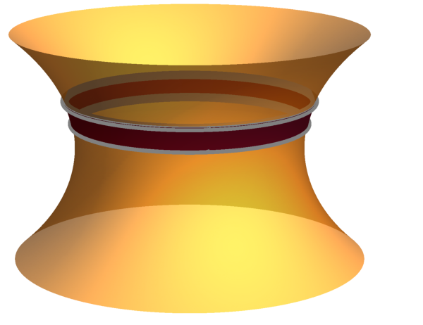
Refer to caption
Figure 3: An axisymmetric strip Σ\Sigma (shown in red, with its boundary curves in gray) on a catenoid.

We can use the divergence theorem to then replace the integral with two line integrals,

∫ΣⅆA​∇a(𝒇a⋅𝑿)=∫𝒞1ⅆϕ​ρ​𝒇a⋅𝑿​ta−∫𝒞2ⅆϕ​ρ​𝒇a⋅𝑿​ta=0,\int_{\Sigma}\rmd A\nabla_{a}(\boldsymbol{f}^{a}\cdot\boldsymbol{X})=\int_{\mathcal{C}_{1}}\rmd\phi~\rho\boldsymbol{f}^{a}\cdot\boldsymbol{X}t_{a}-\int_{\mathcal{C}_{2}}\rmd\phi~\rho\boldsymbol{f}^{a}\cdot\boldsymbol{X}t_{a}=0, (54)

where 𝒞1\mathcal{C}_{1} and 𝒞2\mathcal{C}_{2} are the upper and lower boundary curves of the strip, and tat_{a} is the surface vector tangent to the meridians. Since the patch of membrane was chosen arbitrarily, we conclude that the integral,

∫𝒞ⅆϕ​ρ​𝒇a⋅𝑿​ta=2​π​ρ​𝒇a⋅𝑿​ta\int_{\mathcal{C}}\rmd\phi~\rho\boldsymbol{f}^{a}\cdot\boldsymbol{X}t_{a}=2\pi\rho\boldsymbol{f}^{a}\cdot\boldsymbol{X}t_{a} (55)

is constant for all rings 𝒞\mathcal{C}.

Inserting our parametrization of the surface 𝑿=(ρ​cos⁡ϕ,ρ​sin⁡ϕ,z)T\boldsymbol{X}=(\rho\cos\phi,\rho\sin\phi,z)^{T}, we find

2​π​ρ​𝒇a⋅𝑿​ta\displaystyle 2\pi\rho\boldsymbol{f}^{a}\cdot\boldsymbol{X}t_{a} =π​kc​(ρ2​ψ′2​cos⁡ψ−tan⁡ψ⁡(sin⁡ψ−2​ρ​Ω0)−2​Ω0​z)\displaystyle=\pi k_{c}\left(\rho^{2}\psi^{\prime 2}\cos\psi-\tan\psi(\sin\psi-2\rho\Omega_{0})-2\Omega_{0}z\right) (56)
=π​kc​I+2​π​kc​Ω0​(ρ​tan⁡ψ−z),\displaystyle=\pi k_{c}I+2\pi k_{c}\Omega_{0}(\rho\tan\psi-z), (57)

where we have used the first integral in equation (8) to eliminate ψ′′\psi^{\prime\prime} terms in the stress tensor. Note that this constant does not require Ω0\Omega_{0} to vanish. One explanation for why it was necessary in the framework of the constructed Lagrangian to set Ω0=0\Omega_{0}=0 is the presence of the term proportional to z=∫ⅆ⁡ρ​tan⁡ψz=\int\rmd\rho\tan\psi. At the level of the Lagrangian for ψ⁡(ρ)\psi(\rho), there is no closed form for z⁡(ρ)z(\rho).

6 Conclusion

We have found the first integral of the second-order shape equation of axisymmetric lipid membranes with vanishing c0c_{0}, λ~\tilde{\lambda}, and p~\tilde{p}. In this case, (8) is invariant under conformal transformations. If we include any one of those parameters, such as c0c_{0}, it will break the scale invariance we used to find our first integral, likely making it impossible to solve the equation immediately. It is still an interesting challenge to find a first integral for non-vanishing c0c_{0}, λ~\tilde{\lambda}, and p~\tilde{p}.

We obtained the mechanical interpretation of the first integral by using the membrane stress tensor as in [13]. We find that the first integral II is proportional to 𝒇a⋅𝑿​ta\boldsymbol{f}^{a}\cdot\boldsymbol{X}t_{a} when Ω0=0\Omega_{0}=0, where tat_{a} is the surface vector tangent to the meridians of the surface.

Appendix A Detailed calculations for construction of first integrals

If η\eta, ξ\xi and BB do not explicitly depend on ψ′\psi^{\prime}, then (33) will be:

ρ​cos⁡ψ​F=0,\displaystyle\rho\cos\psi F=0, (58)

which means F=0F=0. And (34) is transformed into:

−ρ​cos⁡ψ​ξψ​ψ′3+[cos⁡ψ⁡(ξ−ρ​ξρ+2​ρ​ηψ)−ρ​sin⁡ψ​η]​ψ′2\displaystyle-\rho\cos{\psi}\xi_{\psi}\psi^{\prime 3}+\left[\cos{\psi}\left(\xi-\rho\xi_{\rho}+2\rho\eta_{\psi}\right)-\rho\sin{\psi}\eta\right]\psi^{\prime 2}
+[2​ρ​cos⁡ψ​ηρ−2​(Bψ+V​ξψ)]​ψ′−2​(V​ξρ+Vρ​ξ+Vψ​η+Bρ)=0\displaystyle+\left[2\rho\cos{\psi}\eta_{\rho}-2\left(B_{\psi}+V\xi_{\psi}\right)\right]\psi^{\prime}-2\left(V\xi_{\rho}+V_{\rho}\xi+V_{\psi}\eta+B_{\rho}\right)=0 (59)

We can separate the above equation into five independent equations according to the different orders of ψ′\psi^{\prime}:

ρ​cos⁡ψ​ξψ=0,\displaystyle\rho\cos{\psi}\xi_{\psi}=0, (60)
cos⁡ψ⁡(ξ−ρ​ξρ+2​ρ​ηψ)−ρ​sin⁡ψ​η=0,\displaystyle\cos{\psi}\left(\xi-\rho\xi_{\rho}+2\rho\eta_{\psi}\right)-\rho\sin{\psi}\eta=0, (61)
ρ​cos⁡ψ​ηρ−Bψ−V​ξψ=0,\displaystyle\rho\cos{\psi}\eta_{\rho}-B_{\psi}-V\xi_{\psi}=0, (62)
V​ξρ+Vρ​ξ+Vψ​η+Bρ=0.\displaystyle V\xi_{\rho}+V_{\rho}\xi+V_{\psi}\eta+B_{\rho}=0. (63)

From (60) and (61), we obtain:

η⁡(ρ,ψ)=C1​(ρ)cos⁡ψ​∫cos⁡ψ​ⅆψ+1cos⁡ψ​C2​(ρ),\displaystyle\eta(\rho,\psi)=\frac{C_{1}(\rho)}{\sqrt{\cos{\psi}}}\int\sqrt{\cos\psi}\rmd\psi+\frac{1}{\sqrt{\cos{\psi}}}C_{2}(\rho), (64)
ξ⁡(ρ)=C3​ρ+2​ρ​∫C1​(ρ)ρ​ⅆρ,\displaystyle\xi(\rho)=C_{3}\rho+2\rho\int{\frac{C_{1}(\rho)}{\rho}\rmd\rho}, (65)

Then from (62), (63), (31) and Bψ​ρ=Bρ​ψB_{\psi\rho}=B_{\rho\psi}, we have:

12{[35+56λ~ρ2−4(1+6λ~ρ2)cos2ψ+cos4ψ\displaystyle\frac{1}{2}\{[35+56\tilde{\lambda}\rho^{2}-4\left(1+6\tilde{\lambda}\rho^{2}\right)\cos{2\psi}+\cos{4\psi}
+8ρsinψ(−9c0−10Ω0+5p~ρ2+c0cos2ψ)]C1(ρ)\displaystyle+8\rho\sin{\psi}\left(-9c_{0}-10\Omega_{0}+5\tilde{p}\rho^{2}+c_{0}\cos{2\psi}\right)]C_{1}(\rho)
−32ρcos4ψ(C1′+ρC1′′)}∫cos⁡ψⅆψ\displaystyle-32\rho\cos^{4}{\psi}\left(C_{1}^{\prime}+\rho C_{1}^{\prime\prime}\right)\}\int\sqrt{\cos\psi}\rmd\psi
+[8ρ(C3+2∫C1​(ρ)ρⅆρ)\displaystyle+\left[8\rho\left(C_{3}+2\int{\frac{C_{1}(\rho)}{\rho}\rmd\rho}\right)\right.
(−c0−2​Ω0+3​p~​ρ2+c0​cos⁡2​ψ+4​λ~​ρ​sin⁡ψ)\displaystyle\left(-c_{0}-2\Omega_{0}+3\tilde{p}\rho^{2}+c_{0}\cos{2\psi}+4\tilde{\lambda}\rho\sin{\psi}\right)
+6​(−4​c0​ρ−8​Ω0​ρ+4​p~​ρ3+4​c0​ρ​cos⁡2​ψ+5​sin⁡ψCLOSE\displaystyle+6\left(-4c_{0}\rho-8\Omega_{0}\rho+4\tilde{p}\rho^{3}+4c_{0}\rho\cos{2\psi}+5\sin{\psi}\right.
+8λ~ρ2sinψ+sin3ψ)C1(ρ)](1−sin2ψ)sec⁡ψ\displaystyle\left.\left.+8\tilde{\lambda}\rho^{2}\sin{\psi}+\sin{3\psi}\right)C_{1}(\rho)\right]\left(1-\sin^{2}\psi\right)\sqrt{\sec\psi}
+C2​(ρ)2[35+56λ~ρ2−4(1+6λ~ρ2)cos2ψ+cos4ψ\displaystyle+\frac{C_{2}(\rho)}{2}\left[35+56\tilde{\lambda}\rho^{2}-4\left(1+6\tilde{\lambda}\rho^{2}\right)\cos{2\psi}+\cos{4\psi}\right.
+8ρ(−9c0−10Ω0+5p~ρ2+c0cos2ψ)sinψ]\displaystyle\left.+8\rho\left(-9c_{0}-10\Omega_{0}+5\tilde{p}\rho^{2}+c_{0}\cos{2\psi}\right)\sin{\psi}\right]
−16​ρ​cos4⁡ψ⁡(C2′+ρ​C2′′)=0.\displaystyle-16\rho\cos^{4}{\psi}\left(C_{2}^{\prime}+\rho C_{2}^{\prime\prime}\right)=0. (66)

As we have:

sec⁡ψ=(1−sin2⁡ψ)−14,\displaystyle\sqrt{\sec\psi}=(1-\sin^{2}\psi)^{-\frac{1}{4}}, (67)
∫cos⁡ψ​ⅆψ=∫(1−sin2⁡ψ)−14​ⅆ(sin⁡ψ),\displaystyle\int\sqrt{\cos\psi}\rmd\psi=\int(1-\sin^{2}\psi)^{-\frac{1}{4}}\rmd(\sin\psi), (68)

we can expand sec⁡ψ\sqrt{\sec\psi} and ∫cos⁡ψ​ⅆψ\int\sqrt{\cos\psi}\rmd\psi in terms of sin⁡ψ\sin\psi:

sec⁡ψ=∑n=0∞Γ⁡(n+14)Γ⁡(14)​Γ​(n+1)​sin2​n⁡ψ,\displaystyle\sqrt{\sec\psi}=\sum_{n=0}^{\infty}\frac{\Gamma(n+\frac{1}{4})}{\Gamma(\frac{1}{4})\Gamma(n+1)}\sin^{2n}\psi, (69)
∫cos⁡ψ​ⅆψ=G+∑n=0∞Γ⁡(n+14)(2​n+1)​Γ​(14)​Γ​(n+1)​sin2​n+1⁡ψ,\displaystyle\int\sqrt{\cos\psi}\rmd\psi=G+\sum_{n=0}^{\infty}\frac{\Gamma(n+\frac{1}{4})}{(2n+1)\Gamma(\frac{1}{4})\Gamma(n+1)}\sin^{2n+1}\psi, (70)

where GG in (70) is an integral constant. Then we can write (66) in terms of sin⁡ψ\sin\psi:

∑n=04θn​sinn⁡ψ+∑n=0∞Θn​sin2​n+5⁡ψ+∑n=0∞Λn​sin2​n+6⁡ψ=0,\displaystyle\sum_{n=0}^{4}\theta_{n}\sin^{n}\psi+\sum_{n=0}^{\infty}\Theta_{n}\sin^{2n+5}\psi+\sum_{n=0}^{\infty}\Lambda_{n}\sin^{2n+6}\psi=0, (71)

where

θ0=8​ρ​[(−2​Ω0+3​p~​ρ2)​(C3+2​∫C1​(ρ)ρ​ⅆρ)+3​(−2​Ω+p~​ρ2)​C1​(ρ)]\displaystyle\theta_{0}=8\rho\left[\left(-2\Omega_{0}+3\tilde{p}\rho^{2}\right)\left(C_{3}+2\int\frac{C_{1}(\rho)}{\rho}\rmd\rho\right)+3\left(-2\Omega+\tilde{p}\rho^{2}\right)C_{1}(\rho)\right]
+16​G​[(1+λ~​ρ2)​C1​(ρ)−ρ⁡(C1′+ρ​C1′′)]\displaystyle+16G\left[\left(1+\tilde{\lambda}\rho^{2}\right)C_{1}(\rho)-\rho\left(C_{1}^{\prime}+\rho C_{1}^{\prime\prime}\right)\right]
+16​[(1+λ~​ρ2)​C2​(ρ)−ρ⁡(C2′+ρ​C2′′)],\displaystyle+16\left[\left(1+\tilde{\lambda}\rho^{2}\right)C_{2}(\rho)-\rho\left(C_{2}^{\prime}+\rho C_{2}^{\prime\prime}\right)\right], (72)
θ1=64​λ~​ρ2​∫C1​(ρ)ρ​ⅆρ+[64​(1+λ~​ρ2)+4​G​ρ​(−8​c0−10​η0+5​p~​ρ2)]​C1​(ρ)\displaystyle\theta_{1}=64\tilde{\lambda}\rho^{2}\int\frac{C_{1}(\rho)}{\rho}\rmd\rho+\left[64\left(1+\tilde{\lambda}\rho^{2}\right)+4G\rho\left(-8c_{0}-10\eta_{0}+5\tilde{p}\rho^{2}\right)\right]C_{1}(\rho)
+4​ρ​[8​C3​λ~​ρ+(−8​c0−10​Ω0+5​p~​ρ2)​C2​(ρ)−4​C1′−4​ρ​C1′′],\displaystyle+4\rho\left[8C_{3}\tilde{\lambda}\rho+\left(-8c_{0}-10\Omega_{0}+5\tilde{p}\rho^{2}\right)C_{2}(\rho)-4C_{1}^{\prime}-4\rho C_{1}^{\prime\prime}\right], (73)
θ2=−2ρ[8C3c0−6C3Ω0+9C3p~ρ2+2(8c0−6Ω0+9p~ρ2)∫C1​(ρ)ρⅆρ\displaystyle\theta_{2}=-2\rho\left[8C_{3}c_{0}-6C_{3}\Omega_{0}+9C_{3}\tilde{p}\rho^{2}+2\left(8c_{0}-6\Omega_{0}+9\tilde{p}\rho^{2}\right)\int\frac{C_{1}(\rho)}{\rho}\rmd\rho\right.
+(40​c0+2​Ω0−12​G​λ~​ρ−p~​ρ2)​C1​(ρ)−16​G​(C1′+ρ​C1′′)\displaystyle+\left(40c_{0}+2\Omega_{0}-12G\tilde{\lambda}\rho-\tilde{p}\rho^{2}\right)C_{1}(\rho)-16G\left(C_{1}^{\prime}+\rho C_{1}^{\prime\prime}\right)
−16C2′−4ρ(3λ~C2(ρ)+4C2′′)],\displaystyle\left.-16C_{2}^{\prime}-4\rho\left(3\tilde{\lambda}C_{2}(\rho)+4C_{2}^{\prime\prime}\right)\right], (74)
θ3=−43[18C3λ~ρ2+44C1(ρ)+ρ(36λ~ρ∫C1​(ρ)ρⅆρ+6c0C2(ρ)\displaystyle\theta_{3}=-\frac{4}{3}\left[18C_{3}\tilde{\lambda}\rho^{2}+44C_{1}(\rho)+\rho\left(36\tilde{\lambda}\rho\int\frac{C_{1}(\rho)}{\rho}\rmd\rho+6c_{0}C_{2}(\rho)\right.\right.
+8λ~ρC1(ρ)+6c0GC1(ρ)−23C1′−23ρC1′′)],\displaystyle\left.\left.+8\tilde{\lambda}\rho C_{1}(\rho)+6c_{0}GC_{1}(\rho)-23C_{1}^{\prime}-23\rho C_{1}^{\prime\prime}\right)\right], (75)
θ4=912​C3​ρ​(16​c0+2​Ω0−3​p~​ρ2)+4​C2​(ρ)+32​ρ​(16​c0+2​Ω0−3​p~​ρ2)\displaystyle\theta_{4}=\frac{9}{12}C_{3}\rho\left(16c_{0}+2\Omega_{0}-3\tilde{p}\rho^{2}\right)+4C_{2}(\rho)+\frac{3}{2}\rho\left(16c_{0}+2\Omega_{0}-3\tilde{p}\rho^{2}\right)
∫C1​(ρ)ρ​ⅆρ+ρ12​(304​c0+14​Ω0−7​p~​ρ2)​C1​(ρ)+4​G​C1​(ρ)\displaystyle\int\frac{C_{1}(\rho)}{\rho}\rmd\rho+\frac{\rho}{12}\left(304c_{0}+14\Omega_{0}-7\tilde{p}\rho^{2}\right)C_{1}(\rho)+4GC_{1}(\rho)
−16​G​ρ​(C1′+ρ​C1′′)−16​ρ​(C2′+ρ​C2′′),\displaystyle-16G\rho\left(C_{1}^{\prime}+\rho C_{1}^{\prime\prime}\right)-16\rho\left(C_{2}^{\prime}+\rho C_{2}^{\prime\prime}\right), (76)
Θn=1Γ⁡(14)​Γ​(n+3){−48λ~Γ(n+54)ρ2∫C1​(ρ)ρⅆρ+[−6C3λ~(2n+1)(2n+3)\displaystyle\Theta_{n}=\frac{1}{\Gamma(\frac{1}{4})\Gamma(n+3)}\left\{-48\tilde{\lambda}\Gamma\left(n+\frac{5}{4}\right)\rho^{2}\int\frac{C_{1}(\rho)}{\rho}\rmd\rho+\left[-6C_{3}\tilde{\lambda}(2n+1)(2n+3)\right.\right.
(2​n+5)​(4​n+1)​ρ2−4​(−135−348​n−172​n2+24​n3+16​n4)​C1​(ρ)\displaystyle(2n+5)(4n+1)\rho^{2}-4\left(-135-348n-172n^{2}+24n^{3}+16n^{4}\right)C_{1}(\rho)
−4​(n+3)​(2​n+1)​(4​n+1)​(4​n+5)​λ~​ρ2​C1​(ρ)−ρ⁡(415+792​n+308​n2)\displaystyle-4(n+3)(2n+1)(4n+1)(4n+5)\tilde{\lambda}\rho^{2}C_{1}(\rho)-\rho(415+792n+308n^{2})
(C1′+ρC1′′)]Γ⁡(n+14)(2​n+1)​(2​n+3)​(2​n+5)},\displaystyle\left.\left.(C_{1}^{\prime}+\rho C_{1}^{\prime\prime})\right]\frac{\Gamma\left(n+\frac{1}{4}\right)}{(2n+1)(2n+3)(2n+5)}\right\}, (77)
Λn=Γ⁡(n+54)​ρ2​Γ​(14)​Γ​(n+4){6[8c0(n+3)+(4n+5)(2Ω−3p~ρ2)]∫C1​(ρ)ρⅆρ\displaystyle\Lambda_{n}=\frac{\Gamma\left(n+\frac{5}{4}\right)\rho}{2\Gamma\left(\frac{1}{4}\right)\Gamma(n+4)}\left\{6\left[8c_{0}(n+3)+(4n+5)\left(2\Omega-3\tilde{p}\rho^{2}\right)\right]\int\frac{C_{1}(\rho)}{\rho}\rmd\rho\right.
+[3C3(2n+3)(2n+5)(8c0(n+3)+(4n+5)(2Ω0−3p~ρ2))\displaystyle+\left[3C_{3}(2n+3)(2n+5)\left(8c_{0}(n+3)+(4n+5)\left(2\Omega_{0}-3\tilde{p}\rho^{2}\right)\right)\right.
+(8​c0​(n+3)​(85+82​n+16​n2)+(2​n+3)​(4​n+5)​(8​n+15)CLOSE\displaystyle+\left(8c_{0}\left(n+3\right)\left(85+82n+16n^{2}\right)+(2n+3)(4n+5)(8n+15)\right.
(2Ω−p~ρ2))C1(ρ)]1(2​n+3)​(2​n+5)}.\displaystyle\left.\left.\left.(2\Omega-\tilde{p}\rho^{2})\right)C_{1}(\rho)\right]\frac{1}{(2n+3)(2n+5)}\right\}. (78)

And (71) is equivalent to seven independent equations according to the order of sin⁡ψ\sin\psi:

θ0=θ1=θ2=θ3=θ4=Θn=Λn=0,\displaystyle\theta_{0}=\theta_{1}=\theta_{2}=\theta_{3}=\theta_{4}=\Theta_{n}=\Lambda_{n}=0, (79)

which leads to the following equations:

ρ⁡[(−2​Ω0+3​p~​ρ2)​(C3+2​∫C1​(ρ)ρ​ⅆρ)+3​(−2​Ω0+p~​ρ2)​C1​(ρ)]\displaystyle\rho\left[\left(-2\Omega_{0}+3\tilde{p}\rho^{2}\right)\left(C_{3}+2\int\frac{C_{1}(\rho)}{\rho}\rmd\rho\right)+3\left(-2\Omega_{0}+\tilde{p}\rho^{2}\right)C_{1}(\rho)\right]
+2​G​[(1+λ~​ρ2)​C1​(ρ)−ρ⁡(C1′+ρ​C1′′)]\displaystyle+2G\left[\left(1+\tilde{\lambda}\rho^{2}\right)C_{1}(\rho)-\rho\left(C_{1}^{\prime}+\rho C_{1}^{\prime\prime}\right)\right]
+2​[(1+λ~​ρ2)​C2​(ρ)−ρ⁡(C2′+ρ​C2′′)]=0,\displaystyle+2\left[\left(1+\tilde{\lambda}\rho^{2}\right)C_{2}(\rho)-\rho\left(C_{2}^{\prime}+\rho C_{2}^{\prime\prime}\right)\right]=0, (80)
16​λ~​ρ2​∫C1​(ρ)ρ​ⅆρ+[16​(1+λ~​ρ2)+G​ρ​(−8​c0−10​η0+5​p~​ρ2)]​C1​(ρ)\displaystyle 16\tilde{\lambda}\rho^{2}\int\frac{C_{1}(\rho)}{\rho}\rmd\rho+\left[16\left(1+\tilde{\lambda}\rho^{2}\right)+G\rho\left(-8c_{0}-10\eta_{0}+5\tilde{p}\rho^{2}\right)\right]C_{1}(\rho)
+8​C3​λ~​ρ2+ρ⁡(−8​c0−10​Ω0+5​p~​ρ2)​C2​(ρ)−4​ρ​C1′−4​ρ2​C1′′=0,\displaystyle+8C_{3}\tilde{\lambda}\rho^{2}+\rho\left(-8c_{0}-10\Omega_{0}+5\tilde{p}\rho^{2}\right)C_{2}(\rho)-4\rho C_{1}^{\prime}-4\rho^{2}C_{1}^{\prime\prime}=0, (81)
8​C3​c0−6​C3​Ω0+9​C3​p~​ρ2+2​(8​c0−6​Ω0+9​p~​ρ2)​∫C1​(ρ)ρ​ⅆρ\displaystyle 8C_{3}c_{0}-6C_{3}\Omega_{0}+9C_{3}\tilde{p}\rho^{2}+2\left(8c_{0}-6\Omega_{0}+9\tilde{p}\rho^{2}\right)\int\frac{C_{1}(\rho)}{\rho}\rmd\rho
+(40​c0+2​Ω0−12​G​λ~​ρ−p~​ρ2)​C1​(ρ)−16​G​(C1′+ρ​C1′′)\displaystyle+\left(40c_{0}+2\Omega_{0}-12G\tilde{\lambda}\rho-\tilde{p}\rho^{2}\right)C_{1}(\rho)-16G\left(C_{1}^{\prime}+\rho C_{1}^{\prime\prime}\right)
−16​C2′−4​ρ​(3​λ~​C2​(ρ)+4​C2′′)=0,\displaystyle-16C_{2}^{\prime}-4\rho\left(3\tilde{\lambda}C_{2}(\rho)+4C_{2}^{\prime\prime}\right)=0, (82)
18​C3​λ~​ρ2+44​C1​(ρ)+ρ⁡(36​λ~​ρ​∫C1​(ρ)ρ​ⅆρ+6​c0​C2​(ρ)CLOSE\displaystyle 18C_{3}\tilde{\lambda}\rho^{2}+44C_{1}(\rho)+\rho\left(36\tilde{\lambda}\rho\int\frac{C_{1}(\rho)}{\rho}\rmd\rho+6c_{0}C_{2}(\rho)\right.
OPEN+8​λ~​ρ​C1​(ρ)+6​c0​G​C1​(ρ)−23​C1′−23​ρ​C1′′)=0,\displaystyle\left.+8\tilde{\lambda}\rho C_{1}(\rho)+6c_{0}GC_{1}(\rho)-23C_{1}^{\prime}-23\rho C_{1}^{\prime\prime}\right)=0, (83)
9​C3​ρ​(16​c0+2​Ω0−3​p~​ρ2)+48​C2​(ρ)+18​ρ​(16​c0+2​Ω0−3​p~​ρ2)\displaystyle 9C_{3}\rho\left(16c_{0}+2\Omega_{0}-3\tilde{p}\rho^{2}\right)+48C_{2}(\rho)+18\rho\left(16c_{0}+2\Omega_{0}-3\tilde{p}\rho^{2}\right)
∫C1​(ρ)ρ​ⅆρ+ρ⁡(304​c0+14​Ω0−7​p~​ρ2)​C1​(ρ)\displaystyle\int\frac{C_{1}(\rho)}{\rho}\rmd\rho+\rho\left(304c_{0}+14\Omega_{0}-7\tilde{p}\rho^{2}\right)C_{1}(\rho)
+48​G​C1​(ρ)−192​G​ρ​(C1′+ρ​C1′′)−192​ρ​(C2′+ρ​C2′′)=0,\displaystyle+48GC_{1}(\rho)-192G\rho\left(C_{1}^{\prime}+\rho C_{1}^{\prime\prime}\right)-192\rho\left(C_{2}^{\prime}+\rho C_{2}^{\prime\prime}\right)=0, (84)
−12λ~(4n+1)(2n+1)(2n+3)(2n+5)ρ2∫C1​(ρ)ρⅆρ\displaystyle-12\tilde{\lambda}(4n+1)(2n+1)(2n+3)(2n+5)\rho^{2}\int\frac{C_{1}(\rho)}{\rho}\rmd\rho
−6​C3​λ~​(2​n+1)​(2​n+3)​(2​n+5)​(4​n+1)​ρ2\displaystyle-6C_{3}\tilde{\lambda}(2n+1)(2n+3)(2n+5)(4n+1)\rho^{2}
−4[−135−348n−172n2+24n3+16n4\displaystyle-4\left[-135-348n-172n^{2}+24n^{3}+16n^{4}\right.
+(n+3)(2n+1)(4n+1)(4n+5)λ~ρ2]C1(ρ)\displaystyle\left.+(n+3)(2n+1)(4n+1)(4n+5)\tilde{\lambda}\rho^{2}\right]C_{1}(\rho)
−ρ⁡(415+792​n+308​n2)​(C1′+ρ​C1′′)=0,\displaystyle-\rho(415+792n+308n^{2})(C_{1}^{\prime}+\rho C_{1}^{\prime\prime})=0, (85)
6​(2​n+3)​(2​n+5)​[8​c0​(n+3)+(4​n+5)​(2​Ω0−3​p~​ρ2)]​∫C1​(ρ)ρ​ⅆρ\displaystyle 6(2n+3)(2n+5)\left[8c_{0}(n+3)+(4n+5)\left(2\Omega_{0}-3\tilde{p}\rho^{2}\right)\right]\int\frac{C_{1}(\rho)}{\rho}\rmd\rho
+3​C3​(2​n+3)​(2​n+5)​[8​c0​(n+3)+(4​n+5)​(2​Ω0−3​p~​ρ2)]\displaystyle+3C_{3}(2n+3)(2n+5)\left[8c_{0}(n+3)+(4n+5)\left(2\Omega_{0}-3\tilde{p}\rho^{2}\right)\right]
+[8c0(n+3)(85+82n+16n2)+(2n+3)(4n+5)(8n+15)\displaystyle+\left[8c_{0}\left(n+3\right)\left(85+82n+16n^{2}\right)+(2n+3)(4n+5)(8n+15)\right.
(2Ω0−p~ρ2)]C1(ρ)=0.\displaystyle\left.(2\Omega_{0}-\tilde{p}\rho^{2})\right]C_{1}(\rho)=0. (86)

We note that (85) and (86) should valid for any non-negative integer nn, and expressions of C1​(ρ)C_{1}(\rho) and C2​(ρ)C_{2}(\rho) do not contain nn. Then we investigate the coefficient of n3n^{3} and n4n^{4} in (85), which should be zero separately, and lead to two equations:

−912​λ~​ρ2​(C3+2​∫C1​(ρ)ρ​ⅆρ)−32​(3+20​λ~​ρ2)​C1​(ρ)=0,\displaystyle-912\tilde{\lambda}\rho^{2}\left(C_{3}+2\int\frac{C_{1}(\rho)}{\rho}\rmd\rho\right)-32\left(3+20\tilde{\lambda}\rho^{2}\right)C_{1}(\rho)=0, (87)
−192​λ~​ρ2​(C3+2​∫C1​(ρ)ρ​ⅆρ)−64​(1+2​λ~​ρ2)​C1​(ρ)=0.\displaystyle-192\tilde{\lambda}\rho^{2}\left(C_{3}+2\int\frac{C_{1}(\rho)}{\rho}\rmd\rho\right)-64\left(1+2\tilde{\lambda}\rho^{2}\right)C_{1}(\rho)=0. (88)

Canceling C3+2​∫C1​(ρ)ρ​ⅆρC_{3}+2\int\frac{C_{1}(\rho)}{\rho}\rmd\rho both in (87) and (88), we have:

(2​λ~​ρ2−13)​C1​(ρ)=0,\displaystyle(2\tilde{\lambda}\rho^{2}-13)C_{1}(\rho)=0, (89)

which leaves us no choice but C1​(ρ)=0C_{1}(\rho)=0, and hence C3​λ~=0C_{3}\tilde{\lambda}=0. Then (80)–(84) will become as:

2​(1+λ~​ρ2)​C2​(ρ)+ρ⁡(3​C3​p~​ρ2−2​C3​Ω0−2​C2′−2​ρ​C2′′)=0,\displaystyle 2\left(1+\tilde{\lambda}\rho^{2}\right)C_{2}(\rho)+\rho\left(3C_{3}\tilde{p}\rho^{2}-2C_{3}\Omega_{0}-2C_{2}^{\prime}-2\rho C_{2}^{\prime\prime}\right)=0, (90)
(5​p~​ρ2−8​c0−10​Ω0)​C2​(ρ)=0,\displaystyle\left(5\tilde{p}\rho^{2}-8c_{0}-10\Omega_{0}\right)C_{2}(\rho)=0, (91)
8​C3​c0−6​C3​Ω0+9​C3​p~​ρ2−12​λ~​ρ​C2​(ρ)−16​(C2′+ρ​C2′′)=0,\displaystyle 8C_{3}c_{0}-6C_{3}\Omega_{0}+9C_{3}\tilde{p}\rho^{2}-12\tilde{\lambda}\rho C_{2}(\rho)-16\left(C_{2}^{\prime}+\rho C_{2}^{\prime\prime}\right)=0, (92)
c0​C2​(ρ)=0,\displaystyle c_{0}C_{2}(\rho)=0, (93)
3​C3​ρ​(16​c0+2​Ω0−3​p~​ρ2)+16​C2​(ρ)−64​ρ​(C2′+ρ​C2′′)=0.\displaystyle 3C_{3}\rho\left(16c_{0}+2\Omega_{0}-3\tilde{p}\rho^{2}\right)+16C_{2}(\rho)-64\rho\left(C_{2}^{\prime}+\rho C_{2}^{\prime\prime}\right)=0. (94)

Canceling ρ⁡(C2′+ρ​C2′′)\rho(C_{2}^{\prime}+\rho C_{2}^{\prime\prime}) both in (90) and (92), we can solve C2​(ρ)C_{2}(\rho) as:

C2​(ρ)=C3​ρ​(8​c0+10​Ω0−15​p~​ρ2)4​(4+7​λ~​ρ2).\displaystyle C_{2}(\rho)=\frac{C_{3}\rho\left(8c_{0}+10\Omega_{0}-15\tilde{p}\rho^{2}\right)}{4\left(4+7\tilde{\lambda}\rho^{2}\right)}. (95)

Canceling ρ⁡(C2′+ρ​C2′′)\rho(C_{2}^{\prime}+\rho C_{2}^{\prime\prime}) both in (90) and (94), we can solve C2​(ρ)C_{2}(\rho) as:

C2​(ρ)=C3​ρ​(48​c0+70​Ω0−105​p~​ρ2)16​(3+4​λ~​ρ2).\displaystyle C_{2}(\rho)=\frac{C_{3}\rho\left(48c_{0}+70\Omega_{0}-105\tilde{p}\rho^{2}\right)}{16\left(3+4\tilde{\lambda}\rho^{2}\right)}. (96)

If C3=0C_{3}=0, then C2​(ρ)=0C_{2}(\rho)=0, which leads to a trivial solution of the first integral. So we should assume C3≠0C_{3}\neq 0, and hence λ~=0\tilde{\lambda}=0, in our discussion. With combining (95) and (96), we have:

6​c0+10​Ω0−15​p~​ρ2=0,\displaystyle 6c_{0}+10\Omega_{0}-15\tilde{p}\rho^{2}=0, (97)

which leads to :

p~=0,Ω0=−35​c0.\displaystyle\tilde{p}=0,\quad\Omega_{0}=-\frac{3}{5}c_{0}. (98)

Then we have:

C2​(ρ)=c0​C38​ρ.\displaystyle C_{2}(\rho)=\frac{c_{0}C_{3}}{8}\rho. (99)

And because of (93) we have:

c0​C2​(ρ)=c02​C38​ρ=0,\displaystyle c_{0}C_{2}(\rho)=\frac{c_{0}^{2}C_{3}}{8}\rho=0, (100)

which leaves:

c0=Ω0=p~=C2​(ρ)=0.\displaystyle c_{0}=\Omega_{0}=\tilde{p}=C_{2}(\rho)=0. (101)

And it is exactly the solution of (66), we could check this by substituting C1​(ρ)=C2​(ρ)=c0=λ~=p~=Ω0=0C_{1}(\rho)=C_{2}(\rho)=c_{0}=\tilde{\lambda}=\tilde{p}=\Omega_{0}=0 into (66).

So the non-trivial solution for (66) only exists in the case of vanishing c0c_{0}, λ~\tilde{\lambda}, p~\tilde{p} and Ω0\Omega_{0}:

C1​(ρ)=C2​(ρ)=0,C3≠0,\displaystyle C_{1}(\rho)=C_{2}(\rho)=0,\quad C_{3}\neq 0, (102)

which leaves the only solution for (59):

B=0,η=0,ξ=C3​ρ.\displaystyle B=0,\quad\eta=0,\quad\xi=C_{3}\rho. (103)
The authors are grateful for the valuable and inspiring discussions with Ping Ao. We thank Markus Deserno for his insightful suggestions. The authors are also grateful for financial support from the National Natural Science Foundation of China (Grant No. 11274046) and the National Science Foundation of the United States (award No. 1515007).

References

  • [1] Poisson S 1833 Traité de Mécanique (Bachelier, Paris)
  • [2] Fernando C M and André N 2014 Ann. Math. 179 683
  • [3] Tek S 2007 Journal of Mathematical Physics 48 013505
  • [4] Helfrich W 1973 Z. Naturforsch. C 28 693
  • [5] Ou-Yang Z C and Helfrich W 1987 Phys. Rev. Lett. 59 2486
  • [6] Ou-Yang Z C and Helfrich W 1989 Phys. Rev. A 39 5280
  • [7] Konopelchenko B G 1997 Physics Letters B 414 58
  • [8] Lipowsky R 1991 Nature 349 475
  • [9] Landolfi G 2003 Journal of Physics A: Mathematical and General 36 11937
  • [10] Deuling H J and Helfrich W 1976 Biophysical Journal 16 861
  • [11] Seifert U 1997 Advances in Physics 46 13
  • [12] Ou-Yang Z C, Liu J X and Xie Y Z 1999 Geometric Methods in the Elastic Theory of Membranes in Liquid Crystal Phases (Singapore: World Scientific)
  • [13] Capovilla R and Guven J 2002 Journal of Physics A: Mathematical and General 35 6233
  • [14] Capovilla R, Guven J and Santiago J A 2003 Journal of Physics A: Mathematical and General 36 6281
  • [15] Capovilla R and Guven J 2004 Journal of Physics: Condensed Matter 16 S2187
  • [16] Capovilla R, Guven J and Rojas E 2005 Journal of Physics A: Mathematical and General 38 8201
  • [17] Capovilla R, Guven J and Rojas E 2005 Journal of Physics A: Mathematical and General 38 8841
  • [18] Tu Z C and Ou-Yang Z C 2004 Journal of Physics A: Mathematical and General 37 11407
  • [19] Tu Z C 2013 Chinese Physics B 22 28701
  • [20] Hu J G and Ou-Yang Z C 1993 Phys. Rev. E 47 461
  • [21] Zheng W M and Liu J X 1993 Phys. Rev. E 48 2856
  • [22] Naito H, Okuda M and Ou-Yang Z C 1995 Phys. Rev. Lett. 74 4345
  • [23] Mladenov I M 2002 Eur. Phys. J. B 29 327
  • [24] Ou-Yang Z C 1990 Phys. Rev. A 41 4517
  • [25] Ou-Yang Z C 1993 Phys. Rev. E 47 747
  • [26] Castro-Villarreal P and Guven J 2007 Phys. Rev. E 76 011922
  • [27] Zhang S G and Ou-Yang Z C 1996 Phys. Rev. E 53 4206
  • [28] Vassilev V M, Djondjorov P A and Mladenov I M 2008 Journal of Physics A: Mathematical and General 41 435201
  • [29] Zhou X H 2010 Chinese Physics B 19 58702
  • [30] Naito H, Okuda M and Ou-Yang Z C 1993 Phys. Rev. E 48 2304
  • [31] Naito H, Okuda M and Ou-Yang Z C 1996 Phys. Rev. E 54 2816
  • [32] Ibragimov N H 1969 Theor. Math. Phys. 1 267
  • [33] Vassilev V M and Mladenov I M 2004 Geometric Symmetry Groups, Conservation Laws and Group-Invariant Solutions of the Willmore Equation Proceedings of the Fifth International Conference on Geometry, Integrability and Quantization (Sofia, Bulgaria: Softex) p 246
  • [34] Vassilev V M, Djondjorov P A, Atanassov E, Hadzhilazova M T and Mladenov I M 2014 AIP Conference Proceedings 1629 201
  • [35] Müller M M, Deserno M and Guven J 2005 Phys. Rev. E 72 061407