Time-scale characteristics of Kasaï river hydrological regime variability for 1940-1999
Abstract
The present study was undertaken with the aim of contributing to the characterization of the nonstationary variability of the hydrological regime of the Kasaï River using the wavelet analysis for 1940-1999. The rainfalls and discharge over Kasaï Basin have marked fluctuations with a perceptible downward trend and some shift around 1950, 1960, 1970, 1983 and 1994. The results show that rainfalls over Kasaï basin and the discharge at Ilebo station patterns exhibit a strong annual oscillation and some intermittent oscillations in 2-8 years (1950-1975, 1983-1995) and 8-16 years (1970-1999) time scales. The wavelet coherence analysis reveals a weak possible connection between hydrological variables (rainfalls, discharge) and climate indices relative to sea surface temperature and atmospheric circulation over Atlantic tropical, Indian and Pacific Oceans (coherence less than 0.55).
KEYWORDS: wavelet transform, coherence analysis, rainfall, discharge, climate indices.
Department of Physics, University of Kinshasa, B.P. 190 Kinshasa XI, DR Congo
1 INTRODUCTION
The Kasaï river is the chief southern tributary of the Congo River, into which, at Kwamouth, Congo (Kinshasa), 200 km above Malebo (Stanley) Pool, it empties a volume approaching one-fifth that of the main stream. This stretch is interrupted by several spectacular rapids and waterfalls, the river flowing in deeply trenched valleys at elevations of about 600–900 m. The Kasaï River eventually crosses a further series of rapids and falls, broadening and deepening to make navigation possible.
For effective and sustainable management of water resources in the Kasaï basin the knowledge of their availability and their variability is needed. It is also an important indication for modeling and exploration of the evolution of water resources of this region. In order to improve the understanding of the influence of various factors on the evolution of the hydrological response of the Kasaï, and more broadly on the development of water resources, from the regional to a global scale, Kasaï watershed has been subject of few studies undertaken by De Baker [1], Devroey [2] who provided a lot of information’s about Kasaï basin. Ntombi et al. [3] and Kisangala et al. [4] have focused on statistical analyzes based on existing data to establish an understanding of hydrology of the basin.
In the context of climate change, the determination of preferential scales between climate variability and hydrological variability of Kasaï watershed is needed. The overall variability of short-term climate is generally associated with phases of oceanic and atmospheric phenomena coupled with El Niño (ENSO) and the North Atlantic Oscillation (NAO). While El Niño Southern Oscillation (ENSO) affects weather and climate variability around the world, the North Atlantic Oscillation (NAO) is the climate dominant mode in the region of the North Atlantic. These oscillations have been used in several studies to develop accurate models able to predict climate variability.The determination of the climate change impact on hydrological systems and their water resources constitutes a major issue of the 21st century for which scientists must answer.
The main objectives are to:
- —
identify and quantify the main modes of variability of the climate and hydrological response of Kasaï river basin;
- —
characterize the relationships between discharge at Ilebo’s station, gridded rainfall over Kasaï basin signals and some climate indices.
2 STUDY AREA AND DATA
Kasaï basin covers an area of 904,000 square kilometers, between longitudes 15.75 ° and 24.7 ° east and between 0.75 ° South and 12.25 ° South latitude (Fig. 1). 72.4% of this basin is in DR Congo and the remaining 27.6%, representing the Southwest part is located in Angola.

From orographic point of view (Fig. 1), one can identified a depression, sprinkled with few isolated massifs, at the North of the basin around the 4th parallel which is between 300 and 500 meters of altitude. The trays exceeding the altitude of 1000 meters are located on the western edge of the basin between Wamba and Loange, to the south, as well as in the Southeast part. The rapids that cut most of the major tributaries of the basin are located between the plateau at 500 meters of altitude and the central depression.
The longest river in the southern Congo River basin system, the Kasaï River, measures 2,153 km from its source on the eastern slope of the Bie Plateau in Angola by 12 ° South and 19 ° East longitude Greenwich, near the plateau 1500 meters above sea level where the Zambezi River also takes its origins [2] to Kwamouth. The Kasaï River is the largest tributary of the Congo River. It swells waters of many tributaries whose some of them measure themselves more than 1,000 kilometers.
Its headstream runs east for 250 miles (402 km), then turns north for nearly 300 miles (483 km) to form the frontier between Angola and Congo. Traffic is especially heavy on the 510-mile- (820-kilometre-) long waterway from Kinshasa to Ilebo. Above Ilebo, navigation is impeded by sandbanks, but shallow-draft boats can reach Djokupunda. There the Mai- Munene Falls require goods to be carried 40 miles (64 km) by rail to the next navigable reach, from Mukumbi to Mai- Munene. In its lower reaches, the river enters the equatorial rainforest. Below its confluence with the Kwango, it forms Wissmann Pool and then receives the Fimi-Lukenie, bringing the waters of Lake Mai-Ndombe. Thereafter, it is known as the Kwa.
The climate is equatorial in the northern part of Kasaï basin. It is characterized by little difference in seasons, with high temperature and humidity virtually constant. The rainfall distribution throughout the year is on average around 1500 millimeters.


In the South, there is the tropical climate of the Sudan type with two maxima of rainfall and temperature; the dry season becomes longer as one progresses from the north towards the south in the basin. The relief of the southern region of Kasaï basin causes a slight temperature drop.
Variations in the length of the rainy season depending on the latitude are clearly demonstrated by the graph in Fig. 6. This basin had 38 weather stations in the colonial era. The mean maximum and minimum absolute temperatures are respectively 32 °/27 °C and 21 °/13 °C in the north/south of Kasaï basin (Fig. 4).

The great equatorial forest covers just about any depression of the central basin until about the 5th parallel; it pushes its ramifications as wide wooded galleries, going up through the valleys of Kwilu, Kasaï and Lulua until the 7th parallel.
Climate data
Gridded rainfall (1940-1999) were extracted from the African gridded data set from the SIEREM database [5] provided by the HydroSciences Montpellier Laboratory on the basis of several data sources, including the former ORSTOM (now IRD – Institut de Recherche pour le Développement) rainfall database [6]. This data set SIEREM.v1 was constructed from SIEREM database by kriging interpolation. SIEREM is an environmental information system for water resources. Raw historical climate datasets are not appropriate for statistical analysis because of inhomogeneity and leakage while gridded datasets have undergone rigorous quality control and have been homogenized [7, 8].
Climate indices used are listed in table 1.
| Climate indices | Data | Periods | Source |
|---|---|---|---|
| NAO | North Atlantic Oscillation [9] | 1950-2013 | “Earth System Research Laboratory (ESRL) |
| Nino 3.4 | East Central Tropical Pacific SST Index [10] | 1951-2013 | of the National Oceanic and |
| TNA | Tropical Northern Atlantic Index [11] | 1948-2013 | Atmospheric Administration (NOAA)” |
| TSA | Tropical Southern Atlantic Index [11] | 1948-2013 | web page http://www.cpc.ncep.noaa.gov/data/ind ices/ |
| Solar | Solar Flux [12] | 1948-2014 | |
| DMI | Dipole Mode Index [13] | 1870-2014 | The Frontier Research Center for Global Change |
| (JAMSTEC, Japan)” web page | |||
| (http://www.jamstec.go.jp/frcgc/resear ch/d | |||
| 1/iod/HTML/Dipole%20Mode%20In dex.html) |
3 METHODS
Characterization of the hydrological variability (discharge), the rainfall fluctuations and their comparison with the climate indices are performed by using the signal processing methods (multitaper, wavelet analysis,…).
Climate variability refers to the climatic parameter of a region varying from its long-term mean. Every year in a specific time period, the climate of a location is different. Some years have below average rainfall, others have average or above average rainfall.

3.1 HIERARCHICAL CLUSTERING ON PRINCIPAL COMPONENTS
3.2 THE SEGMENTATION METHOD OF HILBERT
The time series segmentation procedure in this case gives several changes of average. By using a specific algorithm, one or more shift dates (if any) which separate adjacent segments whose averages have a significant difference under the Scheffe test are selected [16].
3.3 WAVELET TRANSFORM
Recently the wavelet transform has gained a lot of popularity in the field of signal processing. This is due to its capability of providing both time and frequency information simultaneously, hence giving a time-frequency representation of the signal. The traditional Fourier transform can only provide spectral information about a signal. Moreover, the Fourier method only works for stationary signals. In many real world applications, the signals are non-stationary. One solution for processing non-stationary signals is the wavelet transform. The wavelet analysis allows the passage of a representation of a signal to another as Fourier analysis, with a different time-frequency resolution. The wavelet transform of a discrete time series xn is defined as the convolution of xn with a scaled and translated version of a function l/JO called « mother wavelet » [17]:
| (1) |
where and are respectively the time step and the scale.
In this paper, Morlet wavelet is used as « mother wavelet » and consists of a plane wave modulated by a Gaussian:
| (2) |
and is taken to be 6 [18].
3.4 GLOBAL WAVELET SPECTRUM (GWS) OR TIME AVERAGE OF LOCAL WAVELET SPECTRA
The Global Wavelet Spectrum (GWS) is used to estimate changes of wavelet power with frequency [19]. It provides an unbiased and consistent estimation of the true power spectrum of a time series. :
It is calculated by:
| (3) |
3.5 SCALE-AVERAGED WAVELET POWER (SAWP)
The Scale-Averaged Wavelet Power (SAWP), which is defined as the weighted sum of the wavelet power, is used to examine fluctuations in power over a range of a scales (a band). It is given by:
| (4) |
where for the Morlet wavelet, is the factor of scale averaging, is the sampling period, and are the scales over which SAWP is computed.
The wavelet –filtered reconstructions of a determined oscillation band-passed, and , is given by:
| (5) |
where the factor is used for removes the energy scaling.
3.6 WAVELET COHERENCE ANALYSIS
The wavelet coherence, , is defined as the square of the cross-spectrum normalized by the individual power spectra [20].
| (6) |
where , is the cross-wavelet, represents the time index, the scale of wavelet transform, and are the wavelet transform of and and denotes the smoothing operator for .
The wavelet phase difference or relative phase between two time series and is given as:
| (7) |
where and are the imaginary and real parts of the wavelet spectra. Wavelet coherence lies between 0 and 1. This reflects the time–scale variability of the linear relationship between two signals. A near-zero coherence indicates no linear relationship between the signals. Coherence close to 1 indicates a linear relationship between both signals.
4 RESULTS
Hierarchical Clustering on Principal Components Kasaï basin rainfalls shows that the Kasaï basin can be divided into three areas as in fig. 7.
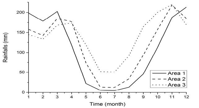
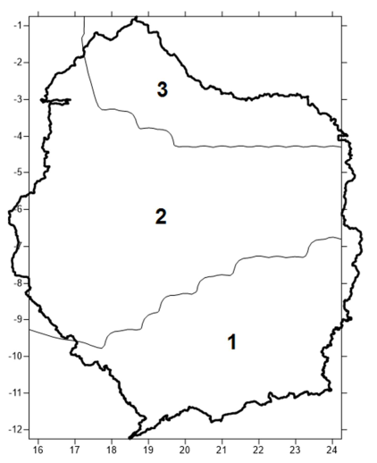
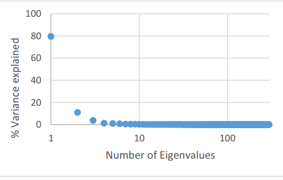
Only PC1 will be discussed as it contributes for 80 % of the rainfall variability in the Kasaï basin (figure 8).
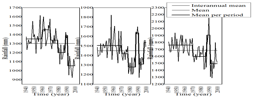
By Hubert segmentation, which gives us the year of different ruptures observed on the rainfall time series (Fig. 9), we can see that rains on the Kasaï basin are marked by fluctuations with a tendency on the one hand to the noticeable decline between 1970 and 1990, 1993 and 1999 and also an upward trend between 1960 and 1970 in area 1, 1990 and 1992.
The rain in area 1 presents five ruptures and therefore six times homogeneous rainfall:
wet phases 1940-1959; 1959-1969; 1970-1979; 1988-1990; dry phases 1980-1987; 1991-1999;
The rain in area 2 presents five ruptures and therefore six times homogeneous rainfall:
wet phases 1940-1969; 1988-1990; 1996-1999; dry phases 1970-1975; 1976-1987; 1991-1995;
The rain in area 3 presents three ruptures and therefore four times homogeneous rainfall:
wet phases 1940-1959; 1970-1979; dry phases 1959-1969; 1980-1987;
4.1 IDENTIFICATION OF VARIABILITY MODES
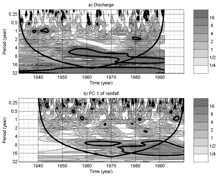
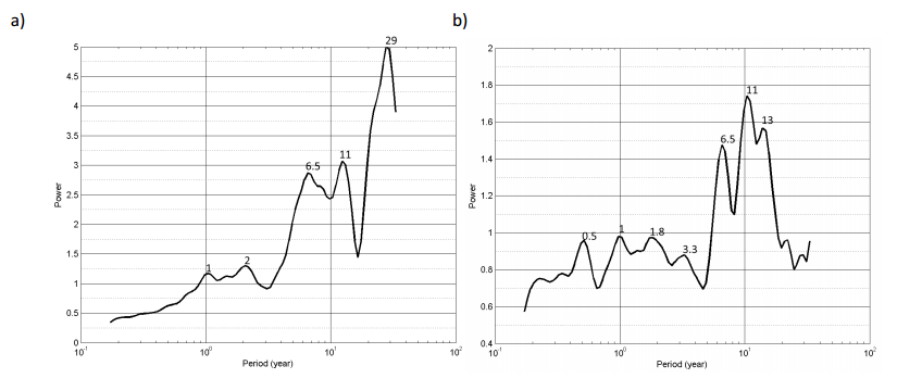
The wavelet analysis is used to study the frequency composition and visualize unsteady fluctuations of hydro variables so as to identify the main modes of variability of flows and precipitation in the basin of the Kasaï.
Table 1 shows the contribution of the energy bands in the discharge at Ilebo station and in rainfall in the Kasaï basin. The wavelet analysis of Kasaï flow shows a plurality of energy bands (Figure 10 and 11): A period of about 1 year mainly expressed A band of 2-8 years well localized:
- —
between 1953 and 1973 for both rainfalls and discharge;
- —
between 1973 and 1995 for rainfalls
A band of 8-16 years with a structure which begin around 1973 till 1999.
One can find a change point around 1970 (Figure 10 and 11) which is associated to low rainfalls and discharge.
| Discharge | Rainfall | |||
|---|---|---|---|---|
| Ilebo | Region 1 | Region 2 | Region 3 | |
| 0-1 year | 42% | 44% | 45% | 45% |
| 1-2 years | 34% | 35% | 30% | 25% |
| 2-8 years | 10% | 5% | 6% | 8% |
| 8-16 years | 6% | 3% | 4% | 6% |
4.2 COHERENCE BETWEEN RAINFALLS AND DISCHARGES
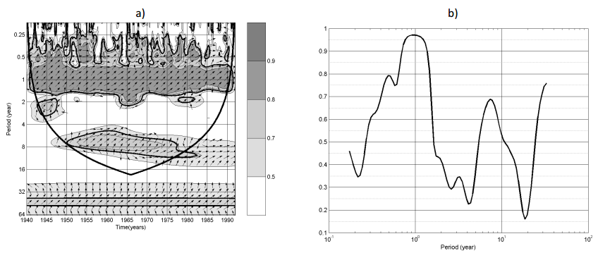
The discharge of Kasaï River at Ilebo station seems to be strongly related to the rainfalls with total coherence around 59.63%. Figure 12 attests that the coherence between discharge and rainfall in the Kasaï basin are essentially distributed across one year cycle and in 2-8 band (6.5 years).
4.3 RELATIONSHIP TO CLIMATE FORCING
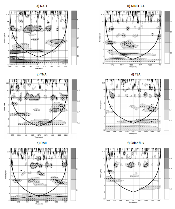
Some characteristic oscillations were next related to several well-known climate indices. The coherence wavelet analyses between discharge time series at Ilebo station, rainfalls (Figure 12) in the three area of Kasaï basin and climate index (NAO, NINO 3.4, TNA, TSA, DMI and Solar flux) show period of high coherence during some periods listed in table 3 and 4. Figure 13 and 14 also shows the characteristic periods of high wavelet coherence between discharge at Ilebo station, first principal component of rainfalls in Kasaï basin and selected climate indices.
| Observed scales | NAO | Nino 3.4 | TNA | TSA | DMI | Solar |
|---|---|---|---|---|---|---|
| 2-4 years | 1951-1955 | 1982-1987 | 1982-1987 | 1960-1969 | ||
| 1965-1971 | ||||||
| 1979-1990 | ||||||
| 4-8 years | 1955-1958 | 1932-1945 | 1950-1957 | 1948-1962 | ||
| 1952-1962 | 1980-1990 | |||||
| 8-16 years | 1950-1960 | 1948-1972 | 1967-1985 | 1967-1985 |

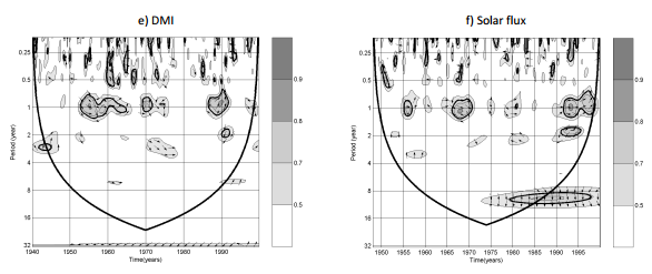
| Observed scales | NAO | Nino 3.4 | TNA | TSA | DMI | Solar flux |
|---|---|---|---|---|---|---|
| 2-4 years | 1955-1957 | 1957-1960 | 1940-1948 | 1956-1961 | ||
| 1964-1975 | 1967-1976 | 1951-1952 | ||||
| 1979-1984 | 1970-1978 | |||||
| 1982-1992 | ||||||
| 4-8 years | 1954-1967 | 1950-1967 | 1962-1972 | |||
| 8-16 years | 1975-1995 | 1967-1999 | 1957-1999 | 1972-1999 | 1980-1997 |
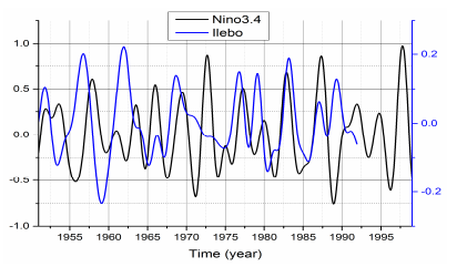
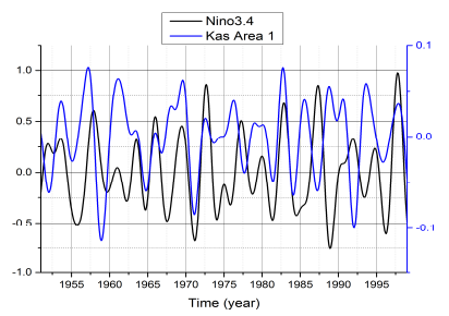

Figure 19 presents the relationships over the 2–8-yr band between the first principle component of the gridded rainfall over Kasaï basin and the Niño3.4 SST index.
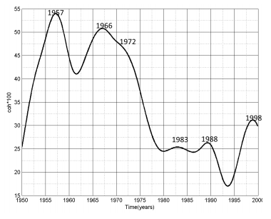
Mean percentage of wavelet coherence between discharge at Ilebo station or rainfall and some selected climate indices except Nino 3.4 index shows a weak nonlinear relationship (figure 20).

5 5 DISCUSSIONS AND CONCLUSION
We propose in this article a time-scale analysis of the river discharge fluctuations at Ilebo and rainfalls over the Kasaï basin. The two temporal discontinuities around 1970-1975 and 1990-1995 over figure 9 and 10 were also found in other studies [8], [20]. The wavelet coherence between discharges at Ilebo and rainfall over Kasaï River shows a high correlation in annual and the 2-8 year band –passed. Wavelet coherence between discharges at Ilebo and rainfall over Kasaï River and selected climate index confirm a less (figure 20) and nonlinear relationship between the hydrology of the Kasaï basin and the Pacific, Atlantic and Indian SST fluctuations. One can see covariability between rainfalls in the Kasaï basin and ENSO phenomenon, particularly at El Niño years [10] (Figure 15-19). The influence of teleconnections is low but their effects seem especially important having regard to the covariability observed with El Niño example. Further investigations should be conducted to understand the variability of the Kasaï river basin regime variability. What is the role of deforestation and of human activity and urbanization on water resource to availability?
ACKNOWLEDGMENTS
Thanks for the gridded rainfall data providers IRD and HydroSciences Montpellier, France. The wavelet software was provided by:
Torrence and Compo at http://atoc.colorado.edu/research/wavelets/
A. Grinsted at http://www.pol.ac.uk/home/research/waveletcoherence/
References
- [1] D. Backer, “La rivière kasaï entre kwamouth et port - francqui. l amélioration de ses conditions de navigabilité par balisage, signalisation et travaux dâaménagement,” bulletin des séances de l’Institut Royal Colonial Belge, vol. III, no. 1, pp. 252 – 278, 1932.
- [2] E. Devroey, Le Kasaï et son bassin hydrographique. Goemaere, 1939.
- [3] Ntombi and Kisangala, “Impact de la lithologie et de lâhydrométrie sur la navigabilité du kasaï en r. d. congo,” pp. 157–164, 2002.
- [4] Kisangala and Ntombi, “Estimation des réserves régulatrices et l’établissement de la courbe de tarissement du bassin versant du kasaè durant la période dâétiage à lâéchelle de lumbu,” Revue Congolaise des Sciences Nucléaires, vol. 26, no. 2, 2012.
- [5] [5] J.-F. Boyer, C. Dieulin, N. Rouche, A. Cres, E. Servat, J.-E. Paturel, and G. Mahe, “Sierem : an environmental information system for water resources,” IAHS publication, vol. 308, p. 19, 2006.
- [6] [6] N. Rouché, G. Mahé, S. Ardoin-Bardin, B. Brissaud, J.-f. Boyer, A. Crès, C. Dieulin, G. Bardin, G. Commelard, A. Dezetter, et al., “Constitution d’une grille de pluies mensuelles pour l’afrique (période 1900-2000),” Science et changements planétaires/Sécheresse, vol. 21, no. 4, pp. 336– 338, 2010.
- [7] G. Mahé, “Modulation annuelle et fluctuations interannuelles des précipitationscipitations sur le bassin-versant du congo,” pp. 13–26, 1995.
- [8] G. Mahé, Y. Lhote, J. C. Olivry, and G. Wotling, “Trends and discontinuities in regional rainfall of west and central africa : 1951 - 1989,” Hydrological Sciences Journal, vol. 46, no. 2, pp. 211 – 226, 2001.
- [9] J. W. Hurrell, “Decadal trends in the north atlantic oscillation : regional temperatures and precipitation,” Science, vol. 269, no. 5224, pp. 676–679, 1995.
- [10] K. E. Trenberth, “The definition of el nino,” Bulletin of the American Meteorological Society, vol. 78, no. 12, pp. 2771–2777, 1997
- [11] D. Enfield and E. Alfaro, “The dependence of caribbean rainfall on the interaction of the tropical atlantic and pacific oceans,” Journal of Climate, vol. 12, p. 2093â2103, 1999.
- [12] “Latest solar radio flux report from drao, penticton,â natural resources canada, 10 february 2016. [online]. available : http ://www.spaceweather.ca/solarflux/sx-4-en.php.”
- [13] K. Ashok, Z. Guan, and T. Yamagata, “Impact of the indian ocean dipole on the relationship between the indian monsoon rainfall and enso,” Geophysical Research Letters, vol. 28, no. 23, pp. 4499–4502, 2001.
- [14] S. Le Dien and J. Pagès, “Hierarchical multiple factor analysis : Application to the comparison of sensory profiles,” Food quality and preference, vol. 14, no. 5, pp. 397–403, 2003.
- [15] L. Lebart, A. Morineau, and K. M. Warwick, “Multivariate descriptive statistical analysis ; correspondence analysis and related techniques for large matrices,” 1984.
- [16] P. Hubert, J. P. Carbonnel, and A. Chaouche, “Segmentation des séries hydrométéorologiques : application à des séries de précipitations et de débits de l’afrique de l’ouest,” Journal of hydrology, vol. 110, no. 3, pp. 349–367, 1989.
- [17] C. Torrence and G. Compo, “A practical guide to wavelet analysis,” Bulletin of the American Meteorological Society, vol. 79, pp. 61 – 78, 1998.
- [18] M. Farge, “Wavelet transforms and their applications to turbulence,” Annual Review of Fluid Dynamics, vol. 24, pp. 395 – 457, 1992.
- [19] Y. Hao, G. Liu, H. Li, Z. Li, J. Zhao, and T.-C. J Yeh, “Investigation of karstic hydrological processes of niangziguan springs (north china) using wavelet analysis,” Hydrological Processes, vol. 26, no. 20, pp. 3062–3069, 2012.
- [20] [20] A. Laraque, G. Mahé, D. Orange, and B. Marieu, “Spatiotemporal variations in hydrological regimes within central africa during the xxth century,” Journal of Hydrology, vol. 245, no. 1, pp. 104–117, 2001.