跳到论文正文
W Papers独立论文阅读器 arXiv:1611.07237 论文正文 计算阅读时间 · 0%
引用这篇论文根据当前论文元数据生成,正式投稿前建议核对。


License: arXiv.org perpetual non-exclusive license
arXiv:1611.07237v2 [math.ST] 24 Nov 2016

Multivariate Intensity Estimation via Hyperbolic Wavelet Selection

Nathalie Akakpo Email address: nathalie.akakpo@upmc.fr Address: Laboratoire de Probabilités et Modèles Aléatoires (LPMA), UMR 7599
Université Pierre et Marie Curie (UPMC), Paris
Centre de Recherches Mathématiques (CRM), UMI 3457
Université de Montréal (UdeM)
Date: August 24, 2026
Abstract.

We propose a new statistical procedure able in some way to overcome the curse of dimensionality without structural assumptions on the function to estimate. It relies on a least-squares type penalized criterion and a new collection of models built from hyperbolic biorthogonal wavelet bases. We study its properties in a unifying intensity estimation framework, where an oracle-type inequality and adaptation to mixed smoothness are shown to hold. Besides, we describe an algorithm for implementing the estimator with a quite reasonable complexity.

Keywords: Hyperbolic wavelets; Biorthogonal wavelets; Mixed smoothness; Model selection; Density; Copula; Poisson process; Lévy process.

1. Introduction

Over the last decades, many wavelet procedures have been developed in various statistical frameworks. Yet, in multivariate settings, most of them are based on isotropic wavelet bases. These indeed have the advantage of being as easily tractable as their univariate counterparts since each isotropic wavelet is a tensor product of univariate wavelets coming from the same resolution level. Notable counterexamples are [19], [38] and [41], or [2] and [1]. They underline the usefulness of hyperbolic wavelet bases, where coordinatewise varying resolution levels are allowed, so as to recover a wider range of functions, and in particular functions with anisotropic smoothness.

Much attention has also been paid to the so-called curse of dimensionality. A common way to overcome this problem in Statistics is to impose structural assumptions on the function to estimate. In a regression framework, beyond the well-known additive and single-index models, we may cite the work of [25] who propose a spline-based method in an additive model with unknown link function, or the use of ANOVA-like decompositions in [28] or [16]. Besides, two landmark papers consider a general framework of composite functions, encompassing several classical structural assumptions: [29] propose a kernel-based procedure in the white noise framework, whereas [5] propose a general model selection procedure with a wide scope of applications. Finally, Lepski [31] (see also [47, 46]) consider density estimation with adaptation to a possibly multiplicative structure of the density. In the meanwhile, in the field of Approximation Theory and Numerical Analysis, a renewed interest in function spaces with dominating mixed smoothness has been growing (see for instance [20]), due to their tractability for multivariate integration for instance. Such spaces do not impose any structure, but only that the highest order derivative is a mixed derivative. Surprisingly, in the statistical literature, it seems that only the thresholding-type procedures of [38] and [12] deal with such spaces, either in the white noise framework or in a functional deconvolution model.

In order to fill this gap, this paper is devoted to a new statistical procedure based on wavelet selection from hyperbolic biorthogonal bases. We underline its universality by studying it in a general intensity estimation framework, encompassing many examples of interest such as density, copula density, Poisson intensity or Lévy jump intensity estimation. We first define a whole collection of linear subspaces, called models, generated by subsets of the dual hyperbolic basis, and a least-squares type criterion adapted to the norm induced by the primal hyperbolic basis. Then we describe a procedure to choose the best model from the data by using a penalized approach similar to [7]. Our procedure satisfies an oracle-type inequality provided the intensity to estimate is bounded. Besides, it reaches the minimax rate up to a constant factor, or up to a logarithmic factor, over a wide range of spaces with dominating mixed smoothness, and this rate is akin to the one we would obtain in a univariate framework. Notice that, contrary to [38] or [12], we allow for a greater variety of such spaces (of Sobolev, Hölder or Besov type smoothness) and also for spatially nonhomogeneous smoothness. For that purpose, we prove a key result from nonlinear approximation theory, in the spirit of [11], that may be of interest for other types of model selection procedures (see for instance [10, 4, 6]). Depending on the kind of intensity to estimate, different structural assumptions might make sense, some of which have been considered in [29], [5], [31], [47, 46], but not all. We explain in what respect these structural assumptions fall within the scope of estimation under dominating mixed smoothness. Yet, we emphasize that we do not need to impose any structural assumptions on the target function. Thus in some way our method is adaptive at the same time to many structures. Besides, it can be implemented with a computational complexity linear in the sample size, up to logarithmic factors.

The plan of the paper is as follows. In Section 2, we describe the general intensity estimation framework and several examples of interest. In Section 3, we define the so-called pyramidal wavelet models and a least-squares type criterion, and provide a detailed account of estimation on a given model. Section 4 is devoted to the choice of an adequate penalty so as to perform data-driven model selection. The optimality of the resulting procedure from the minimax point of view is then discussed in Section 5, under mixed smoothness assumptions. The algorithm for implementing our wavelet procedure and an illustrative example are given in Section 6. All proofs are postponed to Section 7. Let us end with some remark about the notation. Throughout the paper, C,C1,…C,C_{1},\ldots will stand for numerical constants, and C⁡(θ),C1​(θ),…C(\theta),C_{1}(\theta),\ldots for positive reals that only depend on some θ.\theta. Their values are allowed to change from line to line.

2. Framework and examples

2.1. General framework

Let d∈ℕ,d≥2,d\in\mathbb{N},d\geq 2, and Q=∏k=1d[ak,bk]Q=\prod_{k=1}^{d}\left[a_{k},b_{k}\right] be a given hyperrectangle in ℝd\mathbb{R}^{d} equipped with its Borel σ−\sigma-algebra ℬ⁡(Q)\mathcal{B}(Q) and the Lebesgue measure. We denote by 𝕃2​(Q)\mathbb{L}^{2}(Q) the space of square integrable functions on Q,Q, equipped with its usual norm

(1) ‖t‖=∫Qt2​(x)​𝑑x\|t\|=\sqrt{\int_{Q}t^{2}(x)\mathrm{d}x}

and scalar product ⟨.,.⟩.\langle.,.\rangle. In this article, we are interested in a nonnegative measure on ℬ⁡(Q)\mathcal{B}(Q) that admits a bounded density ss with respect to the Lebesgue measure, and our aim is to estimate that function ss over Q.Q. Given a probability space (Ω,ℰ,ℙ),(\Omega,\mathcal{E},\mathbb{P}), we assume that there exists some random measure MM defined on (Ω,ℰ,ℙ)(\Omega,\mathcal{E},\mathbb{P}), with values in the set of Borel measures on QQ such that, for all A∈ℬ⁡(Q),A\in\mathcal{B}(Q),

(2) 𝔼⁡[M⁡(A)]=⟨1​IA,s⟩.\mathbb{E}\left[M(A)\right]=\langle{1\kern-2.8889pt{}I}_{A},s\rangle.

By classical convergence theorems, this condition implies that, for all nonnegative or bounded measurable functions t,t,

(3) 𝔼⁡[∫Qt​𝑑M]=⟨t,s⟩.\mathbb{E}\left[\int_{Q}t\mathrm{d}M\right]=\langle t,s\rangle.

We assume that we observe some random measure M^,\widehat{M}, which is close enough to MM in a sense to be made precise later. When MM can be observed, we set of course M^=M.\widehat{M}=M.

2.2. Examples

Our general framework encompasses several special frameworks of interest, as we shall now show.

2.2.1. Example 1: density estimation.

Given n∈ℕ⋆,n\in\mathbb{N}^{\star}, we observe identically distributed random variables Y1,…,YnY_{1},\ldots,Y_{n} with common density ss with respect to the Lebesgue measure on Q=∏k=1d[ak,bk].Q=\prod_{k=1}^{d}\left[a_{k},b_{k}\right]. The observed empirical measure is then given by

M^​(A)=M⁡(A)=1n​∑i=1n1​IA​(Yi), for ​A∈ℬ⁡(Q),\widehat{M}(A)=M(A)=\frac{1}{n}\sum_{i=1}^{n}{1\kern-2.8889pt{}I}_{A}(Y_{i}),\text{ for }A\in\mathcal{B}(Q),

and obviously satisfies (2).

2.2.2. Example 2: copula density estimation.

Given n∈ℕ⋆,n\in\mathbb{N}^{\star}, we observe independent and identically distributed random variables X1,…,XnX_{1},\ldots,X_{n} with values in ℝd.\mathbb{R}^{d}. For i=1,…,ni=1,\ldots,n and j=1,…,d,j=1,\ldots,d, the jj-th coordinate Xi​jX_{ij} of XiX_{i} has continuous distribution function Fj.F_{j}. We recall that, from Sklar’s Theorem [50] (see also [37], for instance), there exists a unique distribution function CC on [0,1]d[0,1]^{d} with uniform marginals such that, for all (x1,…,xd)∈ℝd,(x_{1},\ldots,x_{d})\in\mathbb{R}^{d},

ℙ⁡(Xi​1≤x1,…,Xi​d≤xd)=C⁡(F1​(x1),…,Fd​(xd)).\mathbb{P}(X_{i1}\leq x_{1},\ldots,X_{id}\leq x_{d})=C(F_{1}(x_{1}),\ldots,F_{d}(x_{d})).

This function CC is called the copula of Xi​1,…,Xi​d.X_{i1},\ldots,X_{id}. We assume that it admits a density ss with respect to the Lebesgue measure on Q=[0,1]d.Q=[0,1]^{d}. Since CC is the joint distribution function of the Fj​(X1​j),j=1,…,d,F_{j}(X_{1j}),j=1,\ldots,d, a random measure satisfying (2) is given by

M⁡(A)=1n​∑i=1n1​IA​(F1​(Xi​1),…,Fd​(Xi​d)), for ​A∈ℬ⁡([0,1]d).M(A)=\frac{1}{n}\sum_{i=1}^{n}{1\kern-2.8889pt{}I}_{A}\left(F_{1}(X_{i1}),\ldots,F_{d}(X_{id})\right),\text{ for }A\in\mathcal{B}([0,1]^{d}).

As the marginal distributions FjF_{j} are usually unknown, we replace them by the empirical distribution functions F^n​j,\hat{F}_{nj}, where

F^n​j​(t)=1n​∑i=1n1​IXi​j≤t,\hat{F}_{nj}(t)=\frac{1}{n}\sum_{i=1}^{n}{1\kern-2.8889pt{}I}_{X_{ij}\leq t},

and define

M^​(A)=1n​∑i=1n1​IA​(F^n​1​(Xi​1),…,F^n​d​(Xi​d)), for ​A∈ℬ⁡([0,1]d).\widehat{M}(A)=\frac{1}{n}\sum_{i=1}^{n}{1\kern-2.8889pt{}I}_{A}\left(\hat{F}_{n1}(X_{i1}),\ldots,\hat{F}_{nd}(X_{id})\right),\text{ for }A\in\mathcal{B}([0,1]^{d}).

2.2.3. Example 3: Poisson intensity estimation.

Let us denote by Vold​(Q)\text{Vol}_{d}(Q) the Lebesgue measure of Q=∏k=1d[ak,bk].Q=\prod_{k=1}^{d}\left[a_{k},b_{k}\right]. We observe a Poisson process NN on QQ whose mean measure has intensity Vold​(Q)​s.\text{Vol}_{d}(Q)s. Otherwise said, for all finite family (Ak)1≤k≤K(A_{k})_{1\leq k\leq K} of disjoint measurable subsets of Q,Q, N⁡(A1),…,N⁡(AK)N(A_{1}),\ldots,N(A_{K}) are independent Poisson random variables with respective parameters Vold​(Q)​∫A1s,…,Vold​(Q)​∫AKs.\text{Vol}_{d}(Q)\int_{A_{1}}s,\ldots,\text{Vol}_{d}(Q)\int_{A_{K}}s. Therefore the empirical measure

M^​(A)=M⁡(A)=N⁡(A)Vold​(Q), for ​A∈ℬ⁡(Q),\widehat{M}(A)=M(A)=\frac{N(A)}{\text{Vol}_{d}(Q)},\text{ for }A\in\mathcal{B}(Q),

does satisfy (2). We do not assume ss to be constant throughout QQ so that the Poisson process may be nonhomogeneous.

2.2.4. Example 4: Lévy jump intensity estimation (continuous time).

Let TT be a fixed positive real, we observe on [0,T][0,T] a Lévy process 𝐗=(Xt)t≥0\mathbf{X}=(X_{t})_{t\geq 0} with values in ℝd.\mathbb{R}^{d}. Otherwise said, 𝐗\mathbf{X} is a process starting at 0,0, with stationary and independent increments, and which is continuous in probability with càdlàg trajectories (see for instance [8, 49, 15]). This process may have jumps, whose sizes are ruled by the so-called jump intensity measure or Lévy measure. An important example of such process is the compound Poisson process

Xt=∑i=1Ntξi,t≥0,X_{t}=\sum_{i=1}^{N_{t}}\xi_{i},t\geq 0,

where (Nt)t≥0(N_{t})_{t\geq 0} is a univariate homogeneous Poisson process, (ξi)i≥i(\xi_{i})_{i\geq i} are i.i.d. with values in ℝd\mathbb{R}^{d} and distribution ρ\rho with no mass at 0,0, and (Nt)t≥0(N_{t})_{t\geq 0} and (ξi)i≥i(\xi_{i})_{i\geq i} are independent. In this case, ρ\rho is also the Lévy measure of 𝐗.\mathbf{X}.

Here, we assume that the Lévy measure admits a density ff with respect to the Lebesgue measure on ℝd\{0}.\mathbb{R}^{d}\backslash\{0\}. Given some compact hyperrectangle Q=∏k=1d[ak,bk]⊂ℝd\{0},Q=\prod_{k=1}^{d}\left[a_{k},b_{k}\right]\subset\mathbb{R}^{d}\backslash\{0\}, our aim is to estimate the restriction ss of ff to Q.Q. For that purpose, we use the observed empirical measure

M^​(A)=M⁡(A)=1T​∬[0,T]×AN⁡(𝑑t,𝑑x), for ​A∈ℬ⁡(Q).\widehat{M}(A)=M(A)=\frac{1}{T}\iint\limits_{[0,T]\times A}N(\mathrm{d}t,\mathrm{d}x),\text{ for }A\in\mathcal{B}(Q).

A well-known property of Lévy processes states that the random measure NN defined for B∈ℬ([0,+∞)×ℝd\{0})B\in\mathcal{B}\left([0,+\infty)\times\mathbb{R}^{d}\backslash\{0\}\right) by

N(B)=♯{t>0/(t,Xt−Xt−)∈B}N(B)=\sharp\{t>0/(t,X_{t}-X_{t^{-}})\in B\}

is a Poisson process with mean measure

μ⁡(B)=∫∫Bf⁡(x)​𝑑t​𝑑x,\mu(B)=\int\int_{B}f(x)\mathrm{d}t\mathrm{d}x,

so that MM satisfies (2).

2.2.5. Example 5: Lévy jump intensity estimation (discrete time).

The framework is the same as in Example 4, except that (Xt)t≥0(X_{t})_{t\geq 0} is not observed. Given some time step Δ>0\Delta>0 and n∈ℕ⋆,n\in\mathbb{N}^{\star}, we only have at our disposal the random variables

Yi=Xi​Δ−X(i−1)​Δ,i=1,…n.Y_{i}=X_{i\Delta}-X_{(i-1)\Delta},i=1,\ldots n.

In order to estimate ss on Q,Q, we consider the random measure

M⁡(A)=1n​Δ​∬[0,n​Δ]×AN⁡(𝑑t,𝑑x), for ​A∈ℬ⁡(Q),M(A)=\frac{1}{n\Delta}\iint\limits_{[0,n\Delta]\times A}N(\mathrm{d}t,\mathrm{d}x),\text{ for }A\in\mathcal{B}(Q),

which is unobserved, and replaced for estimation purpose with

M^​(A)=1n​Δ​∑i=1n1​IA​(Yi), for ​A∈ℬ⁡(Q).\widehat{M}(A)=\frac{1}{n\Delta}\sum_{i=1}^{n}{1\kern-2.8889pt{}I}_{A}(Y_{i}),\text{ for }A\in\mathcal{B}(Q).

3. Estimation on a given pyramidal wavelet model

The first step of our estimation procedure relies on the definition of finite dimensional linear subspaces of 𝕃2​(Q),\mathbb{L}^{2}(Q), called models, generated by some finite families of biorthogonal wavelets. We only describe here models for Q=[0,1]d.Q=[0,1]^{d}. For a general hyperrectangle QQ, the adequate models can be deduced by translation and scaling. We then introduce a least-squares type contrast that allows to define an estimator of ss within a given wavelet model.

3.1. Wavelets on 𝕃2​([0,1])\mathbb{L}_{2}([0,1])

We shall first introduce a multiresolution analysis and a wavelet basis for 𝕃2​([0,1])\mathbb{L}_{2}([0,1]) satisfying the same general assumptions as in [27] and [26]. Concrete examples of wavelet bases satisfying those assumptions may be found in [14] and [17] for instance. In the sequel, we denote by κ\kappa some positive constant, that only depends on the choice of the bases. We fix the coarsest resolution level at j0∈ℕ.j_{0}\in\mathbb{N}. On the one hand, we assume that the scaling spaces

Vj=Vect​{ϕλ;λ∈Δj}​ and ​Vj⋆=Vect​{ϕλ⋆;λ∈Δj},j≥j0,V_{j}=\text{Vect}\{\phi_{\lambda};\lambda\in\Delta_{j}\}\text{ and }V^{\star}_{j}=\text{Vect}\{\phi^{\star}_{\lambda};\lambda\in\Delta_{j}\},j\geq j_{0},

satisfy the following hypotheses:

  1. S.i)S.i)

    (Riesz bases) For all j≥j0j\geq j_{0}, {ϕλ;λ∈Δj}\{\phi_{\lambda};\lambda\in\Delta_{j}\} are linearly independent functions from 𝕃2​([0,1])\mathbb{L}_{2}([0,1]), so are {ϕλ⋆;λ∈Δj}\{\phi^{\star}_{\lambda};\lambda\in\Delta_{j}\}, and they form Riesz bases of VjV_{j} and Vj⋆V^{\star}_{j}, i.e. ‖∑λ∈Δjaλ​ϕλ‖∼(∑λ∈Δjaλ2)1/2∼‖∑λ∈Δjaλ​ϕλ⋆‖.\left\|\sum_{\lambda\in\Delta_{j}}a_{\lambda}\phi_{\lambda}\right\|\sim\left(\sum_{\lambda\in\Delta_{j}}a^{2}_{\lambda}\right)^{1/2}\sim\left\|\sum_{\lambda\in\Delta_{j}}a_{\lambda}\phi^{\star}_{\lambda}\right\|.

  2. S.ii)S.ii)

    (Dimension) There exists some nonnegative integer BB such that, for all j≥j0j\geq j_{0}, dim(Vj)=dim(Vj⋆)=♯​Δj=2j+B.\dim(V_{j})=\dim(V^{\star}_{j})=\sharp\Delta_{j}=2^{j}+B.

  3. S.iii)S.iii)

    (Nesting) For all j≥j0j\geq j_{0}, Vj⊂Vj+1V_{j}\subset V_{j+1} and Vj⋆⊂Vj+1⋆.V^{\star}_{j}\subset V^{\star}_{j+1}.

  4. S.iv)S.iv)

    (Density) ∪j≥j0Vj¯=∪j≥j0V⋆j¯=𝕃2​([0,1])\overline{\cup_{j\geq j_{0}}V_{j}}=\overline{\cup_{j\geq j_{0}}V^{\star}_{j}}=\mathbb{L}_{2}([0,1]).

  5. S.v)S.v)

    (Biorthogonality) Let j≥j0j\geq j_{0}, for all λ,μ∈Δj\lambda,\mu\in\Delta_{j}, ⟨ϕλ,ϕμ⋆⟩=δλ,μ.\langle\phi_{\lambda},\phi^{\star}_{\mu}\rangle=\delta_{\lambda,\mu}.

  6. S.vi)S.vi)

    (Localization) Let j≥j0j\geq j_{0}, for all λ∈Δj\lambda\in\Delta_{j}, |Supp​(ϕλ)|∼|Supp​(ϕλ⋆)|∼2−j.|\text{Supp}(\phi_{\lambda})|\sim|\text{Supp}(\phi^{\star}_{\lambda})|\sim 2^{-j}.

  7. S.vii)S.vii)

    (Almost disjoint supports) For all j≥j0j\geq j_{0} and all λ∈Δj\lambda\in\Delta_{j},

    max(♯{μ∈Δj s.t. Supp(ϕλ)∩Supp(ϕμ)≠∅},♯{μ∈Δj s.t. Supp(ϕλ⋆)∩Supp(ϕμ⋆)≠∅})≤κ.\max\left(\sharp\{\mu\in\Delta_{j}\text{ s.t. }\text{Supp}(\phi_{\lambda})\cap\text{Supp}(\phi_{\mu})\neq\varnothing\},\sharp\{\mu\in\Delta_{j}\text{ s.t. }\text{Supp}(\phi^{\star}_{\lambda})\cap\text{Supp}(\phi^{\star}_{\mu})\neq\varnothing\}\right)\leq\kappa.
  8. S.viii)S.viii)

    (Norms) For all j≥j0j\geq j_{0} and all λ∈Δj\lambda\in\Delta_{j}, ‖ϕλ‖=‖ϕλ⋆‖=1\|\phi_{\lambda}\|=\|\phi^{\star}_{\lambda}\|=1 and max⁡(‖ϕλ‖∞,‖ϕλ⋆‖∞)≤κ​2j/2\max(\|\phi_{\lambda}\|_{\infty},\|\phi^{\star}_{\lambda}\|_{\infty})\leq\kappa 2^{j/2}.

  9. S.ix)S.ix)

    (Polynomial reproducibility) The primal scaling spaces are exact of order NN, i.e. for all j≥j0j\geq j_{0}, ΠN−1⊂Vj,\Pi_{N-1}\subset V_{j}, where ΠN−1\Pi_{N-1} is the set of all polynomial functions with degree ≤N−1\leq N-1 over [0,1].[0,1].

On the other hand, the wavelet spaces

Wj=Vect​{ψλ;λ∈∇j}​ and ​Wj⋆=Vect​{ψλ⋆;λ∈∇j},j≥j0+1,W_{j}=\text{Vect}\{\psi_{\lambda};\lambda\in\nabla_{j}\}\text{ and }W^{\star}_{j}=\text{Vect}\{\psi^{\star}_{\lambda};\lambda\in\nabla_{j}\},j\geq j_{0}+1,

fulfill the following conditions:

  1. W.i)W.i)

    (Riesz bases) The functions {ψλ;λ∈∪j≥j0+1∇j}\{\psi_{\lambda};\lambda\in\cup_{j\geq j_{0}+1}\nabla_{j}\} are linearly independent. Together with the {ϕλ;λ∈Δj0}\{\phi_{\lambda};\lambda\in\Delta_{j_{0}}\}, they form a Riesz basis for 𝕃2​([0,1])\mathbb{L}_{2}([0,1]). The same holds for the ψ⋆\psi^{\star} and the ϕ⋆\phi^{\star}.

  2. W.ii)W.ii)

    (Orthogonality) For all j≥j0j\geq j_{0}, Vj+1=Vj⊕Wj+1V_{j+1}=V_{j}\oplus W_{j+1} and Vj+1⋆=Vj⋆⊕Wj+1⋆V^{\star}_{j+1}=V^{\star}_{j}\oplus W^{\star}_{j+1}, with Vj⟂Wj+1⋆V_{j}\perp W^{\star}_{j+1} and Vj⋆⟂Wj+1.V^{\star}_{j}\perp W_{j+1}.

  3. W.iii)W.iii)

    (Biorthogonality) Let j≥j0j\geq j_{0}, for all λ,μ∈∇j+1\lambda,\mu\in\nabla_{j+1}, ⟨ψλ,ψμ⋆⟩=δλ,μ.\langle\psi_{\lambda},\psi^{\star}_{\mu}\rangle=\delta_{\lambda,\mu}.

  4. W.iv)W.iv)

    (Localization) Let j≥j0j\geq j_{0}, for all λ∈∇j+1\lambda\in\nabla_{j+1}, |Supp​(ψλ)|∼|Supp​(ψλ⋆)|∼2−j.|\text{Supp}(\psi_{\lambda})|\sim|\text{Supp}(\psi^{\star}_{\lambda})|\sim 2^{-j}.

  5. W.v)W.v)

    (Almost disjoint supports) For all j≥j0j\geq j_{0} and all λ∈∇j+1\lambda\in\nabla_{j+1},

    max(♯{μ∈∇j+1 s.t. Supp(ψλ)∩Supp(ψμ)≠∅},♯{μ∈∇j+1 s.t. Supp(ψλ⋆)∩Supp(ψμ⋆)≠∅})≤κ.\max\left(\sharp\{\mu\in\nabla_{j+1}\text{ s.t. }\text{Supp}(\psi_{\lambda})\cap\text{Supp}(\psi_{\mu})\neq\varnothing\},\sharp\{\mu\in\nabla_{j+1}\text{ s.t. }\text{Supp}(\psi^{\star}_{\lambda})\cap\text{Supp}(\psi^{\star}_{\mu})\neq\varnothing\}\right)\leq\kappa.
  6. W.vi)W.vi)

    (Norms) For all j≥j0j\geq j_{0} and all λ∈∇j+1\lambda\in\nabla_{j+1}, ‖ψλ‖=‖ψλ⋆‖=1\|\psi_{\lambda}\|=\|\psi^{\star}_{\lambda}\|=1 and max⁡(‖ψλ‖∞,‖ψλ⋆‖∞)≤κ​2j/2\max(\|\psi_{\lambda}\|_{\infty},\|\psi^{\star}_{\lambda}\|_{\infty})\leq\kappa 2^{j/2}.

  7. W.vii)W.vii)

    (Fast Wavelet Transform) Let j≥j0j\geq j_{0}, for all λ∈∇j+1\lambda\in\nabla_{j+1},

    ♯⁡{μ∈Δj+1|⟨ψλ,ϕμ⟩≠0}≤κ\sharp\{\mu\in\Delta_{j+1}|\langle\psi_{\lambda},\phi_{\mu}\rangle\neq 0\}\leq\kappa

    and for all μ∈Δj+1\mu\in\Delta_{j+1}

    |⟨ψλ,ϕμ⟩|≤κ.|\langle\psi_{\lambda},\phi_{\mu}\rangle|\leq\kappa.

    The same holds for the ψλ⋆\psi^{\star}_{\lambda} and the ϕλ⋆.\phi^{\star}_{\lambda}.

Remarks:

  • •

    These properties imply that any function f∈𝕃2​([0,1])f\in\mathbb{L}_{2}([0,1]) may be decomposed as

    (4) f=∑λ∈Δj0⟨f,ϕλ⟩​ϕλ⋆+∑j≥j0+1∑λ∈∇j⟨f,ψλ⟩​ψλ⋆.f=\sum_{\lambda\in\Delta_{j_{0}}}\langle f,\phi_{\lambda}\rangle\phi^{\star}_{\lambda}+\sum_{j\geq j_{0}+1}\sum_{\lambda\in\nabla_{j}}\langle f,\psi_{\lambda}\rangle\psi^{\star}_{\lambda}.
  • •

    Properties S.ii)S.ii) and W.ii)W.ii) imply that dim(Wj+1)=2j.\dim(W_{j+1})=2^{j}.

  • •

    Property W.vii)W.vii) means in particular that, for each resolution level jj, any wavelet can be represented as a linear combination of scaling functions from the same resolution level with a number of components bounded independently of the level as well as the amplitude of the coefficients.

As is well known, contrary to orthogonal bases, biorthogonal bases allow for both symmetric and smooth wavelets. Besides, properties of dual biorthogonal bases are usually not the same. Usually, in decomposition (4), the analysis wavelets ϕλ\phi_{\lambda} and ψλ\psi_{\lambda} are the one with most null moments, whereas the synthesis wavelets ϕλ⋆\phi^{\star}_{\lambda} and ψλ⋆\psi^{\star}_{\lambda} are the one with greatest smoothness. Yet, we may sometimes need the following smoothness assumptions on the analysis wavelets (not very restrictive in practice), only to bound residual terms due to the replacement of MM with M^.\widehat{M}.

Assumption (L). For all λ∈Δj0\lambda\in\Delta_{j_{0}}, for all j≥j0j\geq j_{0} and all μ∈∇j+1,\mu\in\nabla_{j+1}, ϕλ\phi_{\lambda} and ψμ\psi_{\mu} are Lipschitz functions with Lipschitz norms satisfying ‖ϕλ‖L≤κ​23​j0/2\|\phi_{\lambda}\|_{L}\leq\kappa 2^{3j_{0}/2} and ‖ψμ‖L≤κ​23​j/2.\|\psi_{\mu}\|_{L}\leq\kappa 2^{3j/2}.

We still refer to [14] and [17] for examples of wavelet bases satisfying this additional assumption.

3.2. Hyperbolic wavelet basis on 𝕃2​([0,1]d)\mathbb{L}_{2}([0,1]^{d})

In the sequel, for ease of notation, we set ℕj0={j∈ℕ,j≥j0},\mathbb{N}_{j_{0}}=\{j\in\mathbb{N},j\geq j_{0}\}, ∇j0=Δj0\nabla_{j_{0}}=\Delta_{j_{0}}, Wj0=Vj0W_{j_{0}}=V_{j_{0}} and Wj0⋆=Vj0⋆,W^{\star}_{j_{0}}=V^{\star}_{j_{0}}, and for λ∈∇j0\lambda\in\nabla_{j_{0}}, ψλ=ϕλ\psi_{\lambda}=\phi_{\lambda} and ψλ⋆=ϕλ⋆.\psi^{\star}_{\lambda}=\phi^{\star}_{\lambda}. Given a biorthogonal basis of 𝕃2​([0,1])\mathbb{L}_{2}([0,1]) chosen according to 3.1, we deduce biorthogonal wavelets of 𝕃2​([0,1]d)\mathbb{L}_{2}([0,1]^{d}) by tensor product. More precisely, for 𝒋=(j1,…,jd)∈ℕj0d\bm{j}=(j_{1},\ldots,j_{d})\in\mathbb{N}_{j_{0}}^{d}, we set ∇𝒋=∇j1×…×∇jd\bm{\nabla_{j}}=\nabla_{j_{1}}\times\ldots\times\nabla_{j_{d}} and for all 𝝀=(λ1,…,λd)∈∇𝒋\bm{\lambda}=(\lambda_{1},\ldots,\lambda_{d})\in\bm{\nabla_{j}}, we define Ψ𝝀​(x1,…,xd)=ψλ1​(x1)​…​ψλd​(xd)\Psi_{\bm{\lambda}}(x_{1},\ldots,x_{d})=\psi_{\lambda_{1}}(x_{1})\ldots\psi_{\lambda_{d}}(x_{d}) and Ψ𝝀⋆​(x1,…,xd)=ψλ1⋆​(x1)​…​ψλd⋆​(xd).\Psi^{\star}_{\bm{\lambda}}(x_{1},\ldots,x_{d})=\psi^{\star}_{\lambda_{1}}(x_{1})\ldots\psi^{\star}_{\lambda_{d}}(x_{d}). Contrary to most statistical works based on wavelets, we thus allow for tensor products of univariate wavelets coming from different resolution levels j1,…,jd.j_{1},\ldots,j_{d}. Writing Λ=∪𝒋∈ℕj0d∇𝒋,\Lambda=\cup_{{\bm{j}}\in\mathbb{N}_{j_{0}}^{d}}\bm{\nabla}_{\bm{j}}, the families {Ψ𝝀;𝝀∈Λ}\{\Psi_{\bm{\lambda}};\bm{\lambda}\in\Lambda\} and {Ψ𝝀⋆;𝝀∈Λ}\{\Psi^{\star}_{\bm{\lambda}};\bm{\lambda}\in\Lambda\} define biorthogonal bases of 𝕃2​([0,1]d)\mathbb{L}_{2}([0,1]^{d}) called biorthogonal hyperbolic bases. Indeed,

𝕃2​([0,1]d)=∪j≥j0Vj⊗…⊗Vj¯,\mathbb{L}_{2}([0,1]^{d})=\overline{\cup_{j\geq j_{0}}V_{j}\otimes\ldots\otimes V_{j}},

and for all j≥j0,j\geq j_{0},

Vj⊗…⊗Vj\displaystyle V_{j}\otimes\ldots\otimes V_{j} =(Wj0⊕Wj0+1⊕…⊕Wj)⊗…⊗(Wj0⊕Wj0+1⊕…⊕Wj)\displaystyle=(W_{j_{0}}\oplus W_{j_{0}+1}\oplus\ldots\oplus W_{j})\otimes\ldots\otimes(W_{j_{0}}\oplus W_{j_{0}+1}\oplus\ldots\oplus W_{j})
=⊕j0≤k1,…,kd≤j​Wk1⊗…⊗Wkd.\displaystyle=\underset{j_{0}\leq k_{1},\ldots,k_{d}\leq j}{\oplus}W_{k_{1}}\otimes\ldots\otimes W_{k_{d}}.

In the same way,

𝕃2​([0,1]d)=∪j≥j0⊕j0≤k1,…,kd≤jW⋆k1⊗…⊗W⋆kd¯.\mathbb{L}_{2}([0,1]^{d})=\overline{\cup_{j\geq j_{0}}\underset{j_{0}\leq k_{1},\ldots,k_{d}\leq j}{\oplus}W^{\star}_{k_{1}}\otimes\ldots\otimes W^{\star}_{k_{d}}}.

Besides, they induce on 𝕃2​([0,1]d)\mathbb{L}_{2}([0,1]^{d}) the norms

(5) ‖t‖𝚿=∑𝝀∈Λ⟨t,Ψ𝝀⟩2​ and ​‖t‖𝚿⋆=∑𝝀∈Λ⟨t,Ψ𝝀⋆⟩2,\|t\|_{\bm{\Psi}}=\sqrt{\sum_{\bm{\lambda}\in\Lambda}\langle t,\Psi_{\bm{\lambda}}\rangle^{2}}\text{ and }\|t\|_{\bm{\Psi}^{\star}}=\sqrt{\sum_{\bm{\lambda}\in\Lambda}\langle t,\Psi^{\star}_{\bm{\lambda}}\rangle^{2}},

which are both equivalent to ∥.∥,\|.\|, with equality when the wavelet basis is orthogonal. It should be noticed that the scalar product derived from ∥.∥𝚿,\|.\|_{\bm{\Psi}}, for instance, is

(6) ⟨t,u⟩𝚿=∑𝝀∈Λ⟨t,Ψ𝝀⟩​⟨u,Ψ𝝀⟩.\langle t,u\rangle_{\bm{\Psi}}=\sum_{\bm{\lambda}\in\Lambda}\langle t,\Psi_{\bm{\lambda}}\rangle\langle u,\Psi_{\bm{\lambda}}\rangle.

3.3. Pyramidal models

A wavelet basis in dimension 1 has a natural pyramidal structure when the wavelets are grouped according to their resolution level. A hyperbolic basis too, provided we define a proper notion of resolution level that takes into account anisotropy: for a wavelet Ψ𝝀\Psi_{\bm{\lambda}} or Ψ𝝀⋆\Psi^{\star}_{\bm{\lambda}} with 𝝀∈∇𝒋,\bm{\lambda}\in\bm{\nabla}_{\bm{j}}, we define the global resolution level as |𝒋|:=j1+…+jd.|\bm{j}|:=j_{1}+\ldots+j_{d}. Thus, the supports of all wavelets corresponding to a given global resolution level ℓ∈ℕd​j0\ell\in\mathbb{N}_{dj_{0}} have a volume of roughly 2−ℓ2^{-\ell} but exhibit very different shapes. For all ℓ∈ℕd​j0,\ell\in\mathbb{N}_{dj_{0}}, we define 𝑱ℓ={𝒋∈ℕj0d/|𝒋|=ℓ},\bm{J}_{\ell}=\{\bm{j}\in\mathbb{N}_{j_{0}}^{d}/|\bm{j}|=\ell\}, and U∇(ℓ)=∪𝒋∈𝑱ℓ∇𝒋U\bm{\nabla}(\ell)=\cup_{\bm{j}\in\bm{J}_{\ell}}\bm{\nabla}_{\bm{j}} the index set for dd-variate wavelets at resolution level ℓ\ell.

Given some maximal resolution level L∙∈ℕd​j0L_{\bullet}\in\mathbb{N}_{dj_{0}}, we define, for all ℓ1∈{d​j0+1,…,L∙+1}\ell_{1}\in\{dj_{0}+1,\ldots,L_{\bullet}+1\}, the family ℳℓ1𝒫\mathcal{M}^{\mathcal{P}}_{\ell_{1}} of all sets mm of the form

m=(⋃ℓ=d​j0ℓ1−1U∇(ℓ))∪(⋃k=0L∙−ℓ1m(ℓ1+k)),m=\left(\bigcup_{\ell=dj_{0}}^{\ell_{1}-1}U\bm{\nabla}(\ell)\right)\cup\left(\bigcup_{k=0}^{L_{\bullet}-\ell_{1}}m(\ell_{1}+k)\right),

where, for all 0≤k≤L∙−ℓ10\leq k\leq L_{\bullet}-\ell_{1}, m⁡(ℓ1+k)m(\ell_{1}+k) may be any subset of U∇(ℓ1+k)U\bm{\nabla}(\ell_{1}+k) with N⁡(ℓ1,k)N(\ell_{1},k) elements. Typically, N⁡(ℓ1,k)N(\ell_{1},k) will be chosen so as to impose some sparsity: it is expected to be smaller than the total number of wavelets at level ℓ1+k\ell_{1}+k and to decrease when the resolution level increases. An adequate choice of N⁡(ℓ1,k)N(\ell_{1},k) will be proposed in Proposition 4. Thus, choosing a set in ℳℓ1𝒫\mathcal{M}^{\mathcal{P}}_{\ell_{1}} amounts to keep all hyperbolic wavelets at level at most ℓ1−1,\ell_{1}-1, but only a few at deeper levels. We set ℳ𝒫=∪ℓ1=d​j0+1L∙+1ℳ𝒫ℓ1\mathcal{M}^{\mathcal{P}}=\cup_{\ell_{1}=dj_{0}+1}^{L_{\bullet}+1}\mathcal{M}^{\mathcal{P}}_{\ell_{1}} and define a pyramidal model as any finite dimensional subspace of the form

Sm⋆=Vect​{Ψ𝝀⋆;𝝀∈m}, for ​m∈ℳ𝒫.S^{\star}_{m}=\text{Vect}\{\Psi^{\star}_{\bm{\lambda}};\bm{\lambda}\in m\},\text{ for }m\in\mathcal{M}^{\mathcal{P}}.

We denote by DmD_{m} the dimension of Sm⋆.S^{\star}_{m}. Setting m∙=⋃ℓ=d​j0L∙U∇(ℓ),m_{\bullet}=\bigcup_{\ell=dj_{0}}^{L_{\bullet}}U\bm{\nabla}(\ell), we can see that all pyramidal models are included in Sm∙⋆.S^{\star}_{m_{\bullet}}.

3.4. Least-squares type estimator on a pyramidal model

Let us fix some model m∈ℳ𝒫.m\in\mathcal{M}^{\mathcal{P}}. If the random measure MM is observed, then we can build a least-squares type estimator sˇm⋆\check{s}_{m}^{\star} for ss with values in Sm⋆S^{\star}_{m} and associated with the norm ∥.∥𝚿\|.\|_{\bm{\Psi}} defined by (5). Indeed, setting

γ⁡(t)=‖t‖𝚿2−2​∑𝝀∈Λ⟨t,Ψ𝝀⟩​βˇ𝝀,\gamma(t)=\|t\|_{\bm{\Psi}}^{2}-2\sum_{\bm{\lambda}\in\Lambda}\langle t,\Psi_{\bm{\lambda}}\rangle\check{\beta}_{\bm{\lambda}},

where

βˇ𝝀=∫QΨ𝝀​𝑑M,\check{\beta}_{\bm{\lambda}}=\int_{Q}\Psi_{\bm{\lambda}}\mathrm{d}M,

we deduce from (3) that ss minimizes over t∈𝕃2​(Q)t\in\mathbb{L}^{2}(Q)

‖s−t‖𝚿2−‖s‖𝚿2=‖t‖𝚿2−2​∑𝝀∈Λ⟨t,Ψ𝝀⟩​⟨s,Ψ𝝀⟩=𝔼⁡[γ⁡(t)],\displaystyle\|s-t\|^{2}_{\bm{\Psi}}-\|s\|^{2}_{\bm{\Psi}}=\|t\|^{2}_{\bm{\Psi}}-2\sum_{\bm{\lambda}\in\Lambda}\langle t,\Psi_{\bm{\lambda}}\rangle\langle s,\Psi_{\bm{\lambda}}\rangle=\mathbb{E}[\gamma(t)],

so we introduce

sˇm⋆=argmin t∈Sm⋆​γ​(t).\check{s}^{\star}_{m}=\underset{t\in S^{\star}_{m}}{\text{argmin }}\gamma(t).

For all sequences of reals (α𝝀)𝝀∈m,(\alpha_{\bm{\lambda}})_{\bm{\lambda}\in m},

(7) γ⁡(∑𝝀∈mα𝝀​Ψ𝝀⋆)=∑𝝀∈m(α𝝀−βˇ𝝀)2−∑𝝀∈mβˇ𝝀2,\gamma\left(\sum_{\bm{\lambda}\in m}\alpha_{\bm{\lambda}}\Psi^{\star}_{\bm{\lambda}}\right)=\sum_{\bm{\lambda}\in m}\left(\alpha_{\bm{\lambda}}-\check{\beta}_{\bm{\lambda}}\right)^{2}-\sum_{\bm{\lambda}\in m}\check{\beta}_{\bm{\lambda}}^{2},

hence

sˇm⋆=∑𝝀∈mβˇ𝝀​Ψ𝝀⋆.\check{s}^{\star}_{m}=\sum_{\bm{\lambda}\in m}\check{\beta}_{\bm{\lambda}}\Psi^{\star}_{\bm{\lambda}}.

Since we only observe the random measure M^,\widehat{M}, we consider the pseudo-least-squares contrast

γ^​(t)=‖t‖𝚿2−2​∑𝝀∈Λ⟨t,Ψ𝝀⟩​β^𝝀,\widehat{\gamma}(t)=\|t\|_{\bm{\Psi}}^{2}-2\sum_{\bm{\lambda}\in\Lambda}\langle t,\Psi_{\bm{\lambda}}\rangle{\widehat{\beta}_{\bm{\lambda}}},

where

β^𝝀=∫QΨ𝝀​𝑑M^,\widehat{\beta}_{\bm{\lambda}}=\int_{Q}\Psi_{\bm{\lambda}}\mathrm{d}\widehat{M},

and we define the best estimator of ss within Sm⋆S^{\star}_{m} as

s^m⋆=argmin t∈Sm⋆​γ^​(t)=∑𝝀∈mβ^𝝀​Ψ𝝀⋆.\widehat{s}^{\star}_{m}=\underset{t\in S^{\star}_{m}}{\text{argmin }}\widehat{\gamma}(t)=\sum_{\bm{\lambda}\in m}\widehat{\beta}_{\bm{\lambda}}\Psi^{\star}_{\bm{\lambda}}.

3.5. Quadratic risk on a pyramidal model

Let us introduce the orthogonal projection of ss on Sm⋆S^{\star}_{m} for the norm ∥.∥𝚿,\|.\|_{\bm{\Psi}}, that is

sm⋆=∑𝝀∈mβ𝝀​Ψ𝝀⋆,s^{\star}_{m}=\sum_{\bm{\lambda}\in m}\beta_{\bm{\lambda}}\Psi^{\star}_{\bm{\lambda}},

where

β𝝀=⟨Ψ𝝀,s⟩.\beta_{\bm{\lambda}}=\langle\Psi_{\bm{\lambda}},s\rangle.

It follows from (3) that βˇ𝝀\check{\beta}_{\bm{\lambda}} is an unbiased estimator for β𝝀,\beta_{\bm{\lambda}}, so that sˇm⋆\check{s}^{\star}_{m} is an unbiased estimator for sm⋆.s^{\star}_{m}. Thanks to Pythagoras’ equality, we recover for sˇm⋆\check{s}^{\star}_{m} the usual decomposition

(8) 𝔼⁡[‖s−sˇm⋆‖𝚿2]=‖s−sm⋆‖𝚿2+∑𝝀∈mVar​(βˇ𝝀),\mathbb{E}\left[\|s-\check{s}^{\star}_{m}\|^{2}_{\bm{\Psi}}\right]=\|s-s^{\star}_{m}\|^{2}_{\bm{\Psi}}+\sum_{\bm{\lambda}\in m}\text{{Var}}(\check{\beta}_{\bm{\lambda}}),

where the first term is a bias term or approximation error and the second term is a variance term or estimation error. When only M^\widehat{M} is observed, combining the triangle inequality, the basic inequality (14) and (8) easily provides at least an upper-bound akin to (8), up to a residual term.

Proposition 1.

For all θ>0,\theta>0,

𝔼⁡[‖s−s^m⋆‖𝚿2]≤(1+θ)​(‖s−sm⋆‖𝚿2+∑𝝀∈mVar​(βˇ𝝀))+(1+1/θ)​𝔼​[‖sˇm⋆−s^m⋆‖𝚿2].\mathbb{E}\left[\|s-\hat{s}^{\star}_{m}\|^{2}_{\bm{\Psi}}\right]\leq(1+\theta)\left(\|s-s^{\star}_{m}\|^{2}_{\bm{\Psi}}+\sum_{\bm{\lambda}\in m}\text{{Var}}(\check{\beta}_{\bm{\lambda}})\right)+(1+1/\theta)\mathbb{E}\left[\|\check{s}^{\star}_{m}-\hat{s}^{\star}_{m}\|^{2}_{\bm{\Psi}}\right].

When M^=M,\widehat{M}=M, θ\theta can be taken equal to 0 and equality holds.

In all the examples introduced in Section 2.2, we shall verify that the quadratic risks satisfies, for all θ>0,\theta>0,

(9) 𝔼⁡[‖s−s^m⋆‖𝚿2]≤c1​‖s−sm⋆‖𝚿2+c2​‖s‖∞​Dmn¯+r1​(n¯),\mathbb{E}\left[\|s-\hat{s}^{\star}_{m}\|^{2}_{\bm{\Psi}}\right]\leq c_{1}\|s-s^{\star}_{m}\|^{2}_{\bm{\Psi}}+c_{2}\frac{\|s\|_{\infty}D_{m}}{\bar{n}}+r_{1}(\bar{n}),

where n¯\bar{n} describes the amount of available data, and the residual term r1​(n¯)r_{1}(\bar{n}) does not weigh too much upon the estimation rate.

3.5.1. Example 1: density estimation (continued).

In this framework, the empirical coefficients are of the form

βˇ𝝀=1n​∑i=1nΨ𝝀​(Yi).\check{\beta}_{\bm{\lambda}}=\frac{1}{n}\sum_{i=1}^{n}\Psi_{\bm{\lambda}}(Y_{i}).

As the wavelets are normalized and ss is bounded,

Var​(βˇ𝝀)≤1n​∫QΨ𝝀2​(x)​s​(x)​𝑑x≤‖s‖∞n,\text{{Var}}(\check{\beta}_{\bm{\lambda}})\leq\frac{1}{n}\int_{Q}\Psi^{2}_{\bm{\lambda}}(x)s(x)\mathrm{d}x\leq\frac{\|s\|_{\infty}}{n},

so

𝔼⁡[‖s−s^m⋆‖𝚿2]≤‖s−sm⋆‖𝚿2+‖s‖∞​Dmn.\mathbb{E}\left[\|s-\hat{s}^{\star}_{m}\|^{2}_{\bm{\Psi}}\right]\leq\|s-s^{\star}_{m}\|^{2}_{\bm{\Psi}}+\frac{\|s\|_{\infty}D_{m}}{n}.

Hence (9) is satisfied for instance with n¯=n,\bar{n}=n, c1=c2=1,r1​(n)=0.c_{1}=c_{2}=1,r_{1}(n)=0.

3.5.2. Example 2: copula density estimation (continued).

In this case,

βˇ𝝀=1n​∑i=1nΨ𝝀​(F1​(Xi​1),…,Fd​(Xi​d)),\check{\beta}_{\bm{\lambda}}=\frac{1}{n}\sum_{i=1}^{n}\Psi_{\bm{\lambda}}\left(F_{1}(X_{i1}),\ldots,F_{d}(X_{id})\right),

while

β^𝝀=1n​∑i=1nΨ𝝀​(F^n​1​(Xi​1),…,F^n​d​(Xi​d)).\widehat{\beta}_{\bm{\lambda}}=\frac{1}{n}\sum_{i=1}^{n}\Psi_{\bm{\lambda}}\left(\hat{F}_{n1}(X_{i1}),\ldots,\hat{F}_{nd}(X_{id})\right).

As in Example 1, Var​(βˇ𝝀)≤‖s‖∞/n.\text{{Var}}(\check{\beta}_{\bm{\lambda}})\leq\|s\|_{\infty}/n. Besides we prove in Section 7.1 the following upper-bound for the residual terms.

Proposition 2.

Under Assumption (L), for all m∈ℳ𝒫,m\in\mathcal{M}^{\mathcal{P}},

𝔼⁡[‖sˇm⋆−s^m⋆‖2]≤C⁡(κ,d)​L∙d−1​24​L∙​log⁡(n)/n.\mathbb{E}[\|\check{s}^{\star}_{m}-\hat{s}^{\star}_{m}\|^{2}]\leq C(\kappa,d)L^{d-1}_{\bullet}2^{4L_{\bullet}}\log(n)/n.

Hence choosing n¯=n,\bar{n}=n, 24​L∙=n/log⁡(n),2^{4L_{\bullet}}=\sqrt{n}/\log(n), c1=c2=2,c_{1}=c_{2}=2, and r1​(n)=C⁡(κ,d)​log⁡(n)d−1/nr_{1}(n)=C(\kappa,d)\log(n)^{d-1}/\sqrt{n} yields (9).

3.5.3. Example 3: Poisson intensity estimation (continued).

In this case,

βˇ𝝀=1Vold​(Q)​∫QΨ𝝀​(x)​N​(𝑑x).\check{\beta}_{\bm{\lambda}}=\frac{1}{\text{Vol}_{d}(Q)}\int_{Q}\Psi_{\bm{\lambda}}(x)N(\mathrm{d}x).

From Campbell’s formula,

Var​(βˇ𝝀)=1Vold​(Q)​∫QΨ𝝀2​(x)​s​(x)​𝑑x\text{{Var}}(\check{\beta}_{\bm{\lambda}})=\frac{1}{\text{Vol}_{d}(Q)}\int_{Q}\Psi^{2}_{\bm{\lambda}}(x)s(x)\mathrm{d}x

so

𝔼⁡[‖s−s^m⋆‖𝚿2]≤‖s−sm⋆‖𝚿2+‖s‖∞​Dmn¯,\mathbb{E}\left[\|s-\hat{s}^{\star}_{m}\|^{2}_{\bm{\Psi}}\right]\leq\|s-s^{\star}_{m}\|^{2}_{\bm{\Psi}}+\frac{\|s\|_{\infty}D_{m}}{\bar{n}},

with n¯=Vold​(Q).\bar{n}=\text{Vol}_{d}(Q).

3.5.4. Example 4: Lévy jump intensity estimation with continuous time observations (continued).

In this case,

βˇ𝝀=1T​∬[0,T]×QΨ𝝀​(x)​N​(𝑑t,𝑑x).\check{\beta}_{\bm{\lambda}}=\frac{1}{T}\iint\limits_{[0,T]\times Q}\Psi_{\bm{\lambda}}(x)N(\mathrm{d}t,\mathrm{d}x).

From Campbell’s formula again,

Var​(βˇ𝝀)=1T2​∬[0,T]×QΨ𝝀2​(x)​s​(x)​𝑑t​𝑑x\text{{Var}}(\check{\beta}_{\bm{\lambda}})=\frac{1}{T^{2}}\iint\limits_{[0,T]\times Q}\Psi^{2}_{\bm{\lambda}}(x)s(x)\mathrm{d}t\mathrm{d}x

so

𝔼⁡[‖s−s^m⋆‖𝚿2]≤‖s−sm⋆‖𝚿2+‖s‖∞​Dmn¯,\mathbb{E}\left[\|s-\hat{s}^{\star}_{m}\|^{2}_{\bm{\Psi}}\right]\leq\|s-s^{\star}_{m}\|^{2}_{\bm{\Psi}}+\frac{\|s\|_{\infty}D_{m}}{\bar{n}},

with n¯=T.\bar{n}=T.

3.5.5. Example 5: Lévy jump intensity estimation with discrete time observations (continued).

In this case, the empirical coefficients and their approximate counterparts are of the form

βˇ𝝀=1n​Δ​∬[0,n​Δ]×QΨ𝝀​(x)​N​(𝑑t,𝑑x)andβ^𝝀=1n​Δ​∑i=1nΨ𝝀​(Xi​Δ−X(i−1)​Δ).\check{\beta}_{\bm{\lambda}}=\frac{1}{n\Delta}\iint\limits_{[0,n\Delta]\times Q}\Psi_{\bm{\lambda}}(x)N(\mathrm{d}t,\mathrm{d}x)\quad\text{and}\quad\widehat{\beta}_{\bm{\lambda}}=\frac{1}{n\Delta}\sum_{i=1}^{n}\Psi_{\bm{\lambda}}(X_{i\Delta}-X_{(i-1)\Delta}).

We deduce as previously that Var​(βˇ𝝀)≤‖s‖∞/n¯\text{{Var}}(\check{\beta}_{\bm{\lambda}})\leq\|s\|_{\infty}/\bar{n} with n¯=n​Δ.\bar{n}=n\Delta. Besides we can bound the residual term thanks to the following proposition, proved in Section 7.2.

Proposition 3.

Under Assumption (L), for all m∈ℳ𝒫,m\in\mathcal{M}^{\mathcal{P}},

𝔼⁡[‖sˇm⋆−s^m⋆‖2]≤8​‖s‖∞​Dmn​Δ+C⁡(κ,d,f,Q)​L∙d−1​24​L∙​n​Δ3+23​L∙​Δn​Δ.\mathbb{E}[\|\check{s}^{\star}_{m}-\hat{s}^{\star}_{m}\|^{2}]\leq 8\frac{\|s\|_{\infty}D_{m}}{n\Delta}+C(\kappa,d,f,Q)L_{\bullet}^{d-1}\frac{2^{4L_{\bullet}}n\Delta^{3}+2^{3L_{\bullet}}\Delta}{n\Delta}.

provided Δ\Delta is small enough.

Assuming n​Δ2n\Delta^{2} stays bounded while n​Δ→∞n\Delta\rightarrow\infty as n→∞,n\rightarrow\infty, and choosing 24​L∙=n​Δ,2^{4L_{\bullet}}=n\Delta, we deduce that (9) is satisfied under Assumption (L) with n¯=n​Δ,c1=2,c2=18,\bar{n}=n\Delta,c_{1}=2,c_{2}=18, and r1​(n¯)=C⁡(κ,d,f,Q)​log⁡(n¯)d−1/n¯.r_{1}(\bar{n})=C(\kappa,d,f,Q)\log(\bar{n})^{d-1}/\bar{n}. Notice that these assumptions on nn and Δ\Delta are classical in the so-called framework of high-frequency observations.

Remark: Proposition 3 extends [22] to a multivariate model with a complex structure due to the use of hyperbolic wavelets, instead of isotropic ones. Yet, the extension is not so straightforward, so we give a detailed proof in Section 7.

4. Wavelet pyramid model selection

The upper-bound (9) for the risk on one pyramidal model suggests that a good model should be large enough so that the approximation error is small, and small enough so that the estimation error is small. Without prior knowledge on the function ss to estimate, choosing the best pyramidal model is thus impossible. In this section, we describe a data-driven procedure that selects the best pyramidal model from the data, without using any smoothness assumption on s.s. We provide theoretical results that guarantee the performance of such a procedure. We underline how these properties are linked with the structure of the collection of models.

4.1. Penalized pyramid selection

When MM is observed, we deduce from (8) that

𝔼⁡[‖s−sˇm⋆‖𝚿2]−‖s‖𝚿2=−‖sm⋆‖𝚿2+∑𝝀∈mVar​(βˇ𝝀)\mathbb{E}\left[\|s-\check{s}^{\star}_{m}\|^{2}_{\bm{\Psi}}\right]-\|s\|^{2}_{\bm{\Psi}}=-\|s^{\star}_{m}\|^{2}_{\bm{\Psi}}+\sum_{\bm{\lambda}\in m}\text{{Var}}(\check{\beta}_{\bm{\lambda}})

and from (7) that γ⁡(sˇm⋆)=−‖sˇm⋆‖𝚿2.\gamma(\check{s}^{\star}_{m})=-\|\check{s}^{\star}_{m}\|^{2}_{\bm{\Psi}}. Following the work of [7], we introduce a penalty function pen:ℳ𝒫→ℝ+\text{{pen}}:\mathcal{M}^{\mathcal{P}}\rightarrow\mathbb{R}^{+} and choose a best pyramidal model from the data defined as

m^𝒫=argmin m∈ℳ𝒫​(γ^​(s^m⋆)+pen​(m)).\hat{m}^{\mathcal{P}}=\underset{m\in\mathcal{M}^{\mathcal{P}}}{\text{argmin }}{\left(\hat{\gamma}(\hat{s}_{m}^{\star})+\text{{pen}}(m)\right)}.

In order to choose the pyramidal model with smallest quadratic risk, the penalty pen​(m)\text{{pen}}(m) is expected to behave roughly as the estimation error within model m.m. We provide such a penalty in the following Section. Our final estimator for ss is then

s~𝒫=s^m^𝒫⋆.\tilde{s}^{\mathcal{P}}=\hat{s}_{\hat{m}^{\mathcal{P}}}^{\star}.

4.2. Combinatorial complexity and choice of the penalty function

As widely examplified in [33, 9] for instance, the choice of an adequate penalty depends on the combinatorial complexity of the collection of models, which is measured through the index

(10) maxd​j0+1≤ℓ1≤L∙+1⁡log⁡(♯​ℳℓ1𝒫)D⁡(ℓ1),\max_{dj_{0}+1\leq\ell_{1}\leq L_{\bullet}+1}\frac{\log\left(\sharp\mathcal{M}^{\mathcal{P}}_{\ell_{1}}\right)}{D(\ell_{1})},

where D⁡(ℓ1)D(\ell_{1}) is the common dimension of all pyramidal models in ℳℓ1𝒫.\mathcal{M}^{\mathcal{P}}_{\ell_{1}}. Ideally, this index should be upper-bounded independently of the sample size for the resulting model selection procedure to reach the optimal estimation rate. The following proposition describes the combinatorial complexity of the collection of pyramidal models.

Proposition 4.

Let M=2+B/2j0−1.M=2+B/2^{j_{0}-1}. For all ℓ1∈{d​j0+1,…,L∙+1}\ell_{1}\in\{dj_{0}+1,\ldots,L_{\bullet}+1\} and all k∈{0,…,L∙−ℓ1},k\in\{0,\ldots,L_{\bullet}-\ell_{1}\}, let

(11) N(ℓ1,k)=⌊2♯U∇(ℓ1+k)(k+2)−(d+2)2−kM−d⌋N(\ell_{1},k)=\lfloor 2\sharp U\bm{\nabla}(\ell_{1}+k)(k+2)^{-(d+2)}2^{-k}M^{-d}\rfloor

and D⁡(ℓ1)D(\ell_{1}) be the common dimension of all models in ℳℓ1𝒫.\mathcal{M}^{\mathcal{P}}_{\ell_{1}}. There exists positive reals κ1​(d),\kappa_{1}(d), κ2​(j0,B,d)\kappa_{2}(j_{0},B,d) and κ3​(j0,B,d)\kappa_{3}(j_{0},B,d) such that

κ1​(d)​(ℓ1−d​j0+d−2)d−1​2ℓ1≤D⁡(ℓ1)≤κ2​(j0,B,d)​(ℓ1−d​j0+d−2)d−1​2ℓ1\kappa_{1}(d)(\ell_{1}-dj_{0}+d-2)^{d-1}2^{\ell_{1}}\leq D(\ell_{1})\leq\kappa_{2}(j_{0},B,d)(\ell_{1}-dj_{0}+d-2)^{d-1}2^{\ell_{1}}

and

log⁡(♯​ℳℓ1𝒫)≤κ3​(j0,B,d)​D​(ℓ1).\log\left(\sharp\mathcal{M}^{\mathcal{P}}_{\ell_{1}}\right)\leq\kappa_{3}(j_{0},B,d)D(\ell_{1}).

We remind that BB is defined in Section 3.1(Assumption S.ii)S.ii)). Possible values for κ1,κ2\kappa_{1},\kappa_{2} and κ3\kappa_{3} are given in the proof, which is postponed to Section 7.3. In the same way, we could prove a matching lower-bound for log⁡(♯​ℳℓ1𝒫)\log\left(\sharp\mathcal{M}^{\mathcal{P}}_{\ell_{1}}\right) for large enough ℓ1,\ell_{1}, so that the whole family ℳ𝒫\mathcal{M}^{\mathcal{P}} contains of order of L∙d−1​2L∙L_{\bullet}^{d-1}2^{L_{\bullet}} models. Typically, we will choose L∙L_{\bullet} such that 2L∙2^{L_{\bullet}} is a power of the sample size n¯.\bar{n}. So while ℳ𝒫\mathcal{M}^{\mathcal{P}} contains at least an exponential number of models, the number of models per dimension is moderate enough so that the combinatorial index (10) bounded.

From now on, we assume that (11) is satisfied, as well as the following hypotheses. For all subfamily 𝒯\mathcal{T} of Sm∙⋆,S^{\star}_{m_{\bullet}}, let

𝒵⁡(𝒯)=supt∈𝒯(∫Q∑λ∈m∙⟨t,Ψ𝝀⟩​Ψ𝝀​𝑑M−⟨s,t⟩𝚿).\mathcal{Z}(\mathcal{T})=\sup_{t\in\mathcal{T}}\left(\int_{Q}\sum_{\lambda\in m_{\bullet}}\langle t,\Psi_{\bm{\lambda}}\rangle\Psi_{\bm{\lambda}}\mathrm{d}M-\langle s,t\rangle_{\bm{\Psi}}\right).

Assumption (Conc). There exist positive reals n¯,κ1′,κ2′,κ3′\bar{n},\kappa^{\prime}_{1},\kappa^{\prime}_{2},\kappa^{\prime}_{3} such that, for all countable subfamily 𝒯\mathcal{T} of {t∈Sm∙⋆|‖t‖𝚿=1}\left\{t\in S^{\star}_{m_{\bullet}}|\|t\|_{\bm{\Psi}}=1\right\} satisfying

supt∈𝒯‖∑λ∈m∙⟨t,Ψ𝝀⟩​Ψ𝝀‖∞≤B⁡(𝒯)\sup_{t\in\mathcal{T}}\left\|\sum_{\lambda\in m_{\bullet}}\langle t,\Psi_{\bm{\lambda}}\rangle\Psi_{\bm{\lambda}}\right\|_{\infty}\leq B(\mathcal{T})

for some positive constant B⁡(𝒯),B(\mathcal{T}), we have, for all x>0,x>0,

ℙ⁡(𝒵⁡(𝒯)≥κ1′​𝔼​[𝒵⁡(𝒯)]+κ2′​‖s‖∞​xn¯+κ3′​B​(𝒯)​xn¯)≤exp⁡(−x).\mathbb{P}\left(\mathcal{Z}(\mathcal{T})\geq\kappa^{\prime}_{1}\mathbb{E}\left[\mathcal{Z}(\mathcal{T})\right]+\sqrt{\kappa^{\prime}_{2}\|s\|_{\infty}\frac{x}{\bar{n}}}+\kappa^{\prime}_{3}B(\mathcal{T})\frac{x}{\bar{n}}\right)\leq\exp(-x).

Assumption (Var). There exist a nonnegative constant κ4′\kappa^{\prime}_{4} and a collection of estimators (σ^𝛌2)𝛌∈m∙(\hat{\sigma}^{2}_{\bm{\lambda}})_{{\bm{\lambda}}\in m_{\bullet}} such that, for all 𝛌∈m∙{\bm{\lambda}}\in m_{\bullet},

𝔼⁡[σ^𝝀2]≤κ4′​max⁡(‖s‖∞,1).\mathbb{E}\left[\hat{\sigma}^{2}_{\bm{\lambda}}\right]\leq\kappa^{\prime}_{4}\max(\|s\|_{\infty},1).

Besides there exist a nonnegative constant κ5′,\kappa^{\prime}_{5}, a nonnegative function ww such that w⁡(n¯)/n¯→n¯→∞0w(\bar{n})/\bar{n}\xrightarrow[\bar{n}\to\infty]{}0, and a measurable event Ωσ\Omega_{\sigma} on which, for all 𝛌∈m∙,{\bm{\lambda}}\in m_{\bullet},

Var​(βˇ𝝀)≤κ5′​max⁡{σ^𝝀2,1}n¯\text{{Var}}(\check{\beta}_{\bm{\lambda}})\leq\kappa^{\prime}_{5}\frac{\max\{\hat{\sigma}^{2}_{\bm{\lambda}},1\}}{\bar{n}}

and such that

pσ:=ℙ⁡(Ωσc)≤w⁡(n¯)n¯.p_{\sigma}:=\mathbb{P}(\Omega_{\sigma}^{c})\leq\frac{w(\bar{n})}{\bar{n}}.

Assumption (Rem). For the same function ww as in Assumption (Var) and some nonnegative constant κ6′,\kappa^{\prime}_{6},

𝔼⁡[‖sˇm⋆−s^m⋆‖𝚿2]≤κ6′​‖s‖∞​Dmn¯+w⁡(n¯)n¯, for all ​m⊂m∙,\mathbb{E}\left[\|\check{s}^{\star}_{m}-\hat{s}^{\star}_{m}\|^{2}_{\bm{\Psi}}\right]\leq\kappa^{\prime}_{6}\frac{\|s\|_{\infty}D_{m}}{\bar{n}}+\frac{w(\bar{n})}{\bar{n}},\text{ for all }{m\subset m_{\bullet}},

and

max⁡{1n¯​(log⁡(n¯)/d)(d+1)/2​𝔼⁡[‖sˇm∙⋆−s^m∙⋆‖𝚿4],pσ​𝔼​[‖sˇm∙⋆−s^m∙⋆‖𝚿4]}≤w⁡(n¯)n¯.\max\left\{\frac{1}{\bar{n}(\log(\bar{n})/d)^{(d+1)/2}}\sqrt{\mathbb{E}\left[\|\check{s}^{\star}_{m_{\bullet}}-\hat{s}^{\star}_{m_{\bullet}}\|^{4}_{\bm{\Psi}}\right]},\sqrt{p_{\sigma}\mathbb{E}\left[\|\check{s}^{\star}_{m_{\bullet}}-\hat{s}^{\star}_{m_{\bullet}}\|^{4}_{\bm{\Psi}}\right]}\right\}\leq\frac{w(\bar{n})}{\bar{n}}.

Assumption (Conc) describes how the random measure MM concentrates around the measure to estimate. Assumption (Var) ensures that we can estimate the variance terms 𝔼⁡[‖sm⋆−sˇm⋆‖𝚿2]\mathbb{E}\left[\|s^{\star}_{m}-\check{s}^{\star}_{m}\|^{2}_{\bm{\Psi}}\right] over each m∈ℳ𝒫.m\in\mathcal{M}^{\mathcal{P}}. Last, Assumption (Rem) describes how close M^\widehat{M} is to M.M.

Theorem 1.

Assume that (11), Assumptions (Conc), (Var),(Rem) are satisfied, and that max⁡(‖s‖∞,1)≤R¯.\max(\|s\|_{\infty},1)\leq\bar{R}. Choose L∙L_{\bullet} such that

2L∙≤n¯((log⁡n¯)/d)2​d2^{L_{\bullet}}\leq\frac{\bar{n}}{\left((\log\bar{n})/d\right)^{2d}}

and a penalty of the form

pen​(m)=∑λ∈mc1​σ^𝝀2+c2​R¯n¯,m∈ℳ𝒫.\text{{pen}}(m)=\sum_{\lambda\in m}\frac{c_{1}\hat{\sigma}^{2}_{\bm{\lambda}}+c_{2}\bar{R}}{\bar{n}},m\in\mathcal{M}^{\mathcal{P}}.

If c1,c2c_{1},c_{2} are positive and large enough, then

𝔼[∥s−s~𝒫∥𝚿2]≤C1minm∈ℳ𝒫(∥s−sm⋆∥𝚿2+R¯​Dmn¯)+C2max⁡{‖s‖𝚿2,‖s‖∞,1}n¯(1+(log(n¯)/d)−3(d+1)/2+w(n¯))\mathbb{E}\left[\|s-\tilde{s}^{\mathcal{P}}\|^{2}_{\bm{\Psi}}\right]\leq C_{1}\min_{m\in\mathcal{M}^{\mathcal{P}}}\left(\|s-s^{\star}_{m}\|^{2}_{\bm{\Psi}}+\frac{\bar{R}D_{m}}{\bar{n}}\right)+C_{2}\frac{\max\left\{\|s\|^{2}_{\bm{\Psi}},\|s\|_{\infty},1\right\}}{\bar{n}}\left(1+\left(\log(\bar{n})/d\right)^{-3(d+1)/2}+w(\bar{n})\right)

where C1C_{1} may depend on κ1′,κ2′,κ4′,κ5′,κ6′,c1,c2\kappa^{\prime}_{1},\kappa^{\prime}_{2},\kappa^{\prime}_{4},\kappa^{\prime}_{5},\kappa^{\prime}_{6},c_{1},c_{2} and C2C_{2} may depend κ1′,κ2′,κ3′,κ7′,j0,d.\kappa^{\prime}_{1},\kappa^{\prime}_{2},\kappa^{\prime}_{3},\kappa^{\prime}_{7},j_{0},d.

In practice, the penalty constants c1c_{1} and c2c_{2} are calibrated by simulation study. We may also replace R¯\bar{R} in the penalty by max⁡{‖s^m∙⋆‖∞,1},\max\{\|\hat{s}^{\star}_{m_{\bullet}}\|_{\infty},1\}, and extend Theorem 1 to a random R¯\bar{R} by using arguments similar to [3].

4.3. Back to the examples

First, two general remarks are in order. For t∈Sm∙⋆,t\in S^{\star}_{m_{\bullet}}, let ft=∑λ∈m∙⟨t,Ψ𝝀⟩​Ψ𝝀,f_{t}=\sum_{\lambda\in m_{\bullet}}\langle t,\Psi_{\bm{\lambda}}\rangle\Psi_{\bm{\lambda}}, then ‖ft‖=‖t‖𝚿\|f_{t}\|=\|t\|_{\bm{\Psi}} and by (3), for all countable subfamily 𝒯\mathcal{T} of Sm∙⋆,S^{\star}_{m_{\bullet}},

𝒵⁡(𝒯)=supt∈𝒯(∫Qft​𝑑M−𝔼⁡[∫Qft​𝑑M]).\mathcal{Z}(\mathcal{T})=\sup_{t\in\mathcal{T}}\left(\int_{Q}f_{t}\mathrm{d}M-\mathbb{E}\left[\int_{Q}f_{t}\mathrm{d}M\right]\right).

So Assumption (Conc) usually proceeds from a Talagrand type concentration inequality. Besides, we have seen in Section 3.5 that in general

max𝝀∈m∙⁡Var​(βˇ𝝀)≤‖s‖∞n¯.\max_{\bm{\lambda}\in m_{\bullet}}\text{{Var}}(\check{\beta}_{\bm{\lambda}})\leq\frac{\|s\|_{\infty}}{\bar{n}}.

Thus, whenever some upper-bound R∞R_{\infty} for ‖s‖∞\|s\|_{\infty} is known, Assumption (Var) is satisfied with σ^𝝀2=R∞\hat{\sigma}^{2}_{\bm{\lambda}}=R_{\infty} for all 𝝀∈m∙,\bm{\lambda}\in m_{\bullet}, Ωσ=Ω,\Omega_{\sigma}=\Omega, w⁡(n¯)=0,κ4′=κ5′=1.w(\bar{n})=0,\kappa^{\prime}_{4}=\kappa^{\prime}_{5}=1. One may also estimate each variance term: this is what we propose in the following results, proved in Section 7.5.

Corollary 1.

In the density estimation framework (see 2.2.1), let R¯≥max⁡(‖s‖∞,1),\bar{R}\geq\max(\|s\|_{\infty},1), 2L∙=n​((log⁡n)/d)−2​d,2^{L_{\bullet}}=n{\left((\log n)/d\right)^{-2d}},

σ^𝝀2=1n⁡(n−1)​∑i=2n∑j=1i−1(Ψ𝝀​(Yi)−Ψ𝝀​(Yj))2​ for all ​𝝀∈m∙,\hat{\sigma}^{2}_{\bm{\lambda}}=\frac{1}{n(n-1)}\sum_{i=2}^{n}\sum_{j=1}^{i-1}\left(\Psi_{\bm{\lambda}}(Y_{i})-\Psi_{\bm{\lambda}}(Y_{j})\right)^{2}\text{ for all }\bm{\lambda}\in m_{\bullet},

and

pen​(m)=∑λ∈mc1​σ^𝝀2+c2​R¯n, for all ​m∈ℳ𝒫.\text{{pen}}(m)=\sum_{\lambda\in m}\frac{c_{1}\hat{\sigma}^{2}_{\bm{\lambda}}+c_{2}\bar{R}}{n},\text{ for all }m\in\mathcal{M}^{\mathcal{P}}.

If c1,c2c_{1},c_{2} are positive and large enough, then

𝔼⁡[‖s−s~𝒫‖𝚿2]≤C1​minm∈ℳ𝒫⁡(‖s−sm⋆‖𝚿2+R¯​Dmn)+C2​max⁡{‖s‖𝚿2,R¯}n\mathbb{E}\left[\|s-\tilde{s}^{\mathcal{P}}\|^{2}_{\bm{\Psi}}\right]\leq C_{1}\min_{m\in\mathcal{M}^{\mathcal{P}}}\left(\|s-s^{\star}_{m}\|^{2}_{\bm{\Psi}}+\frac{\bar{R}D_{m}}{n}\right)+C_{2}\frac{\max\left\{\|s\|^{2}_{\bm{\Psi}},\bar{R}\right\}}{n}

where C1C_{1} may depend on κ,d,c1,c2\kappa,d,c_{1},c_{2} and C2C_{2} may depend κ,j0,d.\kappa,j_{0},d.

Corollary 2.

In the copula density estimation framework (see 2.2.2), let R¯≥max⁡(‖s‖∞,1)\bar{R}\geq\max(\|s\|_{\infty},1) and 2L∙=min{n1/8(logn)−1/4,n((logn)/d)−2​d}.2^{L_{\bullet}}=\min\{n^{1/8}(\log n)^{-1/4},n{\left((\log n)/d\right)^{-2d}}\}. For all 𝛌∈m∙,\bm{\lambda}\in m_{\bullet}, define

σ^𝝀2=1n⁡(n−1)​∑i=2n∑j=1i−1(Ψ𝝀​(F^n​1​(Xi​1),…,F^n​d​(Xi​d))−Ψ𝝀​(F^n​1​(Xj​1),…,F^n​d​(Xj​d)))2,\hat{\sigma}^{2}_{\bm{\lambda}}=\frac{1}{n(n-1)}\sum_{i=2}^{n}\sum_{j=1}^{i-1}\left(\Psi_{\bm{\lambda}}\left(\hat{F}_{n1}(X_{i1}),\ldots,\hat{F}_{nd}(X_{id})\right)-\Psi_{\bm{\lambda}}\left(\hat{F}_{n1}(X_{j1}),\ldots,\hat{F}_{nd}(X_{jd})\right)\right)^{2},

and for all m∈ℳ𝒫,m\in\mathcal{M}^{\mathcal{P}}, let

pen​(m)=∑λ∈mc1​σ^𝝀2+c2​R¯n.\text{{pen}}(m)=\sum_{\lambda\in m}\frac{c_{1}\hat{\sigma}^{2}_{\bm{\lambda}}+c_{2}\bar{R}}{n}.

Under Assumption (L), and if c1,c2c_{1},c_{2} are positive and large enough, then

𝔼⁡[‖s−s~𝒫‖𝚿2]≤C1​minm∈ℳ𝒫⁡(‖s−sm⋆‖𝚿2+R¯​Dmn)+C2​max​{‖s‖𝚿2,R¯}​(log⁡n)d−1n\mathbb{E}\left[\|s-\tilde{s}^{\mathcal{P}}\|^{2}_{\bm{\Psi}}\right]\leq C_{1}\min_{m\in\mathcal{M}^{\mathcal{P}}}\left(\|s-s^{\star}_{m}\|^{2}_{\bm{\Psi}}+\frac{\bar{R}D_{m}}{n}\right)+C_{2}\max\left\{\|s\|^{2}_{\bm{\Psi}},\bar{R}\right\}\frac{(\log n)^{d-1}}{\sqrt{n}}

where C1C_{1} may depend on κ,d,c1,c2\kappa,d,c_{1},c_{2} and C2C_{2} may depend κ,j0,d.\kappa,j_{0},d.

Corollary 3.

In the Poisson intensity estimation framework (see 2.2.3), let R¯≥max⁡(‖s‖∞,1),\bar{R}\geq\max(\|s\|_{\infty},1), 2L∙=Vold​(Q)​((log⁡Vold​(Q))/d)−2​d,2^{L_{\bullet}}=\text{Vol}_{d}(Q){\left((\log\text{Vol}_{d}(Q))/d\right)^{-2d}},

σ^𝝀2=1Vold​(Q)​∫QΨ𝝀2​𝑑N, for all ​𝝀∈m∙,\hat{\sigma}^{2}_{\bm{\lambda}}=\frac{1}{\text{Vol}_{d}(Q)}\int_{Q}\Psi^{2}_{\bm{\lambda}}\mathrm{d}N,\text{ for all }\bm{\lambda}\in m_{\bullet},

and

pen​(m)=∑λ∈mc1​σ^𝝀2+c2​R¯Vold​(Q), for all ​m∈ℳ𝒫.\text{{pen}}(m)=\sum_{\lambda\in m}\frac{c_{1}\hat{\sigma}^{2}_{\bm{\lambda}}+c_{2}\bar{R}}{\text{Vol}_{d}(Q)},\text{ for all }m\in\mathcal{M}^{\mathcal{P}}.

If c1,c2c_{1},c_{2} are positive and large enough, then

𝔼⁡[‖s−s~𝒫‖𝚿2]≤C1​minm∈ℳ𝒫⁡(‖s−sm⋆‖𝚿2+R¯​DmVold​(Q))+C2​max⁡{‖s‖𝚿2,R¯}Vold​(Q)\mathbb{E}\left[\|s-\tilde{s}^{\mathcal{P}}\|^{2}_{\bm{\Psi}}\right]\leq C_{1}\min_{m\in\mathcal{M}^{\mathcal{P}}}\left(\|s-s^{\star}_{m}\|^{2}_{\bm{\Psi}}+\frac{\bar{R}D_{m}}{\text{Vol}_{d}(Q)}\right)+C_{2}\frac{\max\left\{\|s\|^{2}_{\bm{\Psi}},\bar{R}\right\}}{\text{Vol}_{d}(Q)}

where C1C_{1} may depend on κ,d,c1,c2\kappa,d,c_{1},c_{2} and C2C_{2} may depend κ,j0,d.\kappa,j_{0},d.

Corollary 4.

In the Lévy jump intensity estimation framework with continuous time observations (see 2.2.4), let R¯≥max⁡(‖s‖∞,1),\bar{R}\geq\max(\|s\|_{\infty},1), 2L∙=T​((log⁡T)/d)−2​d,2^{L_{\bullet}}=T{\left((\log T)/d\right)^{-2d}},

σ^𝝀2=1T​∬[0,T]×QΨ𝝀2​(x)​N​(𝑑t,𝑑x), for all ​𝝀∈m∙,\hat{\sigma}^{2}_{\bm{\lambda}}=\frac{1}{T}\iint\limits_{[0,T]\times Q}\Psi^{2}_{\bm{\lambda}}(x)N(\mathrm{d}t,\mathrm{d}x),\text{ for all }\bm{\lambda}\in m_{\bullet},

and

pen​(m)=∑λ∈mc1​σ^𝝀2+c2​R¯T, for all ​m∈ℳ𝒫.\text{{pen}}(m)=\sum_{\lambda\in m}\frac{c_{1}\hat{\sigma}^{2}_{\bm{\lambda}}+c_{2}\bar{R}}{T},\text{ for all }m\in\mathcal{M}^{\mathcal{P}}.

If c1,c2c_{1},c_{2} are positive and large enough, then

𝔼⁡[‖s−s~𝒫‖𝚿2]≤C1​minm∈ℳ𝒫⁡(‖s−sm⋆‖𝚿2+R¯​DmT)+C2​max⁡{‖s‖𝚿2,R¯}T\mathbb{E}\left[\|s-\tilde{s}^{\mathcal{P}}\|^{2}_{\bm{\Psi}}\right]\leq C_{1}\min_{m\in\mathcal{M}^{\mathcal{P}}}\left(\|s-s^{\star}_{m}\|^{2}_{\bm{\Psi}}+\frac{\bar{R}D_{m}}{T}\right)+C_{2}\frac{\max\left\{\|s\|^{2}_{\bm{\Psi}},\bar{R}\right\}}{T}

where C1C_{1} may depend on κ,d,c1,c2\kappa,d,c_{1},c_{2} and C2C_{2} may depend κ,j0,d.\kappa,j_{0},d.

Corollary 5.

In the Lévy jump intensity estimation framework with discrete time observations (see 2.2.5), let R¯≥max⁡(‖s‖∞,1),\bar{R}\geq\max(\|s\|_{\infty},1), 2L∙=min⁡{(n​Δ)1/4,n​Δ​(log⁡(n​Δ)/d)−2​d},2^{L_{\bullet}}=\min\left\{(n\Delta)^{1/4},n\Delta{\left(\log(n\Delta)/d\right)^{-2d}}\right\},

σ^𝝀2=1n​Δ​∑i=1nΨ𝝀2​(Xi​Δ−X(i−1)​Δ), for all ​𝝀∈m∙,\hat{\sigma}^{2}_{\bm{\lambda}}=\frac{1}{n\Delta}\sum_{i=1}^{n}\Psi^{2}_{\bm{\lambda}}\left(X_{i\Delta}-X_{(i-1)\Delta}\right),\text{ for all }\bm{\lambda}\in m_{\bullet},

and

pen​(m)=∑λ∈mc1​σ^𝝀2+c2​R¯n​Δ, for all ​m∈ℳ𝒫.\text{{pen}}(m)=\sum_{\lambda\in m}\frac{c_{1}\hat{\sigma}^{2}_{\bm{\lambda}}+c_{2}\bar{R}}{n\Delta},\text{ for all }m\in\mathcal{M}^{\mathcal{P}}.

If Assumption (L) is satisfied, if n​Δ2n\Delta^{2} stays bounded while n​Δ→∞n\Delta\rightarrow\infty as n→∞,n\rightarrow\infty, and if c1,c2c_{1},c_{2} are positive and large enough, then

𝔼⁡[‖s−s~𝒫‖𝚿2]≤C1​minm∈ℳ𝒫⁡(‖s−sm⋆‖𝚿2+R¯​DmT)+C2​max​{‖s‖𝚿2,R¯}​logd−1⁡(n​Δ)n​Δ\mathbb{E}\left[\|s-\tilde{s}^{\mathcal{P}}\|^{2}_{\bm{\Psi}}\right]\leq C_{1}\min_{m\in\mathcal{M}^{\mathcal{P}}}\left(\|s-s^{\star}_{m}\|^{2}_{\bm{\Psi}}+\frac{\bar{R}D_{m}}{T}\right)+C_{2}\max\left\{\|s\|^{2}_{\bm{\Psi}},\bar{R}\right\}\frac{\log^{d-1}(n\Delta)}{n\Delta}

where C1C_{1} may depend on κ,d,c1,c2\kappa,d,c_{1},c_{2} and C2C_{2} may depend κ,j0,d,Q,f.\kappa,j_{0},d,Q,f.

Corollaries 3, 4, 5 extend respectively the works of [43, 23, 52] to a multivariate framework, with a complex family of models allowing for nonhomogeneous smoothness, and a more refined penalty.

5. Adaptivity to mixed smoothness

There remains to compare the performance of our procedure s~𝒫\tilde{s}^{\mathcal{P}} to that of other estimators. For that purpose, we derive the estimation rate of s~𝒫\tilde{s}^{\mathcal{P}} under smoothness assumptions that induce sparsity on the hyperbolic wavelet coefficients of s.s. We then compare it to the minimax rate.

5.1. Function spaces with dominating mixed smoothness

For α∈ℕ⋆\alpha\in\mathbb{N}^{\star} and 1≤p≤∞,1\leq p\leq\infty, the mixed Sobolev space with smoothness α\alpha measured in the 𝕃p−\mathbb{L}_{p}-norm is defined as

S​Wp,(d)α={f∈𝕃p​([0,1]d)|‖f‖S​Wp,(d)α:=∑0≤r1,…,rd≤α‖∂r1+…+rdf∂r1x1​…​∂rdxd‖p<∞},SW^{\alpha}_{p,(d)}=\left\{f\in\mathbb{L}_{p}([0,1]^{d})\Bigg|\|f\|_{SW^{\alpha}_{p,(d)}}:=\sum_{0\leq r_{1},\ldots,r_{d}\leq\alpha}\left\|\frac{\partial^{r_{1}+\ldots+r_{d}}f}{\partial^{r_{1}}x_{1}\ldots\partial^{r_{d}}x_{d}}\right\|_{p}<\infty\right\},

while the classical Sobolev space is

Wp,(d)α={f∈𝕃p​([0,1]d)|‖f‖Wp,(d)α:=∑0≤r1+…+rd≤α‖∂r1+…+rdf∂r1x1​…​∂rdxd‖p<∞}.W^{\alpha}_{p,(d)}=\left\{f\in\mathbb{L}_{p}([0,1]^{d})\Bigg|\|f\|_{W^{\alpha}_{p,(d)}}:=\sum_{0\leq r_{1}+\ldots+r_{d}\leq\alpha}\left\|\frac{\partial^{r_{1}+\ldots+r_{d}}f}{\partial^{r_{1}}x_{1}\ldots\partial^{r_{d}}x_{d}}\right\|_{p}<\infty\right\}.

The former contains functions whose highest order derivative is the mixed derivative ∂d​αf/∂αx1​…​∂αxd,\partial^{d\alpha}f/{\partial^{\alpha}x_{1}\ldots\partial^{\alpha}x_{d}}, while the latter contains all derivatives up to global order d​α.d\alpha. Both spaces coincide in dimension d=1,d=1, and otherwise we have the obvious continuous embeddings

(12) Wp,(d)d​α↪S​Wp,(d)α↪Wp,(d)α.W^{d\alpha}_{p,(d)}\hookrightarrow SW^{\alpha}_{p,(d)}\hookrightarrow W^{\alpha}_{p,(d)}.

Hölder and Besov spaces with mixed dominating smoothness may be defined thanks to mixed differences. For f:[0,1]→ℝ,x∈[0,1]f:[0,1]\rightarrow\mathbb{R},x\in[0,1] and h>0,h>0,

Δh0​(f,x)=f⁡(x),Δh1​(f,x)=f⁡(x+h)−f⁡(x)\Delta^{0}_{h}(f,x)=f(x),\quad\Delta^{1}_{h}(f,x)=f(x+h)-f(x)

and more generally, for r∈ℕ⋆,r\in\mathbb{N}^{\star}, the rr-th order univariate difference operator is

Δhr=Δh1∘Δhr−1,\Delta^{r}_{h}=\Delta^{1}_{h}\circ\Delta^{r-1}_{h},

so that

(13) Δhr​(f,x)=∑k=0r(rk)​(−1)r−k​f​(x+k​h).\Delta^{r}_{h}(f,x)=\sum_{k=0}^{r}\binom{r}{k}(-1)^{r-k}f(x+kh).

Then for t>0t>0 the univariate modulus of continuity of order rr in 𝕃p\mathbb{L}_{p} is defined as

wr(f,t)p=sup0<h<t∥Δhr(f,.)∥p.w_{r}(f,t)_{p}=\sup_{0<h<t}\|\Delta^{r}_{h}(f,.)\|_{p}.

For f:[0,1]d→ℝ,𝐱=(x1,…,xd)∈[0,1]d,r∈ℕ⋆f:[0,1]^{d}\rightarrow\mathbb{R},\mathbf{x}=(x_{1},\ldots,x_{d})\in[0,1]^{d},r\in\mathbb{N}^{\star} and hℓ>0,h_{\ell}>0, we denote by Δhℓ,ℓr\Delta^{r}_{h_{\ell},\ell} the univariate difference operator applied to the ℓ\ell-th coordinate while keeping the other ones fixed, so that

Δhℓ,ℓr​(f,𝐱)=∑k=0r(rk)​(−1)r−k​f​(x1,…,xℓ+k​hℓ,…,xd).\Delta^{r}_{h_{\ell},\ell}(f,\mathbf{x})=\sum_{k=0}^{r}\binom{r}{k}(-1)^{r-k}f(x_{1},\ldots,x_{\ell}+kh_{\ell},\ldots,x_{d}).

For any subset 𝐞\mathbf{e} of {1,…,d}\{1,\ldots,d\} and 𝐡=(h1,…,hd)∈(0,+∞)d,\mathbf{h}=(h_{1},\ldots,h_{d})\in(0,+\infty)^{d}, the rr-th order mixed difference operator is given by

Δ𝐡r,𝐞:=∏ℓ∈𝐞Δhℓ,ℓr.\Delta^{r,\mathbf{e}}_{\mathbf{h}}:=\prod_{\ell\in\mathbf{e}}\Delta^{r}_{h_{\ell},\ell}.

For 𝐭=(t1,…,td)∈(0,+∞)d,\mathbf{t}=(t_{1},\ldots,t_{d})\in(0,+\infty)^{d}, we set 𝐭𝐞=(tℓ)ℓ∈𝐞,\mathbf{t_{e}}=(t_{\ell})_{\ell\in\mathbf{e}}, and define the mixed modulus of continuity

wr𝐞(f,𝐭𝐞)p=sup0<hℓ<tℓ,ℓ∈𝐞∥Δ𝐡r,𝐞(f,.)∥p.w_{r}^{\mathbf{e}}(f,\mathbf{t_{e}})_{p}=\sup_{0<h_{\ell}<t_{\ell},\ell\in\mathbf{e}}\|\Delta^{r,\mathbf{e}}_{\mathbf{h}}(f,.)\|_{p}.

For α>0\alpha>0 and 0<p≤∞,0<p\leq\infty, the mixed Hölder space S​Hp,(d)αSH^{\alpha}_{p,(d)} is the space of all functions f:[0,1]d→ℝf:[0,1]^{d}\rightarrow\mathbb{R} such that

‖f‖S​Hp,(d)α:=∑𝐞⊂{1,…,d}sup𝐭>0∏ℓ∈𝐞tℓ−α​w⌊α⌋+1𝐞​(f,𝐭𝐞)p\|f\|_{SH^{\alpha}_{p,(d)}}:=\sum_{\mathbf{e}\subset\{1,\ldots,d\}}\sup_{\mathbf{t}>0}\prod_{\ell\in\mathbf{e}}{t_{\ell}^{-\alpha}}w_{\lfloor\alpha\rfloor+1}^{\mathbf{e}}(f,\mathbf{t_{e}})_{p}

is finite, where by convention the term associated with 𝐞=∅\mathbf{e}=\emptyset is ‖f‖p.\|f\|_{p}. More generally, for α>0\alpha>0 and 0<p,q≤∞,0<p,q\leq\infty, the mixed Besov space S​Bp,q,(d)αSB^{\alpha}_{p,q,(d)} is the space of all functions f:[0,1]d→ℝf:[0,1]^{d}\rightarrow\mathbb{R} such that

‖f‖S​Bp,q,(d)α:=∑𝐞⊂{1,…,d}(∫(0,1)…​∫(0,1)(∏ℓ∈𝐞tℓ−α​w⌊α⌋+1𝐞​(f,𝐭𝐞)p)q​∏ℓ∈𝐞d​tℓtℓ)1/q,\|f\|_{SB^{\alpha}_{p,q,(d)}}:=\sum_{\mathbf{e}\subset\{1,\ldots,d\}}\left(\int_{(0,1)}\ldots\int_{(0,1)}\left(\prod_{\ell\in\mathbf{e}}{t_{\ell}^{-\alpha}}w_{\lfloor\alpha\rfloor+1}^{\mathbf{e}}(f,\mathbf{t_{e}})_{p}\right)^{q}\prod_{\ell\in\mathbf{e}}\frac{\mathrm{d}t_{\ell}}{t_{\ell}}\right)^{1/q},

where the 𝕃q\mathbb{L}_{q}-norm is replaced by a sup-norm in case q=∞,q=\infty, so that S​Bp,∞,(d)α=S​Hp,(d)α.SB^{\alpha}_{p,\infty,(d)}=SH^{\alpha}_{p,(d)}. By comparison, the usual Besov space Bp,q,(d)αB^{\alpha}_{p,q,(d)} may be defined as the space of all functions f∈𝕃p​([0,1]d)f\in\mathbb{L}_{p}([0,1]^{d}) such that

‖f‖Bp,q,(d)α:={‖f‖p+∑ℓ=1d(∫(0,1)(tℓ−α​w⌊α⌋+1{ℓ}​(f,tℓ)p)q​d​tℓtℓ)1/qif ​0<q<∞‖f‖p+∑ℓ=1dsuptℓ>0tℓ−α​w⌊α⌋+1{ℓ}​(f,tℓ)pif ​q=∞\|f\|_{B^{\alpha}_{p,q,(d)}}:=\left\{\begin{array}[]{ll}\|f\|_{p}+\sum_{\ell=1}^{d}\left(\int_{(0,1)}\left({t_{\ell}^{-\alpha}}w_{\lfloor\alpha\rfloor+1}^{\{\ell\}}(f,t_{\ell})_{p}\right)^{q}\frac{\mathrm{d}t_{\ell}}{t_{\ell}}\right)^{1/q}&\mbox{if }0<q<\infty\\ \|f\|_{p}+\sum_{\ell=1}^{d}\sup_{t_{\ell}>0}{t_{\ell}^{-\alpha}}w_{\lfloor\alpha\rfloor+1}^{\{\ell\}}(f,t_{\ell})_{p}&\mbox{if }q=\infty\end{array}\right.

is finite. Extending (12), the recent results of [39] confirm that the continuous embeddings

Bp,q,(d)d​α↪S​Bp,q,(d)α↪Bp,q,(d)α,B^{d\alpha}_{p,q,(d)}\hookrightarrow SB^{\alpha}_{p,q,(d)}\hookrightarrow B^{\alpha}_{p,q,(d)},

hold under fairly general assumptions on α,p,q,d.\alpha,p,q,d..

On the other hand, given α>0,0<p<∞,0<q≤∞,\alpha>0,0<p<\infty,0<q\leq\infty, we define

N𝚿,α,p,q​(f)={(∑ℓ≥d​j02q​ℓ​(α+1/2−1/p)​∑𝒋∈𝑱ℓ(∑𝝀∈∇𝒋|⟨f,Ψ𝝀⟩|p)q/p)1/qif ​0<q<∞supℓ≥d​j02ℓ⁡(α+1/2−1/p)​sup𝒋∈𝑱ℓ(∑𝝀∈∇𝒋|⟨f,Ψ𝝀⟩|p)1/pif ​q=∞N_{\bm{\Psi},\alpha,p,q}(f)=\left\{\begin{array}[]{ll}\left(\sum_{\ell\geq dj_{0}}2^{q\ell(\alpha+1/2-1/p)}\sum_{\bm{j}\in\bm{J}_{\ell}}\left(\sum_{\bm{\lambda}\in\bm{\nabla_{j}}}{|\langle f,\Psi_{\bm{\lambda}}\rangle|^{p}}\right)^{q/p}\right)^{1/q}&\mbox{if }0<q<\infty\\ \sup_{\ell\geq dj_{0}}2^{\ell(\alpha+1/2-1/p)}\sup_{\bm{j}\in\bm{J}_{\ell}}\left(\sum_{\bm{\lambda}\in\bm{\nabla_{j}}}{|\langle f,\Psi_{\bm{\lambda}}\rangle|^{p}}\right)^{1/p}&\mbox{if }q=\infty\end{array}\right.

and N𝚿,α,∞,qN_{\bm{\Psi},\alpha,\infty,q} in the same way by replacing the ℓp\ell_{p}-norm with a sup-norm. Then for α>0,0<p,q≤∞,R>0,\alpha>0,0<p,q\leq\infty,R>0, we denote by 𝒮​ℬ​(α,p,q,R)\mathcal{SB}(\alpha,p,q,R) the set of all functions f∈𝕃p​([0,1]d)f\in\mathbb{L}_{p}([0,1]^{d}) such that

N𝚿,α,p,q​(f)≤R.N_{\bm{\Psi},\alpha,p,q}(f)\leq R.

Under appropriate conditions on the smoothness of 𝚿⋆,\bm{\Psi}^{\star}, that we will assume to be satisfied in the sequel, the sets 𝒮​ℬ​(α,p,q,R)\mathcal{SB}(\alpha,p,q,R) may be interpreted as balls with radius RR in Besov spaces with dominating mixed smoothness S​Bp,q,(d)αSB^{\alpha}_{p,q,(d)} (see for instance [51, 26, 24, 20]). Mixed Sobolev spaces are not easily characterized in terms of wavelet coefficients, but they satisfy the compact embeddings

S​Bp,min⁡(p,2),(d)α↪S​Wp,(d)α↪S​Bp,max⁡(p,2),(d)α, for ​1<p<∞SB^{\alpha}_{p,\min(p,2),(d)}\hookrightarrow SW^{\alpha}_{p,(d)}\hookrightarrow SB^{\alpha}_{p,\max(p,2),(d)},\text{ for }1<p<\infty

and

S​B1,1,(d)α↪S​W1,(d)α↪S​B1,∞,(d)αSB^{\alpha}_{1,1,(d)}\hookrightarrow SW^{\alpha}_{1,(d)}\hookrightarrow SB^{\alpha}_{1,\infty,(d)}

(see [20], Section 3.3). So, without loss of generality, we shall mostly turn our attention to Besov-Hölder spaces in the sequel.

5.2. Link with structural assumptions

The following property collects examples of composite functions with mixed dominating smoothness built from lower dimensional functions with classical Sobolev or Besov smoothness. The proof and upper-bounds for the norms of the composite functions are given in Section 7.6. An analogous property for (mixed) Sobolev smoothness instead of (mixed) Besov smoothness can be proved straightforwardly.

Proposition 5.

Let α>0\alpha>0 and 0<p,q≤∞.0<p,q\leq\infty.

  1. (i)

    If u1,…,ud∈Bp,q,(1)α,u_{1},\ldots,u_{d}\in B^{\alpha}_{p,q,(1)}, then f⁡(𝐱)=∑ℓ=1duℓ​(xℓ)∈S​Bp,q,(d)α.f(\mathbf{x})=\sum_{\ell=1}^{d}u_{\ell}(x_{\ell})\in SB^{\alpha}_{p,q,(d)}.

  2. (ii)

    Let 𝔓\mathfrak{P} be some partition of {1,…,d}.\{1,\ldots,d\}. If, for all I∈𝔓,uI∈Bp,q,(|I|)αI,I\in\mathfrak{P},u_{I}\in B^{\alpha_{I}}_{p,q,(|I|)}, then f⁡(𝐱)=∏I∈𝔓uI​(𝐱I)∈S​Bp,q,(d)α¯f(\mathbf{x})=\prod_{I\in\mathfrak{P}}u_{I}(\mathbf{x}_{I})\in SB^{\bar{\alpha}}_{p,q,(d)} where α¯=minI∈𝔓⁡(αI/|I|).\bar{\alpha}=\min_{I\in\mathfrak{P}}(\alpha_{I}/|I|).

  3. (iii)

    Let α∈ℕ⋆\alpha\in\mathbb{N}^{\star} and p>1,p>1, if g∈W∞,(1)d​αg\in W^{d\alpha}_{\infty,(1)} and uℓ∈Wp,1αu_{\ell}\in W^{\alpha}_{p,{1}} for ℓ=1,…,d,\ell=1,\ldots,d, then f⁡(𝐱)=g⁡(∑ℓ=1duℓ​(xℓ))∈S​Wp,(d)α.f(\mathbf{x})=g\left(\sum_{\ell=1}^{d}u_{\ell}(x_{\ell})\right)\in SW^{\alpha}_{p,(d)}.

  4. (iv)

    If f∈S​Bp,q,(d)αf\in SB^{\alpha}_{p,q,(d)} with α>1\alpha>1 and ∂df/∂x1​…​∂xd∈𝕃p​([0,1]d),\partial^{d}f/\partial x_{1}\ldots\partial x_{d}\in\mathbb{L}_{p}([0,1]^{d}), then ∂df/∂x1​…​∂xd∈S​Bp,q,(d)α−1.\partial^{d}f/\partial x_{1}\ldots\partial x_{d}\in SB^{\alpha-1}_{p,q,(d)}.

  5. (v)

    If f1f_{1} and f2∈S​Bp,p,(d)αf_{2}\in SB^{\alpha}_{p,p,(d)} where either 1<p≤∞1<p\leq\infty and α>1/p,\alpha>1/p, or p=1p=1 and α≥1,\alpha\geq 1, then the product function 𝐱↦f1​(𝐱)​f2​(𝐱)∈S​Bp,p,(d)α.\mathbf{x}\mapsto f_{1}(\mathbf{x})f_{2}(\mathbf{x})\in SB^{\alpha}_{p,p,(d)}.

Notice that in (i)(i) (resp. (i​i),(i​i​i)(ii),(iii)), the assumptions on the component functions uℓ,uIu_{\ell},u_{I} or gg are not enough to ensure that f∈Bp,q,(d)d​αf\in B^{d\alpha}_{p,q,(d)} (resp. Bp,q,(d)d​α¯,Wp,(d)d​αB^{d\bar{\alpha}}_{p,q,(d)},W^{d\alpha}_{p,(d)}).

Remark: We believe that a generalization of (i​i​i)(iii) to Besov or fractional Sobolev smoothness holds. Yet such a generalization would require refined arguments from Approximation Theory in the spirit of [13, 36] which are beyond the scope of that paper.

The structural assumption (i​i)(ii) may be satisfied in the multivariate density estimation framework 2.2.1 whenever Y1=(Y11,…,Y1​d)Y_{1}=(Y_{11},\ldots,Y_{1d}) can be split into independent sub-groups of coordinates, and has recently been considered in [31, 47, 46]. Case (i)(i) and its generalization (i​i​i)(iii) may not be directly of use in our multivariate intensity framework, but they will allow to draw a comparison with [25, 5]. Combining (i​i​i)(iii) and (i​v)(iv) is of interest for copula density estimation 2.2.2, having in mind that a wide nonparametric family of copulas are Archimedean copulas (see [37], Chapter 4), which have densities of the form

s⁡(x1,…,xd)=(ϕ−1)′​(x1)​…​(ϕ−1)′​(xd)​ϕ(d)​(ϕ−1​(x1)+…+ϕ−1​(xd))s(x_{1},\ldots,x_{d})=(\phi^{-1})^{\prime}(x_{1})\ldots(\phi^{-1})^{\prime}(x_{d})\phi^{(d)}\left(\phi^{-1}(x_{1})+\ldots+\phi^{-1}(x_{d})\right)

provided the generator ϕ\phi is smooth enough (see for instance [35]). Combining (i​i​i),(i​v),(v)(iii),(iv),(v) may be of interest for Lévy intensity estimation in 2.2.4 or 2.2.5. Indeed, a popular way to build multivariate Lévy intensities is based on Lévy copulas studied in [30] (see also [15], Chapter 5). The resulting Lévy intensities then have the form

f⁡(x1,…,xd)=f1​(x1)​…​fd​(xd)​F(1,…,1)​(U1​(x1)+…+Ud​(xd))f(x_{1},\ldots,x_{d})=f_{1}(x_{1})\ldots f_{d}(x_{d})F^{(1,\ldots,1)}(U_{1}(x_{1})+\ldots+U_{d}(x_{d}))

where FF is a so-called Lévy copula, F(1,…,1)=∂dF/∂t1​…​∂tdF^{(1,\ldots,1)}=\partial^{d}{F}/\partial t_{1}\ldots\partial t_{d} and Uℓ​(xℓ)=∫xℓ∞fℓ​(t)​𝑑t.U_{\ell}(x_{\ell})=\int_{x_{\ell}}^{\infty}f_{\ell}(t)\mathrm{d}t. Besides, a common form for FF is

F⁡(x)=ϕ⁡(ϕ−1​(x1)+…+ϕ−1​(xd))F(x)=\phi\left(\phi^{-1}(x_{1})+\ldots+\phi^{-1}(x_{d})\right)

under appropriate smoothness assumptions on ϕ.\phi. Last, let us emphasize that any linear combination (mixtures for instance) of functions in S​Bp,q,(d)αSB^{\alpha}_{p,q,(d)} inherits the same smoothness. Consequently, mixed dominating smoothness may be thought as a fully nonparametric surrogate for a wide range of structural assumptions.

5.3. Approximation qualities and minimax rate

We provide in Section 7.7 a constructive proof for the following nonlinear approximation result, in the spirit of [7].

Theorem 2.

Let R>0,0<p<∞,0<q≤∞,α>max⁡(1/p−1/2,0)R>0,0<p<\infty,0<q\leq\infty,\alpha>\max(1/p-1/2,0), and f∈𝕃2​([0,1]d)∩𝒮​ℬ​(α,p,q,R).f\in\mathbb{L}_{2}([0,1]^{d})\cap\mathcal{SB}(\alpha,p,q,R). Under (11), for all ℓ1∈{d​j0+1,…,L∙+1}\ell_{1}\in\{dj_{0}+1,\ldots,L_{\bullet}+1\}, there exists some model mℓ1​(f)∈ℳℓ1𝒫m_{\ell_{1}}(f)\in\mathcal{M}_{\ell_{1}}^{\mathcal{P}} and some approximation A⁡(f,ℓ1)∈Smℓ1​(f)⋆A(f,\ell_{1})\in S^{\star}_{m_{\ell_{1}}(f)} for ff such that

‖f−A⁡(f,ℓ1)‖𝚿2\displaystyle\|f-A(f,\ell_{1})\|^{2}_{\bm{\Psi}}
≤C⁡(B,j0,α,p,d)​R2​(L∙2​(d−1)​(1/2−1/q)+​2−2​L∙​(α−(1/p−1/2)+)+ℓ12​(d−1)​(1/2−1/max⁡(p,q))​2−2​α​ℓ1).\displaystyle\leq C(B,j_{0},\alpha,p,d)R^{2}\left(L_{\bullet}^{2(d-1)(1/2-1/q)_{+}}2^{-2L_{\bullet}(\alpha-(1/p-1/2)_{+})}+\ell_{1}^{2(d-1)(1/2-1/\max(p,q))}2^{-2\alpha\ell_{1}}\right).

Remark: When p≥2,p\geq 2, the same kind of result still holds with all N⁡(ℓ1,k)=0.N(\ell_{1},k)=0. But Assumption (11) is really useful when p<2,p<2, the so-called non-homogeneous smoothness case.

The first term in the upper-bound is a linear approximation error by the highest dimensional model Sm∙⋆S^{\star}_{m_{\bullet}} in the collection. As Dm∙D_{m_{\bullet}} is of order L∙d−1​2L∙,L_{\bullet}^{d-1}2^{L_{\bullet}}, we deduce from [20] (Section 4.3) that this first term is optimal over S​Bp,qα,SB^{\alpha}_{p,q}, at least for 1<p<∞,1≤q≤∞1<p<\infty,1\leq q\leq\infty and α>max⁡(1/p−1/2,0),\alpha>\max(1/p-1/2,0), for instance. The second term in the upper-bound is a nonlinear approximation error of ff within the model Smℓ1​(f)⋆,S^{\star}_{m_{\ell_{1}}(f)}, with dimension Dmℓ1​(f)D_{m_{\ell_{1}}(f)} of order ℓ1d−1​2ℓ1.\ell_{1}^{d-1}2^{\ell_{1}}. So we deduce from [20] (Theorem 7.6) that this second term, which is of order Dmℓ1​(f)−2​α​(log⁡Dmℓ1​(f))2​(d−1)​(α+1/2−1/q),D_{m_{\ell_{1}}(f)}^{-2\alpha}(\log D_{m_{\ell_{1}}(f)})^{2(d-1)(\alpha+1/2-1/q)}, is also optimal up to a constant factor over S​Bp,qα,SB^{\alpha}_{p,q}, at least for 1<p<∞,p≤q≤∞1<p<\infty,p\leq q\leq\infty and α>max⁡(1/p−1/2,0).\alpha>\max(1/p-1/2,0). Notice that, under the classical Besov smoothness assumption f∈𝕃2​([0,1]d)∩Bp,q,(d)α,f\in\mathbb{L}_{2}([0,1]^{d})\cap B^{\alpha}_{p,q,(d)}, the best possible approximation rate for ff by DD-dimensional linear subspaces in the 𝕃2\mathbb{L}_{2}-norm would be of order D−2α/d.D^{-2\alpha/d}. Thus with a mixed smoothness of order α\alpha in dimension d,d, we recover the same approximation rate as with a classical smoothness of order d​αd\alpha in dimension d,d, up to a logarithmic factor.

Let us define, for α,p,q,R,R′>0,\alpha,p,q,R,R^{\prime}>0,

𝒮​ℬ¯(α,p,q,R,R′)={f∈𝒮ℬ(α,p,q,R)/∥f∥∞≤R′}.\overline{\mathcal{SB}}(\alpha,p,q,R,R^{\prime})=\{f\in\mathcal{SB}(\alpha,p,q,R)/\|f\|_{\infty}\leq R^{\prime}\}.

In the sequel, we use the notation a≍C⁡(θ)​ba\asymp C(\theta)b when there exist positive reals C1​(θ),C2​(θ)C_{1}(\theta),C_{2}(\theta) such that C1​(θ)​b≤a≤C2​(θ)​b.C_{1}(\theta)b\leq a\leq C_{2}(\theta)b.

Corollary 6.

Assume L∙L_{\bullet} is large enough, then for all 0<p<∞,0<q≤∞,α>(1/p−1/2)+,R≥n¯−1,R′>0,0<p<\infty,0<q\leq\infty,\alpha>(1/p-1/2)_{+},R\geq\bar{n}^{-1},R^{\prime}>0,

sups∈𝒮​ℬ¯​(α,p,q,R,R′)𝔼s​[‖s−s~𝒫‖𝚿2]≤C⁡(B,d,α,p,R′)​((log⁡(n¯​R2))(d−1)​(α+1/2−1/max⁡(p,q))​R​n¯−α)2/(1+2​α).\sup_{s\in\overline{\mathcal{SB}}(\alpha,p,q,R,R^{\prime})}\mathbb{E}_{s}\left[\|s-\tilde{s}^{\mathcal{P}}\|^{2}_{\bm{\Psi}}\right]\leq C(B,d,\alpha,p,R^{\prime})\left(\left(\log(\bar{n}R^{2})\right)^{(d-1)(\alpha+1/2-1/\max(p,q))}R\bar{n}^{-\alpha}\right)^{2/(1+2\alpha)}.
Proof.

In order to minimize approximately the upper-bound, we choose ℓ1\ell_{1} such that

ℓ12​(d−1)​(1/2−1/max⁡(p,q))​2−2​α​ℓ1​R2≍C⁡(α,p,q,d)​ℓ1d−1​2ℓ1/n¯,\ell_{1}^{2(d-1)(1/2-1/\max(p,q))}2^{-2\alpha\ell_{1}}R^{2}\asymp C(\alpha,p,q,d)\ell_{1}^{d-1}2^{\ell_{1}}/\bar{n},

that is for instance

2ℓ1≍C(α,p,q,d)((log(n¯R2))−2(d−1)/max(p,q)(n¯R2))1/(1+2​α),2^{\ell_{1}}\asymp C(\alpha,p,q,d)\left(\left(\log(\bar{n}R^{2})\right)^{-2(d-1)/\max(p,q)}(\bar{n}R^{2})\right)^{1/(1+2\alpha)},

which yields the announced upper-bound. ∎

Remember that a similar result holds when replacing the 𝚿\bm{\Psi}-norm by the equivalent 𝕃2\mathbb{L}_{2}-norm. Though unusual, the upper-bound in Corollary 6 is indeed related to the minimax rate.

Proposition 6.

In the density estimation framework, assume R2≥n−1,R′>0,p>0,0<q≤∞,R^{2}\geq n^{-1},R^{\prime}>0,p>0,0<q\leq\infty, and either α>(1/p−1/2)+\alpha>(1/p-1/2)_{+} and q≥2q\geq 2 or α>(1/p−1/2)++1/min⁡(p,q,2)−1/min⁡(p,2),\alpha>(1/p-1/2)_{+}+1/\min(p,q,2)-1/\min(p,2), then

infs^​ estimator of ​ssups∈𝒮​ℬ¯​(α,p,q,R,R′)𝔼s​[‖s−s^‖2]≍C⁡(α,p,q,d)​((log⁡(n​R2))(d−1)​(α+1/2−1/q)​R​n−α)2/(1+2​α).\inf_{\hat{s}\text{ estimator of }s}\sup_{s\in\overline{\mathcal{SB}}(\alpha,p,q,R,R^{\prime})}\mathbb{E}_{s}\left[\|s-\hat{s}\|^{2}\right]\asymp C(\alpha,p,q,d)\left(\left(\log(nR^{2})\right)^{(d-1)(\alpha+1/2-1/q)}Rn^{-\alpha}\right)^{2/(1+2\alpha)}.
Proof.

One may derive from [20] (Theorem 6.20), [21] (proof of Theorem 1) and the link between entropy number and Kolmogorov entropy that the Kolmogorov ϵ\epsilon-entropy of 𝒮​ℬ​(α,p,q,R)\mathcal{SB}(\alpha,p,q,R) is

Hϵ​(α,p,q,R)=(R/ϵ)1/α​(log⁡(R/ϵ))(d−1)​(α+1/2−1/q)/α.H_{\epsilon}(\alpha,p,q,R)=(R/\epsilon)^{1/\alpha}\left(\log(R/\epsilon)\right)^{(d-1)(\alpha+1/2-1/q)/\alpha}.

According to [53] (Proposition 1), in the density estimation framework, the minimax risk over 𝒮​ℬ¯​(α,p,q,R,R′)\overline{\mathcal{SB}}(\alpha,p,q,R,R^{\prime}) is of order ρn2\rho^{2}_{n} where ρn2=Hρn​(α,p,q,R)/n,\rho^{2}_{n}=H_{\rho_{n}}(\alpha,p,q,R)/n, which yields the announced rate. ∎

Consequently, in the density estimation framework, the penalized pyramid selection procedure is minimax over 𝒮​ℬ​(α,p,q,R)\mathcal{SB}(\alpha,p,q,R) up to a constant factor if p≤q≤∞,p\leq q\leq\infty, and only up to a logarithmic factor otherwise.

Let us end with some comments about these estimation rates. First, we remind that the minimax rate under the assumption s∈Bp,q,(d)αs\in B^{\alpha}_{p,q,(d)} is of order n−2α/d/(1+2α/d).n^{-2\alpha/d/(1+2\alpha/d)}. Thus, under a mixed smoothness assumption of order α,\alpha, we recover, up to a logarithmic factor, the same rate as with smoothness of order α\alpha in dimension 1, which can only be obtained with smoothness of order d​αd\alpha under a classical smoothness assumption in dimension dd. Besides, under the multiplicative constraint (i​i)(ii) of Proposition 5, we recover the same rate as [46], up to a logarithmic factor. And under the generalized additive constraint (i​i​i)(iii) of Proposition 5, we recover the same rate as [5] (Section 4.3), up to a logarithmic factor. Regarding Neumann seminal work on estimation under mixed smoothness [38] (see his Section 3), a first adaptive wavelet thresholding is proved to be optimal up to a logarithmic factor over S​W2,(d)r=S​B2,2,(d)r,SW^{r}_{2,(d)}=SB^{r}_{2,2,(d)}, and another, nonadaptive one, is proved to be optimal up to a constant over S​B1,∞,(d)r,SB^{r}_{1,\infty,(d)}, where rr is a positive integer. Our procedure thus outperforms [38] by being at the same time adaptive and minimax optimal up to a constant over these two classes, and many other ones.

6. Implementing wavelet pyramid selection

We end this paper with a quick overview of practical issues related to wavelet pyramid selection. As we perform selection within a large collection of models, where typically the number of models is exponential in the sample size, we must guarantee that the estimator can still be computed in a reasonable time. Besides, we provide simulation based examples illustrating the interest of this new method.

6.1. Algorithm and computational complexity

Theorem 1 supports the choice of an additive penalty of the form

pen​(m)=∑𝝀∈mv^𝝀2,\text{{pen}}(m)=\sum_{\bm{\lambda}\in m}\hat{v}^{2}_{\bm{\lambda}},

where detailed expressions for v^𝝀2\hat{v}^{2}_{\bm{\lambda}} in several statistical frameworks have been given in Section 4.3. As γ^(s^m⋆)=−∑𝝀∈mβ^𝝀2,\hat{\gamma}(\hat{s}_{m}^{\star})=-\sum_{\bm{\lambda}\in m}\hat{\beta}^{2}_{\bm{\lambda}}, the penalized selection procedure amounts to choose

m^𝒫=argmax m∈ℳ𝒫​crit​(m)\hat{m}^{\mathcal{P}}=\underset{m\in\mathcal{M}^{\mathcal{P}}}{\text{argmax }}{\text{crit}(m)}

where

crit​(m)=∑𝝀∈m(β^𝝀2−v^𝝀2).\text{crit}(m)=\sum_{\bm{\lambda}\in m}(\hat{\beta}^{2}_{\bm{\lambda}}-\hat{v}_{\bm{\lambda}}^{2}).

Since each v^𝝀2\hat{v}^{2}_{\bm{\lambda}} is roughly an (over)estimate for the variance of β^𝝀2,\hat{\beta}^{2}_{\bm{\lambda}}, our method, though different from a thresholding procedure, will mainly retain empirical wavelet coefficients β^𝝀2\hat{\beta}^{2}_{\bm{\lambda}} which are significantly larger than their variance.

A remarkable thing is that, due to both the structure of the collection of models and of the penalty function, the penalized estimator can be determined without computing all the preliminary estimators (s^m⋆)m∈ℳ𝒫,(\hat{s}^{\star}_{m})_{m\in\mathcal{M}^{\mathcal{P}}}, which makes the computation of s~𝒫\tilde{s}^{\mathcal{P}} feasible in practice. Indeed, we can proceed as follows.

Step 1. For each ℓ1∈{d​j0+1,…,L∙+1}\ell_{1}\in\{dj_{0}+1,\ldots,L_{\bullet}+1\}, determine

m^ℓ1=argmax m∈ℳℓ1𝒫​∑𝝀∈m(β^𝝀2−v^𝝀2).\hat{m}_{\ell_{1}}=\underset{m\in\mathcal{M}_{\ell_{1}}^{\mathcal{P}}}{\text{argmax }}{\sum_{\bm{\lambda}\in m}(\hat{\beta}^{2}_{\bm{\lambda}}-\hat{v}_{\bm{\lambda}}^{2})}.

For that purpose, it is enough, for each k∈{0,…,L∙−ℓ1},k\in\{0,\ldots,L_{\bullet}-\ell_{1}\}, to

  • •

    compute and sort in decreasing order all the coefficients (β^𝝀2−v^𝝀2)𝝀∈U∇(ℓ1+k);(\hat{\beta}^{2}_{\bm{\lambda}}-\hat{v}_{\bm{\lambda}}^{2})_{\bm{\lambda}\in U\bm{\nabla}(\ell_{1}+k)};

  • •

    keep the N⁡(ℓ1,k)N(\ell_{1},k) indices in U∇(ℓ1+k)U\bm{\nabla}(\ell_{1}+k) that yield the N⁡(ℓ1,k)N(\ell_{1},k) greatest such coefficients.

Step 2. Determine the integer ℓ^∈{d​j0+1,…,L∙+1}\hat{\ell}\in\{dj_{0}+1,\ldots,L_{\bullet}+1\} such that

m^ℓ^=argmax d​j0+1≤ℓ1≤L∙+1​crit​(m^ℓ1).\hat{m}_{\hat{\ell}}=\underset{dj_{0}+1\leq\ell_{1}\leq L_{\bullet}+1}{\text{argmax }}{\text{crit}(\hat{m}_{\ell_{1}})}.

The global computational complexity of s~𝒫\tilde{s}^{\mathcal{P}} is thus 𝒪⁡(log⁡(L∙)​L∙d​2L∙).\mathcal{O}(\log(L_{\bullet})L_{\bullet}^{d}2^{L_{\bullet}}). Typically, we will choose L∙L_{\bullet} at most of order log2⁡(n¯)\log_{2}(\bar{n}) so the resulting computational complexity will be at most of order 𝒪⁡(log⁡(log⁡(n¯))​logd⁡(n¯)​n¯).\mathcal{O}(\log(\log(\bar{n}))\log^{d}(\bar{n})\bar{n}).

6.2. Illustrative examples

In this section, we study two examples in dimension d=2d=2 by using Haar wavelets.

First, in the density estimation framework, we consider an example where the coordinates of Yi=(Yi​1,Yi​2)Y_{i}=(Y_{i1},Y_{i2}) are independent conditionally on a KK-way categorical variable Z,Z, so that the density of YiY_{i} may be written as

s⁡(x1,x2)=∑k=1Kπk​s1,k​(x1)​s2,k​(x2),s(x_{1},x_{2})=\sum_{k=1}^{K}\pi_{k}s_{1,k}(x_{1})s_{2,k}(x_{2}),

where π=(π1,…,πK)\mathbf{\pi}=(\pi_{1},\ldots,\pi_{K}) is the probability vector characterizing the distribution of Z.Z. For a compact interval I,I, and a,b>0,a,b>0, let us denote by β⁡(I,a,b)\beta(I;a,b) the Beta density with parameters a,ba,b shifted and rescaled to have support I,I, and by 𝒰⁡(I)\mathcal{U}(I) the uniform density on I.I. In our example, we take

  • •

    K=4K=4 and π=(3/5,1/10,1/40,11/40);\pi=\left(3/5,1/10,1/40,11/40\right);

  • •

    s1,1=β⁡([0,3/5],4,4)s_{1,1}=\beta\left([0,3/5];4,4\right) and s2,1=β⁡([0,2/5],4,4);s_{2,1}=\beta\left([0,2/5];4,4\right);

  • •

    s1,2=β⁡([2/5,1],100,100)s_{1,2}=\beta\left([2/5,1];100,100\right) and s2,2=β⁡([2/5,1],20,20);s_{2,2}=\beta\left([2/5,1];20,20\right);

  • •

    s1,3=𝒰⁡([0,1])s_{1,3}=\mathcal{U}\left([0,1]\right) and s2,3=𝒰⁡([0,1]);s_{2,3}=\mathcal{U}\left([0,1]\right);

  • •

    s1,4=β⁡([3/5,1],8,4)s_{1,4}=\beta\left([3/5,1];8,4\right) and s2,4=𝒰⁡([2/5,1]).s_{2,4}=\mathcal{U}\left([2/5,1]\right).

The resulting mixture density ss of YiY_{i} is shown in Figure 1 (b)(b). We choose L∙=[n/((log⁡n)/2)2]L_{\bullet}=\left[n/((\log n)/2)^{2}\right] and first compute the least-squares estimator s^∙⋆\hat{s}^{\star}_{\bullet} of ss on the model VL∙/2⋆⊗…⊗VL∙/2⋆,V^{\star}_{L_{\bullet}/2}\otimes\ldots\otimes V^{\star}_{L_{\bullet}/2}, which provides the estimator R^=max⁡{‖s^∙⋆‖,1}\hat{R}=\max\{\|\hat{s}^{\star}_{\bullet}\|,1\} for R¯.\bar{R}. We then use the penalty

pen​(m)=∑𝝀∈m1.5​σ^𝝀2+0.5​R^n.\text{{pen}}(m)=\sum_{\bm{\lambda}\in m}\frac{1.5\hat{\sigma}^{2}_{\bm{\lambda}}+0.5\hat{R}}{n}.

For a sample with size n=2000,n=2000, Figure 1 illustrates how the procedure first selects a rough model m^ℓ^\hat{m}_{\hat{\ell}} (Figure 1 (c)) and then add some details wherever needed (Figure 1 (d)). Summing up the two yields the pyramid selection estimator s~𝒫\tilde{s}^{\mathcal{P}} (Figure 1 (e)). By way of comparison, we also represent in Figure 1 (f) a widely used estimator: the bivariate Gaussian kernel estimator, with the "known support" option, implemented in MATLAB ksdensity function. We observe that, contrary to the kernel density estimator, the pyramid selection estimator recovers indeed the main three modes, and in particular the sharp peak.
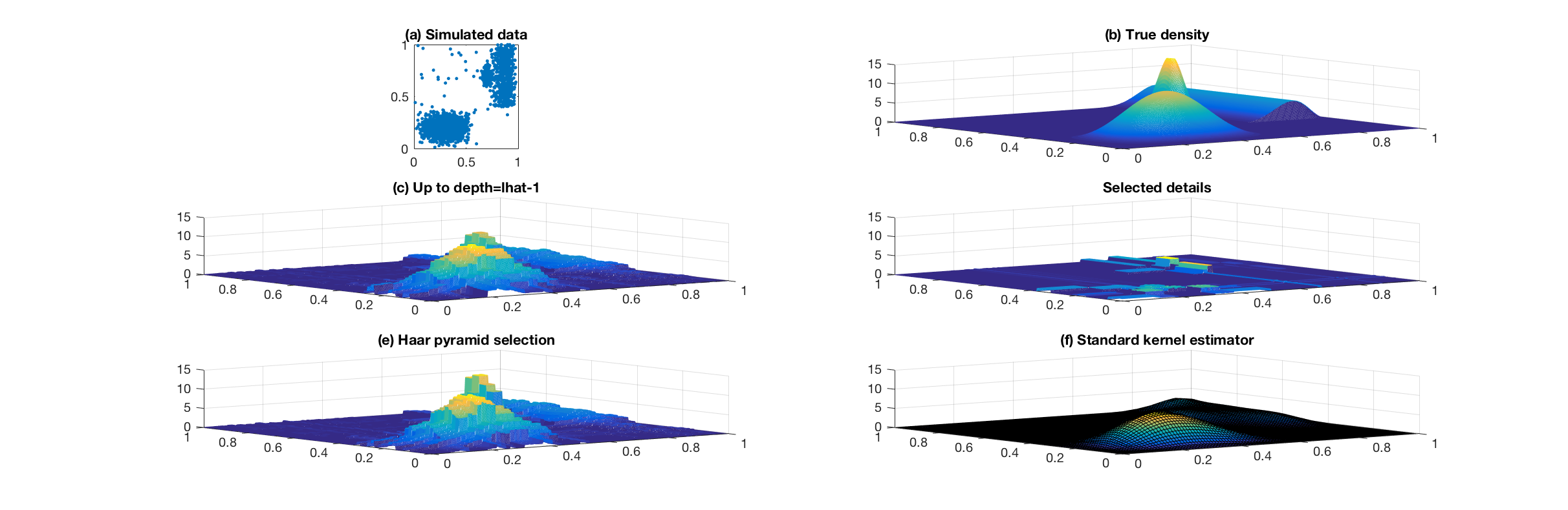
Refer to caption
Figure 1. Pyramid selection and standard kernel for an example of mixture of multiplicative densities.

In the copula density estimation framework, we consider an example where the copula of Xi=(Xi​1,Xi​2)X_{i}=(X_{i1},X_{i2}) is either a Frank copula or a Clayton copula conditionally to a binary variable Z.Z. More precisely, we consider the mixture copula

s⁡(x1,x2)=0.5​sF​(x1,x2)+0.5​sC​(x1,x2)s(x_{1},x_{2})=0.5s_{F}(x_{1},x_{2})+0.5s_{C}(x_{1},x_{2})

where sFs_{F} is the density of a Frank copula with parameter 4 and sCs_{C} is the density of a Clayton copula with parameter 2. These two examples of Archimedean copula densities are shown in Figure 2 and the resulting mixture in Figure 3 (b). We use the same penalty as in the previous example, adapted of course to the copula density estimation framework. We illustrate in Figure 3 the pyramid selection procedure on a sample with size n=2000.n=2000. Though not all theoretical conditions are fully satisfied here, the pyramid selection procedure still provides a reliable estimator.

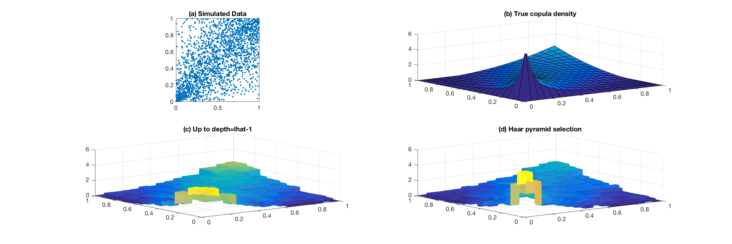
Refer to caption
Figure 2. Left: Frank copula density with parameter 4; Right: Clayton copula density with parameter 2.
Refer to caption
Figure 3. Pyramid selection for an example of mixture copula density.

As a conclusion, those examples suggest that the Haar pyramid selection already provides a useful new estimation procedure. This is most encouraging for pyramid selection based on higher order wavelets, whose full calibration based on an extensive simulation study in each framework will be the subject of another work.

7. Proofs

We shall use repeatedly the classical inequality

(14) 2​a​b≤θ​a2+1θ​b22ab\leq\theta a^{2}+\frac{1}{\theta}b^{2}

for all positive θ,a,b.\theta,a,b.

7.1. Proof of Proposition 2

We only have to prove 2 for m∙.m_{\bullet}. Indeed, as any pyramidal model mm is a subset of m∙,m_{\bullet}, a common upper-bound for the residual terms is

‖sˇm⋆−s^m⋆‖2≤‖sˇm∙⋆−s^m∙⋆‖2.\|\check{s}^{\star}_{m}-\hat{s}^{\star}_{m}\|^{2}\leq\|\check{s}^{\star}_{m_{\bullet}}-\hat{s}^{\star}_{m_{\bullet}}\|^{2}.

Under Assumption (L), and thanks to assumptions S.iii)S.iii) and W.v),W.v), we have that for all 𝝀∈m∙,\bm{\lambda}\in m_{\bullet}, 𝒙=(x1,…,xd)\bm{x}=(x_{1},\ldots,x_{d}) and 𝒚=(y1,…,yd)∈Q,\bm{y}=(y_{1},\ldots,y_{d})\in Q,

|Ψ𝝀​(𝒙)−Ψ𝝀​(𝒚)|≤κd​23​L∙/2​∑k=1d|xk−yk|.|\Psi_{\bm{\lambda}}(\bm{x})-\Psi_{\bm{\lambda}}(\bm{y})|\leq\kappa^{d}2^{3L_{\bullet}/2}\sum_{k=1}^{d}|x_{k}-y_{k}|.

According to Massart’s version of Dworetzky-Kiefer-Wolfowitz inequality (see [32]), for any positive z,z, and 1≤k≤d,1\leq k\leq d, there exists some event Ωk​(z)\Omega_{k}(z) on which ‖F^n​k−Fk‖∞≤z/n\|\hat{F}_{nk}-F_{k}\|_{\infty}\leq z/\sqrt{n} and such that ℙ⁡(Ωkc​(z))≤2​exp⁡(−2​z2).\mathbb{P}(\Omega^{c}_{k}(z))\leq 2\exp(-2z^{2}). Setting Ω(z)=∩k=1dΩk(z),\Omega(z)=\cap_{k=1}^{d}\Omega_{k}(z), we thus have for all 𝝀∈m∙\bm{\lambda}\in m_{\bullet}

|βˇ𝝀−β^𝝀|≤κd​23​L∙/2​d​(z/n)​1​IΩ⁡(z)+κd​23​L∙/2​d​1​IΩc​(z),|\check{\beta}_{\bm{\lambda}}-\widehat{\beta}_{\bm{\lambda}}|\leq\kappa^{d}2^{3L_{\bullet}/2}d(z/\sqrt{n}){1\kern-2.8889pt{}I}_{\Omega(z)}+\kappa^{d}2^{3L_{\bullet}/2}d{1\kern-2.8889pt{}I}_{\Omega^{c}(z)},

hence

𝔼⁡[‖sˇm∙⋆−s^m∙⋆‖2]≤κ2​d​23​L∙​d2​(z2/n+2​d​exp⁡(−2​z2))​Dm∙.\mathbb{E}[\|\check{s}^{\star}_{m_{\bullet}}-\hat{s}^{\star}_{m_{\bullet}}\|^{2}]\leq\kappa^{2d}2^{3L_{\bullet}}d^{2}(z^{2}/n+2d\exp(-2z^{2}))D_{m_{\bullet}}.

Finally, Dm∙D_{m_{\bullet}} is of order L∙d−1​2L∙L^{d-1}_{\bullet}2^{L_{\bullet}} (see Proposition 4), so by choosing 2​z2=log⁡(n),2z^{2}=\log(n),

𝔼⁡[‖sˇm∙⋆−s^m∙⋆‖2]≤C⁡(κ,d)​L∙d−1​24​L∙​log⁡(n)/n.\mathbb{E}[\|\check{s}^{\star}_{m_{\bullet}}-\hat{s}^{\star}_{m_{\bullet}}\|^{2}]\leq C(\kappa,d)L^{d-1}_{\bullet}2^{4L_{\bullet}}\log(n)/n.

7.2. Proof of Proposition 3

For all bounded measurable function g,g, let us denote DΔ​(g)=𝔼⁡[g⁡(XΔ)]/Δ−∫Qg​s.D_{\Delta}(g)=\mathbb{E}[g(X_{\Delta})]/\Delta-\int_{Q}gs. For all 𝝀∈Λ,\bm{\lambda}\in\Lambda,

(15) 𝔼⁡[(βˇ𝝀−β^𝝀)2]≤4​(Var​(βˇ𝝀)+Var​(β^𝝀)+DΔ2​(Ψ𝝀))≤8​‖s‖∞n​Δ+4​DΔ​(Ψ𝝀2)n​Δ+4​DΔ2​(Ψ𝝀).\mathbb{E}\left[\left(\check{\beta}_{\bm{\lambda}}-\widehat{\beta}_{\bm{\lambda}}\right)^{2}\right]\leq 4\left(\text{{Var}}(\check{\beta}_{\bm{\lambda}})+\text{{Var}}(\widehat{\beta}_{\bm{\lambda}})+D^{2}_{\Delta}(\Psi_{\bm{\lambda}})\right)\leq 8\frac{\|s\|_{\infty}}{n\Delta}+4\frac{D_{\Delta}(\Psi^{2}_{\bm{\lambda}})}{n\Delta}+4D^{2}_{\Delta}(\Psi_{\bm{\lambda}}).

We shall bound DΔ​(Ψ𝝀)D_{\Delta}(\Psi_{\bm{\lambda}}) by using the decomposition of a Lévy process into a big jump compound Poisson process and an independent small jump Lévy process. Let us fix ε>0\varepsilon>0 small enough so that Q=∏k=1d[ak,bk]⊂{∥x∥>ε}Q=\prod_{k=1}^{d}[a_{k},b_{k}]\subset\{\|x\|>\varepsilon\} and denote by (Σ,𝝁,ν)(\Sigma,\bm{\mu},\nu) the characteristic Lévy triplet of 𝐗=(Xt)t≥0,\mathbf{X}=(X_{t})_{t\geq 0}, where 𝝁\bm{\mu} stands for the drift and ν\nu is the Lévy measure, with density ff with respect to the Lebesgue measure on ℝd\mathbb{R}^{d} (see Section 2.2). Then 𝐗\mathbf{X} is distributed as 𝐗ε+𝐗~ε,\mathbf{X}^{\varepsilon}+\tilde{\mathbf{X}}^{\varepsilon}, where 𝐗ε\mathbf{X}^{\varepsilon} and 𝐗~ε\tilde{\mathbf{X}}^{\varepsilon} are independent Lévy processes with following characteristics. First, 𝐗ε\mathbf{X}^{\varepsilon} is a Lévy process with characteristic Lévy triplet (Σ,𝝁ε,νϵ),(\Sigma,\bm{\mu}_{\varepsilon},\nu_{\epsilon}), where the drift is

𝝁ε=𝝁−∫ε<‖x‖≤1x​f​(x)​𝑑x.\bm{\mu}_{\varepsilon}=\bm{\mu}-\int_{\varepsilon<\|x\|\leq 1}x\ f(x)\mathrm{d}x.

and the Lévy measure is

νε​(d​x)=1​I‖x‖≤ε​f​(x)​d​x.\nu_{\varepsilon}(\mathrm{d}x)={1\kern-2.8889pt{}I}_{\|x\|\leq\varepsilon}f(x)\mathrm{d}x.

The process 𝐗~ε\tilde{\mathbf{X}}^{\varepsilon} is the compound Poisson process

X~tε=∑i=1N~tξi,\tilde{X}_{t}^{\varepsilon}=\sum_{i=1}^{\tilde{N}_{t}}\xi_{i},

where N~\tilde{N} is a homogeneous Poisson process with intensity λε=ν({∥x∥>ε}),\lambda_{\varepsilon}=\nu(\{\|x\|>\varepsilon\}), (ξi)i≥1(\xi_{i})_{i\geq 1} are i.i.d. with density λε−1​1​I‖x‖>ε​f​(x),\lambda_{\varepsilon}^{-1}{1\kern-2.8889pt{}I}_{\|x\|>\varepsilon}f(x), and N~\tilde{N} and (ξi)i≥1(\xi_{i})_{i\geq 1} are independent.

Conditioning by N~\tilde{N} and using the aforementioned independence properties yields

𝔼⁡[Ψ𝝀​(XΔ)]Δ=e−λε​Δ​𝔼⁡[Ψ𝝀​(XΔε)]Δ+λε​e−λε​Δ​𝔼​[Ψ𝝀​(XΔε+ξ1)]+λε2​Δ​e−λε​Δ​∑j=0∞𝔼⁡[Ψ𝝀​(XΔε+∑i=1j+2ξi)]​(λε​Δ)j(j+2)!.\frac{\mathbb{E}[\Psi_{\bm{\lambda}}(X_{\Delta})]}{\Delta}=e^{-\lambda_{\varepsilon}\Delta}\frac{\mathbb{E}[\Psi_{\bm{\lambda}}(X^{\varepsilon}_{\Delta})]}{\Delta}+\lambda_{\varepsilon}e^{-\lambda_{\varepsilon}\Delta}\mathbb{E}[\Psi_{\bm{\lambda}}(X^{\varepsilon}_{\Delta}+\xi_{1})]+\lambda^{2}_{\varepsilon}\Delta e^{-\lambda_{\varepsilon}\Delta}\sum_{j=0}^{\infty}\mathbb{E}\left[\Psi_{\bm{\lambda}}\left(X^{\varepsilon}_{\Delta}+\sum_{i=1}^{j+2}\xi_{i}\right)\right]\frac{(\lambda_{\varepsilon}\Delta)^{j}}{(j+2)!}.

Conditioning by ξ1\xi_{1} and using independence between XΔεX^{\varepsilon}_{\Delta} and ξ1\xi_{1} then yields

λε​𝔼​[Ψ𝝀​(XΔε+ξ1)]=∫‖x‖>ε𝔼⁡[Ψ𝝀​(XΔε+x)]​f​(x)​𝑑x.\lambda_{\varepsilon}\mathbb{E}[\Psi_{\bm{\lambda}}(X^{\varepsilon}_{\Delta}+\xi_{1})]=\int_{\|x\|>\varepsilon}\mathbb{E}[\Psi_{\bm{\lambda}}(X^{\varepsilon}_{\Delta}+x)]f(x)\mathrm{d}x.

Writing ⟨Ψ𝝀,s⟩=e−λε​Δ​⟨Ψ𝝀,s⟩+(1−e−λε​Δ)​⟨Ψ𝝀,s⟩\langle\Psi_{\bm{\lambda}},s\rangle=e^{-\lambda_{\varepsilon}\Delta}\langle\Psi_{\bm{\lambda}},s\rangle+(1-e^{-\lambda_{\varepsilon}\Delta})\langle\Psi_{\bm{\lambda}},s\rangle and using (1−e−λε​Δ)≤λε​Δ(1-e^{-\lambda_{\varepsilon}\Delta})\leq\lambda_{\varepsilon}\Delta leads to

|DΔ​(Ψ𝝀)|≤RΔ(1)​(Ψ𝝀)+RΔ(2)​(Ψ𝝀)+RΔ(3)​(Ψ𝝀)+RΔ(4)​(Ψ𝝀),|D_{\Delta}(\Psi_{\bm{\lambda}})|\leq R_{\Delta}^{(1)}(\Psi_{\bm{\lambda}})+R_{\Delta}^{(2)}(\Psi_{\bm{\lambda}})+R_{\Delta}^{(3)}(\Psi_{\bm{\lambda}})+R_{\Delta}^{(4)}(\Psi_{\bm{\lambda}}),

where

RΔ(1)​(Ψ𝝀)=e−λε​Δ​𝔼⁡[Ψ𝝀​(XΔε)]Δ,RΔ(2)​(Ψ𝝀)=e−λε​Δ​∫‖x‖>ε|𝔼⁡[Ψ𝝀​(XΔε+x)−Ψ𝝀​(x)]|​f​(x)​𝑑x,R_{\Delta}^{(1)}(\Psi_{\bm{\lambda}})=e^{-\lambda_{\varepsilon}\Delta}\frac{\mathbb{E}[\Psi_{\bm{\lambda}}(X^{\varepsilon}_{\Delta})]}{\Delta},\quad R_{\Delta}^{(2)}(\Psi_{\bm{\lambda}})=e^{-\lambda_{\varepsilon}\Delta}\int_{\|x\|>\varepsilon}\left|\mathbb{E}\left[\Psi_{\bm{\lambda}}(X^{\varepsilon}_{\Delta}+x)-\Psi_{\bm{\lambda}}(x)\right]\right|f(x)\mathrm{d}x,
(16) RΔ(3)​(Ψ𝝀)=λε​Δ​‖Ψ𝝀‖1​‖s‖∞,RΔ(4)​(Ψ𝝀)=λε2​Δ​‖Ψ𝝀‖∞.R_{\Delta}^{(3)}(\Psi_{\bm{\lambda}})=\lambda_{\varepsilon}\Delta\|\Psi_{\bm{\lambda}}\|_{1}\|s\|_{\infty},\quad R_{\Delta}^{(4)}(\Psi_{\bm{\lambda}})=\lambda_{\varepsilon}^{2}\Delta\|\Psi_{\bm{\lambda}}\|_{\infty}.

As Ψ𝝀\Psi_{\bm{\lambda}} has compact support Q,Q,

RΔ(1)​(Ψ𝝀)≤e−λε​Δ​‖Ψ𝝀‖∞​ℙ⁡(XΔε∈Q)Δ.R_{\Delta}^{(1)}(\Psi_{\bm{\lambda}})\leq e^{-\lambda_{\varepsilon}\Delta}\|\Psi_{\bm{\lambda}}\|_{\infty}\frac{\mathbb{P}(X^{\varepsilon}_{\Delta}\in Q)}{\Delta}.

Let us denote by XΔ,kεX^{\varepsilon}_{\Delta,k} the kk-th coordinate of XΔεX^{\varepsilon}_{\Delta} and by dQd_{Q} the maximal distance from [ak,bk][a_{k},b_{k}] to 0, for k=1,…,d,k=1,\ldots,d, reached for instance at k=k0.k=k_{0}. We deduce from the proof of Lemma 2 in [48] (see also [23], equation (3.3)) that there exists z0=z0​(ε)z_{0}=z_{0}(\varepsilon) such that if Δ<dQ/z0​(ε),\Delta<d_{Q}/z_{0}(\varepsilon),

ℙ⁡(XΔε∈Q)≤ℙ⁡(|XΔ,k0ε|≥dQ)≤exp⁡((z0​log⁡(z0)+u−u​log⁡(u))/(2​ε))​ΔdQ/(2​ε)\mathbb{P}(X^{\varepsilon}_{\Delta}\in Q)\leq\mathbb{P}(|X^{\varepsilon}_{\Delta,k_{0}}|\geq d_{Q})\leq\exp\left((z_{0}\log(z_{0})+u-u\log(u))/(2\varepsilon)\right)\Delta^{d_{Q}/(2\varepsilon)}

so that

(17) RΔ(1)​(Ψ𝝀)≤C⁡(dQ,ε)​e−λε​Δ​‖Ψ𝝀‖∞​ΔdQ/(2​ε)−1.R_{\Delta}^{(1)}(\Psi_{\bm{\lambda}})\leq C(d_{Q},\varepsilon)e^{-\lambda_{\varepsilon}\Delta}\|\Psi_{\bm{\lambda}}\|_{\infty}\Delta^{d_{Q}/(2\varepsilon)-1}.

Under Assumption (L),(L), Ψ𝝀\Psi_{\bm{\lambda}} is Lipschitz on Q,Q, so

|Ψ𝝀(XΔε+x)−Ψ𝝀(x)|≤∥Ψ𝝀∥L∥XΔε∥11I{XΔε+x∈Q}∩{x∈Q}+|Ψ𝝀(x)|1I{XΔε+x∉Q}∩{x∈Q}+∥Ψ𝝀∥∞1I{XΔε+x∈Q}∩{x∉Q}.\left|\Psi_{\bm{\lambda}}(X^{\varepsilon}_{\Delta}+x)-\Psi_{\bm{\lambda}}(x)\right|\leq\|\Psi_{\bm{\lambda}}\|_{L}\|X_{\Delta}^{\varepsilon}\|_{1}{1\kern-2.8889pt{}I}_{\{X_{\Delta}^{\varepsilon}+x\in Q\}\cap\{x\in Q\}}+|\Psi_{\bm{\lambda}}(x)|{1\kern-2.8889pt{}I}_{\{X_{\Delta}^{\varepsilon}+x\notin Q\}\cap\{x\in Q\}}+\|\Psi_{\bm{\lambda}}\|_{\infty}{1\kern-2.8889pt{}I}_{\{X_{\Delta}^{\varepsilon}+x\in Q\}\cap\{x\notin Q\}}.

Besides, as QQ is compact and bounded away from the origin, there exists δQ\delta_{Q} and ρQ>0\rho_{Q}>0 such that

{XΔε+x∈Q}∩{x∈Q}⊂{∥XΔε∥≥δQ}\{X_{\Delta}^{\varepsilon}+x\in Q\}\cap\{x\in Q\}\subset\{\|X_{\Delta}^{\varepsilon}\|\geq\delta_{Q}\}
({XΔε+x∈Q}∩{x∉Q})∪({XΔε+x∉Q}∩{x∈Q})⊂{∥XΔε∥≥ρQ}(\{X_{\Delta}^{\varepsilon}+x\in Q\}\cap\{x\notin Q\})\cup(\{X_{\Delta}^{\varepsilon}+x\notin Q\}\cap\{x\in Q\})\subset\{\|X_{\Delta}^{\varepsilon}\|\geq\rho_{Q}\}

The Lévy measure of 𝐗ε\mathbf{X}^{\varepsilon} is compactly supported and satisfies

∫‖x‖2​νε​(𝑑x)=∫‖x‖≤ε‖x‖2​ν​(𝑑x)\int\|x\|^{2}\nu_{\varepsilon}(\mathrm{d}x)=\int_{\|x\|\leq\varepsilon}\|x\|^{2}\nu(\mathrm{d}x)

which is finite since ν\nu is a Lévy measure (see for instance [49], Theorem 8.1). So we deduce from [34], Theorem 2.1, that

𝔼⁡[‖XΔε‖2]≤C⁡(d,f)​Δ,\mathbb{E}\left[\|X_{\Delta}^{\varepsilon}\|^{2}\right]\leq C(d,f)\Delta,

hence

𝔼⁡[‖XΔε‖1​1​I‖XΔε‖≥δQ]≤C⁡(d)​δQ−1​𝔼​[‖XΔε‖2]≤C⁡(d,f)​δQ−1​Δ\mathbb{E}\left[\|X_{\Delta}^{\varepsilon}\|_{1}{1\kern-2.8889pt{}I}_{\|X_{\Delta}^{\varepsilon}\|\geq\delta_{Q}}\right]\leq C(d)\delta_{Q}^{-1}\mathbb{E}\left[\|X_{\Delta}^{\varepsilon}\|^{2}\right]\leq C(d,f)\delta_{Q}^{-1}\Delta

and from Markov inequality

ℙ⁡(‖XΔε‖≥ρQ)≤C⁡(d,f)​ρQ−2​Δ.\mathbb{P}(\|X^{\varepsilon}_{\Delta}\|\geq\rho_{Q})\leq C(d,f)\rho_{Q}^{-2}\Delta.

Finally, fixing 0<ε<min⁡(dQ/4,infx∈Q‖x‖),0<\varepsilon<\min(d_{Q}/4,\inf_{x\in Q}\|x\|), we have for all 0<Δ<min⁡(dQ/z0​(ϵ),1)0<\Delta<\min(d_{Q}/z_{0}(\epsilon),1)

(18) RΔ(2)​(Ψ𝝀)≤C⁡(d,f)​e−λε​Δ​Δ​(δQ−1​λε​‖Ψ𝝀‖L+ρQ−2​‖s‖∞​‖Ψ𝝀‖1+ρQ−2​λε​‖Ψ𝝀‖∞).R_{\Delta}^{(2)}(\Psi_{\bm{\lambda}})\leq C(d,f)e^{-\lambda_{\varepsilon}\Delta}\Delta(\delta_{Q}^{-1}\lambda_{\varepsilon}\|\Psi_{\bm{\lambda}}\|_{L}+\rho_{Q}^{-2}\|s\|_{\infty}\|\Psi_{\bm{\lambda}}\|_{1}+\rho_{Q}^{-2}\lambda_{\varepsilon}\|\Psi_{\bm{\lambda}}\|_{\infty}).

For all 𝝀∈m∙,\bm{\lambda}\in m_{\bullet},

max⁡(‖Ψ𝝀‖L,‖Ψ𝝀‖∞,‖Ψ𝝀‖1)≤C⁡(κ)​23​L∙/2,max⁡(‖Ψ𝝀2‖L,‖Ψ𝝀2‖∞,‖Ψ𝝀2‖1)≤C⁡(κ)​22​L∙,\max(\|\Psi_{\bm{\lambda}}\|_{L},\|\Psi_{\bm{\lambda}}\|_{\infty},\|\Psi_{\bm{\lambda}}\|_{1})\leq C(\kappa)2^{3L_{\bullet}/2},\max(\|\Psi^{2}_{\bm{\lambda}}\|_{L},\|\Psi^{2}_{\bm{\lambda}}\|_{\infty},\|\Psi^{2}_{\bm{\lambda}}\|_{1})\leq C(\kappa)2^{2L_{\bullet}},

so that combining (15), (17), (18) and (16) yields

𝔼⁡[‖sˇm⋆−s^m⋆‖2]≤8​‖s‖∞​Dmn​Δ+C⁡(κ,d,f,Q,ε)​L∙d−1​24​L∙​n​Δ3+23​L∙​Δn​Δ.\mathbb{E}[\|\check{s}^{\star}_{m}-\hat{s}^{\star}_{m}\|^{2}]\leq 8\frac{\|s\|_{\infty}D_{m}}{n\Delta}+C(\kappa,d,f,Q,\varepsilon)L_{\bullet}^{d-1}\frac{2^{4L_{\bullet}}n\Delta^{3}+2^{3L_{\bullet}}\Delta}{n\Delta}.

7.3. Proof of Proposition 4

Due to hypotheses S.ii)S.ii) and W.ii),W.ii), we have for all j≥j0,j\geq j_{0},

2j−1≤♯​∇j≤M​2j−1,2^{j-1}\leq\sharp\nabla_{j}\leq M2^{j-1},

hence, for all 𝒋∈ℕj0d,\bm{j}\in\mathbb{N}_{j_{0}}^{d},

(1/2)d​2|𝒋|≤♯​∇𝒋≤(M/2)d​2|𝒋|.(1/2)^{d}2^{|\bm{j}|}\leq\sharp\bm{\nabla}_{\bm{j}}\leq(M/2)^{d}2^{|\bm{j}|}.

Let us fix ℓ∈{d​j0,…,L∙}.\ell\in\{dj_{0},\ldots,L_{\bullet}\}. The number of dd-uples 𝒋∈ℕj0d\bm{j}\in\mathbb{N}_{j_{0}}^{d} such that |𝒋|=ℓ|\bm{j}|=\ell is equal to the number of partititions of the integer ℓ−d​j0\ell-dj_{0} into dd nonnegative integers, hence

♯​𝑱ℓ=(ℓ−d​j0+d−1d−1)=∏k=1d−1(1+ℓ−d​j0k).\sharp\bm{J}_{\ell}=\binom{\ell-dj_{0}+d-1}{d-1}=\prod_{k=1}^{d-1}\left(1+\frac{\ell-dj_{0}}{k}\right).

The last two displays and the classical upper-bound for binomial coefficient (see for instance [33], Proposition 2.5) yield

(19) c0(d)(ℓ−dj0+d−1)d−12ℓ≤♯U∇(ℓ)≤c1(M,d)(ℓ−dj0+d−1)d−12ℓ,c_{0}(d)(\ell-dj_{0}+d-1)^{d-1}2^{\ell}\leq\sharp U\bm{\nabla}(\ell)\leq c_{1}(M,d)(\ell-dj_{0}+d-1)^{d-1}2^{\ell},

where c0​(d)=2−d​(d−1)−(d−1)c_{0}(d)=2^{-d}(d-1)^{-(d-1)} and c1​(M,d)=(M/2)d​(e/(d−1))d−1.c_{1}(M,d)=(M/2)^{d}(e/(d-1))^{d-1}.

Let us now fix ℓ1∈{d​j0+1,…,L∙+1}.\ell_{1}\in\{dj_{0}+1,\ldots,L_{\bullet}+1\}. Any model m∈ℳℓ1𝒫m\in\mathcal{M}^{\mathcal{P}}_{\ell_{1}} satisfies

Dm=∑ℓ=d​j0ℓ1−1♯U∇(ℓ)+∑k=0L∙−ℓ1N(ℓ1,k).D_{m}=\sum_{\ell=dj_{0}}^{\ell_{1}-1}\sharp U\bm{\nabla}(\ell)+\sum_{k=0}^{L_{\bullet}-\ell_{1}}N(\ell_{1},k).

So we obviously have

Dm≥♯U∇(ℓ1−1)≥κ1(d)(ℓ1−dj0+d−2)d−12ℓ1,D_{m}\geq\sharp U\bm{\nabla}(\ell_{1}-1)\geq\kappa_{1}(d)(\ell_{1}-dj_{0}+d-2)^{d-1}2^{\ell_{1}},

with κ1​(d)=c0​(d)/2=2−(d+1)​(d−1)−(d−1).\kappa_{1}(d)=c_{0}(d)/2=2^{-(d+1)}(d-1)^{-(d-1)}. Besides, with our choice of N⁡(ℓ1,k),N(\ell_{1},k),

Dm≤c1​(M,d)​(ℓ1−d​j0+d−2)d−1​∑ℓ=d​j0ℓ1−12ℓ+2​M−d​c1​(M,d)​s1​(d)​(ℓ1−d​j0+d−2)d−1​2ℓ1,D_{m}\leq c_{1}(M,d)(\ell_{1}-dj_{0}+d-2)^{d-1}\sum_{\ell=dj_{0}}^{\ell_{1}-1}2^{\ell}+2M^{-d}c_{1}(M,d)s_{1}(d)(\ell_{1}-dj_{0}+d-2)^{d-1}2^{\ell_{1}},

so that Proposition 4 holds with κ2​(d,j0,B)=c1​(M,d)​(1+2​M−d​c1​(M,d)​s1​(d)),\kappa_{2}(d,j_{0},B)=c_{1}(M,d)(1+2M^{-d}c_{1}(M,d)s_{1}(d)), where

s1​(d)=∑k=0∞(1+k/(d−1))d−1(2+k)d+2.s_{1}(d)=\sum_{k=0}^{\infty}\frac{(1+k/(d-1))^{d-1}}{(2+k)^{d+2}}.

The number of subsets of Λ\Lambda in ℳℓ1𝒫\mathcal{M}^{\mathcal{P}}_{\ell_{1}} satisfies

♯​ℳℓ1𝒫=∏k=0L∙−ℓ1(♯U∇(ℓ1+k)N⁡(ℓ1,k))≤∏k=0L∙−ℓ1(e♯U∇(ℓ1+k)N⁡(ℓ1,k))N⁡(ℓ1,k).\sharp\mathcal{M}^{\mathcal{P}}_{\ell_{1}}=\prod_{k=0}^{L_{\bullet}-\ell_{1}}\binom{\sharp U\bm{\nabla}(\ell_{1}+k)}{N(\ell_{1},k)}\leq\prod_{k=0}^{L_{\bullet}-\ell_{1}}\left(\frac{e\>\sharp U\bm{\nabla}(\ell_{1}+k)}{N(\ell_{1},k)}\right)^{N(\ell_{1},k)}.

For k∈{0,…,L∙−ℓ1},k\in\{0,\ldots,L_{\bullet}-\ell_{1}\}, let f⁡(k)=(k+2)d+2​2k​Md/2,f(k)=(k+2)^{d+2}2^{k}M^{d}/2, then N(ℓ1,k)≤♯U∇(ℓ1+k)/f(k).N(\ell_{1},k)\leq\sharp U\bm{\nabla}(\ell_{1}+k)/f(k). As the function x∈[0,U]↦x​log⁡(e​U/x)x\in[0,U]\mapsto x\log(eU/x) is increasing, we deduce

log⁡(♯​ℳℓ1𝒫)≤D⁡(ℓ1)​∑k=0L∙−ℓ1♯U∇(ℓ1+k)♯U∇(ℓ1−1)​1+log⁡(f⁡(k))f⁡(k).\log(\sharp\mathcal{M}^{\mathcal{P}}_{\ell_{1}})\leq D(\ell_{1})\sum_{k=0}^{L_{\bullet}-\ell_{1}}\frac{\sharp U\bm{\nabla}(\ell_{1}+k)}{\sharp U\bm{\nabla}(\ell_{1}-1)}\frac{1+\log(f(k))}{f(k)}.

Setting

s2=∑k=0∞1(k+2)3,s3=∑k=0∞log⁡(k+2)(k+2)3,s4=∑k=0∞1(k+2)2,s_{2}=\sum_{k=0}^{\infty}\frac{1}{(k+2)^{3}},\quad s_{3}=\sum_{k=0}^{\infty}\frac{\log(k+2)}{(k+2)^{3}},s_{4}=\sum_{k=0}^{\infty}\frac{1}{(k+2)^{2}},

one may take for instance κ3​(j0,B,d)=(log⁡(e/2)+d​log⁡(M))​s2+(d+2)​s3+log⁡(2)​s4\kappa_{3}(j_{0},B,d)=(\log(e/2)+d\log(M))s_{2}+(d+2)s_{3}+\log(2)s_{4} in Proposition 4.

7.4. Proof of Theorem 1

7.4.1. Notation and preliminary results

Hyperbolic wavelet bases inherit from the underlying univariate wavelet bases a localization property which can be stated as follows.

Lemma 1.

Let D¯​(L∙)=(e⁡(L∙−d​j0+d−1)/(d−1))d−1​2L∙/2,\underline{D}(L_{\bullet})=\left(e(L_{\bullet}-dj_{0}+d-1)/(d-1)\right)^{d-1}2^{L_{\bullet}/2}, then for all real-valued sequence (a𝛌)𝛌∈m∙,(a_{\bm{\lambda}})_{\bm{\lambda}\in m_{\bullet}},

max⁡{‖∑𝝀∈m∙a𝝀​Ψ𝝀‖∞,‖∑𝝀∈m∙a𝝀​Ψ𝝀⋆‖∞}≤κ7′​max𝝀∈m∙​|a𝝀|​D¯​(L∙),\max\left\{\left\|\sum_{\bm{\lambda}\in m_{\bullet}}a_{\bm{\lambda}}\Psi_{\bm{\lambda}}\right\|_{\infty},\left\|\sum_{\bm{\lambda}\in m_{\bullet}}a_{\bm{\lambda}}\Psi^{\star}_{\bm{\lambda}}\right\|_{\infty}\right\}\leq\kappa^{\prime}_{7}\max_{{\bm{\lambda}}\in m_{\bullet}}|a_{\bm{\lambda}}|\underline{D}(L_{\bullet}),

where κ7′=κ2​d​(2+2)\kappa^{\prime}_{7}=\kappa^{2d}(2+\sqrt{2}) for instance.

Proof.

For all 𝐱=(x1,…,xd)∈[0,1]d,\mathbf{x}=(x_{1},\ldots,x_{d})\in[0,1]^{d}, using assumptions S.vi),S.vii),S.viii),W.iv),W.v),W.vi)S.vi),S.vii),S.viii),W.iv),W.v),W.vi) in Section 3.1, we get

|∑𝝀∈m∙a𝝀​Ψ𝝀|\displaystyle\left|\sum_{\bm{\lambda}\in m_{\bullet}}a_{\bm{\lambda}}\Psi_{\bm{\lambda}}\right| ≤max𝝀∈m∙⁡|a𝝀|​∑ℓ=d​j0L∙∑𝒋∈𝑱ℓ∏k=1d(∑λk∈∇jk|ψλk​(xk)|)\displaystyle\leq\max_{\bm{\lambda}\in m_{\bullet}}\left|a_{\bm{\lambda}}\right|\sum_{\ell=dj_{0}}^{L_{\bullet}}\sum_{\bm{j}\in\bm{J}_{\ell}}\prod_{k=1}^{d}\left(\sum_{\lambda_{k}\in\nabla_{j_{k}}}|\psi_{\lambda_{k}}(x_{k})|\right)
≤κ2​d​max𝝀∈m∙​|a𝝀|​∑ℓ=d​j0L∙∑𝒋∈𝑱ℓ2ℓ/2.\displaystyle\leq\kappa^{2d}\max_{\bm{\lambda}\in m_{\bullet}}\left|a_{\bm{\lambda}}\right|\sum_{\ell=dj_{0}}^{L_{\bullet}}\sum_{\bm{j}\in\bm{J}_{\ell}}2^{\ell/2}.

We deduce from the proof of Proposition 4 the upper-bound ♯​𝑱ℓ≤(e⁡(L∙−d​j0+d−1)/(d−1))d−1\sharp\bm{J}_{\ell}\leq\left(e(L_{\bullet}-dj_{0}+d-1)/(d-1)\right)^{d-1} which allows to conclude. ∎

For all t∈𝕃2​([0,1]d),t\in\mathbb{L}_{2}([0,1]^{d}), we define

ν⁡(t)=∑𝝀∈Λ⟨t,Ψ𝝀⟩​(βˇ𝝀−⟨s,Ψ𝝀⟩),νR​(t)=∑𝝀∈Λ⟨t,Ψ𝝀⟩​(β^𝝀−βˇ𝝀),ν^​(t)=ν⁡(t)+νR​(t),\nu(t)=\sum_{\bm{\lambda}\in\Lambda}\langle t,\Psi_{\bm{\lambda}}\rangle(\check{\beta}_{\bm{\lambda}}-\langle s,\Psi_{\bm{\lambda}}\rangle),\quad\nu_{R}(t)=\sum_{\bm{\lambda}\in\Lambda}\langle t,\Psi_{\bm{\lambda}}\rangle(\hat{\beta}_{\bm{\lambda}}-\check{\beta}_{\bm{\lambda}}),\quad\hat{\nu}(t)=\nu(t)+\nu_{R}(t),

and for all m∈ℳ𝒫,m\in\mathcal{M}^{\mathcal{P}}, we set

χ⁡(m)=supt∈Sm⋆|‖t‖𝚿=1ν⁡(t),χR​(m)=supt∈Sm⋆|‖t‖𝚿=1νR​(t).\chi(m)=\sup_{t\in S^{\star}_{m}|\|t\|_{\bm{\Psi}}=1}\nu(t),\quad\chi_{R}(m)=\sup_{t\in S^{\star}_{m}|\|t\|_{\bm{\Psi}}=1}\nu_{R}(t).
Lemma 2.

For all m∈ℳ𝒫,m\in\mathcal{M}^{\mathcal{P}}, let tm⋆=∑𝛌∈m(ν⁡(Ψ𝛌⋆)/χ⁡(m))​Ψ𝛌⋆,t^{\star}_{m}=\sum_{\bm{\lambda}\in m}(\nu(\Psi^{\star}_{\bm{\lambda}})/\chi(m))\Psi^{\star}_{\bm{\lambda}}, then

χ⁡(m)=∑𝝀∈mν2​(Ψ𝝀⋆)=‖sm⋆−sˇm⋆‖𝚿=ν⁡(tm⋆),\chi(m)=\sqrt{\sum_{\bm{\lambda}\in m}\nu^{2}(\Psi^{\star}_{\bm{\lambda}})}=\|s^{\star}_{m}-\check{s}^{\star}_{m}\|_{\bm{\Psi}}=\nu(t^{\star}_{m}),
χR​(m)=∑𝝀∈mνR2​(Ψ𝝀⋆)=‖sˇm⋆−s^m⋆‖𝚿.\chi_{R}(m)=\sqrt{\sum_{\bm{\lambda}\in m}\nu_{R}^{2}(\Psi^{\star}_{\bm{\lambda}})}=\|\check{s}^{\star}_{m}-\hat{s}^{\star}_{m}\|_{\bm{\Psi}}.
Proof.

The proof follows from the linearity of ν\nu and νR\nu_{R} and Cauchy-Schwarz inequality. ∎

Lemma 3.

Let ϵ=κ2′​‖s‖∞/(κ3′​κ7′​D¯​(L∙))\epsilon=\kappa^{\prime}_{2}\|s\|_{\infty}/(\kappa^{\prime}_{3}\kappa^{\prime}_{7}\underline{D}(L_{\bullet})) and

ΩT=∩𝝀∈m∙{|ν(Ψ𝝀⋆)|≤ϵ}.\Omega_{T}=\cap_{\bm{\lambda}\in m_{\bullet}}\left\{|\nu(\Psi^{\star}_{\bm{\lambda}})|\leq\epsilon\right\}.

For all x>0,x>0, there exists a measurable event Ωm​(x)\Omega_{m}(x) on which

χ2​(m)​1​IΩT∩Ωσ≤2​κ1′2​κ5′​∑𝝀∈mmax⁡{σ^𝝀2,1}n¯+8​κ2′​‖s‖∞​xn¯.\chi^{2}(m){1\kern-3.08443pt{}I}_{\Omega_{T}\cap\Omega_{\sigma}}\leq 2\kappa^{\prime 2}_{1}\kappa^{\prime}_{5}\sum_{\bm{\lambda}\in m}\frac{\max\{\hat{\sigma}^{2}_{\bm{\lambda}},1\}}{\bar{n}}+8\kappa^{\prime}_{2}\|s\|_{\infty}\frac{x}{\bar{n}}.

and such that ℙ⁡(Ωmc​(x))≤exp⁡(−x).\mathbb{P}(\Omega^{c}_{m}(x))\leq\exp(-x).

Proof.

We observe that χ⁡(m)=𝒵⁡(𝒯m)\chi(m)=\mathcal{Z}(\mathcal{T}_{m}) where 𝒯m={t∈Sm⋆|‖t‖𝚿=1}.\mathcal{T}_{m}=\{t\in S^{\star}_{m}|\|t\|_{\bm{\Psi}}=1\}. Let us set z=κ2′​‖s‖∞​x/n¯z=\sqrt{\kappa^{\prime}_{2}\|s\|_{\infty}x/\bar{n}} and consider a countable and dense subset 𝒯m′\mathcal{T}^{\prime}_{m} of {t∈Sm⋆|∥t∥𝚿=1,max𝝀∈m|⟨t,Ψ𝝀⟩|≤ϵ/z}.\{t\in S^{\star}_{m}|\|t\|_{\bm{\Psi}}=1,\max_{\bm{\lambda}\in m}|\langle t,\Psi_{\bm{\lambda}}\rangle|\leq\epsilon/z\}. Thanks to the localization property in Lemma 1,

supt∈𝒯m′‖∑λ∈m∙⟨t,Ψ𝝀⟩​Ψ𝝀‖∞≤κ3′​κ2′​‖s‖∞x/n¯.\sup_{t\in\mathcal{T}^{\prime}_{m}}\left\|\sum_{\lambda\in m_{\bullet}}\langle t,\Psi_{\bm{\lambda}}\rangle\Psi_{\bm{\lambda}}\right\|_{\infty}\leq\kappa^{\prime}_{3}\frac{\sqrt{\kappa^{\prime}_{2}\|s\|_{\infty}}}{\sqrt{x/\bar{n}}}.

So Assumption (Conc) ensures that there exists Ωm​(x)\Omega_{m}(x) such that ℙ⁡(Ωmc​(x))≤exp⁡(−x)\mathbb{P}(\Omega^{c}_{m}(x))\leq\exp(-x) and on which

𝒵⁡(𝒯m′)≤κ1′​𝔼​[𝒵⁡(𝒯m′)]+2​κ2′​‖s‖∞​xn¯,\mathcal{Z}(\mathcal{T}^{\prime}_{m})\leq\kappa^{\prime}_{1}\mathbb{E}\left[\mathcal{Z}(\mathcal{T}^{\prime}_{m})\right]+2\sqrt{\kappa^{\prime}_{2}\|s\|_{\infty}\frac{x}{\bar{n}}},

hence

𝒵2​(𝒯m′)≤2​κ1′2​𝔼2​[𝒵⁡(𝒯m′)]+8​κ2′​‖s‖∞​xn¯.\mathcal{Z}^{2}(\mathcal{T}^{\prime}_{m})\leq 2\kappa^{\prime 2}_{1}\mathbb{E}^{2}\left[\mathcal{Z}(\mathcal{T}^{\prime}_{m})\right]+8\kappa^{\prime}_{2}\|s\|_{\infty}\frac{x}{\bar{n}}.

As Z⁡(𝒯m′)≤χ⁡(m),Z(\mathcal{T}^{\prime}_{m})\leq\chi(m), we obtain by convexity and Lemma 2

𝔼2​[𝒵⁡(𝒯m′)]≤𝔼⁡[χ2​(m)]=∑𝝀∈mVar​(βˇ𝝀).\mathbb{E}^{2}\left[\mathcal{Z}(\mathcal{T}^{\prime}_{m})\right]\leq\mathbb{E}\left[\chi^{2}(m)\right]=\sum_{\bm{\lambda}\in m}\text{{Var}}(\check{\beta}_{\bm{\lambda}}).

On ΩT∩{χ(m)≥z},\Omega_{T}\cap\{\chi(m)\geq z\}, tm⋆t^{\star}_{m} given by Lemma 2 satisfies sup𝝀∈m|⟨tm⋆,Ψ𝝀⟩|≤ϵ/z,\sup_{\bm{\lambda}\in m}|\langle t^{\star}_{m},\Psi_{\bm{\lambda}}\rangle|\leq\epsilon/z, so that χ2​(m)=𝒵2​(𝒯m′),\chi^{2}(m)=\mathcal{Z}^{2}(\mathcal{T}^{\prime}_{m}), while on ΩT∩{χ(m)<z},\Omega_{T}\cap\{\chi(m)<z\}, χ2​(m)<κ2′​‖s‖∞​x/n¯.\chi^{2}(m)<\kappa^{\prime}_{2}\|s\|_{\infty}x/\bar{n}. The proof then follows from Assumption (Var). ∎

7.4.2. Proof of Theorem 1

Let us fix m∈ℳ𝒫.m\in\mathcal{M}^{\mathcal{P}}. From the definition of m^𝒫\hat{m}^{\mathcal{P}} and of s^m⋆,\hat{s}^{\star}_{m}, we get

γ^​(s~𝒫)+pen​(m^𝒫)≤γ^​(sm⋆)+pen​(m).\hat{\gamma}(\tilde{s}^{\mathcal{P}})+\text{{pen}}(\hat{m}^{\mathcal{P}})\leq\hat{\gamma}(s^{\star}_{m})+\text{{pen}}(m).

For all t,u∈𝕃2​([0,1]d),t,u\in\mathbb{L}_{2}([0,1]^{d}),

γ^​(t)−γ^​(u)=‖t−s‖𝚿2−‖u−s‖𝚿2−2​ν^​(t−u),\hat{\gamma}(t)-\hat{\gamma}(u)=\|t-s\|^{2}_{\bm{\Psi}}-\|u-s\|^{2}_{\bm{\Psi}}-2\hat{\nu}(t-u),

so

‖s−s~𝒫‖𝚿2≤‖s−sm⋆‖𝚿2+2​ν^​(s~𝒫−sm⋆)+pen​(m)−pen​(m^𝒫).\|s-\tilde{s}^{\mathcal{P}}\|^{2}_{\bm{\Psi}}\leq\|s-s^{\star}_{m}\|^{2}_{\bm{\Psi}}+2\hat{\nu}(\tilde{s}^{\mathcal{P}}-s^{\star}_{m})+\text{{pen}}(m)-\text{{pen}}(\hat{m}^{\mathcal{P}}).

Using the triangle inequality and Inequality (14) with θ=1/4\theta=1/4 and θ=1,\theta=1, we get

2​ν^​(s~𝒫−sm⋆)\displaystyle 2\hat{\nu}(\tilde{s}^{\mathcal{P}}-s^{\star}_{m}) ≤2​‖s~𝒫−sm⋆‖𝚿​(χ⁡(m∪m^𝒫)+χR​(m∪m^𝒫))\displaystyle\leq 2\|\tilde{s}^{\mathcal{P}}-s^{\star}_{m}\|_{\bm{\Psi}}(\chi(m\cup\hat{m}^{\mathcal{P}})+\chi_{R}(m\cup\hat{m}^{\mathcal{P}}))
≤12​‖s−s~𝒫‖𝚿2+12​‖s−sm⋆‖𝚿2+8​χ2​(m∪m^𝒫)+8​χR2​(m∪m^𝒫),\displaystyle\leq\frac{1}{2}\|s-\tilde{s}^{\mathcal{P}}\|^{2}_{\bm{\Psi}}+\frac{1}{2}\|s-s^{\star}_{m}\|^{2}_{\bm{\Psi}}+8\chi^{2}(m\cup\hat{m}^{\mathcal{P}})+8\chi^{2}_{R}(m\cup\hat{m}^{\mathcal{P}}),

hence

(20) ‖s−s~𝒫‖𝚿2≤3​‖s−sm⋆‖𝚿2+16​χ2​(m∪m^𝒫)+2​(pen​(m)−pen​(m^𝒫))+16​χR2​(m∪m^𝒫).\|s-\tilde{s}^{\mathcal{P}}\|^{2}_{\bm{\Psi}}\leq 3\|s-s^{\star}_{m}\|^{2}_{\bm{\Psi}}+16\chi^{2}(m\cup\hat{m}^{\mathcal{P}})+2(\text{{pen}}(m)-\text{{pen}}(\hat{m}^{\mathcal{P}}))+16\chi^{2}_{R}(m\cup\hat{m}^{\mathcal{P}}).

Let us fix ζ>0\zeta>0 and set ω=κ3​(j0,B,d)+log⁡(2)\omega=\kappa_{3}(j_{0},B,d)+\log(2) and Ω⋆(ζ)=∩m′∈ℳ𝒫Ωm∪m′(ζ+ωDm).\Omega_{\star}(\zeta)=\cap_{m^{\prime}\in\mathcal{M}^{\mathcal{P}}}\Omega_{m\cup m^{\prime}}(\zeta+\omega D_{m}). We deduce from Lemma 3 that on Ω⋆​(ζ)\Omega_{\star}(\zeta)

(21) χ2​(m∪m^𝒫)​1​IΩT∩Ωσ≤2​κ1′2​κ5′​∑𝝀∈m∪m^𝒫max⁡{σ^𝝀2,1}n¯+8​κ2′​‖s‖∞​ω⁡(Dm+Dm^𝒫)n¯+8​κ2′​‖s‖∞​ζn¯.\chi^{2}(m\cup\hat{m}^{\mathcal{P}}){1\kern-2.8889pt{}I}_{\Omega_{T}\cap\Omega_{\sigma}}\leq 2\kappa^{\prime 2}_{1}\kappa^{\prime}_{5}\sum_{\bm{\lambda}\in m\cup\hat{m}^{\mathcal{P}}}\frac{\max\{\hat{\sigma}^{2}_{\bm{\lambda}},1\}}{\bar{n}}+8\kappa^{\prime}_{2}\|s\|_{\infty}\frac{\omega(D_{m}+D_{\hat{m}^{\mathcal{P}}})}{\bar{n}}+8\kappa^{\prime}_{2}\|s\|_{\infty}\frac{\zeta}{\bar{n}}.

Besides, given Proposition 4, our choice of ω\omega leads to

ℙ⁡(Ω⋆c​(ζ))≤e−ζ​∑ℓ=d​j0+1L∙+1exp⁡(−D⁡(ℓ)​(ω−log⁡(♯​ℳℓ𝒫)D⁡(ℓ)))≤e−ζ.\mathbb{P}(\Omega^{c}_{\star}(\zeta))\leq e^{-\zeta}\sum_{\ell=dj_{0}+1}^{L_{\bullet}+1}\exp\left(-D(\ell)\left(\omega-\frac{\log(\sharp\mathcal{M}_{\ell}^{\mathcal{P}})}{D(\ell)}\right)\right)\leq e^{-\zeta}.

Choosing for instance

pen​(m)=c1​∑𝝀∈mσ^𝝀2n¯+c2​R¯​Dmn¯,\text{{pen}}(m)=c_{1}\sum_{\bm{\lambda}\in m}\frac{\hat{\sigma}^{2}_{\bm{\lambda}}}{\bar{n}}+c_{2}\frac{\bar{R}D_{m}}{\bar{n}},

with c1≥16​κ1′2​κ5′c_{1}\geq 16\kappa^{\prime 2}_{1}\kappa^{\prime}_{5} and c2≥64​κ2′​ω+8​κ6′c_{2}\geq 64\kappa^{\prime}_{2}\omega+8\kappa^{\prime}_{6} and integrating with respect to ζ>0,\zeta>0, we deduce from (20), (21), Assumption (Var) and Assumption (Conc) that

(22) 𝔼⁡[‖s−s~𝒫‖𝚿2​1​IΩT∩Ωσ]≤3​‖s−sm⋆‖𝚿2+C​R¯​Dmn¯+64​κ2′​‖s‖∞n¯+8​w⁡(n¯)n¯,\mathbb{E}\left[\|s-\tilde{s}^{\mathcal{P}}\|^{2}_{\bm{\Psi}}{1\kern-2.8889pt{}I}_{\Omega_{T}\cap\Omega_{\sigma}}\right]\leq 3\|s-s^{\star}_{m}\|^{2}_{\bm{\Psi}}+C\frac{\bar{R}D_{m}}{\bar{n}}+64\kappa^{\prime}_{2}\frac{\|s\|_{\infty}}{\bar{n}}+8\frac{w(\bar{n})}{\bar{n}},

where CC may depend on κ1′,κ2′,κ4′,κ5′,κ6′,c1,c2.\kappa^{\prime}_{1},\kappa^{\prime}_{2},\kappa^{\prime}_{4},\kappa^{\prime}_{5},\kappa^{\prime}_{6},c_{1},c_{2}.

In order to bound 𝔼⁡[‖s−s~𝒫‖𝚿2​1​IΩTc∪Ωσc],\mathbb{E}\left[\|s-\tilde{s}^{\mathcal{P}}\|^{2}_{\bm{\Psi}}{1\kern-2.8889pt{}I}_{\Omega^{c}_{T}\cup\Omega^{c}_{\sigma}}\right], we first notice that from the triangle inequality and Lemma 2

‖s−s~𝒫‖𝚿\displaystyle\|s-\tilde{s}^{\mathcal{P}}\|_{\bm{\Psi}} ≤‖s−sm^𝒫⋆‖𝚿+‖sm^𝒫⋆−s^m^𝒫⋆‖𝚿\displaystyle\leq\|s-s^{\star}_{\hat{m}^{\mathcal{P}}}\|_{\bm{\Psi}}+\|s^{\star}_{\hat{m}^{\mathcal{P}}}-\hat{s}^{\star}_{\hat{m}^{\mathcal{P}}}\|_{\bm{\Psi}}
≤‖s‖𝚿+χ⁡(m^)+χR​(m^),\displaystyle\leq\|s\|_{\bm{\Psi}}+\chi(\hat{m})+\chi_{R}(\hat{m}),

hence

‖s−s~𝒫‖𝚿2≤‖s‖𝚿2+4​χ2​(m∙)+4​χR2​(m∙).\|s-\tilde{s}^{\mathcal{P}}\|^{2}_{\bm{\Psi}}\leq\|s\|^{2}_{\bm{\Psi}}+4\chi^{2}(m_{\bullet})+4\chi_{R}^{2}(m_{\bullet}).

Then setting pT=ℙ⁡(ΩTc)p_{T}=\mathbb{P}(\Omega_{T}^{c}) and pσ=ℙ⁡(Ωσc),p_{\sigma}=\mathbb{P}(\Omega_{\sigma}^{c}), Cauchy-Schwarz inequality entails

𝔼⁡[‖s−s~𝒫‖𝚿2​1​IΩTc∪Ωσc]≤2​(pT+pσ)​‖s‖𝚿2+4​pT+pσ​(𝔼⁡[χ4​(m∙)]+𝔼⁡[χR4​(m∙)]).\mathbb{E}\left[\|s-\tilde{s}^{\mathcal{P}}\|^{2}_{\bm{\Psi}}{1\kern-2.8889pt{}I}_{\Omega^{c}_{T}\cup\Omega^{c}_{\sigma}}\right]\leq 2(p_{T}+p_{\sigma})\|s\|^{2}_{\bm{\Psi}}+4\sqrt{p_{T}+p_{\sigma}}\left(\sqrt{\mathbb{E}\left[\chi^{4}(m_{\bullet})\right]}+\sqrt{\mathbb{E}\left[\chi_{R}^{4}(m_{\bullet})\right]}\right).

Let 𝝀∈m∙,\bm{\lambda}\in m_{\bullet}, ‖Ψ𝝀⋆‖∞≤κd​2L∙/2,\|\Psi^{\star}_{\bm{\lambda}}\|_{\infty}\leq\kappa^{d}2^{L_{\bullet}/2}, so applying Assumption (Conc) with 𝒯={Ψ𝝀⋆}\mathcal{T}=\{\Psi^{\star}_{\bm{\lambda}}\} and 𝒯={−Ψ𝝀⋆},\mathcal{T}=\{-\Psi^{\star}_{\bm{\lambda}}\}, we get

ℙ⁡(|ν⁡(Ψ𝝀⋆)|≥ϵ)≤2​exp⁡(−min⁡{n¯​ϵ24​κ2′​‖s‖∞,n¯​ϵ2​κ3′​κd​2L∙/2}).\mathbb{P}\left(|\nu(\Psi^{\star}_{\bm{\lambda}})|\geq\epsilon\right)\leq 2\exp\left(-\min\left\{\frac{\bar{n}\epsilon^{2}}{4\kappa^{\prime}_{2}\|s\|_{\infty}},\frac{\bar{n}\epsilon}{2\kappa^{\prime}_{3}\kappa^{d}2^{L_{\bullet}/2}}\right\}\right).

Then setting ι=(e⁡(L∙−d​j0+d−1)/(d−1))d−1,\iota=\left(e(L_{\bullet}-dj_{0}+d-1)/(d-1)\right)^{d-1}, Proposition 4 yields

pT≤2​ι​2L∙​exp⁡(−C​‖s‖∞​n¯ι2​2L∙)≤Cn¯2​(log⁡(n¯)/d)d+1,p_{T}\leq 2\iota 2^{L_{\bullet}}\exp\left(-C\|s\|_{\infty}\frac{\bar{n}}{\iota^{2}2^{L_{\bullet}}}\right)\leq\frac{C}{\bar{n}^{2}(\log(\bar{n})/d)^{d+1}},

where CC may depend on κ2′,κ3′,κ7′,j0,d.\kappa^{\prime}_{2},\kappa^{\prime}_{3},\kappa^{\prime}_{7},j_{0},d. Besides, we deduce from Assumption (Conc) and Lemma 1 that, for all x>0,x>0,

ℙ⁡(χ⁡(m∙)≥κ1′​‖s‖∞​Dm∙n¯+κ2′​‖s‖∞​xn¯+κ3′​κ7′​D¯​(L∙)​xn¯)≤exp⁡(−x).\mathbb{P}\left(\chi(m_{\bullet})\geq\kappa^{\prime}_{1}\sqrt{\frac{\|s\|_{\infty}D_{m_{\bullet}}}{\bar{n}}}+\sqrt{\kappa^{\prime}_{2}\|s\|_{\infty}\frac{x}{\bar{n}}}+\kappa^{\prime}_{3}\kappa^{\prime}_{7}\underline{D}(L_{\bullet})\frac{x}{\bar{n}}\right)\leq\exp(-x).

For a nonnegative random variable U,U, Fubini’s inequality implies

𝔼⁡[U4]=∫0∞4​xp−1​ℙ​(U≥x)​𝑑x\mathbb{E}[U^{4}]=\int_{0}^{\infty}4x^{p-1}\mathbb{P}(U\geq x)\mathrm{d}x

so

𝔼⁡[χ4​(m∙)]≤C​max⁡{ι4​22​L∙n¯4,ι2​22​L∙n¯2}≤C(log⁡(n¯)/d)2​(d+1)\mathbb{E}[\chi^{4}(m_{\bullet})]\leq C\max\left\{\frac{\iota^{4}2^{2L_{\bullet}}}{\bar{n}^{4}},\frac{\iota^{2}2^{2L_{\bullet}}}{\bar{n}^{2}}\right\}\leq\frac{C}{\left(\log(\bar{n})/d\right)^{2(d+1)}}

where CC may depend on κ1′,κ2′,κ3′,κ7′,j0,d.\kappa^{\prime}_{1},\kappa^{\prime}_{2},\kappa^{\prime}_{3},\kappa^{\prime}_{7},j_{0},d. Remembering (22) , we conclude that

𝔼⁡[‖s−s~𝒫‖𝚿2]≤3​‖s−sm⋆‖𝚿2+C1​R¯​Dmn¯+C2​‖s‖∞n¯+C3​max⁡{‖s‖𝚿2,1}​(1n¯​(log⁡(n¯)/d)3​(d+1)/2+w⁡(n¯)n¯),\mathbb{E}\left[\|s-\tilde{s}^{\mathcal{P}}\|^{2}_{\bm{\Psi}}\right]\leq 3\|s-s^{\star}_{m}\|^{2}_{\bm{\Psi}}+C_{1}\frac{\bar{R}D_{m}}{\bar{n}}+C_{2}\frac{\|s\|_{\infty}}{\bar{n}}+C_{3}\max\{\|s\|^{2}_{\bm{\Psi}},1\}\left(\frac{1}{\bar{n}\left(\log(\bar{n})/d\right)^{3(d+1)/2}}+\frac{w(\bar{n})}{\bar{n}}\right),

where C1C_{1} may depend on κ1′,κ2′,κ4′,κ5′,κ6′,c1,c2,\kappa^{\prime}_{1},\kappa^{\prime}_{2},\kappa^{\prime}_{4},\kappa^{\prime}_{5},\kappa^{\prime}_{6},c_{1},c_{2}, C2C_{2} may depend on κ2′,\kappa^{\prime}_{2}, C3C_{3} may depend κ1′,κ2′,κ3′,κ7′,j0,d.\kappa^{\prime}_{1},\kappa^{\prime}_{2},\kappa^{\prime}_{3},\kappa^{\prime}_{7},j_{0},d.

7.5. Proofs of Corollaries 1 to 5

7.5.1. Proof of Corollary 1

Assumption (Conc) is a straightforward consequence of Talagrand’s inequality, as stated for instance in [33] (Inequality (5.50),(5.50), and is satisfied, whatever θ>0,\theta>0, for

(23) n¯=n,κ1′=1+θ,κ2′=2,κ3′=(1/3+1/θ)/2.\bar{n}=n,\kappa^{\prime}_{1}=1+\theta,\kappa^{\prime}_{2}=2,\kappa^{\prime}_{3}=(1/3+1/\theta)/2.

For all 𝝀∈m∙,\bm{\lambda}\in m_{\bullet}, σ^𝝀2\hat{\sigma}^{2}_{\bm{\lambda}} is an unbiased estimator for Var​(Ψ𝝀​(Y1)).\text{{Var}}(\Psi_{\bm{\lambda}}(Y_{1})). Besides, the existence of Ωσ\Omega_{\sigma} follows from Lemma 1 in [45] with γ=2.\gamma=2. Thus Assumptions (Var) and (Rem) are satisfied by taking κ4′=1,κ5′\kappa^{\prime}_{4}=1,\kappa^{\prime}_{5} that only depends on κ\kappa and d,d, κ6′=0,\kappa^{\prime}_{6}=0, w⁡(n)=C⁡(κ,j0,d)/logd+1⁡(n).w(n)=C(\kappa,j_{0},d)/\log^{d+1}(n).

7.5.2. Proof of Corollary 2

Setting Yi=(F1(Xi​1),…,Fd(Xi​d)),i=1,…,n,Y_{i}=(F_{1}(X_{i1}),\ldots,F_{d}(X_{id})),i=1,\ldots,n, we recover the previous density estimation framework, so Assumption (Conc) is still satisfied with (24). Setting Y^i=(Fn​1(Xi​1),…,F^n​d(Xi​d)),i=1,…,n,\hat{Y}_{i}=(F_{n1}(X_{i1}),\ldots,\hat{F}_{nd}(X_{id})),i=1,\ldots,n, and

σˇ𝝀2=1n⁡(n−1)​∑i=2n∑j=1i−1(Ψ𝝀​(Yi)−Ψ𝝀​(Yj))2,\check{\sigma}^{2}_{\bm{\lambda}}=\frac{1}{n(n-1)}\sum_{i=2}^{n}\sum_{j=1}^{i-1}\left(\Psi_{\bm{\lambda}}(Y_{i})-\Psi_{\bm{\lambda}}(Y_{j})\right)^{2},

we observe that, for all 𝝀∈m∙\bm{\lambda}\in m_{\bullet}

max⁡{σ^𝝀2−4​σˇ𝝀2,σˇ𝝀2−4​σ^𝝀2}≤8​R𝝀​(n)\max\left\{\hat{\sigma}^{2}_{\bm{\lambda}}-4\check{\sigma}^{2}_{\bm{\lambda}},\check{\sigma}^{2}_{\bm{\lambda}}-4\hat{\sigma}^{2}_{\bm{\lambda}}\right\}\leq 8R_{\bm{\lambda}}(n)

where

R𝝀​(n)=1n⁡(n−1)​∑i=2n(i−1)​(Ψ𝝀​(Y^i)−Ψ𝝀​(Yi))2.R_{\bm{\lambda}}(n)=\frac{1}{n(n-1)}\sum_{i=2}^{n}(i-1)\left(\Psi_{\bm{\lambda}}(\hat{Y}_{i})-\Psi_{\bm{\lambda}}(Y_{i})\right)^{2}.

Using the same arguments as in the proof of Proposition 2, we get for all 𝝀∈m∙\bm{\lambda}\in m_{\bullet} and all m⊂m∙m\subset m_{\bullet}

𝔼⁡[R𝝀​(n)]≤C⁡(κ,d)​23​L∙​log⁡(n)/n,\mathbb{E}\left[R_{\bm{\lambda}}(n)\right]\leq C(\kappa,d)2^{3L_{\bullet}}\log(n)/n,
R𝝀​(n)≤C⁡(κ,d)​23​L∙​log⁡(n)/nR_{\bm{\lambda}}(n)\leq C(\kappa,d)2^{3L_{\bullet}}\log(n)/n

except on a set with probability smaller than 2​d/n,2d/n,

𝔼⁡[‖sˇm⋆−s^m⋆‖2]≤C⁡(κ,d,j0)​L∙d−1​24​L∙​log⁡(n)/n,\mathbb{E}\left[\|\check{s}^{\star}_{m}-\hat{s}^{\star}_{m}\|^{2}\right]\leq C(\kappa,d,j_{0})L_{\bullet}^{d-1}2^{4L_{\bullet}}\log(n)/n,

and

𝔼⁡[‖sˇm∙⋆−s^m∙⋆‖4]≤C⁡(κ,d,j0)​L∙d−1​24​L∙/n.\sqrt{\mathbb{E}\left[\|\check{s}^{\star}_{m_{\bullet}}-\hat{s}^{\star}_{m_{\bullet}}\|^{4}\right]}\leq C(\kappa,d,j_{0})L_{\bullet}^{d-1}2^{4L_{\bullet}}/\sqrt{n}.

Building on the proof of Corollary 1, we conclude that Assumptions (Var) and (Rem) are satisfied with κ4′,κ5′\kappa^{\prime}_{4},\kappa^{\prime}_{5} that only depend on κ,j0,d,\kappa,j_{0},d, κ6′=0,\kappa^{\prime}_{6}=0, and w⁡(n)=n​logd−1⁡(n).w(n)=\sqrt{n}\log^{d-1}(n).

7.5.3. Proof of Corollary 3

Assumption (Conc) is a straightforward consequence of Talagrand’s inequality for Poisson processes proved by [43] (Corollary 2), and is satisfied, whatever θ>0,\theta>0, by

(24) n¯=Vold​(Q),κ1′=1+θ,κ2′=12,κ3′=(1.25+32/θ).\bar{n}=\text{Vol}_{d}(Q),\kappa^{\prime}_{1}=1+\theta,\kappa^{\prime}_{2}=12,\kappa^{\prime}_{3}=(1.25+32/\theta).

For all 𝝀∈m∙,\bm{\lambda}\in m_{\bullet}, σ^𝝀2\hat{\sigma}^{2}_{\bm{\lambda}} is an unbiased estimator for ∫QΨ𝝀2​s=Vold​(Q)​Var​(βˇ𝝀).\int_{Q}\Psi^{2}_{\bm{\lambda}}s=\text{Vol}_{d}(Q)\text{{Var}}(\check{\beta}_{\bm{\lambda}}). Besides, the existence of Ωσ\Omega_{\sigma} follows from Lemma 6.1 in [44]. Thus Assumptions (Var) and (Rem) are satisfied by taking κ4′=1,κ5′\kappa^{\prime}_{4}=1,\kappa^{\prime}_{5} that only depends on κ\kappa and d,d, κ6′=0,\kappa^{\prime}_{6}=0, w⁡(n¯)=C⁡(κ,j0,d)/logd+1⁡(n¯).w(\bar{n})=C(\kappa,j_{0},d)/\log^{d+1}(\bar{n}).

7.5.4. Proof of Corollary 4

The proof is similar to that of Corollary 3 with n¯=T.\bar{n}=T.

7.5.5. Proof of Corollary 5

Regarding Assumption (Conc), the proof is similar to that of Corollary 3 with n¯=n​Δ.\bar{n}=n\Delta. For all 𝝀∈m∙,\bm{\lambda}\in m_{\bullet}, let

σˇ𝝀2=1n​Δ​∬[0,n​Δ]×QΨ𝝀2​(x)​N​(𝑑t,𝑑x).\check{\sigma}^{2}_{\bm{\lambda}}=\frac{1}{n\Delta}\iint\limits_{[0,n\Delta]\times Q}\Psi^{2}_{\bm{\lambda}}(x)N(\mathrm{d}t,\mathrm{d}x).

For any bounded measurable function gg on Q,Q, let

R⁡(g)=∫Qg⁡(𝑑M^−𝑑M),I⁡(g)=∫Qg​𝑑M−𝔼⁡[∫Qg​𝑑M],I^​(g)=∫Qg​𝑑M^−𝔼⁡[∫Qg​𝑑M^],R(g)=\int_{Q}g(\mathrm{d}\widehat{M}-\mathrm{d}M),\quad I(g)=\int_{Q}g\mathrm{d}M-\mathbb{E}\left[\int_{Q}g\mathrm{d}M\right],\quad\hat{I}(g)=\int_{Q}g\mathrm{d}\widehat{M}-\mathbb{E}\left[\int_{Q}g\mathrm{d}\widehat{M}\right],

then

R⁡(g)=I^​(g)−I⁡(g)+DΔ​(g)R(g)=\hat{I}(g)-I(g)+D_{\Delta}(g)

where DΔD_{\Delta} has been defined in the proof of Proposition 3. Notice that

σ^𝝀2−σˇ𝝀2=R⁡(Ψ𝝀2)\hat{\sigma}^{2}_{\bm{\lambda}}-\check{\sigma}^{2}_{\bm{\lambda}}=R(\Psi^{2}_{\bm{\lambda}})

and

‖s^m∙⋆−sˇm∙⋆‖𝚿2=∑𝝀∈m∙R2​(Ψ𝝀).\|\hat{s}^{\star}_{m_{\bullet}}-\check{s}^{\star}_{m_{\bullet}}\|^{2}_{\bm{\Psi}}=\sum_{\bm{\lambda}\in m_{\bullet}}R^{2}(\Psi_{\bm{\lambda}}).

In the course of the proof of Proposition 3, we have shown that, for bounded and Lipschitz functions gg on Q,Q,

|DΔ​(g)|≤C⁡(λε,ε,f,Q)​max⁡{‖g‖1,‖g‖∞,‖g‖L}​Δ\left|D_{\Delta}(g)\right|\leq C(\lambda_{\varepsilon},\varepsilon,f,Q)\max\left\{\|g\|_{1},\|g\|_{\infty},\|g\|_{L}\right\}\Delta

provided Δ\Delta and ε\varepsilon are small enough. Besides, both I^​(g)\hat{I}(g) and I⁡(g)I(g) satisfy Bernstein inequalities (Bernstein inequality as stated in [33], Proposition 2.9, for the former, and Bernstein inequality as stated in [43], Proposition 7, for the latter). Combining all these arguments yields Corollary 5.

7.6. Proof of Proposition 5

For α>0,\alpha>0, we set r=⌊α⌋+1.r=\lfloor\alpha\rfloor+1.

(i).(i). From (13), it is easy to see that Δhℓ,ℓr​(f,𝐱)=Δhℓr​(uℓ,xℓ).\Delta^{r}_{h_{\ell},\ell}(f,\mathbf{x})=\Delta^{r}_{h_{\ell}}(u_{\ell},x_{\ell}). Thus wr{ℓ}​(f,tℓ)p=wr​(uℓ,tℓ)pw^{\{\ell\}}_{r}(f,t_{\ell})_{p}=w_{r}(u_{\ell},t_{\ell})_{p} and wr𝐞​(f,𝐭𝐞)p=0w^{\mathbf{e}}_{r}(f,\mathbf{t_{e}})_{p}=0 as soon as 𝐞⊂{1,…,d}\mathbf{e}\subset\{1,\ldots,d\} contains at least two elements. Therefore,

‖f‖S​Bp,q,(d)α≤C⁡(p)​∑ℓ=1d‖uℓ‖Bp,q,(1)α.\|f\|_{SB^{\alpha}_{p,q,(d)}}\leq C(p)\sum_{\ell=1}^{d}\|u_{\ell}\|_{B^{\alpha}_{p,q,(1)}}.

(i​i).(ii). For the sake of readability, we shall detail only two special cases. Let us first deal with the case f⁡(𝐱)=∏ℓ=1duℓ​(xℓ)f(\mathbf{x})=\prod_{\ell=1}^{d}u_{\ell}(x_{\ell}) where each uℓ∈Bp,q,(1)α.u_{\ell}\in B^{\alpha}_{p,q,(1)}. From (13),

Δ𝐡r,𝐞​(f,𝐱)=∏ℓ∈𝐞Δhℓr​(uℓ,xℓ)​∏ℓ∉𝐞uℓ​(xℓ),\Delta^{r,\mathbf{e}}_{\mathbf{h}}(f,\mathbf{x})=\prod_{\ell\in\mathbf{e}}\Delta^{r}_{h_{\ell}}(u_{\ell},x_{\ell})\prod_{\ell\notin\mathbf{e}}u_{\ell}(x_{\ell}),

so

‖f‖S​Bp,q,(d)α≤2d​∏ℓ=1d‖uℓ‖Bp,q,(1)α.\|f\|_{SB^{\alpha}_{p,q,(d)}}\leq 2^{d}\prod_{\ell=1}^{d}\|u_{\ell}\|_{B^{\alpha}_{p,q,(1)}}.

Let us now assume that d=3d=3 and that f⁡(𝐱)=u1​(x1)​u2,3​(x2,x3)f(\mathbf{x})=u_{1}(x_{1})u_{2,3}(x_{2},x_{3}) where u1∈Bp,q,(1)α1u_{1}\in B^{\alpha_{1}}_{p,q,(1)} and u2,3∈Bp,q,(2)α2.u_{2,3}\in B^{\alpha_{2}}_{p,q,(2)}. We set rℓ=⌊αℓ⌋+1r_{\ell}=\lfloor\alpha_{\ell}\rfloor+1 for ℓ=1,2,\ell=1,2, and r¯=⌊α¯⌋+1,\bar{r}=\lfloor\bar{\alpha}\rfloor+1, where α¯=min⁡(α1,α2/2).\bar{\alpha}=\min(\alpha_{1},\alpha_{2}/2). For 0<t1,t2,t3<1,0<t_{1},t_{2},t_{3}<1, we easily have

‖f‖p=‖u1‖p​‖u2,3‖p\|f\|_{p}=\|u_{1}\|_{p}\|u_{2,3}\|_{p}
t1−α¯​wr¯{1}​(f,t1)p≤t1−α1​wr1​(u1,t1)p​‖u2,3‖pt_{1}^{-\bar{\alpha}}w_{\bar{r}}^{\{1\}}(f,t_{1})_{p}\leq t_{1}^{-\alpha_{1}}w_{r_{1}}(u_{1},t_{1})_{p}\|u_{2,3}\|_{p}
tℓ−α¯wr¯{ℓ}(f,tℓ)p≤∥u1∥ptℓ−αℓwrℓ{ℓ}(u2,3,tℓ)p, for ℓ=2,3t_{\ell}^{-\bar{\alpha}}w_{\bar{r}}^{\{\ell\}}(f,t_{\ell})_{p}\leq\|u_{1}\|_{p}t_{\ell}^{-\alpha_{\ell}}w_{r_{\ell}}^{\{\ell\}}(u_{2,3},t_{\ell})_{p},\text{ for }\ell=2,3
t1−α¯tℓ−α¯wr¯{1,ℓ}(f,t1,tℓ)p≤t1−α1wr1(u1,t1)ptℓ−αℓwrℓ{ℓ}(u2,3,tℓ)p, for ℓ=2,3.t_{1}^{-\bar{\alpha}}t_{\ell}^{-\bar{\alpha}}w_{\bar{r}}^{\{1,\ell\}}(f,t_{1},t_{\ell})_{p}\leq t_{1}^{-\alpha_{1}}w_{r_{1}}(u_{1},t_{1})_{p}t_{\ell}^{-\alpha_{\ell}}w_{r_{\ell}}^{\{\ell\}}(u_{2,3},t_{\ell})_{p},\text{ for }\ell=2,3.

Besides, we deduce from (13) that

∥Δhr¯(g,.)∥p≤C(r¯,p)∥g∥p,\|\Delta^{\bar{r}}_{h}(g,.)\|_{p}\leq C({\bar{r}},p)\|g\|_{p},

and as operators Δhℓ,ℓr¯\Delta^{\bar{r}}_{h_{\ell},\ell} commute, we have

t2−α¯​t3−α¯​wr¯{2,3}​(f,t2,t3)p≤C⁡(p,r¯)​‖u1‖p​t2−α¯​t3−α¯​min⁡{wr¯{2}​(u2,3,t2)p,wr¯{3}​(u2,3,t3)p}.t_{2}^{-\bar{\alpha}}t_{3}^{-\bar{\alpha}}w_{\bar{r}}^{\{2,3\}}(f,t_{2},t_{3})_{p}\leq C(p,\bar{r})\|u_{1}\|_{p}t_{2}^{-\bar{\alpha}}t_{3}^{-\bar{\alpha}}\min\left\{w_{\bar{r}}^{\{2\}}(u_{2,3},t_{2})_{p},w_{\bar{r}}^{\{3\}}(u_{2,3},t_{3})_{p}\right\}.

The inequality of arithmetic and geometric means entails that 2​t2−α¯​t3−α¯≤t2−2​α¯+t3−2​α¯,2t_{2}^{-\bar{\alpha}}t_{3}^{-\bar{\alpha}}\leq t_{2}^{-2\bar{\alpha}}+t_{3}^{-2\bar{\alpha}}, so

t2−α¯​t3−α¯​wr¯{2,3}​(f,t2,t3)p≤C⁡(p,r¯)​‖u1‖p​(t2−α2​wr2{2}​(u2,3,t2)p+t3−α3​wr2{3}​(u2,3,t3)p).t_{2}^{-\bar{\alpha}}t_{3}^{-\bar{\alpha}}w_{\bar{r}}^{\{2,3\}}(f,t_{2},t_{3})_{p}\leq C(p,\bar{r})\|u_{1}\|_{p}\left(t_{2}^{-\alpha_{2}}w_{r_{2}}^{\{2\}}(u_{2,3},t_{2})_{p}+t_{3}^{-\alpha_{3}}w_{r_{2}}^{\{3\}}(u_{2,3},t_{3})_{p}\right).

In the same way,

t1−α¯​t2−α¯​t3−α¯​wr¯{1,2,3}​(f,t1,t2,t3)p≤C⁡(p,r¯)​t1−α1​wr1​(u1,t1)p​(t2−α2​wr2{2}​(u2,3,t2)p+t3−α3​wr2{3}​(u2,3,t3)p).t_{1}^{-\bar{\alpha}}t_{2}^{-\bar{\alpha}}t_{3}^{-\bar{\alpha}}w_{\bar{r}}^{\{1,2,3\}}(f,t_{1},t_{2},t_{3})_{p}\leq C(p,\bar{r})t_{1}^{-\alpha_{1}}w_{r_{1}}(u_{1},t_{1})_{p}\left(t_{2}^{-\alpha_{2}}w_{r_{2}}^{\{2\}}(u_{2,3},t_{2})_{p}+t_{3}^{-\alpha_{3}}w_{r_{2}}^{\{3\}}(u_{2,3},t_{3})_{p}\right).

Consequently,

‖f‖S​Bp,q,(d)α¯≤C⁡(p,r¯)​‖u1‖Bp,q,(1)α1​‖u2,3‖Bp,q,(2)α2.\|f\|_{SB^{\bar{\alpha}}_{p,q,(d)}}\leq C(p,\bar{r})\|u_{1}\|_{B^{\alpha_{1}}_{p,q,(1)}}\|u_{2,3}\|_{B^{\alpha_{2}}_{p,q,(2)}}.

(i​i​i).(iii). The proof follows from the chain rule for higher order derivatives of a composite function. Notice that for all 1≤ℓ≤d1\leq\ell\leq d and 1≤r≤α−1,1\leq r\leq\alpha-1, uℓ(r)∈Wp,(1)α−r,u_{\ell}^{(r)}\in W^{\alpha-r}_{p,(1)}, with α−r>1/p,\alpha-r>1/p, so uℓ(r)u_{\ell}^{(r)} is bounded.

(i​v).(iv). The proof follows from a dd-variate extension of Theorem 4.1, Inequality (10) in [42] (see also [18] Chapter 6, Theorem 3.1).

(v).(v). See Theorem 3.10 in [40].

7.7. Proof of Theorem 2

We recall that for any finite sequence (ai)i∈I,(a_{i})_{i\in I}, and 0<p1,p2<∞,0<p_{1},p_{2}<\infty,

(∑i∈I|ai|p2)1/p2≤|I|(1/p2−1/p1)+​(∑i∈I|ai|p1)1/p1.\left(\sum_{i\in I}|a_{i}|^{p_{2}}\right)^{1/p_{2}}\leq|I|^{(1/p_{2}-1/p_{1})_{+}}\left(\sum_{i\in I}|a_{i}|^{p_{1}}\right)^{1/p_{1}}.

Besides, we have proved in the course of the proof of Proposition 4 that

𝑱ℓ≤c1​(M,d)​(ℓ−d​j0+d−1)d−1.\bm{J}_{\ell}\leq c_{1}(M,d)(\ell-dj_{0}+d-1)^{d-1}.

In the hyperbolic basis, ff admits a unique decomposition of the form

f=∑ℓ=d​j0∞∑𝝀∈U∇(ℓ)⟨f,Ψ𝝀⟩Ψ𝝀⋆.f=\sum_{\ell=dj_{0}}^{\infty}\sum_{\bm{\lambda}\in U\bm{\nabla}(\ell)}\langle f,\Psi_{\bm{\lambda}}\rangle\Psi^{\star}_{\bm{\lambda}}.

Defining

f∙=∑ℓ=d​j0L∙∑𝝀∈U∇(ℓ)⟨f,Ψ𝝀⟩Ψ𝝀⋆,f_{\bullet}=\sum_{\ell=dj_{0}}^{L_{\bullet}}\sum_{\bm{\lambda}\in U\bm{\nabla}(\ell)}\langle f,\Psi_{\bm{\lambda}}\rangle\Psi^{\star}_{\bm{\lambda}},

we have for finite q>0,q>0, using the aforementioned reminders,

‖f−f∙‖𝚿2\displaystyle\|f-f_{\bullet}\|^{2}_{\bm{\Psi}} =∑ℓ=L∙+1∞∑𝒋∈𝑱ℓ∑𝝀∈∇𝒋⟨f,Ψ𝝀⟩2\displaystyle=\sum_{\ell=L_{\bullet}+1}^{\infty}\sum_{\bm{j}\in\bm{J}_{\ell}}\sum_{\bm{\lambda}\in\bm{\nabla_{j}}}\langle f,\Psi_{\bm{\lambda}}\rangle^{2}
≤∑ℓ=L∙+1∞∑𝒋∈𝑱ℓ(♯​∇𝒋)2​(1/2−1/p)+​(∑𝝀∈∇𝒋|⟨f,Ψ𝝀⟩|p)2/p\displaystyle\leq\sum_{\ell=L_{\bullet}+1}^{\infty}\sum_{\bm{j}\in\bm{J}_{\ell}}\left(\sharp\bm{\nabla_{j}}\right)^{2(1/2-1/p)_{+}}\left(\sum_{\bm{\lambda}\in\bm{\nabla_{j}}}|\langle f,\Psi_{\bm{\lambda}}\rangle|^{p}\right)^{2/p}
≤C⁡(B,d,p)​∑ℓ=L∙+1∞22​ℓ​(1/2−1/p)+​∑𝒋∈𝑱ℓ(∑𝝀∈∇𝒋|⟨f,Ψ𝝀⟩|p)2/p\displaystyle\leq C(B,d,p)\sum_{\ell=L_{\bullet}+1}^{\infty}2^{2\ell(1/2-1/p)_{+}}\sum_{\bm{j}\in\bm{J}_{\ell}}\left(\sum_{\bm{\lambda}\in\bm{\nabla_{j}}}|\langle f,\Psi_{\bm{\lambda}}\rangle|^{p}\right)^{2/p}
≤C⁡(B,d,p)​∑ℓ=L∙+1∞22​ℓ​(1/2−1/p)+​♯​𝑱ℓ2​(1/2−1/q)+​(∑𝒋∈𝑱ℓ(∑𝝀∈∇𝒋|⟨f,Ψ𝝀⟩|p)q/p)2/q\displaystyle\leq C(B,d,p)\sum_{\ell=L_{\bullet}+1}^{\infty}2^{2\ell(1/2-1/p)_{+}}\sharp\bm{J}_{\ell}^{2(1/2-1/q)_{+}}\left(\sum_{\bm{j}\in\bm{J}_{\ell}}\left(\sum_{\bm{\lambda}\in\bm{\nabla_{j}}}|\langle f,\Psi_{\bm{\lambda}}\rangle|^{p}\right)^{q/p}\right)^{2/q}
≤C⁡(B,d,p)​∑ℓ=L∙+1∞22​ℓ​(1/2−1/p)+​(ℓ−d​j0+d−1)2​(d−1)​(1/2−1/q)+​R2​2−2​ℓ​(α+1/2−1/p)\displaystyle\leq C(B,d,p)\sum_{\ell=L_{\bullet}+1}^{\infty}2^{2\ell(1/2-1/p)_{+}}(\ell-dj_{0}+d-1)^{2(d-1)(1/2-1/q)_{+}}R^{2}2^{-2\ell(\alpha+1/2-1/p)}
≤C⁡(B,d,p)​R2​∑ℓ=L∙+1∞(ℓ−d​j0+d−1)2​(d−1)​(1/2−1/q)+​2−2​ℓ​(α−(1/p−1/2)+)\displaystyle\leq C(B,d,p)R^{2}\sum_{\ell=L_{\bullet}+1}^{\infty}(\ell-dj_{0}+d-1)^{2(d-1)(1/2-1/q)_{+}}2^{-2\ell(\alpha-(1/p-1/2)_{+})}
≤C⁡(B,α,p,d)​R2​L∙2​(d−1)​(1/2−1/q)+​2−2​L∙​(α−(1/p−1/2)+).\displaystyle\leq C(B,\alpha,p,d)R^{2}L_{\bullet}^{2(d-1)(1/2-1/q)_{+}}2^{-2L_{\bullet}(\alpha-(1/p-1/2)_{+})}.

The case q=∞q=\infty can be treated in the same way.

Let us fix k∈{0,…,L∙−ℓ1}k\in\{0,\ldots,L_{\bullet}-\ell_{1}\} and define m¯​(ℓ1+k,f)\bar{m}(\ell_{1}+k,f) as the subset of U∇(ℓ1+k)U\bm{\nabla}(\ell_{1}+k) such that {|⟨f,Ψ𝝀⟩|;𝝀∈m¯​(ℓ1+k,f)}\left\{|\langle f,\Psi_{\bm{\lambda}}\rangle|;\bm{\lambda}\in\bar{m}(\ell_{1}+k,f)\right\} are the N⁡(ℓ1,k)N(\ell_{1},k) largest elements among {|⟨f,Ψ𝝀⟩|;𝝀∈U∇(ℓ1+k)}\left\{|\langle f,\Psi_{\bm{\lambda}}\rangle|;\bm{\lambda}\in U\bm{\nabla}(\ell_{1}+k)\right\}. We then consider the approximation for ff given by

A(ℓ1,f)=∑ℓ=d​j0ℓ1−1∑𝝀∈U∇(ℓ)⟨f,Ψ𝝀⟩Ψ𝝀⋆+∑k=0L∙−ℓ1∑𝝀∈m¯​(ℓ1+k,f)⟨f,Ψ𝝀⟩2A(\ell_{1},f)=\sum_{\ell=dj_{0}}^{\ell_{1}-1}\sum_{\bm{\lambda}\in U\bm{\nabla}(\ell)}\langle f,\Psi_{\bm{\lambda}}\rangle\Psi^{\star}_{\bm{\lambda}}+\sum_{k=0}^{L_{\bullet}-\ell_{1}}\sum_{\bm{\lambda}\in\bar{m}(\ell_{1}+k,f)}\langle f,\Psi_{\bm{\lambda}}\rangle^{2}

and the set

mℓ1(f)=(⋃ℓ=d​j0ℓ1−1U∇(ℓ))∪(⋃k=0L∙−ℓ1m¯(ℓ1+k,f)).m_{\ell_{1}}(f)=\left(\bigcup_{\ell=dj_{0}}^{\ell_{1}-1}U\bm{\nabla}(\ell)\right)\cup\left(\bigcup_{k=0}^{L_{\bullet}-\ell_{1}}\bar{m}(\ell_{1}+k,f)\right).

Let us first assume that 0<p≤2.0<p\leq 2. Using Lemma 4.16 in [33] and (7.7), we get

∥f∙−A(ℓ1,f))∥𝚿2\displaystyle\|f_{\bullet}-A(\ell_{1},f))\|_{\bm{\Psi}}^{2} =∑k=0L∙−ℓ1∑𝝀∈U∇(ℓ1+k)\m¯(ℓ1+k,f)⟨f,Ψ𝝀⟩2\displaystyle=\sum_{k=0}^{L_{\bullet}-\ell_{1}}\sum_{\bm{\lambda}\in U\bm{\nabla}(\ell_{1}+k)\backslash\bar{m}(\ell_{1}+k,f)}\langle f,\Psi_{\bm{\lambda}}\rangle^{2}
≤∑k=0L∙−ℓ1(∑𝝀∈U∇(ℓ1+k)|⟨f,Ψ𝝀⟩|p)2/p/(N(ℓ1,k)+1)2​(1/p−1/2)\displaystyle\leq\sum_{k=0}^{L_{\bullet}-\ell_{1}}\left(\sum_{\bm{\lambda}\in U\bm{\nabla}(\ell_{1}+k)}|\langle f,\Psi_{\bm{\lambda}}\rangle|^{p}\right)^{2/p}/(N(\ell_{1},k)+1)^{2(1/p-1/2)}
≤∑k=0L∙−ℓ1♯​𝑱ℓ1+k2​(1/p−1/q)+​(∑𝒋∈𝑱ℓ1+k(∑𝝀∈∇𝒋|⟨f,Ψ𝝀⟩|p)q/p)2/q/(N⁡(ℓ1,k)+1)2​(1/p−1/2).\displaystyle\leq\sum_{k=0}^{L_{\bullet}-\ell_{1}}\sharp\bm{J}_{\ell_{1}+k}^{2(1/p-1/q)+}\left(\sum_{\bm{j}\in\bm{J}_{\ell_{1}+k}}\left(\sum_{\bm{\lambda}\in\bm{\nabla_{j}}}|\langle f,\Psi_{\bm{\lambda}}\rangle|^{p}\right)^{q/p}\right)^{2/q}/(N(\ell_{1},k)+1)^{2(1/p-1/2)}.

Besides, it follows from (11) that

N⁡(ℓ1,k)+1≥2​M−d​2−d​(d−1)−(d−1)​(ℓ1+k−d​j0+d−1)d−1​2ℓ1​(k+2)−(d+2).N(\ell_{1},k)+1\geq 2M^{-d}2^{-d}(d-1)^{-(d-1)}(\ell_{1}+k-dj_{0}+d-1)^{d-1}2^{\ell_{1}}(k+2)^{-(d+2)}.

Therefore

∥f∙−A(ℓ1,f))∥𝚿2≤C(α,p,d)R2(ℓ1−dj0+d−1)2​(d−1)​(1/2−1/max⁡(p,q))2−2​α​ℓ1.\|f_{\bullet}-A(\ell_{1},f))\|_{\bm{\Psi}}^{2}\leq C(\alpha,p,d)R^{2}(\ell_{1}-dj_{0}+d-1)^{2(d-1)(1/2-1/\max(p,q))}2^{-2\alpha\ell_{1}}.

In case p≥2,p\geq 2, the same kind of upper-bound follows from

∥f∙−A(ℓ1,f))∥𝚿2≤∑k=0L∙−ℓ1♯U∇(ℓ1+k)2​(1/2−1/p)(∑𝝀∈U∇(ℓ1+k)|⟨f,Ψ𝝀⟩|p)2/p.\|f_{\bullet}-A(\ell_{1},f))\|_{\bm{\Psi}}^{2}\leq\sum_{k=0}^{L_{\bullet}-\ell_{1}}\sharp U\bm{\nabla}(\ell_{1}+k)^{2(1/2-1/p)}\left(\sum_{\bm{\lambda}\in U\bm{\nabla}(\ell_{1}+k)}|\langle f,\Psi_{\bm{\lambda}}\rangle|^{p}\right)^{2/p}.

Last,

∥f−A(ℓ1,f))∥𝚿2=∥f−f∙∥𝚿2+∥f∙−A(ℓ1,f))∥𝚿2\|f-A(\ell_{1},f))\|_{\bm{\Psi}}^{2}=\|f-f_{\bullet}\|_{\bm{\Psi}}^{2}+\|f_{\bullet}-A(\ell_{1},f))\|_{\bm{\Psi}}^{2}

which completes the proof.

References

  • [1] F. Autin, G. Claeskens, and J.-M. Freyermuth. Hyperbolic wavelet thresholding methods and the curse of dimensionality through the maxiset approach. Applied and Computational Harmonic Analysis, 36(2):239 – 255, 2014.
  • [2] Florent Autin, Gerda Claeskens, and Jean-Marc Freyermuth. Asymptotic performance of projection estimators in standard and hyperbolic wavelet bases. Electron. J. Statist., 9(2):1852–1883, 2015.
  • [3] Nathalie Akakpo and Claire Lacour. Inhomogeneous and anisotropic conditional density estimation from dependent data. Electronic journal of statistics, 5:1618–1653, 2011.
  • [4] Yannick Baraud. Estimator selection with respect to hellinger-type risks. Probability Theory and Related Fields, 151(1):353–401, 2011.
  • [5] Yannick Baraud and Lucien Birgé. Estimating composite functions by model selection. Ann. Inst. H. Poincaré Probab. Statist., 50(1):285–314, 02 2014.
  • [6] Yannick Baraud and Lucien Birgé. Rho-estimators revisited: general theory and applications. Working paper or preprint, June 2016.
  • [7] Andrew Barron, Lucien Birgé, and Pascal Massart. Risk bounds for model selection via penalization. Probab. Theory Related Fields, 113(3):301–413, 1999.
  • [8] Jean Bertoin. Lévy processes, volume 121 of Cambridge Tracts in Mathematics. Cambridge University Press, Cambridge, 1996.
  • [9] Yannick Baraud, Christophe Giraud, and Sylvie Huet. Gaussian model selection with an unknown variance. Ann. Statist., 37(2):630–672, 2009.
  • [10] Lucien Birgé. Model selection via testing : an alternative to (penalized) maximum likelihood estimators. Annales de l’I.H.P. Probabilités et statistiques, 42(3):273–325, 2006.
  • [11] L. Birgé and P. Massart. An adaptive compression algorithm in besov spaces. Constructive Approximation, 16(1):1–36, 2000.
  • [12] Rida Benhaddou, Marianna Pensky, and Dominique Picard. Anisotropic de-noising in functional deconvolution model with dimension-free convergence rates. Electron. J. Statist., 7:1686–1715, 2013.
  • [13] Gérard Bourdaud and Winfried Sickel. Composition operators on function spaces with fractional order of smoothness. RIMS Kokyuroku Bessatsu B, 26:93–132, 2011.
  • [14] Albert Cohen, Ingrid Daubechies, and Pierre Vial. Wavelets on the interval and fast wavelet transforms. Appl. Comput. Harmon. Anal., 1(1):54–81, 1993.
  • [15] Rama Cont and Peter Tankov. Financial modelling with jump processes. Chapman & Hall/CRC Financial Mathematics Series. Chapman & Hall/CRC, Boca Raton, FL, 2004.
  • [16] Arnak Dalalyan, Yuri Ingster, and Alexandre B. Tsybakov. Statistical inference in compound functional models. Probability Theory and Related Fields, 158(3):513–532, 2014.
  • [17] Wolfgang Dahmen, Angela Kunoth, and Karsten Urban. Biorthogonal spline wavelets on the interval—stability and moment conditions. Appl. Comput. Harmon. Anal., 6(2):132–196, 1999.
  • [18] Ronald A. DeVore and George G. Lorentz. Constructive approximation, volume 303 of Grundlehren der Mathematischen Wissenschaften [Fundamental Principles of Mathematical Sciences]. Springer-Verlag, Berlin, 1993.
  • [19] D. L. Donoho. CART and best-ortho-basis: a connection. Ann. Statist., 25(5):1870–1911, 1997.
  • [20] Dinh Dung, Vladimir N. Temlyakov, and Tino Ullrich. Hyperbolic cross approximation. arXiv preprint arXiv:1601.03978v1, 2016.
  • [21] Dinh Dung. Non-linear approximations using sets of finite cardinality or finite pseudo-dimension. Journal of Complexity, 17(2):467 – 492, 2001.
  • [22] José E Figueroa-López. Nonparametric estimation for lévy models based on discrete-sampling. Lecture notes-monograph series, pages 117–146, 2009.
  • [23] José E. Figueroa-López and Christian Houdré. Small-time expansions for the transition distributions of Lévy processes. Stochastic Process. Appl., 119(11):3862–3889, 2009.
  • [24] Wang Heping. Representation and approximation of multivariate functions with mixed smoothness by hyperbolic wavelets. J. Math. Anal. Appl., 291(2):698–715, 2004.
  • [25] Joel L. Horowitz and Enno Mammen. Rate-optimal estimation for a general class of nonparametric regression models with unknown link functions. Ann. Statist., 35(6):2589–2619, 12 2007.
  • [26] Reinhard Hochmuth. NN-term approximation in anisotropic function spaces. Math. Nachr., 244:131–149, 2002.
  • [27] Reinhard Hochmuth. Wavelet characterizations for anisotropic Besov spaces. Appl. Comput. Harmon. Anal., 12(2):179–208, 2002.
  • [28] Yu. Ingster and I. Suslina. Estimation and detection of high-variable functions from Sloan–Woźniakowski space. Mathematical Methods of Statistics, 16(4):318–353, 2007.
  • [29] Anatoli B. Juditsky, Oleg V. Lepski, and Alexandre B. Tsybakov. Nonparametric estimation of composite functions. Ann. Statist., 37(3):1360–1404, 06 2009.
  • [30] Jan Kallsen and Peter Tankov. Characterization of dependence of multidimensional Lévy processes using Lévy copulas. Journal of Multivariate Analysis, 97(7):1551 – 1572, 2006.
  • [31] Oleg Lepski. Multivariate density estimation under sup-norm loss: Oracle approach, adaptation and independence structure. Ann. Statist., 41(2):1005–1034, 04 2013.
  • [32] P. Massart. The tight constant in the Dvoretzky-Kiefer-Wolfowitz inequality. Ann. Probab., 18(3):1269–1283, 1990.
  • [33] P. Massart. Concentration inequalities and model selection, volume 1896 of Lecture Notes in Mathematics. Springer, Berlin, 2007. Lectures from the 33rd Summer School on Probability Theory held in Saint-Flour, July 6–23, 2003, With a foreword by Jean Picard.
  • [34] P. W. Millar. Path behavior of processes with stationary independent increments. Z. Wahrscheinlichkeitstheorie und Verw. Gebiete, 17:53–73, 1971.
  • [35] Alexander J. McNeil and Johanna Nešlehová. Multivariate Archimedean copulas, dd-monotone functions and ℓ1\ell_{1}-norm symmetric distributions. Ann. Statist., 37(5B):3059–3097, 10 2009.
  • [36] Madani Moussai. The composition in multidimensional Triebel–Lizorkin spaces. Mathematische Nachrichten, 284(2-3):317–331, 2011.
  • [37] Roger B. Nelsen. An introduction to copulas. Springer Series in Statistics. Springer, New York, second edition, 2006.
  • [38] Michael H. Neumann. Multivariate wavelet thresholding in anisotropic function spaces. Statist. Sinica, 10(2):399–431, 2000.
  • [39] Van Kien Nguyen and Winfried Sickel. Isotropic and dominating mixed Besov spaces: a comparison. arXiv preprint arXiv:1601.04000, 2016.
  • [40] Van Kien Nguyen and Winfried Sickel. Pointwise multipliers for Sobolev and Besov spaces of dominating mixed smoothness. arXiv preprint arXiv:1608.03414, 2016.
  • [41] Michael H. Neumann and Rainer von Sachs. Wavelet thresholding in anisotropic function classes and application to adaptive estimation of evolutionary spectra. Ann. Statist., 25(1):38–76, 1997.
  • [42] MK Potapov, BV Simonov, and S Yu Tikhonov. Mixed moduli of smoothness in 𝕃p,1<p<∞\mathbb{L}_{p},1<p<\infty: a survey. Surveys in Approximation Theory, 8(18), 2013.
  • [43] Patricia Reynaud-Bouret. Adaptive estimation of the intensity of inhomogeneous Poisson processes via concentration inequalities. Probab. Theory Related Fields, 126(1):103–153, 2003.
  • [44] Patricia Reynaud-Bouret and Vincent Rivoirard. Near optimal thresholding estimation of a Poisson intensity on the real line. Electron. J. Stat., 4:172–238, 2010.
  • [45] Patricia Reynaud-Bouret, Vincent Rivoirard, and Christine Tuleau-Malot. Adaptive density estimation: a curse of support? J. Statist. Plann. Inference, 141(1):115–139, 2011.
  • [46] Gilles Rebelles. 𝕃p\mathbb{L}_{p}- adaptive estimation of an anisotropic density under independence hypothesis. Electron. J. Statist., 9(1):106–134, 2015.
  • [47] Gilles Rebelles. Pointwise adaptive estimation of a multivariate density under independence hypothesis. Bernoulli, 21(4):1984–2023, 11 2015.
  • [48] Ludger Rüschendorf and Jeannette H. C. Woerner. Expansion of transition distributions of Lévy processes in small time. Bernoulli, 8(1):81–96, 2002.
  • [49] Ken-iti Sato. Lévy processes and infinitely divisible distributions, volume 68 of Cambridge Studies in Advanced Mathematics. Cambridge University Press, Cambridge, 1999. Translated from the 1990 Japanese original, Revised by the author.
  • [50] A. Sklar. Fonctions de répartition à nn dimensions et leurs marges. Publ. Inst. Statist. Univ. Paris, 8:229–231, 1959.
  • [51] Hans-Jürgen Schmeisser and Hans Triebel. Topics in Fourier analysis and function spaces. A Wiley-Interscience Publication. John Wiley & Sons, Ltd., Chichester, 1987.
  • [52] Florian AJ Ueltzhöfer and Claudia Klüppelberg. An oracle inequality for penalised projection estimation of lévy densities from high-frequency observations. Journal of Nonparametric Statistics, 23(4):967–989, 2011.
  • [53] Yuhong Yang and Andrew Barron. Information-theoretic determination of minimax rates of convergence. Ann. Statist., 27(5):1564–1599, 1999.