跳到论文正文
W Papers独立论文阅读器 arXiv:1611.06989 论文正文 计算阅读时间 · 0%
引用这篇论文根据当前论文元数据生成,正式投稿前建议核对。


License: arXiv.org perpetual non-exclusive license
arXiv:1611.06989v2 [math.AP] 08 May 2017

Critical Points for Elliptic Equations with Prescribed Boundary ConditionsThanks: G. S. Alberti acknowledges support from the ETH Zürich Postdoctoral Fellowship Program as well as from the Marie Curie Actions for People COFUND Program. G. Bal acknowledges partial support from the National Science Foundation and from the Office of Naval Research.

Giovanni S. Alberti ††thanks: Dipartimento di Matematica, Università di Genova, Via Dodecaneso 35, 16146 Genova, Italy. Email: alberti@dima.unige.it.    Guillaume Bal ††thanks: Department of Applied Physics and Applied Mathematics, Columbia University, New York NY, 10027, USA. Email: gb2030@columbia.edu.    Michele Di Cristo ††thanks: Dipartimento di Matematica, Politecnico di Milano, Piazza Leonardo da Vinci 32, 20133 Milano, Italy. Email: michele.dicristo@polimi.it.
February 3, 2017
Abstract

This paper concerns the existence of critical points for solutions to second order elliptic equations of the form ∇⋅σ(x)∇u=0\nabla\cdot\sigma(x)\nabla u=0 posed on a bounded domain XX with prescribed boundary conditions. In spatial dimension n=2n=2, it is known that the number of critical points (where ∇u=0\nabla u=0) is related to the number of oscillations of the boundary condition independently of the (positive) coefficient σ\sigma. We show that the situation is different in dimension n≥3n\geq 3. More precisely, we obtain that for any fixed (Dirichlet or Neumann) boundary condition for uu on ∂X\partial X, there exists an open set of smooth coefficients σ⁡(x)\sigma(x) such that ∇u\nabla u vanishes at least at one point in XX. By using estimates related to the Laplacian with mixed boundary conditions, the result is first obtained for a piecewise constant conductivity with infinite contrast, a problem of independent interest. A second step shows that the topology of the vector field ∇u\nabla u on a subdomain is not modified for appropriate bounded, sufficiently high-contrast, smooth coefficients σ⁡(x)\sigma(x).

These results find applications in the class of hybrid inverse problems, where optimal stability estimates for parameter reconstruction are obtained in the absence of critical points. Our results show that for any (finite number of) prescribed boundary conditions, there are coefficients σ⁡(x)\sigma(x) for which the stability of the reconstructions will inevitably degrade.

Keywords: elliptic equations, critical points, hybrid inverse problems.

MSC (2010): 35J25, 35B38, 35R30.

1 Introduction

Consider a bounded Lipschitz domain X⊂ℝnX\subset\mathbb{R}^{n} and a prescribed boundary condition g∈C0​(∂X)∩H12​(∂X)g\in C^{0}(\partial X)\cap H^{\frac{1}{2}}(\partial X). We want to assess the existence of coefficients σ⁡(x)\sigma(x) (referred to as conductivities) so that the solution uu of the following elliptic problem

−∇⋅σ∇u=0 in X,u=g on ∂X-\nabla\cdot\sigma\nabla u=0\quad\mbox{ in }X,\qquad u=g\quad\mbox{ on }\partial X (1)

admits at least one critical point x∈Xx\in X, i.e. ∇u​(x)=0\nabla u(x)=0.

The analysis of this problem is markedly different in dimension n=2n=2 and dimensions n≥3n\geq 3. In the former case, it is indeed known that critical points are isolated and their number is given by the number of oscillations of gg minus one, independently of the coefficient σ⁡(x)\sigma(x) (bounded above and below by positive constants and of class C0,αC^{0,\alpha}); see [10, 7]. This no longer holds in dimension n≥3n\geq 3, where the set of critical points can be quite complicated [25, 32]. However, as far as the authors are aware, it has not been known whether it is possible to construct boundary values independently of σ\sigma so that the corresponding solutions do not have critical points. The main contribution of this paper is a negative answer to this question.

Theorem 1.

Let X⊂ℝ3X\subset\mathbb{R}^{3} be a bounded Lipschitz domain. Take g∈C⁡(∂X)∩H12​(∂X)g\in C(\partial X)\cap H^{\frac{1}{2}}(\partial X). Then there exists a nonempty open set of conductivities σ∈C∞​(X¯)\sigma\in C^{\infty}(\overline{X}), σ≥1/2\sigma\geq 1/2, such that the solution u∈H1​(X)u\in H^{1}(X) to

−∇⋅σ∇u=0 in X,u=g on ∂X-\nabla\cdot\sigma\nabla u=0\quad\mbox{ in }X,\qquad u=g\quad\mbox{ on }\partial X

has a critical point in XX, namely ∇u​(x)=0\nabla u(x)=0 for some x∈Xx\in X (depending on σ\sigma).

We consider the case n=3n=3 for concreteness of notation, but our results may be easily generalized to the case n≥3n\geq 3. The above result may be extended to the case of an arbitrary finite number of boundary conditions (see Theorem 2 for the precise statement), to the case of an arbitrary finite number of critical points located in arbitrarily small balls given a priori (Theorem 3), as well as to the case of Neumann boundary conditions (Theorem 4).

The main idea of the construction is similar to the use of interlocked rings to show that the determinant of nn gradients ∇ui\nabla u_{i} may change sign in dimension n≥3n\geq 3 [24] (see also [15] for the case of critical points), a result that cannot hold in dimension n=2n=2 [11, 23]. More precisely, let x0x_{0} be a point in XX and SS the surface of a subdomain Z⊂XZ\subset X enclosing x0x_{0}. We separate SS into two disjoint subsets S1∪S2S_{1}\cup S_{2} such that the harmonic solution in ZZ equal to ii on SiS_{i} has a critical point in x0x_{0}; see for instance Fig. 1 where S1S_{1} is the “circular” part of the boundary of a cylinder while S2S_{2} is the “flat” part of that boundary. Note that at least one of the domains SiS_{i} is not connected. Consider the case when gg takes at least two values, say, 11 and 22 after proper rescaling. For i=1,2i=1,2, let now XiX^{i} be two handles (open domains) joining SiS_{i} to points x(i)x_{(i)} on ∂X\partial X where g⁡(x(i))=ig(x_{(i)})=i. For appropriate choices of SiS_{i}, the handles XiX^{i} may be shown not to intersect in dimension n≥3n\geq 3, whereas they clearly have to intersect in dimension n=2n=2. Let us now assume that σ\sigma is set to +∞+\infty in both handles and equal to 11 otherwise. This forces the solution uu to equal ii on SiS_{i}, to be harmonic in ZZ, and hence to have a critical point in x0x_{0}. It remains to show that the topology of the vector field ∇u\nabla u is not modified in the vicinity of x0x_{0} when σ\sigma is replaced by a sufficiently high-contrast (and possibly smooth) conductivity. This proves the existence of critical points for arbitrarily prescribed Dirichlet conditions for some open set of conductivities.

Let us conclude this introductory section by mentioning applications of the aforementioned results to hybrid inverse problems. The latter class of problems typically involves a two step inversion procedure. The first step provides volumetric information about unknown coefficients of interest. The simplest example of such information is the solution uu itself in a problem of the form ∇⋅σ(x)∇u=0\nabla\cdot\sigma(x)\nabla u=0. The second step of the procedure then aims to reconstruct the unknown coefficients from such information; in the considered example, the conductivity σ⁡(x)\sigma(x). We refer the reader to [5, 12, 13, 14, 16, 17, 18, 20, 21, 22, 28, 36, 35, 39, 41, 43, 44] and their references for additional information on these inverse problems.

It should be clear from the above example that the reconstruction of σ\sigma is better behaved when ∇u\nabla u does not vanish. In the aforementioned works, results of the following form have been obtained: for each reasonable conductivity σ\sigma, there is an open set of, say, Dirichlet boundary conditions such that |∇u||\nabla u| is bounded from below by a positive constant. What our results show is that in dimension n≥3n\geq 3, there is no universal finite set of Dirichlet boundary conditions for which |∇u||\nabla u| is bounded from below by a positive constant uniformly in σ\sigma, which is the condition guaranteeing optimal stability estimates with respect to measurement noise. In other words, optimal (in terms of stability) boundary conditions, which may be designed by the practitioner, depend on the (unknown) object we wish to reconstruct; see, e.g., [19] for such a possible construction. For Helhmoltz-type problems, suitable boundary conditions may be constructed a priori, i.e. independently of the parameters, at the price of taking measurements at several frequencies [1, 2, 3, 4, 6].

Note that other, practically less optimal, stability results may be obtained even in the presence of critical points [9] or nodal points [8]. Also, the presence of critical points is not the only qualitative feature of interest in hybrid inverse problems. A result similar to ours in the setting of the sign of the determinant of solution gradients has been recently obtained in [5, 27]. However, this method does not immediately extend to the case of critical points.

This paper is structured as follows. Our main results on the existence of critical points for well-chosen conductivities are presented in section 2, first for Dirichlet boundary conditions in §\lx@sectionsign2.1 and then for Neumann boundary conditions in §\lx@sectionsign2.2. The proofs of these theorems are based on some auxiliary results, which are presented in the rest of the paper. In section 3 we discuss the Zaremba problem, which concerns the analysis of harmonic functions with mixed boundary values. Finally, in section 4 we generalize the high-contrast results of [26] to the case of inclusions touching the boundary (to address the case of the aforementioned handles). The latter result, obtained for Dirichlet boundary conditions in §\lx@sectionsign4.1, is modified in §\lx@sectionsign4.2 to treat the case of Neumann conditions.

2 Existence of Critical Points

We now construct a geometry that guarantees the existence of critical points in the infinite contrast setting. We then argue by continuity to obtain the existence of critical points for finite but large contrasts. We first consider the setting with prescribed Dirichlet boundary conditions.

The proofs of this section make use of the auxiliary results contained in sections 3 and 4.

2.1 Dirichlet Boundary Conditions

We first state the following technical lemma that allows us to control the harmonic solutions in the handles XiX^{i} in the infinite contrast setting.

Lemma 1.

Let X⊂ℝ3X\subset\mathbb{R}^{3} be a bounded Lipschitz domain. Take x0∈∂Xx_{0}\in\partial X and g∈C⁡(∂X)∩H12​(∂X)g\in C(\partial X)\cap H^{\frac{1}{2}}(\partial X). For ρ∈(0,1)\rho\in(0,1) consider a family of subdomains Xρ⊂XX_{\rho}\subset X such that

  1. 1.

    ∂Xρ∩∂X=B⁡(x0,ρ)∩∂X\partial X_{\rho}\cap\partial X=B(x_{0},\rho)\cap\partial X;

  2. 2.

    and XρX_{\rho} are uniformly Lipschitz (according to [37, Definition 12.10]), with constants independent of ρ\rho.

Let uρ∈H1​(Xρ)u_{\rho}\in H^{1}(X_{\rho}) be the solution of

{−Δ​uρ=0in Xρ,uρ=gon ∂Xρ∩∂X,∂νuρ=0on ∂Xρ∖∂X.\left\{\begin{array}[]{l}-\Delta u_{\rho}=0\quad\text{in $X_{\rho}$,}\\ u_{\rho}=g\quad\text{on $\partial X_{\rho}\cap\partial X$,}\\ \partial_{\nu}u_{\rho}=0\quad\text{on $\partial X_{\rho}\setminus\partial X$.}\end{array}\right.

Then

limρ→0∥uρ−g⁡(x0)∥H12​(∂Xρ)=0.\lim_{\rho\to 0}\,\lVert u_{\rho}-g(x_{0})\rVert_{H^{\frac{1}{2}}(\partial X_{\rho})}=0.
Proof.

We denote several positive constants independent of ρ\rho and gg by CC. Set Dρ=(∂Xρ∩∂X)∘D_{\rho}=(\partial X_{\rho}\cap\partial X)^{\circ} and Nρ=∂Xρ∖∂XN_{\rho}=\partial X_{\rho}\setminus\partial X. We first note that, by assumption 2, the trace operator in XρX_{\rho} is uniformly bounded, namely

∥u∥H12​(∂Xρ)≤C​∥u∥H1​(Xρ),u∈H1​(Xρ),\lVert u\rVert_{H^{\frac{1}{2}}(\partial X_{\rho})}\leq C\lVert u\rVert_{H^{1}(X_{\rho})},\qquad u\in H^{1}(X_{\rho}), (2)

see [37, Exercise 15.25]. Similarly, thanks to assumption 1, by [42], we have that the extension operator ExtDρ:H12​(Dρ)→H12​(∂X){\rm Ext}_{D_{\rho}}\colon H^{\frac{1}{2}}(D_{\rho})\to H^{\frac{1}{2}}(\partial X) given by Lemma 2, part 3, is uniformly bounded, namely:

∥ExtDρ∥H12​(Dρ)→H12​(∂X)≤C.\lVert{\rm Ext}_{D_{\rho}}\rVert_{H^{\frac{1}{2}}(D_{\rho})\to H^{\frac{1}{2}}(\partial X)}\leq C. (3)

The difference vρ=uρ−g⁡(x0)∈H1​(Xρ)v_{\rho}=u_{\rho}-g(x_{0})\in H^{1}(X_{\rho}) solves

{−Δ​vρ=0in Xρ,vρ=g−g⁡(x0)on Dρ,∂νvρ=0on Nρ.\left\{\begin{array}[]{ll}-\Delta v_{\rho}=0&\quad\text{in $X_{\rho}$,}\\ v_{\rho}=g-g(x_{0})&\quad\text{on $D_{\rho}$,}\\ \partial_{\nu}v_{\rho}=0&\quad\text{on $N_{\rho}$.}\end{array}\right.

Integrating by parts yields

∥∇vρ∥L2​(Xρ)2=∫Xρ|∇vρ|2​𝑑x=∫∂Xρvρ​∂νvρ​𝑑s=∫Dρ(g−g⁡(x0))​∂νvρ​𝑑s.\lVert\nabla v_{\rho}\rVert_{L^{2}(X_{\rho})}^{2}=\int_{X_{\rho}}|\nabla v_{\rho}|^{2}\,dx=\int_{\partial X_{\rho}}v_{\rho}\,\partial_{\nu}v_{\rho}\,ds=\int_{D_{\rho}}(g-g(x_{0}))\,\partial_{\nu}v_{\rho}\,ds.

Set wρ=Ext∂X​ExtDρ​(g−g⁡(x0))∈H1​(X)w_{\rho}={\rm Ext}_{\partial X}{\rm Ext}_{D_{\rho}}(g-g(x_{0}))\in H^{1}(X). Integrations by parts give

∥∇vρ∥L2​(Xρ)2=∫∂Xρwρ​∂νvρ​𝑑s=∫Xρ∇vρ⋅∇wρ​𝑑x≤∥∇wρ∥L2​(Xρ)​∥∇vρ∥L2​(Xρ),\lVert\nabla v_{\rho}\rVert_{L^{2}(X_{\rho})}^{2}=\int_{\partial X_{\rho}}w_{\rho}\,\partial_{\nu}v_{\rho}\,ds=\int_{X_{\rho}}\nabla v_{\rho}\cdot\nabla w_{\rho}\,dx\leq\lVert\nabla w_{\rho}\rVert_{L^{2}(X_{\rho})}\lVert\nabla v_{\rho}\rVert_{L^{2}(X_{\rho})},

which yields

∥∇vρ∥L2​(Xρ)≤∥∇wρ∥L2​(X)≤∥Ext∂X∥​∥ExtDρ∥​∥g−g⁡(x0)∥H12​(Dρ)≤C​∥g−g⁡(x0)∥H12​(Dρ),\begin{split}\lVert\nabla v_{\rho}\rVert_{L^{2}(X_{\rho})}&\leq\lVert\nabla w_{\rho}\rVert_{L^{2}(X)}\\ &\leq\lVert{\rm Ext}_{\partial X}\rVert\lVert{\rm Ext}_{D_{\rho}}\rVert\lVert g-g(x_{0})\rVert_{H^{\frac{1}{2}}(D_{\rho})}\\ &\leq C\lVert g-g(x_{0})\rVert_{H^{\frac{1}{2}}(D_{\rho})},\end{split}

where the last inequality follows from (3). Moreover, the Hopf lemma yields

∥vρ∥L2​(Xρ)≤C​∥vρ∥L∞​(Xρ)≤C​∥g−g⁡(x0)∥L∞​(Dρ).\lVert v_{\rho}\rVert_{L^{2}(X_{\rho})}\leq C\lVert v_{\rho}\rVert_{L^{\infty}(X_{\rho})}\leq C\lVert g-g(x_{0})\rVert_{L^{\infty}(D_{\rho})}.

Combining these two inequalities we obtain

∥vρ∥H1​(Xρ)≤C⁡(∥g−g⁡(x0)∥H12​(Dρ)+∥g−g⁡(x0)∥L∞​(Dρ)).\lVert v_{\rho}\rVert_{H^{1}(X_{\rho})}\leq C\bigl(\lVert g-g(x_{0})\rVert_{H^{\frac{1}{2}}(D_{\rho})}+\lVert g-g(x_{0})\rVert_{L^{\infty}(D_{\rho})}\bigr).

As a consequence, by (2) we have

∥vρ∥H1/2​(∂Xρ)≤C⁡(∥g−g⁡(x0)∥H12​(Dρ)+∥g−g⁡(x0)∥L∞​(Dρ)).\lVert v_{\rho}\rVert_{H^{1/2}(\partial X_{\rho})}\leq C\bigl(\lVert g-g(x_{0})\rVert_{H^{\frac{1}{2}}(D_{\rho})}+\lVert g-g(x_{0})\rVert_{L^{\infty}(D_{\rho})}\bigr).

Finally, by continuity of gg and assumption 1, ∥g−g⁡(x0)∥L∞​(∂Xρ∩∂X)→0\lVert g-g(x_{0})\rVert_{L^{\infty}(\partial X_{\rho}\cap\partial X)}\to 0 as ρ→0\rho\to 0. Moreover, by the fact that g∈H12​(∂X)g\in H^{\frac{1}{2}}(\partial X) and assumption 1, ∥g−g⁡(x0)∥H12​(∂Xρ∩∂X)→0\lVert g-g(x_{0})\rVert_{H^{\frac{1}{2}}(\partial X_{\rho}\cap\partial X)}\to 0 as ρ→0\rho\to 0. This concludes the proof. ∎

We are now ready to prove our main result.

Theorem 1.

Let X⊂ℝ3X\subset\mathbb{R}^{3} be a bounded Lipschitz domain. Take g∈C⁡(∂X)∩H12​(∂X)g\in C(\partial X)\cap H^{\frac{1}{2}}(\partial X). Then there exists a nonempty open set of conductivities σ∈C∞​(X¯)\sigma\in C^{\infty}(\overline{X}), σ≥1/2\sigma\geq 1/2, such that the solution u∈H1​(X)u\in H^{1}(X) to

−∇⋅σ∇u=0 in X,u=g on ∂X-\nabla\cdot\sigma\nabla u=0\quad\mbox{ in }X,\qquad u=g\quad\mbox{ on }\partial X

has a critical point in XX, namely ∇u​(x)=0\nabla u(x)=0 for some x∈Xx\in X (depending on σ\sigma).

Remark 1.

Note that such pathological conductivities σ\sigma will necessarily have sufficiently high contrast. Indeed, take for example g⁡(x)=x1g(x)=x_{1}: if σ\sigma is sufficiently close to σ0≡1\sigma_{0}\equiv 1 in the C0,αC^{0,\alpha} norm, then standard Schauder estimates yield that ∇u≈(1,0,0)\nabla u\approx(1,0,0) uniformly, and so critical points do not exist.

Proof.

If gg is constant, then the result is obvious. Thus, assume that there exist x(1),x(2)∈∂Xx_{(1)},x_{(2)}\in\partial X such that g⁡(x(1))≠g⁡(x(2))g(x_{(1)})\neq g(x_{(2)}). Without loss of generality, we assume that g⁡(x(i))=ig(x_{(i)})=i for i=1,2i=1,2. Let us precisely discuss how to construct the subdomains where the conductivity will have very large values. These subdomains will depend on a small parameter ρ∈(0,ρ~)\rho\in(0,\tilde{\rho}) to be fixed later.

Refer to caption
Figure 1: The subdomains ZZ and XρiX^{i}_{\rho}.

Step 1: Construction of the subdomains. See Figure 1. Let ZZ be the cylinder given by Z={x∈ℝ3:x22+x32<1,|x1|<2}Z=\{x\in\mathbb{R}^{3}:x_{2}^{2}+x_{3}^{2}<1,|x_{1}|<2\}. Without loss of generality, we assume that XX is connected and that Z¯⊂X\overline{Z}\subset X. The two lateral discs of the cylinder ZZ are connected to x(1)x_{(1)} with a Lipschitz subdomain Xρ1X^{1}_{\rho} satisfying the assumptions of Lemma 1. Similarly, the lateral surface of ZZ is connected to x(2)x_{(2)} with a Lipschitz subdomain Xρ2X^{2}_{\rho} satisfying the assumptions of Lemma 1. In particular, ∂Xρi∩∂X=B⁡(x(i),ρ)∩∂X\partial X^{i}_{\rho}\cap\partial X=B(x_{(i)},\rho)\cap\partial X for i=1,2i=1,2. Moreover, we choose XρiX^{i}_{\rho} in such a way that XρiX^{i}_{\rho}, with respect to the decomposition of the boundary given by (∂Xρi∩∂X)∘(\partial X^{i}_{\rho}\cap\partial X)^{\circ} and ∂Xρi∖∂X\partial X^{i}_{\rho}\setminus\partial X, is creased, according to Definition 3. In essence, this means that (∂Xρi∩∂X)∘(\partial X^{i}_{\rho}\cap\partial X)^{\circ} and ∂Xρi∖∂X\partial X^{i}_{\rho}\setminus\partial X are separated by a Lipschitz interface and that the angle between them is smaller than π\pi.

Refer to caption
(a) The field ∇u∗\nabla u^{*}
Refer to caption
(b) The field ∇u∗\nabla u^{*} on the section x2=0x_{2}=0
Refer to caption
(c) The field R∇u∗R\nabla u^{*}
Refer to caption
(d) The field R∇u∗R\nabla u^{*} on the section x2=0x_{2}=0
Figure 2: The fields ∇u∗\nabla u^{*} and R∇u∗R\nabla u^{*} near the origin.

Step 2: The limiting case in ZZ as η→0\eta\to 0 and ρ→0\rho\to 0. Let u∗∈H34​(Z)u^{*}\in H^{\frac{3}{4}}(Z) be the unique weak solution (existence and uniqueness follow from Lemma 3 and Proposition 1) to

{−Δ​u∗=0in Z,u∗=1on ∂Z∩∂Xρ1,u∗=2on ∂Z∩∂Xρ2.\left\{\begin{array}[]{ll}-\Delta u^{*}=0&\quad\text{in $Z$,}\\ u^{*}=1&\quad\text{on $\partial Z\cap\partial X^{1}_{\rho}$,}\\ u^{*}=2&\quad\text{on $\partial Z\cap\partial X^{2}_{\rho}$.}\end{array}\right. (4)

By the symmetries of the domain ZZ and of the boundary values of u∗u^{*}, we have that u∗u^{*} is even with respect to x1x_{1} and radially symmetric with respect to (x2,x3)(x_{2},x_{3}). Therefore, setting O=(0,0,0)O=(0,0,0), we have

∇u∗​(O)=0,∂xi​xju∗​(O)=0,i≠j.\nabla u^{*}(O)=0,\qquad\partial_{x_{i}x_{j}}u^{*}(O)=0,\;i\neq j.

As a consequence, since u∗u^{*} is harmonic, the Hessian of u∗u^{*} at OO is of the form Diag⁡(−2​λ,λ,λ){\rm Diag(-2\lambda,\lambda,\lambda)} for some λ∈ℝ\lambda\in\mathbb{R}. We now show that λ>0\lambda>0 (see Figure 2). Consider the function us∗u^{*}_{s} on Z+={x∈ℝ3:0<x1<4,x22+x32<1}Z_{+}=\{x\in\mathbb{R}^{3}:0<x_{1}<4,x_{2}^{2}+x_{3}^{2}<1\} defined by

us∗​(x1,x2,x3)={u∗​(x1,x2,x3)if x1≤2,2−u∗​(4−x1,x2,x3)if x1>2.u^{*}_{s}(x_{1},x_{2},x_{3})=\begin{cases}u^{*}(x_{1},x_{2},x_{3})&\text{if $x_{1}\leq 2$,}\\ 2-u^{*}(4-x_{1},x_{2},x_{3})&\text{if $x_{1}>2$.}\end{cases}

By construction, since us∗u^{*}_{s} and ∂x1us∗\partial_{x_{1}}u^{*}_{s} are continuous across {x1=2}\{x_{1}=2\}, we have that us∗u^{*}_{s} is harmonic in Z+Z_{+}. Thus, the function v=∂x1us∗v=\partial_{x_{1}}u^{*}_{s} is harmonic in Z+Z_{+} as well. Since u∗u^{*} is even with respect to x1x_{1}, we have v=0v=0 on ∂Z+∩{x22+x32<1}\partial Z_{+}\cap\{x_{2}^{2}+x_{3}^{2}<1\}. Moreover, since us∗=2u^{*}_{s}=2 on ∂Z+∩{0<x1<2}\partial Z_{+}\cap\{0<x_{1}<2\} and us∗=0u^{*}_{s}=0 on ∂Z+∩{2<x1<4}\partial Z_{+}\cap\{2<x_{1}<4\}, we have v=−2δ{x1=2}v=-2\delta_{\{x_{1}=2\}} on ∂Z+∩{0<x1<4}\partial Z_{+}\cap\{0<x_{1}<4\}. We have proven that

{−Δ​v=0in Z+,v=0on ∂Z+∩{x22+x32<1},v=−2δ{x1=2}on ∂Z+∩{x22+x32=1}.\left\{\begin{array}[]{ll}-\Delta v=0&\quad\text{in $Z_{+}$,}\\ v=0&\quad\text{on $\partial Z_{+}\cap\{x_{2}^{2}+x_{3}^{2}<1\}$,}\\ v=-2\delta_{\{x_{1}=2\}}&\quad\text{on $\partial Z_{+}\cap\{x_{2}^{2}+x_{3}^{2}=1\}$.}\end{array}\right.

Thus, by the maximum principle we obtain that v≤0v\leq 0 in Z+Z_{+}. Finally, the Hopf lemma applied to v|{0<x1<1}v_{|\{0<x_{1}<1\}} yields that ∂x12u∗​(O)=∂x1v⁡(O)<0\partial^{2}_{x_{1}}u^{*}(O)=\partial_{x_{1}}v(O)<0, namely λ>0\lambda>0. The above qualitative argument, which is sufficient for our proof, may be made quantitative by writing an explicit expression for u∗u^{*} as a series expansion; the reader is referred to appendix A for the details.

We have shown that u∗u^{*} has a saddle point in OO; more precisely, we have ∇u∗​(O)=0\nabla u^{*}(O)=0 and D2​u∗​(O)=Diag⁡(−2​λ,λ,λ)D^{2}u^{*}(O)={\rm Diag(-2\lambda,\lambda,\lambda)} with λ>0\lambda>0. This implies

ν⋅(R∇u∗)≥8μon ∂B⁡(0,r)\nu\cdot(R\nabla u^{*})\geq 8\mu\quad\text{on $\partial B(0,r)$} (5)

for some μ>0\mu>0 and r∈(0,1)r\in(0,1), where RR is the diagonal matrix given by R=Diag⁡(−1,1,1)R={\rm Diag}(-1,1,1).

Step 3: The limiting case as η→0\eta\to 0 for ρ\rho small enough. Let uρi∈H1​(Xρi)u^{i}_{\rho}\in H^{1}(X^{i}_{\rho}) be the unique weak solution (existence and uniqueness follow from Proposition 1) to

{−Δ​uρi=0in Xρi,uρi=gon ∂Xρi∩∂X,∂νuρi=0on ∂Xρi∖∂X.\left\{\begin{array}[]{ll}-\Delta u^{i}_{\rho}=0&\quad\text{in $X^{i}_{\rho}$,}\\ u^{i}_{\rho}=g&\quad\text{on $\partial X^{i}_{\rho}\cap\partial X$,}\\ \partial_{\nu}u^{i}_{\rho}=0&\quad\text{on $\partial X^{i}_{\rho}\setminus\partial X$.}\end{array}\right.

Since g⁡(x(i))=ig(x_{(i)})=i, by Lemma 1, we have that

limρ→0∥uρi−i∥H12​(∂Xρi)=0,i=1,2.\lim_{\rho\to 0}\,\lVert u^{i}_{\rho}-i\rVert_{H^{\frac{1}{2}}(\partial X^{i}_{\rho})}=0,\qquad i=1,2. (6)

Let uρZ∈H34​(Z)u^{Z}_{\rho}\in H^{\frac{3}{4}}(Z) be defined by

{−Δ​uρZ=0in Z,uρZ=uρ1on ∂Z∩∂Xρ1,uρZ=uρ2on ∂Z∩∂Xρ2.\left\{\begin{array}[]{ll}-\Delta u^{Z}_{\rho}=0&\quad\text{in $Z$,}\\ u^{Z}_{\rho}=u^{1}_{\rho}&\quad\text{on $\partial Z\cap\partial X^{1}_{\rho}$,}\\ u^{Z}_{\rho}=u^{2}_{\rho}&\quad\text{on $\partial Z\cap\partial X^{2}_{\rho}$.}\end{array}\right.

By Lemma 3 and Proposition 1 we have that

∥uρZ−u∗∥H34​(Z)≤C⁡(∥uρ1−1∥H12​(∂Z∩∂Xρ1)+∥uρ2−2∥H12​(∂Z∩∂Xρ2))\lVert u^{Z}_{\rho}-u^{*}\rVert_{H^{\frac{3}{4}}(Z)}\leq C(\lVert u^{1}_{\rho}-1\rVert_{H^{\frac{1}{2}}(\partial Z\cap\partial X^{1}_{\rho})}+\lVert u^{2}_{\rho}-2\rVert_{H^{\frac{1}{2}}(\partial Z\cap\partial X^{2}_{\rho})})

for an absolute constant C>0C>0. Therefore, elliptic regularity theory yields

∥uρZ−u∗∥C1​(B⁡(0,r)¯)≤C′​(∥uρ1−1∥H12​(∂Z∩∂Xρ1)+∥uρ2−2∥H12​(∂Z∩∂Xρ2))\lVert u^{Z}_{\rho}-u^{*}\rVert_{C^{1}\bigl(\overline{B(0,r)}\bigr)}\leq C^{\prime}(\lVert u^{1}_{\rho}-1\rVert_{H^{\frac{1}{2}}(\partial Z\cap\partial X^{1}_{\rho})}+\lVert u^{2}_{\rho}-2\rVert_{H^{\frac{1}{2}}(\partial Z\cap\partial X^{2}_{\rho})})

for some C′>0C^{\prime}>0 independent of ρ\rho, and so by (6) we obtain

limρ→0∥uρZ−u∗∥C1​(B⁡(0,r)¯)=0.\lim_{\rho\to 0}\,\lVert u^{Z}_{\rho}-u^{*}\rVert_{C^{1}\left(\overline{B(0,r)}\right)}=0.

As a consequence, in view of (5) we can choose ρ0>0\rho_{0}>0 such that

ν⋅(R∇uρ0Z)≥4μon ∂B⁡(0,r).\nu\cdot(R\nabla u^{Z}_{\rho_{0}})\geq 4\mu\quad\text{on $\partial B(0,r)$.} (7)

Step 4: Case with ρ\rho and η\eta small enough. For η∈(0,1)\eta\in(0,1), define ση∈L∞​(X)\sigma_{\eta}\in L^{\infty}(X) by

ση={η−1in Xρ01∪Xρ02,1otherwise.\sigma_{\eta}=\begin{cases}\eta^{-1}&\text{in $X^{1}_{\rho_{0}}\cup X^{2}_{\rho_{0}}$,}\\ 1&\text{otherwise.}\end{cases}

Let uη∈H1​(X)u_{\eta}\in H^{1}(X) be the unique solution to

−∇⋅ση∇uη=0 in X,uη=g on ∂X.-\nabla\cdot\sigma_{\eta}\nabla u_{\eta}=0\quad\mbox{ in }X,\qquad u_{\eta}=g\quad\mbox{ on }\partial X.

By Proposition 2 we have ∥uη−uρ0Z∥H1−δ​(Z)→0\lVert u_{\eta}-u^{Z}_{\rho_{0}}\rVert_{H^{1-\delta}(Z)}\to 0 as η→0\eta\to 0 for some δ∈(0,12)\delta\in(0,\frac{1}{2}). Arguing as in Step 3, by (7) we obtain

ν⋅(R∇uη0)≥2μon ∂B⁡(0,r)\nu\cdot(R\nabla u_{\eta_{0}})\geq 2\mu\quad\text{on $\partial B(0,r)$} (8)

for some η0>0\eta_{0}>0.

Step 5: The case of a smooth conductivity. Let ση0ε∈C∞​(X)\sigma_{\eta_{0}}^{\varepsilon}\in C^{\infty}(X) be the standard mollified version of ση0\sigma_{\eta_{0}} for ε∈(0,1)\varepsilon\in(0,1), namely ση0ε=ση0∗φε\sigma^{\varepsilon}_{\eta_{0}}=\sigma_{\eta_{0}}*\varphi_{\varepsilon}, where

φε​(x)=ε−3​φ​(x/ε),φ⁡(x)={c​e1/(|x|2−1)if |x|<1,0if |x|≥1,\varphi_{\varepsilon}(x)=\varepsilon^{-3}\varphi(x/\varepsilon),\qquad\varphi(x)=\begin{cases}c\,e^{1/(|x|^{2}-1)}&\text{if $|x|<1$,}\\ 0&\text{if $|x|\geq 1$,}\end{cases}

and cc is chosen in such a way that ∫ℝ3φ⁡(x)​𝑑x=1\int_{\mathbb{R}^{3}}\varphi(x)\,dx=1. It is well known that ση0ε→ση0\sigma_{\eta_{0}}^{\varepsilon}\to\sigma_{\eta_{0}} in L2​(X)L^{2}(X). Let uε∈H1​(X)u^{\varepsilon}\in H^{1}(X) be the unique solution to

−∇⋅ση0ε∇uε=0 in X,uε=g on ∂X.-\nabla\cdot\sigma_{\eta_{0}}^{\varepsilon}\nabla u^{\varepsilon}=0\quad\mbox{ in }X,\qquad u^{\varepsilon}=g\quad\mbox{ on }\partial X.

Observe now that vε=uε−uη0∈H1​(X)v^{\varepsilon}=u^{\varepsilon}-u_{\eta_{0}}\in H^{1}(X) is the unique weak solution of

−∇⋅ση0∇vε=∇⋅((ση0ε−ση0)∇uε) in X,vε=0 on ∂X.-\nabla\cdot\sigma_{\eta_{0}}\nabla v^{\varepsilon}=\nabla\cdot((\sigma_{\eta_{0}}^{\varepsilon}-\sigma_{\eta_{0}})\nabla u^{\varepsilon})\quad\mbox{ in }X,\qquad v^{\varepsilon}=0\quad\mbox{ on }\partial X. (9)

It is easy to see that vε→0v^{\varepsilon}\to 0 in L2​(X)L^{2}(X)11 1 Since ση0ε\sigma^{\varepsilon}_{\eta_{0}} is uniformly bounded by below and above by positive constants independent of ε\varepsilon, we have that uεu^{\varepsilon} is uniformly bounded in H1​(X)H^{1}(X). In particular, vεv^{\varepsilon} is uniformly bounded in H01​(X)H^{1}_{0}(X). Therefore, there exists v∈H01​(X)v\in H^{1}_{0}(X) such that vε⇀vv^{\varepsilon}\rightharpoonup v in H01​(X)H^{1}_{0}(X), up to a subsequence. Thus, by the Rellich–Kondrachov theorem we have that vε→vv^{\varepsilon}\to v in L2​(X)L^{2}(X). It remains to show that v=0v=0. Testing (9) against any w∈C∞​(X)w\in C^{\infty}(X) with compact support contained in XX we have ∫Xση0∇vε⋅∇wdx=∫X(ση0ε−ση0)∇uε⋅∇wdx.\int_{X}\sigma_{\eta_{0}}\nabla v^{\varepsilon}\cdot\nabla w\,dx=\int_{X}(\sigma_{\eta_{0}}^{\varepsilon}-\sigma_{\eta_{0}})\nabla u^{\varepsilon}\cdot\nabla w\,dx. Since ∇vε⇀∇v\nabla v^{\varepsilon}\rightharpoonup\nabla v in L2​(X)L^{2}(X), the left hand side of this equality converges to ∫Xση0∇v⋅∇wdx\int_{X}\sigma_{\eta_{0}}\nabla v\cdot\nabla w\,dx as ε→0\varepsilon\to 0. On the other hand, we have |∫(ση0ε−ση0)∇uε⋅∇wdx|≤∥ση0ε−ση0∥L2​(X)∥∇uε∥L2​(X)∥∇w∥L∞​(X)⟶ε→00.|\int(\sigma_{\eta_{0}}^{\varepsilon}-\sigma_{\eta_{0}})\nabla u^{\varepsilon}\cdot\nabla w\,dx|\leq\lVert\sigma_{\eta_{0}}^{\varepsilon}-\sigma_{\eta_{0}}\rVert_{L^{2}(X)}\lVert\nabla u^{\varepsilon}\rVert_{L^{2}(X)}\lVert\nabla w\rVert_{L^{\infty}(X)}\underset{\varepsilon\to 0}{\longrightarrow}0. As a consequence, we have that ∇⋅ση0∇v=0\nabla\cdot\sigma_{\eta_{0}}\nabla v=0 in XX, so that v=0v=0.. Since ση0\sigma_{\eta_{0}} is constant in ZZ, for ε\varepsilon small enough we have that ση0ε−ση0≡0\sigma_{\eta_{0}}^{\varepsilon}-\sigma_{\eta_{0}}\equiv 0 in B⁡(0,r)B(0,r). Thus, applying standard Schauder estimates (see [30, Corollary 8.36]) to (9) in B⁡(0,r)B(0,r) we obtain ∥vε∥C1​(B⁡(0,r)¯)≤C​∥vε∥L2​(X)\lVert v^{\varepsilon}\rVert_{C^{1}(\overline{B(0,r)})}\leq C\lVert v^{\varepsilon}\rVert_{L^{2}(X)}, which implies

limε→0∥uε−uη0∥C1​(B⁡(0,r)¯)=0.\lim_{\varepsilon\to 0}\lVert u^{\varepsilon}-u_{\eta_{0}}\rVert_{C^{1}\bigl(\overline{B(0,r)}\bigr)}=0.

As a consequence, in view of (8) we can choose ε0>0\varepsilon_{0}>0 such that

ν⋅(R∇uε0)≥μon ∂B⁡(0,r).\nu\cdot(R\nabla u^{\varepsilon_{0}})\geq\mu\quad\text{on $\partial B(0,r)$.}

Consider now the set of pathological conductivities given by

P={σ∈C∞​(X¯):σ>1/2 in X, ν⋅(R∇uσ)>0 on ∂B⁡(0,r)},P=\{\sigma\in C^{\infty}(\overline{X}):\text{$\sigma>1/2$ in $X$, $\nu\cdot(R\nabla u^{\sigma})>0$ on $\partial B(0,r)$}\},

where uσ∈H1​(X)u^{\sigma}\in H^{1}(X) is the unique solution to

−∇⋅σ∇uσ=0 in X,uσ=g on ∂X.-\nabla\cdot\sigma\nabla u^{\sigma}=0\quad\mbox{ in }X,\qquad u^{\sigma}=g\quad\mbox{ on }\partial X.

We proved that ση0ε0∈P\sigma^{\varepsilon_{0}}_{\eta_{0}}\in P, so that P≠∅P\neq\emptyset, and by construction PP is open.

Step 6: The critical point. Finally, by the Brouwer fixed point theorem (see, e.g., [29, Chapter 9.1]), for every σ∈P\sigma\in P the field R∇uσR\nabla u^{\sigma} must vanish somewhere in B⁡(0,r)B(0,r). Thus, uσu^{\sigma} has a critical point in B⁡(0,r)B(0,r). This concludes the proof of the theorem. ∎

We generalize the preceding result to the case of a finite number of boundary conditions. For any finite number of boundary conditions, we can find a conductivity such that all the corresponding solutions have at least one critical point in XX. In other words, considering multiple boundary conditions does not guarantee the absence of critical points for any of the corresponding solutions. More precisely, we have the following result.

Theorem 2.

Let X⊂ℝ3X\subset\mathbb{R}^{3} be a bounded Lipschitz domain. Take g1,…,gL∈C⁡(∂X)∩H1/2​(∂X)g_{1},\dots,g_{L}\in C(\partial X)\cap H^{1/2}(\partial X). Then there exists a nonempty open set of conductivities σ∈C∞​(X¯)\sigma\in C^{\infty}(\overline{X}), σ≥1/2\sigma\geq 1/2 such that for every l=1,…,Ll=1,\dots,L, the solution ul∈H1​(X)u^{l}\in H^{1}(X) to

−∇⋅σ∇ul=0 in X,ul=gl on ∂X-\nabla\cdot\sigma\nabla u^{l}=0\quad\mbox{ in }X,\qquad u^{l}=g_{l}\quad\mbox{ on }\partial X

has at least one critical point in XX, namely ∇ul​(xl)=0\nabla u^{l}(x^{l})=0 for some xl∈Xx^{l}\in X (depending on σ\sigma).

Proof.

Without loss of generality, assume that XX is connected and that glg_{l} is not constant for every ll. Consider the set

A={(x(1)1,x(2)1,…,x(1)L,x(2)L)∈(∂X)2​L:gl(x(1)l)≠gl(x(2)l),l=1,…L}.A=\{(x^{1}_{(1)},x^{1}_{(2)},\dots,x^{L}_{(1)},x^{L}_{(2)})\in(\partial X)^{2L}:g_{l}(x^{l}_{(1)})\neq g_{l}(x^{l}_{(2)}),\;l=1,\dots L\}.

Note that AA is non-empty (since glg_{l} is not constant) and relatively open in (∂X)2​L(\partial X)^{2L} (since glg_{l} is continuous). Thus, we can choose (x(i)l)i=1,2l=1,…,L∈A(x^{l}_{(i)})_{i=1,2}^{l=1,\dots,L}\in A such that all the points considered are distinct, namely

#{x(i)l:i=1,2,l=1,…,L}=2L.\#\{x^{l}_{(i)}:i=1,2,\;l=1,\dots,L\}=2L.

Without loss of generality, assume that gl​(x(i)l)=ig_{l}(x^{l}_{(i)})=i for every ll. Since the points are all distinct and we are in three dimensions, we can construct LL smooth open tubes T1,…,TL⊂ℝ3T_{1},\dots,T_{L}\subset\mathbb{R}^{3} such that:

  • •

    the tubes are pairwise disjoint, namely Tl∩Tl′=∅T_{l}\cap T_{l^{\prime}}=\emptyset if l≠l′l\neq l^{\prime};

  • •

    and x(i)l∈Tlx^{l}_{(i)}\in T_{l} for every l=1,…,Ll=1,\dots,L and i=1,2i=1,2.

In other words, the tube TlT_{l} connects the two points x(1)lx^{l}_{(1)} and x(2)lx^{l}_{(2)}.

We now construct suitable inclusions for each l=1,…,Ll=1,\dots,L. For ρ∈(0,ρ~)\rho\in(0,\tilde{\rho}) let ZlZ^{l} and Xρ1,lX^{1,l}_{\rho}, Xρ2,lX^{2,l}_{\rho} be as in the proof of Theorem 1, corresponding to the points x(1)lx^{l}_{(1)} and x(2)lx^{l}_{(2)}, constructed in such a way that Xρ1,l,Xρ2,l,Zl⊂TlX^{1,l}_{\rho},X^{2,l}_{\rho},Z^{l}\subset T_{l}. More precisely, ZlZ^{l} is obtained by translating, rotating and scaling ZZ, namely Zl=al​Z+zlZ^{l}=a_{l}Z+z_{l}, where al>0a_{l}>0 and zl∈Tlz_{l}\in T_{l} is the center of ZlZ^{l}. The subdomains Xρ1,lX^{1,l}_{\rho} and Xρ2,lX^{2,l}_{\rho} are obtained via smooth deformations of Xρ1X^{1}_{\rho} and Xρ2X^{2}_{\rho}, and connect the boundary of ZlZ^{l} to x(1)lx^{l}_{(1)} and x(2)lx^{l}_{(2)}. Set

Z~=⋃l=1LZl,X~ρi=⋃l=1LXρi,l.\tilde{Z}=\bigcup_{l=1}^{L}Z^{l},\qquad\tilde{X}^{i}_{\rho}=\bigcup_{l=1}^{L}X^{i,l}_{\rho}.

The rest of the proof is very similar to that of Theorem 1, with Z~\tilde{Z} and X~ρi\tilde{X}^{i}_{\rho} taking the role of ZZ and XρiX^{i}_{\rho}, respectively. The details are omitted. ∎

Before considering the case of Neumann boundary conditions, we consider another generalization of Theorem 1: it is possible to construct conductivities yielding an arbitrary finite number of critical points located in arbitrarily small balls given a priori.

Theorem 3.

Let X⊂ℝ3X\subset\mathbb{R}^{3} be a bounded Lipschitz domain and let B1,…,BM⊆XB_{1},\dots,B_{M}\subseteq X be pairwise disjoint open balls. Take g∈C⁡(∂X)∩H12​(∂X)g\in C(\partial X)\cap H^{\frac{1}{2}}(\partial X). Then there exists a nonempty open set of conductivities σ∈C∞​(X¯)\sigma\in C^{\infty}(\overline{X}), σ≥1/2\sigma\geq 1/2, such that the solution u∈H1​(X)u\in H^{1}(X) to

−∇⋅σ∇u=0 in X,u=g on ∂X-\nabla\cdot\sigma\nabla u=0\quad\mbox{ in }X,\qquad u=g\quad\mbox{ on }\partial X

has a critical point in BmB_{m} for every m=1,…,Mm=1,\dots,M, namely ∇u​(xm)=0\nabla u(x_{m})=0 for some xm∈Xx_{m}\in X (depending on σ\sigma).

Proof.

This result follows applying the same argument used in the proof of Theorem 1, the only difference lies in the construction of the inclusions where the conductivity takes large values.

If gg is constant, the result is obvious. Otherwise, for i=1,2i=1,2 take x(i)∈∂Xx_{(i)}\in\partial X such that g⁡(x(i))=ig(x_{(i)})=i. For every m=1,…,Mm=1,\dots,M, let ZmZ_{m} be obtained by scaling and translating ZZ in such a way that Zm⊂BmZ_{m}\subset B_{m}. The 2​M2M lateral discs of the cylinders ZmZ_{m} are connected to x(1)x_{(1)} with a connected Lipschitz subdomain Xρ1X^{1}_{\rho} satisfying the assumptions of Lemma 1. Similarly, the MM lateral surfaces of ZmZ_{m} are connected to x(2)x_{(2)} with a connected Lipschitz subdomain Xρ2X^{2}_{\rho} satisfying the assumptions of Lemma 1. In particular, ∂Xρi∩∂X=B⁡(x(i),ρ)∩∂X\partial X^{i}_{\rho}\cap\partial X=B(x_{(i)},\rho)\cap\partial X for i=1,2i=1,2. Moreover, we choose XρiX^{i}_{\rho} in such a way that XρiX^{i}_{\rho}, with respect to the decomposition of the boundary given by (∂Xρi∩∂X)∘(\partial X^{i}_{\rho}\cap\partial X)^{\circ} and ∂Xρi∖∂X\partial X^{i}_{\rho}\setminus\partial X, is creased, according to Definition 3.

Proceeding as in the proofs of Theorems 1, we obtain that for ρ\rho and η\eta small enough, the corresponding solution will have at least one critical point in each Zm⊂BmZ_{m}\subset B_{m}. Further, the topology of the gradient field is preserved by suitable smooth deformations of the conductivity, and the result is proved. ∎

2.2 Neumann Boundary Conditions

We conclude this section by a construction of critical points when the prescribed boundary conditions are of Neumann type. We consider only the case of a single boundary condition and of a single critical point, although the result also extends to a finite number of boundary conditions and critical points, as in the setting of Dirichlet boundary conditions.

Theorem 4.

Let X⊂ℝ3X\subset\mathbb{R}^{3} be a connected bounded Lipschitz domain. Take g∈C⁡(∂X)g\in C(\partial X) such that ∫∂Xg​𝑑s=0\int_{\partial X}g\,ds=0. Then there exists a nonempty open set of conductivities σ∈C∞​(X¯)\sigma\in C^{\infty}(\overline{X}), σ≥1/2\sigma\geq 1/2 such that the solution u∈H1​(X)/ℝu\in H^{1}(X)/\mathbb{R} to

−∇⋅σ∇u=0 in X,σ∂νu=g on ∂X-\nabla\cdot\sigma\nabla u=0\quad\mbox{ in }X,\qquad\sigma\partial_{\nu}u=g\quad\mbox{ on }\partial X

has a critical point in XX, namely ∇u​(x)=0\nabla u(x)=0 for some x∈Xx\in X (depending on σ\sigma).

Proof.

The proof follows the same structure of the proof of Theorem 1, and so only the most relevant differences will be pointed out. Without loss of generality, assume that g≢0g\not\equiv 0.

The construction of the subdomains XiX^{i} and ZZ is very similar to the one presented above, with the only difference lying in the contact surfaces Di=∂Xi∩∂XD^{i}=\partial X^{i}\cap\partial X. Making the surfaces DiD^{i} very small is not necessary in this context. On the other hand, we observe from our results obtained in Proposition 3 and the estimates in (18) that the only requirement we need to verify is

∫D1g​𝑑s+∫Γv​g​𝑑s≠0,\int_{D^{1}}g\,ds+\int_{\Gamma}vg\,ds\neq 0, (10)

where vv is the unique solution to

Δ​v=0in X+,∂νv=0on Γ,v=1on N1,v=0on N2,\Delta v=0\quad\text{in $X_{+}$,}\qquad\partial_{\nu}v=0\quad\text{on $\Gamma$,}\qquad v=1\quad\text{on $N^{1}$,}\qquad v=0\quad\text{on $N^{2}$,}

Ni=∂Xi∖Di¯N^{i}=\partial X^{i}\setminus\overline{D^{i}} and X+=X∖(X1∪X2¯)X_{+}=X\setminus(\overline{X^{1}\cup X^{2}}). Since 0≤v≤10\leq v\leq 1 in X+X_{+} by the Hopf lemma, (10) can be satisfied choosing D1⊊{x∈Ω:g⁡(x)>0}D_{1}\subsetneq\{x\in\Omega\,:\,g(x)>0\} and D2={x∈Ω:g⁡(x)<0}D_{2}=\{x\in\Omega\,:\,g(x)<0\}, which imply g≥0g\geq 0 on Γ\Gamma.

In view of (10), with the notation of Proposition 3, we have β1≠β2\beta_{1}\neq\beta_{2}. Thus, by Proposition 3 the limit solution u∗u^{*} as η→0\eta\to 0 in the cylinder ZZ will have two different constant boundary values on the two discs and on the lateral surface. The rest of the proof follows exactly as in the proof of Theorem 1. ∎

3 The Zaremba Problem

The two handles XiX^{i} constructed in the previous section are two disjoint subdomains of XX whose boundaries are allowed to meet on a small set (of 2−2-Haussdorf measure zero). Moreover, Dirichlet conditions are imposed on their part of the boundary that coincides with that of XX, whereas Neumann conditions are imposed on the rest of their boundaries. The Laplace equation with such mixed boundary conditions is referred to as the Zaremba problem. Following [40], we present here the results we need in this paper.

We consider the following mixed boundary value problem for the Laplacian. Let Ω⊆ℝ3\Omega\subseteq\mathbb{R}^{3} be a bounded and Lipschitz domain, such that each connected component of Ω\Omega has a connected boundary. Let D,N⊆∂ΩD,N\subseteq\partial\Omega be disjoint, open, such that D≠∅D\neq\emptyset, D¯∩N¯=∂D=∂N\overline{D}\cap\overline{N}=\partial D=\partial N and D¯∪N¯=∂Ω\overline{D}\cup\overline{N}=\partial\Omega. We consider

{Δ​u=0in Ω,u=gon D,∂νu=fon N,\left\{\begin{array}[]{ll}\Delta u=0&\quad\text{in $\Omega$,}\\ u=g&\quad\text{on $D$,}\\ \partial_{\nu}u=f&\quad\text{on $N$,}\end{array}\right. (11)

and are interested in stability estimates of the form

∥u∥Hs​(Ω)≤C⁡(∥g∥Hs−12​(D)+∥f∥Hs−32​(N)),\lVert u\rVert_{H^{s}(\Omega)}\leq C(\lVert g\rVert_{H^{s-\frac{1}{2}}(D)}+\lVert f\rVert_{H^{s-\frac{3}{2}}(N)}),

for s∈[1−δ,1+δ]s\in[1-\delta,1+\delta]. This problem was studied in [40] in the case N≠∅N\neq\emptyset and previously in [33] in the case N=∅N=\emptyset, and we report here the main results of interest in this paper.

We assume DD and NN to be admissible patches as in [40]: this essentially means that the interface between DD and NN is Lipschitz continuous. For the sake of completeness, we now provide a precise definition. For each point x=(x1,x2,x3)x=(x_{1},x_{2},x_{3}) in ℝ3\mathbb{R}^{3}, we set x′=(x1,x2)x^{\prime}=(x_{1},x_{2}).

Definition 1.

Let Ω⊂ℝ3\Omega\subset\mathbb{R}^{3} be a bounded Lipschitz domain. An open set Σ⊂∂Ω\Sigma\subset\partial\Omega is called an admissible patch if for every x0∈∂Σx_{0}\in\partial\Sigma there exists a new system of orthogonal axes such that x0x_{0} is the origin and the following holds. There exists a cube Q=Q1×Q2×Q3⊂ℝ×ℝ×ℝQ=Q_{1}\times Q_{2}\times Q_{3}\subset\mathbb{R}\times\mathbb{R}\times\mathbb{R} centered at 00 and two Lipschitz functions

φ:Q′=Q1×Q2⟶Q3,φ⁡(0)=0\displaystyle\varphi\,:\,Q^{\prime}=Q_{1}\times Q_{2}\longrightarrow Q_{3},\qquad\varphi(0)=0
ψ:Q2⟶Q1,ψ⁡(0)=0,\displaystyle\psi\,:\,Q_{2}\longrightarrow Q_{1},\qquad\psi(0)=0,

satisfying

Σ∩Q={(x′,φ⁡(x′)):x′∈Q′​ and ​ψ​(x2)<x1},\displaystyle\Sigma\cap Q=\{(x^{\prime},\varphi(x^{\prime}))\,:\,x^{\prime}\in Q^{\prime}\textrm{ and }\psi(x_{2})<x_{1}\},
(∂Ω∖Σ)∩Q={(x′,φ⁡(x′)):x′∈Q′​ and ​ψ​(x2)>x1},\displaystyle(\partial\Omega\setminus\Sigma)\cap Q=\{(x^{\prime},\varphi(x^{\prime}))\,:\,x^{\prime}\in Q^{\prime}\textrm{ and }\psi(x_{2})>x_{1}\},
∂Σ∩Q={(ψ⁡(x2),x2,φ⁡(ψ⁡(x2),x2)):x2∈Q2}.\displaystyle\partial\Sigma\cap Q=\{(\psi(x_{2}),x_{2},\varphi(\psi(x_{2}),x_{2}))\,:\,x_{2}\in Q_{2}\}.

We also assume that Ω\Omega, with the decomposition of the boundary given by DD and NN, is a creased domain. In essence, this means that DD and NN are separated by a Lipschitz interface and the angle between DD and NN is smaller than π\pi.

Definition 2.

Let Ω\Omega be a Lipschitz domain in ℝ3\mathbb{R}^{3} and suppose that D,N⊂∂ΩD,N\subset\partial\Omega are two non-empty, disjoint admissible patches satisfying D¯∩N¯=∂D=∂N\overline{D}\cap\overline{N}=\partial D=\partial N and D¯∪N¯=∂Ω\overline{D}\cup\overline{N}=\partial\Omega. The domain Ω\Omega is called special creased provided that the following conditions hold.

  • (i)

    There exists a Lipschitz function ϕ:ℝ2→ℝ\phi\,:\,\mathbb{R}^{2}\to\mathbb{R} with the property that Ω={(x′,x3)∈ℝ3:x3>ϕ⁡(x′)}\Omega=\{(x^{\prime},x_{3})\in\mathbb{R}^{3}\,:\,x_{3}>\phi(x^{\prime})\}.

  • (ii)

    There exists a Lipschitz function ψ:ℝ→ℝ\psi\,:\,\mathbb{R}\to\mathbb{R} such that

    N={(x1,x2,x3)∈ℝ3:x1>ψ⁡(x2)}∩∂ΩN=\{(x_{1},x_{2},x_{3})\in\mathbb{R}^{3}\,:\,x_{1}>\psi(x_{2})\}\cap\partial\Omega

    and

    D={(x1,x2,x3)∈ℝ3:x1<ψ⁡(x2)}∩∂Ω.D=\{(x_{1},x_{2},x_{3})\in\mathbb{R}^{3}\,:\,x_{1}<\psi(x_{2})\}\cap\partial\Omega.
  • (iii)

    There exist δD,δN≥0\delta_{D},\delta_{N}\geq 0 with δD+δN>0\delta_{D}+\delta_{N}>0 such that

    ∂ϕ∂x1≥δN​ almost everywhere on ​{(x1,x2,x3)∈ℝ3:x1>ψ⁡(x2)}\frac{\partial\phi}{\partial x_{1}}\geq\delta_{N}\textrm{ almost everywhere on }\{(x_{1},x_{2},x_{3})\in\mathbb{R}^{3}\,:\,x_{1}>\psi(x_{2})\}

    and

    ∂ϕ∂x1≤−δD​ almost everywhere on ​{(x1,x2,x3)∈ℝ3:x1<ψ⁡(x2)}.\frac{\partial\phi}{\partial x_{1}}\leq-\delta_{D}\textrm{ almost everywhere on }\{(x_{1},x_{2},x_{3})\in\mathbb{R}^{3}\,:\,x_{1}<\psi(x_{2})\}.
Definition 3.

Let Ω\Omega be a bounded Lipschitz domain in ℝ3\mathbb{R}^{3} with connected boundary and suppose D,N⊂∂ΩD,N\subset\partial\Omega are two non-empty disjoint admissible patches satisfying D¯∩N¯=∂D=∂N\overline{D}\cap\overline{N}=\partial D=\partial N and D¯∪N¯=∂Ω\overline{D}\cup\overline{N}=\partial\Omega. The domain Ω\Omega is called creased provided that the following conditions hold.

  • (i)

    There exist Pi∈∂ΩP_{i}\in\partial\Omega, i=1,…,Mi=1,\dots,M and r>0r>0 such that ∂Ω⊂∪i=1MB(Pi,r)\partial\Omega\subset\cup_{i=1}^{M}B(P_{i},r).

  • (ii)

    For each i=1,…,Mi=1,\dots,M there exist a coordinate system {x1,x2,x3}\{x_{1},x_{2},x_{3}\} in ℝ3\mathbb{R}^{3} with origin at PiP_{i} and a Lipschitz function ϕi:ℝ2→ℝ\phi_{i}\,:\,\mathbb{R}^{2}\to\mathbb{R} such that the set Ωi={(x′,x3)∈ℝ3:x3>ϕi​(x′)}\Omega_{i}=\{(x^{\prime},x_{3})\in\mathbb{R}^{3}:x_{3}>\phi_{i}(x^{\prime})\}, with boundary decomposition ∂Ωi=Ni∪Di\partial\Omega_{i}=N_{i}\cup D_{i}, is a special creased domain in the sense of Definition 2 and

    Ω∩B⁡(Pi,2​r)=Ωi∩B⁡(Pi,2​r),D∩B⁡(Pi,2​r)=Di∩B⁡(Pi,2​r),N∩B⁡(Pi,2​r)=Ni∩B⁡(Pi,2​r).\begin{array}[]{l}\Omega\cap B(P_{i},2r)=\Omega_{i}\cap B(P_{i},2r),\\ D\cap B(P_{i},2r)=D_{i}\cap B(P_{i},2r),\\ N\cap B(P_{i},2r)=N_{i}\cap B(P_{i},2r).\end{array}

We have the following result on traces. While the results in [40] are expressed in terms of general Besov spaces, here we only need the simpler case of Sobolev spaces using the identification Bs2,2=HsB^{2,2}_{s}=H^{s} [31, Exercise 6.5.2].

Lemma 2 ([34, 40]).

Let Ω⊆ℝ3\Omega\subseteq\mathbb{R}^{3} be a bounded Lipschitz domain with connected boundary, and Σ⊆∂Ω\Sigma\subseteq\partial\Omega be an admissible patch. Take s∈(12,32)s\in(\frac{1}{2},\frac{3}{2}).

  1. 1.

    The trace operator Tr:Hs​(Ω)→Hs−12​(∂Ω){\rm Tr}\colon H^{s}(\Omega)\to H^{s-\frac{1}{2}}(\partial\Omega) is bounded.

  2. 2.

    There exists a bounded extension operator Ext∂Ω:Hs−12​(∂Ω)→Hs​(Ω){\rm Ext}_{\partial\Omega}\colon H^{s-\frac{1}{2}}(\partial\Omega)\to H^{s}(\Omega) such that Tr∘Ext∂Ω=Id{\rm Tr}\circ{\rm Ext}_{\partial\Omega}={\rm Id}.

  3. 3.

    There exists a bounded extension operator ExtΣ:Hs−12​(Σ)→Hs−12​(∂Ω){\rm Ext}_{\Sigma}\colon H^{s-\frac{1}{2}}(\Sigma)\to H^{s-\frac{1}{2}}(\partial\Omega) such that RΣ∘ExtΣ=Id{\rm R}_{\Sigma}\circ{\rm Ext}_{\Sigma}={\rm Id}, where RΣu=u|Σ{\rm R}_{\Sigma}u=u_{|\Sigma}.

  4. 4.

    The trace operator

    Trν:{u∈Hs(Ω):Δu=0 in Ω}⟶Hs−32(Σ),u↦∂νu|Σ{\rm Tr}_{\nu}\colon\{u\in H^{s}(\Omega):\Delta u=0\text{ in }\Omega\}\longrightarrow H^{s-\frac{3}{2}}(\Sigma),\qquad u\mapsto\partial_{\nu}u_{|\Sigma}

    is bounded.

The main well-posedness result for the Zaremba problem then reads as follows.

Proposition 1 ([33, 40]).

Under the above assumptions, there exists δ∈(0,12)\delta\in(0,\frac{1}{2}) depending only on Ω\Omega, DD and NN such that for every s∈[1−δ,1+δ]s\in[1-\delta,1+\delta], problem (11) is well-posed and for every g∈Hs−12​(D)g\in H^{s-\frac{1}{2}}(D) and f∈Hs−32​(N)f\in H^{s-\frac{3}{2}}(N), we have

∥u∥Hs​(Ω)≤C⁡(∥g∥Hs−12​(D)+∥f∥Hs−32​(N))\lVert u\rVert_{H^{s}(\Omega)}\leq C(\lVert g\rVert_{H^{s-\frac{1}{2}}(D)}+\lVert f\rVert_{H^{s-\frac{3}{2}}(N)})

for some C>0C>0 independent of ff and gg. When N=∅N=\emptyset, we may choose δ=14\delta=\frac{1}{4}.

We conclude this section with a technical lemma on the Sobolev regularity of functions separately defined on subsets.

Lemma 3.

Let Ω⊆ℝ3\Omega\subseteq\mathbb{R}^{3} be a bounded Lipschitz domain with connected boundary, and Σ1,Σ2⊆∂Ω\Sigma_{1},\Sigma_{2}\subseteq\partial\Omega be two disjoint admissible patches (with possibly non-disjoint boundaries). Take s∈(0,12)s\in(0,\frac{1}{2}) and gi∈Hs​(Σi)g_{i}\in H^{s}(\Sigma_{i}) for i=1,2i=1,2. Set Σ=(Σ1¯∪Σ2¯)∘\Sigma=(\overline{\Sigma_{1}}\cup\overline{\Sigma_{2}})^{\circ} and define gg on Σ\Sigma by

g=χΣ1​g1+χΣ2​g2,g=\chi_{\Sigma^{1}}g_{1}+\chi_{\Sigma^{2}}g_{2},

where χS\chi_{S} denotes the characteristic function of the set SS. Then g∈Hs​(Σ)g\in H^{s}(\Sigma) and

∥g∥Hs​(Σ)≤C⁡(∥g1∥Hs​(Σ1)+∥g2∥Hs​(Σ2))\lVert g\rVert_{H^{s}(\Sigma)}\leq C(\lVert g_{1}\rVert_{H^{s}(\Sigma_{1})}+\lVert g_{2}\rVert_{H^{s}(\Sigma_{2})})

for some C>0C>0 depending only on Σ1\Sigma_{1}, Σ2\Sigma_{2} and ss.

Proof.

Note that gg may be rewritten as

g=χΣ1​(ExtΣ1​g1)+χΣ2​(ExtΣ2​g2).g=\chi_{\Sigma_{1}}({\rm Ext}_{\Sigma_{1}}g_{1})+\chi_{\Sigma_{2}}({\rm Ext}_{\Sigma_{2}}g_{2}).

Thus, the result follows from part 3 of Lemma 2 and the well-known fact that the characteristic function of the half space ℝ+2\mathbb{R}^{2}_{+} is a multiplier for the space Hs​(ℝ2)H^{s}(\mathbb{R}^{2}) if and only if s<12s<\frac{1}{2} [38, Corollary 3.5.1]. ∎

4 The Conductivity Equation with High Contrast

We now consider the high-contrast problem with constant high conductivity equal to η−1\eta^{-1} in the handles XiX^{i} and unit conductivity in the rest of XX. We generalize the results of [26] to the case of two inclusions (handles) that touch the boundary and are allowed to touch each other on a set of zero two-dimensional measure. We study the Dirichlet case in section 4.1 and the Neumann case in section 4.2.

Let X⊂ℝ3X\subset\mathbb{R}^{3} be a bounded and Lipschitz domain with boundary ∂X\partial X. Let X1,X2⊂XX^{1},X^{2}\subset X be two disjoint (possibly not connected) Lipschitz subdomains, and we set Di=(∂Xi∩∂X)∘D^{i}=(\partial X^{i}\cap\partial X)^{\circ}, Ni=∂Xi∖Di¯N^{i}=\partial X^{i}\setminus\overline{D^{i}}, X−=X1∪X2X_{-}=X^{1}\cup X^{2} and X+=X∖X−¯X_{+}=X\setminus\overline{X_{-}}. Assume that for i=1,2i=1,2

Di≠∅,\displaystyle D^{i}\neq\emptyset, (12a)
ℋ2​(∂X1∩∂X2)=0,\displaystyle\mathcal{H}_{2}(\partial X^{1}\cap\partial X^{2})=0, (12b)
XiX^{i}, with boundary decomposition given by DiD^{i} and NiN^{i}, is creased, (12c)
each connected component of XiX^{i} and X+X_{+} has a connected boundary, (12d)

where ℋ2\mathcal{H}_{2} denotes the two-dimensional Haussdorf measure. In addition to the assumption that the inclusions actually touch the boundary, we are assuming that the intersection of their boundaries is of measure zero with respect to the boundary measure. (See Figure 3 for an example, and Figure 1 for a more involved example where Xi=XρiX^{i}=X^{i}_{\rho}.) In essence, condition (12c) means that the angle between ∂Xi\partial X^{i} and ∂X\partial X is smaller than π\pi. The unit normal ν\nu is oriented outward XX on ∂X\partial X and outward XiX^{i} on ∂Xi\partial X^{i}, thereby pointing inward X+X_{+} on NiN^{i}, as in Figure 3.

Refer to caption
Figure 3: A possible configuration of the domain XX and the inclusions X1X^{1} and X2X^{2}. The shaded parts of the boundary represent D1D_{1} and D2D_{2}, while the internal part of the boundary of the inclusions is formed by N1N_{1} and N2N_{2}.

For η∈(0,1)\eta\in(0,1), define the conductivity ση∈L∞​(X)\sigma_{\eta}\in L^{\infty}(X) by

ση={1in X+,η−1in X−.\sigma_{\eta}=\begin{cases}1&\text{in $X_{+}$,}\\ \eta^{-1}&\text{in $X_{-}$.}\end{cases}

4.1 Dirichlet Boundary Conditions

For g∈H12​(∂X)g\in H^{\frac{1}{2}}(\partial X) let uη∈H1​(X)u_{\eta}\in H^{1}(X) be the unique solution to

−∇⋅ση∇uη=0 in X,uη=g on ∂X.-\nabla\cdot\sigma_{\eta}\nabla u_{\eta}=0\quad\mbox{ in }X,\qquad u_{\eta}=g\quad\mbox{ on }\partial X. (13)

We are interested in the limit of uηu_{\eta} as η→0\eta\to 0, i.e., as the conductivity of the inclusions tends to infinity. Let us denote the restriction of a function ϕ\phi to XiX^{i} (X+X_{+}) by ϕi\phi^{i} (ϕ+\phi^{+}). Then we have:

Proposition 2.

Under the above assumptions, there exist C,η0>0C,\eta_{0}>0 and δ∈(0,12)\delta\in(0,\frac{1}{2}) depending only on XX, X1X^{1} and X2X^{2} such that for every η∈(0,η0]\eta\in(0,\eta_{0}] there holds

‖uηi−u0i‖H1−δ​(Xi)≤C​‖g‖H1/2​(∂X)​η,\displaystyle\left\|u^{i}_{\eta}-u_{0}^{i}\right\|_{H^{1-\delta}(X^{i})}\leq C\left\|g\right\|_{H^{1/2}(\partial X)}\eta,
‖uη+−u0+‖H1−δ​(X+)≤C​‖g‖H1/2​(∂X)​η,\displaystyle\left\|u^{+}_{\eta}-u_{0}^{+}\right\|_{H^{1-\delta}(X_{+})}\leq C\left\|g\right\|_{H^{1/2}(\partial X)}\eta,

where u0iu_{0}^{i} and u0+u_{0}^{+} are the unique solutions to the problems

{Δ​u0i=0in Xi,u0i=gon Di,∂νu0i=0on Ni,{Δ​u0+=0in X+,u0+=gon ∂X+∩∂X,u0+=u0ion Ni, i=1,2.\left\{\begin{array}[]{ll}\Delta u_{0}^{i}=0&\quad\text{in $X^{i}$,}\\ u_{0}^{i}=g&\quad\text{on $D^{i}$,}\\ \partial_{\nu}u_{0}^{i}=0&\quad\text{on $N^{i}$,}\end{array}\right.\qquad\left\{\begin{array}[]{ll}\Delta u_{0}^{+}=0&\quad\text{in $X_{+}$,}\\ u_{0}^{+}=g&\quad\text{on $\partial X_{+}\cap\partial X$,}\\ u_{0}^{+}=u_{0}^{i}&\quad\text{on $N^{i}$, $i=1,2$.}\end{array}\right.
Remark 2.

Note that we cannot take δ=0\delta=0, since for instance the boundary condition for u0+u^{+}_{0} has jumps, and so u0+∉H1​(X+)u^{+}_{0}\notin H^{1}(X_{+}).

Remark 3.

In view of the Hopf lemma, the limiting solution in XiX^{i} satisfies

infDig≤u0i≤supDig.\inf_{D^{i}}g\leq u_{0}^{i}\leq\sup_{D^{i}}g.

This shows that the values of u0iu_{0}^{i} are controlled by the boundary conditions.

We now prove Proposition 2, following the argument given in [26], which we refer to for additional details.

Proof.

For i=1,2i=1,2, let δi∈(0,12)\delta^{i}\in(0,\frac{1}{2}) be given by Proposition 1 for the set XiX^{i} and the decomposition of the boundary given by DiD^{i} and NiN^{i} (cfr. Figure 3). Similarly, let δ3∈(0,12)\delta^{3}\in(0,\frac{1}{2}) be given by Proposition 1 for the set X+X_{+} and the decomposition of the boundary given by ∂X+\partial X_{+} and ∅\emptyset (δ3=14\delta^{3}=\frac{1}{4}). Set δ=min⁡(δ1,δ2,δ3)\delta=\min(\delta^{1},\delta^{2},\delta^{3}). For simplicity of notation, we denote Γ=∂X∖∂X−\Gamma=\partial X\setminus\partial X_{-}. Several different constants depending only on δ\delta, XX, X1X^{1} and X2X^{2} will be denoted by CC.

Problem (13) is equivalent to

{Δ​uηi=0in Xi,uηi=gon Di,∂νuηi=η​∂νuη+on Ni,{Δ​uη+=0in X+,uη+=gon Γ,uη+=uηion Ni, i=1,2.\left\{\begin{array}[]{ll}\Delta u_{\eta}^{i}=0&\quad\text{in $X^{i}$,}\\ u_{\eta}^{i}=g&\quad\text{on $D^{i}$,}\\ \partial_{\nu}u_{\eta}^{i}=\eta\partial_{\nu}u_{\eta}^{+}&\quad\text{on $N^{i}$,}\end{array}\right.\qquad\left\{\begin{array}[]{ll}\Delta u_{\eta}^{+}=0&\quad\text{in $X_{+}$,}\\ u_{\eta}^{+}=g&\quad\text{on $\Gamma$,}\\ u_{\eta}^{+}=u_{\eta}^{i}&\quad\text{on $N^{i}$, $i=1,2$.}\end{array}\right.

We look for solutions given by the asymptotic expansions

uη+=∑n=0∞un+​ηnin X+,uηi=∑n=0∞uni​ηnin Xi.u_{\eta}^{+}=\sum_{n=0}^{\infty}u^{+}_{n}\eta^{n}\quad\text{in $X_{+}$},\qquad u_{\eta}^{i}=\sum_{n=0}^{\infty}u^{i}_{n}\eta^{n}\quad\text{in $X^{i}$.} (14)

The convergence of these series will be proved later. Inserting this ansatz into the above systems and identifying the same powers of η\eta we obtain

{Δ​un+=0in X+,un+=δ0​(n)​gon Γ,un+=union Ni, i=1,2.​{Δ​uni=0in Xi,uni=δ0​(n)​gon Di,∂νuni=(1−δ0​(n))​∂νun−1+on Ni,\left\{\begin{array}[]{ll}\Delta u_{n}^{+}=0&\quad\text{in $X_{+}$,}\\ u_{n}^{+}=\delta_{0}(n)\,g&\quad\text{on $\Gamma$,}\\ u_{n}^{+}=u_{n}^{i}&\quad\text{on $N^{i}$, $i=1,2$.}\end{array}\right.\;\left\{\begin{array}[]{ll}\Delta u_{n}^{i}=0&\quad\text{in $X^{i}$,}\\ u_{n}^{i}=\delta_{0}(n)\,g&\quad\text{on $D^{i}$,}\\ \partial_{\nu}u_{n}^{i}=(1-\delta_{0}(n))\,\partial_{\nu}u_{n-1}^{+}&\quad\text{on $N^{i}$,}\end{array}\right.

with δ0​(0)=1\delta_{0}(0)=1 and δ0​(n)=0\delta_{0}(n)=0 for n≥1n\geq 1. Note that, by (12b), the boundary conditions set above follow from the identities ∂Xi=Di¯∪Ni¯\partial X^{i}=\overline{D^{i}}\cup\overline{N^{i}} and ∂X+=Γ¯∪N1¯∪N2¯\partial X_{+}=\overline{\Gamma}\cup\overline{N^{1}}\cup\overline{N^{2}}.

By Proposition 1 (applied to X+X_{+} and the decomposition of the boundary given by ∂X+\partial X_{+} and ∅\emptyset) and Lemma 3 we have that the problem for un+u^{+}_{n} is well-posed and that for n≥0n\geq 0 we have

‖un+‖H1−δ​(X+)≤C​∥δ0​(n)​χΓ​g+χN1​un1+χN2​un2∥H1/2−δ​(∂X+)≤C⁡(δ0​(n)​‖g‖H1/2​(∂X)+∑i=12‖uni‖H1/2−δ​(Ni)).\begin{split}\left\|u_{n}^{+}\right\|_{H^{1-\delta}(X_{+})}&\leq C\lVert\delta_{0}(n)\chi_{\Gamma}g+\chi_{N^{1}}u_{n}^{1}+\chi_{N^{2}}u_{n}^{2}\rVert_{H^{1/2-\delta}(\partial X_{+})}\\ &\leq C\left(\delta_{0}(n)\left\|g\right\|_{H^{1/2}(\partial X)}+\sum_{i=1}^{2}\left\|u_{n}^{i}\right\|_{H^{1/2-\delta}(N^{i})}\right).\end{split}

Thus, Lemma 2, part 1, yields

‖un+‖H1−δ​(X+)≤C⁡(δ0​(n)​‖g‖H1/2​(∂X)+∑i=12‖uni‖H1−δ​(Xi)),n≥0.\left\|u_{n}^{+}\right\|_{H^{1-\delta}(X_{+})}\leq C\left(\delta_{0}(n)\left\|g\right\|_{H^{1/2}(\partial X)}+\sum_{i=1}^{2}\left\|u_{n}^{i}\right\|_{H^{1-\delta}(X^{i})}\right),\qquad n\geq 0. (15)

Similarly, by Proposition 1 (applied to XiX^{i} and the decomposition of the boundary given by DiD^{i} and NiN^{i}) and Lemma 2, part 4, we have

‖u0i‖H1−δ​(Xi)≤C​‖g‖H1/2−δ​(Di)≤C​‖g‖H1/2​(∂X),\displaystyle\left\|u_{0}^{i}\right\|_{H^{1-\delta}(X^{i})}\leq C\left\|g\right\|_{H^{1/2-\delta}(D^{i})}\leq C\left\|g\right\|_{H^{1/2}(\partial X)},
‖uni‖H1−δ​(Xi)≤C‖∂νun−1+‖H−1/2−δ(Ni)≤C‖un−1+‖H1−δ​(X+),n≥1,\displaystyle\left\|u_{n}^{i}\right\|_{H^{1-\delta}(X^{i})}\leq C\left\|\partial_{\nu}u_{n-1}^{+}\right\|_{H^{-1/2-\delta}(N^{i})}\leq C\left\|u_{n-1}^{+}\right\|_{H^{1-\delta}(X_{+})},\qquad n\geq 1,

whence, by (15), we have

∑i=12‖u1i‖H1−δ​(Xi)≤C​‖u0+‖H1−δ​(X+)≤C​‖g‖H1/2​(∂X)\sum_{i=1}^{2}\left\|u_{1}^{i}\right\|_{H^{1-\delta}(X^{i})}\leq C\left\|u_{0}^{+}\right\|_{H^{1-\delta}(X_{+})}\leq C\left\|g\right\|_{H^{1/2}(\partial X)}

and

∑i=12‖uni‖H1−δ​(Xi)≤C​∑i=12‖un−1i‖H1−δ​(Xi),n≥2.\sum_{i=1}^{2}\left\|u_{n}^{i}\right\|_{H^{1-\delta}(X^{i})}\leq C\sum_{i=1}^{2}\left\|u_{n-1}^{i}\right\|_{H^{1-\delta}(X^{i})},\qquad n\geq 2.

Thus, using again (15) we obtain

∑i=12‖un+1i‖H1−δ​(Xi)≤Cn​∑i=12‖u1i‖H1−δ​(Xi)≤Cn+1​‖g‖H1/2​(∂X),\displaystyle\sum_{i=1}^{2}\left\|u_{n+1}^{i}\right\|_{H^{1-\delta}(X^{i})}\leq C^{n}\sum_{i=1}^{2}\left\|u_{1}^{i}\right\|_{H^{1-\delta}(X^{i})}\leq C^{n+1}\left\|g\right\|_{H^{1/2}(\partial X)}, (16)
‖un+1+‖H1−δ​(X+)≤Cn+1​∑i=12‖u1i‖H1−δ​(Xi)≤Cn+1​‖g‖H1/2​(∂X)\displaystyle\left\|u_{n+1}^{+}\right\|_{H^{1-\delta}(X_{+})}\leq C^{n+1}\sum_{i=1}^{2}\left\|u_{1}^{i}\right\|_{H^{1-\delta}(X^{i})}\leq C^{n+1}\left\|g\right\|_{H^{1/2}(\partial X)}

for every n≥0n\geq 0.

Define now η0=1/(2​C)\eta_{0}=1/(2C) and take η∈(0,η0]\eta\in(0,\eta_{0}]. The above estimates show that uη+u^{+}_{\eta} and uηiu^{i}_{\eta} in (14) are well defined. By (14) we can write uη+−u0+=η​∑n=0∞un+1+​ηnu_{\eta}^{+}-u_{0}^{+}=\eta\sum_{n=0}^{\infty}u^{+}_{n+1}\eta^{n} and uηi−u0i=η​∑n=0∞un+1i​ηnu_{\eta}^{i}-u_{0}^{i}=\eta\sum_{n=0}^{\infty}u^{i}_{n+1}\eta^{n}. Hence, by (16) we obtain

‖uη+−u0+‖H1−δ​(X+)≤η​∑n=0∞ηn​‖un+1+‖H1−δ​(X+)≤C​η​‖g‖H1/2​(∂X)​∑n=0∞(C​η)n,\displaystyle\left\|u_{\eta}^{+}-u_{0}^{+}\right\|_{H^{1-\delta}(X_{+})}\leq\eta\sum_{n=0}^{\infty}\eta^{n}\left\|u^{+}_{n+1}\right\|_{H^{1-\delta}(X_{+})}\leq C\eta\left\|g\right\|_{H^{1/2}(\partial X)}\sum_{n=0}^{\infty}(C\eta)^{n},
‖uηi−u0i‖H1−δ​(Xi)≤η​∑n=0∞ηn​‖un+1i‖H1−δ​(Xi)≤C​η​‖g‖H1/2​(∂X)​∑n=0∞(C​η)n.\displaystyle\left\|u_{\eta}^{i}-u_{0}^{i}\right\|_{H^{1-\delta}(X^{i})}\leq\eta\sum_{n=0}^{\infty}\eta^{n}\left\|u^{i}_{n+1}\right\|_{H^{1-\delta}(X^{i})}\leq C\eta\left\|g\right\|_{H^{1/2}(\partial X)}\sum_{n=0}^{\infty}(C\eta)^{n}.

For η∈(0,η0]\eta\in(0,\eta_{0}], this implies

‖uη+−u0+‖H1−δ​(X+)≤2​C​η​‖g‖H1/2​(∂X),\displaystyle\left\|u_{\eta}^{+}-u_{0}^{+}\right\|_{H^{1-\delta}(X_{+})}\leq 2C\eta\left\|g\right\|_{H^{1/2}(\partial X)},
‖uηi−u0i‖H1−δ​(Xi)≤2​C​η​‖g‖H1/2​(∂X),\displaystyle\left\|u_{\eta}^{i}-u_{0}^{i}\right\|_{H^{1-\delta}(X^{i})}\leq 2C\eta\left\|g\right\|_{H^{1/2}(\partial X)},

as desired. ∎

4.2 Neumann Boundary Conditions

We adapt here the results of the previous subsection to the case of Neumann boundary conditions. We make the same assumptions on XX and XiX^{i}, and for simplicity we assume in addition that XX and XiX^{i} are connected for i=1,2i=1,2. The conductivity ση\sigma_{\eta} is defined as before, namely

ση={1in X+,η−1in X−.\sigma_{\eta}=\begin{cases}1&\text{in $X_{+}$,}\\ \eta^{-1}&\text{in $X_{-}$.}\end{cases}

Fix x1∈D1x^{1}\in D^{1}. For g∈H−1/2(∂X)g\in H^{-1/2}(\partial X) such that ∫∂Xg​𝑑s=0\int_{\partial X}g\,ds=0, let uη∈H1​(X)u_{\eta}\in H^{1}(X) be the unique solution to

−∇⋅ση∇uη=0 in X,ση∂νuη=g on ∂X,uη(x1)=0.-\nabla\cdot\sigma_{\eta}\nabla u_{\eta}=0\quad\mbox{ in }X,\qquad\sigma_{\eta}\partial_{\nu}u_{\eta}=g\quad\mbox{ on }\partial X,\qquad u_{\eta}(x^{1})=0. (17)

The last condition is set to enforce uniqueness. We are interested in the limit of uηu_{\eta} as η→0\eta\to 0, i.e. as the conductivity of the inclusions tends to infinity.

Proposition 3.

Under the above assumptions, there exist C,η0>0C,\eta_{0}>0 and δ∈(0,12)\delta\in(0,\frac{1}{2}) depending only on XX, X1X^{1} and X2X^{2} such that for every η∈(0,η0]\eta\in(0,\eta_{0}] there holds

‖uiη−βi‖H1−δ​(Xi)≤C‖g‖H−1/2(∂X)η,\displaystyle\left\|u^{i}_{\eta}-\beta_{i}\right\|_{H^{1-\delta}(X^{i})}\leq C\left\|g\right\|_{H^{-1/2}(\partial X)}\eta, (18)
‖u+η−u0+‖H1−δ​(X+)≤C‖g‖H−1/2(∂X)η,\displaystyle\left\|u^{+}_{\eta}-u_{0}^{+}\right\|_{H^{1-\delta}(X_{+})}\leq C\left\|g\right\|_{H^{-1/2}(\partial X)}\eta,

where

β1=0,β2=−(∫N2∂νv​𝑑s)−1​(∫D1g​𝑑s+∫Γv​g​𝑑s)\beta_{1}=0,\qquad\beta_{2}=-\left(\int_{N^{2}}\partial_{\nu}v\,ds\right)^{-1}\left(\int_{D^{1}}g\,ds+\int_{\Gamma}vg\,ds\right)

and vv and u0+u_{0}^{+} are the unique solutions to the problems

{Δ​v=0in X+,∂νv=0on ∂X+∩∂X,v=1on N1,v=0on N2,{Δ​u0+=0in X+,∂νu0+=gon ∂X+∩∂X,u0+=βion Ni, i=1,2.\left\{\begin{array}[]{ll}\Delta v=0&\quad\text{in $X_{+}$,}\\ \partial_{\nu}v=0&\quad\text{on $\partial X_{+}\cap\partial X$,}\\ v=1&\quad\text{on $N^{1}$,}\\ v=0&\quad\text{on $N^{2}$,}\end{array}\right.\qquad\left\{\begin{array}[]{ll}\Delta u_{0}^{+}=0&\quad\text{in $X_{+}$,}\\ \partial_{\nu}u_{0}^{+}=g&\quad\text{on $\partial X_{+}\cap\partial X$,}\\ u_{0}^{+}=\beta_{i}&\quad\text{on $N^{i}$, $i=1,2$.}\end{array}\right.
Proof.

The proof is similar to that of Proposition 2, and so only a sketch will be provided. In particular, precise references to the well-posedness results are omitted.

Problem (17) is equivalent to

{Δ​uηi=0in Xi,∂νuηi=η​gon Di,∂νuηi=η​∂νuη+on Ni,{Δ​uη+=0in X+,∂νuη+=gon Γ,uη+=uηion Ni, i=1,2,\left\{\begin{array}[]{ll}\Delta u_{\eta}^{i}=0&\quad\text{in $X^{i}$,}\\ \partial_{\nu}u_{\eta}^{i}=\eta g&\quad\text{on $D^{i}$,}\\ \partial_{\nu}u_{\eta}^{i}=\eta\partial_{\nu}u_{\eta}^{+}&\quad\text{on $N^{i}$,}\end{array}\right.\qquad\left\{\begin{array}[]{ll}\Delta u_{\eta}^{+}=0&\quad\text{in $X_{+}$,}\\ \partial_{\nu}u_{\eta}^{+}=g&\quad\text{on $\Gamma$,}\\ u_{\eta}^{+}=u_{\eta}^{i}&\quad\text{on $N^{i}$, $i=1,2$,}\end{array}\right.

together with the condition uη1​(x1)=0u^{1}_{\eta}(x^{1})=0. We look for solutions given by the asymptotic expansions

uη+=∑n=0∞un+​ηnin X+,uηi=∑n=0∞uni​ηnin Xi.u_{\eta}^{+}=\sum_{n=0}^{\infty}u^{+}_{n}\eta^{n}\quad\text{in $X_{+}$},\qquad u_{\eta}^{i}=\sum_{n=0}^{\infty}u^{i}_{n}\eta^{n}\quad\text{in $X^{i}$.} (19)

Inserting this ansatz into the above systems and identifying the same powers of η\eta yields

{Δ​uni=0in Xi,∂νuni=δ1​(n)​gon Di,∂νuni=(1−δ0​(n))​∂νun−1+on Ni,​{Δ​un+=0in X+,∂νun+=δ0​(n)​gon Γ,un+=union Ni, i=1,2,\left\{\begin{array}[]{ll}\Delta u_{n}^{i}=0&\;\text{in $X^{i}$,}\\ \partial_{\nu}u_{n}^{i}=\delta_{1}(n)\,g&\;\text{on $D^{i}$,}\\ \partial_{\nu}u_{n}^{i}=(1-\delta_{0}(n))\,\partial_{\nu}u_{n-1}^{+}&\;\text{on $N^{i}$,}\end{array}\right.\;\left\{\begin{array}[]{ll}\Delta u_{n}^{+}=0&\;\text{in $X_{+}$,}\\ \partial_{\nu}u_{n}^{+}=\delta_{0}(n)\,g&\;\text{on $\Gamma$,}\\ u_{n}^{+}=u_{n}^{i}&\;\text{on $N^{i}$, $i=1,2$,}\end{array}\right.

together with un1​(x1)=0u^{1}_{n}(x^{1})=0. These problems should be solved in order following the sequence

u0i→u0+→u1i→u1+→…→uni→un+→un+1i→un+1+→…u_{0}^{i}\to u_{0}^{+}\to u_{1}^{i}\to u_{1}^{+}\to\dots\to u_{n}^{i}\to u_{n}^{+}\to u_{n+1}^{i}\to u_{n+1}^{+}\to\dots

Note that, given uniu_{n}^{i}, the problem for un+u_{n}^{+} is well-posed and admits a unique solution. Similarly, given un−1+u^{+}_{n-1}, the problem for un1u_{n}^{1} is uniquely solvable because of the additional condition un1​(x1)=0u^{1}_{n}(x^{1})=0. On the other hand, un2u_{n}^{2} is determined up to a constant. In other words, we can write un2=u~n2+anu^{2}_{n}=\tilde{u}^{2}_{n}+a_{n}, where u~n2\tilde{u}^{2}_{n} is the solution to the problem such that u~n2​(x2)=0\tilde{u}^{2}_{n}(x^{2})=0 for a fixed x2∈D2x^{2}\in D^{2} and an∈ℝa_{n}\in\mathbb{R}. This constant is uniquely determined by imposing that the Neumann boundary conditions for un+1iu_{n+1}^{i} have zero mean. (Note that this is automatically satisfied for u0iu_{0}^{i}.) More precisely, we need to ensure that

δ0​(n)​∫D1g​𝑑s+∫N1∂νun+​𝑑s=0.\delta_{0}(n)\int_{D^{1}}g\,ds+\int_{N^{1}}\partial_{\nu}u^{+}_{n}\,ds=0. (20)

Since gg has zero mean on ∂X\partial X, it is enough to consider only this condition, which implies the corresponding identity for i=2i=2. The Green’s identity yields (note that the normal on NiN^{i} is pointing inwards, yielding a sign change):

0=∫∂X+un+​∂νv−v​∂νun+​𝑑s=−∫N1un1∂νvds−∫N2u~n2∂νvds−anα+∫N1∂νu+nds−δ0(n)∫Γvgds,\begin{split}0&=\int_{\partial X^{+}}u_{n}^{+}\partial_{\nu}v-v\partial_{\nu}u_{n}^{+}\,ds\\ &=-\int_{N^{1}}u_{n}^{1}\partial_{\nu}v\,ds-\int_{N^{2}}\tilde{u}_{n}^{2}\partial_{\nu}v\,ds-a_{n}\alpha+\int_{N^{1}}\partial_{\nu}u^{+}_{n}\,ds-\delta_{0}(n)\int_{\Gamma}vg\,ds,\end{split}

where α=∫N2∂νv​𝑑s\alpha=\int_{N^{2}}\partial_{\nu}v\,ds. Therefore, (20) is equivalent to

δ0​(n)​∫D1g​𝑑s+δ0​(n)​∫Γv​g​𝑑s+∫N1un1​∂νv​𝑑s+∫N2u~n2​∂νv​𝑑s+an​α=0,\delta_{0}(n)\int_{D^{1}}g\,ds+\delta_{0}(n)\int_{\Gamma}vg\,ds+\int_{N^{1}}u_{n}^{1}\partial_{\nu}v\,ds+\int_{N^{2}}\tilde{u}_{n}^{2}\partial_{\nu}v\,ds+a_{n}\alpha=0,

which shows that ana_{n} is uniquely determined, since α≠0\alpha\neq 0 by the Hopf lemma. In particular, as u01≡0u^{1}_{0}\equiv 0 and u~02≡0\tilde{u}^{2}_{0}\equiv 0, we have

u02≡a0=−α−1​(∫D1g​𝑑s+∫Γv​g​𝑑s).u^{2}_{0}\equiv a_{0}=-\alpha^{-1}\left(\int_{D^{1}}g\,ds+\int_{\Gamma}vg\,ds\right).

We have shown that all the above problems are well-posed and have unique solutions. Arguing as in the proof of Proposition 2, we prove (18) and the convergence of the expansions given in (19). ∎

Appendix A The limit solution u∗u^{*}

For the sake of completeness (it is not required for the proofs), we derive an explicit expression for u∗u^{*}, the solution to (4). The advantage of the cylindrical geometry is that u∗u^{*} may be expanded over an explicit basis of harmonic functions. Since the solution u∗u^{*} is piecewise constant on the boundary of the cylinder, its decomposition in that basis still involves an infinite number of terms. Using the symmetries of the geometry, we can analyze these terms and obtain quantitative information about the Hessian at the origin OO.

We write the Laplacian in cylindrical coordinates x1=zx_{1}=z and (x2,x3)=(r​cos⁡ϕ,r​sin⁡ϕ)(x_{2},x_{3})=(r\cos\phi,r\sin\phi), with −H2<z<H2-\frac{H}{2}<z<\frac{H}{2}, 0<r<a0<r<a, and ϕ∈[0,2​π)\phi\in[0,2\pi). In the text, we chose H=4H=4 and a=1a=1. Let uu equal u∗−1u^{*}-1 so that it equals 00 on the lateral disks of the boundary of the cylinder and 11 elsewhere on the boundary. Since the geometry is invariant by rotation, we obtain that u=u⁡(r,z)u=u(r,z) solves r−1​∂rr​∂ru+∂z2u=0r^{-1}\partial_{r}r\partial_{r}u+\partial^{2}_{z}u=0 with u⁡(−H2,r)=u⁡(H2,r)=0u(-\frac{H}{2},r)=u(\frac{H}{2},r)=0 and u⁡(z,a)=1u(z,a)=1.

The function uu is symmetric in zz and so is harmonic in the cylinder with lateral boundary conditions u⁡(±H2,r)=0u(\pm\frac{H}{2},r)=0 and ∂zu⁡(0,r)=0\partial_{z}u(0,r)=0. Writing harmonic solutions with such boundary conditions as u⁡(z,r)=f⁡(z)​g​(r)u(z,r)=f(z)g(r), we find a (spectral) basis for such functions with basis elements Vk​(r,z)=cos⁡((2​k+1)​π​zH)​I0​((2​k+1)​π​rH)V_{k}(r,z)=\cos(\frac{(2k+1)\pi z}{H})I_{0}(\frac{(2k+1)\pi r}{H}) for k≥0k\geq 0. Here, I0​(r)I_{0}(r) is the modified Bessel function of order 00. As a consequence, we have the decomposition

u⁡(r,z)=∑k≥0uk​cos⁡((2​k+1)​π​zH)​I0​((2​k+1)​π​rH).u(r,z)=\displaystyle\sum_{k\geq 0}u_{k}\cos(\frac{(2k+1)\pi z}{H})I_{0}(\frac{(2k+1)\pi r}{H}). (21)

We extend uu by oddness and by periodicity outside (−H2,H2)(-\frac{H}{2},\frac{H}{2}) so that we have a 2​H2H periodic function even about 00 and odd about H2\frac{H}{2}. Let h⁡(z)h(z) be the above extension of the boundary condition 11, i.e., h⁡(z)=1h(z)=1 on |z|<H2|z|<\frac{H}{2} and h⁡(z)=−1h(z)=-1 on H2<|z|<H\frac{H}{2}<|z|<H. Evaluating at r=ar=a, where u⁡(z,a)u(z,a) equals h⁡(z)h(z), we get

∫−HHh⁡(z)​cos⁡((2​k+1)​π​zH)​𝑑z=uk​∫−HHcos2⁡((2​k+1)​π​zH)​𝑑z​I0​((2​k+1)​π​aH),\int_{-H}^{H}h(z)\cos(\frac{(2k+1)\pi z}{H})\,dz=u_{k}\int_{-H}^{H}\cos^{2}(\frac{(2k+1)\pi z}{H})\,dz\,I_{0}(\frac{(2k+1)\pi a}{H}),

which yields

uk=4​(−1)kπ⁡(2​k+1)​I0​((2​k+1)​π​aH).u_{k}=\frac{4(-1)^{k}}{\pi(2k+1)I_{0}(\frac{(2k+1)\pi a}{H})}.

Since uu is real-analytic away from the boundary of the domain, we can differentiate (21) at will. By symmetry, we deduce that ∂ru⁡(0,0)=∂zu⁡(0,0)=∂r​zu⁡(0,0)=0\partial_{r}u(0,0)=\partial_{z}u(0,0)=\partial_{rz}u(0,0)=0. Since I0​(0)=1I_{0}(0)=1, we also obtain that

∂2u∂z2(0,z)=−∑k≥0uk((2​k+1)​πH)2cos((2​k+1)​π​zH).\dfrac{\partial^{2}{u}}{\partial{z}^{2}}(0,z)=-\displaystyle\sum_{k\geq 0}u_{k}\big(\dfrac{(2k+1)\pi}{H}\big)^{2}\cos(\frac{(2k+1)\pi z}{H}).

Evaluating at z=0z=0, we obtain

∂2u∗∂x12(O)=∂2u∂z2(0,0)=−4​πH2∑k≥0(−1)k​(2​k+1)I0​((2​k+1)​π​a​H−1).\frac{\partial^{2}u^{*}}{\partial x_{1}^{2}}(O)=\dfrac{\partial^{2}{u}}{\partial{z}^{2}}(0,0)=-\frac{4\pi}{H^{2}}\displaystyle\sum_{k\geq 0}\frac{(-1)^{k}(2k+1)}{I_{0}((2k+1)\pi aH^{-1})}.

It can be verified that the series on the right hand side is always negative, namely ∂x12u∗​(O)=−2​λ\partial_{x_{1}}^{2}u^{*}(O)=-2\lambda for some λ>0\lambda>0. In the other direction, we compute

∂2u∂r2​(r,0)=∑k≥0uk​((2​k+1)​πH)2​I0′′​((2​k+1)​π​rH),\dfrac{\partial^{2}{u}}{\partial{r}^{2}}(r,0)=\displaystyle\sum_{k\geq 0}u_{k}\big(\dfrac{(2k+1)\pi}{H}\big)^{2}I^{\prime\prime}_{0}(\frac{(2k+1)\pi r}{H}),

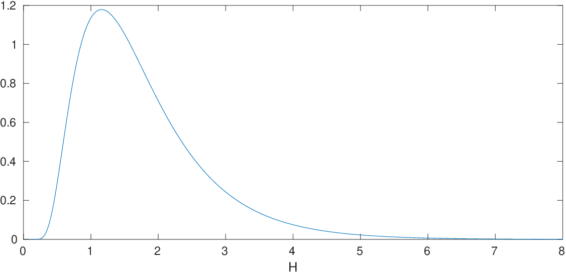
and, since I0′′​(0)=12I^{\prime\prime}_{0}(0)=\frac{1}{2}, we obtain that ∂x2,32u∗​(O)=∂r2u⁡(0,0)=λ>0\partial^{2}_{x_{2,3}}u^{*}(O)=\partial^{2}_{r}u(0,0)=\lambda>0, as expected. Figure 4 allows to understand the dependence of λ\lambda on the geometry of the cylinder.

Refer to caption
Figure 4: The quantity λ\lambda as a function of HH, the height of the cylinder, with a=1a=1.

References

  • [1] G. S. Alberti. On multiple frequency power density measurements. Inverse Problems, 29(11):115007, 25, 2013.
  • [2] G. S. Alberti. Enforcing local non-zero constraints in PDEs and applications to hybrid imaging problems. Comm. Partial Differential Equations, 40(10):1855–1883, 2015.
  • [3] G. S. Alberti. On multiple frequency power density measurements II. The full Maxwell’s equations. J. Differential Equations, 258(8):2767–2793, 2015.
  • [4] G. S. Alberti. Absence of Critical Points of Solutions to the Helmholtz Equation in 3D. Arch. Ration. Mech. Anal., 222(2):879–894, 2016.
  • [5] G. S. Alberti and Y. Capdeboscq. Lectures on elliptic methods for hybrid inverse problems. Technical Report 2016-46, Seminar for Applied Mathematics, ETH Zürich, Switzerland, 2016.
  • [6] G. S. Alberti and Y. Capdeboscq. On local non-zero constraints in PDE with analytic coefficients. In Imaging, Multi-scale and High Contrast Partial Differential Equations, volume 660 of Contemp. Math., pages 89–97. Amer. Math. Soc., Providence, RI, 2016.
  • [7] G. Alessandrini. An identification problem for an elliptic equation in two variables. Ann. Mat. Pura Appl. (4), 145:265–295, 1986.
  • [8] G. Alessandrini. Global stability for a coupled physics inverse problem. Inverse Problems, 30(7):075008, 10, 2014.
  • [9] G. Alessandrini, M. Di Cristo, E. Francini, and S. Vessella. Stability for quantitative photoacoustic tomographywith well-chosen illuminations. Annali di Matematica Pura ed Applicata (1923 -), pages 1–12, 2016.
  • [10] G. Alessandrini and R. Magnanini. Elliptic equations in divergence form, geometric critical points of solutions, and Stekloff eigenfunctions. SIAM J. Math. Anal., 25(5):1259–1268, 1994.
  • [11] G. Alessandrini and V. Nesi. Univalent σ\sigma-harmonic mappings. Arch. Ration. Mech. Anal., 158(2):155–171, 2001.
  • [12] H. Ammari. An Introduction to Mathematics of Emerging Biomedical Imaging, volume 62 of Mathematics and Applications. Springer, New York, 2008.
  • [13] H. Ammari, E. Bonnetier, Y. Capdeboscq, M. Tanter, and M. Fink. Electrical impedance tomography by elastic deformation. SIAM J. Appl. Math., 68:1557–1573, 2008.
  • [14] H. Ammari, J. Garnier, W. Jing, and L. H. Nguyen. Quantitative thermo-acoustic imaging: an exact reconstruction formula. J. Differential Equations, 254(3):1375–1395, 2013.
  • [15] A. Ancona. Some results and examples about the behavior of harmonic functions and Green’s functions with respect to second order elliptic operators. Nagoya Math. J., 165:123–158, 2002.
  • [16] S. R. Arridge and O. Scherzer. Imaging from coupled physics. Inverse Problems, 28:080201, 2012.
  • [17] G. Bal. Hybrid inverse problems and internal functionals. Inside Out II, MSRI Publications, G. Uhlmann Editor, Cambridge University Press, Cambridge, UK, 2012.
  • [18] G. Bal. Hybrid Inverse Problems and Redundant Systems of Partial Differential Equations. In P. Stefanov, A. Vasy, and M. Zworski, editors, Inverse Problems and Applications, volume 619 of Contemporary Mathematics, pages 15–48. AMS, 2014.
  • [19] G. Bal and M. Courdurier. Boundary control of elliptic solutions to enforce local constraints. J. Differential Equations, 255(6):1357–1381, 2013.
  • [20] G. Bal and K. Ren. On multi-spectral quantitative photoacoustic tomography. Inverse Problems, 28:025010, 2012.
  • [21] G. Bal and G. Uhlmann. Inverse diffusion theory for photoacoustics. Inverse Problems, 26(8):085010, 2010.
  • [22] G. Bal and G. Uhlmann. Reconstruction of coefficients in scalar second-order elliptic equations from knowledge of their solutions. Commun. Pure Appl. Math., 66:1629–1652, 2013.
  • [23] P. Bauman, A. Marini, and V. Nesi. Univalent solutions of an elliptic system of partial differential equations arising in homogenization. Indiana Univ. Math. J., 50(2):747–757, 2001.
  • [24] M. Briane, G. W. Milton, and V. Nesi. Change of sign of the corrector’s determinant for homogenization in three-dimensional conductivity. Arch. Ration. Mech. Anal., 173(1):133–150, 2004.
  • [25] L. A. Caffarelli and A. Friedman. Partial regularity of the zero-set of solutions of linear and superlinear elliptic equations. J. Differential Equations, 60:420�V433, 1985.
  • [26] G. Caloz, M. Dauge, and V. Péron. Uniform estimates for transmission problems with high contrast in heat conduction and electromagnetism. J. Math. Anal. Appl., 370(2):555–572, 2010.
  • [27] Y. Capdeboscq. On a counter-example to quantitative Jacobian bounds. J. Éc. polytech. Math., 2:171–178, 2015.
  • [28] Y. Capdeboscq, J. Fehrenbach, F. de Gournay, and O. Kavian. Imaging by modification: numerical reconstruction of local conductivities from corresponding power density measurements. SIAM J. Imaging Sciences, 2:1003–1030, 2009.
  • [29] L. C. Evans. Partial differential equations, volume 19 of Graduate Studies in Mathematics. American Mathematical Society, Providence, RI, 1998.
  • [30] D. Gilbarg and N. S. Trudinger. Elliptic partial differential equations of second order. Classics in Mathematics. Springer-Verlag, Berlin, 2001. Reprint of the 1998 edition.
  • [31] L. Grafakos. Modern Fourier analysis, volume 250 of Graduate Texts in Mathematics. Springer, New York, third edition, 2014.
  • [32] R. Hardt, M. Hoffmann-Ostenhof, T. Hoffmann-Ostenhof, and N. Nadirashvili. Critical sets of solutions to elliptic equations. J. Differential Geom., 51:359–373, 1999.
  • [33] D. Jerison and C. E. Kenig. The inhomogeneous Dirichlet problem in Lipschitz domains. J. Funct. Anal., 130(1):161–219, 1995.
  • [34] A. Jonsson and H. Wallin. Function spaces on subsets of 𝐑n{\bf R}^{n}. Math. Rep., 2(1):xiv+221, 1984.
  • [35] P. Kuchment. Mathematics of hybrid imaging: a brief review. In The mathematical legacy of Leon Ehrenpreis, volume 16 of Springer Proc. Math., pages 183–208. Springer, Milan, 2012.
  • [36] P. Kuchment and D. Steinhauer. Stabilizing inverse problems by internal data. Inverse Problems, 28(8):084007, 2012.
  • [37] G. Leoni. A first course in Sobolev spaces, volume 105 of Graduate Studies in Mathematics. American Mathematical Society, Providence, RI, 2009.
  • [38] V. G. Maz’ya and T. O. Shaposhnikova. Theory of Sobolev multipliers, volume 337 of Grundlehren der Mathematischen Wissenschaften [Fundamental Principles of Mathematical Sciences]. Springer-Verlag, Berlin, 2009. With applications to differential and integral operators.
  • [39] J. R. McLaughlin, N. Zhang, and A. Manduca. Calculating tissue shear modulus and pressure by 2D log-elastographic methods. Inverse Problems, 26(8):085007, 25, 2010.
  • [40] I. Mitrea and M. Mitrea. The Poisson problem with mixed boundary conditions in Sobolev and Besov spaces in non-smooth domains. Trans. Amer. Math. Soc., 359(9):4143–4182 (electronic), 2007.
  • [41] A. Nachman, A. Tamasan, and A. Timonov. Current density impedance imaging. Tomography and Inverse Transport Theory. Contemporary Mathematics (G. Bal, D. Finch, P. Kuchment, P. Stefanov, G. Uhlmann, Editors), 559, 2011.
  • [42] V. S. Rychkov. On restrictions and extensions of the besov and triebel–lizorkin spaces with respect to lipschitz domains. Journal of the London Mathematical Society, 60(1):237–257, 1999.
  • [43] O. Scherzer. Handbook of Mathematical Methods in Imaging. Springer Verlag, New York, 2011.
  • [44] T. Widlak and O. Scherzer. Hybrid tomography for conductivity imaging. Inverse Problems, 28(8):084008, 28, 2012.