A velocity tracking approach for the Data Assimilation problem in blood flow simulations

In this section we describe the numerical algorithm to solve (1-2). It is based on the Discretize then Optimize (DO) approach which consists of first discretizing the optimal control problem and then solving the optimization problem (finite dimensional) resulting from the discretization. An alternative approach is the adjoint (indirect) approach, or Optimize then Discretize (OD). For certain type of parabolic problems, [44] and [45] indicated that DO approach may be preferred. In [46] and [47], the authors pointed out that, in nonlinear problems, such us fluid control problems, OD could result in a discrete optimal solution failing to be optimal for the continuous problem. In [48], in the frame of stabilized advection equations, it was shown that both approaches can lead to different solutions, but, in certain cases, the OD has better asymptotic convergence properties. These conclusions were reinforced in [49]. Concerning the case of the Navier-Stokes equations, different perspectives were suggested. We refer to [50] for a DO approach in the frame of boundary control, and to [51] for a OD approach in the frame of distributed control. It appears that, at the present stage, no general answer can be given. In particular, concerning problem (1-2), this question remains without unanswered. In [37], where a pressure type control was considered, the authors obtained better performance of the DO, in terms of accuracy of the controlled solution. Based on these results, we have adopted here the DO approach. Nevertheless, a detailed comparison of these two approaches should be the subject of future research.

Let us assume that we are looking for ${\bf u}\in\mathbf{H}^{1}(\Omega)$ and for $p\in\mathbf{L}^{2}(\Omega)$. We consider ${\mathbf{V}=\{\mathbf{v}\in\mathbf{H}^{1}(\Omega):\ \mathbf{v}|_{\partial\Omega_{D}}=0\}}$, where $\partial\Omega_{D}=\Gamma_{in}\cup\Gamma_{wall}$, $\mathbf{Q}=\mathbf{L}^{2}(\Omega)$. Multiplying the first two equations of (1) by test functions $\mathbf{v}\in\mathbf{V}$ and $q\in\mathbf{Q}$, and integrating by parts, we obtain

which is the weak form of system (1). The symbol "$:$" represents the inner product of two second-order tensors.

To discretize problem (2)-(5) we consider $\mathbf{V}_{h}$ and $\mathbf{Q}_{h}$, subpaces of $\mathbf{V}$ and $\mathbf{Q}$, with finite dimensions $dim(\mathbf{V}_{h})=N_{u}$ and $dim(\mathbf{Q}_{h})=N_{p}$, respectively. We assume $\mathbf{V}_{h}$ and $\mathbf{Q}_{h}$ to represent spaces of Lagrange type Finite Elements, associated to a partition $\tau_{h}$ of $\Omega$. Therefore the dimensions $N_{u}$ and $N_{p}$ tend to infinity when $h$ tends to zero. A map between the nodes describing $\tau_{h}$ and the basis functions with dimensions both $\mathbf{V}_{h}$ and $\mathbf{Q}_{h}$ can be defined.

The discretized unknown variables are now given by

where $u_{j}$ and $p_{k}$ are unknown coefficients to be determined and $\phi_{j}$ and $\psi_{k}$ are the shape functions which form a basis of $\mathbf{V}_{h}$ and $\mathbf{Q}_{h}$, respectively.

Assuming that we can associate some basis functions $(\phi_{i})_{i=1...N_{o}}$ with the nodes in $\Omega_{part}$, and some others to the nodes on $\Gamma_{in}$, which we refer to as $(\phi_{i})_{i=1...N_{g}}$, we then approximate the control function in (2) as

We assume also that ${\bf u}_{d}$ can be approximated by

Let us begin by discretize the cost functional $J$ given by (2). The first term of $J$ becomes

where $\|\cdot\|_{N_{o}}$ is the norm induced by the inner product $(\cdot,\cdot)_{M}$ and ${M}$ is a symmetric $N_{o}\times N_{o}$ matrix where each element is given by

For the regularization term we have

where $\|\cdot\|_{A}$ is the norm induced by the inner product $(\cdot,\cdot)_{A}$. Matrix ${A}$ is a symmetric $N_{g}\times N_{g}$ matrix whose elements are defined by

where ":" represents the inner product of two second-order tensors.

Then, the discretized form of the cost functional (2) becomes:

With respect to system (5), to deal with convected dominated regimes, a GLS (Galerkin-Least-Squares) stabilization (see [52]) is adopted here. To describe it, let us first consider

and

Using this notation, the stabilized version of (5) consists of finding ${\bf u}_{h}\in\mathbf{V}_{h}$ and $p_{h}\in\mathbf{Q}_{h}$ such that

where ${\cal{L}}^{1}_{h}$ and ${\cal{L}}^{2}_{h}$ are defined by

and

so that ${\cal{L}}^{1}_{h}$ verifies

Here $\tau_{h}$ represents a partition of $\Omega$ with characteristic length $h$, $\lambda$ is a penalty parameter (see [53]) and $L$ and $\varphi$ are given by

The parameter $\delta$ should be suitably chosen. In this work, the parameter is taken from [54] (see [55] for more details). Notwithstanding, $\delta$ can be optimized in the frame of optimal control problems ([48] and [56]).

In order to obtain the discretization of system (10), let us first discretize the convective term of $a({\bf u}_{h},{\bf v}_{h})$ and its counterpart in ${\cal{L}}^{1}_{h}({\bf u}_{h},{\bf f},{\bf v}_{h})$:

Using the approximations (6) and after some computations, the above expression can be written as

where ${\bf U}=(u_{1},...,u_{N_{u}})^{T}$ and ${{N}}({\bf U})$ and ${\cal{N}}({\bf U})$ are matrices whose elements are defined by

We now turn our attention to the diffusion term:

Replacing ${\bf u}_{h}$ by its corresponding finite approximation we can write

where

Acting similarly for the pressure term, we obtain for the first equation in (10),

where

as for ${\cal L}_{h}^{2}$, we consider

which, by replacing $p_{h}$ by it�s corresponding finite approximation, gives

Hence, adding the discretized terms of ${\cal L}_{1}$ and ${\cal L}_{2}$, system (10) becomes

where

We remark that vector ${\bf U}=({\bf U}_{g},{\bf G})$ includes the controlled velocity coefficients ${\bf G}$ and the uncontrolled ones ${\bf U}_{g}$ which also depend on ${\bf G}$. Therefore, the stabilized problem can be recast into the general form

where (14) represents the problem constraints (12), including boundary conditions. In spite of (13-14) being finite dimensional, it is a large scale optimization problem with nonlinear constraints and a quadratic cost. To solve this problem, we use the Sequential Quadratic Programming algorithm, as described in [57]. The algorithm is available in the SNOPT library ([58]) and was tested in several benchmark large scale problems. The iterative procedure requires the evaluation of $F({\bf G})$ which, in turn, implies solving the nonlinear system (12). To solve it, the damped Newton method - as described in [59] - was used.

We will now briefly describe the algorithm and we refer to [57], for more details.

Let us assume that the solution ${\bf G}$ of (13)-(14) verifies the Karush-Kuhn-Tucker (KKT) optimality conditions

where $\mathcal{D}F$ and $\mathcal{D}C$ are the gradients of $F$ and $C$, respectively, and $\lambda$ is the vector of the Lagrange multipliers. If one is able to find a good initial estimate ${\bf G}_{0}$ (and corresponding $\lambda_{0}$), close enough to the optimal ${\bf G}$, the following algorithm produces a sequence that is globally convergent ([57]).

We remark that step 2 of Algorithm 1, which concerns the solution of the linear quadratic problem, is conducted using the library SQOPT ([61]).

As mentioned at the end of Section I, one of the questions we would like to address is how our approach compares to the approach based on a Neumann control ([37]). To this end, we started by reproducing the results there presented for an idealized 2D straight channel $\Omega=[0,5]\times[-0.5,0.5]$ with $\Gamma_{in}=\{0\}\times[-0.5,0.5]$ and $\Gamma_{out}=\{5\}\times[-0.5,0.5]$. The observations were assumed to correspond to the sections $\{1\}\times[-0.5,0.5]$, $\{2.5\}\times[-0.5,0.5]$ and $\{4\}\times[-0.5,0.5]$. Taking $\nu=1$, we considered the ground truth solution to be known exactly and given by ${\bf u}=1-4y^{2}$ (in particular ${\bf u}=0$ on $\Gamma_{wall}=\partial\Omega\setminus(\Gamma_{in}\cup\Gamma_{out})$. As mentioned above, in [37], the authors considered the problem of controlling a boundary condition of type (3). We refer to this procedure as solving problem (P2), by opposition to solving problem (1-2), to which we refer as (P1). We remark that while in (P1) the control is a vector function (2D), in (P2) it is a scalar function. Thus, to solve (P2), the cost function should be properly rewritten, and Algorithm 1 may then be applied in a similar way. In [37], the weights in the cost function were set to be $\beta_{1}=\frac{1}{2}$ and $\beta_{2}=\frac{10^{-9}}{2}$, accordingly to the Morozov Discrepancy Principle associated to a certain fixed signal-to-noise ratio (see, for instance, [60]). Since we were interested in comparing specifically the role of the control nature in the results, we did not include - in this section - any noise on the observations.

To solve (P2), as described above, we fixed a Neumann homogeneous condition at $\Gamma_{out}$ and we considered $P_{2}-P_{1}$, the usual Lagrange linear FEM corresponding to 27K degrees of freedom (maximum element size $h=1/20$) for the velocity. The assembly of the FEM matrices required to obtain the equivalent to system (12) was done with COMSOL Multiphysics ([62]). Since, at this stage, the Reynolds number was very small, the matrices corresponding to the convective and stabilization terms were neglected. To solve the linearized systems at the iteration level, the PARDISO library was used. The result gave a controlled solution that approximates the exact solution with a relative error of 0$.00112$, that is, of order $\approx 0.1\%$. Correspondingly to the conclusions in [37], this means that the Neumann control was able to successfully adjust the solution to the data. For this reason, we used this percentage as the reference relative error to fix the weights $\beta_{1}$ and $\beta_{2}$ in our comparative example - which will be described next.

We considered the previous domain and extended it to obtain the curved vessel represented in Figure 2 (left). We will refer to this extended domain as the ground truth domain. As it is well known ([4]), in a straight channel, even for at physiological Reynolds numbers, pressure contours tend to remain parallel to the cross sections of the computational domain. In a curved vessel, however, that is no longer true, even for Reynolds numbers bellow typical physiologic values.

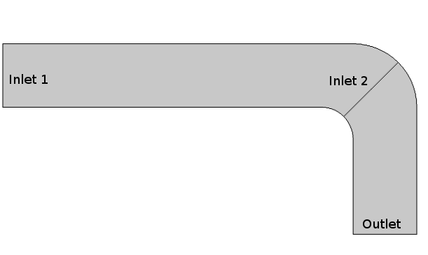
To illustrate this, fixed the same model as before, but we slightly increased the Reynolds number by considering a parabolic profile $10(1-4^{2})$ at inlet 1. We then solved system (1) to obtain the ground truth solution ${\bf u}_{d}$. As the Reynolds number was now higher, we considered all the terms in system (12), including the stabilizing terms. An unstructured mesh corresponding to 43K degrees of freedom (max $h=1/20$) was used. The nonlinear system was solved using the damped Newton’s method, as mentioned in Section II. The ground truth solution is represented in Figure 3. We can see that the pressure contours are no long parallel to cross sections within the curve, and the velocity profile loses the parabolic shape on those cross sections.

Our aim next was to mimic a more realistic situation, where the unknown inlet boundary condition did not correspond to a parabolic velocity profile, normal at $\Gamma_{in}$, nor to a pressure profile, that could be assumed axial dependent. For this reason, we truncated the channel at the section labeled inlet 2, which became the new artificial inlet of the shorter domain represented in Figure 2(right). We call this domain $\Omega$ and its inlet boundary $\Gamma_{in}$. Therefore, we put ourselves into the scenario where we would like to fix a boundary condition at $\Gamma_{in}$ so that the solution in the shorter domain $\Omega$ would match, as much as possible, the ground truth solution ${\bf u}_{d}$. For the observations, we assumed to have measured exactly the velocity profiles of the true solution ${\bf u}_{d}$ at $\Omega_{part}=S1\cup S2\cup S3$, where $S1$, $S2$ and $S3$ are lines that were chosen arbitrarily inside $\Omega$ (Figure 2, left). Before solving both problems (P1) and (P2), we needed to set $\beta_{1}$ and $\beta_{2}$. Following what was done above, concerning the example in [37], we fixed $\beta_{1}=\frac{1}{2}$ and we looked for $\beta_{2}$ so that a relative error

verifies $RE_{\Omega_{part},\beta_{2}}\approx 0.00112$. In the expression of the relative error, ${\bf u}_{\beta_{2}}$ represents the solution of the control problem associated to $\beta_{2}$. We did this by heuristically fixing a sample for $\beta_{2}$ and evaluating the corresponding relative errors obtained using Algorithm 1 with an optimality tolerance of $10^{-6}$. The results are shown in Figure 4 and Table 1.

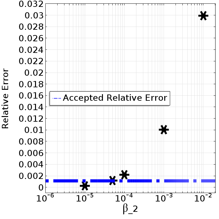
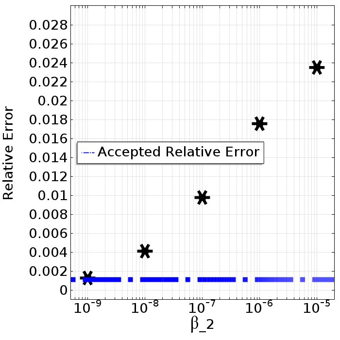
From these conclusions we fixed $\beta_{2}=2.5\times{10^{-5}}$ for (P1) $\beta_{2}=0.5\times{10^{-9}}$ for (P2).

The solutions obtained for (P1) and (P2) are represented in the second row of Figure 5, and first row of Figure 6, respectively.

The results show that the solution obtained with the velocity control is qualitatively closer to the ground truth solution, represented in the first row of Figure 5. To quantify these different performances, we use the relative error of the controlled solutions with respect to ${\bf u}_{d}$, evaluated at different sites. In Table 2 we present the values for

where $\|\cdot\|_{\mathbf{L}^{2}(\Omega)}$ is the $\mathbf{L}^{2}(\Omega)$ norm, and for $RE_{\Gamma_{in}}$ and $RE_{\Omega_{part}}$, which are computed analogously. We also indicate the final value for the cost functional and the number of cost evaluations. It can be seen that, while a relative error on the observations site is kept on the same order, the solution of (P1) is globally more near to ${\bf u}_{d}$ than the solution of (P2). Actually, looking closer to the later pressure profile (Figure 6, 1st row), some oscillations can be seen at the inlet. This indicates that, although the relative error on the observations was of order $0.1\%$, the weight $\beta_{2}=0.5\times 10^{-9}$ almost neglected the regularizing effect of the second term in the cost function. An increase in $\beta_{2}$ improves the regularizing effect, but at the expenses of distancing from the desired relative error. We illustrate this by considering the case (P2r) with $\beta_{2}=0.5\times 10^{-6}$, for which the results are shown in Table 2 and in the second row of Figure 6.

These results indicate that, if the accuracy of the numerical solution is our aim, in some scenarios - like the one just illustrated - a velocity control approach can be more convenient. A higher number of cost evaluations might however be required. Such conclusion does not invalidates the fact that (P2) is prone to perform well, when pressure contours align with cross section in the region close to the inlet, as shown in [37] and [38].

Next, we assessed the convergence of the solution pair $(\mathbf{u},\mathbf{g})$ with respect to mesh refinement. We considered the desired solution as the one obtained by solving (P1) with a maximum mesh size of $h=1/80$. Then, we computed the relative errors both control and velocity solutions, which we represent in Figure 7. The convergence test resulted positive.

Until now, (P1) was only solved for small Reynolds numbers. This allowed us to illustrate the advantages of velocity control, while remaining close to the example analyzed in [37]. These Reynolds numbers were still far for common physiologic values found in the cardiovascular system. To explore the robustness with respect to such values, we solved (P1) for increasing Reynolds numbers. The results are presented in Table 3. We can see that the number of iterations, required to solve Algorithm 1, increases significantly with the Reynolds number. Also, since we kept the weights $\beta_{1}$ and $\beta_{2}$ fixed, there is an increase of the relative error on the observations site $\Omega_{part}$. Naturally, this error propagates to the rest of the solution. To keep the relative error within acceptable values, let say, around $0.1\%$, we need to adjust the weight parameters, as it was done above. To illustrate this, we show the results obtained by considering $\beta_{2}=0.1\times 10^{-5}$ in Table 4. We can see that with these parameters the relative errors can be of order $0.1\%$.

In this section we present the numerical results found after applying the DA approach (P1) to a realistic geometry obtained from the segmentation of Computed Tomography (CT) data sets of a saccular brain aneurysm.

As in the previous example, we used an extended ground truth domain to computed the ground solution ${\bf u}_{d}$. This solution was used both to select the measured data and to estimate the accuracy of the method. The ground truth domain is represented in Figure 8 (left). For the model parameters, we considered $\nu=\frac{\mu}{\rho}$ with $\mu=3.67\times 10^{-3}\,Pa.s$, a value within the range suggested in [22]. Also, we took $\rho=1050\,Kg/m^{3}$ and we fixed a laminar inflow profile - normal to the inlet - which corresponds to a flow rate of $Q=4\times 10^{-6}m^{3}/s$. Again, these are typical parameters used for blood flow simulations (see [22]). At the inlet this values implied a physiological Reynolds number of $367$. No slip boundary conditions were imposed on the vessel wall and zero normal stress (Neumann homogeneous) was fixed on the outflow boundary. To obtain system 12 and for its numerical solution we adopted the same choices as in the previous example, except that P1-P1 finite elements were used instead. We remark that the system was stabilized using GLS.

First, we analyzed the case when the same degrees of freedom were used both to generate ${\bf u}_{d}$ and for the DA procedure. Subsequently, the ground truth solution was generated using a finer mesh. The second scenario was considered in order to avoid the so called inverse crime problem. This is the case when the same model and discretization are used both to generate the synthetic data - from where the observations are chosen - and to solve the control (inverse) problem. Indeed, some particular inverse crime problems can have a trivial solution ([63]). Although this is not necessarily the case for fluid control problems (see, for instance, [46] and [47] for some simple examples with non-trivial solution), we still distinguish between both scenarios. Thus, we can change the observed data either by generating it using a different (finer) mesh, adding noise to it, or both, as we have done it this study.

References

- [1] Blanco PJ, Watanabe SM, Passos MA, Lemos PA, Feijóo RA. An anatomically detailed arterial network model for one-dimensional computational hemodynamics. IEEE Transactions on Biomedical Engineering 2015; 62(2):736-53.
- [2] Formaggia L, Nobile F, Quarteroni A, Veneziani A. Multiscale modelling of the circulatory system: a preliminary analysis. Computing and Visualization in Science 1999; 2:75-83.
- [3] Grinberg L, Anor T, Madsen JR, Yakhot A, Karniadakis GE. Large-scale simulation of the human arterial tree. Clinical and Experimental Pharmacology and Physiology 2009; 36(2):194-205.
- [4] Quarteroni A, Veneziani A, Vergara C. Geometric multiscale modeling of the cardiovascular system, between theory and practice. Computer Methods in Applied Mechanics and Engineering 2016; 302:193–252.
- [5] DeVault K, Gremaud PA, Novak V, Olufsen MS, Vernieres G, Zhao P. Blood flow in the circle of Willis: modeling and calibration. Multiscale Modeling & Simulation 2008; 7(2):888-909.
- [6] Ismail M, Wall WA, Gee MW. Adjoint-based inverse analysis of windkessel parameters for patient-specific vascular models. Journal of Computational Physics 2013; 244:113-130.
- [7] Lombardi D. Inverse problems in 1D hemodynamics on systemic networks: A sequential approach. International Journal for Numerical Methods in Biomedical Engineering 2014; 30(2):160-179.
- [8] Pant S, Fabreges B, Gerbeau JF, Vignon-Clementel IE. A methodological paradigm for patient-specific multi-scale cfd simulations: from clinical measurements to parameter estimates for individual analysis. International Journal for Numerical Methods in Biomedical Engineering 2014; 30(12):1614-1648.
- [9] Formaggia L, Gerbeau JF, Quarteroni A. Numerical Treatment of Defective Boundary Conditions for the Navier–Stokes Equations. SIAM Journal on Numerical Analysis 2002; 40(1):376-401.
- [10] Kim HJ, Figueroa CA, Hughes TJR, Jansen KE, Taylor CA. Augmented Lagrangian method for constraining the shape of velocity profiles at outlet boundaries for three-dimensional finite element simulations of blood flow. (English summary), Computer Methods in Applied Mechanics and Engineering 2009; 198(45-46): 3551-3566.
- [11] Balossino R, Pennati G, Migliavacca F, Formaggia L, Veneziani A, Tuveri M, Dubini G. Computational models to predict stenosis growth in carotid arteries: Which is the role of boundary conditions? Computer Methods in Biomechanics and Biomedical Engineering 2009; 12:113-123. /doi/abs/10.1137/S003614290038296X.
- [12] Wake AK1, Oshinski JN, Tannenbaum AR, Giddens DP. Choice of in vivo versus idealized velocity boundary conditions influences physiologically relevant flow patterns in a subject-specific simulation of flow in the human carotid bifurcation. Journal of Biomechanical Engineering 2009; 131(2):021013. doi: 10.1115/1.3005157.
- [13] Oshima M, Sakai H, Torii R. Modelling of Inflow Boundary Conditions for Image-based Simulation of Cerebrovascular Flow. International Journal for Numerical Methods in Fluids 2005; 47(6-7):603-617.
- [14] Castro MA, Putman CM, Cebral JR. Computational fluid dynamics modeling of intracranial aneurysms: effects of parent artery segmentation on intra-aneurysmal hemodynamics. American Journal of Neuroradiology 2006; 27(8): 1703-1709.
- [15] Jansen IG, Schneiders JJ, Potters WV, van Ooij P, van den Berg R, van Bavel E, Marquering HA, Majoie CB. Generalized versus patient-specific inflow boundary conditions in computational fluid dynamics simulations of cerebral aneurysmal hemodynamics. American Journal of Neuroradiology 2014; 35(8):1543-1548.
- [16] Marzo A, Singh P, Reymond P, Stergiopulos N, Patel U, Hose R. Influence of inlet boundary conditions on the local haemodynamics of intracranial aneurysms. Computer Methods in Biomechanics and Biomedical Engineering 2009; 12(4):431-44.
- [17] Campbell IC1, Ries J, Dhawan SS, Quyyumi AA, Taylor WR, Oshinski JN. Effect of inlet velocity profiles on patient-specific computational fluid dynamics simulations of the carotid bifurcation. Journal of Biomechanical Engineering 2012; 134(5):051001.
- [18] Moyle KR, Antiga L, Steinman DA. Inlet Conditions for Image-Based CFD Models of the Carotid Bifurcation: Is it Reasonable to Assume Fully Developed Flow?. Journal of Biomechanical Engineering 2006; 128(3):371-379.
- [19] Fasano A, Pavlova J, Sequeira A. Numerical simulations of a reduced model for blood coagulation. Zeitschrift für angewandte Mathematik und Physik 2016; 67:28 DOI: 10.1007/s00033-015-06010-2.
- [20] Cilla M, Pena E, Martinez M. Mathematical modelling of atheroma plaque formation and development in coronary arteries. Journal of The Royal Society Interface 2013; 11(90):20130866.
- [21] Santos R, Sequeira A, Silva T, Tiago J. Existence, uniqueness, stability and asymptotic behavior of solutions for a mathematical model of atherosclerosis. Discrete and Continuous Dynamical Systems - Series S 2016; 9(1):343-362.
- [22] Gambaruto A, Janela J, Moura A, Sequeira A. Sensitivity of hemodynamics in a patient specific cerebral aneurysm to vascular geometry and blood rheology. Mathematical Biosciences and Engineering 2011; 8(2):409-423.
- [23] Cebral JR, Castro MA, Appanaboyina S, Putman CM, Millan D, Frangi AF. Efficient pipeline for image-based patient-specific analysis of cerebral aneurysm hemodynamics: Technique and sensitivity. IEEE Transactions in Medical Imaging 2005; 24(4):457-467.
- [24] Morbiducci U1, Ponzini R, Rizzo G, Cadioli M, Esposito A, De Cobelli F, Del Maschio A, Montevecchi FM, Redaelli A. In vivo quantification of helical blood flow in human aorta by time-resolved three-dimensional cine phase contrast magnetic resonance imaging. Annals of Biomedical Engineering 2009; 37(3):516-531.
- [25] den Reijer PM1, Sallee D 3rd, van der Velden P, Zaaijer ER, Parks WJ, Ramamurthy S, Robbie TQ, Donati G, Lamphier C, Beekman RP, Brummer ME. Hemodynamic predictors of aortic dilatation in bicuspid aortic valve by velocity-encoded cardiovascular magnetic resonance. Journal of Cardiovascular Magnetic Resonance 2010; 12:4 doi: 10.1186/1532-429X-12-4.
- [26] Onishi Y1, Aoki K, Amaya K, Shimizu T, Isoda H, Takehara Y, Sakahara H, Kosugi T. Accurate determination of patient-specific boundary conditions in computational vascular hemodynamics using 3D cine phase-contrast MRI. International Journal for Numerical Methods in Biomedical Engineering 2013; 29(10):1089-1103.
- [27] Wang B, Zou X, Zhu J. Data assimilation and its applications. Proc. Natl. Acad. Sci. USA, 2000; 97(21):11143-11144.
- [28] Moireau P, Bertoglio C,Xiao N, Figueroa C A, Taylor C A, Chapelle D, Gerbeau J F, Sequential identification of boundary support parameters in a fluid-structure vascular model using patient image data. Biomechanics and Modeling in Mechanobiology 2013; 12(3):475-496.
- [29] Bertagna L, Veneziani A, A model reduction approach for the variational estimation of vascular compliance by solving an inverse fluid-structure interaction problem. Inverse Problems 2014; 30(5) 055006.
- [30] Schiavazzi D E, Arbia G, Baker C, Hlavacek A M, Hsia T Y, Marsden A L, Vignon-Clementel I E, "Uncertainty quantification in virtual surgery hemodynamics predictions for single ventricle palliation," International Journal for Numerical Methods in Biomedical Engineering 2016; 32(3):e02737.
- [31] Marsden A. Optimization in Cardiovascular Modeling. Annual Review of Fluid Mechanics 2014; 46:519-546.
- [32] Bertagna L, D’Elia M, Perego M, Veneziani A. Data assimilation in cardiovascular fluid-structure interaction problems: an introduction. Fluid-structure interaction and biomedical applications. Advances in Mathematical Fluid Mechanics 2014; 395-481.
- [33] Formaggia L, Veneziani A, Vergara C. A new approach to numerical solution of defective boundary value problems in incompressible fluid dynamics. SIAM Journal on Numerical Analysis 2008; 46(6): 2769-2794.
- [34] Formaggia L, Veneziani A, Vergara C. Flow rate boundary problems for an incompressible fluid in deformable domains: Formulations and solution methods. Computer Methods in Applied Mechanics and Engineering, 2010; 199(9-�12): 677-688.
- [35] Heys JJ, et al., Weighted least-squares finite elements based on particle imaging velocimetry data. Journal of Computational Physics 2010; 229(1):107-118.
- [36] Rajaraman PK, Manteuffel TA, Belohlavek M, McMahon E, Heys JJ. Echocardiographic particle imaging velocimetry data assimilation with least square finite element methods. Computers and Mathematics with Applications 2014; 68(11):1569-1580.
- [37] D’Elia M, Veneziani A. Methods for assimilating blood velocity measures in hemodynamics simulations: preliminary results. Procedia Computer Science 2010; 1(1):1225-1233.
- [38] D’Elia M, Perego A, Veneziani A. A Variational Data Assimilation Procedure for the Incompressible Navier-Stokes Equations in Hemodynamics. Journal of Scientific Computing 2011; 52(2):340-359.
- [39] D’Elia M, Veneziani A. Uncertainty quantification for data assimilation in a steady incompressible Navier-Stokes problem.ESAIM: Mathematical Modelling and Numerical Analysis 2013; 47(4):1037-1057.
- [40] Guerra T, Tiago J, Sequeira A. Optimal control in blood flow simulations. International Journal of Non-Linear Mechanics 2014; 64:57-69.
- [41] Formaggia L, Quarteroni A, Veneziani A. The circulatory system: from case studies to mathematical modelling, in Complex Systems in Biomedicine, A. Quarteroni, L. Formaggia and A. Veneziani Eds., Springer, Milan, 243-287, 2006.
- [42] Robertson AM, Sequeira A, Kameneva M. Hemorheology. Hemodynamical Flows. Modeling, Analysis and Simulation, 37, 63-120, Birkhauser Verlag Basel Switzerland, 2008.
- [43] Guerra T, Sequeira A, Tiago J. Existence of optimal boundary control for Navier-Stokes with mixed boundary conditions, Portugaliae Mathematica 2015; 72(2-3):267-283.
- [44] Betts JT, Campbell SL, Discretize Then Optimize, Technical Document Series, &CT-TECH-03-01, Mathematics and Computing Technology, Phantom Works, Boeing, Seattle, 2003.
- [45] Hinze M, Tr¨oltzsch F. Discrete concepts versus error analysis in PDE-constrained optimization GAMM-Mitt; 2010 33( 2): 148-162.
- [46] Burkardt J, Gunzburger M, Peterson J. Insensitive functionals, inconsistent gradients, spurious minima and regularized functionals in flow optimization problems. International Journal of Computational Fluid Dynamics 2002; 16(3):171-185.
- [47] Gunzburger M, Perspectives in Flow Control and Optimization. SIAM, 2003.
- [48] Collis S, Heinkenschloss M. Analysis of the Streamline Upwind/Petrov Galerkin Method Applied to the Solution of Optimal Control Problems Tech Rep TR02-01. DCAM Rice University, Houston Tx March 2002.
- [49] Heinkenschloss M, Leykekhman D. Local Error Estimates for SUPG Solutions of Advection-Dominated Elliptic Linear-Quadratic Optimal Control Problems. SIAM Journal on Numerical Analysis; 47(6): 4607-4638.
- [50] Gunzburger M, Manservisi S. The velocity tracking problem for Navier-Stokes flows with boundary control. SIAM Journal on Control and Optimization 2000; 39:594-634.
- [51] Deckelnick K, Hinze, M. Semidiscretization and error estimates for distributed control of the instationary Navier-Stokes equations. Numerische Mathematik 2004; 97(2): 297-320.
- [52] G. Hauke G, Hughes TJR. A unified approach to compressible and incompressible flows, Computer Methods in Applied Mechanics and Engineering 1994;113: 389-395.
- [53] Brooks A, Hughes THJ. Streamline Upwind/Petrov-Galerkin Formulations for a Convection Dominated Flows with a Particular Emphasis on the Incompressible Navier-Stokes Equations. Computer Methods in Applied Mechanics and Engineering 1982; 32:199-259.
- [54] Bazilevs Y, Calo V, Tezduyar T, Hughes T. YZ discontinuity capturing for advection-dominated processes with application to arterial drug delivery. Int. J. Numer. Meth. Fluids 2007 54:593-608.
- [55] Shakib F, Hughes T, Zdenk J. A new finite element formulation for computational fluid dynamics: X. The compressible Euler and Navier-Stokes equations. Computer Methods in Applied Mechanics and Engineering 1991 89:141-219.
- [56] Abraham F, Behr M, Heinkenschloss M. The effect of stabilization in finite element methods for the optimal boundary control of the Oseen equations. Finite Elements in Analysis and Design 2003, 41:229-251.
- [57] Gill P, Murray W, Saunders MA. SNOPT: An SQP Algoritm for Large-Scale Constrained Optimization. SIAM REVIEW 2005 47(I): 99-131.
- [58] Gill P, Murray W, Saunders MA. User’s guide for SNOPT Version 7: Software for Large-Scale Nonlinear Programming, 2008.
- [59] Deuflhard P. A Modified Newton Method for the Solution of Ill-conditioned Systems of Nonlinear Equations with Application to Multiple Shooting. Numer. Math. 1974 22:. 289-315.
- [60] Ito K, Kunisch K. On the choice of the regularization parameter in nonlinear inverse problems. SIAM Journal on Optimization. 1992; 2(3):376-404.
- [61] Gill P, Murray W, Saunders WA, User’s guide for SQOPT Version 7: Software for large-scale linear and quadratic programming, Numerical Analysis Report 06-1, Department of Mathematics, University of California San Diego, La Jolla, CA, 2006.
- [62] COMSOL Multiphysics, Users Guide, COMSOL 4.3, 2012.
- [63] Kaipio J, Somersalo E. Statistical and Computational Inverse Problems, vol. 160, Applied Mathematical Sciences, Springer-Verlag, New York, 2005.