A generalized volume law for entanglement entropy
on the fuzzy sphere
Mariko Suzuki**
*
e-mail address :
f5344003@gmail.com
and
Asato Tsuchiya††
†
e-mail address : tsuchiya.asato@shizuoka.ac.jp
Department of Physics, Shizuoka University
836 Ohya, Suruga-ku, Shizuoka 422-8529, Japan
Graduate School of Science and Technology, Shizuoka University
3-5-1 Johoku, Naka-ku, Hamamatsu 432-8011, Japan
We investigate entanglement entropy in a scalar field theory on the fuzzy sphere. The theory is realized by a matrix model. In our previous study, we confirmed that entanglement entropy in the free case is proportional to the square of the boundary area of a focused region. Here we argue that this behavior of entanglement entropy can be understood by the fact that the theory is regularized by matrices, and further examine the dependence of entanglement entropy on the matrix size. In the interacting case, by performing Monte Carlo simulations, we observe a transition from a generalized volume law, which is obtained by integrating the square of area law, to the square of area law.
1 Introduction
It is widely recognized that noncommutative field theories are deeply connected to quantum gravity and string theory. On the other hand, since the discovery of the Ryu-Takayanagi formula [1], the connection between geometry and quantum entanglement has been revealed. One can, therefore, expect to gain insight into quantum gravity by studying quantum entanglement in noncommutative field theories.
Indeed, by studying a gravity dual of noncommutative super Yang-Mills theory (NCSYM) proposed in [2, 3], it was conjectured in [4, 5] that entanglement entropy (EE) in NCSYM is proportional to the volume of a focused region when the volume is small and to the area of the boundary of the region when the volume is large. While EE is proportional to the area in ordinary local field theories, the above volume law in NCSYM would originate from the UV/IR mixing [6] due to nonlocal interactions. Indeed, in [7], the volume law for EE is obtained in nonlocal theories.
In this paper, we use the words “volume” and “area” for real area and length, respectively, on a sphere. In [8, 9]11 1 For earlier studies, see [10, 11]., EE in a scalar field theory on the fuzzy sphere was studied at zero temperature in the free case22 2 Throughout this paper, the case where the action consists of only quadratic terms is called the “free case”, while the case where the action includes higher order terms is called the “interacting case”.. In [12], Okuno and the present authors reported the results for EE in the above theory. We verified that EE on the fuzzy sphere in the free case is proportional to the square of the area of the boundary, which was suggested in [9]. Moreover, we showed the first Monte Carlo results33 3 For Monte Carlo studies concerning the fuzzy sphere, see [13, 14, 15, 16, 17, 18]. for the interacting case, where we found that the behavior of EE is quite different from that in the free case. We also found that the finite temperature effect is governed by the volume law in the interacting case as well as in the free case. In calculating EE, we used a method that is different from the one in [8, 9]. This method was developed in [19] and used in [19, 20, 21].
In this paper, we continue the study of EE in the scalar field theory on the fuzzy sphere. We present further results for the free case as well as for the interacting case. In the free case, we discuss why EE obeys the square of area law, and further examine the dependence of EE on the matrix size. By performing Monte Carlo simulations in the interacting case, we observe a transition from a generalized volume law, which corresponds to the integral of the square of the area, to the square of area law, when the volume of a focused region is increased. This phenomenon would be attributed to the UV/IR anomaly discovered in [22, 23], which is the counterpart of the UV/IR mixing in field theories on compact noncommutative manifolds.
Another aim of our work is to elucidate geometry in matrix models. This is in particular important in the context of the study of matrix models proposed as nonperturbative formulation of string theory [24, 25, 26]. Indeed, the above scalar field theory on the fuzzy sphere is realized in a matrix model as a regularized theory. Following a prescription given in [8, 9], we divide the matrices into two parts, each one corresponding to one of the two regions on the sphere. We would like to see how well this division in the matrix works.
This paper is organized as follows. In section 2, we review a matrix model that realizes a scalar field theory on fuzzy sphere. In section 3, we describe how we calculate EE in this theory. We present the results for EE in the free case in section 4 and in the interacting case in section 5, respectively. Section 6 is devoted to conclusion and discussion.
2 Scalar field theory on the fuzzy sphere
2.1 Scalar field theory on the fuzzy sphere realized by a matrix model
The commutative counterpart of the noncommutative scalar field theory we consider in this paper is defined on as
| (2.1) |
where is the radius of , is the invariant measure for unit sphere, is the circumference of that corresponds to inverse temperature, and the dot stands for the derivative with respect to that parametrizes . (i=1,2,3) are the orbital angular momentum operators given by
| (2.2) |
To obtain the noncommutative field theory, we replace with the fuzzy sphere in (2.1). The resultant theory is realized by a matrix model, that is defined by
| (2.3) |
where is a nonnegative integer or a positive half-integer specifying the spin of the representation of , and is a Hermitian matrix that depends on . are the generators of the SU(2) algebra for the spin representation, and obey the relation .
Throughout this paper, we are concerned with the so-called commutative limit where with fixed. As stated below, the theory (2.3) agrees with the theory (2.1) at tree level in this limit, but differs from it with radiative corrections. The UV cutoff is given by . To see the correspondence between the two theories, it is convenient to introduce the Bloch coherent states ) [27]44 4 See also [28, 29, 30, 31]., which are localized around a point on the unit sphere. The properties of the Bloch coherent state are summarized in appendix A in [12].
The explicit form of is given by
where and are the standard basis for the spin representation of the SU(2) algebra satisfying
| (2.6) |
By using (2.1), it is easy to show that
| (2.7) |
and
| (2.8) |
where and . (2.8) implies that the width of the Bloch coherent state is given by .
We also introduce the Berezin symbol [32] defined by , which is identified with in (2.1) in the limit. First, by using (2.1), it can easily be shown that
| (2.9) |
Second, the star product for the two Berezin symbols is defined by
| (2.10) |
where (2.7) is used. The star product coincides with the ordinary one at the tree level in the limit, while it gives rise to the UV/IR anomaly at the quantum level. Indeed, the noncommutative parameter is given by [8, 30], which vanishes in the limit. Third, by using (2.7), the trace over a matrix is translated into the integral over . In this manner, the theory (2.3) coincides with the theory (2.1) at the tree level in the limit, while it differs from the theory (2.1) at the quantum level even in the limit due to the UV/IR anomaly. The length scale of nonlocality of the interaction that gives rise to the UV/IR anomaly is given by .
2.2 Division of the fuzzy sphere
Following the prescription in [8], we divide the fuzzy sphere into two regions.
First, let us see the relationship between the Berezin symbol and the matrix elements . We have a relation
| (2.11) |
By using (2.1), we find that
| (2.12) |
It is easy to show that (2.12) has a sharp peak at [8]
| (2.13) |
with width . This observation shows that the matrix elements correspond to the field at [8].
Next, using the relation (2.13), we assign regions A and B on the sphere in Fig.1(a) to parts A and B, respectively, of the matrix in Fig.1(b). In order to parametrize region A on the sphere, we introduce a parameter , which is the “volume” of the region A divided by :
| (2.14) |
Note that the “area” of the boundary between the regions A and B is given by
| (2.15) |
The condition that the element is located in part A is given by
| (2.16) |
where . From (2.13), (2.14) and (2.16), we find that
| (2.17) |

We can put without loss of generality. In the following sections, we further put for simplicity, and denote the matrix size by .
3 Calculation of EE
3.1 Entanglement entropy
The division of the matrix in Fig.1(b) corresponds to decomposing the Hilbert space in the theory (2.3) to a tensor product
| (3.1) |
EE for subsystem is defined by
| (3.2) |
where . Here is defined by
| (3.3) |
where stands for the partial trace over , and is the total density matrix. We regard as EE for region A in Fig.1(a). Note that as a general property of EE the following relation holds at zero temperature:
| (3.4) |
which implies that
| (3.5) |
reflecting the symmetry of the system. The second relation in (3.5) will be used in checking the calculation and deriving the finite temperature effect.
3.2 Method to calculate EE
To calculate EE, we use the method developed in [19]. This method is based on the replica method, in which the definition of EE (3.2) is rewritten as
| (3.6) |
where is originally the number of replicas and extended to a real number.

We introduce replicas for in (2.3) . The boundary condition on is depicted in Fig.2:
| (3.7) |
where and is identified with 1 in the first line. Then, we find a relation
| (3.8) |
where is the partition function of the theory in which the boundary condition for the replicas is given in (3.7), and corresponds to the case with and is independent of . By substituting (3.8) into (3.6), we obtain an expression for
| (3.9) |
EE for the ground state is given in the limit, while EE for finite includes the finite temperature effect.
It is much easier to calculate the derivative of with respect to than itself: It is expressed as
| (3.10) |
where . Here we approximate the derivative with respect to as55 5 To be conservative, what we calculate is the derivative of the Rényi entropy with respect to , where the Rényi parameter is equal to 2.
| (3.11) |
where .
We discretize the time direction with the lattice spacing .
In the free case where , we calculate by numerically evaluating the determinant. The method is explained in appendix B in [12].
In the interacting case where , we perform Monte Carlo simulation. We consider an interpolating action , where and are the actions that would give and , respectively. Then the last expression in (3.11) reduces to
| (3.12) |
where represents the expectation value with respect to the canonical weight . We take from 0 to 1 by the step 0.1, and calculate for each by Monte Carlo simulation. Then, we finally apply the Simpson formula to the integral over in (3.12).
4 Results for the free case
4.1 Behavior of EE in the free case
In this subsection, we show our results for the free case ()66 6 Fig.3 and Fig.4 were also presented in [12].. We first calculate numerically using the method given in appendix B in [12]. Then, following (3.11), we calculate .


We observe that at and the data for odd behave smoothly while the data for even behave smoothly in a different way (note that ). This difference almost disappears at . This difference is considered to originate from a finite effect that becomes stronger at high temperature. Indeed, we find that the continuum limit in the time direction can be taken at and using only the data for odd or even in such a way that the two continuum limits for odd and for even differ only by the finite temperature effect. We plot only the data for odd in what follows..
In Fig. 3, we plot against . We plot the data for four values of the lattice spacing to study the continuum limit in the time direction at and . We see that the data for and almost agree. This implies that is close enough to the continuum limit. We fit the data for to the linear function . In this fitting, we exclude some data points around and , where the volume of region A or region B on the sphere is so small that there should be an ambiguity of the boundary between the two regions due to a finite effect. We use the range and obtain and .
In Fig. 4, we perform the same analysis at and as and . We see that is close enough to the continuum limit also in this case. Using the range , we fit the data for to the linear function and obtain and . Namely, the function is proportional to within the fitting error. This function is consistent with (3.5). This implies that is close enough to the zero temperature limit (the limit). Indeed, we also plot the data for , and in Fig. 4. The data almost agree with those for , and . This supports the statement that is close enough to the zero temperature limit. Thus we find a square of area law at zero temperature:
| (4.1) |
We see that the difference between the two functions fitted to the data for and is almost constant. This means that the finite temperature effect in is proportional to , namely the volume of region A. This volume law for the finite temperature effect is in general seen in local field theories. Fitting the data with even for , and to for gives and . As we stated, the differences between the data for odd and the data for even arise in the finite temperature effect.
In Fig. 5, we plot (not divided by ) at , , and . against to examine the large- (large-) limit, which corresponds to the continuum limit of the fuzzy sphere. We see that the data for all ’s coincide at and that each data can be fitted to the linear function , where is independent of . This is consistent with the above observation that the finite temperature effect is proportional to the volume, and further implies that the finite temperature effect is independent of . We exclude a shorter range of in fitting the data as increases. This supports the statement that the ambiguity of the boundary is a finite effect so that it vanishes in the limit. As we stated, we observe that the difference between the data for odd and the data for even becomes smaller as increases.
To summarize, we find that in the free case EE behaves in the limit with large as
| (4.2) |
where and are constants independent of and , and is a constant77 7 . independent of and vanishes in the limit. Namely, the first term corresponds to EE at zero temperature, which is proportional to the square of area and depends on the UV cutoff . The second term corresponds to the finite temperature effect. It is governed by the volume law and independent of the UV cutoff . The dependence of the first term in (4.2) is observed in [8, 9] and the dependence in the first term is suggested in [9]. Thus we verified the behavior of EE at zero temperature by using a method different from the one in [8, 9]. This indicates the validity of our method to calculate EE.
4.2 Origin of the square of area law
In local field theories, the leading contribution to EE of a focused region A at zero temperature obeys the area law. Namely, it is proportional to , where is the area of the boundary of the region A, is a UV cutoff, and is the space dimension. This behavior is understood from the fact that region A interacts with the outside through the boundary in local field theories. On the other hand, we have confirmed that the leading contribution to EE at zero temperature in the free case is proportional to the square of area, namely , although we had naively expected it to obey the area law. Because this depends on the UV cutoff , we need to go back to a regularized theory (2.3) to discuss the origin of this square of area law.
For , the matrix model action (2.3) is local with respect to the matrix elements because are tridiagonal in the standard basis (2.6). Thus the degree of freedom in the boundary between parts A and B of the matrix in Fig.1(b) should contribute to EE at zero temperature. The number of states that effectively contribute to the degree of freedom in the boundary would be proportional to the area of the boundary divided by the width of the Bloch coherent states :
| (4.3) |
Moreover, the matrix elements are bilocal in the sense that they have two indices and . It is therefore natural that the leading contribution to EE at zero temperature is proportional to
| (4.4) |
5 Results for the interacting case
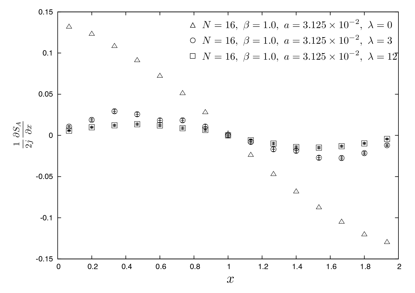

In this section, we study the interacting case. We perform Monte Carlo simulations at , and .
We again see a difference between odd and even , similar to the free case. We plot only the data for odd in the interacting case also.
In Fig. 7, we plot in the interacting case together with that in the free case against . We plot the data for (the interacting case) and for (the free case) after we subtract each value at from the data for each . We see that the shifted data are consistent with (3.5). This suggests that the finite temperature effect in is also proportional to the volume in the interacting case. The shape of the data in the interacting case is different from that in the free case, which should be attributed to non-locality of the interaction. Moreover, the magnitude in the interacting case is quite smaller than that in the free case.
As we stated in section 2.1, the length scale of nonlocality of the interaction is of order . Therefore we can, in general, expect that there is a transition from the “volume law” to the square of area law, where the “volume law” is given by the integral of the square of the area. We assume that the transition happens around . Namely, for EE behaves as the square of area law
| (5.1) |
which leads to
| (5.2) |
while for EE behaves as
| (5.3) |
which leads to
| (5.4) |
6 Conclusion and discussion
In this paper, we calculated EE in the scalar field theory on the fuzzy sphere using the method developed in [19]. In the free case, we confirmed that EE at zero temperature is proportional to the square of the area of the boundary and the leading contribution to it is proportional to the UV cutoff . We discussed the reason for this peculiar law. These behaviors are consistent with the observations in [8, 9]. We also found that the finite temperature effect in EE is proportional to the volume and independent of the UV cutoff . This property of the finite temperature effect is shared with ordinary local field theories.
In the interacting case, we performed Monte Carlo simulations to calculate EE. We found that the magnitude of EE in the interacting case is quite small compared to that in the free case. We observed a transition from the “volume law” to the square of area law for EE as the volume is increased. The former is obtained by integrating the latter over . This transition should originate from nonlocal nature of the interaction. We also found that the finite temperature effect in EE is proportional to the volume in the interacting case.
The fact that we can interpret our results geometrically following the division of the sphere in Fig.1(a) shows that the division of the matrix in Fig.1(b) works well.
In the interacting case, we need to study renormalization and the continuum limit. Indeed, at , , and , we obtained a good fit to the transition from the “volume law” to the square of area law for but not for . This suggests that the former is closer to the continuum limit than the latter.
In [9], it was shown that mutual information (MI) in the free case agrees with that in the ordinary scalar field theory on . This result is reasonable because MI is independent of the UV cutoff and the matrix model (2.3) with reduces to the ordinary scalar field theory on in the limit where the UV cutoff goes to infinity. We expect differences in the interacting case between MI in the noncommutative theory and that in the ordinary theory.
We hope to report progress in the above issues in the near future.
Acknowledgements
We would like to thank Shizuka Okuno for collaboration at an early stage of this work. Numerical computation was carried out on SR16000 and XC40 at YITP in Kyoto University and SR16000 and FX10 at the University of Tokyo. The work of A.T. is supported in part by Grant-in-Aid for Scientific Research (nos. 24540264, 23244057, and 15K05046) from JSPS.
References
- [1] S. Ryu and T. Takayanagi, Phys. Rev. Lett. 96, 181602 (2006) [hep-th/0603001].
- [2] A. Hashimoto and N. Itzhaki, Phys. Lett. B 465, 142 (1999) [hep-th/9907166].
- [3] J. M. Maldacena and J. G. Russo, JHEP 9909, 025 (1999) [hep-th/9908134].
- [4] W. Fischler, A. Kundu and S. Kundu, JHEP 1401, 137 (2014) [arXiv:1307.2932 [hep-th]].
- [5] J. L. Karczmarek and C. Rabideau, JHEP 1310, 078 (2013) [arXiv:1307.3517 [hep-th]].
- [6] S. Minwalla, M. Van Raamsdonk and N. Seiberg, JHEP 0002, 020 (2000) [hep-th/9912072].
- [7] N. Shiba and T. Takayanagi, JHEP 1402, 033 (2014) [arXiv:1311.1643 [hep-th]].
- [8] J. L. Karczmarek and P. Sabella-Garnier, JHEP 1403, 129 (2014) [arXiv:1310.8345 [hep-th]].
- [9] P. Sabella-Garnier, JHEP 1502, 063 (2015) [arXiv:1409.7069 [hep-th]].
- [10] D. Dou and B. Ydri, Phys. Rev. D 74, 044014 (2006) [gr-qc/0605003].
- [11] D. Dou, Mod. Phys. Lett. A 24, 2467 (2009) [arXiv:0903.3731 [gr-qc]].
- [12] S. Okuno, M. Suzuki and A. Tsuchiya, PTEP 2016, no. 2, 023B03 (2016) doi:10.1093/ptep/ptv192 [arXiv:1512.06484 [hep-th]].
- [13] T. Azuma, S. Bal, K. Nagao and J. Nishimura, JHEP 0405, 005 (2004) [hep-th/0401038].
- [14] T. Azuma, S. Bal and J. Nishimura, Phys. Rev. D 72, 066005 (2005) [hep-th/0504217].
- [15] J. Medina, W. Bietenholz, F. Hofheinz and D. O’Connor, PoS LAT 2005, 263 (2006) [hep-lat/0509162].
- [16] F. Garcia Flores, X. Martin and D. O’Connor, Int. J. Mod. Phys. A 24, 3917 (2009) [arXiv:0903.1986 [hep-lat]].
- [17] M. Panero, JHEP 0705, 082 (2007) [hep-th/0608202].
- [18] C. R. Das, S. Digal and T. R. Govindarajan, Mod. Phys. Lett. A 23, 1781 (2008) [arXiv:0706.0695 [hep-th]].
- [19] P. V. Buividovich and M. I. Polikarpov, Nucl. Phys. B 802, 458 (2008) [arXiv:0802.4247 [hep-lat]].
- [20] Y. Nakagawa, A. Nakamura, S. Motoki and V. I. Zakharov, PoS LATTICE 2010, 281 (2010) [arXiv:1104.1011 [hep-lat]].
- [21] E. Itou, K. Nagata, Y. Nakagawa, A. Nakamura and V. I. Zakharov, PTEP 2016, no. 6, 061B01 (2016) doi:10.1093/ptep/ptw050 [arXiv:1512.01334 [hep-th]].
- [22] C. S. Chu, J. Madore and H. Steinacker, JHEP 0108, 038 (2001) [hep-th/0106205].
- [23] P. Castro-Villarreal, R. Delgadillo-Blando and B. Ydri, Nucl. Phys. B 704, 111 (2005) [hep-th/0405201].
- [24] T. Banks, W. Fischler, S. H. Shenker and L. Susskind, Phys. Rev. D 55, 5112 (1997) [hep-th/9610043].
- [25] N. Ishibashi, H. Kawai, Y. Kitazawa and A. Tsuchiya, Nucl. Phys. B 498, 467 (1997) [hep-th/9612115].
- [26] R. Dijkgraaf, E. P. Verlinde and H. L. Verlinde, Nucl. Phys. B 500, 43 (1997) [hep-th/9703030].
- [27] J. P. Gazeau. Coherent states in quantum physics - 2009. Weinheim, Germany: WileyVCH.
- [28] G. Alexanian, A. Pinzul and A. Stern, Nucl. Phys. B 600, 531 (2001) [hep-th/0010187].
- [29] A. B. Hammou, M. Lagraa and M. M. Sheikh-Jabbari, Phys. Rev. D 66, 025025 (2002) [hep-th/0110291].
- [30] P. Presnajder, J. Math. Phys. 41, 2789 (2000) [hep-th/9912050].
- [31] G. Ishiki, Phys. Rev. D 92, no. 4, 046009 (2015) [arXiv:1503.01230 [hep-th]].
- [32] F. A. Berezin, Commun. Math. Phys. 40, 153 (1975).