Observational constraints on the generalized $\alpha$ attractor model

The past two decades of tremendous activities in observational cosmology motivated theorists to consider various theories of gravity. This leads to a plethora of cosmological models at the theoretical ground. The observations of Type Ia supernovae by the Supernova Cosmology Project and the High-Z Supernova Search Team provided strong evidence about the currently accelerated expansion of the Universe (against the presumed decelerating expansion caused by gravity). Baryon acoustic oscillations and results from the clustering of galaxies yielded more confirmatory evidences to this acceleration. Nowadays the concept of the late time cosmic acceleration has become a fundamental ingredient for theorists in modeling the Universe. The idea of the late time cosmic acceleration is mainly attributed to the presence of some mysterious entity commonly referred to as Dark Energy [1, 2, 3, 4, 5, 6, 7, 8]. Although there have been developed several ideas to explain the cosmic acceleration, the theory of Dark Energy is much more successful to explaining various phenomena. On the other hand, primordial inflation has taken a special status in explaining the origin of the anisotropies in the cosmic microwave background radiation (CMBR) and the formation of the large scale structure. The origin of both the early and late time inflation still represents a great theoretical puzzle which motivates theorists to invoke scalar fields to explain the two inflationary phases simultaneously. During the past three and half decades, a wide variety of inflationary models have been proposed, among which “cosmological attractors” was discovered very recently. These belong to a very broad class which incorporates the conformal attractors [9, 10], alpha attractors [11, 12, 13, 14, 15], and also includes scalar field cosmological models such as the Starobinsky model [16, 17, 18, 19, 20], the chaotic inflation in super-gravity (GL model) [21, 22, 23], Higgs inflation [24, 25, 26, 27, 28, 29, 30, 31, 32, 33] and axion monodromy inflation [34, 35, 36, 37, 38, 39, 40, 41]. All these have a mysterious fact in the context of recently released results obtained by WMAP and Planck data [42, 43, 44, 45] that they provide the very similar cosmological predictions, although they have different origins. For conformal attractors, they predict that, for a large number of $e$-folds $N$, the spectral index and tensor-to-scalar ratio are given by $n_{s}=1-2/N$ ; $r=12/N^{2}$. For $N\sim 60$, these predictions are $n_{s}\sim 0.967,r\sim 0.003$, while for $N\sim 50$, $n_{s}\sim 0.96,r\sim 0.005$, which are in very good agreement with WMAP and Planck data. For $\alpha$ attractors, the slow roll parameters $n_{s}$ and $r$ can be written as $n_{s}=1-2/N,r=12\alpha/N^{2}$ for small $\alpha$, and $n_{s}=1-2/N,r=12\alpha/(N(N+3\alpha/2))$ for large $\alpha$, where $N$ is the number of e-folds between the end of inflation and horizon-crossing, and its numerical value lies in the range $50\leq N\leq 60$. These models can be used not only for inflation but also for the late time cosmic acceleration [46, 47, 48, 49, 50, 51, 52, 53]. In this paper, we shall study the generalized $\alpha$ attractor model in the context of the late time cosmic acceleration.

The paper is organized as follows. In Section II, we present the basics of the $\alpha$ attractor models. Section III displays the evolution equations of the scalar field in the autonomous form and addresses the issue of the cosmological attractor. In Section IV, we use the joint data to carry out observational analyses and obtain constraints on the model parameters. Our results are summarized in Section V.

Here, we focus on the minimally coupled alpha attractors which are of more interest as they play an important role in cosmology to investigate the dark energy properties and to evaluate if these models can explain the late time cosmic acceleration. In the Einstein frame, the Lagrangian density of the alpha attractor model takes the form,

$$\mathcal{L}=\sqrt{-g}\left[\frac{1}{2}M_{p}^{2}R-\frac{\alpha}{\left(1-\frac{\varphi^{2}}{6}\right)^{2}}\frac{\left(\partial\varphi\right)^{2}}{2}-\alpha f^{2}\left(\frac{\varphi}{\sqrt{6}}\right)\right]$$

(1)

with a real scalar field $\varphi$. Despite of the changes in the inflaton potential and an arbitrary function $f\left(\varphi\right)$, this class of models has similar striking results for the primordial scalar perturbation tilt and tensor-to-scalar ratio. For $\alpha=1$, the Starobinsky model is recovered. We would like to note that the kinetic and potential energies have the same overall coefficient $\alpha$. The kinetic term is not canonical, but can be so through a field redefinition $\phi=\sqrt{6\alpha}\tanh^{-1}\left(\frac{\varphi}{\sqrt{6}}\right)$ with $V\left(\phi\right)=\alpha f^{2}\left(\tanh\left(\frac{\phi}{\sqrt{6\alpha}}\right)\right)$. We are interested in the dynamics of the scalar field and the evolution of its equation of state, and see whether it explains the late-time cosmic acceleration.

Two functional forms of $f$ have been employed for inflation,

	$\displaystyle f$	$\displaystyle=$	$\displaystyle c~\tanh\left(\frac{\phi}{\sqrt{6\alpha}}\right),$		(2)
	$\displaystyle\text{and}\qquad f$	$\displaystyle=$	$\displaystyle c~\frac{\tanh\left(\frac{\phi}{\sqrt{6\alpha}}\right)}{1+\tanh\left(\frac{\phi}{\sqrt{6\alpha}}\right)}$		(3)

The first one is known as the T model and the second one is the Starobinsky model ($\alpha$=1). Both models are identical at small $\phi$ and behave as the quadratic potential near the origin.

We consider a generalized $\alpha$ model given by [54]

$\displaystyle f$

$\displaystyle=$

$\displaystyle c~\frac{\tanh\left(\frac{\phi}{\sqrt{6\alpha}}\right)}{\left(1+\tanh\left(\frac{\phi}{\sqrt{6\alpha}}\right)\right)^{n}}$

(4)

where $c$ is a constant, $\alpha$ is a parameter, and $n$ is a number which can take the values $n=0,1,2,3,...$ Therefore, the potential of the generalized $\alpha$ model becomes

$\displaystyle V(\phi)$

$\displaystyle=$

$\displaystyle\alpha~c^{2}~\frac{\tanh\left(\frac{\phi}{\sqrt{6\alpha}}\right)^{2}}{\left(1+\tanh\left(\frac{\phi}{\sqrt{6\alpha}}\right)\right)^{2n}}$

(5)

As $\phi\rightarrow\infty$, the potential becomes constant (flatten), and as $\phi\rightarrow 0$, it behaves as a quadratic potential (see Figure 1).

Caldwell and Linder [55] revealed that the scalar field models can be divided into two categories: the fast roll (freezing) and slow roll (thawing) models. A freezing model is such that, during the matter/radiation era, the field mimics the background and remains sub-dominant. Only at late times, the field exits to late time cosmic acceleration. The freezing models remain independent for a wide range of initial conditions. This class corresponds to tracking freezing model. The another sub-class of freezing models is associated with the scaling solutions [56]. In this case, the energy density of the scalar field scales with the background energy density during most of the matter era.

In contrast, the thawing models are alike to inflaton that derives the acceleration of the Universe at early epoch. In the thawing models, the scalar field is initially frozen due to a large Hubble damping and behaves as a cosmological constant with $w\approx-1$. At late times the Hubble damping decreases and the scalar field slowly thaws from the frozen state and deviates from behavior of the cosmological constant. Thawing models are much sensitive to initial conditions. Some of the models of this class have been studied in [57, 58]. The thawing, tracker and scaling models have been discussed in [59].

The $\alpha$ attractor models seem to combine these two classes in one way. We consider the potential given by equation (5), which has the following asymptotic form

$\displaystyle\qquad V(\phi)\approx\alpha~c^{2}~2^{-2n}\left(1-2(2-n)e^{-\frac{2\phi}{\sqrt{6\alpha}}}\right),~~~~~~~~~~~~~~~~~~~\phi\gg\sqrt{\alpha}$

(6)

This is an uplifted exponential potential and studied as the inflationary models [21, 22, 23]. The exponential potential falls in the freezing class and approaches to a cosmological constant.

$\displaystyle\qquad\qquad V(\phi)\approx\frac{c^{2}}{6\alpha}\phi^{2},~~~~~~~~~~~~~~~~~~~~~~~~~~~~~\phi\ll\sqrt{\alpha}$

(7)

This is the quadratic potential, falls in the thawing class and deviates from the cosmological constant. The analytical solution of the average equation of state for the power-law potential $V(\phi)\propto\phi^{2p}$ is given by

$\displaystyle<w>$

$\displaystyle=$

$\displaystyle\frac{p-1}{p+1}$

(8)

For the quadratic potential $p=1$, therefore, in this case, as $\phi$ approaches to the origin, the time average equation of state during the oscillations is given by $<w>=0$.

The equations of motion are obtained by varying the Lagrangian density (1) with equation (5) have the following forms

$\displaystyle\frac{\dot{a}^{2}(t)}{a^{2}(t)}$

$\displaystyle=$

$\displaystyle\frac{1}{3M_{pl}^{2}}\left(\rho_{r}+\rho_{m}+\rho_{\phi}\right)$

(9)

$\displaystyle\ddot{\phi}+3\frac{\dot{a}}{a}\dot{\phi}+V^{\prime}(\phi)=0$

(10)

where a prime (^′) denotes the derivative with respect to $\phi$. In the following discussions we shall use the dimensionless variables

$$Y_{1}={\phi\over M_{p}},\quad Y_{2}={\dot{\phi}\over M_{p}H_{0}},\quad{\cal V}={V(Y_{1})\over M_{p}^{2}H_{0}^{2}}.$$

(11)

Using these new dimensionless variables, we can cast equations (9) and (10) as a system of the first-order equations

$$Y_{1}^{\prime}=\frac{Y_{2}}{h(Y_{1},Y_{2})}\,$$

(12)

$$Y_{2}^{\prime}=-3Y_{2}-{1\over h(Y_{1},Y_{2})}\Big[{d{\cal V}(Y_{1})\over dY_{1}}\Big]$$

(13)

The prime (^′) denotes the derivative with respect to $\ln(a)$, and the function $h(Y_{1},Y_{2})$ is given by,

$$h(Y_{1},Y_{2})=\sqrt{\left[{Y_{2}^{2}\over 6}+{{\cal V}(Y_{1})\over 3}+{\Omega_{0m}e^{-3a}}+{\Omega_{0r}e^{-4a}}\right]}$$

(14)

Here, $\Omega_{0r}$ and $\Omega_{0m}$ are the energy density parameters of radiation and matter, respectively at the present epoch. We solve the evolution equations (12) and (13) numerically, and the results are shown in Figures 1 - 4. Figure 1 exhibits the behavior of the potential (5) versus the scalar field $\phi$, in units of $c^{2}$ and Planck, respectively. The left panel is plotted for $n=0,1,2,3$. For large field values, the potential flattens to an uplifted plateau, while at small values it looks like the quadratic potential. The right panel is plotted for $n=0$ with various values of $\alpha$. The smaller values of $\alpha$ correspond to a more narrow minimum of the potential.

As the field evolving from the flatten region approaches the origin, the energy density $\rho_{\phi}$ undershoots the background and begins as thawing dark energy along with thawing behavior as the field freezes due to a large Hubble damping, and it lies in the thawing region even at the present epoch. However, in the future it switches over and converts to the scaling freezing behavior (see Figure 2).

The upper and lower right panels of Figure 2 show that the field oscillates most time between $w=\pm 1$, and correspondingly the average equation of state is $<w>=0$ at the attractor point (see Figure 3), which is consistent with the analytical result (8) for a quadratic potential.

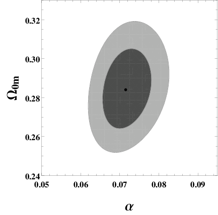
Figure 4 demonstrates the 1$\sigma$ (dark shaded) and 2$\sigma$ (light shaded) likelihood contours in the $\alpha-\Omega_{0m}$, $\alpha-c$ and $\Omega_{0m}-c$ planes with two different values of $n$, for the generalized $\alpha$ attractor model. The joint data (SN+Hubble+BAO+CMB) have been used to carry out the observational analysis. The best-fitting values of the model parameters for two distinct values of $n$ are shown in Table 1.

Our study shows that the $\alpha$ attractor model behaves as a $\phi^{2}$ potential when the scalar field approaches to origin. Before reaching the oscillatory phase, it has a slow-roll regime, which provides the late-time cosmic acceleration at the present epoch. Similar results can be obtained, if we use the $\phi^{2}$ potential rather than the $\alpha$ attractor. To confirm this, we consider the quadratic potential

$\displaystyle V(\phi)=V_{0}\left(\frac{\phi}{M_{p}}\right)^{2}$

(15)

We numerically evolve Eqs.(12) and (13) with (15). The results are presented in figure 5. The top and bottom left panels show the evolution of $\phi$, $\rho_{\phi}$ and $w$ versus the redshift. One can clearly see that before reaching the oscillatory phase, the field has a slow-roll regime, which gives the late-time cosmic acceleration at the current epoch. The bottom right panel exhibits the 1$\sigma$ (dark shaded) and 2$\sigma$ (light shaded) likelihood contours in the $V_{0}-\Omega_{0m}$ plane. The best-fit values of the model parameters are found to be $V_{0}=1.3534$ and $\Omega_{0m}=0.2846$. The best-fit values of $\Omega_{0m}$ for the quadratic potential and $\alpha$ model almost coincide, see Table 1. Therefore, both models provide a similar late-time cosmic acceleration at the present epoch, and are consistent with current observations.

We employ the $\chi^{2}$ analysis to constrain the model parameters. One can use the maximum likelihood method and get the total likelihood for the parameters $\alpha$, $\Omega_{0m}$ and $c$ as the product of individual likelihood for different datasets. The total likelihood function for joint data is given by

$$\mathcal{L}_{tot}(\alpha,\Omega_{0m},c)=e^{-\frac{\chi_{tot}^{2}(\alpha,\Omega_{0m},c)}{2}}$$

(16)

where

$\displaystyle\chi_{\rm tot}^{2}=\chi_{\rm SN}^{2}+\chi_{\rm Hub}^{2}+\chi_{\rm BAO}^{2}+\chi_{\rm CMB}^{2}\,,$

(17)

is related to Type Ia supernova (SN), data of Hubble parameter, Baryon Acoustic Oscillation (BAO) and Cosmic Microwave Background (CMB) data. The best fit value of the parameters is acquired by minimizing $\chi_{\rm tot}^{2}$ with respect to $\alpha$, $\Omega_{0m}$ and $c$. The likelihood contours in 1$\sigma$ and 2$\sigma$ confidence level are given as 2.3 and 6.17, respectively, in the two dimensional parametric space.

In this paper, we have investigated the generalized $\alpha$ attractor model that leads to the cosmological attractor behavior and can interpolate between the thawing and scaling freezing models. At the present epoch, it behaves as a thawing model whereas in the future it possesses scaling freezing behavior. In Figure 2, the dynamics of the scalar field and energy density $\rho_{\phi}$ are shown for $\alpha=0.05,0.1,1,10$. The evolution of $\rho_{\phi}$ starts off as a thawing dark energy along with thawing behavior, and even at the present epoch it lies in the thawing region. But in the future it switches over and turns to the scaling regime, which is cosmological attractor. For small values of the scalar field $\phi$, the generalized $\alpha$ attractor model mimics the power law behavior $V(\phi)\sim\phi^{2}$ and produces oscillations of $\phi$ near the origin which are reflected in the behavior of the equation of state $w$ (see Figure 2), and correspondingly the average equation of state parameter is $<w>=0$ (see Figure 3). In our setting, the scalar field remains in the slow roll regime but mimics the scaling behavior in the future. We considered two cases $n=1,2$, and used the joint data (SN+Hubble+BAO+CMB) to obtain the observational constraints on the model parameters. The best-fitting values of the model parameters for $n=1,2$ are $\alpha=0.0715$, $\Omega_{0m}=0.2841$ and $c=11.4884$, and $\alpha=0.0720$, $\Omega_{0m}=0.2849$ and $c=22.0320$, respectively.

We also considered the quadratic potential in order to compare with the results obtained from the $\alpha$ model. Figure 5 showed the evolution of $\phi$, $\rho_{\phi}$ and $w$ versus the redshift, and the 1$\sigma$ (dark shaded) and 2$\sigma$ (light shaded) likelihood contours in the $V_{0}-\Omega_{0m}$ plane. The best-fit values of the model parameters are found to be $V_{0}=1.3534$ and $\Omega_{0m}=0.2846$. The best-fit values of $\Omega_{0m}$ for both models are almost the same. Hence, in view of the current observations, both models are viable, and provide the late-time cosmic acceleration at the present epoch.

M.S. thanks M. Sami for making useful comments and suggestions. He is also thankful to M. Sajjad Athar for his constant encouragement throughout the work. A.W. is supported in part by NNSFC No.11375153 and No. 11675145, China.

References

- [1] E. J. Copeland, M. Sami, S. Tsujikawa, Int. J. Mod. Phys. D 15 (2006) 1753.
- [2] V. Sahni, A. A. Starobinsky, Int. J. Mod. Phys. D 9 (2000) 373.
- [3] M. Sami, New Adv. Phys. 10 (2016) 77-105.
- [4] M. Sami, R. Myrzakulov, Int. J. Mod. Phys. D 25 (2016) 1630031.
- [5] M. Sami, Curr. Sci. 97 (2009) 887.
- [6] M Sami, arXiv:0901.0756v1.
- [7] Md. Wali Hossain et al., Int. J. Mod. Phys. D 24 (2015) 1530014.
- [8] M. Sami, N. Dadhich, TSPU Vestnik 44N7 (2004) 25-36.
- [9] R. Kallosh and A. Linde, JCAP 07 (2013) 002.
- [10] R. Kallosh and A. Linde, JCAP 12 (2013) 006.
- [11] D. I. Kaiser and E. I. Sfakianakis, Phys. Rev. Lett. 112 (2014) 011302.
- [12] S. Ferrara, R. Kallosh, A. Linde and M. Porrati, Phys. Rev. D 88 (2013) 085038.
- [13] R. Kallosh, A. Linde and D. Roest, JHEP 11 (2013) 198.
- [14] R. Kallosh, A. Linde and D. Roest, JHEP 08 (2014) 052.
- [15] T. Miranda, J. C. Fabris and O. F. Piattella, JCAP 09 (2017) 041.
- [16] A. A. Starobinsky, Phys. Lett. B 91 (1980) 99.
- [17] V. F. Mukhanov and G. V. Chibisov, JETP Lett. 33 (1981) 532.
- [18] A. A. Starobinsky, Sov. Astron. Lett. 9 (1983) 302.
- [19] B. Whitt, Phys. Lett. B 145 (1984) 176.
- [20] L. A. Kofman, A. D. Linde and A. A. Starobinsky, Phys. Lett. B 157 (1985) 361.
- [21] A. S. Goncharov and A. D. Linde, Sov. Phys. JETP 59 (1984) 930.
- [22] A. B. Goncharov and A. D. Linde, Phys. Lett. B 139 (1984) 27.
- [23] A. Linde, JCAP 02 (2015) 030.
- [24] D. S. Salopek, J. R. Bond and J. M. Bardeen, Phys. Rev. D 40 (1989) 1753.
- [25] F. L. Bezrukov and M. Shaposhnikov, Phys. Lett. B 659 (2008) 703.
- [26] R. Fakir and W. G. Unruh, Phys. Rev. D 41 (1990) 1783.
- [27] D. I. Kaiser, Phys. Rev. D 52 (1995) 4295.
- [28] J. L. Cervantes-Cota and H. Dehnen, Nucl. Phys. B 442 (1995) 391.
- [29] E. Komatsu and T. Futamase, Phys. Rev. D 59 (1999) 064029.
- [30] S. Ferrara, R. Kallosh, A. Linde, A. Marrani and A. Van Proeyen, Phys. Rev. D 83 (2011) 025008.
- [31] S. Ferrara, R. Kallosh, A. Linde, A. Marrani and A. Van Proeyen, Phys. Rev. D 82 (2010) 045003.
- [32] A. Linde, M. Noorbala and A.Westphal, JCAP 03 (2011) 013.
- [33] R. Kallosh and A. Linde, JCAP 06 (2013) 027.
- [34] E. Silverstein and A. Westphal, Phys. Rev. D 78 (2008) 106003.
- [35] L. McAllister, E. Silverstein and A. Westphal, Phys. Rev. D 82 (2010) 046003.
- [36] J. P. Conlon, JCAP 01 (2012) 033.
- [37] R. Flauger, L. McAllister, E. Pajer, A. Westphal and G. Xu, JCAP 06 (2010) 009.
- [38] S. Hannestad, T. Haugbolle, P. R. Jarnhus and M. S. Sloth, JCAP 06 (2010) 001.
- [39] R. Flauger, L. McAllister, E. Silverstein, A. Westphal, arXiv:1412.1814.
- [40] T.C. Bachlechner, C. Long, and L. McAllister, JHEP 01 (2016) 091.
- [41] J. Brown, W. Cottrell, G. Shiu, and P. Soler, arXiv:1607.00037.
- [42] Planck Collab. (P. A. R. Ade et al., Astron. Astrophys. 571 (2014) A22.
- [43] Planck Collab. (P. A. R. Ade et al., A & A 571 (2014) A16.
- [44] Planck Collab. (P. A. R. Ade et al., arXiv:1502.02114 [astro-ph.CO].
- [45] Planck Collab. (P. A. R. Ade et al., A & A 594 (2016) A13.
- [46] S. Ferrara, R. Kallosh and A. Linde, JHEP 10 (2014) 143.
- [47] I. Antoniadis, E. Dudas, S. Ferrara and A. Sagnotti, Phys. Lett. B 733 (2014) 32.
- [48] R. Kallosh and A. Linde, JCAP 01 (2015) 025.
- [49] G. Dall’Agata and F. Zwirner, JHEP 12 (2014) 172.
- [50] R. Kallosh, A. Linde and M. Scalisi, JHEP 03 (2015) 111.
- [51] A. B. Lahanas and K. Tamvakis, Phys. Rev. D 91 (2015) 085001.
- [52] R. Kallosh and A. Linde, Phys. Rev. D 91 (2015) 083528.
- [53] J. J. M. Carrasco, R. Kallosh and A. Linde, JHEP 10 (2015) 147.
- [54] E. V. Linder, Phys. Rev. D 91 (2015) 123012.
- [55] R. R. Caldwell and E. V. Linder, Phys. Rev. Lett. 95 (2005) 141301.
- [56] E. J. Copeland, A. R. Liddle, and D. Wands, Phys. Rev. D 57 (1998) 4686.
- [57] M. Shahalam, S. Sami, A. Agarwal, Mon. Not. R. Astron. Soc. 448 (2015) 29482959.
- [58] R. Myrzakulov and M. Shahalam, Gen. Rel. Grav. 47 (2015) 81.
- [59] T. Chiba, A. D. Felice and S. Tsujikawa, Phys. Rev. D 87 (2013) 083505.
- [60] N. Suzuki, D. Rubin, C. Lidman, G. Aldering, R. Amanullah, K. Barbary, L. F. Barrientos and J. Botyanszki et al., Astrophys. J. 746 (2012) 85.
- [61] R. Lazkoz, S. Nesseris, L. Perivolaropoulos, J. Cosmol. Astropart. Phys. bf11 (2005) 010.
- [62] O. Farooq and B. Ratra, Astrophys. J. 766 (2013) L7.
- [63] C. Zhang, H. Zhang, S. Yuan, T. -J. Zhang and Y. -C. Sun, arXiv:1207.4541 [astro-ph.CO].
- [64] J. Simon, L. Verde and R. Jimenez, Phys. Rev. D 71 (2005) 123001.
- [65] M. Moresco, L. Verde, L. Pozzetti, R. Jimenez and A. Cimatti, JCAP 07 (2012) 053.
- [66] C. -H. Chuang and Y. Wang, arXiv:1209.0210 [astro-ph.CO].
- [67] C. Blake, S. Brough, M. Colless, C. Contreras, W. Couch, S. Croom, D. Croton and T. Davis et al., Mon. Not. Roy. Astron. Soc. 425 (2012) 405.
- [68] D. Stern, R. Jimenez, L. Verde, M. Kamionkowski and S. A. Stanford, JCAP 1002 (2010) 008.
- [69] N. G. Busca, T. Delubac, J. Rich, S. Bailey, A. Font-Ribera, D. Kirkby, J. M. Le Goff and M. M. Pieri et al., Astron. Astrophys. 552 (2013) A96.
- [70] C. Blake, E. Kazin, F. Beutler, T. Davis, D. Parkinson, S. Brough, M. Colless and C. Contreras et al., Mon. Not. Roy. Astron. Soc. 418 (2011) 1707.
- [71] SDSS Collab. (W. J. Percival et al.), Mon. Not. Roy. Astron. Soc. 401 (2010) 2148.
- [72] F. Beutler, C. Blake, M. Colless, D. H. Jones, L. Staveley-Smith, L. Campbell, Q. Parker and W. Saunders et al., Mon. Not. Roy. Astron. Soc. 416 (2011) 3017.
- [73] N. Jarosik, C. L. Bennett, J. Dunkley, B. Gold, M. R. Greason, M. Halpern, R. S. Hill and G. Hinshaw et al., Astrophys. J. Suppl. 192 (2011) 14.
- [74] D. J. Eisenstein et al. [SDSS Collaboration], Astrophys. J. 633 (2005) 560.
- [75] R. Giostri, M. V. d. Santos, I. Waga, R. R. R. Reis, M. O. Calvao and B. L. Lago, JCAP 1203 (2012) 027.
- [76] E. Komatsu et al., ApJS 192 (2011) 18.
- [77] W. Hu and N. Sugiyama, Astrophys. J 471 (1996) 30.