Exponential Networks and Representations of Quivers
| Richard Eager†, Sam Alexandre Selmani†‡ and Johannes Walcher† |
| † Mathematical Institute, |
| Heidelberg University, Heidelberg, Germany |
| ‡ Department of Physics, |
| McGill University, Montréal, Québec, Canada |
Abstract
We study the geometric description of BPS states in supersymmetric theories with eight supercharges in terms of geodesic networks on suitable spectral curves. We lift and extend several constructions of Gaiotto-Moore-Neitzke from gauge theory to local Calabi-Yau threefolds and related models. The differential is multi-valued on the covering curve and features a new type of logarithmic singularity in order to account for D0-branes and non-compact D4-branes, respectively. We describe local rules for the three-way junctions of BPS trajectories relative to a particular framing of the curve. We reproduce BPS quivers of local geometries and illustrate the wall-crossing of finite-mass bound states in several new examples. We describe first steps toward understanding the spectrum of framed BPS states in terms of such “exponential networks.”
November 2016
eager@mathi.uni-heidelberg.de, sam.selmani@physics.mcgill.ca, walcher@uni-heidelberg.de
It is a capital mistake to theorize before you have all the evidence. It biases the judgment. (Sherlock Holmes)
1 Introduction
The spectrum of BPS states plays a prominent role in the study of quantum mechanical theories with extended supersymmetry and in the interest of such theories for mathematics. Of particular significance are theories with eight real supercharges, such as four-dimensional gauge theories with supersymmetry, or compactifications of M-theory or type II string theory on Calabi-Yau threefolds.
In such models, the intrinsic representation data of the supersymmetry algebra (BPS charges and masses, their monodromy and singularities, the chiral metric) fit together in such a tightly constrained way over the moduli space of vacua that its geometric structure can be recovered from a clever combination of local flatness and global consistency conditions. Typically, this data can be solved for by studying the classical variation of an auxiliary spectral geometry. For string/M-theory, this is the Calabi-Yau manifold itself (or rather, its mirror), and for gauge theory, Seiberg-Witten geometry. These connections are extremely well understood, admit generalizations to gravitational and higher-derivative corrections of the effective theory, and include relations to classical and quantum integrable systems and a variety of interesting mathematics.
On the other hand, determining the representation content, i.e., describing the actual BPS subspace of the Hilbert space, is much more subtle, and it is not in general clear to what extent this data is determined by the properties of the vacuum manifold alone. This has to do with the fact that while the graded dimensions of the space of BPS states (the BPS degeneracies) are locally constant over the moduli space, they can jump discontinuously at the crossing of certain real co-dimension-one walls. There is by now a lot of circumstantial evidence that wall-crossing is not incompatible with the idea that the BPS spectrum is in fact determined by the effective low-energy dynamics. First of all, the location of the walls of course follows from the properties of the charge lattice (the central charge), which is determined by special geometry. Secondly, the change of the BPS spectrum across the walls can be studied from the dynamics of bound states in the effective theory [1] and is subject to the fully general formula of Kontsevich-Soibelman [2]. The first physics derivation of this Kontsevich-Soibelman wall-crossing formula [3] exploits precisely the tension between the discontinuous changes in the BPS degeneracies and the smoothness of the hyperkähler metric to which they contribute. In special cases, these constraints allow for a full calculation of the BPS spectrum [4, 5]. Moreover, at least for strings on Calabi-Yau, the OSV conjecture [6] offers an even more general relation between the BPS degeneracy and the topological (string) partition function whose asymptotic expansion captures the perturbative corrections to the low-energy theory.
With or without assuming that these intricate consistency conditions can ultimately be completely solved, it is fruitful to also investigate the BPS spectrum more directly from the point of view of the spectral geometry. In string compactifications, for instance, BPS states arise by wrapping D-branes on supersymmetric cycles in the Calabi-Yau, and their degeneracies are encoded in the cohomology of the associated moduli spaces. It is then not only satisfying to identify precisely the problem to which the wall-crossing formulas provide an answer, but the explicit solution to some subclass also provides valuable complementary information to check the various conjectures.
The present paper grew out of attempts to generalize the geometric description of BPS states in four-dimensional supersymmetric gauge theories that was given by Klemm-Lerche-Mayr-Vafa-Warner [7]11 1 See citations of [7] for other work done in the 1990’s. and that has received renewed interest in recent years following the work of Gaiotto-Moore-Neitzke on spectral networks [5]. This approach, which we will review below, can be seen to arise in a suitable limit from the geometric realization of the gauge theories, either by 2-branes ending on 5-branes in M-theory, or by dimensional reduction of 3-branes wrapping supersymmetric cycles in type IIB string theory.
The main idea and motivation for the generalization we are seeking can be explained from that second point view: The type IIB local geometries are the mirror manifolds of the toric Calabi-Yau manifolds that geometrically engineer the gauge theory in type IIA. In this context, it is known that the 3-fold geometry reduces to an effective one-dimensional description even before taking the gauge theory limit to the Seiberg-Witten curve, and that this holds also for local toric geometries that do not admit a gauge theory interpretation. Among the evidence for this statement we mention the coincidence of the period calculation [8, 9], the evaluation of D-brane probes [10], the so-called remodeling conjecture [11], as well as modularity in its various forms. Our work will provide additional corroboration.
In the A-model, BPS states arise from B-branes. Their counting is, in many instances, rather well understood mathematically in terms of the cohomology of moduli of coherent sheaves, and many of the conjectures that we alluded to above have been checked and verified. It is known in principle that the problem whose solution reproduces the BPS state counting in the B-model is related to the moduli of special Lagrangian submanifolds (stable A-branes). Making this explicit is, however, complicated by the need to complexify the moduli space to resolve certain uncontrolled singularities, and by the obstructions by holomorphic disks whose effects on the problem are still not completely understood.
We will not be able to fully fill this important gap in this paper. However, we will give, in some simple examples, a proof of principle that BPS degeneracies in local Calabi-Yau manifolds can be understood from the B-model perspective in terms of a calibrated geometry that is the reduction of special Lagrangian geometry to the mirror curve, suitably corrected by holomorphic disks.
To this end, we will study the analogue of spectral networks in the simplest possible examples of local Calabi-Yau manifolds. We will attempt to reproduce as much as possible of the BPS spectrum that is known from the A-model for these geometries. A useful tool that is shared by the A- and B-model is the description of D-brane bound states in terms of the representation theory of so-called BPS quivers [12, 13, 14]. This theory also plays an important role in our story.
An interesting payoff of our work is a kind of “reversed” perspective on mirror symmetry à la Strominger-Yau-Zaslow for local Calabi-Yau manifolds. Recall that in the SYZ picture, the mirror manifold is interpreted as the moduli space of a particular special Lagrangian 3-torus. This picture is in principle completely symmetric between A- and B-model for any given mirror pair. In the local case, however, one usually starts from A-branes on the toric side, and reconstructs the mirror as a Landau-Ginzburg model from the obstruction theory of the toric fibers. In our examples, we will start from a particular calibrated submanifold in the B-model (as we will see, a suitable spectral network), whose moduli space is related (after complexification) to the original toric manifold.
The paper is organized as follows. We begin in section 2 with a brief review of the work that we will generalize, and a summary of the new features that derive from the exponential nature of the differential on the local mirror curves. We give further mathematical details in section 3, and an overview of the current state of our theory in section 4. In our first example, section 5, we reproduce the finite BPS spectrum of the conifold by exploiting a new junction rule for BPS trajectories. The main feature appears in section 6, in which we produce exponential networks for a large class of BPS states on local . We concentrate on states with a reasonable quiver representation, and study their wall-crossing under variation of the stability condition. In section 7, we return to what should be regarded as the simplest example of a Calabi-Yau, , and describe our best attempts at framed BPS states in this model. Along the way, we study the moduli space of a distinguished state that is mirror to a single pure D0-brane (a calibrated version of what is known in symplectic geometry as the “Seidel Lagrangian” [15, 16]), and show that this moduli space retracts to the toric diagram of the A-model Calabi-Yau.
2 BPS Trajectories, Quivers, and Mirror Symmetry
The main goal of this paper is to provide a new, B-model, perspective on BPS
states of local Calabi-Yau manifolds by combining and generalizing the following
lines of research:
(i) The description of BPS states in four-dimensional supersymmetric
gauge theories (of “class ”) in terms of spectral networks on
Riemann surfaces given by Gaiotto-Moore-Neitzke [5], and follow-up
work.
(ii) Local mirror symmetry as consolidated by Hori-Vafa [9], which
identifies the mirror of local toric Calabi-Yau manifolds with conic
bundles over degenerating over a Riemann surface
called the mirror curve.
(iii) The wealth of knowledge about BPS states in these models that has
accumulated over the past fifteen years. We will rely in particular on the relation
to the representation theory of suitable BPS quivers, which in the case of
(“complete”) gauge theories has been related to the
spectral curve perspective by Alim et al. [14].
We begin with brief reviews of each of these topics.
2.1 Spectral networks
The solution of supersymmetric gauge theories in four dimensions in terms of a suitable “spectral” (Seiberg-Witten) curve includes a fruitful representation of their spectrum of massive BPS states. The basic idea is to embed the gauge theory in a higher-dimensional setup where the spectral geometry becomes part of the space-time, and BPS particles in four dimensions are realized geometrically as extended objects calibrated by the Seiberg-Witten differential. This approach was pioneered in [7] and championed by [5]. For more on the early development of the subject see the review [17] and references therein.
Theories of class
The large class of such theories studied in [5] are defined as the result of dimensional reduction (with a partial topological twist) of the six-dimensional theories associated to an ADE Lie algebra on a punctured Riemann surface with certain defect data at the punctures. In the embedding in M-theory, the theories arise on the world-volume of M5-branes wrapped on . At a generic point on the Coulomb branch, the IR description involves a single M5-brane wrapped on , where is the spectral cover
| (2.1) |
and is a -valued 1-form on that parametrizes the moduli space of vacua. For convenience, we will take in what follows.
The six-dimensional theory contains string-like excitations that arise as boundaries of M2-branes ending on the stack of M5-branes. When extended along paths of , these strings give rise to particles upon dimensional reduction to four dimensions. For states of finite mass, the M2-brane should have finite spatial volume. This means that with respect to a local trivialization of the spectral cover, the paths are labelled locally by a pair of integers . Such a string is locally BPS if it saturates the condition
| (2.2) |
where and is the restriction of the Liouville 1-form on to the th sheet. This condition is satisfied if and only if for some phase and some orientation of the path. (Equivalently, the condition is that , and we use as volume form.) Following [5], we call such a locally minimizing path an trajectory of phase .
The spectral network is simply the “life story” of such BPS trajectories drawn on the Riemann surface . To describe it, we assume for simplicity that all branch points of the covering (2.1) are simple. Then, from an branch point of the spectral cover emanate three trajectories for any phase . This can be seen by writing and noting that
| (2.3) |
has three independent solutions . Also note that depending on the placement of the branch cut, two of these trajectories are of type , and one is of type . As the trajectories emanating from the various branch points evolve around , it is possible that they meet. The pronouncement is that when an - and -trajectory meet, an -trajectory is born, as illustrated in Figure 2. The collection of all trajectories emerging from the branch points and born in collisions is called the spectral network of phase .
Generically, the trajectories will eventually be attracted to one of the punctures of and crash. At special values of , however, it may happen that some of the BPS trajectories terminate at a branch point or collide head-on. This gives rise to a closed subset of the plane with the geometry of a trivalent graph of finite total length that we call a “finite web” following [5] (see Figure 4 for relevant examples). A finite web corresponds to a state of a finite mass BPS particle in four dimensions. Under the identification of the lattice of electric-magnetic charges of the 4d theory with , the charge of a finite web is the homology class of its canonical lift to determined by the labelling on the strands. The Dirac-Schwinger-Zwanziger pairing between electric and magnetic charges is identified with the intersection pairing on homology. In the M-theory picture, the BPS particles arise from M2-branes ending on the M5 branes, connecting the two lifts pointwise along the finite web. The BPS nature of the junction can be verified in this setup, see e.g. [18].
To determine BPS degeneracies from the counting of finite webs with fixed charge, one has to take into account that finite webs might exist in continuous families, of which the spectral network only produces some “critical members” (as is the case for example in Figure 4(d)), whereas the generic member does not pass through the branch points, but is still locally calibrated and satisfies the junction rules. These deformations of the finite webs realize geometrically the zero modes of BPS particles in 4d. In such a situation, the BPS degeneracies should be determined by quantizing those zero modes. It appears, however, that the information about the degeneracies can in fact be read off purely from the critical pictures that arise from the spectral network without deformations. The prescription of [5] for calculating these degeneracies results from considering not only BPS particles but also line and surface defects, and thoroughly analyzing the consistency of the wall-crossing behavior of particles bound to them. Indeed, the curve is identified as the parameter space of UV couplings of a canonical surface defect and finite webs with an open end at the point are identified as a particle bound to the surface defect . Line defects, which can be thought of as infinitely heavy particles arising from M2 branes stretching infinitely in one cotangent direction, are represented by the (uncalibrated) homotopy class of a path on .
In this paper we supply evidence that a similar story holds for BPS degeneracies of D-branes in toric Calabi-Yau 3-folds. In these models, it is natural to propose that the finite webs arising from the network should be viewed as the fixed points of the given torus action on the associated D-brane moduli spaces. We have not yet fully fleshed out this correspondence, but we expect that a generalization of the analysis of [5] including line and surface defects will lead directly to a complete and systematic algorithm for determining BPS degeneracies in these models as well [19].
A useful heuristics: D-branes on the torus
One of the premises of our analysis is the relation between the combinatorics of spectral networks and their geometric deformations on the one hand, and the dynamics of the associated BPS states on the other. For an example of this, consider a D2-brane wrapping a torus, with a D0-brane sitting somewhere on it. Condensation of the open string tachyon in this system corresponds to dissolving the D0-brane into flux. This can be seen more graphically in the T-dual picture, in which the D2 and D0-branes become a pair of perpendicular D-branes. The tachyonic D-D’-string is localized at their intersection and its condensation corresponds to resolving the intersection, resulting in a D-brane at an angle (if we must, call it a simple “network” of D branes). Upon T-duality in the same direction as the first, the result is mapped back to a D2 brane with magnetic flux on it.

This would essentially be the story of “spectral networks and mirror symmetry for Calabi-Yau 1-folds”. We will also find useful the heuristic interpretation of resolving intersections as condensing tachyonic fields, especially in relation to the quiver description.
The pure theory
| Weak Coupling | Strong Coupling |
|---|---|
| Dyons | Dyon |
| W-boson | Monopole |
For another illustrative example, consider the original “pure glue” Seiberg-Witten theory [20]. The charge lattice is just , with basis and . The moduli space of vacua is the complex -plane, with singular locus dominated by the lightest particles of charge , and respectively. In the weak coupling regime (large ), there is an infinite number of stable BPS particles with charges , as well as the bosons with charges . Famously, there is a (topologically circular) line of marginal stability passing through and , on the other side of which the stable spectrum consists of only the monopole of charge and dyon of charge . The central charge of a BPS particle with charge is given by where , are certain hypergeometric functions, arising as periods of the elliptic curve 2.4. The monopole and dyon are naturally thought of as the basic states of which the others are bound states. To simplify the exposition in the rest of the paper we represent the charge of the monopole as and the charge of the dyon as In terms of the previous electric-magnetic charge basis, .
The geometric realization is as follows. The spectral curve is a genus 1 double cover with two punctures and two simple ramification points:
| (2.4) |
With two branches, there is only one type of strand on , so junctions do not occur. There are two “elementary” finite webs shown in Figures 4(a)-4(b). These are identified (up to monodromy) via their central charge with the monopole and the dyon, which exist at any . At large , there is an infinite family of “spirals” formed by concatenating copies of one of the elementary webs with copies of the other, separating them from the branch points and straightening them out in the process. These have electric-magnetic charge and , respectively.
There are also bound states of one copy of each of the two basic states that are realized by closed loops. The closed loops actually exist in a family interpolating between the two loops attached at either branch point. The Hilbert space of 1-particle states associated to this family of loops is in principle the cohomology of its moduli space. The algorithm of Gaiotto-Moore-Neitzke [5] gives the invariant trace over this Hilbert space as , reflecting the contribution of a BPS vector multiplet.
Note that the existence of the bound states depends geometrically on the ability to locally shorten the web by detaching the strands from the branch point, because the angle between the two elementary webs is less that . In the strong coupling regime, this is no longer possible, and all bound states cease to exist.
2.2 Mirror curves for toric Calabi-Yau manifolds
It is well known that the embedding of gauge theories of class into M-theory by wrapping M5-branes on punctured Riemann surfaces is related, by a sequence of dualities, to geometric engineering of gauge theories in type II string theory. In this approach, the gauge dynamics arises from D-branes wrapping vanishing cycles in local singularities of Calabi-Yau manifolds. One typically starts in type IIA (where computations are done in the “A-model”) with a toric Calabi-Yau threefold, , which is equivalent by mirror symmetry to type IIB (the “B-model”) on a Calabi-Yau of the form
| (2.5) |
Here, is a certain Laurent polynomial determined by the toric data. For a suitable design, the curve (2.1) arises in a scaling limit from the mirror curve which is the locus where the conic fibration degenerates. It is in fact in this context that the description of BPS states in terms of “geodesics on the Seiberg-Witten curve” was originally derived in [7]. We review the setup here in order to emphasize the points in which the full result departs from the gauge theory limit. We start in the A-model with the gauged linear sigma model (GLSM) description of the toric threefold.
Local mirror symmetry
We let be the “rank” of the Abelian gauge group , and the charges of the chiral fields. We assume that these charges satisfy the Calabi-Yau condition
| (2.6) |
and denote the Fayet-Iliopoulos couplings by for each . The toric manifold then arises as the solution of the D-term constraints
| (2.7) |
on the lowest components of the chiral fields, taken modulo gauge equivalence. The space can be described more mathematically as the symplectic reduction or GIT quotient with stability specified by the , which become (the real part of) the Kähler parameters of . In the process, the become homogeneous coordinates on .
In [9], Hori and Vafa derived the theory mirror to by applying T-duality to the argument of all the chiral fields in the GLSM. They showed that in terms of the variables
| (2.8) |
the mirror of the GLSM is the Landau-Ginzburg theory with superpotential
| (2.9) |
on the solution of a complexification of (2.7),
| (2.10) |
where are the exponentiated and complexified Kähler parameters.
By now, mirror symmetry between and this Landau-Ginzburg model has been checked in great detail, and the equivalence of the topological models has the status of a mathematical theorem. Ultimately, the duality of course also holds at the level of the full physical theory, including the BPS spectrum in space-time. The resulting mathematical statements are however more difficult to check directly, mostly because stability of D-branes in Landau-Ginzburg models still is only partially understood [21].
In this paper, we will use the relationship between the Landau-Ginzburg model (2.9) and the Calabi-Yau hypersurface (2.5) in the form in which local mirror symmetry was initially discovered. While this reduction is slightly less than fully rigorous at this point (although its validity at the topological level is beyond doubt), it puts us in a position to perform some explicit checks of the BPS spectrum. The easiest way to see the relation is to consider the evaluation of the periods: The statement that the fundamental variables are means that the holomorphic volume form is the residue of
| (2.11) |
on the solutions of (2.10). Solving these equations in terms of three of the variables, , , , and factoring out one of them by homogeneity, we define by the equation
| (2.12) |
For a contour along which the integral converges, we can insert a Gaussian to rewrite the periods of (2.11) as
| (2.13) |
where the last step is the Griffiths-Poincaré residue that gives us the standard form of the holomorphic three-form on the hypersurface (2.5).
Granting (2.5), the study of supersymmetric A-branes in can be further reduced to the “mirror curve”
| (2.14) |
endowed with the differential
| (2.15) |
by “integrating over the fibers” of the map sending to [7]. Over each point in the -plane the equation , viewed as an equation on , describes an affine conic that is reducible precisely when . The generic conic has the topology of a cylinder , and a “minimal” given by the intersection of with , in other words . This shrinks to a point precisely on the curve , so that tracing the along any path in -space that intersects precisely at the beginning and end of the path gives rise to a two-sphere . Assuming that the path begins and ends at the same value of , but at possibly different values of and , we can evaluate the integral
| (2.16) |
which gives the differential (2.15) up to factors of . We’ll work in the normalization (2.15) in the following.
Initial observations
Note that in (2.16) we have to allow and to stand for different branches of the logarithm if the path winds around the origin in the -plane. More formally, the mirror curve description of toric Calabi-Yau threefolds is an instance of a branched covering embedded in , where is the zero-section, with a holomorphic symplectic form that in a local coordinate on takes the form . In contrast to the ordinary spectral cover (2.1), this form is not exact, although the exponential of the local “Liouville form” is still single-valued. We emphasize that it would be a mistake to replace by an infinite covering on which is well-defined – only the winding number in the fiber direction is detected by (2.16), and not the absolute choice of branch itself.
As far as we know, the geometry associated with such “exponential differentials” has not been studied in the literature so far, although the problems arising from the winding in the fiber direction were mentioned back in [22]. We note however, that these multi-valued differentials play a central role in what is known as the “remodeling” description of the topological string on local Calabi-Yau manifolds [23]. In this approach, the formalism of topological recursions developed by Eynard-Orantin [24] is lifted to curves in , with appropriate modifications of the local residue calculus at the branch points. Given the striking similarities with the gauge theory setup, it is very natural to expect that “exponential” versions of spectral networks will capture the BPS spectrum in the same fashion.
Another way to understand the close analogy between mirror curves (2.5) and the spectral curves for gauge theories (2.1) is through the interpretation of these curves as “IR moduli spaces” of defects of the respective theories. This interpretation gives an alternative derivation of the differential (2.15) by reduction along the non-compact cycles instead of the compact cycles in the fibers of (2.5). Following the original approach of Aganagic and Vafa [10], consider a probe brane given by one of the two components, say of the singular fiber over some given point of the mirror curve. Even though such a brane is holomorphic for any point on the curve, a non-trivial superpotential arises on account of the non-compactness of the cycle on which the brane is wrapped. We fix one of coordinates, say , at infinity on the brane world-volume, which is identified with the -plane. The other coordinate, say , is treated as a holomorphic modulus. Then, the superpotential is calculated as a chain integral over the three-chain of the form
| (2.17) |
with , and functions , subject to the conditions
| (2.18) |
With these conditions, and assuming a radially symmetric profile for for simplicity, one easily finds [10]
| (2.19) |
where the last integral is a contour integral on , as claimed.
Framing
An important aspect of this derivation is the dependence of the differential on the mirror curve on the brane that is used as a probe, a degree of freedom known as “framing” [25]. In the A-model, the toric brane (of topology ) that is mirror to the fibers is specified by a point on the toric diagram (the projection of a one-dimensional linear subspace of the base of the toric fibration). The vertex of the toric diagram closest to that point is surrounded by three faces, corresponding to toric divisors say , , as in Fig. 5. Then, modulo the D-term equations (2.7), the brane is specified by
| (2.20) |
and the modulus is . The semi-classical regime is when the brane is far from the vertex (which requires in particular, if the brane sits on an internal leg, that leg to be long). In the quantum regime, captured by the mirror, (2.20) ceases to vanish, and the modulus is subject to the framing ambiguity
| (2.21) |
(Note that disappears under (2.20)!) In other words, the good variables to use in (2.12) are and which are defined by
| (2.22) |
and in these variables the differential on is given by (2.15). Alternatively, we may also use , with necessary changes.
The idea of the spectral network approach to BPS states is that open webs capture the degeneracy of solitons bound to defects represented by their endpoints, whereas closed finite webs correspond to the “vanilla”, or purely 4d, BPS particles. As a result, the degeneracy of the finite webs that we construct from our exponential networks should be independent of the framing, even though the respective differentials might differ by exact terms. This framing independence provides an important check on our formalism.
2.3 BPS Quivers
The third starting point of our investigation is the description of BPS spectra in terms of quivers, which also has a long history going back to [26] in the physics literature and builds on earlier mathematical work by Nakajima, Kronheimer, and ultimately Gabriel and Kac [27, 28, 29, 30]. The basic physical idea is to study BPS states and their interactions from the point of view of the effective theory on their world-volume (supersymmetric quantum mechanics in the case of BPS particles). This point of view is particularly convenient to understand the formation of bound states in terms of “tachyon condensation” in the effective theory and the decay into constituents in terms of Higgs-Coulomb transitions induced by the variation of couplings in the background space-time theory.
The quiver description arises when, under certain conditions, it is possible to build up the entire spectrum of BPS states by bound state formation out of a finite number of “basic states”. These basic states, which as a minimum requirement must generate the BPS charge lattice of the theory under consideration, form the nodes of the quiver diagram. The gauge group of the world-volume theory on some integral combination of the basis states is a product over the nodes of the given rank. The chiral fields in bifundamental representations that allow the formation of bound states form the arrows of the quiver. The gauge-invariant superpotential is a formal sum of traces over closed loops in the quiver, and the D-terms depend on Fayet-Iliopoulos parameters associated with the factors at each node. The supersymmetric vacua correspond to stable representations of the quiver algebra [31].
Mathematical recapitulation
To explain this identification and establish some notation, we state that our
quiver is specified by a tuple , where the finite sets and collect the nodes
and arrows, respectively, and the maps and specify the head and
tail of an arrow. Given this, a representation of is specified by
[32]
A finite-dimensional vector space for each node in
.
A -linear map
for each arrow in
For any representation of , the assignment of the dimension
of to each vertex is called the dimension vector
of . Given an ordering of the vertices of , the
dimension vector has components , but we will often denote it simply by .
Given two representations and of a quiver a morphism of quiver representations is a family of linear maps
| (2.23) |
such that The category of representations of a quiver is equivalent to the category of modules over the path algebra In particular is a category with kernels and cokernels. A representation over a quiver is a subrepresentation of a representation if there is an injective morphism More concretely, this means that and the homomorphisms are induced from the restriction of homomorphisms
As a simple example, consider the generic representations
| (2.24) |
of the Kronecker-2 quiver from Fig. 6 with dimension vector . For or there are no sub-representations with dimension vector since it is impossible for the square
| (2.25) |
to be commutative. However there are sub-representations with dimension vector which we will consider shortly.
A representation is called indecomposable if it cannot be expressed as the direct sum of two non-zero representations. For example, for any , the representation
| (2.26) |
of the Kronecker-2 quiver is indecomposable [33]. It is however not irreducible in the familiar sense of representation theory, since it admits (2.24) with as a non-trivial sub-representation in an obvious way.
The complex algebraic group acts on the space of quiver representations of fixed dimension vector. It appears physically as the complexification of the gauge group of the effective world-volume theory. In this theory, (classical) supersymmetric vacua correspond to solutions of the D-term constraints22 2 In the presence of a superpotential, the relevant representations are those of the quiver path algebra with relations. This plays a role in our examples later, but for now, we assume that the F-term constraints have been solved. modulo the action of . Equivalently, one may consider the space of those orbits that contain a solution of the D-terms. In other words, on each orbit the solution of the D-terms (if one exists) is unique up to the action of . Mathematically, this is the correspondence between the symplectic and algebraic quotient constructions of moduli spaces, which was established for quiver representations by King [34]. In this context, the “good” orbits are those that are “stable”, in the sense of Mumford’s numerical criterion, with respect to a character of that is related physically to the FI-parameters entering the D-term constraints.
More concretely, a King stability condition for quiver representations is specified by a map . An indecomposable representation of is -semistable if
| (2.27) |
and for every sub-representation of ,
| (2.28) |
The representation is -stable if additionally the only sub-representations with are and . As an example, we again consider the representations of the Kronecker-2 quiver with dimension vector . As we have seen, the generic such representation is indecomposable. To see that it is stable if and only if , it suffices to consider
| (2.29) |
which is the only potentially destabilizing subrepresentation. On the other hand, the indecomposable representation (2.26) is -semi-stable, but not -stable, since for any choice of the subrepresentation (2.24) with has as well.
D-brane Bound States
The precise relation between (semi-)stable quiver representations and D-brane bound states was obtained in [31]. The punchline is that solutions of the D-flatness conditions of the world-volume theory correspond to direct sums of representations, each of which is -stable in the above sense with respect to the same . For a one-particle bound state, only the center of mass should remain unbroken. This means that the space of endomorphisms of the associated representation should be one-dimensional (i.e., the representation should be “Schur”). Semi-stable representations correspond to marginally bound states.
An important entry in this dictionary is the identification between the FI-parameters for on the vertex and the stability parameters . The seeming subtlety arises from the (trivial) fact that to determine the supersymmetric ground states, it is in general neither sufficient nor necessary that the D-term potential vanishes. On the one hand, setting the gaugino variation for the unbroken gauge group to zero requires a combination of the FI parameters to vanish. On the other hand, the minimum energy configuration may preserve a non-linearly realized supersymmetry with a constant shift of the FI parameters.
For illustration, consider the toy model [35] of D-brane bound state formation from two (stable) constituents interacting via a single massless chiral multiplet of charge under the gauge group. The D-term potential for the anti-diagonal is
| (2.30) |
where is the difference of the FI parameters in the original basis. Then, for , the minimum of the potential at has positive energy and the “space-time” supersymmetry is broken as in the Fayet model. No bound state forms in this case. In the marginal case, , both and are unbroken. Finally, for , the vacuum is an unstable maximum with a tachyonic mode. The bound state corresponds to the stable minimum at (modulo gauge transformations) of zero energy. Naively, supersymmetry is still broken since the gaugino variation
| (2.31) |
is non-vanishing in the vacuum. However, under a suitable linear combination of the original supersymmetry with a constant one of the form
| (2.32) |
the gaugino variation does in fact vanish. This modification has the effect of a constant shift of the D-terms.
For a bound state made up of a finite number of constituents with a single unbroken , the criterion is that all D-terms should be equal [31]. In the quiver notation, the D-term potential is
| (2.33) |
where
| (2.34) |
Following [31], we add zero to this expression in the form and then choose such that .
| (2.35) |
The minimizing this expression subject to the constraint
| (2.36) |
arising from the trace of D-flatness are
| (2.37) |
In the end, all the D-terms have been shifted by the constant
| (2.38) |
The shifted are identified as the King-stability parameters – clearly, (see (2.27)), and it only remains to check the condition (2.28) on all subrepresentations.
Spectrum of pure theory from stable representations
To illustrate this procedure, let us rederive in the quiver formalism [36] the BPS spectrum of pure glue Seiberg-Witten theory that we obtained at the end of subsection 2.1 using spectral networks. The relevant BPS quiver follows from using the monopole and dyon as the basic states. These states, which are stable over the entire moduli space, are represented by the elementary webs of Figs. 4(a) and 4(b) and correspond to the nodes of the BPS quiver. Upon superimposing the two pictures, the webs intersect once at each branch point. The corresponding intersections occur in the same relative orientation on , so we draw two arrows in the same direction between the nodes. Since there are no closed loops in the quiver the superpotential must be zero. The resulting quiver is the Kronecker-2 quiver from Fig. 6. For a more systematic derivation of BPS quivers for a large class of gauge theories, see [37, 14].
The starting point for the full representation theory of the Kronecker-2 quiver are the theorems of Gabriel and Kač, which guarantee that the indecomposable representations of the 2-Kronecker quiver are precisely the generic representations of dimension vector with
| (2.39) |
Of those, correspond to the positive real roots of the quiver viewed as Dynkin diagram, and to the imaginary root.
Depending on , the phases of the central charges determining the stability parameters (without the shift (2.37)) are and .
Then, in the strong coupling regime, , and the only stable representations are the simple modules of dimension vectors and . The simple representation of dimension vector is given by
| (2.40) |
and corresponds to the monopole in pure Seiberg-Witten theory. The dimension vector of the representation is the same as the charge basis introduced in section 2.1. The simple representation of dimension vector is given by
| (2.41) |
and corresponds to the dyon.
In the weak coupling regime, , the dimension vectors with
stable representations are
.
Together with their negatives (which give the anti-particles), these are
all the roots listed above. The representations for the first two dimension
vectors are unique up to gauge transformations, so their moduli space is a point.
A representative representation with dimension vector is
| (2.42) |
with
| (2.43) |
The generic indecomposable representation with dimension vector can be brought to the form
| (2.44) |
by a suitable complexified gauge transformation. The stable representations of dimension have moduli space , parametrized by the ratio in (2.24).
Interestingly, the correspondence between the intersection pattern of the elementary webs and the associated BPS quiver extends to the representation theory between the position of non-zero entries in (2.44) and the connection pattern of the spectral networks such as Fig. 4(c): A in the -th column and -th row in corresponds to the fact that (counting from the inside out) the -th strand on the left is connected at the top to the -th strand on the right. Similarly, a in the -th column and -th row of is related to a connection at the bottom of the figure. With slightly different labelling, this is illustrated in Fig. 7.

String Modules
This correspondence between the connectivity of the network and the non-zero entries in the representation matrices will provide important clues later on, so we elaborate a bit further on the special nature of the representations (2.44), known as “string modules” [38].
In order to define string modules we start with a few relevant definitions. A walk in a quiver is an unoriented path, or more formally, a sequence of vertices in the quiver connected by arrows in either direction,
| (2.45) |
A string in the path algebra of a quiver is a walk which avoids traversing sequences of arrows of the form
| or | (2.46) |
or their duals, where is a zero-relation coming from the F-term relations. The first forbidden sequence is that the inverse of an arrow can not be immediately succeeded by the arrow, or conversely that an arrow can not be immediately succeeded by its inverse. A string module is obtained from a string by replacing each vertex with a copy of and representing each arrow by the identity morphism. Each vertex has vector space where is the number of times the vertex appears in the string and the morphisms are determined by their actions on arrows. Conversely, decomposing in copies of with a separate node for each copy amounts to thinking about this particular class of representations in terms of an “abelianized” quiver.
In the Kronecker-2 example, the representation in (2.44) with can be identified with the string module
| (2.47) |
corresponding to the string In general, there are arrows pointing to the right from and arrows pointing to the left from
3 More on Quivers and D-branes
In the introduction we recalled that BPS states arise in string compactifications by wrapping D-branes on supersymmetric cycles in the Calabi-Yau, and their degeneracies are encoded in the cohomology of the associated moduli spaces. We here give a bit of further background on the types of supersymmetric cycles, their effective world-volume theory, and the cohomology of their moduli spaces. We then elaborate on the special class of quiver representations that we will find realized in terms of our exponential networks.
3.1 Supersymmetric cycles redux
Supersymmetric cycles are, by definition, cycles such that the world-volume theory of a brane wrapping the cycle is supersymmetric. Two conditions to be a supersymmetric cycle in Calabi-Yau 3-folds were found from a space-time perspective in [39] and from supersymmetric string world-sheet boundary conditions preserving A or B-type supersymmetry in [40]. The first possibility is that the cycle is an even-dimensional holomorphic submanifold, carrying a stable holomorphic vector bundle. The second is that the cycle is a middle-dimensional (in this case three-dimensional) cycle, such that is its volume form, where is the holomorphic volume form on the Calabi-Yau.
The interactions of BPS states obtained from string compactifications are described by an effective quiver quantum mechanics. The form of the effective theory of the massless modes can be determined using the topological A and B-models. A-branes in the B-model wrap special Lagrangian cycles and their F-term interactions are mathematically described by the Fukaya category. On the other hand, D-term equations are related to mathematical considerations of stability and are controlled by the B-model. Similarly, B-branes in the A-model wrap holomorphic cycles. F-terms are captured by the derived category of coherent sheaves, and D-terms by the A-model.
In type IIB string theory on with a local Calabi-Yau and D3 branes on that wrap a special Lagrangian and the time component of we can choose a basis of branes. These branes are the BPS particles in a 4d theory. Their interactions are described by quiver quantum mechanics with four supercharges. The quiver quantum mechanics has gauge group where is the number of D3 branes wrapping the special Lagrangians
Similarly, in type IIA string theory on , where is another local Calabi-Yau (say, the mirror of ), D0-branes at points, D2-branes on holomorphic curves, and D4-branes on compact 4-cycles give rise to finite mass BPS particles in spacetime. Natural bases of B-branes are those of fixed dimension at large volume, or fractional branes at an orbifold point. D2/D4-branes on non-compact holomorphic cycles, as well as a D6-brane wrapping all of , correspond to infinitely massive objects that can provide framing to the lighter states.
3.2 A-branes in the B-model
In the Fukaya category of a Calabi-Yau manifold , the objects are special Lagrangians . The space of morphisms between two transversely intersecting special Lagrangians and is
| (3.1) |
where the sum is over all intersection points 33 3 For special Lagrangians with flat bundles, the -spaces are (3.2) . The space is the space of massless open strings stretching between branes wrapped on the cycles and The space of morphisms is not associative. Instead the morphisms are only associative “up to homotopy”. This weaker structure is called since there can be arbitrarily high order of failure of strict associativity. The -structure is specified by the composition maps
| (3.3) |
which we now define. [41] define a moduli space of holomorphic maps from the disk with marked points such that the image of the boundary intervals under the map are contained in the corresponding Lagrangians (see Fig. 8). The -maps are given in terms of the signed areas of the holomorphic disks,

The -maps encode the Yukawa interactions between massless open strings. When is Calabi-Yau of dimension , there is a trace-map
| (3.4) |
of degree on the algebra of massless open strings obtained from the direct sum of all of the -spaces. Using the trace-map, the -maps can be encoded in a superpotential
| (3.5) |
where
| (3.6) |
and are the massless fields in the quiver quantum mechanics. In the subsequent sections, we will simplify our discussion and say that the superpotential is obtained by summing contributions by holomorphic disks.
3.3 Quiver representations
The geometric origin of the BPS quivers that we consider in this paper is reflected in special properties of their representation theory. Already in our discussion of the Kronecker-2 quiver, we saw that the representations with dimension vector are “string modules” in the terminology of [38], while the (in general, semi-stable) representations with dimension vector are so-called “band modules”. As pointed out in [42], this relation extends to all theories of class with : According to [13], the BPS spectra of these theories can be studied in terms of triangulated surfaces, and it is a general result [43] that for quivers from triangulated surfaces [44], all representations are either string or band modules. From the spacetime perspective, these are hyper- and vector-multiplets, respectively [42].
In more general situations, such as those involving mirror curves of the form (2.14), string and band modules will not be enough. We here develop a graphical representation of certain special classes of quiver representations for the specific cases of the ADHM and Kronecker-3 quivers. For Kronecker-3 quiver, these representations cover the class of “tree modules” which were discussed in [45], and can be seen to account for an exponential growth of BPS degeneracies [46, 47, 48].
These results will be used later in sections 5, 6 and 7, where we will (re)produce such quiver representations from exponential networks.
Representations of the ADHM quiver
The ADHM quiver is shown in Figure 9 and has the relations Representations of the ADHM quiver correspond to points of the Hilbert scheme of points in see for example Theorem 1.9 of [49]. We briefly explain how to construct a quiver representation from a point in the Hilbert scheme. A point in the Hilbert scheme can be represented by an ideal with which is finite of dimension The ideal defines a -dimensional vector space Multiplication by modulo the ideal defines two endomorphisms where Furthermore we set and
The torus fixed points of the Hilbert scheme of points in correspond to partitions of . To each partition there is its associated Young diagram. Given a Young diagram, we can equivalently construct a representation of the ADHM quiver by means of a “covering” quiver. Place the Young diagram at 45 degrees. For each box in the Young diagram place a vertex. Then connect vertices that are up to the left or up to the right by arrows. Finally add an additional vertex and arrow connecting that vertex to the vertex corresponding to the first box in the Young diagram. Then we can associate a representation by placing a copy of at each vertex and the identity homomorphism for each arrow.
We illustrate the correspondence between torus fixed points, partitions, and quiver
representations in the example of points in
There are five ideals with The first three are
, corresponding to the partition ,
with ,
and covering quiver and representation matrices given by
| (3.7) |
| (3.8) |
corresponding to , , and
| (3.9) |
| (3.10) |
and with partition ,
, and
| (3.11) |
| (3.12) |
The remaining two partitions and are the transposes of and respectively. Transposing partitions acts by vertical reflection on the covering quiver, interchanging the and arrows. The final example of the partition contains two distinct paths from to The representation must satisfy and it does by construction.
Representations of the Kronecker-3 quiver
The Kronecker-3 quiver is shown in Fig. 10. It arises in a variety of context as the arguably simplest example of a quiver of “wild” representation type. As before, however, we can usefully abelianize the representations of the Kronecker-3 quiver in terms of a “covering quiver” [50, 51].
A much-studied family of representations are the “Fibonacci representations”. Their dimension vector is given by the -th Fibonacci number , which are defined recursively by and [52]. When is even, these dimension vectors are the Schur roots of the quiver and there exists a unique irreducible representation. For odd, the moduli space of representations is isomorphic to . For , i.e., dimension vector , the representation is represented graphically by
| (3.13) |
with representation matrices given by
| (3.14) |
For the dimension vector is and the covering quiver is shown in Figure 11.
From the covering quiver, we can read off the representation matrices
| (3.15) |
The entries in the representation matrices are zero unless there is an arrow from to . In this case, there is a 1 in the position of the corresponding representation matrix. The central node labeled is two-dimensional and we write the corresponding matrices. The representations of the Kronecker-3 quiver shown in (3.13) and Figure 11 belong to the class of tree modules studied in [45].
Quantizing the moduli space of quiver representations
In the examples we consider, most quivers have a moduli space of representations. The BPS particles are obtained by quantizing the moduli space. In [53] it is argued that cohomology is the appropriate cohomology for quantizing the moduli space. One approach to computing the cohomology of quiver moduli spaces is to count the number of points in the representation variety over finite fields and using the Weil conjectures [54, 55] to extract the relevant cohomology groups. A second approach is to use supersymmetric localization in quiver quantum mechanics [56, 57, 58, 59]. In applications to the Kronecker quivers the localization calculations [60, 61] reduce to a weighted sum over trees [55, 46, 47, 48]. The relationship between tree modules and the appearance of trees in localization are related manifestations of abelianization. The combinatorics of trees contributes to the exponential growth of BPS states.
4 Exponential Networks
With the work reviewed in section 2 in mind, we set out to investigate networks of BPS trajectories on mirror curves of the form (2.14). The main purpose for now is to describe the features that are new compared to the gauge theory situation of (2.1), but we also offer tentative geometric interpretations that will be corroborated in the subsequent examples.
4.1 New rules …
The first novelty is that the calibrating differential is only defined modulo on . As a consequence, BPS trajectories on are labelled locally by both a pair of branches of the covering, and a winding number . Since this winding number is only defined in relative terms (see (2.16)), we must indicate it as a subscript.44 4 Formally, the labels live in an extension of the latticeoid by the integral winding number. Thus, a label for a trajectory on means that it is calibrated by
| (4.1) |
where the is the -th local solution of . All examples we consider in this paper involve a covering of degree , and we will then use . Being integral curves of the first order differential equation:
| (4.2) |
BPS trajectories are naturally oriented. Orientation reversal is implemented by interchanging and .
Also note that is allowed if , and in fact this is an essential feature for a successful physical/A-model interpretation of spectral networks of this kind. Indeed, an easy warm up analysis of the BPS trajectories around a logarithmic branch point, i.e., , reveals a family of circular BPS trajectories of type or at . These trajectories are shown in Figure 12, and have constant length in the normalization (4.1). In the mirror picture, we interpret these trajectories as D0-branes localized near the non-compact leg of the toric diagram corresponding to the punctures of , see Fig. 5.
When is non-zero, the and trajectories near are logarithmic spirals of the form
| (4.3) |
which fall into the puncture as if or emanate from the puncture if Under monodromy , these trajectories come back to themselves up to the addition of a D0-brane. Based on this, we interpret these trajectories as non-compact D2-branes extended along the corresponding open leg of the toric diagram.
Perhaps the most interesting novelty compared to gauge theory is the presence of “double logarithmic” singularities in the differential, of the type
| (4.4) |
when on one of the branches at the puncture. The corresponding trajectories look like
| (4.5) |
which also spiral into/out of the puncture, but a slower rate than the D2-brane. Cutting off the divergence at , can be interpreted as the (now finite) area of a holomorphic disk ending on the Harvey-Lawson brane indicated by the dashed line in Fig. 5. In terms of this parameter, the length of the trajectory (4.5) up to displays a divergence naturally associated to a D4-brane.
Around the branch points, the analysis is basically analogous to the gauge theory case, with three BPS trajectories emanating from each ordinary double point, leading to the local structure in Fig. 13. A slight inconvenience in following these trajectories around is the presence of the logarithmic branch cut running between and : The strand begins/ends at the branch point, but not its image after a non-trivial monodromy around . As a potential remedy, we have included some partial notes on our numerical implementation in Appendix A.
The most consequential novelty, which we will observe in our first example in section 5, is the need to allow for “stacked” BPS trajectories, in other words, trajectories carrying multiplicity , with peculiar interaction rules. These interactions of higher multiplicity are necessary to account for “tachyon condensation” that occurs at the intersection of (elementary) BPS trajectories away from the branch points but that does not separate the stacked trajectories.
To be more specific, we adopt the notation to indicate multiplicity . Taking into account that the charges coming into a vertex must add up to zero in the latticeoid of charges, we find that we need to allow for the following interactions of BPS trajectories for every :
| (4.6) |
| (4.7) |
Pictorially, one might think of these multiple junctions as a sequence of elementary junctions of the type followed by , in the limit in which the interaction vertices sit on top of each other. We have depicted the interaction (4.7) for in Fig. 14.

4.2 …for old Geometries
In the rest of the paper we investigate the three simplest toric Calabi-Yau manifolds: , the resolved conifold (“local ”), and local . The toric diagrams are shown in Figure 15. In Table 2 we collect the (mirror to the) D-term equations, which are used to solve for the variables in terms of two of them that we call and (recall that one of the variables is set to 1). The choice of which variables are kept can be interpreted as choosing the leg of the toric diagram on which the probing brane sits (see discussion around Figure 5); this choice is immaterial as far as the BPS spectrum is concerned. We adjust the curve with the framing operation
so that the resulting expression is quadratic in (this is not always possible for more complicated examples). Note that the sign in the framing rule is completely innocuous at the level of pictures and merely implements a reflection of the -plane.
| Geometry | (mirror to the) D-term equations | framed curve |
|---|---|---|
| Resolved conifold | ||
| Local |
5 Resolved Conifold
The conifold is the singular geometry . It has two small resolutions obtained by blowing up the ideals and respectively. The resolutions contain the curves .
The moduli space is given by the complexified volume of the compact , denoted by below. The two large volume regions and correspond to the two resolutions of the conifold and are connected by a birational transformation known as a “flop”. The two resolutions are in fact isomorphic. We will see below that the flop transformation acts in an interesting way on spectral networks, providing the first motivation for the junction rules.
5.1 Webs and quiver representations
In large volume terminology, the compact branes are classified by their charges and where is the D2-brane charge wrapping the compact and the D2-charge. The central charge is
| (5.1) |
and the stable branes have charge

The D0 brane is a bound state of the basic states (“fractional branes”) D2 and respectively. These two basic states are represented in the quiver quantum mechanics by the two nodes of the quiver in Figure 16 and have dimension vectors and respectively. The two basic states are realized by finite webs shown in figures 17(a) and 17(b) and have constant topology throughout the moduli space. The two basic states intersect in four points, which give rise to the four bifundamental fields in the conifold quiver. On the curve the four intersection points are depicted in Figure 18.

Two intersections correspond to the fields and at the two branch points. The third intersection point, away from the two branch points corresponds to two fields , since is a double covering away from the branch points. The four intersection points on are shown in Figure 19. Taking orientations into account, and transform in the dual representation to and Moreover, the two holomorphic disks from the top and bottom of the “pillowcase” in Figure 19 contribute the two terms in the Klebanov-Witten superpotential
| (5.2) |
The resulting quiver for the conifold is shown in Figure 16.
A tale of two phases


Bound states of the two basic branes are realized differently in the two phases. Recall the heuristic picture developed in section 2.3 where bound states are formed by resolving intersections. In the quiver quantum mechanics, the bound states arise from tachyonic fields condensing and the matter fields acquiring a non-zero vacuum expectation value (VEV). In terms of quiver representations, this corresponds to arrows associated to resolved intersections taking non-zero values.
For , the bound states are made of concatenated copies of the basic finite webs that have detached from the branch point anchors. This precisely mimics the situation in gauge theory shown in Figure 4. Indeed, in terms of the quiver in Figure 16, this corresponds to only the -arrows taking on non-zero values, effectively reducing to the Kronecker-2 quiver of the gauge theory. This is in agreement with the representation theory of the conifold quiver as explained in Appendix C. An example bound state corresponding to the representation with dimension vector in this phase is shown in Figure 21.
Down the rabbit hole
In the other phase , naturally, the situation is the opposite. As can be expected, the bound states form by resolving intersections associated to the -arrows, namely the collision points of the BPS trajectories. This makes use of the junction rules introduced in section 4. A representative bound state in the or family is shown in Figure 21. The -intersection points have been resolved by a strand. This observation will be useful later to visualize these representations as string modules. Namely, by symmetry of the two phases, we learn that we should also associate the or representation of the Kronecker-2 quiver to the resolution of a multiple intersection of with by insertion of a (single) stub.

A SLAG’s point of view of stringy geometry
A special D0-brane corresponding to dimension vector is shown in Figure 22. A generic D0-brane with both and bifundamentals turned on has a or and is detached from the branch points, as shown in Figure 23.
Unlike the and bound states, the representation theory of the D0-brane does not reduce to that of the Kronecker-2 quiver. Indeed, all four fields can gain expectation values. For dimension vector the F-term constraints are vacuous, and the resolved conifold geometry is recovered from the quiver quantum mechanics as the GIT theory quotient of four fields with charges by a gauge group. A map of the moduli space of the D0 is shown in Figure 24, where the vertical reflection symmetry exchanges and strands. The compact part of the D0-brane moduli space is and the two corresponding fixed point are shown in Figure 25.

In summary, the flop transformation preserves the spectrum and interchanges the two realizations of the Kronecker-2 quiver. At , the two basic branes have aligned central charges and they come to coexist with all of their bound states in the same spectral network, as depicted in Figure 26. All the resolutions contract to zero length, nicely interpolating between the phase and the phase.
6 A Local Calabi-Yau
Local is the total space of the bundle which can be obtained by resolving the orbifold The smooth geometry and the orbifold correspond to the large volume and orbifold points in the complexified Kähler moduli space [62].
The quiver is shown in Figure 27 and has superpotential
| (6.1) |
The spectrum of BPS branes is much richer than in the previous example and displays an intricate wall-crossing structure that was studied in [12]. At large volume, the stable branes are sheaves on while near the orbifold point they are in correspondence with quiver representations [63]. In this section we explore the relation between quiver representations and spectral networks near the orbifold point, show an example of D-brane decay, and identify massless branes at the conifold point. The central charge in various bases, as well as the conversion between them, are given in appendix B.
6.1 Orbifold point
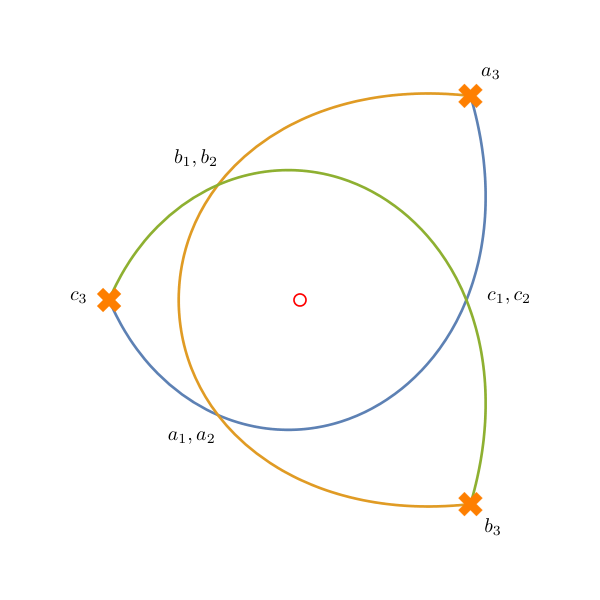
The fractional branes near the orbifold point are represented by the orange, green and blue finite webs respectively in Figure 29. The fractional branes and correspond to the simple representation with dimension vectors , and The central charges of the basic fractional branes are shown in Figure 29. For clarity, we have chosen a point in the complex structure moduli space where the central charges of the two fractional branes nearly align. This ensures that the resolutions of Lagrangian intersections will be localized close to the original intersection point. The central charges of these branes as a function of the complex structure modulus is relegated to Appendix B. Each pair of fractional branes intersect in three points. For each pair, one intersection point is at a branch point and two intersection points on come from the two distinct lifts of an intersection point on The resulting quiver is shown in Figure 27.
Kronecker-3 Quiver
We first consider bound states of two of the two fractional branes and . The quiver quantum mechanics reduces to the Kronecker-3 subquiver consisting of three arrows between the nodes and We label the intersection at the bottom branch point by and label the two intersection points near the top center by ‘’ and ‘’. This is the same labelling scheme for the Kronecker-3 quiver used in Figure 10. As explained in section 2.3, resolving intersections corresponds to giving a VEV to the corresponding fields in the quiver quantum mechanics. The notation in the figures to come is explained in the next subsection.
We start by considering bound states corresponding to representations with dimension vector . The moduli space of representations is . This moduli space has three torus fixed points and accordingly the Euler characteristic is three. For each of the three torus fixed points there is a corresponding finite web. The finite webs are shown in figures 30(a) and 30(b). The finite web shown in Figure 30(a), resolves the intersection in the top center by either a or a strand. The two possible resolutions correspond to two distinct finite webs contributing two to the Euler characteristic. Depending on the choice of resolution a VEV is given to the ‘’- or ‘’-arrow in the Kronecker-3 quiver corresponding to the or strand. The second finite web, Figure 30(b), detaches a strand from the bottom intersection point, giving a VEV to the third B-arrow in the Kronecker quiver. Note that there is a continuous family of finite webs interpolating between the three distinguished members: it is possible to gradually shorten the link to zero size, simultaneously detaching the strands at the bottom branch point. The link can then be regrown with a strand. This does not quite match the moduli space, though it is reminiscent of its toric diagram.


The moduli space for the dimension vector is again . We again find three finite webs corresponding to the three torus fixed points. The first finite web shown in Figure 31(a) resolves the top intersection by a strand. The corresponding “abelianized” quiver representation is shown in Figure 33. The other two finite webs shown in Figure 31(b) resolve the top intersection point by a or strand. Note that of the two strands starting from the top left branch point in figure 31(b), only one of them goes around the loop, and collides with the one that didn’t get to make a strand offspring. The quiver representation corresponding to resolving by a strand is shown in Figure 33. Less obvious than in the previous case, there is also a family of finite webs interpolating the two pictures, obtained by resolving the 4-way junction in figure 31(b).
From tree modules to networks
We now explain how to obtain representations of the Kronecker-3 quiver from exponential networks. In section 3.3 we described a special family of quiver representations for dimension vector of the Kronecker-3 quiver in terms of tree modules, where is the -th Fibonacci number. We now wish to exhibit exponential networks corresponding to these representations.
To simplify the translation, and reduce the clutter, we will use an alternative notation that first appeared in Figure 7. In the new notation, there is one label for each copy of the original basic states that make up the bound state. Every label follows a strand that starts and ends where the corresponding basic state did, possibly traveling through resolutions and possibly ending detached from the branch point. Note that the number of labels on a strand is not necessarily equal to its multiplicity. Rather, it can be recovered from the conversions shown in Figures 34(a) and 34(b). We will from now on refer to strands born according to reactions 4.6 and 4.7 as and strands respectively. The conversion rules might be best illustrated on a sample network of sufficient complexity. To this end, we show the fully labelled representation of the Kronecker-3 quiver realized on local , in the “old” -notation in Fig. 40, and in the new notation in Fig. 41.


Tree modules can be described in terms of a covering quiver of the original quiver representation. They bear a striking resemblance to quantum Hall halos [54]. In the covering quiver of the Kronecker-3 quiver we will always orient the arrows such that is in the vertical direction and ‘’/‘’ are at 120 degrees to B. These conventions are easily illustrated in Figure 35. Giving a covering quiver representation, we slice it horizontally into string modules by forgetting the vertical ‘B’ arrows. The resulting collection of quivers will correspond to representations of the Kronecker-2 quiver with the two arrows corresponding to ‘’ and ‘’. Each time there is a representation of the Kronecker-2 quiver with copies of meeting copies of we will associate a strand to the resolution of the corresponding intersection. This translation agrees with the representation that we gave in Figure 33 for the finite web shown in Figure 31(a). In the odd Fibonacci case the covering quiver has a left-right asymmetry and there will be additional or strands to resolve the ambiguities.

The representation for dimension vector has as its moduli space. Therefore there is a single torus fixed point which is represented by a single finite web shown in Figure 36. There is a single 2:1 strand resolving the top intersection point and one of the strands detaches from the bottom branch point. The corresponding quiver representation appears in equation (3.14) and Figure 35 illustrates the rules for converting between a finite web and its associated tree module.
More exotic Fibonacci representations
We now turn to the and Fibonacci representations. There are three families of tree modules corresponding to the three torus fixed points for the representation vector . The representation shown in Figure 39 corresponds to a finite web with a resolution by a 3:2 strand and two strands detaching from the bottom branch point. There indeed is such a finite web and it is shown in Figure 39.
There is a second type of representation shown in Figure 39. The corresponding finite web is show in Figure 41 (as well as in Fig. 40 in the “old” notation). An interesting feature is the or strand that determines if the arrow between the nodes ‘e’ and ‘g’ is a ’+’ or a ’-’.

Finally we consider the representation shown in Figure 42. The moduli space is again a single point and there is one finite web. The network is shown in Figure 43.

6.2 Large volume
At large volume the brane charges are linear combinations of the D0, D2 and D4 brane charges. The branes with compact support can be mathematically described as sheaves on . The compact part of the moduli space of the D0 brane is . There are three finite webs corresponding to the fixed points. They appear in Figure 44; one is attached to the leftmost branch point, while the other two arise from the piece of network with a or strand.
The webs corresponding to the D0- and D4- branes are shown in Figure 44. The figure is drawn at a point in moduli space where the central charges of the D0- and D4-branes align. The D4-brane corresponds to the network consisting of a single strand connecting two branch points. The D4-brane becomes massless at the conifold point, and grows to infinite size towards large volume.

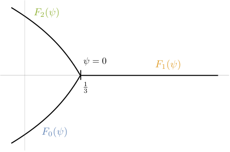
Finally we consider a D2-brane brane near the large volume point. In the orbifold basis it has charge . From Figure 45(a), we see that it becomes massless at the orbifold point. However the CFT is non-singular there so we expect that the D2-brane decays somewhere on the way from large volume. Figure 45 also provides a natural suggestion for the location and mechanism of the decay, namely that the D2-brane decays to objects with charges and on the locus where the periods and anti-align [12]. We get a very nice visual corroboration of this fact by plotting the networks, as shown in Figure 46.

A natural avenue for further study is transporting the Fibonacci representations from near the orbifold point to the large volume point. These should correspond to the mirrors of Fibonacci bundles [64] on the mirror of local
7 Flat Space
7.1 Quiver

The compact spectrum of consists only of the D0-brane. The network is shown in Figure 47, more fully decorated in Figure 48, 55 5 In this section we plot in a variable such that the puncture at lies at finite distance. As a visual benefit Figure 47 is easily recognized as a subset of Figure 44. and rendered on in Figure 49. There are three self-intersection points in the network. One intersection is at the branch point. The intersection point at the left in Figure 47 lifts to two intersection points on These three intersection points have the same orientation and are the matter fields in the quiver with a single vertex and three loops shown in Figure 50. The superpotential arises from the two holomorphic disks with opposite orientation shown in Figure 49.

Higher framing
As a brief consistency check we verify that the D0 brane exists at higher framing and that its mass is independent of the framing. Figure 51 shows the D0 brane at a framing such that the mirror curve is cubic in . The additional self-intersection points on are absent on because the strands lift to different sheets.
Moduli of the D0-brane

The finite web corresponding to the fixed point D0 brane has the following moduli available for deformation. The first modulus is detaching the finite web from its branch point anchor, i.e. moving it towards the waist in the pair of pants shown in Figure 49. The second modulus is to resolve the left intersection point by opening a strand according to the junction rule. The resulting moduli space is drawn in Figure 52. A generic web with both moduli turned on is shown as a member of the fat strip in Figure 52. The size of that strand is arbitrary and can be grown until it eats up the entire finite web. If the finite web is attached to the branch point, the bubble can detach on the other side as shown along both edges in Figure 52, which corresponds to moving towards on one of the legs. Note that the vertical reflection symmetry implements the interchange of and in both figures.
Alice: How long is forever?
White Rabbit: Sometimes, just one second.
7.2 Mirror ADHM moduli spaces
Non-compact branes
In this section, we describe non-compact D2- and D4-branes. The D4-brane is represented by the strand starting from the branch point running into the puncture at . We regularize its central charge by cutting the strand at some large finite mass. Non-compact D4-branes can be used to geometrically engineer framed BPS states [65].
Evidence for this identification includes the divergence of the central charge as (see (4.5)), two oppositely oriented intersections with the D0-brane giving rise to the ADHM quiver in Figure 9 66 6 The two extra intersections give rise to the fields and in the ADHM quiver. The extra holomorphic disk modifies the potential to The F-term relations for the field reduce to the ADHM relations after replacing and by and ., and a compact model in the large volume region of local , see Figure 44. In a similar way, we identify the strand starting at the branch point and going into the puncture as a non-compact D2-brane: the central charge diverges as and we can also recognize it as a decompactified limit of the D2 brane on the resolved conifold (see also (4.3)).
In addition to complexified Kähler moduli, on local Calabi-Yau one should also keep track of the B-field in non-compact directions. If B-fields are turned on in the directions parallel to the D4 brane, then to leading order in the B-field the phase its central charge will be given by . We use this to identify the B-field with the phase at which the D4 brane exists, see Figure 53.
D0-D4 bound states
Now we consider bound states of the non-compact D4-brane with D0-branes. The central charge of the D0 brane is independent of the B-field, so at nonzero B-field the bound states of the D0 and the D4 have distinct phases and are nicely separated. The bound state of the D4 brane with a D0 brane is shown in Figure 54. The regularization is enforced by imposing that the diverging strand ends at precisely the same point as the pure D4 (in practice, we simply ‘‘shoot’’ backwards from that point). The regularized central charge obeys the usual additivity77 7 This additivity of the central charge holds for open segments in general, whether they are near or not. In general an open segment could be interpreted as an open brane or a “soliton” in the sense of [5], and can also form bound states with D0 branes. This is a natural avenue for future research..
The moduli space of D0-branes sitting inside coincident D4 branes is isomorphic to the moduli space of -instantons in Yang-Mills [66, 67]. However this holds at zero B-field, so the bound states all occur at the same phase hence are not readily studied. For there are no instantons in pure Yang-Mills, but as explained in [68] the inclusion of a B-field into the problem maps to a non-commutative deformation of the gauge theory, which does admit instantons precisely for . This problem is also related to the representations of the Nakajima quiver described in section 3.3, and we now make the connection with spectral networks.
According to Nakajima’s theorem, and following our identification of finite webs with toric fixed points in moduli space, we should be able to associate a finite web corresponding to a bound state of the D4 and D0 branes to each partition of . As a guiding principle in this quest we postulate the row-column duality on Young diagrams is implemented on finite webs by exchanging all and strands.
Figures 55 through 58 show finite webs corresponding to bound states of the D4 brane with a small number of D0 branes. The connection to covering quivers appears to work in a similar way as for the Kronecker-3 quiver described earlier. Nonzero entries of the and matrices correspond to a connection between basic constituents of the bound state (here, the D4 brane and each separate D0 brane). We identify a left-right symmetry breaking arrow in the covering quiver with a connection through a or strand. The labels in the diagrams indicate the connection structure. In this section instead of colors we use the label for a strand born of strands with labels and .
“and what is the use of a book,” thought Alice,
“without pictures or conversations?”


The bound state of the D4 with two D0’s is shown in Figure 55. There is a single or strand that resolves the intersection corresponding to or The choice determines whether the corresponding partition is (2) and (1,1) which are transposes of each other.
| (7.1) |
The finite web for the (2,1) partition of 3 is shown in Figure 56. The covering quiver is left-right symmetric and accordingly there is no or strand, only a strand.
| (7.2) |
The finite webs for partitions (3) and (1,1,1) of are shown in Figure 57, where the resolutions are either both or .
| (7.3) |
Recall that the and matrices obtained from the covering quiver satisfy the -term relation by construction. Mnemonically the -term relation is equivalent to stability of the covering quiver if it is lying on a wedge and gravity points down the page. We use this condition to eliminate many finite webs, including the one in Figure 57 with a mixed labeling of and .
The partitions of of type row or column generalize easily to a family of finite webs with strands of type or . The finite web for those partition of is shown in Figure 58.
| (7.4) |
The finite web for the square partition, (2,2), of 4 is shown in Figure 59. There is a strand corresponding to followed by a strand , consistent with the decomposition of the covering quiver. There are no or strands since the (2,2) partition is its own transpose.
| (7.5) |
Why, sometimes I’ve believed as many as six impossible things before breakfast. (The Queen of Hearts)

The partition (3,1) of 4 is the first one to which we do not know how to associate a finite web. There is a reasonable looking candidate shown in Figure 60, but the associated covering quiver does not satisfy the -term relation.

Imagination is the only weapon in the
war against reality. (The Cheshire Cat)
8 Conclusions
In this paper, we have studied the geometric B-model description of BPS states in theories admitting a spectral curve parametrization. One of our main results is a direct and systematic relationship between geodesic networks and quiver representations arising from tachyon condensation. Although our main focus has been on “exponential networks” capturing BPS spectra of local Calabi-Yau manifolds, our method also produces new results for the ordinary spectral networks of Gaiotto-Moore-Neitzke. (A related way of associating representations to homotopy classes of WKB geodesics in triangulated surfaces appears in [43, 69, 42].) We hope that a complete understanding of the translation between quiver representations and WKB geodesics will eventually resolve the matching between partitions and networks in Section 7.2.
Although we have seen that many of the constructions from [3, 5] can be extended to the mirrors of local Calabi-Yau manifolds, there are many other aspects of spectral networks that should have interesting generalizations to exponential networks. In Section 7.2, we have identified the mirror of non-compact D2- and D4-branes with non-compact cycles on the Riemann surface. These branes can be used to study coupled 3d-5d wall-crossing in a way similar to [70]. Another generalization is to extract spin content from an exponential network, revealing information about the Hodge polynomial of the moduli space of the corresponding quiver quantum mechanics [71]. Finally, exponential networks can be used to lift 4d gauge theory BPS state counting problems to 5d gauge theory BPS state counting problems. An example of this type of lift is the generalization from non-relativistic integrable systems to relativistic integrable systems. Spectral networks corresponding to the periodic nonrelativistic Toda system were used to compute traces of holonomies on the associated cluster variety [72]. Applying the construction of [73] to the local Calabi-Yau manifolds results in a family of generalized periodic relativistic Toda systems [74]. It would be interesting to give a string-theoretic derivation of the Goncharov-Kenyon integrable systems [73] using exponential networks.
One of the most promising avenues is giving concrete B-model descriptions of phenomena mirror to well-known A-model constructions. For instance, it should be possible to give a mirror description of the Betti numbers of the moduli space of sheaves on [75, 76] using exponential networks. A more intriguing challenge is to see if there is a B-model explanation for the appearance of mock-modularity in these moduli problems. Perhaps the most pressing challenge is to find a description of the D6-brane on the spectral curve side and its effect on the stability of exponential networks. One of the characteristic properties of the D6-brane is that it does not arise as the boundary of any A-brane. Therefore, it seems unlikely that the mirror of a D6-brane would be a one-dimensional submanifold of the spectral curve since any such trajectory could always be terminated at a point on the curve and therefore would in fact bound a B-brane. We suspect that for a concrete mirror version of Donaldson-Thomas theory in the local case, one will have to reckon with a description of the framing that is non-geometric on the spectral curve.
Finally, there should be a direct proof of the Kontsevich-Soibelman wall-crossing formula [2] for the mirrors of local Calabi-Yau manifolds directly in terms of exponential networks similar to the one in [5].
Acknowledgments We thank Murad Alim for extensive discussions on the material in section 7 and for collaboration on a related project. We also thank Heeyeon Kim, Wolfgang Lerche, Andy Neitzke, and Nick Warner for valuable discussions. The work of S.S. was supported in part by a Grant from the FQRNT (Fonds Québécois de Recherche - Nature et Technologies).
Appendix A Coding Advice for Exponential Networks
Recall from equation 4.1 the differential
| (A.1) |
where the is the -th local solution of . We now explain some details of solving for the integral geodesics of equation (4.2)
| (A.2) |
numerically. Let and absorb the into the choices of branch cuts. Then in these variables, equation (A.2) becomes
| (A.3) |
Locally, away from a branch point, the system of equations
| (A.4) |
determine the local evolution of the network. However, at a branch point, the lifts coincide, and Therefore a more careful analysis is necessary. Consider the covering of by around a branch point of order
| (A.5) |
We rearrange the equation as
| (A.6) |
where
| (A.7) |
For simplicity, we now restrict our attention to when . Solving for ,
| (A.8) |
where . We then have the approximation
| (A.9) |
Substituting into equation (A.3), we have
| (A.10) |
Integrating from to , we have
| (A.11) |
Solving for
| (A.12) |
To solve for with a consistent choice of branches, we use the following trick:
| (A.13) |
We substitute this into
| (A.14) |
The analysis for coverings of higher degree is similar.
Appendix B Central Charges of Local Calabi-Yau Manifolds
B.1 Orbifold point
Near the orbifold point, we switch to the coordinate where Then a basis of solutions to the Picard-Fuchs equation is
| (B.2) |
where The central charges of the fractional branes near the orbifold point are given by
| (B.3) |
and are plotted in Figure 45(a).
B.2 Large volume solutions
Appendix C Representations of Quivers with Superpotential
In section 5 we used the folklore result that the representation theory of the conifold quiver effectively reduces to the representation theory of the Kronecker-2 quiver. This means that either only the “A” or only the “B” arrows can be non-zero in an indecomposable representation of the conifold quiver, except for when the dimension vector is a multiple of . We justify this statement in the simple case of dimension vector . For other representations, the analysis is similar but more involved. For local a similar analysis was performed in [12]. In general, it is natural to conjecture that only the representations corresponding to the D0-brane involve all of the fields in the quiver. For local Calabi-Yau manifolds that arise as cones over surfaces, the representations are expected to restrict to representations of an acyclic quiver corresponding to the surface. In the example of local either the or fields will be zero in a representation not corresponding to the D0-brane, reducing the representation theory to that of the Beilinson quiver for .
Recall that the conifold quiver has superpotential and F-term (Jacobian) equations
| (C.1) |
We consider a representation with dimension vector . Then a representation will take the form
| (C.2) |
When expanded out in components, the first two F-term relations yield
| (C.3) |
where . Thus either or If , then using the remaining two F-term equations, we find or So either or or . In the first case, we are in the situation we wished to show, that either the or fields are zero. The other case where corresponds to a bound state of a and representation. This follows from the fact that implies that the common image of the maps from to is only one dimensional.
References
- [1] F. Denef and G. W. Moore, “Split states, entropy enigmas, holes and halos,” JHEP 1111, 129 (2011) [arXiv:hep-th/0702146].
- [2] M. Kontsevich and Y. Soibelman, “Stability structures, motivic Donaldson-Thomas invariants, and cluster transformations” (2008) arXiv:0811.2435 [math.AG]
- [3] D. Gaiotto, G. W. Moore and A. Neitzke, “Four-dimensional wall-crossing via three-dimensional field theory,” Commun. Math. Phys. 299, 163 (2010) arXiv:0807.4723 [hep-th].
- [4] D. Gaiotto, G. W. Moore and A. Neitzke, “Wall-crossing, Hitchin Systems, and the WKB Approximation,” arXiv:0907.3987 [hep-th].
- [5] D. Gaiotto, G. W. Moore and A. Neitzke, “Spectral networks,” Annales Henri Poincare 14, 1643 (2013) [arXiv:1204.4824 [hep-th]].
- [6] H. Ooguri, A. Strominger and C. Vafa, “Black hole attractors and the topological string,” Phys. Rev. D 70, 106007 (2004) [arXiv:hep-th/0405146].
- [7] A. Klemm, W. Lerche, P. Mayr, C. Vafa and N. P. Warner, “Selfdual strings and N=2 supersymmetric field theory,” Nucl. Phys. B 477, 746 (1996) [arXiv:hep-th/9604034].
- [8] V. Batyrev and L.A. Borisov, “Dual cones and mirror symmetry for generalized Calabi-Yau manifolds,” (1994) arXiv:alg-geom/9402002
- [9] K. Hori and C. Vafa, “Mirror symmetry,” arXiv:hep-th/0002222.
- [10] M. Aganagic and C. Vafa, “Mirror symmetry, D-branes and counting holomorphic discs,” arXiv:hep-th/0012041.
- [11] V. Bouchard, A. Klemm, M. Marino and S. Pasquetti, “Remodeling the B-model,” Commun. Math. Phys. 287, 117 (2009) [arXiv:0709.1453 [hep-th]].
- [12] M. R. Douglas, B. Fiol and C. Romelsberger, “The Spectrum of BPS branes on a noncompact Calabi-Yau,” JHEP 0509, 057 (2005) [arXiv:hep-th/0003263].
- [13] S. Cecotti and C. Vafa, “Classification of complete N=2 supersymmetric theories in 4 dimensions,” Surveys in differential geometry 18 (2013) , arXiv:1103.5832 [hep-th].
- [14] M. Alim, S. Cecotti, C. Cordova, S. Espahbodi, A. Rastogi and C. Vafa, “BPS Quivers and Spectra of Complete N=2 Quantum Field Theories,” Commun. Math. Phys. 323, 1185 (2013) [arXiv:1109.4941 [hep-th]].
- [15] P. Seidel, “Homological mirror symmetry for the genus two curve,” J. Algebraic Geom. 20, 727–769 (2011)
- [16] D. Auroux, L. Katzarkov and D. Orlov, “Mirror symmetry for del Pezzo surfaces: Vanishing cycles and coheren sheaves,” Invent. Math. 166, 537–582 (2006)
- [17] W. Lerche, “Introduction to Seiberg-Witten theory and its stringy origin,” Nucl. Phys. Proc. Suppl. 55B, 83 (1997) [Fortsch. Phys. 45, 293 (1997)] [arXiv:hep-th/9611190].
- [18] K. Dasgupta and S. Mukhi, “BPS nature of three string junctions,” Phys. Lett. B 423, 261 (1998) [arXiv:hep-th/9711094].
- [19] S. Selmani, work in progress.
- [20] N. Seiberg and E. Witten, “Electric - magnetic duality, monopole condensation, and confinement in N=2 supersymmetric Yang-Mills theory,” Nucl. Phys. B 426, 19 (1994) Erratum: [Nucl. Phys. B 430, 485 (1994)] [arXiv:hep-th/9407087].
- [21] J. Walcher, “Stability of Landau-Ginzburg branes,” J. Math. Phys. 46, 082305 (2005) [arXiv:hep-th/0412274].
- [22] W. Lerche, P. Mayr and N. P. Warner, “Noncritical strings, Del Pezzo singularities and Seiberg-Witten curves,” Nucl. Phys. B 499, 125 (1997) [arXiv:hep-th/9612085].
- [23] V. Bouchard, A. Klemm, M. Marino and S. Pasquetti, “Remodeling the B-model,” Commun. Math. Phys. 287 (2009) 117 [arXiv:0709.1453 [hep-th]].
- [24] B. Eynard and N. Orantin, “Invariants of algebraic curves and topological expansion,” Commun. Num. Theor. Phys. 1, 347 (2007) [arXiv:math-ph/0702045].
- [25] M. Aganagic, A. Klemm and C. Vafa, “Disk instantons, mirror symmetry and the duality web,” Z. Naturforsch. A 57, 1 (2002) [arXiv:hep-th/0105045].
- [26] M. R. Douglas and G. W. Moore, “D-branes, quivers, and ALE instantons,” arXiv:hep-th/9603167.
- [27] H. Nakajima, “Instantons on ALE spaces, quiver varieties, and Kac-Moody algebras,” Duke Math. J. 76 (1994), no. 2, 365–416.
- [28] P. B. Kronheimer and H. Nakajima, “Yang-Mills instantons on ALE gravitational instantons,” Math. Ann. 288 (1990) 263.
- [29] V. Kac, “Infinite root systems, representations of graphs and invariant theory,” Invent. Math., 56 (1980), pp. 57-92
- [30] P. Gabriel, “Unzerlegbare Darstellungen. I.”, Manuscripta Math. 6, 71-103 (1972).
- [31] M. R. Douglas, B. Fiol and C. Romelsberger, “Stability and BPS Branes,” JHEP 0509 (2005) 006 [arXiv:hep-th/0002037].
- [32] I. Assem, D. Simson, A. Skowroński, “Elements of the representation theory of associative algebras, Vol. 1” London Mathematical Society Student Texts 65, CUP (2006)
- [33] R. Schiffler, “Quiver representations,” CMS Books in Mathematics/Ouvrages de Mathématiques de la SMC, Springer (2014)
- [34] A.D. King, “Moduli of representations of finite-dimensional algebras,” Quart. J. Math. Oxford Ser. (2) 45, 515–530 (1994)
- [35] S. Kachru and J. McGreevy, “Supersymmetric Three Cycles and Supersymmetry Breaking,” Phys. Rev. D 61 (2000) 026001 [arXiv:hep-th/9908135].
- [36] B. Fiol and M. Mariño, “BPS States and Algebras from Quivers,” JHEP 0007 (2000) 031 [arXiv:hep-th/0006189].
- [37] K. Hori, A. Iqbal and C. Vafa, “D-branes and mirror symmetry,” arXiv:hep-th/0005247.
- [38] M. C. R. Butler and C. M. Ringel, “Auslander-Reiten sequences with few middle terms and applications to string algebras,” Comm. Algebra 15 no. 1-2, (1987) 145–179.
- [39] K. Becker, M. Becker and A. Strominger, “Five-Branes, Membranes and Nonperturbative String Theory,” Nucl. Phys. B 456 (1995) 130 [arXiv:hep-th/9507158].
- [40] H. Ooguri, Y. Oz and Z. Yin, “D-Branes on Calabi-Yau Spaces and Their Mirrors,” Nucl. Phys. B 477 (1996) 407 [arXiv:hep-th/9606112].
- [41] K. Fukaya, Y.-G. Oh, H. Ohta, and K. Ono, Lagrangian intersection Floer theory: anomaly and obstruction. Part I, vol. 46 of AMS/IP Studies in Advanced Mathematics. American Mathematical Society, Providence, RI; International Press, Somerville, MA, 2009.
- [42] S. Cecotti, “Categorical Tinkertoys for Gauge Theories,” Int. J. Mod. Phys. A 28 (2013) 1330006 [arXiv:1203.6734 [hep-th]].
- [43] I. Assem, T. Brüstle, G. Charbonneau-Jodoin, and P.-G. Plamondon, “Gentle algebras arising from surface triangulations,” Algebra Number Theory 4 no. 2, (2010) 201–229.
- [44] S. Fomin, M. Shapiro, and D. Thurston, “Cluster algebras and triangulated surfaces. I. Cluster complexes,” Acta Math. 201 no. 1, (2008) 83–146.
- [45] C. M. Ringel, “Exceptional modules are tree modules,” in Proceedings of the Sixth Conference of the International Linear Algebra Society (Chemnitz, 1996), vol. 275/276, pp. 471–493. 1998. http://dx.doi.org/10.1016/S0024-3795(97)10046-5.
- [46] T. Weist, “Tree modules of the generalised Kronecker quiver,” J. Algebra 323 no. 4, (2010) 1107–1138.
- [47] T. Weist, “Localization in quiver moduli spaces,” Represent. Theory 17 (2013) 382–425.
- [48] T. Weist, “On the Euler characteristic of Kronecker moduli spaces,” J. Algebraic Combin. 38 no. 3, (2013) 567–583.
- [49] H. Nakajima, Lectures on Hilbert schemes of points on surfaces, vol. 18 of University Lecture Series. American Mathematical Society, Providence, RI, 1999. http://dx.doi.org/10.1090/ulect/018.
- [50] P. Fahr and C. M. Ringel, “A partition formula for Fibonacci numbers,” J. Integer Seq. 11 no. 1, (2008) Article 08.1.4, 9.
- [51] P. Fahr and C. M. Ringel, “Categorification of the Fibonacci numbers using representations of quivers,” J. Integer Seq. 15 no. 2, (2012) Article 12.2.1, 12.
- [52] Leonardo of Pisa, “Liber Abaci,” (1202).
- [53] J. A. Harvey and G. W. Moore, “On the Algebras of BPS States,” Commun. Math. Phys. 197 (1998) 489 [arXiv:hep-th/9609017].
- [54] F. Denef, “Quantum Quivers and Hall / Hole Halos,” JHEP 0210 (2002) 023 [hep-th/0206072].
- [55] M. Reineke, “The Harder-Narasimhan system in quantum groups and cohomology of quiver moduli,” Invent. Math. 152 no. 2, (2003) 349–368.
- [56] F. Benini, R. Eager, K. Hori and Y. Tachikawa, “Elliptic Genera of Two-Dimensional Gauge Theories with Rank-One Gauge Groups,” Lett. Math. Phys. 104 (2014) 465 doi:10.1007/s11005-013-0673-y [arXiv:1305.0533 [hep-th]].
- [57] F. Benini, R. Eager, K. Hori and Y. Tachikawa, “Elliptic Genera of 2D = 2 Gauge Theories,” Commun. Math. Phys. 333 (2015) no.3, 1241 doi:10.1007/s00220-014-2210-y [arXiv:1308.4896 [hep-th]].
- [58] K. Hori, H. Kim and P. Yi, “Witten Index and Wall Crossing,” JHEP 1501 (2015) 124 doi:10.1007/JHEP01(2015)124 [arXiv:1407.2567 [hep-th]].
- [59] S. J. Lee and P. Yi, “Witten Index for Noncompact Dynamics,” JHEP 1606 (2016) 089 doi:10.1007/JHEP06(2016)089 [arXiv:1602.03530 [hep-th]].
- [60] H. Kim, “Scaling Behaviour of Quiver Quantum Mechanics,” JHEP 1507 (2015) 079 doi:10.1007/JHEP07(2015)079 [arXiv:1503.02623 [hep-th]].
- [61] C. Cordova and S. H. Shao, “Counting Trees in Supersymmetric Quantum Mechanics,” arXiv:1502.08050 [hep-th].
- [62] P. S. Aspinwall, B. R. Greene and D. R. Morrison, “Measuring Small Distances in Sigma Models,” Nucl. Phys. B 420 (1994) 184 [hep-th/9311042].
- [63] P. S. Aspinwall, “D-Branes, Pi-Stability and Theta-Stability,” hep-th/0407123.
- [64] M. C. Brambilla, “Cokernel bundles and Fibonacci bundles,” Math. Nachr. 281 no. 4, (2008) 499–516.
- [65] W. y. Chuang, D. E. Diaconescu, J. Manschot, G. W. Moore and Y. Soibelman, “Geometric Engineering of (Framed) BPS States,” Adv. Theor. Math. Phys. 18 (2014) no.5, 1063 [arXiv:1301.3065 [hep-th]].
- [66] E. Witten, “Sigma Models and the ADHM Construction of Instantons,” J. Geom. Phys. 15 (1995) 215 [hep-th/9410052].
- [67] M. R. Douglas, “Branes Within Branes,” In *Cargese 1997, Strings, branes and dualities* 267-275 [hep-th/9512077].
- [68] N. Seiberg and E. Witten, “String Theory and Noncommutative Geometry,” JHEP 9909 (1999) 032 [hep-th/9908142].
- [69] D. Labardini-Fragoso, “Quivers with potentials associated to triangulated surfaces, Part II: Arc representations,” ArXiv e-prints (Sept., 2009) , arXiv:0909.4100 [math.RT].
- [70] D. Gaiotto, G. W. Moore and A. Neitzke, “Wall-Crossing in Coupled 2D-4D Systems,” JHEP 1212 (2012) 082 doi:10.1007/JHEP12(2012)082 [arXiv:1103.2598 [hep-th]].
- [71] D. Galakhov, P. Longhi and G. W. Moore, “Spectral Networks with Spin,” Commun. Math. Phys. 340 (2015) no.1, 171 doi:10.1007/s00220-015-2455-0 [arXiv:1408.0207 [hep-th]].
- [72] H. Williams, “Toda Systems, Cluster Characters, and Spectral Networks,” Commun. Math. Phys. 348 (2016) no.1, 145 doi:10.1007/s00220-016-2692-x [arXiv:1411.3692 [math.RT]].
- [73] A. B. Goncharov and R. Kenyon, “Dimers and cluster integrable systems,” Ann. Sci. Éc. Norm. Supér. (4) 46 no. 5, (2013) 747–813.
- [74] R. Eager, S. Franco and K. Schaeffer, “Dimer Models and Integrable Systems,” JHEP 1206 (2012) 106 doi:10.1007/JHEP06(2012)106 [arXiv:1107.1244 [hep-th]].
- [75] K. Yoshioka, “The Betti numbers of the moduli space of stable sheaves of rank on a ruled surface,” Math. Ann. 302 no. 3, (1995) 519–540.
- [76] K. Yoshioka, “The Betti numbers of the moduli space of stable sheaves of rank on ,” J. Reine Angew. Math. 453 (1994) 193–220.
- [77] P. S. Aspinwall, “D-Branes on Calabi-Yau Manifolds,” arXiv:hep-th/0403166.
- [78] K. Hori and M. Romo, “Exact Results in Two-Dimensional (2,2) Supersymmetric Gauge Theories with Boundary,” arXiv:1308.2438 [hep-th].
- [79] D. Honda and T. Okuda, “Exact Results for Boundaries and Domain Walls in 2D Supersymmetric Theories,” JHEP 1509 (2015) 140 doi:10.1007/JHEP09(2015)140 [arXiv:1308.2217 [hep-th]].
- [80] S. Sugishita and S. Terashima, “Exact Results in Supersymmetric Field Theories on Manifolds with Boundaries,” JHEP 1311 (2013) 021 doi:10.1007/JHEP11(2013)021 [arXiv:1308.1973 [hep-th]].