Multi-User Millimeter Wave MIMO with Full-Dimensional Lens Antenna ArrayThanks: The authors are with the Department of Electrical and Computer Engineering, National University of Singapore (e-mail: {elezeng, eleylu, elezhang}@nus.edu.sg).Thanks: Part of this paper has been submitted to the IEEE International Conference on Communications (ICC), May 21-25, 2017, Paris, France.
Abstract
Millimeter wave (mmWave) communication by utilizing lens antenna arrays is a promising technique for realizing cost-effective 5G wireless systems with large MIMO (multiple-input multiple-output) but only limited radio frequency (RF) chains. This paper studies an uplink multi-user mmWave single-sided lens MIMO system, where only the base station (BS) is equipped with a full-dimensional (FD) lens antenna array with both elevation and azimuth angle resolution capabilities, and each mobile station (MS) employs the conventional uniform planar array (UPA) without the lens. By exploiting the angle-dependent energy focusing property of the lens antenna array at the BS as well as the multi-path sparsity of mmWave channels, we propose a low-complexity path division multiple access (PDMA) scheme, which enables virtually interference-free multi-user communications when the angle of arrivals (AoAs) of all MS multi-path signals are sufficiently separable at the BS. To this end, a new technique called path delay compensation is proposed at the BS to effectively transform the multi-user frequency-selective MIMO channels to parallel frequency-flat small-size MIMO channels for different MSs, for each of which the low-complexity single-carrier (SC) transmission is applied. For general scenarios with insufficient AoA separations, analog beamforming at the MSs and digital combining at the BS are jointly designed to maximize the achievable sum-rate of the MSs based on their effective MIMO channels resulting from path delay compensation. In addition, we propose a new and efficient channel estimation scheme tailored for PDMA, which requires negligible training overhead in practical mmWave systems and yet leads to comparable performance as that based on perfect channel state information (CSI). Numerical results show that the proposed design significantly outperforms state-of-the-art benchmark systems in terms of sum-rate, but with significantly reduced hardware cost and signal processing complexity.
Index Terms:
Millimeter wave communication, MIMO, lens antenna array, path division multiple access (PDMA), analog beamforming, channel estimation.I Introduction
Due to the large bandwidth available, millimeter wave (mmWave) communication over the spectrum above 28GHz has emerged as a key enabling technology for the fifth-generation (5G) wireless systems [1, 2, 3, 4, 5]. In fact, mmWave systems at the unlicensed 60GHz have already been standardized for short-range applications, such as wireless personal area networks (WPAN) [6] and wireless local area networks (WLAN) [7]. In July 2016, the FCC (Federal Communications Commission) of the United States has released 3.85GHz of licensed and 7GHz of unlicensed mmWave frequency spectrum for future broadband communications [8], which made an important step forward for mmWave technology to be practically employed for mobile access in 5G.
Compared to the conventional sub-6GHz wireless systems, mmWave communications are faced with many new design challenges [9]. In particular, to maintain a sufficient link margin for signal coverage at a reasonable range, mmWave systems typically require large antenna arrays (in terms of the number of array elements) to be equipped at the base station (BS), and also possibly at each mobile station (MS), to achieve highly directional communications. While packing more antennas compactly with small form factors is becoming more feasible at mmWave frequencies, thanks to the significantly reduced wavelength, the associated signal processing complexity and radio frequency (RF) chain cost in terms of hardware and power consumption increase dramatically, if the conventional multiple-input multiple-output (MIMO) communication techniques are used. Furthermore, due to the large signal bandwidth, mmWave systems are most likely to operate over frequency-selective channels, for which the detrimental inter-symbol interference (ISI) needs to be effectively mitigated. However, ISI mitigation is a non-trivial task for wide-band mmWave large MIMO systems, especially for practical designs that need to operate with low signal processing complexity and RF chain costs, due to which the traditional ISI mitigation techniques such as MIMO-OFDM (orthogonal frequency division multiplexing) and sophisticated time/frequency-domain equalizations become less effective.
Extensive research efforts have been devoted to developing various cost-aware mmWave communication techniques, such as analog beamforming [10, 11, 12], hybrid analog/digital processing [13, 14, 15, 16, 17, 18, 19, 20], and low-resolution ADCs (analog to digital converters) for signal reception [21]. In particular, hybrid analog/digital processing is regarded as an effective technique to offer flexible trade-offs between performance and cost by varying the number of RF chains at the transmitter/receiver. With this technique, the signal processing is implemented via two stages: a low-dimensional baseband digital processing using limited number of RF chains concatenated with an RF-band analog processing through a network of phase shifters. In [15], the hybrid precoding and combining matrices are optimized for single-user narrow-band mmWave systems based on the concept of orthogonal matching pursuit, and its extensions to codebook-based multi-user frequency-flat and single-user frequency-selective MIMO-OFDM systems are studied in [16] and [17], respectively. In [18], it has been shown that for narrow-band systems, hybrid processing is able to achieve the same performance as the fully digital processing scheme, provided that the number of RF chains is at least twice of the number of data streams. Channel estimation for mmWave hybrid systems has also been investigated in [19] and [20]. However, one major drawback of the hybrid analog/digital architecture is the general requirement of an extremely large number of phase shifters, which consume extra power that may even outweigh the power saving due to the use of fewer RF chains. Besides, due to the additional constant-amplitude constraints on the analog beamformers as well as the limited RF chains available, the precoding/combining design as well as channel estimation for hybrid processing is more complicated than the conventional fully digital design, especially for wide-band systems with frequency-selective channels [17], [20].
Another line of researches has focused on achieving cost-effective mmWave communications by utilizing the advanced lens antenna arrays [22, 23, 24, 25, 26, 27, 28, 29]. A lens antenna array is in general composed of an electromagnetic (EM) lens with energy focusing capability, and a matching antenna array with elements located in the focal region of the lens. In [25], it is derived that the array response of a lens antenna array can be expressed as a “sinc”-type function in terms of the angle of arrival/departure (AoA/AoD) and the antenna locations, which theoretically confirms the angle-dependent energy focusing property of lens antenna arrays, i.e., for each uniform plane wave of a given AoA/AoD, only those antennas located in the close vicinity of the energy focusing point receives/steers significant power. By exploiting this unique array response, together with the multi-path sparsity of mmWave channels [3], a new spatial multiplexing technique, termed path division multiplexing (PDM), is proposed in [25] for the point-to-point mmWave MIMO channel, which is capacity-achieving using the simple single-carrier (SC) transmission with low RF chain cost and signal processing complexity, even for wide-band frequency-selective mmWave communications. MmWave lens MIMO systems have also been shown be able to effectively reduce the channel estimation overhead as compared to hybrid processing systems subject to limited number of RF chains [27].
However, most existing works on mmWave lens MIMO consider only the single-user systems with double-sided lenses, i.e., by assuming lens antenna arrays at both the BS and MS. Due to the additional gap required between the EM lens and antenna elements, lens antenna array is expected to be more suitable to be employed at the BS than at the MS, which has more stringent size limitations in practice. Besides, existing lens array designs mostly ignore the signal’s elevation angles, and thus consider only the two-dimensional (2D) array with antenna elements located in the focal arc only. In this paper, we consider a more general setup of multi-user mmWave lens MIMO system with single-sided full-dimensional (FD) lens antenna array, i.e., only the BS is equipped with an FD lens antenna array with both azimuth and elevation angle resolution capabilities, while each MS employs the conventional antenna array such as the uniform planar array (UPA) without the lens. Under such a new setup and with limited RF chains at the BS and one single RF chain at each MS, we propose a low-complexity transceiver design for general multi-user wide-band mmWave communications in frequency-selective channels, as well as an efficient channel estimation scheme with nearly negligible training overhead. The specific contributions of this paper are summarized as follows.
- •
First, we introduce the general architecture for FD lens antenna arrays. Different from the 2D lens array studied in our prior work [25], the array elements of FD lens array are located in the focal surface (instead of focal arc) of the lens and thus offer both elevation and azimuth angle resolution capabilities. We further derive the array response vector of the FD lens antenna array, which is shown to be given by the product of two “sinc” functions reflecting the elevation and azimuth angle resolutions, respectively.
- •
Next, we study the uplink multi-user mmWave single-sided FD lens MIMO system with limited RF chains at the BS and one single RF chain at each MS. By exploiting the unique array response of the FD lens array at the BS, together with the multi-path sparsity of mmWave channels, we propose a low-complexity path division multiple access (PDMA) scheme that is applicable for the general frequency-selective channels. With PDMA, the MSs essentially communicate with the BS via different channel paths without incurring any ISI or inter-user interference (IUI), as long as the AoAs of all MS multi-paths are sufficiently separable at the BS. To this end, a new technique called path delay compensation is proposed to effectively transform the multi-user frequency-selective MIMO channels to parallel frequency-flat small-size MIMO channels for different MSs, for each of which the low-complexity SC transmission can be applied. For general scenarios where the AoAs cannot be fully separated at the BS, analog beamforming at the MSs and digital combining at the BS are jointly designed to maximize the sum-rate of all MSs with the MRC (maximal ratio combining) and MMSE (minimum mean square error) based combining, respectively.
- •
Last, we propose a new and efficient channel estimation scheme tailored for PDMA, which consists of three phases, namely power-based antenna selection, path estimation and association, and reduced effective MIMO channel estimation. Thanks to the angle-dependent energy focusing of lens array at the BS and the low-complexity of PDMA, the proposed channel estimation scheme incurs very small training overhead in practical mmWave systems and leads to comparable performance as that based on perfect channel state information (CSI). Numerical results are provided to show the effectiveness of the proposed designs, and their sum-rate performance compared to state-of-the-art benchmark systems.
The rest of this paper is organized as follows. Section II introduces the general FD lens antenna arrays as well as the system model of multi-user single-sided lens MIMO. In Section III, we propose the PDMA scheme as well as the MRC- and MMSE-based beamforming designs. In Section IV, an efficient channel estimation scheme tailored for the proposed PDMA scheme is presented. Numerical results are given in Section V. Finally, we conclude the paper in Section VI.
Notations: In this paper, scalars are denoted by italic letters. Boldface lower- and upper-case letters denote vectors and matrices, respectively. denotes the space of complex-valued matrices, and represents an identity matrix. For an arbitrary-size matrix , its complex conjugate, transpose, and Hermitian transpose are denoted by , , and , respectively. For a vector , denotes its Euclidean norm. For a non-singular square matrix , its matrix inverse is denoted as . The symbol represents the imaginary unit of complex numbers, with . The notation denotes the linear convolution operation. denotes the Dirac delta function, and is the “sinc” function defined as . For a real number , and denote the floor and ceiling operations, respectively. Furthermore, denotes the circularly symmetric complex-valued Gaussian (CSCG) distributions with mean and covariance matrix . For a set , denotes its cardinality. Furthermore, , and denote the intersection, union, and complement of two sets and , respectively.
II System Model
II-A Full-Dimensional Lens Antenna Array
Fig. 1 gives a schematic illustration of a lens antenna array in three-dimensional (3D) coordinate system, which consists of a planar EM lens with negligible thickness in the y-z plane centered at the origin, together with the antenna elements located in the focal surface of the EM lens. Let and denote the electric dimensions of the lens (i.e., the physical dimensions normalized by signal wavelength) along the y- and z-axis, respectively. The total power captured by the EM lens is then proportional to its effective aperture . Furthermore, the focal surface of the lens is given by a hemisphere surface around the lens’ center with a certain radius , where is known as the focal length. Therefore, the antenna position of the th array element relative to the lens center can be expressed as , where and respectively denote the elevation and azimuth angles corresponding to the location of antenna , with and being the maximum elevation and azimuth angles to be covered by the lens antenna array. Furthermore, we assume that the antennas are placed such that are given by
| (1) | ||||
| (2) |
where and are referred to as the elevation and azimuth indices of antenna , respectively. Therefore, each antenna of the lens antenna array is parameterized by both its elevation and azimuth indices as .
For the extreme case of full angle coverage, i.e., , the total number of antenna elements for the lens array with dimension can be obtained as
| (3) |
where the approximation is made for . On the other hand, for the conventional UPA of the same dimension with adjacent elements separated by half wavelength, the required total number of antenna elements can be obtained as . Thus, for the same effective array aperture, the FD lens antenna array in general requires less antenna elements as compared to the conventional UPA, thanks to the energy focusing provided by the EM lens.
In another extreme case when the lens antenna array is designed by ignoring the signals’ elevation angles, we have . In this case, all antenna elements are located in the focal arc as specified by (2) with , and the total number of antenna elements with is . Such a 2D lens array configuration has been studied in our prior work [25]. In the following lemma, we present the array response of the proposed FD lens antenna array.
Lemma 1.
The array response of the FD lens antenna array as a function of the signal’s elevation and azimuth angles is expressed as
| (4) |
where is a common phase shift from the lens’ aperture to the array.
Proof:
Please refer to Appendix A. ∎
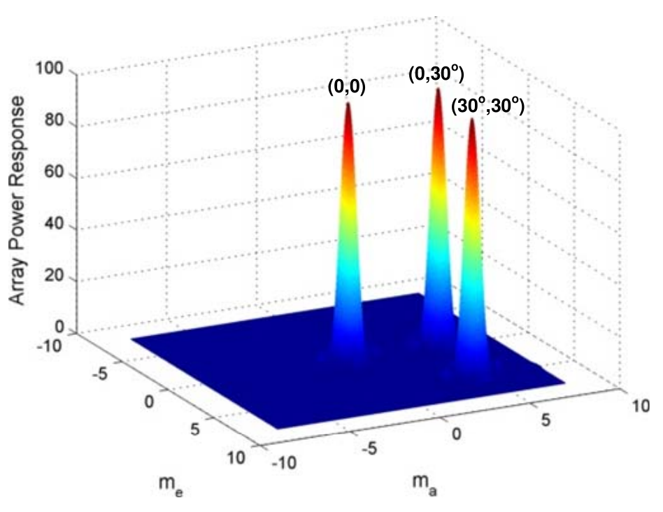
The array response in (4) is given by a product of two “sinc” functions that are related to the elevation and azimuth antenna/angle, respectively. Therefore, for any incident/departure signal from/to a particular direction , only those antennas located in the close vicinity of the focal point could receive/steer significant power; whereas the power of all other antennas located far away is almost negligible. As a result, any two simultaneously received/transmitted signals with sufficiently separated directions can be effectively discriminated over different antenna elements. This is illustrated by Fig. 2 which shows the power responses of the lens antenna array for three different signal directions . It is observed that the lens antenna array is able to separate signals both in elevation and azimuth directions, where their resolutions can be enhanced by increasing and , respectively, as can be inferred from (4). This general lens antenna array design is thus termed FD lens array. In the special case when the lens antenna array is designed by ignoring the signals’ elevation angles, the array response in (4) reduces to that studied in [25].
A prototype FD lens antenna array has been fabricated, based on which the preliminary measurement results have verified the angle-dependent energy focusing capabilities of FD lens arrays. The results are reported in [28].
II-B Multi-User Millimeter Wave Lens MIMO
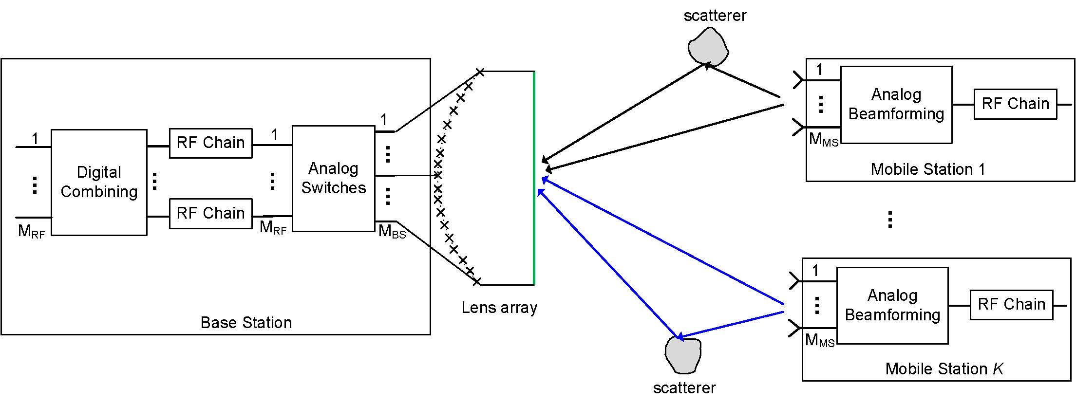
As shown in Fig. 3, we consider a single-cell uplink mmWave MIMO system with MSs served by a BS. The BS is equipped with an FD lens antenna array with antenna elements, and each of the MSs has a conventional antenna array such as UPA with elements. For cost-effective implementations, we assume that the BS has only RF chains, with , which are connected to the antennas with analog switches. Besides, each of the MSs is equipped with one RF chain only, which is connected to the antennas with analog phase shifters. Correspondingly, we assume that digital combining with antenna selection is performed at the BS receiver and analog beamforming is performed at the MS transmitters. Furthermore, we assume that the codebook-based analog beamforming is applied at the MSs, i.e., the analog beamforming vector of each MS is chosen from a pre-determined analog beamforming codebook , with denoting the codebook size and being the th analog beamformer with unit norm and all elements having identical amplitude. Note that codebook based analog beamforming has been commonly adopted for short-range mmWave systems [6], [10].
Under the general multi-path environment, the channel impulse response from MS to the th antenna of the BS can be modeled as
| (5) |
where is the -dimensional vector representing the channel coefficients from MS to BS antenna via path , with denotes the antenna set of the lens array at the BS, denotes the maximum number of channel paths which is typically small (e.g., no larger than 3) due to the multi-path sparsity of mmWave channels [3], and denote the complex-valued path gain and the delay for the th path, respectively, and are the elevation and azimuth AoA, respectively, and and are the elevation and azimuth AoD, respectively. Furthermore, is the lens array response at the BS as given in (4), and is the array response of the conventional array at the MS.
III Path Division Multiple Access
In this section, we assume perfect CSI at the BS as well as at the MSs, while the channel estimation scheme will be studied in Section IV. By exploiting the unique lens array response in (4), together with the multi-path sparsity of mmWave channels, we propose a PDMA scheme for multi-user mmWave lens MIMO systems that is applicable for the general wide-band frequency-selective channels. With this scheme, the MSs essentially communicate with the BS via distinct channel paths of different AoAs using the low-complexity SC transmission. As long as the lens array at the BS is sufficiently large to resolve all the multi-path signals from all MSs, PDMA is able to inherently eliminate both the ISI and IUI with only limited number of RF chains and low signal processing complexity.
With SC transmission, let be the independent information-bearing symbols sent by MS , with denoting the symbol index. The transmitted signal vector by the antennas of MS is given by
| (6) |
where denotes the transmit power of MS and is its analog beamforming vector chosen from the codebook . Note that only one data stream can be transmitted by each MS since it has only one RF chain.
Since only RF chains are available at the BS, antenna selection needs to be applied. Denote by with the subset of the selected BS antennas based on certain selection schemes (e.g., the low-complexity power-based antenna selection given in Section IV). Note that different from the conventional antenna systems, power-based antenna selection works particularly well for mmWave lens array, thanks to its energy focusing property. In particular, if , with denoting the maximum number of energy focusing antennas with non-negligible power for each path, then antenna selection at the BS incurs essentially no power loss. The signal received by the selected BS antennas can be expressed as
| (7) |
where denotes the discrete-time equivalent of the channel impulse response in (5), with denoting the path delay in symbol durations, and is the independent CSCG noise at the BS antenna with zero mean and power . Note that we assume the general wide-band channels such that , , . In the special case when certain paths of each user have identical delays (but different AoA/AoD without loss of generality), the following schemes can be directly applied by grouping those paths with identical delays.
It is observed from (7) that the received signal by each BS antenna is a superposition of the data streams, each arriving via multi-paths with different delays. In other words, (7) essentially constitutes a weighted linear combination of independent data symbols, where the weight of the th symbol is given by . As a consequence, the desired signal in for each MS in general suffers from both the ISI and IUI. However, a close look at the expression for reveals that, out of all the multi-paths, only those having the AoA with the energy focusing antenna around would have non-negligible signal contribution in , thanks to the “sinc” array response given in (4). This thus offers a unique opportunity for intrinsic ISI and IUI suppression, by equipping the BS with a sufficiently large lens antenna array with sufficiently fine angle resolution to resolve all the multi-paths. As a result, each MS may virtually communicate with the BS orthogonally via the non-overlapping energy focusing antennas corresponding to the different paths, thus termed PDMA.
For the generic systems where the BS is unable to perfectly resolve all the paths, we propose two PDMA receiver combining techniques for (7) based on MRC and MMSE, respectively. For ease of presentation, let be the set of all the paths. Furthermore, define
| (8) |
Physically, signifies the relative signal power received at BS antenna from path if all MSs transmit omni-directionally with identical power.
III-A MRC-based PDMA
With MRC-based PDMA, each BS antenna is synchronized to its strongest path, and the simple MRC receive combining is applied for detecting the signal from each MS based on the effective MIMO channel after applying a new technique called path delay compensation. Specifically, for , denote by the strongest path out of all the paths, i.e., and the set of the remaining paths. Then by synchronizing the receiver of BS antenna to path , in (7) can be decomposed as
| (9) |
where the second term in (9) consists of signals from all other paths at antenna , thus causes the inter-path interference (IPI), including both the ISI and IUI. With perfect path delay compensation at each antenna , i.e., by letting , (9) is equivalent to
| (10) |
where represents the IPI term in (9), and has the identical distribution as .
For each MS , let be the subset of the selected BS antennas that receive the strongest multi-path power from MS , i.e., . Note that if is too small, could be empty for those MSs that are far away from the BS and thus have weak channels. This is desirable from a sum-rate maximization perspective, but may cause the user fairness issue since the distant MSs may have very low or even zero data rate. Such an issue could be mitigated via proper user scheduling and/or power control, which is out of the scope of this paper. Since each antenna is associated with only one of the paths, we thus have , . For each MS , by concatenating , , as , (10) can be equivalently written as
| (11) |
where is the effective frequency-flat MIMO channel matrix after path delay compensation for MS with rows , , and denote the IPI and noise vector, respectively.
Denote by with the receive combining vector that is applied to (11) for detecting . With the MRC-based scheme, the IPI in (11) is not taken into account for the combiner design, and the transmit beamforming and receive combining vectors are designed to simply maximize the desired signal power for each MS , i.e.,
| (12) |
It can be shown that the optimal solution to (12) is
| (13) |
which can be obtained by comparing all the analog beamforming vectors in .
While the MRC-based design in (13) is sub-optimal in general due to the ignoring of the IPI term in (11), it is asymptotically optimal when and since in this case, the IPI term vanishes. Specifically, with , it is of high probability that each antenna receives non-negligible signal power from at most one path. As a result, , we have and hence . Thus, the IPI term in (9) vanishes, and (11) reduces to parallel frequency-flat small MIMO channels without any interference. Hence, maximizing the desired signal power as in (13) is optimal in this case.
The proposed MRC-based PDMA scheme with sufficiently separated AoAs is illustrated in Fig. 4 for the case of , and .
III-B MMSE-based PDMA
In this subsection, we propose the MMSE-based PDMA scheme with the ISI and IUI further mitigated. Under insufficient AoA separations, each antenna may potentially receive desired signal (as well as interference) for up to MSs. Thus, for detecting the data stream of each MS , all antennas should be utilized. Specifically, for detecting , antenna is synchronized to the strongest path, denoted as , among all the multi-paths of MS , where . With the received signal in (7) compensated by the corresponding delay by letting , the resultant signal for MS at antenna can be written as
| (14) |
where denotes the excessive path delay between the th path of MS and the th path of MS . Let denote the maximum path delay in symbol durations for all the paths, i.e., , . We then have . To derive the signal-to-interference-plus-noise ratio (SINR) expression for MS , the signals in (14) need to be reformulated by grouping those interfering symbols with identical excessive delays since they are correlated if originated from the same MS. To this end, for excessive delay , , and , we define
| (15) |
Then (14) can be equivalently written as
| (16) |
By concatenating the signals of all antennas in , (16) can be compactly written as
| (17) |
where is an vector with elements given by , , and with the rows given by , , is the effective MIMO channel matrix from MS to MS with excessive path delay . For detecting for MS , a receive combining vector with is applied to , which yields
| (18) |
By treating the ISI and the IUI as noise, the resultant SINR of MS can be expressed as (19) shown at the top of the next page,
| (19) |
where we have used the fact that the data symbols and are independent for or . As a result, an achievable data rate for MS is assuming Gaussian input, . The transmit and receive beamforming vectors can be optimized for sum-rate maximization by solving the following optimization problem
| (20) |
(P1) is a discrete optimization problem, which incurs an exponential complexity if the exhaustive search method is applied for finding the optimal solution.
We thus propose an efficient suboptimal solution to (P1) by firstly obtaining the best transmit beamforming vector by ignoring the ISI and IUI terms in (19), and then designing the receive combining vector with the interference properly mitigated. Specifically, by ignoring the ISI and IUI, is designed to maximize the numerator of (19) as
| (21) |
which can be obtained by comparing all analog beamformers in with complexity . With the transmit beamforming vectors fixed as in (21), the optimal receive combining vector to (P1) is given by the MMSE solution, i.e,
| (22) |
where
| (23) |
denotes the covariance matrix of the interference-plus-noise term for MS . The resultant SINR for MS is
| (24) |
IV Channel Estimation
In this section, we propose a novel channel estimation scheme tailored for the MRC-based PDMA scheme in single-sided lens MIMO system.11 1 The channel estimation scheme for the MMSE-based PDMA follows the same protocol as that for MRC-based PDMA, but is more complicated as more channel coefficients need to be estimated, which is thus omitted due to the space limitations. Note that for obtaining the complete knowledge of the channel impulse response of each MS , the BS in general needs to estimate the corresponding MIMO channel matrices for each of the taps, where denotes the maximum path delay in symbol durations. Furthermore, with only RF chains at the BS, it can be shown that such a brute-force channel estimation scheme requires a minimum training duration , which is prohibitive in practice. For example, for a typical system with (corresponding to and ), , , , and , we have . On the other hand, if the channel coherence time is ms, and the mmWave bandwidth is MHz, the total number of symbols within the channel coherence time is approximately . Thus, the required training duration with the brute-force training is even much longer than the channel coherence time, which is obviously impractical. In this section, by exploiting the angle and path sparsity of the mmWave channels jointly with the lens array enabled MRC-based PDMA scheme proposed in the preceding section, we propose an efficient channel estimation scheme with much reduced training overhead, which consists of three phases, namely power-based antenna selection, path estimation and association, and reduced MIMO channel estimation.
IV-A Power Based Antenna Selection at the BS
Since only RF chains are available at the BS, it needs to select antennas at the beginning of each channel coherence block. Thanks to the AoA-dependent energy focusing of lens antenna array as well as the limited number of multi-path for mmWave channels, it is intuitive that only those antennas located around the energy focusing regions of the multi-path signals should be selected, which can be attained based on the low-complexity power probing by the MSs. Specifically, in the first phase of channel estimation, the MSs simultaneously send identical power-probing symbols omni-directionally to the BS, i.e., , and , , where denotes the training duration of the first phase, represents the omni-directional analog beamformer applied by the MS with , . By discarding the first symbol durations during which not all multi-path signals have arrived, the received signal at BS antenna can be written as
| (25) |
where denotes the training power by each MS. Note that since identical power probing symbols are sent, i.e., , , the BS essentially receives the same signal across (without considering the noise). At the BS side, the RF chains sequentially scan over the antennas to obtain their respectively received power levels , . After that, those antennas with the highest power levels are selected, which are denoted by the set . Due to the “sinc”-type array response given in (4), it follows from (25) that those antennas in the vicinity of the energy focusing regions of the multi-paths are more likely to be selected, as desired. Furthermore, since the RF chain scanning process requires duration , the minimum required training duration for antenna selection in phase 1 can be obtained as .
IV-B Path Estimation and Association at the BS
The next training phase aims to associate each of the selected BS antennas with one of the paths (if any) for delay compensation and subsequent data reception. To this end, the relative strengths of the received signals via the different paths at antenna as well as their path delays are estimated. To avoid receiving the power training symbols sent in phase 1, a guard time of interval is inserted at the beginning of phase 2, as shown in Fig. 5. After that, each MS sends a pilot sequence , , with the omni-directional analog beamforming vector , where denotes the training duration of phase 2. The signal received by each of the selected BS antennas can be written as
| (26) |
where is defined in (8) signifying the relative path gain of path to BS antenna with omnidirectional transmission by the MSs. Based on the received signal in (26), the BS antenna needs to estimate the effective path gain as well as the path delay . To this end, (26) is reformulated in terms of all the taps. Specifically, since , , for tap delay , define
| (27) |
As a result, (26) can be equivalently written as
| (28) |
where , and . It is not difficult to see that estimating , , is sufficient for the estimation of both and for the paths. Note that (28) is equivalent to a MISO multi-path channel with taps, whose channel impulse response estimation has been extensively studied in the literature [30], [31]. To this end, (28) is compactly written as (29) shown at the top of the page,
| (29) |
where , , and . Based on the received training signal and the known pilots , the BS antenna can estimate using the least square (LS) estimation, i.e.,
| (30) |
In order to have a feasible estimation, the number of observations must be no smaller than the number of unknowns. Thus, we need . Based on the estimation , each BS antenna is associated with one path out of all the paths. For , let correspond to the strongest path arriving at BS antenna , i.e.,
| (31) |
where , , , are the elements of the estimated tap gains in . Then the desired path associated with BS antenna is set as
| (32) |
where is a certain threshold. In other words, the BS antenna is associated with the strongest path if the ratio of the received power from this path and that over all other paths is greater than a threshold ; otherwise, no path is associated with this antenna. Note that in the subsequent data transmission phase, if BS antenna is synchronized to path , then the signals received from all other paths will cause the detrimental ISI or IUI. Intuitively, the received signal by BS antenna would have non-negligible contribution for signal detection only if its received strongest path dominates over all other paths, i.e., the first case of (32) is true. Note that the path association rule in (32) is also applicable when antenna receives no significant power from any of the paths, in which case none of the path dominates and hence antenna will not be used for signal detection during the subsequent data transmission phase.
Note that with obtained, the corresponding path in terms of and the path delay can be obtained accordingly. Based on the above discussions, the minimum duration required for phase 2 is .
IV-C Reduced MIMO Channel Estimation
After phase 2 training, each of the selected BS antenna is associated with at most one desired signal path with its path delay estimated. Recall that is defined as the subset of the BS antennas that are associated with MS , i.e., . Then we have , . The objective of phase 3 training is to estimate the effective MIMO channel for each MS with its associated BS antennas in . At the beginning of phase 3 training, a guard time of duration is inserted to avoid receiving the training symbols sent in phase 2, as illustrated in Fig. 5. After that, each MS sends identical training symbol using a set of analog beamforming vectors that span the whole -dimensional space. Specifically, the -dimensional training signal vector sent by MS is
| (33) |
where is the training power, is the analog beamforming vector applied by the MSs at training duration , and is the minimum number of training duration in phase 3 for the analog beamformers to span the whole -dimensional space. Note that are chosen such that is a non-singular matrix.
For each MS , the signals received by its associated BS antennas can be written as
| (34) |
Note that for or . As the BS antenna has the knowledge of path delay of its associated path, it can apply the path delay compensation to by letting , which yields
| (35) |
where denotes the excessive path delay between path and . By concatenating for all , (35) can be compactly written as
| (36) |
where , and denote the concatenated ISI, IUI, and noise, respectively.
By further concatenating for all in (36), we have
| (37) |
where with rows given by , , is the effectively received training symbols by all the BS antennas associated with MS , with rows given by is the effective frequency-flat MIMO channel matrix from MS to its associated BS antennas after path delay compensation, and are the corresponding ISI, IUI, and noise matrix for MS . By treating ISI and IUI as noise, the effective MIMO channel matrix for MS can be estimated based on (37) with the LS estimation, i.e.,
| (38) |
Note that the effective MIMO channel estimation in (38) is in general subject to the ISI and IUI contaminations. However, based on the path association rule in (32), for each BS antenna that is associated with one MS, the ISI and IUI is dominated by the desired signal path, and hence their detrimental effect on channel estimation can be properly mitigated via choosing an appropriate threshold in (32). In particular, in the favorable scenario when all paths are well separated at the BS such that each BS antenna receives non-negligible power from at most one signal path, the ISI and IUI for channel estimation in (38) is negligible even for .
After obtaining the effective MIMO channel estimation for each MS , the BS obtains the optimized transmit and receive beamforming vectors based on (13) with replaced by . It then sends back the index of the analog beamforming vector to each MS . The total number of required feedback bits is .
Based on the previous discussions, the total time overhead required for phase 3 is . Thus, the total time required for the proposed channel estimation scheme is , which is much smaller than as required by the brute force channel impulse response estimation. For the example given at the beginning of this section, we have . Besides, as compared to the channel coherence time , the time overhead of the proposed channel estimation scheme is and thus negligible.
The frame structure of the proposed channel estimation scheme is illustrated in Fig. 5.
V Simulation Results
In this section, simulation results are provided to compare the performance of the proposed lens-based system with that based on the conventional antenna arrays. For both systems, we assume that each MS is equipped with the conventional UPA with elements, whereas the BS either has a FD lens array (proposed), or a UPA (benchmark) with adjacent elements separated by half wavelength. We assume that both the lens array and the UPA at the BS have the same effective aperture , and the lens array is designed to have the maximum coverage angles . Thus, the total number of BS antennas for UPA is and that for the lens array can be obtained as . We assume that the system operates at GHz and the mmWave channel for each MS has paths, with the azimuth and elevation angles independently and uniformly distributed in . Furthermore, the path delays are uniformly distributed in , with ns denoting the maximum path delay. We assume that all MSs are m away from the BS, and the path loss and power division among different multi-paths are generated based on the model developed in [32]. We further assume that the total available bandwidth is MHz. As a result, we have , so that the system is wide-band and frequency-selective in general. For the benchmark UPA system, we assume that perfect CSI is available at the BS and MSs and MIMO-OFDM transmission is adopted, with sub-carriers and cyclic prefix (CP) symbols. To cater for the limited number of RF chains at the BS side, the approximate Gram-Schmidt based hybrid analog/digital signal processing scheme for MIMO-OFDM proposed in [17] is applied for the UPA system. On the other hand, for the lens system, we consider both cases with perfect CSI as well as the estimated CSI as proposed in Section IV, where the threshold in (32) for channel estimation is set to zero. After the power-based antenna selection in the lens system, we employ the proposed MRC-based (for both perfect and estimated CSI) and MMSE-based (for perfect CSI only) PDMA schemes, which only require the low-complexity SC transmission and path delay compensation at the BS. At the MS side, we assume that both the UPA and lens systems apply analog beamforming with the beamsteering codebook of size , which is obtained by uniformly quantizing the azimuth and elevation angles. Note that to account for the training overhead of the proposed channel estimation scheme, we assume that the channels are quasi-static that remain unchanged for ms, or equivalently about symbols for SC transmission with bandwidth MHz. Thus, the training overhead can be calculated based on Section IV for different number of RF chains, .

V-A Single-User System
First, we consider the special case of single-user system with , for which the hybrid processing scheme proposed in [17] can be directly applied. By assuming that the BS has RF chains, Fig. 6 shows the spectrum efficiency versus the SNR of the data transmission phase for various schemes. It is observed that for the lens system with perfect CSI, the proposed MRC- and MMSE-based schemes achieve almost identical performance. This is expected since in the single-user setup with a total of three paths only, all multi-path signals are well separated at the BS almost surely and thus the IPI (or equivalently ISI in this case) vanishes. Furthermore, by setting the training SNR as 10dB, it is found that the performance of the MRC-based scheme with the estimated CSI is very close to that based on perfect CSI, which shows the efficacy of the channel estimation scheme proposed in Section IV. Note that for the setup under consideration, the required training length for each channel coherent block can be calculated as 373, which is only about 0.75% of the channel block length and hence is negligible. Moreover, it is noted from Fig. 6 that even with estimated CSI, the proposed lens system achieves higher spectrum efficiency than the benchmark UPA system based on perfect CSI, which requires the more sophisticated MIMO-OFDM and hybrid signal processing schemes. The performance gain is mainly attributed to the saving of the CP overhead with the proposed lens-based design, the efficacy of the proposed channel estimation scheme with almost negligible training overhead, as well as the effective ISI mitigation and coherent signal combining after path delay compensation at the BS.

Fig. 7 shows the achievable spectrum efficiency versus the number of RF chains at the BS, where the SNR for the data transmission phase is set as dB. It is observed that for all the schemes, the performance in general enhances as more RF chains are available at the BS, but only marginal improvement is observed as exceeds . In particular, for all the schemes under consideration, by equipping the BS with only RF chains is able to achieve over of the spectrum efficiency as compared to the full RF chain case. This is expected since as increases, the system performance will be eventually constrained by the limited number of signal paths of the mmWave channels.

V-B Multi-User System
Next, we consider the multi-user system with MSs. Since, to the best of the authors’ knowledge, no hybrid processing designs were reported for the multi-user wide-band MIMO-OFDM systems, the benchmark scheme is simply chosen to be the hybrid scheme proposed in [17] for single-user MIMO-OFDM system together with time division multiple access (TDMA), i.e., each of the MSs is served by the BS for of the time. Fig. 8 shows the achievable spectrum efficiency for different schemes by assuming the BS has RF chains. It is observed that for the lens MIMO system, the MMSE- and MRC-based PDMA schemes have almost identical performance in the low-SNR regime, whereas the performance gap increases as the SNR increases. This is expected since for multi-user setup with more signal paths in total, the IPI becomes stronger as the SNR increases. Furthermore, by setting the training SNR as dB, it is found that the proposed channel estimation scheme results in comparable performance as the perfect CSI case, which shows its effectiveness for multi-user system as well. Fig. 8 also shows that the proposed lens system significantly outperforms the UPA system, mainly due to the more efficient multiple-access scheme (PDMA) compared to TDMA. However, even by ignoring the time division loss of TDMA (via multiplying the sum-rate by a factor of ) and thus obtaining a (loose) performance upper bound for the UPA-based hybrid system, the proposed lens system still performs comparably well for all SNRs.

Fig. 9 shows the achievable spectrum efficiency for the multi-user system versus the number of RF chains at the BS, where the SNR for data transmission is set as dB. Similar to the single-user case, the spectrum efficiency of the lens-based scheme for multi-user systems increases with . In particular, with only RF chains at the BS, about of the spectrum efficiency achievable by the full RF chain system can be attained. Fig. 9 also shows that as increases, there is no evident performance improvement for the benchmark UPA system, since at each instance the BS only serves one MS with a single data stream due to the use of TDMA.
VI Conclusion
This paper studies the uplink multi-user mmWave MIMO communication with single-sided FD lens antenna array at the BS and conventional UPA at each MS. Under limited RF chains at the BS and one single RF chain at each MS, we first propose an efficient PDMA scheme, by which each MS essentially communicates with the BS via different channel paths with the low-complexity SC transmission and path delay compensation at the BS. For general scenarios with insufficiently separated AoAs, analog beamforming at the MSs is jointly designed with digital combining at the BS based on MRC and MMSE, respectively. Furthermore, we propose an efficient channel estimation scheme tailored for the MRC-based PDMA scheme, which incurs almost negligible training overhead in practical mmWave systems and yields comparable performance as the case with perfect CSI. Numerical results are provided to show the sum-rate gain of the proposed design over the benchmark UPA systems based on MIMO-OFDM and hybrid analog/digital signal processing at the BS, which in general require higher signal processing complexity and hardware/energy costs than the proposed system.
Appendix A Proof of Lemma 1
The proof of the array response in (4) extends that in Appendix A of [25] by considering the signals’ elevation angles. We will assume that the lens array is used for signal reception, and the proof of transmit array response can be obtained similarly due to reciprocity. Let denote the physical dimension of the EM lens, and with denote its phase shift profile, which represents the phase delay provided by the spatial phase shifters (SPS) at each point on the lens’s aperture. Further denote by with coordinate the focal point of the lens for normal incident plane waves, where is the focal length. To ensure constructive superpositions at for all rays with normal incidence, must be designed to be [25]
| (39) |
where denotes the common phase shift from the lens’s input aperture to the focal point , and is the wave number corresponding to the signal wavelength . With designed as in (39), the resulting phase delay from the lens’s input aperture to antenna with coordinate can be expressed as
| (40) |
where denotes the distance from the point on the lens to antenna , and (40) follows from the first-order Taylor approximation with the assumption .
Denote by the arriving signal at point of the lens’s input aperture. Due to the linear superposition principle, the resultant signal at antenna can then be expressed as
| (41) |
For a uniform incident plane wave with elevation AoA and azimuth AoA , the arriving on the lens aperture can be expressed as
| (42) |
where is the input signal arriving at the reference point (chosen as the lens center) of the lens, and is a normalization factor to ensure that the total power captured by the lens is proportional to its effective aperture . By substituting (42) and (40) into (41), can be written as (43) shown at the top of the next page,
| (43) |
where we have used the identity and . By substituting (1) and (2) into (43) and with the definition , the array response in (4) can be obtained.
This completes the proof of Lemma 1.
References
- [1] Z. Pi and F. Khan, “An introduction to millimeter-wave mobile broadband systems,” IEEE Commun. Mag., vol. 49, no. 6, pp. 101–107, Jun. 2011.
- [2] T. S. Rappaport, et al., “Millimeter wave mobile communications for 5G cellular: it will work!” IEEE Access, vol. 1, pp. 335–349, May 2013.
- [3] T. S. Rappaport, R. W. Heath Jr, R. C. Daniels, and J. N. Murdock, Millimeter Wave Wireless Communications. Prentice Hall, 2014.
- [4] W. Roh, et al., “Millimeter-wave beamforming as an enabling technology for 5G cellular communications: theoretical feasibility and prototype results,” IEEE Commun. Mag., vol. 52, no. 2, pp. 106–113, Feb. 2014.
- [5] P. Wang, Y. Li, L. Song, and B. Vucetic, “Multi-gigabit millimeter wave wireless communications for 5G: From fixed access to cellular networks,” IEEE Commun. Mag., vol. 53, no. 1, pp. 168–178, Jan. 2015.
- [6] T. Baykas, et al., “IEEE 802.15.3c: the first IEEE wireless standard for data rates over 1Gb/s,” IEEE Commun. Mag., vol. 49, no. 7, pp. 114–121, Jul. 2011.
- [7] T. Nitsche, et al., “IEEE 802.11ad: directional 60 GHz communication for multi-Gigabit-per-second Wi-Fi,” IEEE Commun. Mag., vol. 52, no. 12, pp. 132–141, Dec. 2014.
- [8] Https://www.fcc.gov/document/fcc-adopts-rules-facilitate-next-generation-wireless-technologies.
- [9] S. Rangan, T. S. Rappaport, and E. Erkip, “Millimeter-wave cellular wireless networks: potentials and challenges,” Proceedings of the IEEE, vol. 102, no. 3, pp. 366–385, Mar. 2014.
- [10] J. Wang, et al., “Beam codebook based beamforming protocol for multi-gbps millimeter-wave WPAN systems,” IEEE J. Sel. Areas Commun., vol. 27, no. 8, pp. 1390–1399, Oct. 2009.
- [11] F. Gholam, J. Via, and I. Santamaria, “Beamforming design for simplified analog antenna combining architectures,” IEEE Trans. Veh. Technol., vol. 60, no. 5, pp. 2373–2378, Jun. 2011.
- [12] S. Hur, et al., “Millimeter wave beamforming for wireless backhaul and access in small cell networks,” IEEE Trans. Commun., vol. 61, no. 10, pp. 4391–4403, Oct. 2013.
- [13] X. Zhang, A. F. Molish, and S. Y. Kung, “Variable-phase-shift-based RF-baseband codesign for MIMO antenna selection,” IEEE Trans. Signal Process., vol. 53, no. 11, pp. 4091–4103, Nov. 2005.
- [14] V. Venkateswaran and A. J. van der Veen, “Analog beamforming in MIMO communications with phase shift networks and online channel estimation,” IEEE Trans. Signal Process., vol. 58, no. 8, pp. 4131–4143, Aug. 2010.
- [15] O. E. Ayach, S. Rajagopal, S. Abu-Surra, Z. Pi, and R. W. Heath Jr, “Spatially sparse precoding in millimeter wave MIMO systems,” IEEE Trans. Wireless Commun., vol. 13, no. 3, pp. 1499–1513, Mar. 2013.
- [16] A. Alkhateeb, G. Leus, and R. W. Heath Jr, “Limited feedback hybrid precoding for multi-user millimeter wave systems,” IEEE Trans. Wireless Commun., vol. 14, no. 11, pp. 6481–6494, Nov. 2015.
- [17] A. Alkhateeb and R. W. Heath, “Frequency selective hybrid precoding for limited feedback millimeter wave systems,” IEEE Trans. Commun., vol. 64, no. 5, pp. 1801–1818, May 2016.
- [18] F. Sohrabi and W. Yu, “Hybrid digital and analog beamforming design for large-scale antenna arrays,” IEEE J. Sel. Topics Signal Process., vol. 10, no. 3, pp. 501–513, Apr. 2016.
- [19] A. Alkhateeb, O. E. Ayach, R. Leus, and R. W. Heath Jr, “Channel estimation and hybrid precoding for millimeter wave cellular systems,” IEEE J. Sel. Topics Signal Process., vol. 8, no. 5, pp. 831–846, Oct. 2014.
- [20] Z. Gao, C. Hu, L. Dai, and Z. Wang, “Channel estimation for millimeter-wave massive MIMO with hybrid precoding over frequency-selective fading channels,” IEEE Commun. Letters, vol. 20, no. 6, pp. 1259–1262, Jun. 2016.
- [21] J. Singh, O. Dabeer, and U. Madhow, “On the limits of communication with low-precision analog-to-digital conversion at the receiver,” IEEE Trans. Commun., vol. 57, no. 12, pp. 3629–3639, Dec. 2009.
- [22] A. Artemenko, et al., “Millimeter-wave electronically steerable integrated lens antennas for WLAN/WPAN applications,” IEEE Trans. Antennas Propag., vol. 61, no. 4, pp. 1665–1671, Apr. 2013.
- [23] J. Brady, N. Behdad, and A. M. Sayeed, “Beamspace MIMO for millimeter-wave communications: system architecture, modeling, analysis, and measurements,” IEEE Trans. Antennas Propag., vol. 61, no. 7, pp. 3814–3827, Jul. 2013.
- [24] Y. Zeng, R. Zhang, and Z.-N. Chen, “Electromagnetic lens-focusing antenna enabled massive MIMO: performance improvement and cost reduction,” IEEE J. Sel. Areas Commun., vol. 32, no. 6, pp. 1194–1206, Jun. 2014.
- [25] Y. Zeng and R. Zhang, “Millimeter wave MIMO with lens antenna array: a new path division multiplexing paradigm,” IEEE Trans. Commun., vol. 64, no. 4, pp. 1557–1571, Apr. 2016.
- [26] T. Kwon, Y.-G. Lim, B.-W. Min, and C.-B. Chae, “RF lens-embedded massive MIMO systems: fabrication issues and codebook design,” IEEE Trans. Microw. Theory Techn., vol. 64, no. 7, pp. 2256–2271, Jul. 2016.
- [27] L. Yang, Y. Zeng, and R. Zhang, “Efficient channel estimation for millimeter wave MIMO with limited RF chains,” in Proc. IEEE Int. Conf. Commun., May 22-27, 2016.
- [28] Y. Zeng and R. Zhang, “Cost-effective millimeter wave communications with lens antenna array,” submitted for publication, available online at https://arxiv.org/abs/1610.02511.
- [29] L. Dai, X. Gao, S. Han, C. Lin, and X. Wang, “Beamspace channel estimation for millimeter-wave massive MIMO systems with lens antenna array,” in Proc. IEEE Int. Conf. Commun. China (ICCC), Jul. 2016.
- [30] H. Vikalo, B. Hassibi, B. Hochwald, and T. Kailath, “On the capacity of frequency-selective channels in training-based transmission schemes,” IEEE Trans. Signal Process., vol. 52, no. 9, pp. 2572–2583, Sep. 2004.
- [31] X. Ma, L. Yang, and G. B. Giannakis, “Optimal training for MIMO frequency-selective fading channels,” IEEE Trans. Wireless Commun., vol. 4, no. 2, pp. 453–466, Mar. 2005.
- [32] M. R. Akdeniz, et al., “Millimeter wave channel modeling and cellular capacity evalutation,” IEEE J. Sel. Areas Commun., vol. 32, no. 6, pp. 1164–1179, Jun. 2014.