Proposal for quantum many-body simulation and torsional matter-wave interferometry with a levitated nanodiamond

Micro and Nano-mechanical resonators in the quantum regime, based on light-matter interaction, have wide applications in quantum metrology and quantum information science [1]. It is one of the best test-beds for generating macroscopic quantum superpositions, and studying quantum-classical boundaries [2, 3]. To this end, mechanical resonators need to be coupled to other systems, such as atoms [4], superconducting circuits [5, 6], cavity modes [1], nitrogen-vacancy (NV) centers [7, 8, 9], etc. Among these systems, NV centers attract a great attention [10] due to the extraordinary long coherence time (ms) even at room temperature[11] as well as its high manipulation and detection efficiency. The center-of-mass motion can even be coupled to the electron spins in magnetic field with a large gradient[7, 17]; typically this gradient should be of the order of $10^{7}$ T/m, which is difficult to achieve in stat-of-art experiments. Furthermore, this large magnetic gradient prevents collective coupling between NV electron spin ensemble and the mechanical oscillator.

The motion of the nanoparticles can behave in a totally different way when levitated in a high quality vacuum by optical trapping[18, 20, 19]. In this case the nanoparticles can vibrate along different directions controlled by the external optical field. In recent years this torsional vibration for a nonspherical nanodiamond in an optical trap in vacuum was observed[21]. It was also proposed that a torsional mode can be cooled down to the ground state by a linearly polarized cavity mode [21, 22]. In this work, we investigate the coupling between the torsional vibration of a levitated nanodiamond and NV center electron spins (see Fig. 1). The orientation of an NV center will change together with the torsional vibration of the nanodiamond [23], thus even in a uniform magnetic field the energy levels of the NV electron spins can still depend strongly on its orientation as well as its displacement from the origin, which induce coupling between the torsional vibration and the NV spin. We find that strong coupling can be reached with a modest uniform magnetic field (for example $0.05$ T), thus can circumvent the technical difficulty mentioned above[7, 17].

We also propose several applications of spin-torsional coupling. We show how to realize matter-wave interferometry, and propose to use the collective coupling between an ensemble of NV electron spins and the torsional mode to realize the Lipkin-Meshkov-Glick (LMG) model [24, 25, 26]. The LMG model was first introduced in nuclei physics for phase transitions, and has been found to be relevant to a large number of quantum systems such as Bose-Einstein condensates in different traps [27, 28, 29, 30], the Bardeen-Cooper-Schrieffer superconducting model [31], the radiation-matter Dicke model [32, 33, 34, 35] and cavity QED [36]. Up to now the special case of LMG model was realized [37, 38] in ultracold atoms and the corresponding transition from Rabi dynamics to Josephson dynamics has been reported, yet the full LMG model has never been experimentally realized. We show that the quantum phase transition in the LMG model and finite number effects can be observed in our proposed system.

We consider a non-spherical nanodiamond with one long axis and two short axes optically trapped in high vacuum [21, 39] in a static uniform magnetic field (Fig. 1). The direction of the nanodiamond can be manipulated and aligned with the laser field [21, 40, 23]. We consider the torsional vibration of the nanodiamond along $\theta$ direction around the polarization direction of the laser beam. The torsional Hamiltonian is $H_{tor}=\omega_{\theta}b^{\dagger}b$ (with natural unit $\hbar=1$). Typically $\omega_{\theta}$ is of the order of MHz.

We first consider a single NV center in the nanodiamond. The direction of the magnetic field is denoted as $z$ while the intrinsic quantization direction of the NV center is denoted as $z^{\prime}$ (see Fig 1). The Hamiltonian of the NV center is $H_{NV}=DS_{z^{\prime}}^{2}+g\mu_{B}{\mathbf{B}}\cdot{\mathbf{S}}$, where $D=2.8$ GHz for typical NV center. $S_{z(z^{\prime})}$ is the spin-1 operator along $z(z^{\prime})$ direction. If we use the eigenvectors of $S_{z^{\prime}}$ to expand $H_{NV}$, and define $\Delta=-g\mu_{B}|{\mathbf{B}}|$, the Hamiltonian becomes [41]

If the gradient of $\mathbf{B}$ is large, the strong coupling between the translational motion of the diamond and the spin $\mathbf{S}$ could be achieved [17, 9].

Here we suppose that $\mathbf{B}$ is homogeneous, and $\theta$ changes with the torsional motion. The angles $\theta_{0}$ and $\phi_{0}$ denote the equilibrium orientation. The eigenvalues for $H_{NV}$ is determined by the following cubic function,

which is independent of phase $\phi$. The calculated eigenvalues $z=E_{i}$ ($i=-1,0,1$) for a modest magnetic field as a typical example is shown in Fig 2(a). We only deal with two spin states, $|S_{z^{\prime\prime}}=-1\rangle$ and $|S_{z^{\prime\prime}}=0\rangle$, where $S_{z^{\prime\prime}}$ is the spin operator in whose representation $H_{NV}(\theta_{0},\phi_{0})$ is diagonal. We change the energy zero point to $E_{0}$ and define the energy of $|S_{z^{\prime\prime}}=-1\rangle$ as $E(\theta,\phi)=E(\theta)=E_{-1}(\theta)-E_{0}(\theta)$.

The total Hamiltonian for the NV center and the torsional oscillator reads

where $\sigma_{z^{\prime\prime}}=|S_{z^{\prime\prime}}=-1\rangle\langle S_{z^{\prime\prime}}=-1|-|S_{z^{\prime\prime}}=0\rangle\langle S_{z^{\prime\prime}}=0|$. We let $|S_{z^{\prime\prime}}=-1\rangle\equiv|-1\rangle$ and $|S_{z^{\prime\prime}}=0\rangle\equiv|0\rangle$. This is the representation that we will focus on in the rest of this paper. The coupling between the torsional mode and NV center electron spin is

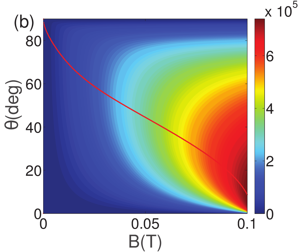
where $I$ is the moment of inertia, and $\omega_{\theta}$ is the angular frequency of the torsional mode [21]. As shown in Fig. 2(b), $g_{N}/2\pi$ could be about $300$ kHz at $0.05$ T, which is much larger than both torsional mode decay ($<$ kHz) [21] and the NV center decay ($<$ kHz ) and dephasing ($\sim$ kHz) rates [42]. Therefore the strong coupling condition is fulfilled. In experiments the value of $g_{N}$ can be tuned in a wide range by controlling either the trap potential or the external uniform magnetic field. The typical energy scales used in this paper are summarized in Table 1.

Here we show that this novel platform provides an excellent opportunity to simulate the LMG model[24, 25, 26]. For the nanodiamond considered here, the mean separation between NV centers is assume to be $d>15$ nm and the direct dipole-dipole interactions between NV centers ($J_{\text{d-d}}<20$ kHz [44]) are much smaller than the spin-torsional coupling ($\sim 300$ kHz at 0.05 T). The coherence time of NV centers in nanodiamond at such low concentration could be around ms [11, 42, 43]. As multiple NV centers are coupled to the same torsional mode coherently in a uniform magnetic field, the torsional mode mediating coupling between NV centers can be strong using a proper experimental scheme. To realize the LMG model, a microwave driving field with frequency $\omega_{l}$ and Rabi frequency $\Omega$ is added. The Hamiltonian of the system that contains multiple NV centers and the microwave drive is,

where $S_{\alpha}=\sum_{j=1}^{N}\sigma_{\alpha}^{j}$ for $\alpha=x^{\prime\prime}$, $y^{\prime\prime}$ and $z^{\prime\prime}$ are the total spin operators for a system with $N$ NV centers in $z^{\prime}$ direction. $S^{+}=(S_{x^{\prime\prime}}+iS_{y^{\prime\prime}})/2$ and $S^{-}=(S_{x^{\prime\prime}}-iS_{y^{\prime\prime}})/2$. NV centers along other directions (see Fig 1) can be neglected as they have very different energy levels. In our model, the torsional mode mediated spin flip is forbidden in the $x^{\prime\prime}-y^{\prime\prime}-z^{\prime\prime}$ coordinate. Thus the last driving term should be included to realize the long-range LMG model. The above time-dependent model, in which $E_{0}$ and $\omega_{l}$ are the dominante frequencies, can be transformed to the low-frequency stationary Hamiltonian $H_{\text{eff}}=U^{\dagger}HU-U^{\dagger}i\partial_{t}U$ via a unitary rotation $U=e^{-i\omega_{l}tS_{z^{\prime\prime}}/2}$. We obtain

where $E_{0}^{\prime}=E_{0}-\omega_{l}$. So the microwave driving field only affects the effective Zeeman field along the $z^{\prime\prime}$ direction. We suppose resonant driving condition fulfilled with $E_{0}^{\prime}=0$, in which case an isotropic LMG model can be realized.

To adiabatically eliminate the influence of the torsional mode, we need to go into a rotating frame. Let us define $H_{\text{eff}}=H_{0}+V$. Here $H_{0}=\omega_{\theta}b^{\dagger}b+\frac{\Omega_{0}}{2}S_{x^{\prime\prime}}$ defines which rotating frame we use, where $\Omega_{0}$ is the frequency of the rotating frame for NV centers. In an experiment, it could be adjusted by changing the frequency of a local reference oscillator. $V$ is treated as perturbation, which is a quite good approximation regarding that $\Omega\sim\Omega_{0}\sim\omega_{\theta}$ is the leading term in Eq. (6), while all the other coefficients are much smaller than these energy scales (see Table 1). After the transformation the Hamiltonian $H_{\text{eff}}$ is represented by the interaction term

where $\tilde{S}_{+}=(\tilde{S}_{x}+i\tilde{S}_{y})/2$, $\tilde{S}^{-}=(\tilde{S}_{x}-i\tilde{S}_{y})/2$ and $h_{0}=\Omega-\Omega_{0}$. Notice that here we have adopted the notations: $S_{x^{\prime\prime}}=\tilde{S}_{z}$, $S_{y^{\prime\prime}}=-\tilde{S}_{y}$, and $S_{z^{\prime\prime}}=\tilde{S}_{x}$.

Here we consider many NV centers in a single nanodiamond. The single spin-torsional coupling strength $g_{N}\propto 1/\sqrt{I\omega_{\theta}}$ depends on the torsional frequency $\omega_{\theta}$ and the size of the nanodiamond. We suppose the concentration of NV center is kept as a constant. As the size of nanodiamond increases, both $I$ and $N$ will increase. However, the coupling strength $g_{N}$ decreases. We suppose that $g_{N}\propto 1/\sqrt{N}$. In the following discussion, we define $g=\sqrt{N}g_{N}$ as the collective spin-torsional coupling strength. The effective Hamiltonian can be derived using the method in Refs. [45, 46, 47]. In the limit that $\Omega_{0}\pm\omega_{\theta}\gg g_{N},h_{0}$, we get

where $\lambda=\frac{g^{2}}{8}\cdot\frac{\omega_{\theta}}{\Omega_{0}^{2}-\omega_{\theta}^{2}}$, $h=\frac{h_{0}}{2}+\frac{\Omega_{0}}{\Omega_{0}^{2}-\omega_{\theta}^{2}}\cdot(b^{\dagger}b+\frac{1}{2}){g^{2}/2N}$.

We mainly focus on the condition of ferromagnetic coupling ($\lambda<0$) when $\omega_{\theta}>\Omega_{0}$. The effective Zeeman field is consisted of two parts: the contribution from the external Zeeman field inherent from the original Hamiltonian and the contribution from phonons. Notice that the second part is due to the fact that the interaction $V_{\text{int}}$ breaks the time-reversal symmetry. This term will become unimportant if the total number of NV centers $N$ is large enough. The first term $h_{0}$ will play primary role for the phase transition near torsional ground state or when $N$ is much larger than the torsional thermal phonon number $\langle b^{\dagger}b\rangle$. For $h\ll\Omega_{0}$ the change of $h$ will not significantly change the coupling strength $\lambda$, thus these two parameters may be treated as independent parameters. In the above calculations, we focused on the resonant excitation ($E_{0}^{\prime}=0$). Thus the two orthogonal directions ($x$ and $y$) are equivalent. When $E_{0}^{\prime}\neq 0$, the equivalence between these two directions is broken and the asymmetric LMG model may also be realized. If there is no driving field, the spin-flipping is forbidden thus only long-range classical Ising model can be realized [48], which may also support phase transition belonging to a totally different universal class due to the fact that a $d$ (here $d=1$) dimensional quantum spin model is equivalent to the $(d+1)$ dimensional classical model. This system also has the potential to study antiferromagnetism [49].

In the thermodynamic limit, the LMG model hosts phase transition at $h=\lambda$. In realistic systems, the number of NV centers in a diamond nanocrystal is always finite and can be controlled by doping. For a 80 nm-diameter diamond, the total number of NV color centers can be in the range of $N\sim 0-100$, which is sufficient to observe the phase transitions [50, 51]. In this model the order parameters are defined as $m_{xy}=\frac{2}{N}\sqrt{\langle\tilde{S}_{x}^{2}+\tilde{S}_{y}^{2}\rangle}$ for the in-plane polarization, and $m_{z}=\frac{2}{N}\sqrt{\langle\tilde{S}_{z}^{2}\rangle}$ for the out-of-plane polarization[54, 52, 53]. For a finite system, we find $m_{z}=1$ when $|h/\lambda|\geq 1$, and otherwise,

where $[x]$ takes the integer part of $x$. The in-plane polarization can be determined via $m_{xy}=\sqrt{1+\frac{2}{N}-m_{z}^{2}}$. We see that the discontinuous jump of $m_{z}$ and $m_{xy}$ can be observed at $\frac{h}{\lambda}=\frac{2k}{N}$ for $k=1,2,3,\cdots,[\frac{N}{2}]$ when $N$ is odd and $\frac{h}{\lambda}=\frac{2k-1}{N}$ for $k=1,2,3,\cdots,[\frac{N}{2}]$ when $N$ is even. The jump of these quantities arises from the quantization of the spin. These two polylines will collapse to the well-known continue limit, $m_{xy}=\sqrt{1-(h/\lambda)^{2}}$ and $m_{z}=\frac{h}{\lambda}$ for $|h/\lambda|<1$, when $N\rightarrow\infty$.

Both analytical results and numerical results for $m_{xy}$ and $m_{z}$ (see Fig. 3) suggest that the strong signature of quantum phase transition can be observed even in a small system. When $|h/\lambda|>1$, the out-of-plane polarization $m_{z}$ exactly equals to one, while the in-polarization can still be finite ($m_{xy}=\sqrt{\frac{2}{N}}\approx 0.3$ when $N=18$). This is different from the proposal for classical phase transition in Ref. 48, where an experimentally observable effect requires an extraordinary large number of NV centers.

To observe the phase transition, we can measure $m_{z}$ as a function of $h/\lambda$. We prepare the NV centers in ground state, then adiabatically tune the parameter $h/\lambda$. The exact degeneracy at the jumping point should be removed by a modest in-plane Zeeman field. Experimentally, we measure the population of the spin in the intrinsic quantization direction $z^{\prime}$. We can first apply a microwave pulse that rotates the state $\tilde{S}_{z}$ to the state $S_{z^{\prime}}$, and then measure the spin state in the intrinsic frame.

Schrödinger’s cat state is generally considered as an entangled state between a microscopic quantum system and a macroscopic system. It can be prepared with an optically levitated nanodiamond using the coupling between the center-of-mass motion and the electron spin with a strong magnetic gradient  [17]. Here we show how to realize Schrödinger’s cat state with torsional motion and spin in a uniform magnetic field.

First we need to cool the torsional motion near ground state $|0\rangle_{\theta}$ by sideband cooling [21, 55, 56]. Then we adiabatically lower the trapping frequency from $\omega_{\theta}$ to $\omega_{\theta}^{\prime}$ so that $|0\rangle_{\omega_{\theta}}$ evolves to a new vacuum state $|0\rangle_{\omega_{\theta}^{\prime}}$. The spin is initialized to $(|0\rangle+|-1\rangle)/\sqrt{2}$. From $t=0$, the system evolves under the Hamiltonian (3) where $\omega_{\theta}$ is replaced by $\omega_{\theta}^{\prime}$. We find that the system splits into two torsional oscillations centered at slightly different orientations and coupled with the two spin states respectively (see appendix A). At time $t_{0}=\pi/\omega_{\theta}^{\prime}$, the separation of orientation is the largest. The state at this time is

which is the Schrödinger’s cat state. For convenience we define $\beta=g_{N}/\omega_{\theta}^{\prime}$. With the displacement operator $\hat{D}(\beta)=\exp(\beta b^{\dagger}-\beta^{*}b)$, we get $\hat{D}(\beta)|0\rangle_{\omega_{\theta}^{\prime}}=|\beta\rangle_{\omega_{\theta}^{\prime}}$, and $\hat{D}(-\beta)|0\rangle_{\omega_{\theta}^{\prime}}=|-\beta\rangle_{\omega_{\theta}^{\prime}}$.

We can use matter-wave interferometry to verify the creation of the Schrödinger’s cat state. First, we impose pulses to disentangle the spin and the oscillation [17]. The torsional motion state becomes $|\varphi^{\prime}(t_{0})\rangle=\frac{1}{\sqrt{2}}(|\beta\rangle_{\omega_{\theta}^{\prime}}+|-\beta\rangle_{\omega_{\theta}^{\prime}})$. Then we turn off the magnetic field and the optical tweezer. The spin state $|0\rangle$ tends to rotate to the lowest energy state adiabatically similar as the trend in Fig. 2(a) under the influence of the earth magnetic field. Its timescale is larger than $0.1\ \rm{s}$, slow enough to be neglected. Suppose $zn$ is the direction perpendicular to $oz$ and $oz^{\prime}$ in Fig. 1(a). The Hamiltonian for the system is $H_{free}=L_{zn}^{2}/2I$, where $L_{zn}$ is the orbital angular momentum operator along $zn$. The orientation of the nanodiamond evolves freely and creates an interference pattern in $\theta$ direction (see appendix B).

Fig. 4 shows examples of the calculated interference fringe. When the evolutionary time is not very long, the longer the time is, the wider the fringe will be. But when the time is too long, the wavefunction spreads over a full $2\pi$ angle, the interference fringe becomes very complex. We only need to focus on the region without the complicate pattern.

We discuss the strong coupling mechanism between the torsional motion of a nanodiamond and the spin of built-in NV centers under a homogeneous magnetic field. This novel system can used for simulating LMG model and the many-body phase transitions. Strong evidence for this phase transition can even be observed for a small nanodiamond containing only a few tens of NV centers. The system may also be used to realize Schrödinger cat state and the corresponding torsional matter-wave interferometry.

References

- [1] M. Aspelmeyer, T. J. Kippenberg, and F. Marquardt, Reviews of Modern Physics 86, 1391 (2014).
- [2] M. Poot and H. S. J. van der Zant, Physics Reports 511, 273 (2012).
- [3] Y. Chen, Journal of Physics B: Atomic, Molecular and Optical Physics 46, 104001 (2013).
- [4] K. Hammerer, M. Wallquist, C. Genes, M. Ludwig, F. Marquardt, P. Treutlein, P. Zoller, J. Ye, and H. J. Kimble, Phys. Rev. Lett. 103, 063005 (2009).
- [5] A. D. O¡¯Connell, M. Hofheinz, M. Ansmann, R. C. Bialczak, M. Lenander, E. Lucero, M. Neeley, D. Sank, H. Wang, and M. Weides, Nature 464, 697 (2010).
- [6] Z. Q. Yin, W. L. Yang, L. Sun, and L. M. Duan, Phys. Rev. A 91, 012333 (2015).
- [7] P. Rabl, P. Cappellaro, M. V. Gurudev Dutt, L. Jiang, J. R. Maze, and M. D. Lukin, Physical Review B 79, 041302 (2009).
- [8] O. Arcizet, V. Jacques, A. Siria, P. Poncharal, P. Vincent, and S. Seidelin, Nature Physics 7, 879 (2011).
- [9] Z. Yin, N. Zhao, and T. Li, Science China Physics, Mechanics & Astronomy 58, 1 (2015).
- [10] M. W. Doherty, N. B. Manson, P. Delaney, F. Jelezkod, J. Wrachtrupe, L. C. L. Hollenberg, Physics Reports, 528 1 (2013).
- [11] G. Balasubramanian, P. Neumann, D. Twitchen, M. Markham, R. Kolesov, N. Mizuochi, J. Isoya, J. Achard, J. Beck, and J. Tissler, Nature materials 8, 383 (2009).
- [12] G. Kucsko, P.C. Maurer, N.Y. Yao, M. Kubo, H.J. Noh, P.K. Lo, H. Park, M.D. Lukin, Nature 500, 54 (2013).
- [13] F. Shi, Q. Zhang, P. Wang, H. Sun, J. Wang, X. Rong, M. Chen, C. Ju, F. Reinhard, H. Chen, J. Wrachtrup, J. Wang, and J. Du, Science 347, 1135 (2015).
- [14] N. Y. Yao, L. Jiang, A. V. Gorshkov, P. C. Maurer, G. Giedke, J. I. Cirac, M. D. Lukin, Nature Communications 3, 800 (2012).
- [15] C. Zu, W.-B. Wang, L. He, W.-G. Zhang, C.-Y. Dai, F. Wang, L.-M. Duan. Nature 514, 72 (2014).
- [16] J. Cai, A. Retzker, F. Jelezko, and M. B. Plenio, Nature Physics 9, 168 (2013).
- [17] Z. Q. Yin, T. Li, X. Zhang, and L. M. Duan, Phys. Rev. A 88, 033614 (2013).
- [18] T. Li, S. Kheifets, and M. G. Raizen. Nature Phys. 7, 527 (2011)
- [19] O. Romero-Isart, M. L. Juan, R. Quidant, and J. I. Cirac, New Journal of Physics 12, 033015 (2010).
- [20] D. E. Chang, C. A. Regal, S. B. Papp, D. J. Wilson, J. Ye, O. Painter, H. J. Kimble, and P. Zoller, Proc Natl Acad Sci U S A, 107, 1005 (2010).
- [21] T. M. Hoang, Y. Ma, J. Ahn, J. Bang, F. Robicheaux, Z. Q. Yin, and T. Li, Phys. Rev. Lett. 117, 123604 (2016).
- [22] B. A. Stickler, S. Nimmrichter, L. Martinetz, S. Kuhn, M. Arndt, and K. Hornberger, Phys. Rev. A 94, 033818 (2016).
- [23] T. Delord, L. Nicolas, L. Schwab, and G. Hétet, New J. Phys. 19, 033031 (2017).
- [24] H. J. Lipkin, N. Meshkov, and A. Glick, Nuclear Physics 62, 188 (1965).
- [25] N. Meshkov, A. Glick, and H. Lipkin, Nuclear Physics 62, 199 (1965).
- [26] A. Glick, H. Lipkin, and N. Meshkov, Nuclear Physics 62, 211 (1965).
- [27] G. J. Milburn, J. Corney, E. M. Wright, and D. F. Walls, Phys. Rev. A 55, 4318 (1997).
- [28] G. Chen, J-Q. Liang, and S. Jia, Optics express 17, 19682 (2009).
- [29] J. Keeling, M. J. Bhaseen, and B. D. Simons, Phys. Rev. Lett. 105, 043001 (2010).
- [30] T. Opatrny, M. Kolar, and K. K. Das, Phys. Rev. A 91, 053612 (2015).
- [31] G. Ortiz, R. Somma, J. Dukelsky, S. Rombouts, Nucl. Phys. B, 707, 421 (2005).
- [32] J. I. Latorre, R. Orus, E. Rico, and J. Vidal, Phys. Rev. A 71, 064101 (2005).
- [33] J. Reslen, L. Quiroga and N. F. Johnson, Europhysics Letters, 69, 8 (2005).
- [34] K. Baumann, C. Guerlin, F. Brennecke, and T. Esslinger, Nature 464, 1301 (2010).
- [35] C. Hamner, C. Qu, Y. Zhang, J. Chang, M. Gong, C. Zhang, and P. Engels, Nat. Commun. 5, 4023 (2014).
- [36] S. Morrison and A. S. Parkins, Phys. Rev. Lett. 100, 040403 (2008).
- [37] T. Zibold, E. Nicklas, C. Gross, and M. K. Oberthaler, Phys. Rev. Lett. 105, 204101 (2010).
- [38] M. Albiez, R. Gati, J. Fölling, S. Hunsmann, M. Cristiani, and M. K. Oberthaler, Phys. Rev. Lett. 95, 010402 (2005).
- [39] S. Kuhn, A. Kosloff, B. A. Stickler, F. Patolsky, K. Hornberger, M. Arndt, J. Millen, Optica 4,356 (2017).
- [40] M. Geiselmann, M. L. Juan, J. Renger, J. M. Say, L. J. Brown, F. Javier G. de Abajo, F. Koppens, and R. Quidant, Nat. Nanotechnology 8, 175 (2013).
- [41] D. Maclaurin, M. W. Doherty, L. C. L. Hollenberg, and A. M. Martin, Phys. Rev. Lett. 108, 240403 (2012).
- [42] H. S. Knowles et al., Nature Materials 13, 21 (2014).
- [43] P. Andrich, B. J. Alemán, J. C. Lee, K. Ohno, de las Casas, Charles F, F. J. Heremans, E. L. Hu, and D. D. Awschalom, Nano letters 14, 4959 (2014).
- [44] A. Bermudez, F. Jelezko, M. B. Plenio, and A. Retzker, Phys. Rev. Lett. 107, 150503 (2011).
- [45] D. James and J. Jerke, Can. J. Phys. 85, 625 (2007).
- [46] N. Goldman and J. Dalibard, Phys. Rev. X 4, 031027 (2014).
- [47] M. Bukov, L. D’Alessio, and A. Polkovnikov, Advances in Physics, 64, 139 (2015).
- [48] B.-B. Wei, C. Burk, J. Wrachtrup, and R.-B. Liu, EPJ Quantum Technology 2, 18 (2015).
- [49] R. Cheng, X. Wu, and D. Xiao, arXiv:1611.00100 (2016).
- [50] L. P. Neukirch, E. von Haartman, J. M. Rosenholm, and A. N. Vamivakas, Nat. Phot. 9, 653 (2015).
- [51] T. M. Hoang, J. Ahn, J. Bang, and T. Li, Nat. Commun. 7, 12250 (2016).
- [52] S. Dusuel and J. Vidal, Phys. Rev. B 71, 224420 (2005).
- [53] J. Vidal, G. Palacios, and R. Mosseri, Phys. Rev. A 69, 022107 (2004).
- [54] R. Botet and R. Jullien, Phys. Rev. B 28, 3955 (1983).
- [55] F. Marquardt, J. P. Chen, A. A. Clerk, and S. M. Girvin, Phys. Rev. Lett. 99, 093902 (2007).
- [56] I. Wilson-Rae, N. Nooshi, W. Zwerger, and T. J. Kippenberg, Phys. Rev. Lett. 99, 093901 (2007).
- [57] J. J. Sakurai and J. Napolitano, Modern quantum mechanics (Addison-Wesley, 2011).