Studying neutral hydrogen structures during the epoch of reionization using fractal dimensions
Abstract
Fractal dimensions can be used to characterize the clustering and lacunarities in density distributions. We use generalized fractal dimensions to study the neutral hydrogen distribution (HI) during the epoch of reionization. Using a semi-numeric model of ionized bubbles to generate the HI field, we calculate the fractal dimensions for length scales . We find that the HI field displays significant multifractal behaviour and is not consistent with homogeneity at these scales when the mass averaged neutral fraction . This multifractal nature is driven entirely by the shapes and distribution of the ionized regions. The sensitivity of the fractal dimension to the neutral fraction implies that it can be used for constraining reionization history. We find that the fractal dimension is relatively less sensitive to the value of the minimum mass of ionizing haloes when it is in the range . Interestingly, the fractal dimension is very different when the reionization proceeds inside-out compared to when it is outside-in. Thus the multifractal nature of HI density field at high redshifts can be used to study the nature of reionization.
Keywords:
intergalactic medium - cosmology: theory - cosmology: dark ages, reionization, first stars - galaxies: formationAugust 24, 2026
1 Introduction
The study of the neutral hydrogen (HI) 21 cm signal from the reionization epoch at is one of the most important observational probes to study the structure formation in early times (Barkana & Loeb, 2001; Choudhury & Ferrara, 2006; Furlanetto et al., 2006; Pritchard & Loeb, 2012). Low frequency radio telescopes like the Low Frequency Array (LOFAR)11 1 http://www.lofar.org/ (van Haarlem et al., 2013), the Precision Array for Probing the Epoch of Reionization (PAPER)22 2 http://eor.berkeley.edu/ (Parsons et al., 2014), the Murchison Widefield Array (MWA)33 3 http://www.mwatelescope.org/ (Bowman et al., 2011), and the Giant Metrewave Radio Telescope (GMRT)44 4 http://www.gmrt.tifr.res.in (Paciga et al., 2011; Paciga et al., 2013) have already taken data to detect the statistical fluctuations in the 21 cm signal and are precursors for the upcoming experiments like the Square Kilometre Array (SKA)55 5 http://www.skatelescope.org/ and Hydrogen Epoch of Reionization Array (HERA)66 6 http://reionization.org/.
The first generation of these experiments are aimed at detecting the signal of reionization by measuring the HI power spectrum (Paciga et al., 2013; Dillon et al., 2014; Ali et al., 2015), or equivalently the two-point correlation function, which is believed to contain a significant amount of information on the distribution of the HI. However, almost all models of reionization predict that the signal is highly non-Gaussian (Mellema et al., 2006; Lidz et al., 2007; Wyithe & Morales, 2007), mainly because it is determined by the shape and growth of the ionized bubbles forming around the ionizing sources (galaxies). In that case, it is possible to extract additional information on the reionization process from the higher order statistics and other related diagnostics. There have been attempts to carry out studies using, e.g., one point statistics like the skewness (Shimabukuro et al., 2015; Watkinson & Pritchard, 2015), higher order correlations like the the bispectrum (Bharadwaj & Pandey, 2005; Saiyad Ali et al., 2006; Pillepich et al., 2007; Yoshiura et al., 2015; Shimabukuro et al., 2016) and the trispectrum (Cooray, 2005) and Minkowski functionals (Gleser et al., 2006; Lee et al., 2008; Hong et al., 2014; Yoshiura et al., 2016).
A different way of characterizing the underlying structure of the HI field beyond the two-point functions is to use the “fractal dimension” (Mandelbrot, 1982; Martínez & Saar, 2002). One of the main features of the fractal dimension is that it directly provides information about the deviation from a homogeneous distribution (Feder, 1988; Mittal & Seshadri, 2002a; Mittal & Seshadri, 2002b). It also enables us to know about the degree of clumping or lacunarity which are the tracers of the nonlinear processes. The method has been applied extensively to the galaxy surveys (Pietronero, 1987; Sylos Labini et al., 1998; Bharadwaj et al., 1999; Martínez et al., 2001; Yadav et al., 2010, see, e.g.,). Using galaxy surveys Coleman & Pietronero (1992) showed that the galaxy structures show self-similar behaviour up to very large scales. Subsequently Martinez & Jones (1990); Borgani (1995) showed that such nature is exhibited only up to a certain finite scale. Bharadwaj et al. (1999) have shown that not only fractal patterns are observed in the galaxy surveys but also the galaxy correlations exhibit a multifractal behaviour upto a scale Mpc and become homogeneous at larger scales. Using SDSS data, Yadav et al. (2005); Sarkar et al. (2009) concluded that the galaxy distribution is homogeneous on scales larger than Mpc.
In this work, we apply the method of fractal dimensions to study the HI distribution from the reionization epoch. In particular, our main aim is to verify if the method is sensitive to the fraction of mass that is neutral at a given redshift. In that case, the method can be used as a diagnostic tool to determine the degree of ionization of the medium using observations. Our study is mainly based on simulating the HI distribution using an excursion set based semi-numeric model on the lines of Zahn et al. (2007); Choudhury et al. (2009), and estimating the fractal dimension for different values of the parameters involved.
The structure of the paper is as follows: In Section 2 we discuss the basic formalism for calculating the fractal dimensions for a density field. The semi-numeric models for generating the HI field during reionization is described in Section 3. The main results of our work are presented in Section 4. We summarize our conclusions in Section 5. In this work, we use the flat CDM cosmological model with parameters given by (Planck Collaboration et al., 2014).
2 Fractal dimensions
The fractal dimensions can be used for determining the degree of clustering and lacunarity of the distribution of a set of points in space. These points could be deterministic or statistical and can be characterized by a fractal parameter, also called the fractal dimension, which for a homogeneous and isotropic continuous field takes the value of the ambient dimension of space in which it is embedded. An inhomogeneous distribution for which clustering has a scaling relationship with distance can be described by a fractal dimension which is always different from the ambient dimension.
There are various methods for quantifying fractal dimensions for a set of discrete points. Two such methods that are commonly used are the box counting method and the correlation dimension method by direct counting (Borgani, 1995, for a detailed discussion see). For the purpose of this paper, where we will be dealing mainly with continuous density fields, the second method will turn out to be more useful. We first discuss the calculation of the correlation dimension for a discrete set of points, and later show how to extend the calculations for a continuous density field.
2.1 Correlation dimension for a set of discrete points
Let us first discuss the fractal dimensions for the case where the distribution we aim to study consists of discrete points (Borgani et al., 1993; Borgani, 1995). This could, e.g., be the distribution of galaxies. In this method we first randomly select of these points indexed by . Treating each of these points as centres, we draw spheres of increasing radii and count the number of sample points that are inside a sphere as a function of its radius , i.e.,
| (1) |
where is the step function defined as equal to for and for , and denotes the position vector of the th point.
In astrophysical context, each such data point is often weighted by a weight factor . For example, in galaxy surveys one could miss out some of the galaxies because of their faintness and the weight factor is a way to compensate for it. This gives an effective number defined as the sum of all the weights of points that are inside a sphere (of radius ) and centred at the point
| (2) |
The integrated correlation function of the given distribution can then be defined as
| (3) |
Since is the integrated two-point correlation function, one could ask if it is possible to construct quantities that reflect the higher order -point correlation functions. This is indeed possible by generalizing equation (3) to the th moment of the distribution, i.e.,
| (4) |
In the case of a scaling behaviour, can be expressed as a power law as for the description under consideration. Then the generalized dimension corresponding to the th moment is given by
| (5) |
This quantity is also known as the Minkowski-Bouligand dimension or simply the fractal dimension. A monofractal has a constant irrespective of while for multifractals varies with . If a distribution is a monofractal and has the fractal dimension as its ambient dimension, then that distribution is homogeneous. In case of a homogeneous (space filling) distribution in three dimensions, the value of should be 3.
2.2 Correlation dimension for a continuous distribution
The above prescription, however, is not suited for applying to HI maps which are usually represented as continuous field defined at points on a uniform grid. Let us assume that the density field is defined on grid points, where runs from 1 to . We can then generalize the definition of to
| (6) |
where is the mass contained in the th grid cell, is the mass contained within a sphere of radius centred around the th cell and the sum is over all grid points. The quantity is a proportionality constant whose exact value is not important for our analysis. Note that the term in the expression ensures that cells with more mass carry more weight as they are likely to be sampled more frequently (as one would have done while working with discrete points).
It is obvious that , and , where is the volume of each grid cell (which is constant for a uniform grid) and is the density within a sphere of radius around the th grid. Instead of the density field, it is often more convenient to work in terms of the overdensity , where is the globally-averaged value of the density field. In that case, we can write
| (7) |
where the unimportant constants have been absorbed within the definition of . The generalized dimension can be obtained simply using equation (5). Note that for a homogeneous distribution we expect to be constant and hence , thus leading to , which is consistent with our expectations.
Interestingly, the quantity can be related to the usual two-point correlation function , and can be shown to have the value
| (8) | |||||
In terms of the averaged correlation function , the above expression becomes
| (9) |
The for can be related to the higher order correlation functions of the distribution being considered. In fact, it can be shown that for is a combination of a series of correlation functions starting from the -point correlation function to the two-point correlation function (Borgani, 1995). Thus the quantities and , in principle, contain information on the existing non-Gaussianity in the underlying field. One can also see that for positive values of is mostly determined by the high density cells, while that for negative gets more weight from underdense points. In the case of neutral hydrogen distribution, the positive ’s will trace the distribution of dense neutral regions, while the negative s would trace the distribution of ionized or partially ionized regions. Of course, for a density field which is homogeneous at scales of interest, one expects , i.e., equal to the ambient dimension of the density field.
3 The HI density field
In this section, we briefly outline the method for generating the HI density field which has been used for our study. The method is based on (i) obtaining the dark matter density field at redshifts of interest by running a -body simulation, the publicly available GADGET-277 7 http://wwwmpa.mpa-garching.mpg.de/gadget/ (Springel, 2005) in our case, (ii) locating the positions of the haloes using the friends-of-friends (FoF) algorithm and (iii) using an excursion set based semi-numeric technique to identify the ionized regions.
The length of the -body simulation box used in this study is cMpc and it contains collisionless dark matter particles. Assuming that a FoF halo should contain at least 20 particles, the mass of the smallest halo turns out to be M⊙. This mass is somewhat higher than the minimum mass of star forming haloes which cool via atomic transitions, however, it is similar to the typical minimum mass threshold set by the radiative feedback (Schneider et al., 2008).
The ionization field is obtained using a condition based on the excursion set formalism (Zahn et al., 2007; Choudhury et al., 2009) where, for a given grid cell , one constructs spheres of different radii around the cell and calculates the the collapsed fraction within the sphere. The grid cell is flagged as ionized if the condition
| (10) |
is satisfied for any values of , where is the ionizing efficiency. In case the condition is not satisfied for all , we flag the cell as partially ionized with a ionization fraction , where is the collapsed fraction within the th cell (Geil & Wyithe, 2008). The process is repeated for all cells in the box and thus the ionization field is created. We set the value of at the redshift of interest by demanding that the resulting HI maps have the required value of the mass averaged neutral fraction . The above method of identifying the ionized cells is performed in a relatively coarser grid of resolution cMpc, implying in the simulation box we are using.
The quantity of our interest is the mass averaged neutral fraction evaluated at each grid cell, where is the neutral fraction and is the baryon overdensity. The field measures the fluctuations in the HI density. In 21 cm observations, the quantity that is directly measured is the differential brightness temperature (Pritchard & Loeb, 2012)
| (11) |
where mK is the mean temperature (Choudhury et al., 2009), is the HI spin temperature and is the CMB radiation temperature. As we can see, is directly proportional to when , a condition that is expected to hold once the IGM becomes more than per cent ionized (Ghara et al., 2015).
4 Results
We shall present the main findings of our analysis in this section. The main quantity of interest would be which is expected to be equal to 3 for a homogeneous distribution. The values of studied in this work lie between and . For values of smaller than , we find the to be highly fluctuating with large statistical errors, while for , the does not seem to contain any significant features which may lead to new information. To calculate , we essentially need to compute the logarithmic slope of . We compute this in the range of length scales given by . The lower limit of is set by the fact that does not exhibit power-law behaviour for scales , while the upper limit corresponds to the typical largest scales for which we can reliably estimate the correlations in our simulation box without being affected by the limited box size. These scales are quite appropriate for the first generation low-frequency experiment aiming to detect the reionization signal (Paciga et al., 2013; Dillon et al., 2014; Ali et al., 2015). The is obtained from by fitting a power-law and estimating the index using the least-square method.
We have validated our method by applying to a set of random Poisson distributed points in a cubical box and calculating the fractal dimensions. We found that the fractal dimension is consistent with the ambient dimension for all values of .
4.1 The density and the halo fields
Next let us compute the fractal dimensions for the underlying cosmological density field and the field of the dark matter haloes which are contributing to the ionizing photons (i.e., the haloes identified through the FoF algorithm that satisfy the minimum number of particles criterion). The density field is obtained by smoothing the particle positions in the simulation box over a grid, while the halo field is obtained from the corresponding halo positions (weighed appropriately by their masses). The halo field thus is a smooth representation of the underlying galaxy distribution weighed by their ionizing emissivities. The two-dimensional maps of the two fields are shown in Figure 1 where we have plotted a slice of thickness cMpc from our simulation box at . It is obvious that the halo field is significantly more clustered and less homogeneous than the density field. The resulting as well as the statistical errors for the two fields at are shown in Figure 2.
The estimation of statistical errors on ideally requires multiple realizations of the density and halo fields which in turn requires us to run the -body simulations multiple times using different initial conditions. This is somewhat expensive, hence we calculate the errors using a relatively simpler method. We randomly divide the cells into 20 independent groups and calculate using equation (7) for each group. We then estimate the errors on from these subsamples, which subsequently translates into errors on .
We can see from Figure 2 that the values of for the cosmological density field are very close to 3 for all , though they are not consistent with 3 within error-bars particularly for large values of . Interestingly, we find that the results for the density field are consistent with . As was shown by Bagla et al. (2008), the departure of from the ambient dimension (to the first order) in the regime of weak clustering is given by
| (12) |
The behaviour of for the density field is thus consistent with the above expression, which is not surprising given the fact that the clustering of the density field at scales cMpc at is expected to be weak.
The halo field, on the other hand, shows that is markedly different from the ambient dimension of 3, implying that the distribution of haloes are not homogeneous at the scales of . This is what is expected from the clustering of galaxies which are biased compared to the underlying density field. We checked and found that the value of does approach 3 for the halo field if we restrict ourselves to only larger scales , however, the error-bars too increase in that case because of less number of modes sampled and the results are less reliable because the length scales probed become comparable to the size of the simulation box.
4.2 The HI density field
We next calculate the fractal dimensions for the HI density field obtained by the semi-numeric method described in Section 3. Let us first inspect the two-dimensional maps for three values of the mass averaged neutral fractions and at in Figure 3. The dark blue regions represent the ionized regions which can be seen to have percolated significantly when (right hand panel). One can also see that for high values of (left hand panel) the field looks relatively more homogeneous. Hence we expect to be close to 3 at early stages of reionization and deviate from 3 as reionization progresses with time.
The plots of for at are shown in Figure 4. Note that we vary the value of the efficiency parameter thus obtaining different values of at the fixed redshift, whereas in reality the would evolve with . We do this to disentangle any effect arising from the evolution of the density field from those arising because of the evolution of the ionized regions. Later, we will discuss the results for a realistic reionization history. The error-bars are calculated using the method described in the previous subsection. While interpreting the error-bars, one should keep in mind that the volume spanned by typical 21 cm observations of the reionization epoch will be significantly larger than our simulation box, and the large number of modes probed in the scales of interest should help in decreasing the statistical errors. In case the statistical errors are small, the possibility of distinguishing the from the ambient dimension of 3 would depend on the observational noise. We defer the discussion of such errors to a future work and concentrate mainly on understanding the properties of the fractal dimensions of the HI density field.
The first point to note is that the error-bars on blow up for for . This is because the number of points contributing to the sum in the expression for becomes smaller as the medium gets more ionized. In addition, for negative values of , the sum will be dominated by only a few points having relatively small , thus leading to large statistical fluctuations. In fact, we found that the error-bars for blow up even for as large as .
One can see that for high values of the neutral fraction , the fractal dimension is almost identical to that of the underlying density field. The values of of all are close to 3, though not consistent with 3 based on the error-bars we have calculated. The value of starts deviating from 3 as the value of decreases, and hence the HI distribution shows prominent multifractal nature. We find that for , the value of for is , thus showing that the HI distribution is not homogeneous at length scales as large as . In principle the measurement of at these values of can be one diagnostic of the mass averaged neutral fraction. In particular, significantly large departures from the value of 3 would imply relatively larger values of the ionization fraction.
To gain some insight into why this deviation of from the ambient dimension of 3 arises, we plot the fractal dimension for only the ionization fraction field . In this case, the fluctuations in the HI density field sourced by the underlying density field is absent. The results are shown in Figure 5. Note that we plot the results for the values that would be obtained for the true HI density field. In other words, the respective curves in Figures 4 and 5 have the same value of the efficiency . It is clear that the is practically the same for the and fields, thus implying that the multifractal nature of the HI field is essentially determined the distribution of the ionized regions. This essentially follows from the fact that the density field is almost homogeneous at these length scales.
We now show the evolution of over redshifts for realistic reionization histories. We choose two reionization models motivated and consistent with the measurements of the electron scattering optical depth . The first model corresponds to a reionization history giving and is similar to the Default/Late model of Kulkarni et al. (2016). The model is motivated by the measurements of obtained using the Planck temperature and lensing data (Planck Collaboration et al., 2016b) and consistent with constraints obtained by Mitra et al. (2015); Greig et al. (2016). We also consider another model where reionization begins somewhat late and proceeds relatively faster, giving . This second model is similar to the Very Late model of Kulkarni et al. (2016). The value of is similar to that obtained by combining the Planck CMB temperature anisotropy data with the low-multipole polarization data (Planck Collaboration et al., 2016a).
The resulting for the HI density field for different redshifts are shown in Figure 6. As expected, since in the Default/Late model the neutral fractions are less at a given redshift, the shows prominent departures from homogeneity. In contrast, the Very Late model is considerably neutral even at , thus the deviations from 3 are relatively less.
The above models have been obtained assuming the minimum mass of the star-forming haloes to be , same as the least massive halo in our simulation box. However, there is still not much understanding as to what should be the values of at high redshifts. In absence of any negative radiative feedback, the gas within haloes as small as can cool via molecular hydrogen transitions and form stars. On the other hand, destruction of molecules by Lyman-Werner radiation can increase the to where the gas can cool via atomic transitions. Another limit on arises because of the radiation feedback from reionization which can prohibit star formation in haloes in the photoheated regions (Gnedin & Hui, 1998; Schneider et al., 2008; Gnedin, 2016). In addition, feedback from supernovae too can expel gas from the low-mass galaxies thus suppressing star formation (Benson et al., 2003; Puchwein & Springel, 2013; Wyithe & Loeb, 2013). Uncertainties on can also arise because of our limited knowledge of the escape of ionizing photons from the host halo. While some simulations claim that the escape of photons are relatively easier for high mass haloes (Gnedin et al., 2008), whereas others have argued that escape is most efficient in small mass haloes (Razoumov & Sommer-Larsen, 2010; Wise et al., 2014; Kimm & Cen, 2014).
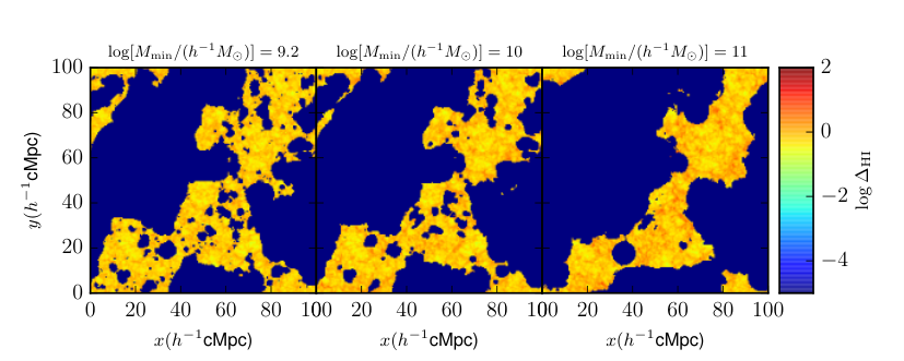
In order to understand how the multifractal nature of the HI density field is affected by , we compute for different values of the minimum mass. While doing this comparison, we fix the redshift to be and ensure that all the cases have the same value of the mass averaged neutral fraction, chosen to be . The maps of the HI density field for three values of and are shown in Figure 7. Clearly, there is some similarity in the overall structure of the HI field which follows from the fact that the haloes broadly trace the peaks of the underlying density field. We see that for smaller values of (left hand panel) there exist numerous ionized regions of smaller sizes that are not present for the higher . For the extreme value of , we see that the neutral regions are more concentrated and have larger sizes.
The behaviour of for different is shown in Figure 8. Clearly, the curves look quite similar in their shape, possibly because the broad structure of the HI density fields for the three cases are similar. We also find that there is hardly any difference in the results for and , thus indicating that is relatively insensitive to the value of . It might thus be possible to constrain the value of from the measurements of if lies in this range. However we also find that there is some significant difference in when takes a extremely high value of . The deviation of from the ambient value of 3 is more for higher values of . This is mainly because the HI density field is more clustered for higher as we have seen from the maps in Figure 7.
Finally, we investigate how the fractal dimensions behave when we modify the nature of the reionization process. By default, the excursion set based reionization models like the one used in this work are “inside-out” at large scales, in the sense that high density regions are ionized first followed by the low density voids (Furlanetto et al., 2004; Iliev et al., 2006; Mesinger & Furlanetto, 2007; Mesinger et al., 2011). This is because the ionizing sources are preferentially formed at large scale density peaks. Of course, this does not mean that the process is strictly inside-out at all scales, for example, a low density cell in the simulation box that is nearer to a source is more likely to be ionized earlier than a high density cell that is far away for any source. However, there is an additional complication which does not conform to this simple picture which arises from the “sinks” of ionizing photons (Miralda-Escudé et al., 2000). These are essentially the dense regions capable of self-shielding the radiation and thus remaining neutral. The presence of these sinks can make the reionization “outside-in” particularly at small scales (Choudhury et al., 2009). Accounting for these regions require either very high dynamic range simulations (Mesinger et al., 2015; Choudhury et al., 2015), or additional conditions for determining the ionized cells (Furlanetto & Oh, 2005; Choudhury et al., 2009; Sobacchi & Mesinger, 2014).
Rather than attempting to model the sinks (which can be quite expensive in terms of the computational requirements), we consider two extreme (and somewhat unrealistic) models, one where the reionization is strictly inside-out, while the other where it is strictly outside-in and study the resulting . These models are constructed by simply choosing a density threshold, and identifying all regions with density higher (lower) than this as ionized in the inside-out (outside-in) model (Jensen et al., 2013). We choose this threshold to obtain the desired . The maps for the two cases when are shown in Figure 9. It is obvious that the topology of reionization is completely different in the two cases. In the inside-out model (left), the neutral regions are somewhat diffuse as they trace the low density voids. The situation is exactly the opposite in the outside-in model (right) where the neutral regions are quite concentrated.
The fractal dimensions for these two models for a different are shown in Figure 10. The first point to note is that the values of are much closer to 3 for the inside-out model than the corresponding outside-in ones, thus implying that the HI distribution in the inside-out models are relatively more homogeneous at scales cMpc. The reason is that the dense and clustered cells are ionized first in the inside-out models, thus reducing the contrast in the HI field. On the other hand, the HI field in the outside-in models essentially trace the high density regions thus giving rise to less homogeneous structures. In fact, the shape of the curves approach that for the halo field as decreases. It is thus interesting that the fractal dimensions are quite sensitive to the nature of reionization, and thus could possibly distinguish between various scenarios. One should thus keep in mind that inclusion of photon sinks in the semi-numeric reionization models used in this paper can affect the behaviour of . Note that the values of for a reionization model with accurate treatment of the sinks are expected to be bound by the values obtained for these two extreme models, as long as the underlying cosmological density field remains the same.
5 Discussion and Conclusion
The first detection of the 21 cm signal from reionization, expected soon from the low-frequency experiments, is likely to be done by estimating the power spectrum, or equivalently the two-point correlation function, of the HI density field (Paciga et al., 2013; Dillon et al., 2014; Ali et al., 2015). However since the distribution of the ionized bubbles during the reionization epoch is expected to lead to a 21 cm signal that is highly non-Gaussian (Lidz et al., 2007; Wyithe & Morales, 2007), a significant amount of information would be contained in the higher order correlations of the distribution. In this work, we have explored the generalized correlation dimension (or the Minkowski-Bouligand dimension) as a diagnostic for understanding the nature of the HI distribution. The quantity has been used extensively for characterizing the multifractal nature of the galaxy distribution at low redshifts (Pietronero, 1987; Martinez & Jones, 1990; Coleman & Pietronero, 1992; Borgani, 1995; Sylos Labini et al., 1998; Bharadwaj et al., 1999; Martínez et al., 2001; Yadav et al., 2005; Sarkar et al., 2009; Yadav et al., 2010). The feature of is that it contains information about different higher order correlation functions and thus can probe the non-Gaussianity in the HI distribution (Borgani, 1995).
We use a semi-numeric simulation to generate the HI density field which is then used for estimating the at scales . Our main findings are as follows:
- •
The value of for the underlying baryonic density field is almost equal to (though not consistent with, within statistical error-bars) the ambient dimension 3 at our fiducial redshift , thus indicating that the density field can be taken to be homogeneous at scales . The for the corresponding halo field (or equivalently the distribution of galaxies weighed according to their ionizing emissivities), however, deviates significantly from 3 at these scales.
- •
The is almost equal to 3 for the HI density fluctuations field for mass averaged neutral fraction , thus indicating the distribution to be almost homogeneous when the IGM is significantly neutral. However, as the IGM gets more and more ionized, the becomes different from 3. For , the value of for is .
- •
The statistical errors on blow up for for , thus making these moments unsuitable for studying the HI field.
- •
The for the HI field is driven mainly by the distribution of the ionized regions, thus making them interesting quantities to study the growth and percolation of the ionized regions.
- •
The for is sensitive to the globally mass averaged , while its sensitivity to the minimum mass (in the range ) of ionizing haloes is relatively small. This indicates that the generalized correlation dimension can be used for constraining the global neutral fraction using upcoming observations.
- •
The form of the fractal dimension is, in principle, quite sensitive to the nature of reionization, e.g., whether the process is inside-out or outside-in. The presence of dense regions that are sinks of ionizing radiation, which are not included in the analysis here, can affect the value of .
The study presented in this work needs to be henceforth expanded in order to apply to the observed HI maps. In particular, one needs to calculate how the generalized dimension responds to the noise in the observations. Such calculations would help us infer the amount of observation time in different telescopes that would be required to distinguish between different ionization fractions. Also, it must be noted that the interferometric observations cannot measure the mean value of the field, thus one would have to work with a mean subtracted field . This would lead to mixing of the different moments in the data, however, the qualitative features presented in the work should still hold. We shall explore such related issues in a future work.
Acknowledgements
BB and TRS acknowledge the facilities at the IRC, DU. TRS acknowledges the R & D grant from Delhi University.
References
- Ali et al. (2015) Ali Z. S., et al., 2015, ApJ, 809, 61
- Bagla et al. (2008) Bagla J. S., Yadav J., Seshadri T. R., 2008, MNRAS, 390, 829
- Barkana & Loeb (2001) Barkana R., Loeb A., 2001, Phys. Rep., 349, 125
- Benson et al. (2003) Benson A. J., Bower R. G., Frenk C. S., Lacey C. G., Baugh C. M., Cole S., 2003, ApJ, 599, 38
- Bharadwaj & Pandey (2005) Bharadwaj S., Pandey S. K., 2005, MNRAS, 358, 968
- Bharadwaj et al. (1999) Bharadwaj S., Gupta A. K., Seshadri T. R., 1999, A&A, 351, 405
- Borgani (1995) Borgani S., 1995, Phys. Rep., 251, 1
- Borgani et al. (1993) Borgani S., Murante G., Provenzale A., Valdarnini R., 1993, Phys. Rev. E, 47, 3879
- Bowman et al. (2011) Bowman J. D., Morales M. F., Hewitt J. N., MWA Collaboration 2011, in American Astronomical Society Meeting Abstracts #218. p. 132.06
- Choudhury & Ferrara (2006) Choudhury T. R., Ferrara A., 2006, ArXiv Astrophysics e-prints,
- Choudhury et al. (2009) Choudhury T. R., Haehnelt M. G., Regan J., 2009, MNRAS, 394, 960
- Choudhury et al. (2015) Choudhury T. R., Puchwein E., Haehnelt M. G., Bolton J. S., 2015, MNRAS, 452, 261
- Coleman & Pietronero (1992) Coleman P. H., Pietronero L., 1992, Physica A Statistical Mechanics and its Applications, 185, 45
- Cooray (2005) Cooray A., 2005, MNRAS, 363, 1049
- Dillon et al. (2014) Dillon J. S., et al., 2014, Phys. Rev. D, 89, 023002
- Feder (1988) Feder J., 1988, Fractals. New York: Springer US
- Furlanetto & Oh (2005) Furlanetto S. R., Oh S. P., 2005, MNRAS, 363, 1031
- Furlanetto et al. (2004) Furlanetto S. R., Zaldarriaga M., Hernquist L., 2004, ApJ, 613, 1
- Furlanetto et al. (2006) Furlanetto S. R., Oh S. P., Briggs F. H., 2006, Phys. Rep., 433, 181
- Geil & Wyithe (2008) Geil P. M., Wyithe J. S. B., 2008, MNRAS, 386, 1683
- Ghara et al. (2015) Ghara R., Choudhury T. R., Datta K. K., 2015, MNRAS, 447, 1806
- Gleser et al. (2006) Gleser L., Nusser A., Ciardi B., Desjacques V., 2006, MNRAS, 370, 1329
- Gnedin (2016) Gnedin N. Y., 2016, ApJ, 825, L17
- Gnedin & Hui (1998) Gnedin N. Y., Hui L., 1998, MNRAS, 296, 44
- Gnedin et al. (2008) Gnedin N. Y., Kravtsov A. V., Chen H.-W., 2008, ApJ, 672, 765
- Greig et al. (2016) Greig B., Mesinger A., Pober J. C., 2016, MNRAS, 455, 4295
- Hong et al. (2014) Hong S. E., Ahn K., Park C., Kim J., Iliev I. T., Mellema G., 2014, Journal of Korean Astronomical Society, 47, 49
- Iliev et al. (2006) Iliev I. T., Mellema G., Pen U.-L., Merz H., Shapiro P. R., Alvarez M. A., 2006, MNRAS, 369, 1625
- Jensen et al. (2013) Jensen H., et al., 2013, MNRAS, 435, 460
- Kimm & Cen (2014) Kimm T., Cen R., 2014, ApJ, 788, 121
- Kulkarni et al. (2016) Kulkarni G., Choudhury T. R., Puchwein E., Haehnelt M. G., 2016, MNRAS, 463, 2583
- Lee et al. (2008) Lee K.-G., Cen R., Gott III J. R., Trac H., 2008, ApJ, 675, 8
- Lidz et al. (2007) Lidz A., Zahn O., McQuinn M., Zaldarriaga M., Dutta S., Hernquist L., 2007, ApJ, 659, 865
- Mandelbrot (1982) Mandelbrot B. B., 1982, The Fractal Geometry of Nature. San Francisco: Freeman & Co.
- Martinez & Jones (1990) Martinez V. J., Jones B. J. T., 1990, MNRAS, 242, 517
- Martínez & Saar (2002) Martínez V. J., Saar E., 2002, Statistics of the Galaxy Distribution. Chapman & Hall
- Martínez et al. (2001) Martínez V. J., López-Martí B., Pons-Bordería M.-J., 2001, ApJ, 554, L5
- Mellema et al. (2006) Mellema G., Iliev I. T., Pen U.-L., Shapiro P. R., 2006, MNRAS, 372, 679
- Mesinger & Furlanetto (2007) Mesinger A., Furlanetto S., 2007, ApJ, 669, 663
- Mesinger et al. (2011) Mesinger A., Furlanetto S., Cen R., 2011, MNRAS, 411, 955
- Mesinger et al. (2015) Mesinger A., Aykutalp A., Vanzella E., Pentericci L., Ferrara A., Dijkstra M., 2015, MNRAS, 446, 566
- Miralda-Escudé et al. (2000) Miralda-Escudé J., Haehnelt M., Rees M. J., 2000, ApJ, 530, 1
- Mitra et al. (2015) Mitra S., Choudhury T. R., Ferrara A., 2015, MNRAS, 454, L76
- Mittal & Seshadri (2002a) Mittal A. K., Seshadri T. R., 2002a, Resonance, 7, 6
- Mittal & Seshadri (2002b) Mittal A. K., Seshadri T. R., 2002b, Resonance, 7, 39
- Paciga et al. (2011) Paciga G., et al., 2011, MNRAS, 413, 1174
- Paciga et al. (2013) Paciga G., et al., 2013, MNRAS, 433, 639
- Parsons et al. (2014) Parsons A. R., et al., 2014, ApJ, 788, 106
- Pietronero (1987) Pietronero L., 1987, Physica A Statistical Mechanics and its Applications, 144, 257
- Pillepich et al. (2007) Pillepich A., Porciani C., Matarrese S., 2007, ApJ, 662, 1
- Planck Collaboration et al. (2014) Planck Collaboration et al., 2014, A&A, 571, A16
- Planck Collaboration et al. (2016a) Planck Collaboration et al., 2016a, preprint, (arXiv:1605.03507)
- Planck Collaboration et al. (2016b) Planck Collaboration et al., 2016b, A&A, 594, A13
- Pritchard & Loeb (2012) Pritchard J. R., Loeb A., 2012, Reports on Progress in Physics, 75, 086901
- Puchwein & Springel (2013) Puchwein E., Springel V., 2013, MNRAS, 428, 2966
- Razoumov & Sommer-Larsen (2010) Razoumov A. O., Sommer-Larsen J., 2010, ApJ, 710, 1239
- Saiyad Ali et al. (2006) Saiyad Ali S., Bharadwaj S., Pandey S. K., 2006, MNRAS, 366, 213
- Sarkar et al. (2009) Sarkar P., Yadav J., Pandey B., Bharadwaj S., 2009, MNRAS, 399, L128
- Schneider et al. (2008) Schneider R., Salvaterra R., Choudhury T. R., Ferrara A., Burigana C., Popa L. A., 2008, MNRAS, 384, 1525
- Shimabukuro et al. (2015) Shimabukuro H., Yoshiura S., Takahashi K., Yokoyama S., Ichiki K., 2015, MNRAS, 451, 467
- Shimabukuro et al. (2016) Shimabukuro H., Yoshiura S., Takahashi K., Yokoyama S., Ichiki K., 2016, MNRAS, 458, 3003
- Sobacchi & Mesinger (2014) Sobacchi E., Mesinger A., 2014, MNRAS, 440, 1662
- Springel (2005) Springel V., 2005, MNRAS, 364, 1105
- Sylos Labini et al. (1998) Sylos Labini F., Montuori M., Pietronero L., 1998, Phys. Rep., 293, 61
- Watkinson & Pritchard (2015) Watkinson C. A., Pritchard J. R., 2015, MNRAS, 454, 1416
- Wise et al. (2014) Wise J. H., Demchenko V. G., Halicek M. T., Norman M. L., Turk M. J., Abel T., Smith B. D., 2014, MNRAS, 442, 2560
- Wyithe & Loeb (2013) Wyithe J. S. B., Loeb A., 2013, MNRAS, 428, 2741
- Wyithe & Morales (2007) Wyithe J. S. B., Morales M. F., 2007, MNRAS, 379, 1647
- Yadav et al. (2005) Yadav J., Bharadwaj S., Pandey B., Seshadri T. R., 2005, MNRAS, 364, 601
- Yadav et al. (2010) Yadav J. K., Bagla J. S., Khandai N., 2010, MNRAS, 405, 2009
- Yoshiura et al. (2015) Yoshiura S., Shimabukuro H., Takahashi K., Momose R., Nakanishi H., Imai H., 2015, MNRAS, 451, 266
- Yoshiura et al. (2016) Yoshiura S., Shimabukuro H., Takahashi K., Matsubara T., 2016, preprint, (arXiv:1602.02351)
- Zahn et al. (2007) Zahn O., Lidz A., McQuinn M., Dutta S., Hernquist L., Zaldarriaga M., Furlanetto S. R., 2007, ApJ, 654, 12
- van Haarlem et al. (2013) van Haarlem M. P., et al., 2013, A&A, 556, A2