Resonant Floquet scattering
of ultracold atoms
Abstract
In systems of ultracold atoms, pairwise interactions are resonantly enhanced by the application of an oscillating magnetic field that is parallel to the spin-quantization axis of the atoms. The resonance occurs when the frequency of the applied field is precisely tuned near the transition frequency between the scattering atoms and a diatomic molecule. The resulting cross section can be made more than two orders of magnitude larger than the cross section in the absence of the oscillating field. The low momentum resonance properties have a universal description that is independent of the atomic species. To arrive at these conclusions, we first develop a formal extension of Floquet theory to describe scattering of atoms with time-periodic, short-range interaction potentials. We then calculate the atomic scattering properties by modeling the atomic interactions with a square well potential with oscillating depth and then explicitly solving the time-dependent Schrödinger equation. We then apply the Floquet formalism to the case of atoms scattering with a contact interaction described by a time-periodic scattering length, obtaining analytic results that agree with those obtained by solving the time-dependent Schrödinger equation.
Eric Braaten \degreeDoctor of Philosophy \memberLouis DiMauro \memberIlya Gruzberg \memberUlrich Heinz \authordegreesB.S, B.A. \graduationyear2016 \unitGraduate Program in Physics
To my wife and children.
Acknowledgements.
I express my deep gratitude to Eric Braaten, my research advisor and mentor. Over the past five years, he has pursued my development as a physicist by tirelessly answering my questions, by continuously offering well-reasoned feedback and advice, and by generously providing me with many opportunities to attend scientific conferences and workshops. I owe much of what I am as a physicist to Eric. I owe more than I can express to my wife. Her love and support keep me afloat. I thank my mom, dad, and brothers for their continued prayers and encouragement. I also thank Rich Schelp for his friendship, mentorship, and for helping me take my first steps as a physicist. I also thank the local community of graduate students and postdocs. In particular, I thank Christian Langmack, Chuck Bryant, Sushant More, Abhishek Mohapatra, Hong Zhang, Xiangyu Yin, and Shaun Hampton for their friendship and for making the OSU physics department a fun and intellectually stimulating environment. Without them and many others, life as a graduate student would have been very dull indeed. I must also thank the physics administrative staff. I am particularly grateful to Kris Dunlap whose patience with me appears to be never-ending.September 2007–May 2011BS in Physics and BA in Mathematics, Erskine College, Due West, South Carolina
\dateitemSeptember 2011–August 2016PhD in Physics, Ohio State University, Columbus, Ohio
{publist}
Avalanche mechanism for atom loss near an atom-dimer Efimov resonance
Christian Langmack, D. Hudson Smith, and Eric Braaten
Phys. Rev. A 86, 022718 (2012) [arXiv:1205.2683]
Avalanche mechanism for the enhanced loss of ultracold atoms
Christian Langmack, D. Hudson Smith, and Eric Braaten
Phys. Rev. A 87, 023620 (2013) [arXiv:1209.4912]
Atom loss resonances in a Bose-Einstein condensate
Christian Langmack, D. Hudson Smith, and Eric Braaten
Phys. Rev. Lett. 111, 023003 (2013) [arXiv:1302.5925]
Two-body and three-body contacts for identical bosons near unitarity
D. Hudson Smith, Eric Braaten, Daekyoung Kang, and Lucas Platter
Phys. Rev. Lett. 112, 110402 (2014) [arXiv:1309.6922]
Selection rules for hadronic transitions of XYZ mesons
Eric Braaten, Christian Langmack, and D. Hudson Smith
Phys. Rev. Lett. 112, 222001 (2014) [arXiv:1401.7351]
Born-Oppenheimer approximation for the XYZ mesons
Eric Braaten, Christian Langmack, and D. Hudson Smith
Phys. Rev. D 90, 014044 (2014) [arXiv:1402.0438]
Association of atoms into universal dimers using an oscillating magnetic field
Christian Langmack, D. Hudson Smith, and Eric Braaten
Phys. Rev. Lett. 114, 103002 (2015) [arXiv:1406.7313]
Inducing resonant interactions in ultracold atoms with a modulated magnetic field
D. Hudson Smith
Phys. Rev. Lett. 115, 193002 (2015) [arXiv:1503.02688]
Induced two-body scattering resonances from a square-well potential
with oscillating depth
D. Hudson Smith
EPJ Web of Conf. 113, 02005 (2015)
Dynamics of small trapped one-dimensional Fermi gas
under oscillating magnetic field
X. Y. Yin, Yangqian Yan, and D. Hudson Smith
Phys. Rev. A 94, 043639 (2016) [arXiv:1608.06966]
Physics {studieslist} \studyitemAtomic physics: Universal aspects of ultracold atomic gases
Chapter 1 Introduction
One of the great achievements of modern physics is the quantum mechanical description of matter. On a microscopic level, matter behaves in exciting and counterintuitive ways. Particles behave not like points in space but instead like waves that extend over a region of space. Particle energies can take on discrete values. Particles come in two basic types called bosons and fermions, which have dramatically different quantum behavior. The quantum description of matter has led to accurate, systematic explanations for diverse phenomena, ranging from the chemical properties of elements in the periodic table to superconductivity in metals at very low temperatures. More recently, novel experiments with ultracold trapped atoms have begun to unveil the intricacies of the microscopic, quantum-mechanical world in unprecedented ways. These experiments study trapped gases of atoms that have been cooled to such low temperatures that a particle’s quantum mechanical nature takes over.
A unique feature of cold atomic gases is the ability to experimentally adjust the strength of interactions between particles. This tunability makes it possible to measure the properties of cold atomic gases all the way from the non-interacting regime, where the particles have no influence on one another, to the regime with infinitely strong interactions. This control over the quantum nature of atoms has led to unprecedented breakthroughs in few- and many-body physics.
For ultracold atoms, a convenient measure of particle interactions is the -wave scattering length . Roughly speaking, the magnitude of corresponds to the distance over which particles feel each other, and the sign of indicates whether the interaction is attractive or repulsive. At very low energy the 2-body elastic cross section for distinguishable particles is simply
| (1.1) |
For large , the cross section becomes large, signaling strong atomic interactions. The experimental techniques for controlling the strength of atomic interactions involve the manipulation of the effective scattering length . By the careful application of external magnetic or optical fields, the scattering length can be made resonantly large, positive or negative.
In this thesis, we discuss a new technique for resonantly enhancing the effective interaction between atoms, which we term Modulated Magnetic Feshbach Resonance (MMFR). This technique, involves the application of an oscillating magnetic field near a precise frequency. Microscopically, the effect of this field is to modulate the strength of the 2-atom interaction potential in time. This modulated potential can significantly alter the scattering properties of the 2-body system. The oscillating potential can inject or remove energy from the scattering particles while they are in the scattering region. The potential injects or removes energy in quanta of , where is the oscillation frequency. This is more complicated than scattering from a time-independent potential, for which energy is conserved, but it is less complicated than scattering from a potential with arbitrary time dependence for which energy conservation can be violated by arbitrary amounts. Figure 1.1 gives a heuristic picture of how the oscillating potential splits an incoming wave into multiple, evenly-spaced energy components.
This basic property of scattering from time-periodic potentials leads to the possibility of experimentally tuning the effective interactions between particles by tuning the oscillation frequency . In fact, as we will show, for potentials supporting bound states (as in Fig. 1.1), a scattering resonances is induced if is tuned near the transition frequency between the scattering state of the scattering particles and the bound state. Of course, as a prerequisite, the experimentalist must be able to modulate the effective interaction potential between particles. We will show in Chapter that the effective interactions between cold, neutral atoms can be modulated by the application of an oscillating magnetic field. We find that the effective cross section can be enhanced by several orders of magnitude.
This thesis is organized as follows: In Chapter 2, we discuss the basic properties of ultracold atomic gases, providing the physical context for our later discussions. In Chapter 3, as a prerequisite for understanding scattering of atoms in the presence of an oscillating magnetic field, we review scattering in the absence of such a field. In Chapter 4, we discuss Floquet theory, which provides a natural framework for dealing with time-periodic potentials. Chapter begins the unique contributions of this thesis. There we derive an extension of Floquet theory to describe 2-body scattering with a short-range, time-periodic interaction potential. In Chapter , we derive the scattering properties of atoms with a short-range time-periodic potential modeled by a square-well with oscillating depth. In Chapter , we use the Floquet scattering formalism derived in Chapter to calculate the scattering properties of atoms with an explicitly zero-range time-periodic potential. We conclude in Chapter .
Chapter 2 Ultracold atomic gases
Modern experiments with ultracold gases have demonstrated the unprecedented ability to create and manipulate macroscopic samples of atoms whose properties are governed by the underlying quantum statistics of the particles. The creation of such quantum gases relies upon advanced technologies for trapping and cooling the atoms. Once created, the manipulation of ultracold gases can be achieved at the quantum level by tuning the effective interactions between the particles. This ability has led to many advances in our understanding of the role of interactions in quantum matter and has potentially many applications in the field of quantum engineering. This chapter discusses the basic properties of ultracold atomic gases, providing the physical context for our later discussions. Refs. [UBG_review, UFG_review] provide extensive reviews of the properties of cold Bose and Fermi gases as well as the associated experimental techniques.
In Section 2.1, we review the properties of alkali atoms, which are the most common species used in experiments with ultracold atomic gases. In Section 2.2, we discuss the theoretical motivations and experimental procedures for cooling atoms. In Section 2.3, we discuss techniques for tuning the effective interactions between atoms.
2.1 Alkali atoms
The types of neutral atoms that are most easily cooled to ultralow temperatures and whose interactions can be most easily manipulated are the alkali atoms more massive than hydrogen (H) and less massive than francium (Fr). They are lithium (Li), sodium (Na), potassium (K), rubidium (Rb), and cesium (Cs). Hydrogen is difficult to cool due to its small mass, and francium is rarely used due to its relatively short half-life of minutes [feshbach, francium]. The ability to cool and manipulate the alkali atoms largely arises from their simple electronic structure, which leads to a relatively simple response of these atoms to a magnetic field, as discussed in Section 2.1.1. At low energies, the interaction properties of the alkali atoms are governed by their van der Waals interaction potentials, as discussed in Section 2.1.2.
2.1.1 Hyperfine spin states
An alkali atom in its electronic ground state has multiple spin states. There are two contributions to its spin: the electronic spin with quantum number and the nuclear spin with quantum number . The spin states can be labeled , where and specify the eigenvalues of and . The Hamiltonian for a single atom includes a hyperfine term that can be expressed in the form
| (2.1) |
This term splits the ground state of the atom into two hyperfine multiplets with energies differing by . The sum of the electronic and nuclear spin is called the hyperfine spin . The eigenstates of are labeled by the quantum numbers and which specify the eigenvalues of and . The eigenvalues of are
| (2.2) |
The two hyperfine multiplets of an alkali atom consist of states with and states with . For example, a 7Li atom has nuclear spin quantum number . The two hyperfine multiplets consist of five states with and three states with . The multiplet is higher in energy by . The frequency associated with the hyperfine splitting is MHz [ScatteringModelsBraaten, feshbach].
In the presence of a magnetic field , the Hamiltonian for a single atom has a magnetic term. The magnetic moment of the atom is dominated by the term proportional to the spin of the electron: = . The magnetic moment of an alkali atom such as Li is approximately that of the single electron in the outermost shell: , where is the Bohr magneton. The magnetic term in the Hamiltonian can be expressed in the form
| (2.3) |
If , this term splits the two hyperfine multiplets of an alkali atom into hyperfine states. In a weak magnetic field satisfying , each hyperfine multiplet is split into equally-spaced Zeeman levels . In a strong magnetic field satisfying , the states are split into a set of states with whose energies increase linearly with and a set of states with whose energies decrease linearly with . Each of those states is the continuation in of a specific hyperfine state at small . It is convenient to label the states by the hyperfine quantum numbers and for general , in spite of the fact that those states are not eigenstates of if . We denote the eigenstates of by and their eigenvalues by . The two eigenstates with the maximal value of are independent of :
| (2.4) |
Their eigenvalues are exactly linear in :
| (2.5) |
If , each of the other eigenstates is a linear superposition of the two states and .
The dependence of the hyperfine energy levels of 7Li atoms on the magnetic field is illustrated in Fig. 2.1. At , the hyperfine multiplets with and are split by . The magnetic energy scale is comparable to the hyperfine splitting when is about 287 Gauss. At higher magnetic fields, the four states decrease linearly with , while the four states increase linearly.
2.1.2 Interaction potentials
Due to the large separation of mass scales between the atomic nucleus and the electrons, the atomic interactions are very accurately characterized by the Born-Oppenheimer (BO) potentials for the atoms. Each potential can be labeled by the combination of quantum numbers , where is the total electronic spin quantum number, (or 1, 2, 3, ) specifies the total orbital angular momentum of the atom pair, and (or gerade/ungerade) specifies the electronic inversion symmetry (only present for identical atoms). An electronic configuration is gerade (ungerade) if the phase of the wavefunction is even (odd) with respect to inversion through the molecular center of mass. The BO potential for an atom pair in the configuration equals the potential energy of the atom pair in that configuration as a function of the separation of the atomic nuclei [feshbach].
We consider alkali atoms in their ground state for which . In that case all of the Born-Oppenheimer potentials are isotropic: they only depend on the nuclear separation . Two separated alkali atoms in their ground state individually have zero orbital angular momentum and electron spin of 1/2. The total electronic spin can therefore be , in which case the system is gerade, or , in which case the system is ungerade. Thus, the relevant BO potentials for scattering alkali atoms are and . These BO potentials for the 6Li system are plotted in Fig. 2.2.
For -state atoms, the leading term in the BO potential at large are independent of the hyperfine spin configuration. The large- potentials can then be expressed in terms of a single parameter, , which depends on the choice of atomic species, but not on the hyperfine spins of the atoms:
| (2.6) |
is the van der Waals potential. The natural length scale for this potential is
| (2.7) |
where is the reduced mass of the atom pair. The corresponding energy scale is
| (2.8) |
Table 2.1 gives and for several alkali atoms. In units of Boltzmann’s constant , the typical van der Waals energy scale is mK, which is three orders of magnitude larger than the typical collision energy in an ultracold gas experiment K. As a result, the atomic scattering properties are only sensitive to the low-energy (long-distance) details of the interatomic potential. Moreover, if the BO potential supports a bound state with binding energy much smaller than , the properties of such a bound state are only sensitive to the long range van der Waals potential [ScatteringModelsBraaten, feshbach, Gao1998, Gao2000].
| species | mass | Ref. | |||
|---|---|---|---|---|---|
| (amu) | () | (mK) | (MHz) | ||
| 6Li | 6.0151223 | 31.26 | 29.47 | 614.1 | [Yan1996] |
| 23Na | 22.9897680 | 44.93 | 3.732 | 77.77 | [Derevianko1999] |
| 40K | 39.9639987 | 64.90 | 1.029 | 21.44 | [Derevianko1999] |
| 40Ca | 39.962591 | 56.39 | 1.363 | 28.40 | [Porsev2002] |
| 87Rb | 86.909187 | 82.58 | 0.2922 | 6.089 | [vanKempen2002] |
| 133Cs | 132.905429 | 101.0 | 0.1279 | 2.666 | [Chin2004] |
2.2 Dilute, cold gases
In this section we discuss the importance of the density and temperature of atomic gases. We also describe some of the techniques used to create dilute, cold gases.
2.2.1 The low-density regime
Consider an atomic gas with particle number density . The diluteness of the gas is measured by the dimensionless parameter where is the range of the 2-body interaction potential between the two different spin states. When , the spacing between particles is larger than the range of the potential, and, under ordinary circumstances, the particles interact very weakly. Such a gas is approximately “ideal” and the effects of interactions can be incorporated perturbatively. When , the spacing between particles is comparable to or less than the range of the potential, and the effects of interactions cannot generally be incorporated perturbatively. If the system has a resonant -wave scattering length such that , then replaces as the relevant length scale for measuring diluteness. In that case, dilute gases satisfy [pethicbec, Braaten:2001ay].
2.2.2 The low-temperature regime
A particle with momentum has de Broglie wavelength . describes the spacial extent of the wave function of a particle with momentum . The typical de Broglie wavelength for a particle with mass in a gas at temperature is of the order of the thermal de Broglie wavelength,
| (2.9) |
can be regarded as the uncertainty in the position of a typical particle in a gas at temperature . At high temperatures, is small, and the constituents of the gas behave like classical, point-like particles. At low temperatures, particles have larger spacial extent. When this extent becomes on the same order as the inter-particle spacing (, where is the particle density), the quantum mechanical nature of the particles modifies the properties of the system. For , the particle behavior is completely governed by either Bose-Einstein statistics in the case of bosons or Fermi-Dirac statistics in the case of fermions. Thus, the pursuit of low temperatures is partly motivated by a desire to isolate and study the unique bosonic or fermionic statistical properties of matter.
Also, as discussed in Sec. 2.1.2, the typical collision energy is of the same order as the temperature of the gas multiplied by . If that energy scale is much less than the van der Waals energy scale , the physical properties of the gas are only sensitive to the long-distance details of the scattering potential. This leads to a dramatic simplification in the theoretical description of ultracold gases, requiring only the van der Waals coefficient to describe the low-energy physics.
2.2.3 Trapping and cooling ultracold gases
We will discuss a standard approach to creating and trapping an ultracold atomic gas. There are numerous variants on the general pattern discussed here. For a more thorough review, see Refs. [UBG_review, UFG_review]. Cooling occurs in several stages, over which the temperature of the gas can be reduced by about orders of magnitude. An initial beam of highly energetic atoms () passes through a Zeeman slower, which uses doppler cooling to reduce the energy to . The atoms are then transferred to a magneto-optical trap (MOT), where a combination of typically six intersecting lasers combined with a non-uniform magnetic field confine and cool the cloud. The MOT doppler-cools the cloud to . The atoms are then transferred into an optical trap, which uses a single, tightly-focused beam to confine the atoms by the interaction between the electric field-gradient and the electric dipole moment of the atom. The depth of the optical trap can then be incrementally lowered. This allows the high-momentum component of the trapped atoms to escape, lowering the average temperature of the remaining atoms. This technique, called evaporative cooling, cools the atoms to .
2.3 Tuning interactions
Multiple techniques exist for manipulating the effective interactions between neutral alkali-metal atoms. These techniques all exploit a coupling between the scattering state of interest and a two-atom bound state, often called the resonance state. The differences between these techniques lie in the choice of resonance state and in how the coupling between the scattering and resonance state is achieved. Here we briefly review the established techniques for controlling the effective interactions.
Magnetic Feshbach resonance.
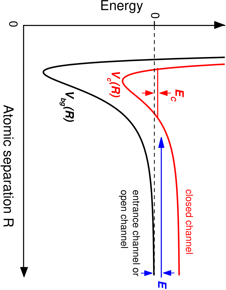
Magnetic Feshbach resonance (MFR) [feshbach] is the most powerful and versatile method to date for manipulating the effective interactions between atoms. In MFR a constant magnetic field applied along the spin quantization axis of the atoms is used to couple the scattering state to a molecular state in a second hyperfine spin channel. Figure 2.3 illustrates the interaction potentials for the scattering channel and the channel containing the bound state. The energy difference between the scattering threshold and the bound state is modified by the application of a magnetic field , because the magnetic moment of the bound state differs from the magnetic moment of the scattering state. A scattering resonance occurs at the magnetic field value where the energy of the bound level equals the scattering threshold energy. The corresponding -dependent -wave scattering length is shown in Fig. 2.4. Near , is a simple function of :
| (2.10) |
where is the background scattering length, is the distance from the resonance to the nearest zero crossing, and is non-zero only if the colliding atoms have a spin-relaxation scattering channel.
While extremely useful in many scenarios, MFR is limited to atomic systems where scattering atoms can be brought to degeneracy with a bound state in a coupled channel by the application of a magnetic field of a reasonable magnitude. The properties of the associated resonance are then completely determined by the microscopic details of the interatomic potential and may not be favorable for experimental use.

Optical Feshbach Resonance
In optical Feshbach resonance (OFR) [Shlyapnikov, Julienne_1999, Lett_2000, Grimm_2004, Grimm_2005], laser light that is slightly detuned from a transition between the scattering atoms and an electronically excited -wave molecule induces a resonance in the scattering length. Figure 2.5 presents an experimental realization of OFR in 87Rb. One advantage of OFR over MFR is that laser light can be switched much more rapidly than electrostatic magnetic fields. In addition, the properties of an OFR depend upon the intensity of the laser, giving some control over the strength and width of the resonance. OFR has major limitations for alkali-metal atoms because the rapid spontaneous decay of the resonance molecule results in dramatic atom losses and severely limits the maximum value of the scattering length. This is demonstrated experimentally in panel (a) of Fig. 2.5.

Radio-frequency and Microwave Feshbach Resonance
In radio-frequency
Feshbach resonance (rfFR) and microwave Feshbach resonance (mwFR) [Julienne_rfFR_2009, Schmiedmayer_rfFR_2010, Dalibard_mwFR_2010], an oscillating magnetic field that is perpendicular to the spin-quantization axis of the atoms couples an atom pair to a molecule in another hyperfine channel, thereby modifying or inducing a resonance in the scattering length. These methods allow some control over the scattering length without introducing dramatic atom loss. One disadvantage of rf/mwFR is that the coupling between an atom pair and the resonance molecule tends to be very small, leading to very small enhancement of the real part of the scattering length. Also, it is difficult to produce large-amplitude rf and mw fields. Figure 2.6 shows a theoretical prediction for a rfFR in 87Rb.
Modulated Magnetic Feshbach Resonance
We now discuss a new mechanism, modulated-magnetic Feshbach resonance (MMFR), for resonantly enhancing the scattering length in ultracold gases. MMFR was first introduced in Ref. [Hudson_2015]. This mechanism is related to modulated-magnetic spectroscopy or wiggle spectroscopy, which has been used to measure molecular binding energies and other properties for several alkali-metal atoms [Wieman2005, PhysRevLett.95.190404, Inguscio0808, Chin_2009, Khaykovich1201, Hulet1302]. In wiggle spectroscopy and MMFR, an oscillating magnetic field
| (2.11) |
is applied parallel to the spin-quantization axis of the atoms and near the transition frequency between an atom pair and a shallow bound state in the scattering channel. The resulting time-dependent scattering length is given by Eq. (2.10) with replaced by . For sufficiently small values of , the resulting scattering length is linear in :
| (2.12) |
where
| (2.13) |
The time-dependent scattering length in Eq. (2.12) has a profound effect on the scattering properties of the atoms. Experiments in wiggle spectroscopy have demonstrated that the oscillating field induces transitions to the molecular state which, if unstable, will then decay, leading to measurable atom loss. What had not been realized prior to Ref. [Hudson_2015] was that under the circumstances of wiggle spectroscopy experiments, the oscillating field resonantly enhances the elastic scattering properties of the atoms, giving rise to the effective frequency-dependent scattering length
| (2.14) |
This equation is a close parallel to Eq. (2.10). For near a MFR, the resonance parameters , , and in Eq. (2.14) are universal in a sense that will be made precise in . Figure 2.7 shows predictions for the scattering length in the vicinity of a MMFR.
In Eq. (2.14) the imaginary part of arises from collisions in which a pair of low-energy atoms emits one or more quanta of frequency and forms a molecule. A complex also arises when controlling the scattering length of 85Rb with MFR because the only accessible broad resonance occurs in a hyperfine configuration with a spin-relaxation channel. However, this has not prevented pioneering studies of few- and many-body physics using 85Rb atoms [Wieman2002, Wieman2005, Robins2011, Jin2012, Cornish2013, Jin2014].
The frequencies needed for MMFR are much lower than for rf/mwFR. This allows for larger amplitudes of the oscillating magnetic field. Also, because of the parallel polarization of the oscillating field, the coupling between an atom pair and the bound state can be much stronger than for rf/mwFR. Larger oscillation amplitudes combined with stronger coupling results in greater enhancement of the scattering length. In Chapters and , we calculate the scattering properties of atoms in the presence of a MMFR.
Chapter 3 Scattering theory
Before examining the scattering of neutral atoms in the presence of an oscillating magnetic field, we must first understand scattering in the absence of such a field. Here we aim to present the essential details. For complete discussions see Refs. [taylor_scattering_thy, newton_scattering_thy]. We first review the basic concepts of scattering theory in Sec. 3.1 and apply those concepts to the low-energy scattering of alkali-metal atoms. In Section 3.2 we examine the scattering properties of atoms that have an -wave scattering length that is much larger than all other intrinsic length scales. We conclude in Sec. 3.3 by showing that systems with -wave universality are succinctly described by an effective quantum field theory. This field-theoretic description will be particularly useful when discussing time-periodic, zero-range interactions in Chapter .
3.1 Basic scattering theory
In this section, we briefly review the scattering of two distinguishable particles with short-range interaction potentials. Let , , and be the kinetic energy operator, the short-range interaction potential, and the wavevector for the 2-body system, respectively. To describe the fate of two incident particles, we should solve the time-dependent Schrödinger equation (TDSE):
| (3.1) |
The solution for must satisfy the asymptotic boundary condition:
| (3.2) |
where is the relative momentum and is the mass. is an eigenstate of :
| (3.3) |
By using the boundary condition in Eq. (3.2), we are tacitly assuming that the desired solution does not depend upon the width of the incident physical wave packet. As discussed in many scattering theory texts, this is always the case for stationary potentials (see e.g. Ref. [taylor_scattering_thy]).
In the following sections, we will discuss the machinery for solving and understanding the TDSE, Eq. (3.1), subject to the asymptotic boundary condition, Eq. (3.2). Our goal is not to re-derive the basic results of scattering theory in full, but rather to provide a basis for comparison once we move to the problem of scattering from time-periodic potentials. Many of the results in the latter case are highly analogous to the results that we will now discuss.
3.1.1 Lippmann-Schwinger equation
We begin our discussion of scattering theory by deriving the Lippmann-Schwinger equation (LSE). The LSE fully encodes the physics of the TDSE, Eq. (3.1), and the asymptotic boundary condition, Eq. (3.2), into one equation. This equation will prove very useful in the development of the scattering formalism and as a starting point for actual calculations.
Due to conservation of energy, we expect the time-dependent Schrödinger equation in Eq. (3.1) to have solutions of the form
| (3.4) |
where is time independent. Inserting this into the TDSE and dropping the overall time-dependent phase gives
| (3.5) |
We can immediately write down a formal solution to Eq. (3.5) that also satisfies the boundary condition in Eq. (3.2):
| (3.6) |
is the noninteracting Green’s function:
| (3.7) |
where the prescription ensures that we include only causal solutions (i.e. the propagation of particles forward in time). By acting the operator on both sides of Eq. (3.6), we recover Eq. (3.5).
Equation (3.6) is the Lippmann-Schwinger equation (LSE). The LSE fully encodes the information from both the time-dependent Schödinger equation and the boundary condition in the asymptotic past. It is not a solution in the practical sense because the wavevector depends upon itself operated upon by . Nevertheless, the LSE naturally leads to methods for calculating the desired physical quantities.
3.1.2 Asymptotic wavefunction
We can extract scattering observables from knowledge about the wavefunction in the region where the distance between the particles is much larger than the range of the potential. Using the LSE, we can extract the wavefunction in the region of large separation.
Projecting the Lippmann-Schwinger equation into position space gives
| (3.8) |
is the free position-space Green’s function:
| (3.9) |
where is defined in Eq. (3.7). In the region where the particle separation is much greater than the range of the potential, Eq. (3.8) takes the form
| (3.10) |
To obtain Eq. (3.10) we have dropped all terms that fall faster than . This equation manifestly satisfies the asymptotic boundary condition in Eq. (3.2), since the only incoming plane wave component equals the one specified by the boundary condition. All other components are spherical outgoing waves.
Defining the scattering amplitude
| (3.11) |
we arrive at the standard form of the asymptotic wavefunction :
| (3.12) |
In Eq. (3.11), the dependence on the incident relative momentum is hidden in . is the scattering amplitude for incident scatterers with relative momentum and center of mass energy to exit with momentum and energy . Note that the asymptotic wavefunctions only depend on amplitudes that satisfy the on-shell condition .
3.1.3 Scattering cross section
The quantum mechanical scattering from a short-range potential is fully characterized by the scattering amplitude defined in Eq. (3.11). In particular, we are interested in the differential cross section for the incoming scatterers with momentum to exit into the solid angle . The differential cross section is:
| (3.13) |
where is the differential rate of probability flow, and is the magnitude of the incident particle current density. equals the scattered current density into the solid angle , , dotted with the corresponding area element. Dividing out an overall factor of this gives
| (3.14) |
The scattered current density is determined by the scattered part of the asymptotic wavefunction defined in Eq. (3.12):
| (3.15) |
The scattered current density at large separations is
| (3.16) |
Inserting this result into Eq. (3.14), we find
| (3.17) |
The magnitude of the incident current density is simply
| (3.18) |
Inserting and into Eq. (3.13), we obtain the differential cross section
| (3.19) |
3.1.4 Integral equation for the scattering amplitude
The scattering amplitudes defined in Eq. (3.11) depend on the unknown wavevector , which is fully determined by the Lippmann-Schwinger Equation, Eq. (3.6). Since the scattering observables only depend on the amplitude, it is convenient to convert the LSE for the wavevector into a similar equation for . By premultiplying Eq. (3.6) with , we find an integral equation for the scattering amplitudes:
| (3.20) |
is the free momentum-space Green’s function
| (3.21) |
Equation (3.20) can be used as the starting point for exact or approximate calculations of the scattering amplitudes. Once the amplitudes are known, the on-shell amplitudes that appear in Eq. (3.10) are obtained by setting , where is the relative momentum of the incoming particles.
3.1.5 Partial wave expansion
In ultra cold atomic physics, we are often interested in the scattering of two atoms at low center-of-mass energy compared to the van der Waals energy scale (Eq. 2.8). In that case, it is convenient to perform a partial wave expansion of the scattering amplitudes because higher partial waves are suppressed by powers of the center-of-mass energy. In practice only a small number of partial waves are needed.
We will assume in what follows that the interaction potential is central, i.e. . As we will see, this assumption is justified in our case since, to a very good approximation, the interaction potentials between cold, neutral alkali atoms are central. The matrix elements and the scattering amplitudes then depend on but not upon the rotation angle around the axis of the incoming relative momentum. The scattering amplitudes and potential matrix elements therefore have expansions of the form
| (3.22) |
where the sum runs from to and the sum runs from to . We have assumed that the expansion coefficients and do not depend upon the quantum number. This is equivalent to our assumption that the interaction potential is spherically symmetric. With this assumption, the sum can be performed analytically using the addition theorem for spherical harmonics:
| (3.23) |
where is the Legendre polynomial. Using this identity, Eqs. (3.22) simplify to
| (3.24) |
The Legendre polynomials obey the orthogonality relation
| (3.25) |
Using this identity, the partial wave components are
| (3.26) |
Notice that the -wave component () is the simple angle average of the original function since .
Under the assumption that , the angular momentum components of the wavefunction scatter independently. This allows us to re-express the LSE in terms of the individual angular momentum components. Inserting the spherical harmonic expansions of and in Eqs. (3.22) into the LSE, Eq. (3.20), and projecting out the angular momentum component, we obtain the LSE for the partial wave scattering amplitudes :
| (3.27) |
The left-hand side and the first term on the right-hand side follow directly using the orthogonality relation for Legendre polynomials, Eq. (3.25). To arrive at the second term on the right hand side, we first used the orthogonality relation for the spherical harmonics,
| (3.28) |
to integrate over the angles. We then apply the addition theorem in Eq. (3.23) and finally the orthogonality relation for the Legendre polynomials, Eq. (3.25). For the full derivation, see Appendix .
3.1.6 Effective range expansion
For low-energy scattering from short-range potentials with no power-law tail, it can be shown that the -wave () scattering amplitudes defined in Eq. (3.26) can be expressed as an expansion in powers of using the so-called effective range expansion:
| (3.29) |
where and are the -wave scattering length and effective range. In practice, the first resonance parameters can be extracted by fitting a polynomial of order in to at small values of . The higher order terms in the effective range expansion can be calculated in this fashion, but they are rarely needed.
The van der Waals length, , defined in Eq. (2.7) provides the natural length scale for the effective range coefficients for low-energy scattering of alkali atoms. By dimensional analysis, any effective range expansion parameter can be expressed as a power of multiplied by a dimensionless coefficient. In the absence of an enhancement mechanism, we expect the dimensionless coefficient to be order 1. However, if the low-energy scatterers are nearly degenerate with and coupled to a bound or resonance state, the dimensionless prefactor can be orders of magnitude larger or smaller than 1, leading to a resonance or dissonance in the scattering amplitude.
The benefit of the effective range expansion is that it makes the momentum dependence completely explicit in terms of a small number of effective range expansion coefficients , , etc. At low momentum, the dependence on higher order terms is suppressed by higher powers of . Thus, this parametrization allows one to specify the full momentum-dependent scattering observables in terms of a small number of constants. For example, the low-energy -wave cross section is
| (3.30) |
For sufficiently low momenta, the cross section is simply .
So far, we have only considered the effective range expansion for the -wave scattering amplitude. We did this under the assumption that the higher partial waves are suppressed by powers of the scattering energy. If the interaction potential has a long-range tail, higher partial waves are not necessarily suppressed at low energy. However, it can be shown that for potentials that scale as for large atomic separations , the partial wave expansion and subsequent effective range expansion still hold up to order , where is the relative momentum of the scatterers. In general, the contribution to the scattering amplitude at higher orders receives corrections from all partial waves.
3.1.7 S-matrix
It is common in scattering theory to discuss the properties of the scattering matrix or -matrix, whose matrix elements relate the amplitude of incoming states in the asymptotic past to outgoing states in the asymptotic future. We represent the asymptotic state with momentum as . The elements of the -matrix have the form
| (3.31) |
where is the scattering amplitude defined in Eq. (3.11). The relationship between the scattering amplitude and the -matrix is
| (3.32) |
Since for describing cold atoms we are often interested in the partial wave amplitudes , it is convenient to define the partial wave -matrix element as
| (3.33) |
The states are the simultaneous eigenstates of , , and . The momentum dependence of the left-hand and right-hand sides of Eq. (3.32) can be expanded into partial wave components using
| (3.34) |
along with
| (3.35) |
Using the definition of in Eq. (3.33), we extract the relationship between the partial-wave scattering amplitude and the partial-wave -matrix element:
| (3.36) |
Furthermore, the on-shell condition enforced by the energy -functions in Eqs. () and () requires that . Thus, the notation is not ideal for representing on-shell scattering amplitudes. Nevertheless, we retain this notation since the off-shell amplitudes appear in the LSE for the partial-wave scattering amplitudes, Eq. (3.27).
3.2 Universality for atoms with large scattering length
As discussed in Sec. 3.1.6, low energy 2-body scattering can be described systematically using the effective range expansion in the scattering energy. Generically, the values of the effective range expansion coefficients are set by the van der Waals length . We now consider the case of an unnaturally large scattering length . In this context, we introduce the concept of universality.
Consider two atoms scattering with the unnaturally large scattering length () and with energy small compared to the van der Waals energy, , defined in Eq. (2.8). The properties of such a system are completely determined by . These systems are said to be universal in that the properties of two apparently disparate systems depend upon in the same way, irrespective of the microscopic details of the systems. The scattering amplitude for such a system follows from Eq. (3.29) after setting , giving the universal scattering amplitude
| (3.37) |
The cross section is then
| (3.38) |
The momentum-dependent cross section is determined by a single parameter: .
If the scattering length is large and positive, the 2-atom spectrum includes a diatomic molecule (dimer) whose properties are completely determined by . The binding energy of the dimer is determined by the location of the pole in the scattering amplitude , Eq. (3.37), for complex values of the momentum . Generally, if a scattering amplitude has a pole at the complex momentum with , then the potential supports a bound state with binding energy . The scattering amplitude in Eq. (3.37) has a pole at . For , the potential supports a bound state (the dimer) with energy
| (3.39) |
The size of the dimer is roughly . In addition to the dimer, there may also be diatomic molecules with binding energies of order or larger. The properties of these deep dimers depend on the details of the scattering potential and are non-universal in the sense described above.
The limit of large scattering length can alternatively be expressed as the zero-range limit . Conceptually, the zero-range limit can be achieved by taking the range of the interaction potential to zero while simultaneously increasing its depth so that the scattering length remains fixed. This limit is independent of the shape of the potential. In the zero-range limit, the universal scattering amplitude in Eq. (3.37) becomes exact up to arbitrarily high energies. The universal expression for the binding energy in Eq. (3.39) also becomes exact. If there are any deep dimers, their binding energies become infinitely large. Since the universal results are the same in both limits, we will sometimes use the phrases large scattering length, zero range, and universal interchangeably.
In the limit , the universal cross section approaches , which is the maximum value allowed by unitarity. The limit is therefore called the unitary limit. In this limit, there is no length scale associated with the interactions. Thus the system has a symmetry under scaling the spatial coordinates by an arbitrary positive factor and the time by a factor . This symmetry is called scale invariance.
The scale invariance of the unitary limit manifests itself at finite scattering length by simple scaling behavior under simultaneous scaling of and kinematic variables. For example, when and the momentum variable are scaled by the factors and , the cross section in Eq. (3.38) is changed by a factor : . The binding energy in Eq. (3.39) also shows the scaling behavior. When is scaled by , is changed by a factor : . This scaling behavior is a general feature of the system with large scattering length. It follows from the fact that the scattering length is the only relevant interaction parameter at low energies [Braaten:2004rn].
One reason that universality is important is because it relates phenomena in various fields of physics. There are examples of systems with large scattering lengths in nuclear physics and high energy physics as well as in atomic physics. In nuclear physics, the best example is the neutron, whose two spin states interact with a large negative scattering length. In high energy physics, a good example is the charm mesons and , which form a very weakly bound state called the and therefore must have a large positive scattering length. A classic example in atomic physics is 4He atoms, whose scattering length is about , which is much larger than the van der Waals length scale .
Universality is particularly important in atomic physics because it is possible to tune the scattering length experimentally. As we discussed in Sec. 2.3, this can be accomplished with various techniques that induce a resonant coupling between the scattering atoms and a bound state. These techniques all use some control field that can be tuned to bring the scattering atoms to resonance. Near the resonance, the magnitude of the scattering length can be made extremely large, effectively bringing the atoms into the universal regime.
3.3 Effective field theory for atoms with large scattering length
We now briefly discuss a low-energy effective field theory (EFT) for atoms with large scattering length. As with the rest of this thesis, we limit our discussion to equal-mass, distinguishable fermions which we now label as types and . The generalization to different particle statistics is straightforward. For a more thorough discussion of this topic, see [Braaten:2004rn].
3.3.1 Lagrangian density
We label the operators which annihilate either an atom of type or at the time and the position as or , respectively (time and position arguments are suppressed from now on). We assume that the only relevant interactions are binary contact interactions between atoms of type 1 and type 2. The Lagrangian density for such a system is
| (3.40) |
where is the bare coupling constant. If the atoms are fermions, the field operators and obey the equal-time anticommutation relations
| (3.41a) | ||||
| (3.41b) | ||||
3.3.2 Feynman rules
The physical properties of the atomic system are determined by summing over Feynman diagrams. These diagrams encapsulate the possible particle dynamics specified by the Lagrangian density , defined in Eq. (3.40). The terms in are represented as diagrammatic elements which can be combined with other elements to form a diagram representing some physical process. We divide these elements into two categories: propagators and vertices.
A propagator in a diagram represents the amplitude for particle propagation. The propagators for or , which correspond to the terms under the summation in Eq. (3.40), are simply the imaginary number multiplied by the free momentum space Green’s function defined in Eq. (3.21) for a particle with momentum and energy . In diagrams, a propagator is represented as a solid line. Technically, each line should have a label representing the fermion type. For our purposes, however, we can infer these labels from the context. The propagator rule is
| (3.42) |
A vertex in a diagram represents the amplitude for particle interactions. contains a single contact interaction vertex between particles of type 1 and 2. The rule for this vertex equals the imaginary number multiplied by the prefactor of the quartic term in . In diagrams, this vertex has two incoming lines of type 1 and type 2 and two outgoing lines of type 1 and type 2. The rule for the vertex is
| (3.43) |
3.3.3 Lippmann-Schwinger equation

The value of the bare coupling constant is chosen to reproduce the scattering length . The scattering amplitude can be calculated to all orders in by solving the Lippmann-Schwinger integral equation represented diagrammatically in Fig. 3.1. In the figure the gray blob represents . By iteratively replacing the blob on the right-hand side by the entire right-hand side, it is easy to see that the diagrammatic equation includes the effects of an arbitrary number of intermediate contact interactions. Using the Feynman rules the LSE becomes
| (3.44) |
where the function is
| (3.45) |
In the definition of , we introduced an upper cutoff in the momentum magnitude . In the end we must take the limit . Though is ill-defined in this limit, the amplitude is nevertheless well defined (as we will show).
Solving Eq. (3.44) for , we find
| (3.46) |
where we have used for real-valued . Inserting
| (3.47) |
into Eq. (3.46), the cutoff dependence cancels, and we obtain the universal form of the scattering amplitude in Eq. (3.37). Comparing with Eq. (3.29), we see that the scattering length is indeed and that the effective range is 0.
| (3.48) |
In Chapter we consider the case of a time-periodic contact interaction controlled with a time periodic scattering length . We use the effective field theory outlined above to describe the time-dependent contact interaction by replacing with in Eq. (3.47).
Chapter 4 Floquet theory
Floquet theory, named for the French mathematician Gaston Floquet, provides a natural framework for dealing with Hamiltonians that are periodic in time. The application of Floquet theory to the solution of Schrödinger’s equation was developed in the pioneering work of Jon Shirley [Shirley_1963, Shirley_1965] and later extended to the case of multiple modes [many_mode_floquet, many_mode_floquet_2, many_mode_floquet_3, many_mode_floquet_4]. Here we introduce the basic concepts of single-mode Floquet theory with a focus on those ideas that will be most relevant in our later discussions. For more thorough reviews, see Refs. [Chu85a, Joachain_2014].
4.1 Formalism
Consider a system with a Hamiltonian of the form
| (4.1) |
where is the kinetic energy operator and for some period . We will sometimes refer to systems described by Hamiltonians of this form as Floquet systems. The periodicity of allows us to decompose into its harmonic components:
| (4.2) |
where is the fundamental angular frequency. Using the identity
| (4.3) |
where is the Kronecker delta function, one can easily check that the harmonic components are
| (4.4) |
Let be a solution to the time-dependent Schrödinger equation (TDSE) with time-periodic hamiltonian :
| (4.5) |
Here indexes the set of solutions. The solution of interest is selected by the relevant boundary condition. For example, in scattering problems the particular solution is chosen to match the known incoming wavefunction. According to Floquet’s theorem [Arfken_2005], Eq. (4.5) has solutions of the form
| (4.6) |
for some real parameter termed the quasienergy, and where is periodic:
| (4.7) |
This periodicity implies that can be expanded as a Fourier series:
| (4.8) |
Substituting Eq. (4.6) into the TDSE gives the Floquet eigenvalue equation (FEE):
| (4.9) |
where we have defined the Floquet Hamiltonian
| (4.10) |
As the name suggests, the FEE is an eigenvalue equation for the eigenvalues and the eigenstates . We make this connection concrete by noting that the Hilbert space for the hermitian operator is the product space , where is the space of square-integrable functions in configuration space and is the space of periodic functions with period . Thus we see that for Floquet systems the problem of determining the time-evolution of a state vector through configuration space can be reexpressed as a stationary eigenvalue problem on . In effect, this allows us to use the machinery of time-independent quantum mechanics to solve the time-dependent problem!
From the FEE in Eq. (4.9), we see that the state vector
| (4.11) |
for any integer yields the same solution but with replaced by . Thus we see that the quasienergy associated with a solution is only uniquely defined modulo the oscillation frequency , hence the term quasienergy. This arbitrariness is a necessary consequence of the fact that does not have general time-translational invariance but only invariance under translations by integer multiples of the periodicity . This property of the Floquet solutions implies that the set of quasienergies can be mapped into the range , often termed the first Brillouin zone.
To determine the eigenvalues and the eigenstates for the Floquet system, we insert the mode expansion of , Eq. (4.8), into the FEE, Eq. (4.9), giving
| (4.12) |
Multiplying this equation by for integer and using the identity in Eq. (4.3), we obtain the time-independent eigenvalue equations for the frequency components :
| (4.13) |
In the case that only (a time-independent potential), the modes decouple and Eq. (4.13) is equivalent to the normal eigenvalue problem in time-independent quantum mechanics. On the other hand, if for some , Eq. (4.13) is an infinite set of coupled equations. To solve this system of equations, we define the matrix with matrix elements
| (4.14) |
and the vector with elements
| (4.15) |
The FEE can then be written
| (4.16) |
In principle the quasienergies are then determined by the condition
| (4.17) |
where is the identity matrix. Once the quasienergies are known, the eigenvectors are determined by solving Eq. (4.16) for the components of .
Since is an infinite-dimensional matrix, we must in practice truncate to a submatrix with indices constrained to the range for some negative integer and positive integer . This truncation is motivated by conservation of probability which implies that the elements decrease to zero for large . This truncation is justified a posteriori by checking that observables calculated using a choice of and are not strongly sensitive to small changes to or .
4.2 Example: Rabi Oscillation
As an illustration of Floquet theory, we now consider the weak driving of a two-level system near resonance. Let the Hamiltonian for the two-level system be
| (4.18) |
where
| (4.19) |
The states and are a basis for the quantum state of the 2-level system. They are eigenstates of with energies and . The harmonic components of the potential are
| (4.20) |
The matrix has the form