Capacity estimation and verification
of quantum channels with arbitrarily correlated errors

Corsin Pfister Affiliation: QuTech, Delft University of Technology, Lorentzweg 1, 2628 CJ Delft, Netherlands Affiliation: Centre for Quantum Technologies, 3 Science Drive 2, Singapore 117543 M. Adriaan Rol Affiliation: QuTech, Delft University of Technology, Lorentzweg 1, 2628 CJ Delft, Netherlands Affiliation: Kavli Institute of Nanoscience, Delft University of Technology, P.O. Box 5046, 2600 GA Delft, The Netherlands Atul Mantri Affiliation: QuTech, Delft University of Technology, Lorentzweg 1, 2628 CJ Delft, Netherlands Affiliation: Singapore University of Technology and Design, 20 Dover Drive, Singapore 138682 Marco Tomamichel Affiliation: Centre for Quantum Technologies, 3 Science Drive 2, Singapore 117543 Affiliation: University of Sydney, School of Physics, NSW 2006 Sydney, Australia Stephanie Wehner Affiliation: QuTech, Delft University of Technology, Lorentzweg 1, 2628 CJ Delft, Netherlands

Abstract

One of the main figures of merit for quantum memories and quantum communication devices is their quantum capacity. It has been studied for arbitrary kinds of quantum channels, but its practical estimation has so far been limited to devices that implement independent and identically distributed (i.i.d.) quantum channels, where each qubit is affected by the same noise process. Real devices, however, typically exhibit correlated errors.

Here, we overcome this limitation by presenting protocols that estimate a channel’s one-shot quantum capacity for the case where the device acts on (an arbitrary number of) qubits. The one-shot quantum capacity quantifies a device’s ability to store or communicate quantum information, even if there are correlated errors across the different qubits.

We present a protocol which is easy to implement and which comes in two versions. The first version estimates the one-shot quantum capacity by preparing and measuring in two different bases, where all involved qubits are used as test qubits. The second version verifies on-the-fly that a channel’s one-shot quantum capacity exceeds a minimal tolerated value while storing or communicating data, therefore combining test qubits and data qubits in one protocol. We discuss the performance of our method using simple examples, such as the dephasing channel for which our method is asymptotically optimal. Finally, we apply our method to estimate the one-shot capacity in an experiment using a transmon qubit.

Introduction

One of the main obstacles on the way to quantum computers and quantum communication networks is the problem of noise due to imperfections in the devices. Noise is caused by uncontrolled interactions of the quantum information carriers with their environment. These interactions take place at all stages: when the carriers are processed, when they are transmitted and when they are stored. Physicists and engineers spend large efforts in developing noise protection measures, and assessing their performance is crucial for the development of quantum information processing devices. In this article, we focus on the estimation of noise in the storage and transmission of the quantum information carriers, that is, we describe methods to assess quantum memory and quantum communication devices.

In the language of quantum information theory, memory and communication devices are described by a quantum channel, which is a function $\Lambda$ that maps an input state $\rho_{\text{in}}$ of the device to its output state $\rho_{\text{out}}=\Lambda(\rho_{\text{in}})$ (see Section A for a precise definition). In this unified description, assessing the noise in a quantum device reduces to estimating the decoherence of a quantum channel. One way to achieve this is through quantum process tomography [6], which aims at completely determining the channel from measurement data (see e.g. [8, 9] for more recent works on tomography, and e.g. [12, 7] for surveys on specific types of tomography). This comes with two major disadvantages. Firstly, process tomography typically only works for channels that behave the same way in every run of the experiment (formalized by the i.i.d. assumption - for independent and identically distributed), or under some symmetry assumptions. This assumption is violated for many devices that are used in practice, which typically show correlated errors. Secondly, since process tomography aims at a complete characterization of the channel, it requires the collection of large amounts of data for many combinations of input states and measurement settings. A complete characterization of a channel is certainly useful (as all properties of the channel can be inferred from it), but it is very costly if the task at hand is to simply estimate a figure of merit of the channel. For quantum storage and quantum communication devices, a central figure of merit is the quantum capacity of the channel, which quantifies the amount of quantum information that can be stored or transmitted by the device [18]. While the deployment of a suitable error correcting code requires knowledge of the specifics of the channel, an estimate of the quantum capacity is of great use when assessing the usefulness of the tested device.

In this work, we present a method to estimate the one-shot quantum capacity $Q^{\varepsilon}(\Lambda)$ of a quantum channel $\Lambda$ . While the quantum capacity $Q$ only makes statements for devices that behave identically under many repeated uses, the one-shot quantum capacity $Q^{\varepsilon}$ applies to the more general case of devices with arbitrarily correlated errors. It quantifies the number of qubits that can be sent through the channel with a fidelity of at least $1-\varepsilon$ in a single use of the device using the best possible error correcting code (we will explain this in more detail in the next section). We present a protocol that allows to estimate $Q^{\varepsilon}(\Lambda)$ from data obtained from simple measurements. In addition to dealing with arbitrarily correlated errors, it has the advantage of requiring fewer measurement settings than quantum process tomography. Our method can also be used to assess whether a possibly imperfect error-correction scheme forms an improvement. This is the case if the error-corrected channel has a higher capacity than what we would otherwise expect.

Results

The one-shot quantum capacity

Noise can be modelled as a channel $\Lambda$ , which is given as a map

\displaystyle\Lambda:\mathcal{S}(\mathcal{H})\rightarrow\mathcal{S}(\mathcal{H})\,,

(1)

where $\mathcal{S}(\mathcal{H})$ denotes the set of quantum states on the Hilbert space of the system that is being stored or transmitted. For reasons of illustration, we will discuss channels of storage devices here, but mathematically, nothing is different for communication devices. In the realm of communication, it is convenient to think of a sender (Alice) who wants to relay qubits to a receiver (Bob). For memory device, Alice and Bob simply label the input and output.

Consider a quantum memory device designed for storing a quantum system with Hilbert space $\mathcal{H}$ for some time interval $\Delta t$ . Ideally, it leaves the state of the system completely invariant over that time span, but real storage devices are always subject to noise. A measure for how well the channel $\Lambda$ preserves the state of the system is obtained by minimizing the square of the fidelity between the input state $|\phi\rangle$ and the output state $\Lambda(\phi)$ ,

\displaystyle F(|\phi\rangle,\Lambda(\phi))=\sqrt{\langle\phi|\Lambda(\phi)|\phi\rangle}\,,

(2)

over all possible input states $|\phi\rangle\in\mathcal{H}$ ,

\displaystyle\min_{|\phi\rangle\in\mathcal{H}}F^{2}(|\phi\rangle,\Lambda(\phi))=\min_{|\phi\rangle\in\mathcal{H}}\langle\phi|\Lambda(\phi)|\phi\rangle\,.

(3)

Low values of the quantity (3) imply that if the device is used without modification, then at least some states of the system are strongly affected by the channel, therefore introducing errors. However, this does not necessarily mean that the device is useless as a storage device, as this quantity does not account for the possibility that such errors can be corrected using quantum error correction (QEC).

Refer to caption — Figure 1: Time diagram of an error-corrected quantum memory. An error-correcting code can turn a noisy quantum memory for some system with a Hilbert space $\mathcal{H}$ into an approximately noise-free memory for some smaller system with a lower-dimensional Hilbert space $\mathcal{K}$ . Such a code consists of an *encoder* $\mathcal{E}$ , which is applied before the quantum memory, and a *decoder* $\mathcal{D}$ , which is applied after the quantum memory. The encoder maps the state space $\mathcal{K}$ of the smaller system into a subspace $\mathcal{H}^{\prime}\subseteq\mathcal{H}$ of the larger system that is stored by the quantum memory, so it implements an encoding channel $\mathcal{E}:\mathcal{S}(\mathcal{K})\rightarrow\mathcal{S}(\mathcal{H})$ . The goal is to design the encoder such that the image $\mathcal{E}(\mathcal{S}(\mathcal{K}))=\mathcal{S}(\mathcal{H}^{\prime})\subseteq\mathcal{S}(\mathcal{H})$ is a subspace that is left approximately intact by the quantum memory. Then, the decoder can be chosen such that it implements a channel $\mathcal{D}:\mathcal{S}(\mathcal{H})\rightarrow\mathcal{S}(\mathcal{K})$ which maps that intact subspace back to the state space of the smaller system. This leads to an error-corrected memory for the smaller system which implements the channel $\mathcal{D}\circ\Lambda\circ\mathcal{E}:\mathcal{S}(\mathcal{K})\rightarrow\mathcal{S}(\mathcal{K})$ . Note that this figure shows a time diagram, so the three devices are not necessarily placed in the same spatial order as they appear in the figure.

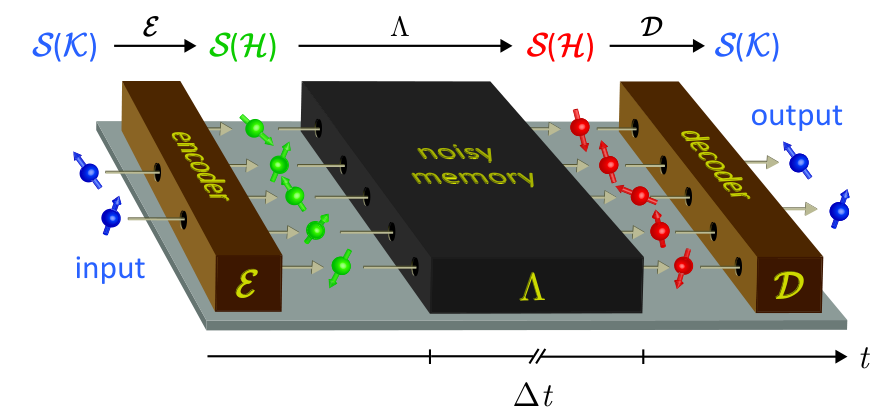
An error-correcting code for a channel $\Lambda$ consists of an encoding $\mathcal{E}$ , which is applied before the channel, and a decoding $\mathcal{D}$ , which is applied after the channel (see the explanations in Figure 1). Together, these devices form an error-corrected quantum memory for a smaller system, implementing a channel

\displaystyle\mathcal{D}\circ\Lambda\circ\mathcal{E}:\mathcal{S}(\mathcal{K})\rightarrow\mathcal{S}(\mathcal{K})\,,

(4)

where $\mathcal{K}$ is the Hilbert space of the smaller system and where $\circ$ denotes the composition of maps. Instead of evaluating the quantity (3) for the channel $\Lambda$ directly, it should be evaluated for such a corrected channel $\mathcal{D}\circ\Lambda\circ\mathcal{E}$ . A figure of merit for the usefulness of the quantum memory is then given by the size of the largest system $\mathcal{K}$ that can be stored in the memory using such an error-correcting code. This is identical to the largest subspace $\mathcal{H}^{\prime}\subseteq\mathcal{H}$ that is left approximately invariant by the memory. This is quantified by the one-shot quantum capacity $Q^{\varepsilon}(\Lambda)$ , defined by [4, 28]

\displaystyle Q^{\varepsilon}(\Lambda):=\max\{\log m\mid F_{\text{min}}(\Lambda,m)\geq 1-\varepsilon\}\,,

(5)

where

\displaystyle F_{\text{min}}(\Lambda,m):=\max_{\mathcal{H}^{\prime}\subseteq\mathcal{H}\atop\dim(\mathcal{H}^{\prime})=m}\max_{\mathcal{D}}\min_{|\phi\rangle\in\mathcal{H}^{\prime}}\langle\phi|(\mathcal{D}\circ\Lambda)(\phi)|\phi\rangle

(6)

and where the inner maximum is taken over all possible decoders $\mathcal{D}:\mathcal{S}(\mathcal{H})\rightarrow\mathcal{S}(\mathcal{H})$ . The logarithm in equation (5) (and in the rest of this article) is taken with respect to base 2, i.e. $\log\equiv\log_{2}$ . This way, the one-shot quantum capacity corresponds to the maximal number of qubits that can be stored and retrieved with a fidelity of at least $1-\varepsilon$ using the best possible error correcting code.

The one-shot quantum capacity tells us strictly more than the asymptotic quantum capacity, in the sense that the latter can be obtained from the former:

\displaystyle Q(\Lambda)=\lim_{\varepsilon\to 0}\lim_{N\to\infty}\frac{1}{N}Q^{\varepsilon}(\Lambda^{\otimes N})\,.

(7)

The asymptotic quantum capacity is the number of qubits that can be transmitted or stored per use of a device with asymptotically vanishing error, in the limit where it is used infinitely often under the i.i.d. assumption. Therefore, it is an asymptotic rate, while the one-shot quantum capacity is the total number of qubits that can be transmitted or stored in a single use of a (possibly non-tensor product) channel, allowing some error $\varepsilon\geq 0$ .

One-shot quantum capacity estimation

Protocol parameter

$\bullet$

$N\in\mathbb{N}$ , even: total number of qubits

The protocol

$\bullet$

Alice chooses $s\in\{0,1\}^{N}$ and $b\in\{X,Z\}^{N}_{N/2}$ fully at random and communicates them to Bob, where

$\displaystyle\{X,Z\}^{N}_{N/2}=\left\{b\in\{X,Z\}^{N}\,\middle|\,\parbox{71.13188pt}{X, Z { each occur $N/2$ times in $b$}}\right\}\,.$
$\bullet$

For each qubit slot $i=1,\ldots,N$ of the channel, Alice prepares a test qubit $i$ in the state $s_{i}$ with respect to basis $b_{i}\in\{X,Z\}$ and sends it through the channel to Bob.
$\bullet$

For each qubit $i=1,\ldots,N$ that Bob receives, he measures test qubit $i$ in the basis $b_{i}$ and records the outcome $s^{\prime}_{i}\in\{0,1\}$ .

\bullet

Bob determine the error rates

\displaystyle e_{x}=\frac{2}{N}\sum_{i\in I_{X}}s_{i}\oplus s^{\prime}_{i}\,,\qquad e_{z}=\frac{2}{N}\sum_{i\in I_{Z}}s_{i}\oplus s^{\prime}_{i}\,,

where

		$\displaystyle I_{X}=\{i\in\{1,\ldots,N\}\mid b_{i}=X\}\,,$
		$\displaystyle I_{Z}=\{i\in\{1,\ldots,N\}\mid b_{i}=Z\}\,.$

$\bullet$

Knowing the two error rates $e_{x}$ and $e_{z}$ , Bob determines a lower bound on the one-shot quantum capacity according to Theorem 1.

Protocol 1: The estimation protocol.

One-shot quantum capacity estimation

Now that the one-shot quantum capacity is identified as the relevant figure of merit for quantum memory and communication devices, the question is whether we can estimate this quantity for a given device. We answer this question in the affirmative for the case where $\Lambda$ is a channel that stores or communicates (arbitrarily many) qubits.

We present a simple protocol (see Protocol 1) that estimates the one-shot quantum capacity $Q^{\varepsilon}(\Lambda)$ for an $N$ -to- $N$ -qubit channel $\Lambda$ . Our protocol only requires the preparation and measurement of single qubit states in two bases. Specifically, even though it is known that the optimal encoder for a given channel $\Lambda$ may require the creation of a highly entangled state, no entanglement is required to execute our test. For simplicity, we assume here that $N$ is an even number (for more general cases, see Section D). The protocol does not make any assumption on whether the qubits are processed sequentially, as in communication devices, or in parallel, as in storage devices (potentially with correlated errors in both cases). The data collection of the protocol is very simple. Alice and Bob agree on two qubit bases $X$ and $Z$ . These two bases should be chosen to be “incompatible”, in the sense that the preparation quality $q$ , which is defined as

\displaystyle q=-\log\max_{i,j=0,1}\left\lvert{\langle i_{X}|j_{Z}\rangle}\right\rvert^{2}\,,

(8)

is as high as possible, where $|i_{X}\rangle$ and $|j_{Z}\rangle$ are eigenstates of $X$ and $Z$ , respectively. In the ideal case, where the two bases $X$ and $Z$ are mutually unbiased bases (MUBs), such as the Pauli- $X$ and $Z$ basis, it holds that $q=1$ . Our protocol can be seen as exploiting the idea that the ability to transmit information in two complementary bases relates to a channel’s ability to convey (quantum) information [21, 5], which we show holds even with correlated noise. We remark that Pauli- $X$ and $Z$ basis have also been used to estimate the process fidelity of a quantum operation [14, 24] in the i.i.d. case, which however we are precisely trying to avoid here.

The bound for the capacity estimate is a function of the number of qubits $N$ , the preparation quality $q$ , the maximally allowed decoding error probability $\varepsilon$ of $Q^{\varepsilon}(\Lambda)$ , the two measured error rates $e_{x}$ and $e_{z}$ , and some probability $p$ that quantifies the typicality of the protocol run (we will discuss this parameter in the Discussion section). More precisely, the bound is given as follows.

Theorem \@upn1 :

Let $N\in\mathbb{N}_{+}$ be an even number, let $e_{x}$ and $e_{z}$ be error rates determined in a run of Protocol 1 where the used bases $X$ and $Z$ had a preparation quality of $q$ (see equation (8) above). Then, for every $\varepsilon>0$ and for every $p\in[0,1)$ , it holds that

$\bullet$

either, the probability that at least one error rate exceeds $e_{x}$ or $e_{z}$ , respectively, was higher than $p$ ,
$\bullet$

or the one-shot quantum capacity of the $N$ -qubit channel $\Lambda$ is bounded by

where $h$ is the binary entropy function

\displaystyle h(x):=-x\log(x)-(1-x)\log(1-x)

(10)

and $\mu$ and $\kappa$ are given by

\displaystyle\mu=\sqrt{\frac{N+2}{N^{2}}\ln\left(\frac{3+\frac{5}{\sqrt{1-p}}}{\sqrt{\varepsilon/2}-\eta}\right)}\,,\quad\kappa=2\left(\frac{3+\frac{5}{\sqrt{1-p}}}{\sqrt{\varepsilon/2}-\eta}\right)^{2}\,.

(11)

In the asymptotic limit where $N\to\infty$ , the bound on the right hand side of inequality () converges to $N(q-h(e_{x})-h(e_{z}))$ . All the other terms can be seen as correction terms that account for finite-size effects. We will discuss this in more detail in the Discussion section below.

One-shot capacity verification

Protocol 1 above estimates how much quantum information can be stored in a quantum memory device. This is of great use when the task is to figure out whether a device is potentially useful as a quantum memory device. When eventually, an error-correcting code is implemented, the corrected memory might be used without further testing.

In some cases, however, one wants to implement the memory with a means to verify its quality while using it. For example, one may suspect the quality of the memory to diminish (say, due to damage or overuse). In that case, the capacity estimation that was made before the implementation of the error-correcting code may no longer be valid. A method to verify that the quality of the memory is good enough for the implemented code may be required whenever it is used. Protocol 2 shows such a verification protocol.

One-shot quantum capacity verification

Protocol parameters

$\bullet$

$N\in\mathbb{N}$ : number of data qubits
$\bullet$

$e_{x},e_{z}\in[0,1]$ : tolerated error rate in $X$ , $Z$

The protocol

\bullet

Alice chooses $s\in\{0,1\}^{3N}$ and $b\in\{X,Z,D\}^{3N}_{N}$ fully at random and communicates them to Bob, where

\displaystyle\{X,Z,D\}^{3N}_{N}=\left\{b\in\{X,Z,D\}^{3N}\,\middle|\,\parbox{42.67912pt}{\raggedright$X$, $Z$, $D$ { occur $N$ times in $b$}\@add@raggedright}\right\}.

$\bullet$

For each qubit slot $i=1,\ldots,{3N}$ of the channel, if $b_{i}\in\{X,Z\}$ , Alice prepares a test qubit $i$ in the state $s_{i}$ with respect to basis $b_{i}\in\{X,Z\}$ and sends it through the channel to Bob. If $b_{i}=D$ , Alice uses the slot for a data qubit.
$\bullet$

For each qubit $i=1,\ldots,{3N}$ that Bob receives, if $b_{i}\in\{X,Z\}$ , Bob measures test qubit $i$ in the basis $b_{i}$ and records the outcome $s^{\prime}_{i}\in\{0,1\}$ . If $b_{i}=D$ , Bob leaves the data qubit untouched.

\bullet

They determine the error rates

\displaystyle\gamma=\frac{1}{N}\sum_{i\in I_{X}}s_{i}\oplus s^{\prime}_{i}\,,\qquad\lambda=\frac{1}{N}\sum_{i\in I_{Z}}s_{i}\oplus s^{\prime}_{i}\,,

where

		$\displaystyle I_{X}=\{i\in\{1,\ldots,{3N}\}\mid b_{i}=X\}\,,$
		$\displaystyle I_{Z}=\{i\in\{1,\ldots,{3N}\}\mid b_{i}=Z\}\,.$

If $\gamma\leq e_{x}$ and $\lambda\leq e_{z}$ , they continue with the conclusion below. Otherwise, they abort the protocol.

$\bullet$

They conclude that the one-shot quantum capacity of the channel $\Lambda$ on the $N$ data qubits is bounded as in Theorem 2.

Protocol 2: The verification protocol.

The protocol assumes that Alice holds $N$ data qubits that she wants to send to Bob in a way that allows her to verify the quality of the transmission. To this end, she uses a channel for $3N$ qubits and places her $N$ data qubits in random slots of this channel. The other $2N$ slots are used for test qubits, half of which are prepared and measured in the $X$ -basis and half of which are prepared and measured in the $Z$ -basis (just as in the estimation protocol), while Alice and Bob leave the data qubits untouched. The error rates on the test bits allows to infer a bound on the capacity of the channel on the data qubits. This is shown in Figure 9.

(a) inference structure of the estimation protocol

(b) inference structure of the verification protocol

Figure 2: Comparison of the inference structures of the two protocols. (a) In the estimation protocol, all qubits are test qubits, and the goal is to estimate the capacity for the channel on all qubits. (b) In the verification protocol, one third of the qubits are data qubits that are left untouched. The remaining

2N

qubits are test qubits, whose error rates allow to bound the capacity of the channel on the

N

data qubits.

For this protocol, we denote the measured error rate in $X$ by $\gamma$ and the measured error rate in $Z$ by $\lambda$ . Bob checks whether these error rates exceed some tolerated values $e_{x}$ and $e_{z}$ , respectively, which has been specified before the protocol run. If one or both error rates exceed the tolerated value, the protocol aborts because the transmission quality is considered too low. If both error rates are below their tolerated value, Bob concludes that the transmission was of high quality, in the sense that the channel on the data qubits had a high one-shot quantum capacity. This is stated more precisely in the following theorem.

Theorem \@upn2 :

Let $N\in\mathbb{N}_{+}$ , let $e_{x}$ , $e_{z}\in[0,1]$ . Assume that Protocol 2 is run successfully without abortion, where the used bases $X$ and $Z$ had a preparation quality of $q$ . Then, for every $\varepsilon>0$ and for every $p\in[0,1)$ , it holds that

$\bullet$

either, the probability that the protocol aborts was higher than $p$ ,
$\bullet$

or the one-shot quantum capacity of the channel $\Lambda$ on the $N$ data qubits is bounded by inequality (), where $\kappa$ is as in equation (11) and where $\mu$ is given by

\displaystyle\mu=\sqrt{\frac{2(N+1)}{N^{2}}\ln\left(\frac{3+\frac{5}{\sqrt{1-p}}}{\sqrt{\varepsilon/2}-\eta}\right)}\,.

(12)

The bound for the verification protocol looks formally almost identical to the one for the estimation protocol, but there are three differences. Firstly, the function $\mu$ has a different dependence on $N$ , which is a consequence of the different structure of the protocol as explained in Figure 2. Secondly, the error rates $e_{x}$ and $e_{z}$ are preset accepted error rates instead of calculated error rates from data, and the bound holds when the measured rates are below those preset values. Thirdly, the probability $p$ in the bound is the abort probability of the protocol. We will say more about this probability in the Discussion section.

Discussion

In this section, we shall discuss our bound as a bound on the rate $\frac{1}{N}Q^{\varepsilon}(\Lambda)$ , which quantifies the amount of quantum information that can be sent per qubit. This has the advantage that it makes comparisons easier. To discuss our bound on the capacity rate, we have plotted its value as a function of $N$ in Figure 3. We plotted the bound for the estimation protocol, but qualitatively, the bound for the verification protocol behaves identically, so our discussion applies to both protocols.

(a) for different decoding error probabilities

\varepsilon

(b) for different error rates

e_{x}

and

e_{z}

Figure 3: Bound on the rate for the capacity estimation protocol as a function of the number of qubits. This figure shows the bound on the one-shot quantum capacity for the estimation protocol expressed as a rate, that is, the right hand side of inequality () divided by the number of qubits

N

. The plots show the bound as a function of

N

with the parameters as

q=1

, and

p=1/2

. (a) We plotted the bound for fixed error rates

e_{x}=e_{z}=5\%

for a few different values of

\varepsilon

in order to visualize the dependence on the decoding error probability. The lower the allowed decoding error probability

\varepsilon

is set, the higher the number of qubits needs to be in order to get a positive bound on the rate (note that the

N

-axis is logarithmic). In the asymptotic limit

N\to\infty

, the bound converges to

q-h(e_{x})-h(e_{z})

. If

q=1

, this coincides exactly with the (asymptotic) capacity for some important classes of channels, such as depolarizing channels. This shows that our bound is asymptotically optimal, and therefore, improvements are only possible in the finite-size correction terms. (b) To see the dependence on the error rates, we plotted our bound for a fixed value of

\varepsilon=10^{-6}

for a few different values of

e_{x}

and

e_{z}

. The higher the error rate, the higher the number of qubits needs to be in order to achieve a positive rate. For every pair of error rates

e_{x}

and

e_{z}

, the bound is monotonically increasing in

N

and converges to

q-h(e_{x})-h(e_{z})

. Therefore, the bound can only be positive when

q-h(e_{x})-h(e_{z})

is positive, which yields an easy criterion for the potential usefulness of a channel with known error rates (although the full version of the bound with the correction terms is not hard to evaluate either).

Example: Dephasing channel. In order to assess the strength of our bound, it is helpful consider some example channels. A particularly insightful example is the case where the channel $\Lambda$ is given by $N$ independent copies of a dephasing channel of strength $\alpha\in[0,1]$ , that is,

\displaystyle\Lambda=\Lambda_{D}^{\otimes N}\,,\quad\Lambda_{D}(\rho):\rho\mapsto\left(1-\frac{\alpha}{2}\right)\rho+\frac{\alpha}{2}\sigma\rho\sigma\,,

(13)

where $\sigma$ denotes one of the qubit Pauli operators with respect to some basis. Of particular interest is the case where the dephasing happens with respect to one of the two bases $X$ or $Z$ in which Alice and Bob prepare and measure the test qubits. Let us assume that $\sigma=\sigma_{Z}$ . In order to see what happens when our estimation protocol is used in this case, we could simulate a protocol run and see what bound on the one-shot quantum capacity would be obtained. However, the estimation protocol does essentially nothing but determine the two error rates $e_{x}$ and $e_{z}$ . The expected values of these rates can be readily obtained from equation (13). The error rate $e_{z}$ vanishes, because dephasing in the $Z$ -basis leaves the $Z$ -diagonal invariant. In the $X$ -basis the bits are left invariant with probability $1-\alpha/2$ , and flipped with probability $\alpha/2$ , so asymptotically $e_{x}=\alpha/2$ . Hence, for the dephasing channel, the estimation protocol is expected to yield the bound in inequality () with $e_{z}=0$ and $e_{x}=\alpha/2$ .

Asymptotic tightness of the bound. As one can see in Figure 3, the bound on the one-shot quantum capacity, expressed as a rate, converges to $q-h(e_{x})-h(e_{z})$ , which in the case of the dephasing channel is given by $q-h(\alpha/2)$ . If we additionally assume that the bases $X$ and $Z$ are mutually unbiased (as are Pauli- $X$ and $Z$ ), this is equal to $1-h(\alpha/2)$ . This is precisely the (asymptotic) quantum capacity of the dephasing channel. This means that our bound on the one-shot quantum capacity is asymptotically tight; if our bound can be improved, then only in the finite-size correction terms. In particular, our bound cannot be improved by a constant factor. Since most estimates that enter the derivation of the bound are of the same type as the estimates used in modern security proofs of QKD [30], any possible improvements of the QKD security bounds would also lead to an improvement of our bound on the one-shot quantum capacity (if there is any). In this sense, our bound is essentially as tight as the corresponding security bounds for QKD in the finite regime.

Measurement calibration. Above, we have assumed that Alice and Bob were very lucky: they set up their bases $X$ and $Z$ such that one of them is exactly aligned with the dephasing basis, and therefore optimally exploited the asymmetry of the channel. In general, since they do not know the channel whose capacity they estimate, they do not know about the direction of the asymmetry. Instead, they have to calibrate their devices by trying out several pairs of bases until they find one with low error rates. Otherwise, the bound on the one-shot quantum capacity that they infer is suboptimal. It is an interesting open question how such a calibration can be optimized.

Example: Fully depolarizing channel. Another insightful example is the case where $\Lambda$ is given by the channel which outputs the fully mixed state of $N$ qubits, independently of the input state. The capacity of this channel is zero, yet with probability $2^{-N}$ , Alice and Bob measure error rates $e_{x}=e_{z}=0$ . One may think that these vanishing error rates lead to a highly positive bound on the capacity, but this is not the case. As one can read in Theorem 1 and Theorem 2, the bound depends on a probability $p$ , and the term $1-p$ corresponds precisely to the probability of such an unlikely case. In fact, for $1-p=2^{-N}$ , the bound is never positive. This example shows that in the one-shot regime, a meaningful capacity estimation can only be made under the assumption that the observed data is not extremely untypical for the channel. However, this is only a problem for very low values of $N$ : thanks to the natural logarithm in $\mu$ (see equation (11) above), the concern reduces to untypical events with an exponentially (in $N$ ) small probability. For reasonable numbers of $N$ , the influence of $p$ on the bound is negligible, except for extremely low values of $1-p$ . For more information on this probability, see Section D. We note that this issue is not only given in our context of capacity estimation, but in all statistical tests on a finite sample, including quantum key distribution.

(a) plot for each of the three storage times

(b) zoomed-in plot for

\Delta t=$300\text{\,}\mathrm{ns}$

Figure 4: Bound on the rate for the experimental data as a function of

\varepsilon

. This figure shows the bound on the one-shot quantum capacity rate for the data gained in the transmon qubit. We pick

p=1/2

, and use

q=0.9

as preparation quality to account for the experimental imperfections. (a) The experiment was carried out three times with different storage times

\Delta t

, for each of which we plotted the bound resulting from the estimation protocol as a function of the decoding error probability

\varepsilon

. Since the number of qubit preparations and measurements was high (

N=$1.04\text{\times}{10}^{6}$

), the dependence on

\varepsilon

is rather small. (b) For a better visibility of the

\varepsilon

-dependence, we show the plot for the shortest storage time separately and more zoomed-in in the direction of the bound.

Experiment. We demonstrate the use of this protocol by implementing it on a Transmon qubit. The experiment is performed on qubit $A_{\mathrm{T}}$ previously reported on in [23]. We measure a relaxation time of $T_{1}=$18.5(\pm 0.6)\text{\,}\mathrm{\SIUnitSymbolMicro s}$$ and a Ramsey dephasing time of $T_{2}^{\star}=$3.8(\pm 0.3)\text{\,}\mathrm{\SIUnitSymbolMicro s}$$ before performing the experiment. Readout of the qubit state is performed by probing the readout resonator with a microwave tone. The resulting transients are amplified using a TWPA [16] at the front end of the amplification chain. This results in a readout fidelity $F_{\mathrm{RO}}=1-({p_{01}+p_{10}})/{2}=98.0\%$ , where $p_{01}$ ( $p_{10}$ ) is the probability of declaring state 1 (0) when the input state was $|0\rangle$ ( $|1\rangle$ ) respectively. The qubit state is controlled using resonant microwave pulses.

The experiment implements Protocol 1 to estimate the capacity of the idling operation $I(\tau)$ . We do this by generating 8000 pairs of random numbers corresponding to the bases $b\in\{X,Z\}$ and states $s\in\{0,1\}$ . These are then used to generate pulse sequences that rotate $|0\rangle$ to the required state, and wait for a time $\tau$ before measuring the qubit in the $Z$ -basis and declaring a state. If the required state was in the $X$ basis, a recovery pulse is applied that rotates the state to the $Z$ basis before it is read out. This protocol is repeated 130 times, with a distinct randomization for each repetition, yielding a total of $N=$1.04\text{\times}{10}^{6}$$ measurement outcomes in approximately one and a half hours.

(a) asymptotic rate bound for error rates on segments

(b) bound for aborted measurement sequence

Figure 5: Error fluctuations across the measurements. Here we visualize the statistical fluctuations in the measurement outcomes over the course of the transmon qubit experiment. (a) For the experiment with

\Delta t=$300\text{\,}\mathrm{ns}$

, we split up the

N=$1.04\text{\times}{10}^{6}$

sequential measurement outcomes into equally large and chronologically ordered segments and calculate the error rates

e_{x}

and

e_{z}

on each segment. For a meaningful and comparable quantity for comparison, we calculate the asymptotic bound

q-h(e_{x})-h(e_{z})

for each of segment with

q=0.9

, that is, the bound on the capacity rate that would be obtained if infinitely many measurements with the error rates as on the respective segments would be measured. As expected, the fluctuations decrease with the number of segments, or in other words, the larger the segments, the smaller the differences between them. Note that in contrast to all other plots, this is a linear plot. (b) For a glimpse on the cumulative effect of the fluctuations, we set 1000 logarithmically distributed “break points” and calculate the bound as if the experiment ended at each of those points where

q=0.9

\varepsilon=10^{-6}

, and we pick

p=1/2

. The resulting plot is to be compared with the plots in Figure 3. The fluctuations that make the curve deviate from a smooth curve come from the fact that the measured error rates are not constant throughout the experiment, indicating that the noise affecting the transmon qubit is indeed unlikely to correspond to an i.i.d. process.

Other open questions. Our result assumes that the system on which the channel acts is composed of qubits. An interesting open question is whether this restriction can be removed and an analogous bound can be derived for channels of arbitrary dimension and composition.

It would also be interesting to see our bound extended to continuous variable systems. There are many tools already available [11, 10, 3, 2] that may be useful to perform such an analysis, but it remains to be determined how exactly they can be applied to such systems.

Methods

To prove the bound on the one-shot quantum capacity, we combine several results. Firstly, as we recapitulate in more detail in Section B, it has been shown that the one-shot quantum capacity is bounded by the one-shot capacity of entanglement transmission $Q_{\textnormal{ent}}^{\varepsilon}(\Lambda)$ [1]. More precisely, it holds that for every channel $\Lambda$ and for every $\varepsilon>0$ [4],

\displaystyle Q^{\varepsilon}(\Lambda)\geq Q_{\textnormal{ent}}^{\varepsilon/2}(\Lambda)-1\,.

(14)

The one-shot capacity of entanglement transmission, in turn, has been proved to be bounded by the smooth min-entropy $H_{\textnormal{min}}^{\varepsilon}(A|E)_{\rho}$ , which is defined by

\displaystyle H_{\textnormal{min}}^{\varepsilon}(A|B)_{\rho}:=\max_{\rho^{\prime}\in B^{\varepsilon}(\rho)}H_{\textnormal{min}}(A|B)_{\rho^{\prime}}\,,

(15)

where

\displaystyle H_{\textnormal{min}}(A|B)_{\rho}:=\max_{\sigma_{B}}\sup\{\lambda\in\mathbb{R}\mid\rho_{AB}\leq 2^{-\lambda}I_{A}\otimes\sigma_{B}\}\,.

(16)

It has been shown that [4, 17, 28]

\displaystyle Q^{\varepsilon}_{\text{ent}}(\Lambda)\geq\sup_{\eta\in(0,\sqrt{\varepsilon})}\left(H_{\textnormal{min}}^{\sqrt{\varepsilon}-\eta}(A|E)_{\rho}-4\log\frac{1}{\eta}-1\right)\,,

(17)

Here, the smooth min-entropy is evaluated for the state

\displaystyle\rho_{AE}=(I_{A}\otimes\Lambda^{c}_{A^{\prime}\rightarrow E})(\Phi_{AA^{\prime}})\,,

(18)

where $\Phi_{AA^{\prime}}$ is a maximally entangled state over the input system $A^{\prime}$ and a copy $A$ of it, and where $\Lambda^{c}_{A^{\prime}\rightarrow E}$ is the complementary channel of the channel $\Lambda_{A^{\prime}\rightarrow B}$ . The system $E$ is the environment of the channel (see [33, 28] and Section B for more details). Taking together the results (14) and (17), we get that for all $\varepsilon>0$ ,

\displaystyle Q^{\varepsilon}(\Lambda)\geq\sup_{\eta\in(0,\sqrt{\varepsilon/2})}\left(H_{\textnormal{min}}^{\sqrt{\varepsilon/2}-\eta}(A|E)_{\rho}-4\log\frac{1}{\eta}-2\right)\,.

(19)

Therefore, the min-entropy bounds the one-shot quantum capacity.

Estimating the min-entropy has been a subject of intense research in quantum key distribution (QKD). However, min-entropy estimation protocols in QKD cannot be directly applied here, because they estimate the min-entropy $H_{\textnormal{min}}^{\varepsilon}(X|E)$ for classical information $X$ , while in the bound (17), the system $A$ holds quantum information. We bridge this gap: as our main technical contribution, we show in Section C that for a system $A$ that is composed of qubits, it holds that for every $\varepsilon>0$ and every $\varepsilon^{\prime},\varepsilon^{\prime\prime}\geq 0$ ,

		$\displaystyle H_{\text{min}}^{3\varepsilon+\varepsilon^{\prime}+4\varepsilon^{\prime\prime}}(A\|E)_{\rho}$
		$\displaystyle\quad\geq Nq-\left(H_{\text{max}}^{\varepsilon^{\prime\prime}}(X\|B)_{\rho}+H_{\text{max}}^{\varepsilon^{\prime}}(Z\|B)_{\rho}\right)-2\log\frac{2}{\varepsilon^{2}}\,.$		(20)

Inequality (20) reduces estimating the min-entropy of quantum information $A$ to estimating the max-entropy of measurement outcomes $X$ and $Z$ on the system $A$ .

We prove inequality (20) using three main ingredients. Firstly, we use an uncertainty relation for the smooth min- and max-entropies [31]. Secondly, we use a duality relation for the smooth min- and max-entropies [15, 29]. These two ingredients were also used in modern security proofs of quantum key distribution [30]. We combine these two tools with a third tool, namely a chain rule theorem for the smooth max-entropy [32] to arrive at the bound in inequality (20).

Given inequalities (17) and (20), all we are left to do is to devise a protocol that estimates the max-entropies of $X$ and $Z$ given Bob’s quantum information $B$ . Here we can make use of protocols in quantum key distribution that estimate exactly such a quantity. We show in Section D how two such protocols (one for the max-entropy of $X$ and one for the max-entropy of $Z$ ) can be combined into one protocol, which estimates both quantities simultaneously. The resulting protocol, which we presented in two versions, is given by Protocol 1 and Protocol 2 in the Results section. Our bound on the one-shot quantum capacity of the channel, inequality (), is obtained by combining inequalities (14) and (17) with these max-entropy estimation techniques.

Acknowledgements

We thank the Leo DiCarlo group (incl. MAR) at QuTech for providing test data for a superconducting qubit. We also thank Mario Berta, Thinh Le Phuc and Jeremy Ribeiro for insightful discussions, and Julia Cramer for helpful comments on an earlier version of this manuscript. CP, AM, MT and SW were supported by MOE Tier 3A grant ”Randomness from quantum processes”, NRF CRP ”Space-based QKD”. SW was also supported by STW, Netherlands, an NWO VIDI Grant, and an ERC Starting Grant. MAR was supported by an ERC Synergy grant.

References

[1] H. Barnum, E. Knill, and M. A. Nielsen. On quantum fidelities and channel capacities. IEEE Trans. Inf. Theory, 46(4):1317–1329, 2000.
[2] M. Berta, M. Christandl, F. Furrer, V. B. Scholz, and M. Tomamichel. Continuous variable entropic uncertainty relations in the presence of quantum memory. arXiv:1308.4527, 2013.
[3] M. Berta, F. Furrer, and V. B. Scholz. The smooth entropy formalism for von neumann algebras. Journal of Mathematical Physics, 57(015213), 2016.
[4] F. Buscemi and N. Datta. The quantum capacity of channels with arbitrarily correlated noise. IEEE Trans. Inf. Theory, 56(3):1447–1460, 2010.
[5] M. Christandl and A. Winter. Uncertainty, monogamy, and locking of quantum correlations. IEEE Trans. Inf. Theory, 51(9):3159–3165, 2005.
[6] I. L. Chuang and M. A. Nielsen. Prescription for experimental determination of the dynamics of a quantum black box. J. Mod. Opt., 44(11–12):2455–2467, 1997.
[7] G. M. D’Ariano. Characterization of Quantum Devices. Springer-Verlag Berlin Heidelberg, 2004.
[8] P. Faist and R. Renner. Practical and reliable error bars in quantum tomography. Phys. Rev. Lett., 117:010404, 2016.
[9] C. Ferrie and R. Blume-Kohout. Minimax quantum tomography: Estimators and relative entropy bounds. Phys. Rev. Lett., 116:090407, 2016.
[10] F. Furrer, J. Aberg, and R. Renner. Min- and max-entropy in infinite dimensions. Communications in Mathematical Physics, 306(1):165–186, 2011.
[11] F. Furrer, T. Franz, M. Berta, A. Leverrier, V. B. Scholz, M. Tomamichel, and R. F. Werner. Continuous variable quantum key distribution: Finite-key analysis of composable security against coherent attacks. Phys. Rev. Lett., 109:100502, 2012.
[12] D. Greenbaum. Introduction to quantum gate set tomography. 2015.
[13] E. Greene and J. A. Wellner. Exponential bounds for the hypergeometric distribution, 2015.
[14] H. F. Hofmann. Complementary classical fidelities as an efficient criterion for the evaluation of experimentally realized quantum operations. Phys. Rev. Lett., 94:160504, 2005.
[15] R. König, R. Renner, and C. Schaffner. The operational meaning of min- and max-entropy. IEEE Trans. Inf. Theory, 55(9):4337–4347, 2009.
[16] C. Macklin, K. O’Brien, D. Hover, M. E. Schwartz, V. Bolkhovsky, X. Zhang, W. D. Oliver, and I. Siddiqi. A near-quantum-limited Josephson traveling-wave parametric amplifier. Science, (September):1–8, sep 2015.
[17] C. Morgan and A. Winter. Pretty strong converse for the quantum capacity of degradable channels. IEEE Trans. Inf. Theory, 60(1):317–333, Jan 2014.
[18] M. A. Nielsen and I. L. Chuang. Quantum Computation and Quantum Information. Cambridge University Press, 2000.
[19] C. Pfister. Decoherence estimation in Quantum Theory and Beyond. PhD thesis, 2016.
[20] C. Pfister, N. Lütkenhaus, S. Wehner, and P. J. Coles. Sifting attacks in finite-size quantum key distribution. New J. Phys., 18(5):053001, 2016.
[21] J. M. Renes and J.-C. Boileau. Conjectured strong complementary information tradeoff. Phys. Rev. Lett., 103:020402, 2009.
[22] R. Renner. Security of Quantum Key Distribution. PhD thesis, ETH Zürich, 2005.
[23] D. Ristè, S. Poletto, M. Z. Huang, A. Bruno, V. Vesterinen, O. P. Saira, and L. DiCarlo. Detecting bit-flip errors in a logical qubit using stabilizer measurements. Nat. Commun., 6, 2015.
[24] M. Sedlák and J. Fiuráŝek. Generalized hofmann quantum process fidelity bounds for quantum filters. Phys. Rev. A, 93:042316, 2016.
[25] R. J. Serfling. Probability inequalities for the sum in sampling without replacement. Ann. Stat., 2(1):39–48, 1974.
[26] W. F. Stinespring. Positive functions on C*-algebras. Proc. Amer. Math. Soc., 6(2), 1955.
[27] M. Tomamichel. A Framework for Non-Asymptotic Quantum Information Theory. PhD thesis, 2012.
[28] M. Tomamichel, M. Berta, and J. M. Renes. Quantum coding with finite resources. Nat. Comm., 7(11419), 2016.
[29] M. Tomamichel, R. Colbeck, and R. Renner. Duality between smooth min- and max-entropies. IEEE Trans. Inf. Theory, 56(9):4674–4681, 2010.
[30] M. Tomamichel, C. Lim, N. Gisin, and R. Renner. Tight finite-key analysis for quantum cryptography. Nat. Commun., 3(634), 2012.
[31] M. Tomamichel and R. Renner. Uncertainty relation for smooth entropies. Phys. Rev. Lett., 106(11):110506, 2011.
[32] A. Vitanov, F. Dupuis, M. Tomamichel, and R. Renner. Chain rules for smooth min- and max-entropies. IEEE Trans. Inf. Theory, 59(5):2603–2612, 2013.
[33] M. Wilde. Quantum Information Theory. Cambridge University Press, 2013.

Appendix A Mathematical preliminaries and conventions

In appendix A, we recapitulate some basic definitions. The material presented should not be seen as an introduction to the subject. We only state the definitions here to avoid ambiguity and to clarify our notation. The following definition clarifies our notation for operator spaces.

Definition \@upn3 (Operator spaces):

For a finite-dimensional complex inner product space $\mathcal{H}$ , we define the following sets of operators on $\mathcal{H}$ :

$\bullet$

$\textnormal{End}(\mathcal{H}):=\left\{L:\mathcal{H}\rightarrow\mathcal{H}\mid L\textnormal{ linear}\right\}$ , (endomorphisms on $\mathcal{H}$ )
$\bullet$

$\textnormal{Herm}(\mathcal{H}):=\left\{L\in\textnormal{End}(\mathcal{H})\mid L^{\dagger}=L\right\}$ , (Hermitian operators on $\mathcal{H}$ )
$\bullet$

$\mathcal{S}(\mathcal{H}):=\{\rho\in\textnormal{Herm}(\mathcal{H})\mid\rho\geq 0,\textnormal{tr}(\rho)=1\}$ , (states / density operators on $\mathcal{H}$ )
$\bullet$

$\mathcal{S}^{\leq}(\mathcal{H}):=\{\rho\in\textnormal{Herm}(\mathcal{H})\mid\rho\geq 0,\textnormal{tr}(\rho)\leq 1\}$ . (subnormalized states on $\mathcal{H}$ )

Next, we make some general conventions.

Conventions \@upn0 :

Throughout this document, we make use of the following conventions:

$\bullet$

$\log$ denotes the binary logarithm (base 2) and $\ln$ denotes the natural logarithm (base $e$ ).
$\bullet$

Quantum systems are assumed to be finite-dimensional, and the symbol $\mathcal{H}$ always denotes a finite-dimensional complex inner product space.
$\bullet$

A single subscript of $\mathcal{H}$ refers to the system associated with the space (for example, $\mathcal{H}_{A}$ is the space of system $A$ ).
$\bullet$

We use multiple subscripts of $\mathcal{H}$ to refer to a space of a joint system (for example, $\mathcal{H}_{AB}=\mathcal{H}_{A}\otimes\mathcal{H}_{B}$ ).
$\bullet$

For multipartite states, such as $\rho_{ABE}\in\mathcal{S}(\mathcal{H}_{ABE})$ , we denote its reduced states by according changes of the subscript, e.g. $\rho_{AE}:=\textnormal{tr}_{B}(\rho_{ABE})$ , $\rho_{A}:=\textnormal{tr}_{B}(\textnormal{tr}_{E}(\rho_{ABE}))$ .

The formal definition of a quantum channel goes as follows.

Definition \@upn4 (Quantum channel):

Let $A$ and $B$ be quantum systems.

\bullet

The identity channel on $A$ , denoted by $I_{A}$ , is the linear map

\displaystyle\begin{array}[]{cccc}I_{A}:&\textnormal{End}(\mathcal{H}_{A})&\rightarrow&\textnormal{End}(\mathcal{H}_{A})\\ &\rho_{A}&\mapsto&\rho_{A}\,.\end{array}

$\bullet$

A quantum channel from $A$ to $B$ is a linear map

$\displaystyle\Lambda:\textnormal{End}(\mathcal{H}_{A})\rightarrow\textnormal{End}(\mathcal{H}_{B})$ (23)

which is trace-preserving, i.e.

$\displaystyle\textnormal{tr}(\Lambda(\rho_{A}))=\textnormal{tr}(\rho_{A})\quad\Forall\rho_{A}\in\textnormal{End}(\mathcal{H}_{A})\,,$ (24)

and which is completely positive. That is, for any quantum system $E$ of any dimension $d_{E}\in\mathbb{N}_{+}$ , the map $\Lambda\otimes I_{E}$ is a positive map,

$\displaystyle(\Lambda\otimes I_{E})(\rho_{AE})\geq 0\quad\Forall\rho_{AE}\in\mathcal{H}_{AE}\,.$ (25)

Such a map is called a trace-preserving completely positive map (abbreviated as TPCPM).¹¹ 1 According to this definition, the terms “channel” and “TPCPM” are equivalent. In practice, the term channel is preferred when speaking of the evolution of a system in a physical sense, while the term TPCPM refers to the map as a mathematical object. However, this distinction is often not very strict.

In order to define the the one-shot quantum capacity of a channel and the smooth entropies of quantum channels below, we need to make use of some distance measures.

Definition \@upn5 (Distance measures):

On the above operator spaces, we define the following distance measures:

$\bullet$

The trace norm on $\textnormal{End}(\mathcal{H})$ is defined as $\left\lVert L\right\rVert_{1}=\textnormal{tr}\left(\sqrt{L^{\dagger}L}\right)$ .
$\bullet$

The trace distance on $\textnormal{End}(\mathcal{H})$ is defined as $D(\rho,\sigma):=\frac{1}{2}\left\lVert\rho-\sigma\right\rVert_{1}$ .
$\bullet$

The generalized fidelity [29] on $\mathcal{S}^{\leq}(\mathcal{H})$ is defined as $F(\rho,\sigma):=\left\|\sqrt{\rho}\sqrt{\sigma}\right\|_{1}+\sqrt{(1-\textnormal{tr}\rho)(1-\textnormal{tr}\sigma)}$ .
$\bullet$

The fidelity is given by the restriction of the generalized fidelity to $\mathcal{S}(\mathcal{H})$ , resulting in $F(\rho,\sigma)=\left\lVert\sqrt{\rho}\sqrt{\sigma}\right\rVert$ .
$\bullet$

The purified distance on $\mathcal{S}^{\leq}(\mathcal{H})$ is defined as $P(\rho,\sigma):=\sqrt{1-F(\rho,\sigma)^{2}}$ .
$\bullet$

The $\mathbf{\varepsilon}$ -ball around a subnormalized state $\rho\in\mathcal{S}^{\leq}(\mathcal{H})$ is given by $B^{\varepsilon}(\rho):=\{\rho^{\prime}\in\mathcal{S}^{\leq}(\mathcal{H})\mid P(\rho,\rho^{\prime})\leq\varepsilon\}$ .

Next, we define two kinds of one-shot capacities for quantum channels. There are (at least) two meaningful definitions of a capacity. In the i.i.d. scenario, these two capacities happen to coincide, and they are just referred to as the quantum capacity of a quantum channel. In the one-shot case, however, the two capacities are distinct, so it is not a priori clear which one should be chosen as the one-shot quantum capacity $Q^{\varepsilon}(\Lambda)$ . Here, we follow Buscemi and Datta [4], identifying the one-shot capacity of minimum output fidelity as the one-shot quantum capacity. More precisely, we define the following.

Definition \@upn6 (One-shot capacities):

Let $\Lambda:\textnormal{End}(\mathcal{H}_{A})\rightarrow\textnormal{End}(\mathcal{H}_{B})$ be a quantum channel, let $\varepsilon\geq 0$ .

\bullet

The one-shot capacity of minimum output fidelity $Q^{\varepsilon}(\Lambda)$ of the channel with respect to $\varepsilon$ , which we also call the one-shot quantum capacity of the channel, is defined as

\displaystyle Q^{\varepsilon}(\Lambda):=\max\{\log m\mid F_{\text{min}}(\Lambda,m)\geq 1-\varepsilon\}\,,

(26)

where

\displaystyle F_{\text{min}}(\Lambda,m):=\max_{\mathcal{H}_{A}^{\prime}\subseteq\mathcal{H}_{A}\atop\dim\left(\mathcal{H}_{A}^{\prime}\right)=m}\max_{\mathcal{D}}\min_{|\phi\rangle\in\mathcal{H}_{A}^{\prime}}\langle\phi|(\mathcal{D}\circ\Lambda)(\phi)|\phi\rangle\,.

(27)

The inner maximization ranges over all channels $\mathcal{D}:\textnormal{End}(\mathcal{H}_{B})\rightarrow\textnormal{End}(\mathcal{H}_{A})$ (decoding channels).

\bullet

The one-shot capacity of entanglement transmission $Q_{\textnormal{ent}}^{\varepsilon}(\Lambda)$ of the channel is defined as

\displaystyle Q_{\textnormal{ent}}^{\varepsilon}(\Lambda):=\max\{\log m\mid F_{\text{ent}}(\Lambda,m)\geq 1-\varepsilon\}\,,

(28)

where

\displaystyle F_{\text{ent}}(\Lambda,m):=\max_{\mathcal{H}_{M}\subseteq\mathcal{H}_{A}\atop\dim(\mathcal{H}_{M})=m}\max_{\mathcal{D}}\langle\Phi_{MM^{\prime}}|(\mathcal{D}\circ\Lambda)(\Phi_{MM^{\prime}})|\Phi_{MM^{\prime}}\rangle

The maximization over $\mathcal{D}$ is as above, and the state

\displaystyle|\Phi_{MM^{\prime}}\rangle=\frac{1}{\sqrt{\dim(\mathcal{H}_{M})}}\sum_{i=1}^{\dim(\mathcal{H}_{M})}\left(|i\rangle_{M}\otimes|i\rangle_{M^{\prime}}\right)

(29)

is a maximally entangled state on the subsystem $\mathcal{H}_{M}$ and a copy $\mathcal{H}_{M^{\prime}}$ of it.

Although these two capacities are distinct, we will see below that they are comparable in the sense that they bound each other (see inequality (34) below). It is important to note that in Definition 6, we follow the definitions in [4] and [28] by using the fidelity as the figure of merit. Other sources, such as [17], define the one-shot capacities with the trace distance as the figure of merit. This will have consequences in Section B, when a bound on $Q_{\textnormal{ent}}^{\varepsilon}(\Lambda)$ is converted from one definition to another (see inequality (41) below).

Now we define the (smooth) min- and max-entropy of a bipartite quantum state.

Definition \@upn7 (Min- and max-entropy):

Let $\rho_{AB}\in\mathcal{S}^{\leq}(\mathcal{H}_{AB})$ be a subnormalized bipartite state.

\bullet

The min-entropy of $A$ conditioned on $B$ for the state $\rho_{AB}$ is defined [22] as

\displaystyle H_{\textnormal{min}}(A|B)_{\rho}:=\max_{\sigma_{B}\in\mathcal{S}^{\leq}(\mathcal{H}_{B})}\sup\{\lambda\in\mathbb{R}\mid\rho_{AB}\leq 2^{-\lambda}I_{A}\otimes\sigma_{B}\}\,.

(30)

\bullet

The max-entropy of $A$ given $B$ for the state $\rho_{AB}$ is defined [15] as

\displaystyle H_{\textnormal{max}}(A|B)_{\rho}:=\max_{\sigma_{B}\in\mathcal{S}^{\leq}(\mathcal{H}_{B})}\log\left\|\sqrt{\rho_{AB}}\sqrt{I_{A}\otimes\sigma_{B}}\right\|^{2}_{1}\,.

(31)

Definition \@upn8 (Smooth min- and max-entropy):

Let $\rho_{AB}\in\mathcal{S}^{\leq}(\mathcal{H}_{AB})$ be a bipartite state and let $\varepsilon\geq 0$ .

\bullet

The $\varepsilon$ -smooth max-entropy of $A$ conditioned on $B$ is defined as

\displaystyle H_{\textnormal{max}}^{\varepsilon}(A|B)_{\rho}:=\min_{\rho^{\prime}\in B^{\varepsilon}(\rho)}H_{\textnormal{max}}(A|B)_{\rho^{\prime}}\,,

(32)

\bullet

The $\varepsilon$ -smooth min-entropy of $A$ conditioned on $B$ is defined as

\displaystyle H_{\textnormal{min}}^{\varepsilon}(A|B)_{\rho}:=\max_{\rho^{\prime}\in B^{\varepsilon}(\rho)}H_{\textnormal{min}}(A|B)_{\rho^{\prime}}\,.

(33)

For states that are defined on more systems than labeled in the entropy, the entropy is evaluated for the according reduced state. For example, given a state $\rho_{ABE}\in\mathcal{H}_{ABE}$ , the smooth min-entropy $H_{\textnormal{min}}^{\varepsilon}(A|E)_{\rho}$ is evaluated for $\rho_{AE}=\textnormal{tr}_{B}(\rho_{ABE})$ .

To avoid confusion with other sources that define the smooth min- and max-entropies, it is important to note two things.

$\bullet$

Firstly, the max-entropy, as we defined it in Definition 7, coincides with the Rényi entropy of order 1/2, whereas in some older sources, it was defined as the Rényi entropy of order 0 [22].
$\bullet$

Secondly, the smooth entropies, as we defined them in Definition 8, measure the distance in the purified distance, whereas in some older sources, it was defined with respect to the trace distance [22].

There are several reasons for making the definitions as we use them here. One important reason is that this way, the smooth min- and max-entropies satisfy a duality relation [29] that we will exploit in Section C (see Lemma 11).

Appendix B Background: Proof of the min-entropy bound on the one-shot quantum capacity

In appendix B, we explain the details of the min-entropy bound on the one-shot quantum capacity (inequality (17) of the main article) and show how it is derived. This is not a new result, but an application of results that are well-established in quantum information science, which we provide here for convenience of the reader.

As mentioned in the main article, as the first step in the derivation of inequality (17), we note that the one-shot quantum capacity $Q^{\varepsilon}(\Lambda)$ of a quantum channel $\Lambda$ can be lower-bounded by the one-shot capacity of entanglement transmission $Q_{\textnormal{ent}}^{\varepsilon}(\Lambda)$ . More precisely, Barnum, Knill and Nielsen [1] have shown that (here we use the form presented in [4])

\displaystyle\Forall\varepsilon>0:Q_{\textnormal{ent}}^{\varepsilon}(\Lambda)-1\leq Q^{2\varepsilon}(\Lambda)\leq Q_{\textnormal{ent}}^{4\varepsilon}(\Lambda)\,.

(34)

In particular,

\displaystyle\Forall\varepsilon>0:\quad Q^{\varepsilon}(\Lambda)\geq Q_{\textnormal{ent}}^{\varepsilon/2}(\Lambda)-1\,.

(35)

In the next step, we will bound $Q_{\textnormal{ent}}^{\varepsilon}(\Lambda)$ . Before we do that, it is helpful to extend our picture with the Stinespring dilation of the channel and a purification of the input state, as shown in Figures 6 and 7. Readers who are already familiar with these concepts may skip this part and continue reading below Figure 7.

Recapitulate the situation that we consider: we are given a quantum channel $\Lambda$ that takes a quantum system on Alice’s side as its input and outputs another quantum system on Bob’s side. It is helpful to give these input and output systems their own labels. We denote the input system on Alice’s side by $A^{\prime}$ and the output system on Bob’s side by $B$ (the reason for choosing $A^{\prime}$ instead of $A$ will become clear below). The situation is depicted in Figure 6(a).

(a) A channel

\Lambda

from

A^{\prime}

B

(b) Stinespring dilation of

\Lambda

from

A^{\prime}

BE

Figure 6: An arbitrary quantum channel

\Lambda

and its Stinespring dilation

V^{\Lambda}

. For every channel

\Lambda

from

A^{\prime}

B

, there is an isometry

V^{\Lambda}

such that

\Lambda(\rho_{A^{\prime}})=\textnormal{tr}(V^{\Lambda}\rho_{A^{\prime}}(V^{\Lambda})^{\dagger})

. Isometries have the important property that they map pure input states to pure output states. This will be important below, where we purify the input state

\rho_{A^{\prime}}

(see Figure 7).

For our purposes, it is useful to extend this picture. Mathematically speaking, a quantum channel is a trace-preserving completely positive map that maps density operators $\rho_{A^{\prime}}$ to density operators $\rho_{B}$ ,

\displaystyle\Lambda:\mathcal{S}(\mathcal{H}_{A^{\prime}})\rightarrow\mathcal{S}(\mathcal{H}_{B})\,.

(36)

The Stinespring dilation theorem [26] states that for every such completely positive map $\Lambda$ , there is a system $E$ of dimension $d_{E}\leq d_{A^{\prime}}^{2}$ and a linear isometry

\displaystyle V^{\Lambda}:\mathcal{H}_{A^{\prime}}\rightarrow\mathcal{H}_{B}\otimes\mathcal{H}_{E}

(37)

such that

\displaystyle\Lambda(\rho_{A^{\prime}})=\textnormal{tr}_{E}\left(V^{\Lambda}\rho_{A^{\prime}}\left(V^{\Lambda}\right)^{\dagger}\right)\,.

(38)

The extended picture is shown in Figure 6(b). The map $V^{\Lambda}$ is an isometric extension or Stinespring dilation of the channel $\Lambda$ , and is a standard tool in quantum information theory [33].

We extend this picture further using another standard tool in quantum information. The input state $\rho_{A^{\prime}}$ of the channel may not be a pure state but a mixed state. This is inconvenient, as many useful mathematical statements require the involved states to be pure. However, we can work around this by considering a purification of $\rho_{A^{\prime}}$ , that is, a system $A$ of dimension $d_{A}\leq d_{A^{\prime}}$ and a pure state $\rho_{AA^{\prime}}$ such that $\textnormal{tr}_{A}(\rho_{AA^{\prime}})=\rho_{A}^{\prime}$ . Every state has such a purification, but it is not unique [18]. Here, for every state $\rho_{A^{\prime}}$ , we consider a purification with $d_{A}=d_{A^{\prime}}$ , which is called the canonical purification $\psi_{AA^{\prime}}^{\rho}$ , and is given by $\psi_{AA^{\prime}}^{\rho}=|\psi^{\rho}\rangle\langle\psi^{\rho}|_{AA^{\prime}}$ , where

\displaystyle|\psi^{\rho}\rangle_{AA^{\prime}}=d_{A^{\prime}}\ \left(I_{A}\otimes\sqrt{\rho_{A^{\prime}}}\right)|\Phi\rangle_{AA^{\prime}}\,.

(39)

Here, $|\Phi_{AA^{\prime}}\rangle$ is the maximally entangled basis with respect to some bases $\{|i\rangle_{A}\}_{i}$ and $\{|i\rangle_{A^{\prime}}\}_{i}$ for $\mathcal{H}_{A}$ and $\mathcal{H}_{A^{\prime}}$ , respectively (their choice is irrelevant for what we consider),

\displaystyle|\Phi\rangle_{AA^{\prime}}=\sum_{i=1}^{d_{A^{\prime}}}\frac{1}{\sqrt{d_{A^{\prime}}}}|i\rangle_{A}\otimes|i\rangle_{A^{\prime}}\,.

(40)

By extending system $A^{\prime}$ to system $AA^{\prime}$ in this way, we arrive at the overall picture shown in Figure 7. After the channel $\Lambda$ acted on system $A^{\prime}$ , we not only consider the output system $B$ but the tripartite system $ABE$ , which is in a state $\rho_{ABE}$ . Since isometries map pure input states to pure output states, is is a pure state. This is the reason for this extension. It will allow us to apply the duality relation in Section C (see Lemma 11).

Figure 7: The fully purified diagram for a quantum channel. Since the input state

\psi_{AA^{\prime}}^{\rho}

is pure and

I_{A}\otimes V^{\Lambda}

is an isometry, the output state

\rho_{ABE}

is pure.

Now we are ready to proceed with the next step in the derivation of inequality (17). It turns out that the one-shot capacity of entanglement transmission $Q_{\textnormal{ent}}^{\varepsilon}(\Lambda)$ of the channel $\Lambda$ can be bounded by functions of the state $\rho_{ABE}$ that we described above. Buscemi and Datta [4] have shown that a lower bound on the one-shot capacity of entanglement transmission can be formulated in terms of a maximization of an entropic quantity. Subsequently, Morgan and Winter tightened this bound and translated it to an optimization of the smooth min-entropy of the state $\rho_{AE}=\textnormal{tr}_{B}(\rho_{ABE})$ [17]. Here we use this bound in the following form [28]:

\displaystyle\Forall\varepsilon>0:\quad Q^{\varepsilon}_{\text{ent}}(\Lambda)\geq\sup_{\eta\in(0,\sqrt{\varepsilon})}\sup_{\rho_{A^{\prime}}\in\mathcal{S}(\mathcal{H}_{A^{\prime}})}\left(H_{\textnormal{min}}^{\sqrt{\varepsilon}-\eta}(A|E)_{\rho}-4\log\frac{1}{\eta}-1\right)\,.

(41)

The square root in the smoothing parameter is a consequence of the fact that the bound (41) was derived through conversion from a bound where the figure of merit for entanglement transmission was the purified distance [17] instead of the fidelity [28].

Next, we drop the maximization over the state $\rho_{A^{\prime}}\in\mathcal{S}(\mathcal{H}_{A^{\prime}})$ by choosing the maximally mixed state $\rho_{A^{\prime}}=I_{A^{\prime}}/d_{A^{\prime}}$ . This way, we arrive at another lower bound:

\displaystyle\Forall\varepsilon>0:\quad Q^{\varepsilon}_{\text{ent}}(\Lambda)\geq\sup_{\eta\in(0,\sqrt{\varepsilon})}\left(H_{\textnormal{min}}^{\sqrt{\varepsilon}-\eta}(A|E)_{\rho}-4\log\frac{1}{\eta}-1\right)\,.

(42)

This corresponds to the case where the input state $\psi^{\rho}_{AA^{\prime}}$ in Figure 7 is given by the maximally entangled state $\Phi_{AA^{\prime}}$ (see equations (39) and (40) above). This is of particular importance for us because we can actually estimate $H_{\textnormal{min}}^{\varepsilon}(A|E)$ in that case (see Section D). Combining inequalities (35) and (42), we get the bound

\displaystyle\Forall\varepsilon>0:\quad Q^{\varepsilon}(\Lambda)\geq\sup_{\eta\in(0,\sqrt{\varepsilon/2})}\left(H_{\textnormal{min}}^{\sqrt{\varepsilon/2}-\eta}(A|E)_{\rho}-4\log\frac{1}{\eta}-2\right)\,.

(43)

Appendix C Result: Proof of the bound on the min-entropy

In Section B, we have seen that the one-shot quantum capacity $Q^{\varepsilon}(\Lambda)$ can be bounded in terms of the smooth min-entropy $H_{\textnormal{min}}^{\varepsilon}(A|E)$ of an appropriately defined state $\rho_{AE}$ . In this appendix, we prove that this min-entropy is bounded by the smooth max-entropies $H_{\textnormal{max}}^{\varepsilon}(X|B)$ and $H_{\textnormal{max}}^{\varepsilon}(Z|B)$ of measurement $X$ and $Z$ on $A$ . More precisely, we will show:

\displaystyle\Forall\varepsilon>0,\Forall\varepsilon^{\prime},\varepsilon^{\prime\prime}\geq 0:\quad H_{\text{min}}^{3\varepsilon+\varepsilon^{\prime}+4\varepsilon^{\prime\prime}}(A|E)_{\rho}\geq Nq-\left(H_{\text{max}}^{\varepsilon^{\prime\prime}}(X|B)_{\rho}+H_{\text{max}}^{\varepsilon^{\prime}}(Z|B)_{\rho}\right)-2\log\frac{2}{\varepsilon^{2}}

(44)

(see Theorem 15 below). Using this inequality, we will prove our bound on the one-shot quantum capacity in terms of the protocol parameters in Section D.

In the following, we will cite some lemmas that we will need for the proof of the bound (44). The most important ones are:

$\bullet$

an uncertainty relation for the smooth min- and max-entropies [31],
$\bullet$

a chain rule theorem for the smooth max-entropy [32] and
$\bullet$

a duality relation for the smooth min- and max-entropies [15, 29].

We start with the uncertainty relation for the smooth min- and max-entropies.

Lemma \@upn9 (Smooth min-max uncertainty):

Let $\rho_{ABE}\in\mathcal{S}(\mathcal{H}_{ABE})$ be a pure tripartite state where $A$ is an $N$ -qubit system, let $X=\{X_{0},X_{1}\}$ and $Z=\{Z_{0},Z_{1}\}$ be qubit POVMs. Consider the states $\rho_{XBE}$ and $\rho_{ZBE}$ that arise from measuring all of the $N$ qubits of system $A$ with respect to $X$ and $Z$ , respectively, and storing the outcomes in a classical register $X$ and $Z$ , respectively,

	$\displaystyle\rho_{XBE}$	$\displaystyle=\sum_{x\in\{0,1\}^{n}}P_{X}(x)\ \|x\rangle\langle x\|\otimes\rho_{BE}^{x}\,,$		(45)
	$\displaystyle\rho_{ZBE}$	$\displaystyle=\sum_{z\in\{0,1\}^{n}}P_{Z}(z)\ \|z\rangle\langle z\|\otimes\rho_{BE}^{z}\,.$		(46)

where

		$\displaystyle P_{X}(x)=\textnormal{tr}\left(\Pi_{X}(x)\rho_{A}\right)\,,$		(47)
		$\displaystyle\Pi_{X}(x)=\bigotimes_{i=1}^{n}X_{x_{i}}\quad\text{for }x=(x_{1},\ldots,x_{n})\in\{0,1\}^{n}\,,$		(48)
		$\displaystyle\rho^{x}_{BE}=\frac{\textnormal{tr}_{A}((\Pi_{X}(x)\otimes I_{BE})\rho_{ABE}(\Pi_{X}(x)\otimes I_{BE}))}{P_{X}(x)}\,,$		(49)

and analogously for $\rho_{ZBE}$ . Then for $\varepsilon\geq 0$ ,

\displaystyle H_{\textnormal{min}}^{\varepsilon}(X|E)_{\rho}+H_{\textnormal{max}}^{\varepsilon}(Z|B)_{\rho}\geq Nq\,,

(50)

where

\displaystyle q=-\log\max_{i,j}\left\|\sqrt{X_{i}}\sqrt{Z_{j}}\right\|_{\infty}^{2}\,.

(51)

The parameter $q$ is the preparation quality. If $X$ and $Z$ are measurements with respect to mutually unbiased bases, then $q=1$ .

The chain rule that we will use is actually just one out of a series of chain rule inequalities proved in [32]. The particular form that we use here can be found in [27].

Lemma \@upn10 (Chain rule for smooth max-entropy):

Let $\rho_{ABC}\in\mathcal{S}^{\leq}(\mathcal{H}_{ABC})$ be a tripartite state, let $\varepsilon>0$ , $\varepsilon^{\prime}\geq 0$ , $\varepsilon^{\prime\prime}\geq 0$ . Then

\displaystyle H^{\varepsilon+\varepsilon^{\prime}+2\varepsilon^{\prime\prime}}_{\text{max}}(AB|C)_{\rho}\leq H^{\varepsilon^{\prime}}_{\text{max}}(A|BC)_{\rho}+H^{\varepsilon^{\prime\prime}}_{\text{max}}(B|C)_{\rho}+\log\frac{2}{\varepsilon^{2}}\,.

(52)

The duality relation between the smooth min- and max-entropy, or min-max duality, for short, relates the smooth min-entropy of a state to the max-entropy of a purification of the state. It was first proved for the unsmoothed min- and max-entropy König, Renner and Schaffner in [15]. The min-max duality for the smooth entropies is due to Tomamichel, Colbeck and Renner [29].

Lemma \@upn11 (Min-max duality):

Let $\rho_{ABE}\in\mathcal{S}(\mathcal{H}_{ABE})$ be a pure tripartite state, let $\varepsilon\geq 0$ . Then

	$\displaystyle H_{\textnormal{min}}(A\|E)_{\rho}$	$\displaystyle=-H_{\textnormal{max}}(A\|B)_{\rho}\quad\text{and}$		(53)
	$\displaystyle H_{\textnormal{min}}^{\varepsilon}(A\|E)_{\rho}$	$\displaystyle=-H_{\textnormal{max}}^{\varepsilon}(A\|B)_{\rho}\,.$		(54)

Apart from these three main ingredients, we will also make use of three smaller lemmas. The first one states that the smooth min- and max-entropies are invariant under isometries [27].

Lemma \@upn12 (Invariance under isometries):

Let $\rho_{AB}\in\mathcal{S}^{\leq}(\mathcal{H}_{AB})$ be a bipartite state, let $\varepsilon\geq 0$ . Then for all isometries $V:\mathcal{H}_{A}\rightarrow\mathcal{H}_{A^{\prime}}$ and $W:\mathcal{H}_{B}\rightarrow\mathcal{H}_{B^{\prime}}$ , the embedded state $\sigma_{A^{\prime}B^{\prime}}=(V\otimes W)\rho_{AB}(V^{\dagger}\otimes W^{\dagger})$ satisfies

\displaystyle H_{\textnormal{min}}^{\varepsilon}(A|B)_{\rho}=H_{\textnormal{min}}^{\varepsilon}(A^{\prime}|B^{\prime})_{\sigma}\quad\text{and}\quad H_{\textnormal{max}}^{\varepsilon}(A|B)_{\rho}=H_{\textnormal{max}}^{\varepsilon}(A^{\prime}|B^{\prime})_{\sigma}\,.

(55)

In simple terms, the following lemma states that “forgetting” side information cannot decrease one’s uncertainty. It is a special case of a more general theorem, called the data processing inequality [27]. We only state the more special case that we are interested in.

Lemma \@upn13 :

Let $\rho_{ABC}\in\mathcal{S}^{\leq}(\mathcal{H}_{ABC})$ be a tripartite state. Then

\displaystyle H_{\textnormal{max}}(A|BC)\leq H_{\textnormal{max}}(A|B)\,.

(56)

Finally, the last lemma that we add to our list of tools shows how the (unsmoothed) max-entropy simplifies in the case where classical side information is given.

Lemma \@upn14 :

Let $\rho_{ACX}\in\mathcal{S}^{\leq}(\mathcal{H}_{ACX})$ be a state of the form

\displaystyle\rho_{ACX}=\sum_{x}p_{x}\ \rho_{AC}^{x}\otimes|x\rangle\langle x|_{X}\,,\quad\text{where}\quad\rho_{AC}^{x}\in\mathcal{S}^{\leq}(\mathcal{H}_{AC})\,.

(57)

Then [27]

\displaystyle H_{\textnormal{max}}(A|CX)_{\rho}=\log\left(\sum_{x}P_{X}(x)\ 2^{H_{\textnormal{max}}(A|C)_{\rho_{AC}^{x}}}\right)\,.

(58)

Now we are ready to state the theorem formally and prove it.

Theorem \@upn15 :

Let $\rho_{ABE}\in\mathcal{S}(\mathcal{H}_{ABE})$ be a pure tripartite state where $A$ and $B$ are each an $N$ -qubit system, let $X=\{X_{0},X_{1}\}$ and $Z=\{Z_{0},Z_{1}\}$ be non-trivial projective measurements on a qubit (that is, both elements are one-dimensional projectors). Consider the states $\rho_{XBE}$ and $\rho_{ZBE}$ that arise from measuring all of the $N$ qubits of system $A$ with respect to $X$ and $Z$ (as in Lemma 9). Then, for $\varepsilon>0$ and $\varepsilon^{\prime},\varepsilon^{\prime\prime}\geq 0$ , it holds that

\displaystyle H_{\text{min}}^{3\varepsilon+\varepsilon^{\prime}+4\varepsilon^{\prime\prime}}(A|E)_{\rho}\geq Nq-(H_{\text{max}}^{\varepsilon^{\prime}}(Z|B)_{\rho}+H_{\text{max}}^{\varepsilon^{\prime\prime}}(X|B)_{\rho})-2\log\frac{2}{\varepsilon^{2}}\,,

(59)

where $q$ is the preparation quality (as in Lemma 9).

Proof.

Starting from $\rho_{ABE}$ , we construct a purification $\rho_{AXX^{\prime}BE}$ of $\rho_{XBE}$ . Further below, we will expand the smooth max-entropy of this state using the chain rule (Lemma 10). Reformulating the terms in that expansion will lead us to the desired result.

Consider the product POVM elements

\displaystyle\Pi_{X}(x)=\bigotimes_{i=1}^{N}X_{x_{i}}\quad\text{for }x=(x_{i})_{i=1}^{N}\in\{0,1\}^{N}\,.

(60)

We construct $\rho_{AXX^{\prime}BE}$ from $\rho_{ABE}$ by performing a coherent measurement on the $A$ system with respect to the POVM formed by the elements (60). The outcome of this measurement is stored in two copies $X$ and $X^{\prime}$ of a classical register. For $x\in\{0,1\}^{N}$ , let $V_{x}$ be the map

\displaystyle\begin{array}[]{cccc}V_{x}:&\mathcal{H}_{A}&\rightarrow&\mathcal{H}_{AXX^{\prime}}\\ &|\psi\rangle&\mapsto&\Pi_{X}(x)|\psi\rangle\otimes|x\rangle_{X}\otimes|x\rangle_{X^{\prime}}\,.\end{array}

We define the state $\rho_{AXX^{\prime}BE}:=V(\rho_{ABE})$ , where

\displaystyle\begin{array}[]{cccl}V:&\textnormal{End}(\mathcal{H}_{ABE})&\rightarrow&\textnormal{End}(\mathcal{H}_{AXX^{\prime}BE})\\ &\rho_{ABE}&\mapsto&\sum_{x}(V_{x}\otimes I_{BE})\rho_{ABE}(V_{x}^{\dagger}\otimes I_{BE})\,.\end{array}

The map $V$ is an isometry that maps the pure state $\rho_{ABE}$ to the pure state $\rho_{AXX^{\prime}BE}$ . Thus, by virtue of Lemma 11, it holds that

\displaystyle H_{\textnormal{min}}^{\varepsilon^{\prime}}(X|E)_{\rho}=-H_{\textnormal{max}}^{\varepsilon^{\prime}}(X|AX^{\prime}B)_{\rho}\,.

(65)

We will use equation (65) further below.

Now we expand the max-entropy of $\rho_{AXX^{\prime}BE}$ using the chain rule, Lemma 10:

\displaystyle H_{\textnormal{max}}^{\varepsilon+\varepsilon^{\prime}+2(\varepsilon+2\varepsilon^{\prime\prime})}(AXX^{\prime}|B)_{\rho}\leq H_{\textnormal{max}}^{\varepsilon^{\prime}}(X|AX^{\prime}B)_{\rho}+H_{\textnormal{max}}^{\varepsilon+2\varepsilon^{\prime\prime}}(AX^{\prime}|B)_{\rho}+\log\frac{2}{\varepsilon^{2}}\,.

(66)

The states $\rho_{AB}$ and $\rho_{AXX^{\prime}B}$ only differ by an isometry, so by Lemma 12, we have

\displaystyle H^{\varepsilon+\varepsilon^{\prime}+2(\varepsilon+2\varepsilon^{\prime\prime})}_{\text{max}}(AXX^{\prime}|B)_{\rho}=H^{3\varepsilon+\varepsilon^{\prime}+4\varepsilon^{\prime\prime}}_{\text{max}}(A|B)_{\rho}\,.

(67)

(It will become clear further below why we choose the smoothing parameter on the left hand side this way.) Moreover, the marginals $\rho_{AX^{\prime}B}$ and $\rho_{AXB}$ only differ by a unitary $\mathcal{H}_{X}\rightarrow\mathcal{H}_{X^{\prime}}$ and therefore

\displaystyle H^{\varepsilon+2\varepsilon^{\prime\prime}}_{\text{max}}(AX^{\prime}|B)_{\rho}=H^{\varepsilon+2\varepsilon^{\prime\prime}}_{\text{max}}(AX|B)_{\rho}

(68)

Combining Equations 66, 67,and 68 yields

\displaystyle H_{\textnormal{max}}^{\varepsilon^{\prime}}(X|AX^{\prime}B)_{\rho}\geq H^{3\varepsilon+\varepsilon^{\prime}+4\varepsilon^{\prime\prime}}_{\text{max}}(A|B)_{\rho}-H^{\varepsilon+2\varepsilon^{\prime\prime}}_{\text{max}}(AX|B)_{\rho}-\log\frac{2}{\varepsilon^{2}}\,.

(69)

Now we expand the term $H_{\textnormal{max}}^{\varepsilon+2\varepsilon^{\prime\prime}}(AX|B)$ using the chain rule:

\displaystyle H^{\varepsilon+2\varepsilon^{\prime\prime}}_{\text{max}}(AX|B)_{\rho}

\displaystyle\leq\underbrace{H^{0}_{\text{max}}(A|XB)_{\rho}}_{H_{\textnormal{max}}(A|XB)_{\rho}}+H^{\varepsilon^{\prime\prime}}_{\text{max}}(X|B)_{\rho}+\log\frac{2}{\varepsilon^{2}}\,.

(70)

Combining (69) with (70) allows us to infer

\displaystyle H_{\textnormal{max}}^{\varepsilon^{\prime}}(X|AX^{\prime}B)_{\rho}\geq H^{3\varepsilon+\varepsilon^{\prime}+4\varepsilon^{\prime\prime}}_{\text{max}}(A|B)_{\rho}-H_{\textnormal{max}}(A|XB)_{\rho}-H_{\textnormal{max}}^{\varepsilon^{\prime\prime}}(X|B)_{\rho}-2\log\frac{2}{\varepsilon^{2}}\,.

(71)

Now we use equation (65) that we derived above to rewrite inequality (71) as

\displaystyle H_{\textnormal{min}}^{\varepsilon^{\prime}}(X|E)_{\rho}\leq-H^{3\varepsilon+\varepsilon^{\prime}+4\varepsilon^{\prime\prime}}_{\text{max}}(A|B)_{\rho}+H_{\textnormal{max}}(A|XB)_{\rho}+H_{\textnormal{max}}^{\varepsilon^{\prime\prime}}(X|B)_{\rho}+2\log\frac{2}{\varepsilon^{2}}\,.

(72)

Reordering terms and using Lemma 13 and the uncertainty relation for the smooth min- and max-entropy (Lemma 9), we get

	$\displaystyle H^{3\varepsilon+\varepsilon^{\prime}+4\varepsilon^{\prime\prime}}_{\text{max}}(A\|B)_{\rho}$	$\displaystyle\leq\underbrace{H_{\textnormal{max}}(A\|XB)_{\rho}}_{\leq H_{\textnormal{max}}(A\|X)_{\rho}}+H_{\textnormal{max}}^{\varepsilon^{\prime\prime}}(X\|B)_{\rho}\underbrace{-H_{\textnormal{min}}^{\varepsilon^{\prime}}(X\|E)_{\rho}}_{\leq H_{\textnormal{max}}^{\varepsilon^{\prime}}(Z\|B)_{\rho}-Nq}+2\log\frac{2}{\varepsilon^{2}}$		(73)
		$\displaystyle\leq H_{\textnormal{max}}(A\|X)_{\rho}+H_{\textnormal{max}}^{\varepsilon^{\prime\prime}}(X\|B)_{\rho}+H_{\textnormal{max}}^{\varepsilon^{\prime}}(Z\|B)_{\rho}-Nq+2\log\frac{2}{\varepsilon^{2}}\,.$		(74)

Applying the duality relation (Lemma 11) to the left hand side of Equation 74, we get

\displaystyle H^{3\varepsilon+\varepsilon^{\prime}+4\varepsilon^{\prime\prime}}_{\text{min}}(A|E)_{\rho}\geq Nq-H_{\textnormal{max}}(A|X)_{\rho}-\left(H_{\textnormal{max}}^{\varepsilon^{\prime\prime}}(X|B)_{\rho}+H_{\textnormal{max}}^{\varepsilon^{\prime}}(Z|B)_{\rho}\right)+2\log\frac{2}{\varepsilon^{2}}\,.

(75)

We are left to show that $H_{\textnormal{max}}(A|X)_{\rho}$ is upper bounded by $0$ . We show, more precisely, that $H_{\textnormal{max}}(A|X)_{\rho}=0$ . This goes as follows.

$\displaystyle\rho_{AX}$	$\displaystyle=\textnormal{tr}_{X^{\prime}BE}(\rho_{AXX^{\prime}BE})$	(76)
	$\displaystyle=\textnormal{tr}_{X^{\prime}BE}\left(\sum_{x}(V_{x}\otimes I_{BE})\rho_{ABE}(V_{x}^{\dagger}\otimes I_{BE})\right)$	(77)
	$\displaystyle=\textnormal{tr}_{X^{\prime}}\left(\sum_{x}V_{x}\rho_{A}V_{x}^{\dagger}\right)$	(78)
	$\displaystyle=\sum_{x}\Pi_{X}(x)\rho_{A}\Pi_{X}(x)\otimes\|x\rangle\langle x\|_{X}$	(79)
	$\displaystyle=\sum_{x}P_{X}(x)\ \rho_{A}^{x}\otimes\|x\rangle\langle x\|_{X}\,,$	(80)

where

	$\displaystyle P_{X}(x)$	$\displaystyle=\textnormal{tr}(\Pi_{X}(x)\rho_{A})\,,$		(81)
	$\displaystyle\rho_{A}^{x}$	$\displaystyle=\frac{\Pi_{X}(x)\rho_{A}{\Pi_{X}(x)}}{P_{X}(x)}\,.$		(82)

Now we can apply Lemma 14 to Equation 80: By setting the system $C$ in the lemma to a trivial system ( $\mathcal{H}_{C}\simeq\mathbb{C}$ ), we can deduce that

\displaystyle H_{\textnormal{max}}(A|X)_{\rho}=\log\left(\sum_{x}P_{X}(x)\ 2^{H_{\textnormal{max}}(A)_{\rho_{A}^{x}}}\right)\,,

(83)

where $H_{\textnormal{max}}(A)_{\rho_{A}^{x}}$ reduces to the unconditional form of the max-entropy,

\displaystyle H_{\textnormal{max}}(A)_{\rho_{A}^{x}}=\log\left\|\sqrt{\rho_{A}^{x}}\right\|_{1}^{2}=\log\left(\textnormal{tr}\left(\sqrt{\rho_{A}^{x}}\right)\right)^{2}\,.

(84)

Since the $\Pi_{X}(x)$ are one-dimensional projectors, we have that

\displaystyle H_{\textnormal{max}}(A)_{\rho^{x}_{A}}=0\quad\text{for all }x\in\{0,1\}^{N}

(85)

and therefore $H_{\textnormal{max}}(A|X)_{\rho}=0$ , as claimed. Thus, we have proved that

\displaystyle H_{\text{min}}^{3\varepsilon+\varepsilon^{\prime}+4\varepsilon^{\prime\prime}}(A|E)_{\rho}\geq Nq-\left(H_{\text{max}}^{\varepsilon^{\prime\prime}}(X|B)_{\rho}+H_{\text{max}}^{\varepsilon^{\prime}}(Z|B)_{\rho}\right)-2\log\frac{2}{\varepsilon^{2}}\,,

(86)

which is what we wanted to show. ∎

Appendix D Result: Proof of the capacity bound in terms of protocol parameters

D.1 Comparison to min-entropy estimation in QKD

In Section B, we have seen that the one-shot quantum capacity of a channel is bounded by the min-entropy. In the last section, we have seen how the smooth min-entropy $H_{\textnormal{min}}^{3\varepsilon+\varepsilon^{\prime}+4\varepsilon^{\prime\prime}}(A|E)$ can be bounded in terms of the max-entropy $H_{\textnormal{max}}^{\varepsilon^{\prime\prime}}(X|B)$ and $H_{\textnormal{max}}^{\varepsilon^{\prime}}(Z|B)$ of the classical measurement outcomes $X$ and $Z$ on $A$ . This puts us in a very good position, because we already know from quantum key distribution how to bound these max-entropies: a modern approach to quantum key distribution based on smooth entropies proves security by bounding exactly such a quantity.

In that approach, a QKD protocol is devised in which after sifting, Alice and Bob have $n$ systems where they both measured in the $X$ -basis and $k$ systems where they both measured in the $Z$ -basis. Then they exchange their outcomes in the $Z$ -basis and determine the error rate $\lambda$ . If the error rate $\lambda$ does not exceed a specified error tolerance $e_{z}$ , then they conclude that [30, 20, 19]

\displaystyle H_{\textnormal{max}}^{\varepsilon^{\prime}}(Z|B)_{\rho}\leq nh(e_{z}+\mu(\varepsilon))\,,

(87)

where $h$ denotes the binary entropy function and

\displaystyle\varepsilon^{\prime}=\frac{\varepsilon}{\sqrt{p_{\textnormal{pass}}}}\,,\quad\mu(\varepsilon)=\sqrt{\frac{n+k}{nk}\frac{k+1}{k}\ln\frac{1}{\varepsilon}}\,.

(88)

Here $p_{\textnormal{pass}}$ is the probability that the correlation test (which checks whether $\lambda\leq e_{z}$ ) is passed, where $p=1-p_{\textnormal{pass}}$ is the parameter given in the theorem. The state $\rho$ in inequality (87) is the state of the $n$ qubits that have actually been measured in $X$ . This means that from the error rate $\lambda$ in one part of the qubits, one can infer a bound on $H_{\textnormal{max}}^{\varepsilon^{\prime}}(Z|B)$ for the other part of the qubits. This is illustrated in Figure 8.

Figure 8: Bounding the max-entropy from an error rate on a different part. In the QKD protocol that we consider [30, 20, 19], the test qubits are measured in

Z

and the key qubits are measured in

X

. For the security of the protocol,

H_{\textnormal{max}}^{\varepsilon^{\prime}}(Z|B)

needs to be bounded for the key qubits. This bound can be inferred from the error rate

\lambda

on the test qubits.

In the QKD scenario we just described, the goal was to infer a bound on $H_{\textnormal{max}}^{\varepsilon^{\prime}}(Z|B)$ on only a part of the total system from the error rate $\lambda$ on its complement. In our one-shot quantum capacity estimation and verification protocols, the situation is a bit different. It is easier to discuss the verification protocol first, because it is conceptually closer to the QKD protocol from which we adopt the estimation techniques.

D.2 Proof for the verification protocol

In the verification protocol, the qubits are divided into three subsets: one subset of test qubits that are measured in the $X$ -basis, one subset of test qubits that are measured in the $Z$ -basis, and the data qubits that are not measured at all (see the top part of Figure 9). In the main article, we stated the protocol such that each of theses three subets has the same size $N$ . Here, we consider the more general case where each of theses subsets might have a different size $n,k,N\in\mathbb{N}_{+}$ , respectively, and later specialize the result to $n=k=N$ . This also helps us in the proof to keep track of which number we mean. Here, we denote the smoothing parameter by $\delta$ instead of $\varepsilon$ (it will become clear below why it is useful to do so).

Figure 9: Inference of the max-entropies in the verification protocol. Our verification protocol can be seen as the parallel execution of two QKD estimation protocols (see Figure 8). Thus, if both

\gamma\leq e_{x}

and

\lambda\leq e_{z}

, we get two bounds of the form (87).

This situation may look more complicated than in the QKD scenario above. However, it turns out that our verification protocol can be seen as running the above QKD estimation two times in parallel (see the bottom part of Figure 9). When we trace out the $X$ -qubits, the remainder is in the same situation as in the QKD case as shown in Figure 8, with the $N$ data qubits taking the role of the qubits for which we bound the max-entropy $H_{\textnormal{max}}^{\delta^{\prime}}(Z|B)$ . Therefore, if we find that the error rate $\lambda$ is below a tolerated error rate $e_{z}$ , we conclude that

\displaystyle H_{\textnormal{max}}^{\delta^{\prime}}(Z|B)\leq Nh(e_{z}+\mu_{z}(\delta))\,,

(89)

where

\displaystyle\delta^{\prime}=\frac{\delta}{\sqrt{p_{\textnormal{pass}}^{z}}}\,,\quad\mu_{z}(\delta)=\sqrt{\frac{N+k}{Nk}\frac{k+1}{k}\ln\frac{1}{\delta}}

(90)

and where $p_{\textnormal{pass}}^{z}$ is the probability that $\lambda\leq e_{z}$ .

Likewise, when we trace out the $Z$ -qubits, the remainder looks like in the QKD case, with the $X$ -basis taking the role of the $Z$ -basis and with the data qubits taking the role of the qubits for which we bound the max-entropy $H_{\textnormal{max}}^{\delta^{\prime\prime}}(X|B)$ . If we find that the error rate $\gamma$ is below a tolerated error rate $e_{x}$ , then

\displaystyle H_{\textnormal{max}}^{\delta^{\prime\prime}}(X|B)\leq Nh(e_{x}+\mu_{x}(\delta))\,,

(91)

where

\displaystyle\delta^{\prime\prime}=\frac{\delta}{\sqrt{p_{\textnormal{pass}}^{x}}}\,,\quad\mu_{x}(\delta)=\sqrt{\frac{N+n}{Nn}\frac{n+1}{n}\ln\frac{1}{\delta}}

(92)

and where $p_{\textnormal{pass}}^{x}$ is the probability that $\gamma\leq e_{x}$ .

According to our verification protocol (see Protocol 2 in the main article), we are interested in the case where both $\gamma\leq e_{x}$ and $\lambda\leq e_{z}$ . In that case, we can conclude that

\displaystyle H_{\textnormal{max}}^{\delta^{\prime}}(Z|B)+H_{\textnormal{max}}^{\delta^{\prime\prime}}(X|B)\leq N\Big(h(e_{z}+\mu_{z}(\delta))+h(e_{x}+\mu_{x}(\delta))\Big)\,.

(93)

At this point, we can connect this bound with the bound that we derived in Section C (see Theorem 15), which says that

\displaystyle H_{\text{min}}^{3\delta+\delta^{\prime}+4\delta^{\prime\prime}}(A|E)_{\rho}\geq Nq-(H_{\text{max}}^{\delta^{\prime}}(Z|B)_{\rho}+H_{\text{max}}^{\delta^{\prime\prime}}(X|B)_{\rho})-2\log\frac{2}{\delta^{2}}\,.

(94)

Combining inequalities (93) and (94), we get that

\displaystyle H_{\text{min}}^{3\delta+\delta^{\prime}+4\delta^{\prime\prime}}(A|E)_{\rho}\geq N\Big(q-h(e_{z}+\mu_{z}(\delta))+h(e_{x}+\mu_{x}(\delta))\Big)-2\log\frac{2}{\delta^{2}}\,.

(95)

This, in turn, can be connected with the min-entropy bound on the one-shot quantum capacity that we recapitulated in Section B, which reads

\displaystyle\Forall\varepsilon>0:\quad Q^{\varepsilon}(\Lambda)\geq\sup_{\eta\in(0,\sqrt{\varepsilon/2})}\left(H_{\textnormal{min}}^{\sqrt{\varepsilon/2}-\eta}(A|E)_{\rho}-4\log\frac{1}{\eta}-2\right)\,.

(96)

To connect inequalities (95) and (96), we make a variable transformation such that

\displaystyle 3\delta+\delta^{\prime}+4\delta^{\prime\prime}=\sqrt{\varepsilon/2}-\eta\,,

(97)

where

\displaystyle 3\delta+\delta^{\prime}+4\delta^{\prime\prime}=\delta\left(3+\frac{1}{\sqrt{p_{\textnormal{pass}}^{z}}}+\frac{4}{\sqrt{p_{\textnormal{pass}}^{x}}}\right)\,.

(98)

Hence, we get

\displaystyle\Forall\varepsilon>0:\quad Q^{\varepsilon}(\Lambda)\geq\sup_{\eta\in(0,\sqrt{\varepsilon/2})}N\Big(q-h(e_{z}+\mu_{z}(\delta))+h(e_{x}+\mu_{x}(\delta))\Big)-2\log\frac{2}{\delta^{2}}-4\log\frac{1}{\eta}-2

(99)

with

\displaystyle\delta=\frac{\sqrt{\varepsilon/2}-\eta}{3+\frac{1}{\sqrt{p_{\textnormal{pass}}^{z}}}+\frac{4}{\sqrt{p_{\textnormal{pass}}^{x}}}}

(100)

and with $\mu_{z}$ and $\mu_{x}$ as in (90) and (92), respectively. This is the general version of our bound for the verification protocol.

To derive the form of the bound that we presented in the main article, we make two simplifications. Firstly, we consider the probability that both $\gamma\leq e_{x}$ and $\lambda\leq e_{z}$ , and denothe this joint probability by $p_{\textnormal{pass}}$ . It bounds both probabilities from below, i.e. $p_{\textnormal{pass}}\leq p_{\textnormal{pass}}^{z}$ and $p_{\textnormal{pass}}\leq p_{\textnormal{pass}}^{x}$ . We set $p=1-p_{\textnormal{pass}}$ . Thus, the bound (99) also holds with

\displaystyle\delta=\frac{\sqrt{\varepsilon/2}-\eta}{3+\frac{5}{\sqrt{1-p}}}\,.

(101)

Secondly, we set $k=n=N$ , and get

\displaystyle\mu_{z}(\delta)=\mu_{x}(\delta)=\mu(\delta)=\sqrt{\frac{2(N+1)}{N^{2}}\ln\frac{1}{\delta}}\,.

(102)

Inserting equations (101) and (102) into equation (99) gives us the form that we used in the main article.

D.3 Proof for the estimation protocol

Our estimation protocol has one essential difference to the verification protocol. In the verification protocol, the two error rates $\gamma$ and $\lambda$ that are measured do not enter the bound directly. Instead, they are compared with some maximally tolerated error rates $e_{x}$ and $e_{z}$ , and the bound is a function of these values. In the estimation protocol, there are no preset maximally tolerated error rates. Alice and Bob simply measure two error rates $e_{x}$ and $e_{z}$ , and the bound that they use is a function of these measured error rates. This may seem different to the verification protocol, but using a simple argument, we can see that the situation in the estimation protocol is analogous to the situation in the verification protocol. (This will also explain why we use the same notation as for the preset values $e_{x}$ and $e_{z}$ ).

Suppose that Alice and Bob run the estimation protocol (see Protocol 1 of the main article) up to the point where they determine the error rates. For now, let us denote these error rates by $\gamma$ and $\lambda$ . Imagine that at that point, Alice and Bob decide that they actually wanted to make a test in which they check whether both $\gamma\leq e_{x}$ and $\lambda\leq e_{z}$ holds. However, in contrast to the verification protocol, where $e_{x}$ and $e_{z}$ are preset values, Alice and Bob say that they simply want to make the test for values of $e_{x}$ and $e_{z}$ that are exactly equal to the the error rates that they have just measured, $e_{x}=\gamma$ and $e_{z}=\lambda$ . Obviously, if Alice and Bob design the test in this way, they will always pass the test. Moreover, the interpretation of the passing probability changes: it is no longer the probability that the measured error rates are below some preset values. Instead, it becomes the probability that in any run, the measured error rates stay below the rates that have been measured in this run (more precisely, it is a lower bound on it). This probability can be seen as a measure for the typicality of the protocol run, so we may denote it by $p_{\textnormal{typical}}$ . In Protocol 1 in the main article, we use the complementary probability $p=1-p_{\textnormal{typical}}$ . Using this argument, we can consider the state conditioned on passing a correlation test, just as in the case of the verification protocol.

For this reason, the same general form of the bound (99) with the same function $\delta$ as in equation (100) holds as for the verification protocol. However, in the estimation protocol, we use the measured error rates to infer the max-entropies $H_{\textnormal{max}}^{\varepsilon^{\prime}}(Z|B)$ and $H_{\textnormal{max}}^{\varepsilon^{\prime\prime}}(X|B)$ for all qubits, rather than just on a part that has not been measured. Therefore, the functions $\mu_{x}$ and $\mu_{z}$ differ from the functions for the verification protocol. In order to derive the form of these functions, we again consider a slight generalization of the protocol that we considered in the main article. In the main article, we assumed that the $N$ qubits that go through the channel are divided into $N/2$ qubits that are prepared and measured in the $X$ -basis and $N/2$ qubits that are measured in the $Z$ -basis. Here we assume that $n$ qubits are measured in $X$ and $k$ qubits are measured in $Z$ , with $n+k=N$ . We denote the measured error rate in $X$ by $\gamma$ and the measured error rate in $Z$ by $\lambda$ . This is shown in Figure 10. In order to bound $H_{\textnormal{max}}^{\varepsilon^{\prime}}(Z|B)$ from $\lambda$ , we follow the original derivation of equation (88) as in reference [30], adjusted to the situation shown in Figure 10. For a detailed derivation, see also [20, 19].

Figure 10: Inference of the max-entropies in the estimation protocol. In the estimation protocol, the measured error rates are used to bound the max-entropies on the total system of all qubits. This is in contrast to the verification protocol, where the measured error rates were used to bound the max-entropies on only a part of the total system. This is why we cannot simply use the function

\mu

as in equation (88) but need to derive them for this particular situation.

We consider the Gedankenexperiment in which all the bits have been measured in the $Z$ -basis. We denote random variable of the error rate $\lambda$ in $Z$ in the $Z$ -bits by $\Lambda=\Lambda_{z}$ , the error rate in $Z$ in the $X$ -bits by $\Lambda_{x}$ and the total error rate in $Z$ by $\Lambda_{\textnormal{tot}}$ . Then it holds that

\displaystyle n\Lambda_{x}+k\Lambda_{z}=(n+k)\Lambda_{\textnormal{tot}}\,.

(103)

The division of the qubits into $X$ -qubits and $Z$ -qubits is fully random. Therefore, the error number probabilities follow a hypergeometric distribution. This means that Serfling’s bound [25] applies. Here, we use the particular form presented in inequality (1.3) in [13].

\displaystyle\Forall\nu>0:\quad P[\sqrt{n}(\Lambda_{x}-\Lambda_{\textnormal{tot}})\geq\nu]\leq\exp\left(-2\nu^{2}\frac{1}{1-\frac{n-1}{n+k}}\right)

(104)

Using (103), it is easy to show that

\displaystyle\sqrt{n}(\Lambda_{x}-\Lambda_{\textnormal{tot}})\geq\nu\iff\Lambda_{\textnormal{tot}}\geq\Lambda_{z}+\frac{\sqrt{n}}{k}\nu\,.

(105)

Therefore, (104) is equivalent to

\displaystyle\Forall\nu>0:\quad P\left[\Lambda_{\textnormal{tot}}\geq\Lambda_{z}+\frac{\sqrt{n}}{k}\nu\right]\leq\exp\left(-2\nu^{2}\frac{1}{1-\frac{n-1}{n+k}}\right)

(106)

With the variable substitution

\displaystyle\nu=\frac{k}{\sqrt{n}}\mu_{z}\,,\quad\text{so that}\quad\mu_{z}=\frac{\sqrt{n}}{k}\nu\,,

(107)

we can write this as

	$\displaystyle\Forall\mu_{z}>0:\quad P\left[\Lambda_{\textnormal{tot}}\geq\Lambda_{z}+\mu_{z}\right]$	$\displaystyle\leq\exp\left(-2\left(\frac{k}{\sqrt{n}}\mu_{z}\right)^{2}\frac{1}{1-\frac{n-1}{n+k}}\right)$		(108)
		$\displaystyle=\exp\left(-2\frac{k^{2}(n+k)}{n(k+1)}\mu_{z}^{2}\right)\,.$		(109)

According to Bayes’ theorem, it holds that

\displaystyle P\left[\Lambda_{\textnormal{tot}}\geq\Lambda_{z}+\mu_{z}\middle|\Lambda_{z}\leq e_{z}\right]\leq\frac{P[\Lambda_{\textnormal{tot}}\geq\Lambda_{z}+\mu_{z}]}{P[\Lambda_{z}\leq e_{z}]}

(110)

and thus

\displaystyle P\left[\Lambda_{\textnormal{tot}}\geq\Lambda_{z}+\mu_{z}\middle|\Lambda_{z}\leq e_{z}\right]\leq\frac{\varepsilon^{2}}{p_{\textnormal{pass}}^{z}}\,,

(111)

where

		$\displaystyle\varepsilon=\exp\left(-\frac{k^{2}(n+k)}{n(k+1)}\mu_{z}^{2}\right)\,,$		(112)
		$\displaystyle p_{\textnormal{pass}}^{z}=P[\Lambda_{z}\leq e_{z}]\,.$		(113)

In [30, 19], it was shown that inequality (111) implies that the state of the total system of $N=n+k$ qubits, conditioned on $\Lambda_{z}\leq e_{z}$ , satisfies

\displaystyle H_{\textnormal{max}}^{\varepsilon/\sqrt{p_{\textnormal{pass}}^{z}}}(Z|B)_{\rho}\leq Nh(e_{z}+\mu_{z})\,,

(114)

where $\mu_{z}$ is solved for in (112),

\displaystyle\mu_{z}=\sqrt{\frac{n(k+1)}{k^{2}(n+k)}\ln\frac{1}{\varepsilon}}\,.

(115)

The derivation of $\mu_{x}$ is essentially analogous: The only difference is that $n$ and $k$ change their roles, and that $p_{\textnormal{pass}}^{x}$ replaces $p_{\textnormal{pass}}^{z}$ . Thus, we get

\displaystyle H_{\textnormal{max}}^{\varepsilon/\sqrt{p_{\textnormal{pass}}^{x}}}(X|B)_{\rho}\leq Nh(e_{x}+\mu_{x})\,,

(116)

where

		$\displaystyle\mu_{x}=\sqrt{\frac{k(n+1)}{n^{2}(n+k)}\ln\frac{1}{\varepsilon}}\,,$		(117)
		$\displaystyle p_{\textnormal{pass}}^{x}=P[\Gamma_{x}\leq e_{x}]\,.$		(118)

To get the form that we use in the main article, we make again make two simplifications. As for the verification protocol, we bound $p_{\textnormal{pass}}^{x}$ and $p_{\textnormal{pass}}^{z}$ by a joint passing probability $p_{\textnormal{typical}}$ and set $p=1-p_{\textnormal{typical}}$ . Finally, we set $n=k=N/2$ and get

\displaystyle\mu_{x}=\mu_{z}=\mu=\sqrt{\frac{N+2}{N^{2}}\ln\left(\frac{3+\frac{5}{\sqrt{1-p}}}{\sqrt{\varepsilon/2}-\eta}\right)}\,.

(119)

This completes the proof.

	$\displaystyle H_{\textnormal{min}}(A\|E)_{\rho}$	$\displaystyle=-H_{\textnormal{max}}(A\|B)_{\rho}\quad\text{and}$		(53)
	$\displaystyle H_{\textnormal{min}}^{\varepsilon}(A\|E)_{\rho}$	$\displaystyle=-H_{\textnormal{max}}^{\varepsilon}(A\|B)_{\rho}\,.$		(54)

	$\displaystyle H^{3\varepsilon+\varepsilon^{\prime}+4\varepsilon^{\prime\prime}}_{\text{max}}(A\|B)_{\rho}$	$\displaystyle\leq\underbrace{H_{\textnormal{max}}(A\|XB)_{\rho}}_{\leq H_{\textnormal{max}}(A\|X)_{\rho}}+H_{\textnormal{max}}^{\varepsilon^{\prime\prime}}(X\|B)_{\rho}\underbrace{-H_{\textnormal{min}}^{\varepsilon^{\prime}}(X\|E)_{\rho}}_{\leq H_{\textnormal{max}}^{\varepsilon^{\prime}}(Z\|B)_{\rho}-Nq}+2\log\frac{2}{\varepsilon^{2}}$		(73)
		$\displaystyle\leq H_{\textnormal{max}}(A\|X)_{\rho}+H_{\textnormal{max}}^{\varepsilon^{\prime\prime}}(X\|B)_{\rho}+H_{\textnormal{max}}^{\varepsilon^{\prime}}(Z\|B)_{\rho}-Nq+2\log\frac{2}{\varepsilon^{2}}\,.$		(74)

Capacity estimation and verification of quantum channels with arbitrarily correlated errors

Abstract

Introduction

Results

The one-shot quantum capacity

One-shot quantum capacity estimation

Theorem \@upn1 :

One-shot capacity verification

Theorem \@upn2 :

Discussion

Methods

Acknowledgements

References

Appendix A Mathematical preliminaries and conventions

Definition \@upn3 (Operator spaces):

Conventions \@upn0 :

Definition \@upn4 (Quantum channel):

Definition \@upn5 (Distance measures):

Definition \@upn6 (One-shot capacities):

Definition \@upn7 (Min- and max-entropy):

Definition \@upn8 (Smooth min- and max-entropy):

Appendix B Background: Proof of the min-entropy bound on the one-shot quantum capacity

Appendix C Result: Proof of the bound on the min-entropy

Lemma \@upn9 (Smooth min-max uncertainty):

Lemma \@upn10 (Chain rule for smooth max-entropy):

Lemma \@upn11 (Min-max duality):

Lemma \@upn12 (Invariance under isometries):

Lemma \@upn13 :

Lemma \@upn14 :

Theorem \@upn15 :

Proof.

Appendix D Result: Proof of the capacity bound in terms of protocol parameters

D.1 Comparison to min-entropy estimation in QKD

D.2 Proof for the verification protocol

D.3 Proof for the estimation protocol

Capacity estimation and verification
of quantum channels with arbitrarily correlated errors