Low-rank Bilinear Pooling for Fine-Grained Classification
Abstract
Pooling second-order local feature statistics to form a high-dimensional bilinear feature has been shown to achieve state-of-the-art performance on a variety of fine-grained classification tasks. To address the computational demands of high feature dimensionality, we propose to represent the covariance features as a matrix and apply a low-rank bilinear classifier. The resulting classifier can be evaluated without explicitly computing the bilinear feature map which allows for a large reduction in the compute time as well as decreasing the effective number of parameters to be learned.
To further compress the model, we propose classifier co-decomposition that factorizes the collection of bilinear classifiers into a common factor and compact per-class terms. The co-decomposition idea can be deployed through two convolutional layers and trained in an end-to-end architecture. We suggest a simple yet effective initialization that avoids explicitly first training and factorizing the larger bilinear classifiers. Through extensive experiments, we show that our model achieves state-of-the-art performance on several public datasets for fine-grained classification trained with only category labels. Importantly, our final model is an order of magnitude smaller than the recently proposed compact bilinear model [8], and three orders smaller than the standard bilinear CNN model [20].
1 Introduction and Related Work
Fine-grained categorization aims to distinguish subordinate categories within an entry-level category, such as identifying the bird species or particular models of aircraft. Compared to general purpose visual categorization problems, fine-grained recognition focuses on the characteristic challenge of making subtle distinctions (low inter-class variance) despite highly variable appearance due to factors such as deformable object pose (high intra-class variance). Fine-grained categorization is often made even more challenging by factors such as large number of categories and the lack of training data.
One approach to dealing with such nuisance parameters has been to exploit strong supervision, such as detailed part-level, keypoint-level and attribute annotations [38, 9, 36]. These methods learn to localize semantic parts or keypoints and extract corresponding features which are used as a holistic representation for final classification. Strong supervision with part annotations has been shown to significantly improve the fine-grained recognition accuracy. However, such supervised annotations are costly to obtain.
To alleviate the costly collection of part annotations, some have proposed to utilize interactive learning [6]. Partially supervised discovery of discriminative parts from category labels is also a compelling approach [14], especially given the effectiveness of training with web-scale datasets [17]. One approach to unsupervised part discovery [28, 27] uses saliency maps, leveraging the observation that sparse deep CNN feature activations often correspond to semantically meaningful regions [35, 21]. Another recent approach [33] selects parts from a pool of patch candidates by searching over patch triplets, but relies heavily on training images being aligned w.r.t the object pose. Spatial transformer networks [10] are a very general formulation that explicitly model latent transformations that align feature maps prior to classification. They can be trained end-to-end using only classification loss and have achieved state-of-the-art performance on the very challenging CUB bird dataset [32], but the resulting models are large and stable optimization is non-trivial.
Recently, a surprisingly simple method called bilinear pooling [20] has achieved state-of-the-art performance on a variety of fine-grained classification problems. Bilinear pooling collects second-order statistics of local features over a whole image to form holistic representation for classification. Second-order or higher-order statistics have been explored in a number of vision tasks (see e.g. [2, 15]). In the context of fine-grained recognition, spatial pooling introduces invariance to deformations while second-order statistics maintain selectivity.
However, the representational power of bilinear features comes at the cost of very high-dimensional feature representations (see Figure 1 (b)), which induce substantial computational burdens and require large quantities of training data to fit. To reduce the model size, Gao et al. [8] proposed using compact models based on either random Maclaurin [12] or tensor sketch [24]. These methods approximate the classifier applied to bilinear pooled feature by the Hadamard product of projected local features with a large random matrix (Figure 1 (c)). These compact models maintain similar performance to the full bilinear feature with a reduction in the number of learned parameters.
The original bilinear pooling work of Lin et al. and the compact models of Gao et al. ignore the algebraic structure of the bilinear feature map; instead they simply vectorize and apply a linear classifier. Inspired by work on the bilinear SVM [25], we instead propose to use a bilinear classifier applied to the bilinear feature which is more naturally represented as a (covariance) matrix. This representation not only preserves the structural information, but also enables us to impose low-rank constraint to reduce the degrees of freedom in the parameter to be learned.
Our model uses a symmetric bilinear form so computing the confidence score of our bilinear classifier amounts to evaluating the squared Frobenius norm of the projected local features. We thus term our mechanism maximum Frobenius margin. This means that, at testing time, we do not need to explicitly compute the bilinear features, and thus computation time can be greatly reduced under some circumstances, e.g. channel number is larger than spatial size. We show empirically this results in improved classification performance, reduces the model size and accelerates feed-forward computation at test time.
To further compress the model for multi-way classification tasks, we propose a simple co-decomposition approach to factorize the joint collection of classifier parameters to obtain a even more compact representation. This multilinear co-decomposition can be implemented using two separate linear convolutional layers, as shown in Figure 1 (d). Rather than first training a set of classifiers and then performing co-decomposition of the parameters, we suggest a simple yet effective initialization based on feature map activation statistics which allows for direct end-to-end training.
We show that our final model achieves the state-of-the-art performance on several public datasets for fine-grained classification by using only the category label. It is worth noting that the set of parameters learned in our model is ten times smaller than the recently proposed compact bilinear model [8], and a hundred times smaller than the original full bilinear CNN model [20].
2 Bilinear Features Meet Bilinear SVMs
To compute the bilinear pooled features for an image, we first feed the image into a convolutional neural network (CNN), as shown in Figure 1 (a), and extract feature maps at a specific layer, say VGG16 after rectification. We denote the feature map by , where , and indicate the height, width and number of feature channels and denote the feature vector at a specific location by where the spatial coordinate index . For each local feature we compute the outer product, and sum (pool) the resulting matrices over all spatial locations to produce a holistic representation of the image of dimension . This computation can be written in matrix notation as , where is a matrix by reshaping in terms of the third mode. captures the second-order statistics of the feature activations and is closely related to the sample covariance matrix.
In the bilinear CNN model [20] as depicted in
Figure 1 (b), the bilinear pooled feature is reshaped
into a vector
prior to being fed into a linear classifier
11
1
Various normalization can be applied here, e.g. sign
square root power normalization and normalization. We ignore for now
the normalization notations for presentational brevity, and discuss
normalization in Section 5.1. .
Given training images, we can learn a linear classifier for a specific class parameterized by and . Denote the bilinear feature for image- by and its binary class label as for . The standard soft-margin SVM training objective is given by:
| (1) |
2.1 Maximum Frobenius Margin Classifier
We can write an equivalent objective to Equation 1 using the matrix representation of the bilinear feature as:
| (2) |
It is straightforward to show that Equation 2 is a convex optimization problem w.r.t. the parameter and is equivalent to the linear SVM.
Theorem 1
To give some intuition about this claim, we write the optimal solution to the two SVM problems in terms of the Lagrangian dual variables associated with each training example:
| (3) |
As , it is easy to see that 22 2 We use to denote the inverse of so that .. Since is a sum of symmetric matrices, it must also be symmetric.
From this expansion, it can be seen that is the difference of two positive semidefinite matrices corresponding to the positive and negative training examples. It is informative to compare Equation 3 with the eigen decomposition of
| (4) |
where and are diagonal matrices containing only positive and negative eigenvalues, respectively, and and are the eigenvectors corresponding to those eigenvalues. Setting and , we have .
In general it will not be the case that the positive and negative components of the eigendecomposition correspond to the dual decomposition (e.g., that ) since there are many possible decompositions into a difference of psd matrices. However, this decomposition motivates the idea that may well have a good low-rank decomposition. In particular we know that so if the amount of training data is small relative to , will necessarily be low rank. Even with large amounts of training data, SVMs often produce dual variables which are sparse so we might expect that the number of non-zero s is less than .
Low rank parameterization:
To demonstrate this low-rank hypothesis empirically, we plot in Figure 2 the sorted average eigenvalues with standard deviation of the 200 classifiers trained on bilinear pooled features from the CUB Bird dataset [32]. From the figure, we can easily observe that a majority of eigenvalues are close to zero and an order smaller in magnitude than the largest ones.
This motivates us to impose low-rank constraint to reduce the degrees of freedom in the parameters of the classifier. We use singular value decomposition to generate a low rank approximation of each of the 200 classifiers, discarding those eigenvectors whose corresponding eigenvalue has small magnitude. As shown in Figure 3, a rank 10 approximation of the learned classifier achieves nearly the same classification accuracy as the full rank model. This suggests the set of classifiers can be represented by parameters rather than the full set of parameters.
Low-rank Hinge Loss:
In this paper, we directly impose a hard low-rank constraint by using the parameterization in terms of and , where and . This yields the following (non-convex) learning objective:
| (5) |
where is the hinge loss and is the regularizer. The hinge loss can be written as:
| (6) |
where
| (7) |
While the hinge loss is convex in , it is no longer convex in the parameters we are optimizing.33 3 Instead of a hard rank constraint, one could utilize the nuclear norm as a convex regularizer on . However, this wouldn’t yield the computational benefits during training that we highlight here.
Alternately, we can write the score of the low-rank bilinear classifier as a difference of matrix norms which yields the following expression of the hinge-loss:
| (8) |
This expression highlights a key advantage of the bilinear classifier, namely that we never need to explicitly compute the pooled bilinear feature !
Regularization:
In the hinge-loss, the parameters and are independent of each other. However, as noted previously, there exists a decomposition of the optimal full rank SVM in which the positive and negative subspaces are orthogonal. We thus modify the standard regularization to include a positive cross-term that favors an orthogonal decomposition. 44 4 The original regularization is given by where the cross-term actually discourages orthogonality. This yields the final objective:
| (9) |
2.2 Optimization by Gradient Descent
We call our approach the maximum Frobenius norm SVM. It is closely related to the bilinear SVM of Wolf et al. [34], which uses a bilinear decomposition . Such non-convex bilinear models with hard rank constraints are often optimized via alternating descent [19, 30, 34, 25] or fit using convex relaxations based on the nuclear norm [13]. However, our parameterization is actually quadratic in and hence can’t exploit the alternating or cyclic descent approach.
Instead, we optimize the objective function 9 using stochastic gradient descent to allow end-to-end training of both the classifier and CNN feature extractor via standard backpropagation. As discussed in the literature, model performance does not appear to suffer from non-convexity during training and we have no problems finding local minima with good test accuracy [7, 3]. The partial derivatives of our model are straightforward to compute efficiently
| (10) |
3 Classifier Co-Decomposition for Model Compression
In many applications such as fine-grained classification, we are interested in training a large collection of classifiers and performing k-way classification. It is reasonable to expect that these classifiers should share some common structure (e.g., some feature map channels may be more or less informative for a given k-way classification task). We thus propose to further reduce the number of model parameters by performing a co-decomposition over the set of classifiers in order to isolate shared structure, similar to multi-task learning frameworks (e.g., [1]).
Suppose we have trained Frobenius norm SVM classifiers for each of classes. Denoting the classifier parameters as , we consider the following co-decomposition:
| (11) |
where is a projection matrix that reduces the feature dimensionality from to , and is the new lower-dimensional classifier for the class.
Although there is no unique solution to problem Equation 11, we can make the following statement
Theorem 2
The optimal solution of to Equation 11 spans the subspace of the singular vectors corresponding to the largest singular values of .
Therefore, without loss of generality, we can add a constraint that is a orthogonal matrix without changing the value of the minimum and use SVD on the full parameters of the classifiers to obtain and ’s.
In practice, we would like to avoid first learning full classifiers and then solving for and . Instead, we implement in our architecture by adding a convolution layer, followed by the new bilinear classifier layer parameterized by ’s. In order to provide a good initialization for , we can run the CNN base architecture on training images and perform PCA on the resulting feature map activations in order to estimate a good subspace for . We find this simple initialization of with randomly initialized ’s followed by fine-tuning the whole model achieves state-of-the-art performance.
| Full Bilinear | Random Maclaurin | Tensor Sketch | LRBP-I | LRBP-II | |
| Feature Dim | [262K] | [10K] | [10K] | [78K] | [10K] |
| Feature computation | |||||
| Classification comp. | |||||
| Feature Param | 0 | [40MB] | [4KB] | [200KB] | [200KB] |
| Classifier Param | [MB] | [32KB] | [32KB] | [3KB] | [3KB] |
| Total () | [200MB] | [48MB] | [8MB] | [0.8MB] | [0.8MB] |

4 Analysis of Computational Efficiency
In this section, we study the computational complexity and model size in detail, and compare our model to several closely related bilinear methods, including the full bilinear model [20] and two compact bilinear models [8] by Random Maclaurin and Tensor Sketch.
We consider two variants of our proposed low-rank bilinear pooling (LRBP) architecture. In the first, dubbed LRBP-I and depicted in Figure 1 (d), we use the Frobenius norm to compute the classification score (see Equation 8). This approach is preferred when . In the second, dubbed LRBP-II and depicted in Figure 4, we apply the feature dimensionality reduction using and then compute the pooled bilinear feature explicitly and compute the classification score according to second line of Equation 8. This has a computational advantage when .
Table 1 provides a detailed comparison in terms of feature dimension, the memory needed to store projection and classifier parameters, and computational complexity of producing features and classifier scores. In particular, we consider this comparison for the CUB200-2011 bird dataset [32] which has classes. A conventional setup for achieving good performance of the compact bilinear model is that as reported in [8]. Our model achieves similar or better performance using a projection , so that , and using rank for all the classifiers.
From Table 1, we can see that Tensor Sketch and our model are most appealing in terms of model size and computational complexity. It is worth noting that the size of our model is a hundred times smaller than the full bilinear model, and ten times smaller than Tensor Sketch. In practice, the complexity of computing features in our model is not much worse than Tensor Sketch , as , and . Perhaps the only trade-off is the computation in classification step, which is a bit higher than the compact models.
5 Experiment Evaluation
In this section, we provide details of our model implementation along with description of methods we compare to. We then investigate design-choices of our model, i.e. the classifier rank and low-dimensional subspace determined by projection . Finally we report the results on four commonly used fine-grained benchmark datasets and describe several methods for generating qualitative visualizations that provide understanding of image features driving model performance.
5.1 Implementation Details
We implemented our classifier layers within matconvnet toolbox [31] and train using SGD on a single Titan X GPU. We use the VGG16 model [29] which is pretrained on ImageNet, removing the fully connected layers, and inserting a co-decomposition layer, normalization layer and our bilinear classifiers. We use PCA to initialize as described in Section 3, and randomly initialize the classifiers. We initially train only the classifiers, and then fine-tune the whole network using a batch size of 12 and a small learning rate of , periodically annealed by 0.25, weight decay of and momentum 0.9. The code and trained model will be released to the public.
We find that proper feature normalization provides a non-trivial improvement in performance. Our observation is consistent with the literature on applying normalization to deal with visual burstiness [11, 20]. The full bilinear CNN and compact bilinear CNN consistently apply sign square root and normalization on the bilinear features. We can apply these normalization methods for our second configuration (described in Section 4). For our first configuration, we don’t explicitly compute the bilinear feature maps. Instead we find that sign square root normalization on feature maps at layer results in performance on par with other bilinear pooling methods while additional normalization harms the performance.
5.2 Configuration of Hyperparameters
Two hyperparameters are involved in specifying our architecture, the dimension in the subspace determined by and the rank of the classifiers for . To investigate these two parameters in our model, we conduct an experiment on CUB-200-2011 bird dataset [32], which contains images of 200 bird species, with a standard training and testing set split. We do not use any part annotation or masks provided in the dataset.
We first train a full-rank model on the bilinear pooled features and then decompose each classifier using eigenvalue decomposition and keep the largest magnitude eigenvalues and the corresponding vectors to produce a rank- classifier. After obtaining low-rank classifiers, we apply co-decomposition as described in Section 3 to obtain projector and compact classifiers ’s. We did not perform fine-tuning of these models but this quick experiment provides a good proxy for final model performance over a range of architectures.
We plot the classification accuracy vs. rank and reduced dimension (rDim) in Figure 7, the average reconstruction fidelity measured by peak signal-to-noise ratio to the original classifier parameters versus rank and dimension in Figure 7, and model size versus rank and dimension in Figure 7.
As can be seen, the reconstruction fidelity (measured in the peak signal-to-noise ratio) is a good guide to model performance prior to fine tuning. Perhaps surprisingly, even with and , our model achieves near-maximum classification accuracy on this dataset (Figure 7) with model parameters compressed by a factor of 100 over the full model (Figure 7). Based on this analysis, we set and for our quantitative benchmark experiments.
5.3 Baseline Methods
Fully Connected layers (FC-VGG16):
We replace the last fully connected layer of VGG16 base model with a randomly initialized -way classification layer and fine-tune. We refer this as “FC-VGG16” which is commonly a strong baseline for a variety of computer vision tasks. As VGG16 only takes input image of size , we resize all inputs for this method.
Improved Fisher Encoding (Fisher):
Full Bilinear Pooling (Full Bilinear):
We use full bilinear pooling over the feature maps (termed “symmetric structure” in [20]) and apply element-wise sign square root normalization and normalization prior to classification.
Compact Bilinear Pooling:
We report two methods proposed in [8] using Random Maclaurin and Tensor Sketch. Like Full Bilinear model, element-wise sign square root normalization and normalization are used. We set the projection dimension , which is shown to be sufficient for reaching close-to maximum accuracy [8]. For some datasets, we use the code released by the authors to train the model; otherwise we display the performance reported in [8].
| FC-VGG16 | Fisher | Full Bilinear | Random Maclaurin | Tensor Sketch | LRBP (Ours) | |
|---|---|---|---|---|---|---|
| CUB [32] | 70.40 | 74.7 | 84.01 | 83.86 | 84.00 | 84.21 |
| DTD [4] | 59.89 | 65.53 | 64.96 | 65.57 | 64.51 | 65.80 |
| Car [18] | 76.80 | 85.70 | 91.18 | 89.54 | 90.19 | 90.92 |
| Airplane [22] | 74.10 | 77.60 | 87.09 | 87.10 | 87.18 | 87.31 |
| param. size (CUB) | 67MB | 50MB | 200MB | 48MB | 8MB | 0.8MB |
5.4 Quantitative Benchmarking Experiment
We compare state-the-art methods on four widely used fine-grained classification benchmark datasets, CUB-200-2011 Bird dataset [32], Aircrafts [22], Cars [18], and describing texture dataset (DTD) [4]. All these datasets provide fixed train and test split. We summarize the statistics of datasets in Table 3. In training all models, we only use the category label without any part or bounding box annotation provided by the datasets. We list the performance of these methods in Table 2 and highlight the parameter size of the models trained on CUB-200 dataset in the last row.
From the comparison, we can clearly see that Fisher vector pooling not only provides a smaller model than FC-VGG16, but also consistently outperforms it by a notable margin. All the bilinear pooling methods, including ours, achieve similar classification accuracy, outperforming Fisher vector pooling by a significant margin on these datasets except DTD. However, our model is substantially more compact than the other methods based on bilinear features. To the best of our knowledge, our model achieves the state-of-the-art performance on these datasets without part annotation [10, 16], and even outperforms several recently proposed methods trained that use supervised part annotation [38]. Although there are more sophisticated methods in literature using detailed annotations such as parts or bounding box [37, 36], our model relies only on the category label. These advantages make our model appealing not only for memory-constrained devices, but also in weakly supervised fine-grained classification in which detailed part annotations are costly to obtain while images with category label are nearly free and computation during model training becomes the limiting resource.
5.5 Qualitative Visualization
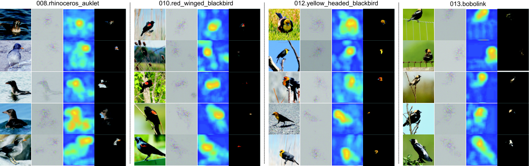
To better understand our model, we adopt three different approaches to visualizing the model response for specific input images. In the first method, we feed an input image to the trained model, and compute responses from the bilinear classifier layer. Based on the ground-truth class label, we create a modified response by zeroing out the part corresponding to negative Frobenius score () for the ground-truth class, and the part to the positive Frobenius scores () in the remaining classifiers, respectively. This is similar to approaches used for visualizing HOG templates by separating the positive and negative components of the weight vector. To visualize the result, we treat as the target and backpropagate the difference to the input image space, similar to [28]. For the second visualization, we compute the magnitude of feature activations averaged across feature channels used by the bilinear classifier. Finally, we produce a third visualization by repeatedly remove superpixels from the input image, selecting the one that introduces minimum drop in classification score This is similar to [26, 39]. In Figure 8, we show some randomly selected images from four different classes in CUB-200-2011 dataset and their corresponding visualizations.
The visualizations all suggest that the model is capable of ignoring cluttered backgrounds and focuses primarily on the bird and even on specific discriminative parts of each bird. Moreover, the highlighted activation region changes w.r.t the bird size and context, as shown in the first panel of Figure 8. For the species “010.red_winged_blackbird”, “012.yellow_headed_blackbird” and “013.bobolink”, the most distinctive parts, intuitively, are the red wings, yellow head and neck, and yellow nape, respectively. Our model naturally appears to respond to and localize these parts. This provides a partial explanation as to why simple global pooling achieves such good results without an explicit spatial transformer or cross-channel pooling architecture (e.g. [21])
6 Conclusion
We have presented an approach for training a very compact low-rank classification model that is able to leverage bilinear feature pooling for fine-grained classification while avoiding the explicit computation of high-dimensional bilinear pooled features. Our Frobenius norm based classifier allows for fast evaluation at test time and makes it easy to impose hard, low-rank constraints during training, reducing the degrees of freedom in the parameters to be learned and yielding an extremely compact feature set. The addition of a co-decomposition step projects features into a shared subspace and yields a further reduction in computation and parameter storage. Our final model can be initialized with a simple PCA step followed by end-to-end fine tuning.
Our final classifier model is one to two orders of magnitude smaller than existing approaches and achieves state-of-the-art performance on several public datasets for fine-grained classification by using only the category label (without any keypoint or part annotations). We expect these results will form a basis for future experiments such as training on weakly supervised web-scale datasets [17], pooling multiple feature modalities and further compression of models for use on mobile devices.
Acknowledgement
This project is supported by NSF grants IIS-1618806, IIS-1253538, DBI-1262547 and a hardware donation from NVIDIA.
References
- [1] R. K. Ando and T. Zhang. A framework for learning predictive structures from multiple tasks and unlabeled data. Journal of Machine Learning Research, 6(Nov):1817–1853, 2005.
- [2] J. Carreira, R. Caseiro, J. Batista, and C. Sminchisescu. Semantic segmentation with second-order pooling. In Computer Vision–ECCV 2012, pages 430–443. Springer, 2012.
- [3] A. Choromanska, M. Henaff, M. Mathieu, G. B. Arous, and Y. LeCun. The loss surfaces of multilayer networks. In AISTATS, 2015.
- [4] M. Cimpoi, S. Maji, I. Kokkinos, S. Mohamed, and A. Vedaldi. Describing textures in the wild. In Proceedings of the IEEE Conference on Computer Vision and Pattern Recognition, pages 3606–3613, 2014.
- [5] M. Cimpoi, S. Maji, and A. Vedaldi. Deep filter banks for texture recognition and segmentation. In Proceedings of the IEEE Conference on Computer Vision and Pattern Recognition, pages 3828–3836, 2015.
- [6] Y. Cui, F. Zhou, Y. Lin, and S. Belongie. Fine-grained categorization and dataset bootstrapping using deep metric learning with humans in the loop. arXiv preprint arXiv:1512.05227, 2015.
- [7] Y. N. Dauphin, R. Pascanu, C. Gulcehre, K. Cho, S. Ganguli, and Y. Bengio. Identifying and attacking the saddle point problem in high-dimensional non-convex optimization. In Advances in neural information processing systems, pages 2933–2941, 2014.
- [8] Y. Gao, O. Beijbom, N. Zhang, and T. Darrell. Compact bilinear pooling. CVPR, 2016.
- [9] S. Huang, Z. Xu, D. Tao, and Y. Zhang. Part-stacked cnn for fine-grained visual categorization. arXiv preprint arXiv:1512.08086, 2015.
- [10] M. Jaderberg, K. Simonyan, A. Zisserman, et al. Spatial transformer networks. In Advances in Neural Information Processing Systems, pages 2008–2016, 2015.
- [11] H. Jégou, M. Douze, and C. Schmid. On the burstiness of visual elements. In Computer Vision and Pattern Recognition, 2009. CVPR 2009. IEEE Conference on, pages 1169–1176. IEEE, 2009.
- [12] P. Kar and H. Karnick. Random feature maps for dot product kernels. In AISTATS, volume 22, pages 583–591, 2012.
- [13] T. Kobayashi. Low-rank bilinear classification: Efficient convex optimization and extensions. International Journal of Computer Vision, 110(3):308–327, 2014.
- [14] S. Kong, S. Punyasena, and C. Fowlkes. Spatially aware dictionary learning and coding for fossil pollen identification. arXiv preprint arXiv:1605.00775, 2016.
- [15] P. Koniusz and A. Cherian. Sparse coding for third-order super-symmetric tensor descriptors with application to texture recognition. CVPR, 2016.
- [16] J. Krause, H. Jin, J. Yang, and L. Fei-Fei. Fine-grained recognition without part annotations. In Proceedings of the IEEE Conference on Computer Vision and Pattern Recognition, pages 5546–5555, 2015.
- [17] J. Krause, B. Sapp, A. Howard, H. Zhou, A. Toshev, T. Duerig, J. Philbin, and L. Fei-Fei. The unreasonable effectiveness of noisy data for fine-grained recognition. arXiv preprint arXiv:1511.06789, 2015.
- [18] J. Krause, M. Stark, J. Deng, and L. Fei-Fei. 3d object representations for fine-grained categorization. In Proceedings of the IEEE International Conference on Computer Vision Workshops, pages 554–561, 2013.
- [19] D. D. Lee and H. S. Seung. Learning the parts of objects by non-negative matrix factorization. Nature, 401(6755):788–791, 1999.
- [20] T.-Y. Lin, A. RoyChowdhury, and S. Maji. Bilinear cnn models for fine-grained visual recognition. In Proceedings of the IEEE International Conference on Computer Vision, pages 1449–1457, 2015.
- [21] L. Liu, C. Shen, and A. van den Hengel. The treasure beneath convolutional layers: Cross-convolutional-layer pooling for image classification. In Proceedings of the IEEE Conference on Computer Vision and Pattern Recognition, pages 4749–4757, 2015.
- [22] S. Maji, E. Rahtu, J. Kannala, M. Blaschko, and A. Vedaldi. Fine-grained visual classification of aircraft. arXiv preprint arXiv:1306.5151, 2013.
- [23] F. Perronnin, J. Sánchez, and T. Mensink. Improving the fisher kernel for large-scale image classification. In European conference on computer vision, pages 143–156. Springer, 2010.
- [24] N. Pham and R. Pagh. Fast and scalable polynomial kernels via explicit feature maps. In Proceedings of the 19th ACM SIGKDD international conference on Knowledge discovery and data mining, pages 239–247. ACM, 2013.
- [25] H. Pirsiavash, D. Ramanan, and C. C. Fowlkes. Bilinear classifiers for visual recognition. In Advances in neural information processing systems, pages 1482–1490, 2009.
- [26] M. T. Ribeiro, S. Singh, and C. Guestrin. ”why should i trust you?”: Explaining the predictions of any classifier. In KDD, 2016.
- [27] M. Simon, E. Rodner, and J. Denzler. Part detector discovery in deep convolutional neural networks. In Computer Vision–ACCV 2014, pages 162–177. Springer, 2014.
- [28] K. Simonyan, A. Vedaldi, and A. Zisserman. Deep inside convolutional networks: Visualising image classification models and saliency maps. arXiv preprint arXiv:1312.6034, 2013.
- [29] K. Simonyan and A. Zisserman. Very deep convolutional networks for large-scale image recognition. arXiv preprint arXiv:1409.1556, 2014.
- [30] J. B. Tenenbaum and W. T. Freeman. Separating style and content with bilinear models. Neural computation, 12(6):1247–1283, 2000.
- [31] A. Vedaldi and K. Lenc. Matconvnet: Convolutional neural networks for matlab. In Proceedings of the 23rd ACM international conference on Multimedia, pages 689–692. ACM, 2015.
- [32] C. Wah, S. Branson, P. Welinder, P. Perona, and S. Belongie. The caltech-ucsd birds-200-2011 dataset. 2011.
- [33] Y. Wang, J. Choi, V. I. Morariu, and L. S. Davis. Mining discriminative triplets of patches for fine-grained classification. CVPR, 2016.
- [34] L. Wolf, H. Jhuang, and T. Hazan. Modeling appearances with low-rank svm. In 2007 IEEE Conference on Computer Vision and Pattern Recognition, pages 1–6. IEEE, 2007.
- [35] M. D. Zeiler and R. Fergus. Visualizing and understanding convolutional networks. In Computer vision–ECCV 2014, pages 818–833. Springer, 2014.
- [36] H. Zhang, T. Xu, M. Elhoseiny, X. Huang, S. Zhang, A. Elgammal, and D. Metaxas. Spda-cnn: Unifying semantic part detection and abstraction for fine-grained recognition. In CVPR, 2016.
- [37] N. Zhang, J. Donahue, R. Girshick, and T. Darrell. Part-based r-cnns for fine-grained category detection. In European Conference on Computer Vision, pages 834–849. Springer, 2014.
- [38] N. Zhang, E. Shelhamer, Y. Gao, and T. Darrell. Fine-grained pose prediction, normalization, and recognition. In ICLR workshop, 2016.
- [39] B. Zhou, A. Lapedriza, J. Xiao, A. Torralba, and A. Oliva. Learning deep features for scene recognition using places database. In Advances in neural information processing systems, pages 487–495, 2014.