When no risk of ambiguity arises, we here employ the standard abbreviated notation of statistical inference (Casella and Berger, 2002), denoting random variables with letters in upper case, and their values, with the same letters but in lower case. Accordingly, the symbols $P(x|y)$ and $P(x)$ always denote the conditional and unconditional probabilities, respectively, of the random variable $X$ taking the value $x$ given that the random variable $Y$ takes the value $y$. Although this notation is common in neuroscience (Nirenberg and Latham, 2003; Quiroga and Panzeri, 2009; Latham and Roudi, 2013), we have found that it may potentially lead to confusing the encoding and the decoding problems. In those cases, we employ the more general symbols $P(X{=}v|Y{=}w)$ and $P(X{=}v)$ to denote the conditional and unconditional probabilities, respectively, that the random variable $X$ takes the value $v$ given that the random variable $Y$ takes the value $w$.

The process of converting stimuli $S$ into neural responses $\mathbf{R}$ (e.g., spike-trains, local-field potentials, electroencephalographic or other brain signals, etc.) is called encoding (Schneidman et al., 2003; Panzeri et al., 2010). The information that $\mathbf{R}$ contains about $S$ is here quantified as

The process of transforming $\mathbf{R}$ into estimated stimuli $\hat{S}$ (or into perceptions, decisions and actions) is called decoding (Schneidman et al., 2003; Panzeri et al., 2010). Under the Bayesian coding hypothesis (Knill and Pouget, 2004; van Bergen et al., 2015), decoding is usually performed using optimal decoders (also called Bayesian or maximum-a-posteriori decoders, and ideal homunculus or observers, among other names; see Eyherabide (2016) and references therein). In their most general form, these decoders map $\mathbf{R}$ into $\hat{S}$ according to the following formula

The joint probability $P(s,\hat{s})$ of the presented and estimated stimuli, also called confusion matrix (Quiroga and Panzeri, 2009), can be computed as follows

Any representation of the recorded neural activity into a vector $\mathbf{R}{=}[R_{1},\ldots,R_{N}]$ of $N$ response aspects is usually called a neural code. The aspects may represent, for example, neurons, neural populations, or cortical areas (Nirenberg and Latham, 2003; Schneidman et al., 2003; Latham and Nirenberg, 2005; Eyherabide and Samengo, 2013; Eyherabide, 2016), but also first-spike latencies, spike counts, and spike-timing variability (Furukawa and Middlebrooks, 2002; Nelken and Chechik, 2007; Eyherabide and Samengo, 2010b; Eyherabide, 2016). To assess what aspects are informative, $\mathbf{R}$ is usually transformed into another neural code $\mathbf{\hat{R}}$, often called reduced code (Schneidman et al., 2003; Eyherabide and Samengo, 2010b), through stimulus-independent deterministic functions that typically preserve a limited number of response aspects or a coarser version of the existing ones. As we note here, this assessment can also be conducted using stimulus-independent stochastic functions, here called stochastic codes (see Results). In both cases, the data processing theorem ensures that $I_{\mathbf{R}}{\geq}I_{\mathbf{\hat{R}}}$.

Given a neural code $\mathbf{R}{=}[R_{1},\ldots,R_{N}]$, the aspects are said noise independent if $P(\mathbf{r}|s){=}P^{{N\hskip-1.22911ptI\hskip-1.22911pt}\hskip-0.40974pt}(\mathbf{r}|s)$ for all $\mathbf{r}$ and $s$, with $P^{{N\hskip-1.22911ptI\hskip-1.22911pt}\hskip-0.40974pt}(\mathbf{r}|s){=}\prod_{n=1}^{N}{P(r_{n}|s)}$. Otherwise, they are said noise correlated. As mentioned in Eyherabide (2016), this definition should not be confused with both those that average over stimuli (Gawne and Richmond, 1993; Pereda et al., 2005; Womelsdorf et al., 2012), and therefore prone to cancellation effects and to confusing noise correlations with activity correlations (Nirenberg and Latham, 2003; Schneidman et al., 2003; Eyherabide, 2016); and those that are limited to specific linear or nonlinear types of correlations (Pereda et al., 2005; Cohen and Kohn, 2011; Latham and Roudi, 2013).

From an information-theoretical standpoint, the importance of response aspects in neural encoding has previously been quantified in many ways (see Eyherabide and Samengo, 2010b, and references therein), out of which we chose the following four measures

In this study, stochastic functions always exist that transform $\mathbf{R}$ into $\mathbf{\hat{R}}$ in a stimulus-independent manner, unless otherwise stated. Hence, the transformation from $\mathbf{R}$ into $\hat{S}$ can be interpreted as a sequential process (Geisler, 1989; Eyherabide and Samengo, 2013) in which $\mathbf{R}$ is first transformed into $\mathbf{\hat{R}}$, then into $\mathbf{\hat{S}}$, and finally into $\hat{S}$. Consequently, $\Delta I_{\mathbf{\hat{R}}}$, $\Delta I_{\mathbf{\hat{S}}}$ and $\Delta I_{\hat{S}}$ can be interpreted as accumulated information losses after the first, second and third transformations, respectively, whereas $\Delta A_{\mathbf{\hat{R}}}$, as the accuracy loss after the first transformation. The data processing theorems ensure that all the above measures are never negative.

The above four measures are here regarded as encoding-oriented, even though the last three use optimal decoders. Indeed, our classification does not follow previous criteria based on the nature of the measure (Schneidman et al., 2003; Quiroga and Panzeri, 2009), which are often obscure and arguably questionable (Eyherabide, 2016). Specifically, consider $\Delta I_{\mathbf{\hat{R}}}$ and $\Delta I_{\hat{S}}$. The former has always been regarded as an encoding measure even when no stimulus-independent function from $\mathbf{R}$ into $\mathbf{\hat{R}}$ exists (Nirenberg and Latham, 2003), and even though it need not be conclusive about the actual encoding mechanism (see Results). Classifying the latter as an encoding measure may seem questionable because it is based on encoded information, but in the output of a decoder (Quiroga and Panzeri, 2009; Eyherabide, 2016). However, in the light of previous studies on the role of noise correlations in neural decoding (Nirenberg et al., 2001; Nirenberg and Latham, 2003; Latham and Nirenberg, 2005; Eyherabide, 2016), classifying it as a decoding measure may also seem questionable because the decoder is trained and tested with the same responses.

Notice that Eq (5) has previously been used to quantify the importance of noise correlations in encoding information (Schneidman et al., 2003; Eyherabide et al., 2009). In those cases, $\mathbf{\hat{R}}$ has been replaced with surrogate responses generated assuming that neurons are noise independent, here denoted $\mathbf{R}^{N\hskip-1.22911ptI}$. However, we can prove the following theorem:

Consequently, $\Delta I_{\mathbf{R}^{N\hskip-1.10413ptI}}$, $\Delta A_{\mathbf{R}^{N\hskip-1.10413ptI}}$, $\Delta I_{\mathbf{S}^{N\hskip-1.10413ptI}}$, and $\Delta I_{S^{N\hskip-1.10413ptI}}$ (with $\mathbf{S}^{N\hskip-1.22911ptI}$ and $S^{N\hskip-1.22911ptI}$ analogous to $\mathbf{\hat{S}}$ and $\hat{S}$, respectively, but for optimal decoders operating on $\mathbf{R}^{N\hskip-1.22911ptI}$) can be ensured neither to be nonnegative nor to compare information of the same type (Nirenberg and Latham, 2003), unless a stochastic code exists that maps $\mathbf{R}$ into $\mathbf{R}^{N\hskip-1.22911ptI}$.

From and information-theoretical standpoint, the importance of response aspects in neural decoding has been previously quantified in many ways (see Eyherabide and Samengo, 2013, and references therein), out of which we chose the following five that are more closely related to optimal decoding

In addition, we can generalize the flaws of previous definitions of $P(s|\mathbf{\hat{r}},\theta)$ found in Eyherabide and Samengo (2013) as follows

Consequently, here we define $P(s|\mathbf{\hat{r}},\theta)$ as follows

In addition, we will compute the accuracy loss from the decoding perspective as follows

The measures $\Delta I^{D\hskip-1.22911pt}$, $\Delta I^{D\hskip-1.22911ptL\hskip-1.22911pt}$, $\Delta I^{L\hskip-1.22911ptS\hskip-1.22911pt}$ and $\Delta I^{B\hskip-1.22911pt}$ have all been previously regarded as quantifying the information loss caused when optimal decoders operate on $\mathbf{R}$, but make decisions assuming that the input is $\mathbf{\hat{R}}$. The first measure, $\Delta I^{D\hskip-1.22911pt}$, was introduced by Nirenberg et al. (2001) with $P(S{=}s|\mathbf{\hat{R}}{=}\mathbf{r}){=}P^{{N\hskip-1.22911ptI\hskip-1.22911pt}\hskip-0.40974pt}(s|\mathbf{r})$, and later extended to any $P(S{=}s|\mathbf{\hat{R}}{=}\mathbf{r})$ (Nirenberg and Latham, 2003; Quiroga and Panzeri, 2009; Latham and Roudi, 2013; Eyherabide, 2016). Although often overlooked (Quiroga and Panzeri, 2009; Latham and Roudi, 2013), $\Delta I^{D\hskip-1.22911pt}$ presents the following two difficulties: first, it can exceed $I_{\mathbf{R}}$ and tend to infinity if $P(s|\mathbf{\hat{r}}){=}0$ when $P(s|\mathbf{r}){>}0$ for some $s$ and $\mathbf{r}{=}\mathbf{\hat{r}}$ (Schneidman et al., 2003); and second, here we note that it may be undefined if $P(\mathbf{\hat{r}}){=}0$ when $P(\mathbf{r}){>}0$ for some $\mathbf{r}{=}\mathbf{\hat{r}}$ (Fig 3B).

The second measure, $\Delta I^{D\hskip-1.22911ptL\hskip-1.22911pt}$, was introduced by Latham and Nirenberg (2005) and has always been deemed exact (Latham and Nirenberg, 2005; Oizumi et al., 2009; Quiroga and Panzeri, 2009; Ince et al., 2010; Oizumi et al., 2010; Latham and Roudi, 2013; Oizumi et al., 2016). Latham and Nirenberg (2005) showed that, unlike $\Delta I^{D\hskip-1.22911pt}$, $\Delta I^{D\hskip-1.22911ptL\hskip-1.22911pt}{\leq}I_{\mathbf{R}}$, but their proof ignored the cases mentioned in our theorems 2 and 3. Nevertheless, these theorems imply that $\Delta I^{D\hskip-1.22911ptL\hskip-1.22911pt}{\leq}I_{\mathbf{R}}$ through Eq (10). However, Eyherabide and Samengo (2013) has shown that $\Delta I^{D\hskip-1.22911ptL\hskip-1.22911pt}$ may exceed both $\Delta I^{L\hskip-1.22911ptS\hskip-1.22911pt}$ and $\Delta I^{B\hskip-1.22911pt}$; and Eyherabide (2016), that it may overestimate the loss when decoding together neural populations that transmit independent information.

The third measure, $\Delta I^{L\hskip-1.22911ptS\hskip-1.22911pt}$, was introduced by Ince et al. (2010) and quantifies the difference between two encoded informations: the one in $\mathbf{R}$, and the one in the output of decoders that, after observing $\mathbf{r}$, produce a stimulus list sorted according to $P(S{=}s|\mathbf{\hat{R}}{=}\mathbf{r})$. The fourth measure, $\Delta I^{B\hskip-1.22911pt}$, quantifies the difference between the information encoded in $\mathbf{R}$ and that encoded in the output of an optimal decoder constructed using $P(s|\mathbf{\hat{r}})$. When the number of stimuli is two, $\Delta I^{L\hskip-1.22911ptS\hskip-1.22911pt}$ reduces to $\Delta I^{B\hskip-1.22911pt}$ (Eyherabide and Samengo, 2013; Eyherabide, 2016).

As we show in Fig 3B, $\Delta I^{D\hskip-1.22911pt}$, $\Delta I^{L\hskip-1.22911ptS\hskip-1.22911pt}$, $\Delta I^{B\hskip-1.22911pt}$, and $\Delta A^{B\hskip-1.22911pt}$ are undefined if the actual responses $\mathbf{R}$ are not contained within the surrogate responses $\mathbf{\hat{R}}$. The result for $\Delta I^{D\hskip-1.22911pt}$ was already explained in the first paragraph. For the other measures, our observation stems from the fact that, for the missing responses, an optimal decoder simply does not know what output should be produced. Our observation does not apply to $\Delta I^{D\hskip-1.22911ptL\hskip-1.22911pt}$ due to our theorems 2 and 3, but can be easily seen from the definition of $\Delta I^{D\hskip-1.22911ptL\hskip-1.22911pt}$ as a communication information loss (Latham and Nirenberg, 2005; Oizumi et al., 2010; Eyherabide, 2016). Indeed, the fact that optimal decoders may fail to operate on $\mathbf{R}$ due to the missing responses in $\mathbf{\hat{R}}$ indicates that no information can be reliably transmitted, thereby yielding $\Delta I^{D\hskip-1.22911ptL\hskip-1.22911pt}{=}I_{\mathbf{R}}$ (Latham and Nirenberg, 2005; Eyherabide, 2016).

Finally, notice that decoding measures may yield different and sometimes contradictory results (Oizumi et al., 2009; Oizumi et al., 2010; Eyherabide and Samengo, 2013; Latham and Roudi, 2013). However, the contradictions can be partially resolved by noticing that they have been previously derived using different notions of information. The reader is referred to Eyherabide (2016) and references therein for further remarks on these measures and notions.

The role of first-spike latencies, spike counts, or other response aspects in encoding information — the encoding problem — and in brain computations — the decoding problem — has previously been assessed, for example, using methods based either on information theory or on decoders (Quiroga and Panzeri, 2009). For decades, methods based on information theory have often been related to the encoding problem, whereas methods based on decoders have often been related to the decoding problem. However, here we argue that the nature of the employed method is not reliably related to its operational significance, at least from the observer perspective.

Information-based methods typically compare the information encoded in two representations of the neural response, usually called neural codes and here denoted $\mathbf{R}$ and $\mathbf{\hat{R}}$. The code $\mathbf{R}$ typically preserves all response aspects, whereas the code $\mathbf{\hat{R}}$ usually arises from some transformation of $\mathbf{R}$ that ignores some response aspects, or at least the additional information they carry. The ignored response aspects are usually deemed inessential for encoding information when the information in $\mathbf{R}$ and $\mathbf{\hat{R}}$ is approximately equal, and important otherwise. However, the encoded information need not provide conclusive insight about the encoding mechanisms, but about the read out mechanisms.

To illustrate this, consider the hypothetical experiment shown in Fig 1A. There, the responses of a single neuron elicited by two visual stimuli have been characterized by counting the number of spikes within consecutive time-bins starting from the stimulus onset. This characterization preserves all the encoded information regardless of whether the bin size is $5$, $10$, or $15\,ms$, thereby shedding limited insight into the actual spike-time precision employed by the encoding mechanism, which is $10\,ms$. However, this result certainly proves that such knowledge is inessential for ideal observers, who can read the spike trains without loss using any of the aforementioned bin sizes.

Decoder-based methods usually compare the decoded informations or the decoding accuracies of two decoders: one constructed using $\mathbf{R}$ and another one constructed using $\mathbf{\hat{R}}$. The ignored response aspects are usually deemed inessential for decoding information when the information extracted by these two decoders is approximately equal, and important otherwise. However, the information extracted by optimal decoders trained and tested with surrogate responses $\mathbf{R}^{N\hskip-1.22911ptI}$ generated assuming that neurons are noise independent (Quiroga and Panzeri, 2009) need not provide insight into the necessity for taking into account noise correlations when constructing optimal decoders (Nirenberg and Latham, 2003; Eyherabide, 2016).

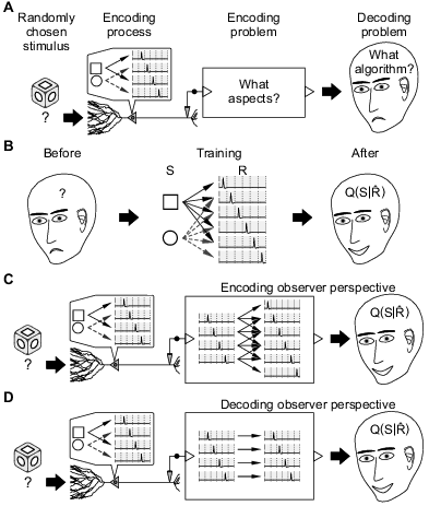
Our observations motivate us to reformulate the coding problem from the perspective of an ideal observer or organism (Fig 2A). Within this perspective, we devise the encoding problem as concerning the losses caused when the ideal observers either can only see and are only allowed to see not the actual neural responses ($\mathbf{R}$), but a transformed version of them ($\mathbf{\hat{R}}$) that preserves a limited number of response aspects (Fig 2C). The decoding problem is here interpreted analogously to the decoding perspective of the role of noise correlations, namely, as concerning the losses caused when observers make decisions assuming that they see $\mathbf{\hat{R}}$ instead of $\mathbf{R}$ (Fig 2D). Mathematically, both problems can be tackled by training ideal observers not with $\mathbf{R}$ but with $\mathbf{\hat{R}}$ (Fig 2B). However, within the encoding problem, the ideal observer operates on $\mathbf{\hat{R}}$, whereas within the decoding problem, the ideal observer operates on $\mathbf{R}$.

These conceptual and operational differences notwithstanding, decoding-oriented measures of loss have previously been regarded as generalizing their encoding-oriented counterparts (Nirenberg et al., 2001; Nirenberg and Latham, 2003; Quiroga and Panzeri, 2009; Latham and Roudi, 2013). Unfortunately, these claims ought to be observed with caution for at least three reasons: they need not be accurate, potentially confuse encoding and decoding, and are limited to specific types of codes. In this section, we will explain and justify these reasons.

Concerning the accuracy of the claims, Nirenberg and Latham (2003) claimed that their version $\Delta I^{D\hskip-1.22911pt}$ for studying noise correlations is always positive and reduces to the difference in encoded information between two neural codes: one using large time-bins and another one using small time-bins. However, this difference can be positive or negative, regardless of the order in which the informations are subtracted, thereby contradicting the putative positivity of both $\Delta I^{D\hskip-1.22911pt}$ and the measure they proposed. Indeed, in Fig 1B, using time-bins of $5$ or $15\,ms$ preserves all the encoded information, but using intermediate time-bins of $10\,ms$ preserves none, thereby proving our statement.

Our finding seemingly contradicts previous experimental studies (Reinagel and Reid, 2000; Quiroga and Panzeri, 2013) and, most importantly, the data processing theorem (Cover and Thomas, 2006). Indeed, it shows that previous experimental findings of encoded information monotonically decreasing with bin size are not completely attributable to time discretization. However, it does not violate the data processing theorem because the code with $15\,ms$ time-bins cannot be derived from that with $10\,ms$ time-bins through stimulus-independent transformations.

Actually, the study of Nirenberg and Latham (2003) proposed a generalization of $\Delta I^{D\hskip-1.22911pt}$, as opposed to a reduction of it, but unfortunately it cannot be interpreted in the same way. Indeed, their generalization compares the additional costs of using two different codes for constructing two decoders, respectively, that are then employed to decode a third code. Thus, this generalization need not be suitable for addressing the decoding problem, which concerns the losses caused by decoding a code assuming that it is another one, unless it is first reduced to $\Delta I^{D\hskip-1.22911pt}$.

The confusion between encoding and decoding arises from the particular choice of probabilities that previous studies (Nirenberg and Latham, 2003; Quiroga and Panzeri, 2009; Latham and Roudi, 2013) have employed when computing $\Delta I^{D\hskip-1.22911pt}$ for stimulus-independent transformations of the original codes representing the neural responses, but we defer the proofs until the last section of Results. Most importantly, the above generalization and computations of $\Delta I^{D\hskip-1.22911pt}$, as conducted in previous studies (Nirenberg and Latham, 2003; Quiroga and Panzeri, 2009; Latham and Roudi, 2013), together with their criticism (Schneidman et al., 2003), are actually limited to stimulus-independent deterministic transformations, often called reduced codes, as opposed stochastic ones, here called stochastic codes. In the next section we characterize this codes, and in the one immediately after, we will assess what role they play in encoding and decoding from the observer perspective.

Stochastic codes arise naturally when studying the importance of specific response aspects (Eyherabide and Samengo, 2010b). However, stochastic codes are most valuable when studying other response aspects such as spike-time precision (Kayser et al., 2010; Quiroga and Panzeri, 2009), response discrimination (Victor and Purpura, 1996; Victor, 2005; Rusu and Florian, 2014), noise along neural pathways (Nelken, 2008), and even noise correlations. In these cases, the use of reduced codes may be questionable, if not impossible. In this section, we will first illustrate these claims before giving a formal definition of stochastic codes.

Consider the hypothetical experiment in Fig 3A, in which the neural responses $\mathbf{R}{=}[L,C]$ can be completely characterized by the first-spike latencies ($L$) and the spike counts ($C$). The importance of $C$ can be studied not only using a reduced code that replaces all its values with a constant (Fig 3B), but also a stochastic code that shuffles the values of $C$ across all responses with the same $L$ (Fig 3C), or even a stochastic code that preserves the original value of $L$ but chooses the value of $C$ from some possibly $L-$dependent arbitrary probability distribution (Fig 3D).

Using either reduced or stochastic codes in the previous example seemingly yields the same result (but see next section). However, this need not always be the case. For example, spike-time precision has previously been studied using at least three different methods, here called binning, bin-shuffling and jittering. Binning is perhaps the most common of the three methods and consists in transforming the recorded spike trains into discrete-time sequences (Fig 1), thereby yielding a reduced code that can be interpreted as a stochastic code (Fig 3). Bin-shuffling consists in randomly permuting spikes and silences within consecutive non-overlapping windows (Fig 4A), which inherently constitutes a stochastic code.

These two methods are equivalent in the sense that the responses generated by each method can be related through stimulus-independent stochastic functions to those generated by the other, and therefore contain the same amount and type of information. However, both methods suffer from the same drawback: they both treat spikes differently depending on their location within the time window. Indeed, both methods preserve the distinction between two spikes located at different time bins, but not within the same time bin, even if the separation between the spikes is the same.

The third method, jittering, consists in shuffling the recorded spikes within time windows centered at each spike (Fig 4B). Notice that the responses generated by this method need not be related to the responses generated by the other two methods through stimulus-independent stochastic functions, nor vice versa. However, this method inherently yields a stochastic code, and, unlike the previous methods, treats all spikes in the same manner.

As another example, consider the effect of response discrimination, as studied in the seminal work of Victor and Purpura (1996). There, two responses were considered indistinguishable when some measure of distance between the responses was less than some predefined value. However, the distances were there used for transforming neural responses through a method based on cross-validation that, as we note here, is not guaranteed to be stimulus-independent as stochastic codes. Other methods exist which simply merge indistinguishable responses thereby yielding a reduced code, but these methods are limited to distances that are transitive.

Here we overcome these limitations by devising a method based on stochastic codes, which mimics the operation of an observer that confuses responses by randomly treating them as if it was another response. This method includes those based on reduced codes, and even those based on possibly non-symmetrical and non-metric measures of response similarity. Unlike the previous methods, this one can effectively be applied to the example shown in Fig 4C.

Formally, Stochastic codes are here defined as neural codes $\mathbf{\hat{R}}$ that can be obtained through stimulus-independent stochastic functions of other codes $\mathbf{R}$. After observing that $\mathbf{R}$ adopted the value $\mathbf{r}$, these functions produce a single value $\mathbf{\hat{r}}$ for $\mathbf{\hat{R}}$ chosen with transition probabilities $Q(\mathbf{\hat{r}}|\mathbf{r})$ such that

The problem of finding a feasible $Q(\mathbf{\hat{r}}|\mathbf{r})$ can be readily solved using linear programming (Boyd and Vandenberghe, 2004), which we can simplify by noticing the following two properties

• 1)

  $Q(\mathbf{\hat{r}}|\mathbf{r}){=}0$ if $P(s,\mathbf{r}){>}0$ and $P(s,\mathbf{\hat{r}}){=}0$, for otherwise it would contradict the definition of stochastic codes; and

• 2)

  A feasible $Q(\mathbf{\hat{r}}|\mathbf{r})$ never exists if $I_{\mathbf{\hat{R}}}{>}I_{\mathbf{R}}$, for otherwise it would contradict the data processing theorem.

However, notice that stochastic codes need not always exist. For example, in Fig 4E, the condition $I_{\mathbf{R}}{<}I_{\mathbf{R}^{N\hskip-1.10413ptI}}$ always hold, and therefore no stochastic code can map $\mathbf{R}$ into $\mathbf{R}^{N\hskip-1.22911ptI}$. Notice that Schneidman et al. (2003) employed an analogous example, but involving different neurons instead of response aspects, only for comparing $\Delta I^{D\hskip-1.22911pt}$ with $\Delta I_{\mathbf{\hat{R}}}$, and ignoring whether $\mathbf{R}^{N\hskip-1.22911ptI}$ constitutes as a stochastic code. Finally, stochastic codes must not be confused with probabilistic population codes (Knill and Pouget, 2004), stimulus-dependent noise, decoding algorithms based on cross-validation (Victor and Purpura, 1996; Quiroga and Panzeri, 2009), and list decoding (Schneidman et al., 2003; Ince et al., 2010; Eyherabide and Samengo, 2013).

Like reduced codes, stochastic codes are here defined as stimulus-independent transformations of another code. Accordingly, both types of codes preserve only information contained in the original code that limits the decoded information when decoders operate on them. Although stochastic codes may include more responses than the original codes, this should arguably raise no concerns (Nirenberg and Latham, 2003; Schneidman et al., 2003) because the transformations that define them are stimulus independent and can be implemented during decoding. Thus, for stochastic codes, the encoding and the decoding problems may be related as they are for reduced codes, even when arising from ignoring noise correlations (Fig 4D).

We tested this hypothesis by comparing three encoding-oriented measures of information loss ($\Delta I_{\mathbf{\hat{R}}}$, $\Delta I_{\mathbf{\hat{S}}}$, $\Delta I_{\hat{S}}$) and one of accuracy loss ($\Delta A_{\mathbf{\hat{R}}}$), with four decoding-oriented measures of information loss ($\Delta I^{D\hskip-1.22911pt}$, $\Delta I^{D\hskip-1.22911ptL\hskip-1.22911pt}$, $\Delta I^{L\hskip-1.22911ptS\hskip-1.22911pt}$, $\Delta I^{B\hskip-1.22911pt}$) and one of accuracy loss ($\Delta A^{B\hskip-1.22911pt}$). Their definitions, rationale, and classification are given in Methods. We found that, for the stochastic codes in Figures 3–5, the encoding-oriented measures were greater or less than the decoding-oriented measures depending on the case and the probabilities (Table 1). Consequently, our results refute the above hypothesis and, most importantly, prove that previous controversies about encoding and decoding transcend the study of noise correlations.

Our conclusions may seem puzzling because the data processing theorems ensure that neither $\Delta I_{\mathbf{\hat{R}}}$ can exceed the information loss, nor $\Delta A_{\mathbf{\hat{R}}}$ the accuracy loss, caused when decoders operate on $\mathbf{\hat{R}}$. However, the data processing theorems are not violated because encoding-oriented measures are related to decoders that operate on $\mathbf{\hat{R}}$, whereas decoding-oriented measures are related to decoders that operate directly on $\mathbf{R}$ (Fig 2D).

To gain additional insight, we divided the stochastic codes in four groups. In the first group (Fig 4D), noise correlations can be ignored through stochastic codes, but the results remain unchanged. Consequently, contrary to previously thought (Nirenberg and Latham, 2003), the discrepancy between encoding- and decoding-oriented measures cannot be completely attributed to surrogate responses generated through stimulus-dependent transformations, or containing responses with information not present in the original neural responses. However, we can prove the following theorem

We tested if the discrepancy between encoding- and decoding-oriented measures stems from the aforementioned dependencies by comparing the values they attain within the second group of stochastic codes (Fig 4 B,C). For these codes, which arise naturally when studying spike-time precision or response discrimination, we found that the dependencies never occur (namely, $Q(\mathbf{\hat{R}}|\mathbf{R})$ is independent on $P(S,\mathbf{R})$) but the results remain unchanged. Therefore, we conclude that the aforementioned discrepancy cannot be attributed to these dependencies, and can arise not only when studying noise correlations, but when studying other response aspects even if defined through constant and stimulus-response-independent transformations.

Further inspection shows that the discrepancy occurs even when stochastic codes only contain responses present in the original codes (Fig 4C), and both in the amount and in the type of information (Fig 5B). To prove the latter, consider that an ideal observer is trained using the noisy data $\mathbf{\hat{R}}$ shown in Fig 7A, but it is asked to operate on the quality data $\mathbf{R}$ shown in Fig 7B. The information losses $\Delta I_{\mathbf{\hat{R}}}$, $\Delta I^{D\hskip-1.22911pt}$, and $\Delta I^{D\hskip-1.22911ptL\hskip-1.22911pt}$ produced by this ideal observer are all equal to $I_{\mathbf{R}}/2$ regardless of whether $\mathbf{R}$ is transformed into $\mathbf{\hat{R}}$ before showing them to the ideal observer (the encoding problem) or not (the decoding problem).

However, the aforementioned transformation causes some responses to occur for all stimuli, thereby preserving only some information about frames ($I(S_{F},\mathbf{\hat{R}}){=}I(S_{F},\mathbf{R})/3$) and letters ($I(S_{L},\mathbf{\hat{R}}){=}2\,I(S_{L},\mathbf{R})/3$). In other words, within the encoding problem, $\mathbf{\hat{R}}$ causes a partial information loss $\Delta I_{\mathbf{\hat{R}}}$ that is composed of both frame and letter information. On the contrary, within the decoding problem, $\mathbf{\hat{R}}$ causes no information loss about letters but a total information loss about frames. We can prove the former by noticing that, for the responses that actually occur in $\mathbf{R}$, the ideal observer trained with $\mathbf{\hat{R}}$ can perfectly identify the letters (because $P(\hat{C}{=}2|S_{L}{=}\mathrm{A}){=}P(\hat{C}{=}4|S_{L}{=}\mathrm{B}){=}1$). We can prove the latter by noticing that $P(\hat{l}|\hbox to8.7pt{\vbox to8.03pt{\pgfpicture\makeatletter\hbox{\hskip 4.34999pt\lower-4.01665pt\hbox to0.0pt{\lxSVG@begingroup@{_scopebegin=1} \lxSVG@begingroup@{stroke=#000000} \lxSVG@begingroup@{fill=#000000} \lxSVG@setlinewidth{\the\pgflinewidth}\lxSVG@begingroup@{stroke-width=0.4pt} \lx@inpgf@ignorespaces\nullfont\hbox to0.0pt{\lxSVG@begingroup@{_scopebegin=1} {{}}\lx@inpgf@ignorespaces\hbox{\hbox{{\lxSVG@begingroup@{_scopebegin=1} {{}{}{{ {}{}}}{ {}{}} {{}{{\lx@inpgf@ignorespaces}}}{{}{\lx@inpgf@ignorespaces}}{}{{}{\lx@inpgf@ignorespaces}} {{}\lxSVG@stroke\lxSVG@drawpath@unclipped{M -5.74 -5.28 h 11.48 v 10.56 h -11.48 Z}{fill:none} \lx@inpgf@ignorespaces }{{{{\lx@inpgf@ignorespaces}}\lxSVG@begingroup@{_scopebegin=1} \lxSVG@transformcm{1.0}{0.0}{0.0}{1.0}{-3.75pt}{-3.41666pt}\lxSVG@begingroup@{transform=matrix(1.0 0.0 0.0 1.0 -5.19 -4.73)} \pgfsys@hbox{58}\lxSVG@closescope }}} \lxSVG@closescope }}} \lxSVG@closescope {{ {}{}{}}}{\lx@inpgf@ignorespaces}{\lx@inpgf@ignorespaces}\hss}\lxSVG@discardpath\lxSVG@closescope \hss}}\lxSVG@closescope\endpgfpicture}}){=}P(\hat{l}|\hbox to8.58pt{\vbox to8.58pt{\pgfpicture\makeatletter\hbox{\hskip 4.28789pt\lower-4.28789pt\hbox to0.0pt{\lxSVG@begingroup@{_scopebegin=1} \lxSVG@begingroup@{stroke=#000000} \lxSVG@begingroup@{fill=#000000} \lxSVG@setlinewidth{\the\pgflinewidth}\lxSVG@begingroup@{stroke-width=0.4pt} \lx@inpgf@ignorespaces\nullfont\hbox to0.0pt{\lxSVG@begingroup@{_scopebegin=1} {{}}\lx@inpgf@ignorespaces\hbox{\hbox{{\lxSVG@begingroup@{_scopebegin=1} {{}{{{}}}{{}}{}{}{\lx@inpgf@ignorespaces}{\lx@inpgf@ignorespaces}{}{}{}{}{}{{}\lxSVG@stroke\lxSVG@drawpath@unclipped{M 5.66 0 C 5.66 3.12 3.12 5.66 0 5.66 C -3.12 5.66 -5.66 3.12 -5.66 0 C -5.66 -3.12 -3.12 -5.66 0 -5.66 C 3.12 -5.66 5.66 -3.12 5.66 0 Z M 0 0}{fill:none} \lx@inpgf@ignorespaces }{{{{\lx@inpgf@ignorespaces}}\lxSVG@begingroup@{_scopebegin=1} \lxSVG@transformcm{1.0}{0.0}{0.0}{1.0}{-3.75pt}{-3.41666pt}\lxSVG@begingroup@{transform=matrix(1.0 0.0 0.0 1.0 -5.19 -4.73)} \pgfsys@hbox{58}\lxSVG@closescope }}} \lxSVG@closescope }}} \lxSVG@closescope {{{}}}{\lx@inpgf@ignorespaces}{\lx@inpgf@ignorespaces}\hss}\lxSVG@discardpath\lxSVG@closescope \hss}}\lxSVG@closescope\endpgfpicture}})$ whenever $\hat{l}$ adopts a value that actually occurs in $\mathbf{R}$, namely $2$ or $3$. Analogous computations yield analogous results for the hypothetical experiment shown in Fig 5B.

These results contrast with those found in studies of noise correlations in two ways. First, those studies employed surrogate responses generated through stimulus-dependent transformations and often contain responses with information not present in the original neural responses. Second, for those surrogate responses, we can prove that $\Delta I^{D\hskip-1.22911ptL\hskip-1.22911pt}$ cannot reach $100\,\%$ unless $\Delta I_{\mathbf{\hat{R}}}$ does as well. Specifically, we can prove the following theorem

In the third group (Fig 3D and Fig 4A), $\Delta I_{\mathbf{\hat{R}}}{=}\Delta I^{D\hskip-1.22911pt}{=}\Delta I^{D\hskip-1.22911ptL\hskip-1.22911pt}$, $\Delta I_{\mathbf{\hat{S}}}{=}\Delta I^{L\hskip-1.22911ptS\hskip-1.22911pt}$, $\Delta I_{\hat{S}}{=}\Delta I^{B\hskip-1.22911pt}$, and $\Delta A_{\mathbf{\hat{R}}}{=}\Delta A^{B\hskip-1.22911pt}$. We can prove that these relations arise whenever the mapping from $\mathbf{R}$ into $\mathbf{\hat{R}}$ can be described using positive-diagonal idempotent stochastic matrices (Högnäs and Mukherjea, 2011). Specifically, we can prove the following theorem

This theorem is unnecessary for the quantitative equality between encoding- and decoding-oriented measures, but ensures that the equalities hold not only in amount but also in type. For example, in Fig 5B, we found that $\Delta I_{\mathbf{\hat{R}}}{=}\Delta I_{\mathbf{\hat{S}}}{=}\Delta I_{\hat{S}}{=}\Delta I^{D\hskip-1.22911pt}{=}\Delta I^{D\hskip-1.22911ptL\hskip-1.22911pt}{=}\Delta I^{L\hskip-1.22911ptS\hskip-1.22911pt}{=}\Delta I^{B\hskip-1.22911pt}{=}50\,\%$ and $\Delta A_{\mathbf{\hat{R}}}{=}\Delta A^{B\hskip-1.22911pt}{\approx}67\,\%$ even though theorem 6 does not hold. However, the losses are not necessarily of the same type as we proved before. Most importantly, it formally justifies and clarifies the pervasive idea that, for reduced codes, the decoding-oriented measures reduce to their encoding-oriented counterparts. Indeed, the fourth group shows that, when not fulfilled, decoding-oriented measures can exceed their encoding-oriented counterparts (Fig 5A), or even be undefined (Fig 3B; see Methods). Consequently, contrary to previous studies (Nirenberg and Latham, 2003; Quiroga and Panzeri, 2009; Latham and Roudi, 2013), deterministic transformations need not ensure that the encoding and the decoding problems are related.

These results also reveal unexpected confounds in Nirenberg and Latham (2003); Quiroga and Panzeri (2009); Latham and Roudi (2013) that invalidate their conclusions by turning otherwise decoding-oriented measures into encoding-oriented ones. To reveal and resolve the flaws in the aforementioned studies, recall the experiment in Fig 5A. There, $\mathbf{\hat{R}}{=}f(\mathbf{R})$, with $f$ being a deterministic bijective function. According to the above studies, $\Delta I^{D\hskip-1.22911pt}$ should be computed through Eq (9) but with $P(S{=}s|\mathbf{\hat{R}}{=}\mathbf{r})$ replaced by $Q(s|\mathbf{r}){\propto}P(s)\,P(f(\mathbf{r})|s)$. Because $f$ is bijective, $Q(s|\mathbf{r}){=}P(s|\mathbf{r}){=}P(S{=}s|\mathbf{\hat{R}}{=}f(\mathbf{r}))$. However, we can prove the following theorem

In practice, our results open up the possibility of increasing the efficiency of decoders constructed with approximate descriptions of the neural responses, usually called approximate or mismatched decoders, by adding suitable amounts and types of noise to the decoder input. To see this, recall the example of Fig 7 in which a decoder constructed with noisy data ($\mathbf{\hat{R}}$; Fig 7A) was employed to decode quality data ($\mathbf{R}$; Fig 7B), thereby causing the information losses $\Delta I^{D\hskip-1.22911pt}{=}\Delta I^{D\hskip-1.22911ptL\hskip-1.22911pt}{=}I_{\mathbf{R}}/2$. These losses can be decreased by feeding the decoder with a degraded version $\mathbf{\breve{R}}$ of the quality data (Fig 7D) generated through a stimulus-independent transformation that adds latency noise (Fig 7E). Decoding $\mathbf{R}$ as if it was $\mathbf{\hat{R}}$ by first transforming $\mathbf{R}$ into $\mathbf{\breve{R}}$ results in $\Delta I^{D\hskip-1.22911pt}{=}\Delta I^{D\hskip-1.22911ptL\hskip-1.22911pt}{=}I_{\mathbf{R}}/3$, thereby recovering $33\,\%$ of the information previously lost. On the contrary, adding spike-count noise will tend to increase the losses. Thus, we have proved that adding suitable amounts and type of noise can increase the performance of approximate decoders even for response aspects beyond noise correlations. In addition, this result also indicates that, contrary to previously thought (Shamir, 2014), decoding algorithms need not match the encoding mechanisms for performing optimally from an information-theoretical standpoint.

This work was supported by the Ella and Georg Ehrnrooth Foundation.

In Fig 3 , the transition probabilities $Q(\mathbf{\hat{R}}|\mathbf{R})$ are defined as follows

In Fig 4 , the transition probabilities $Q(\mathbf{\hat{R}}|\mathbf{R})$ are defined using matrices in which row and column indexes enumerate $\mathbf{R}$ and $\mathbf{\hat{R}}$, respectively, according to their latencies in increasing order, thereby yielding

In Fig 5 , the transition probabilities $Q(\mathbf{\hat{R}}|\mathbf{R})$ are defined using matrices in which row and column indexes indicate to the values of $\varPhi$ and $\hat{\varPhi}$, respectively, thereby yielding

In Fig 6 , the transition probabilities $Q(\mathbf{\hat{R}}|\mathbf{R})$ can be obtained by solving Eq (15) and is given by the following

References

- Averbeck et al. (2006) Averbeck, B. B., Latham, P. E., and Pouget, A. (2006). Neural correlations, population coding and computation. Nat. Rev. Neurosci., 7(5):358–366.
- Boyd and Vandenberghe (2004) Boyd, S. and Vandenberghe, L. (2004). Convex Optimization. Cambridge university press.
- Casella and Berger (2002) Casella, G. and Berger, R. L. (2002). Statistical Inference. Duxbury, second edition edition.
- Cohen and Kohn (2011) Cohen, M. R. and Kohn, A. (2011). Measuring and interpreting neuronal correlations. Nat Neurosci, 14:811–819.
- Cover and Thomas (2006) Cover, T. M. and Thomas, J. A. (2006). Elements of Information Theory. Wiley-interscience, second edition edition.
- Eyherabide (2016) Eyherabide, H. G. (2016. Preprint. Available from: arxiv:1608.05501. Cited 6 December 2016.). Disambiguating the role of noise correlations when decoding neural populations together.
- Eyherabide et al. (2008) Eyherabide, H. G., Rokem, A., Herz, A. V. M., and Samengo, I. (2008). Burst firing is a neural code in an insect auditory system. Front. Comput. Neurosci., 2(3).
- Eyherabide et al. (2009) Eyherabide, H. G., Rokem, A., Herz, A. V. M., and Samengo, I. (2009). Bursts generate a non-reducible spike-pattern code. Front. Neurosci., 3(1):8–14.
- Eyherabide and Samengo (2010a) Eyherabide, H. G. and Samengo, I. (2010a). The information transmitted by spike patterns in single neurons. J. Physiol. Paris, 104(3):147–155.
- Eyherabide and Samengo (2010b) Eyherabide, H. G. and Samengo, I. (2010b). Time and category information in pattern-based codes. Front. Comput. Neurosci., 4(145).
- Eyherabide and Samengo (2013) Eyherabide, H. G. and Samengo, I. (2013). When and why noise correlations are important in neural decoding. J. Neurosci., 33(45):17921–17936.
- Furukawa and Middlebrooks (2002) Furukawa, S. and Middlebrooks, J. C. (2002). Cortical representation of auditory space: information-bearing features of spike patterns. J Neurophysiol, 87(4):1749–1762.
- Gaudry and Reinagel (2008) Gaudry, K. S. and Reinagel, P. (2008). Information measure for analyzing specific spiking patterns and applications to lgn bursts. Network, 19:69–94.
- Gawne and Richmond (1993) Gawne, T. J. and Richmond, B. J. (1993). How independent are the messages carried by adjacent inferior temporal cortical neurons? J. Neurosci., 13(7):2758–2771.
- Geisler (1989) Geisler, W. S. (1989). Sequential ideal-observer analysis of visual discriminations. Psychol. Rev., 96(2):267–314.
- Högnäs and Mukherjea (2011) Högnäs, G. and Mukherjea, A. (2011). Probability Measures on Semigroups: Convolution Products, Random Walks and Random Matrices. Springer, New York, USA, second edition.
- Ince et al. (2010) Ince, R. A. A., Senatore, R., Arabzadeh, E., Montani, F., Diamond, M. E., and Panzeri, S. (2010). Information-theoretic methods for studying population codes. Neural Netw., 23(6):713–727.
- Kayser et al. (2010) Kayser, C., Logothetis, N. K., and Panzeri, S. (2010). Millisecond encoding precision of auditory cortex neurons. Proc Natl Acad Sci, 107(39):16976–16981.
- Knill and Pouget (2004) Knill, D. C. and Pouget, A. (2004). The bayesian brain: the role of uncertainty in neural coding and computation. Trends Neurosci, 27(12):712–719.
- Latham and Nirenberg (2005) Latham, P. E. and Nirenberg, S. (2005). Synergy, redundancy, and independence in population codes, revisited. J. Neurosci., 25(21):5195–5206.
- Latham and Roudi (2013) Latham, P. E. and Roudi, Y. (2013). Role of correlations in population coding, chapter 7, pages 121–138. CRC Press.
- Merhav et al. (1994) Merhav, N., Kaplan, G., Lapidoth, A., and Shamai Shitz, S. (1994). On information rates for mismatched decoders. IEEE Trans Inf Theory, 40(6):1953–1967.
- Meytlis et al. (2012) Meytlis, M., Nichols, Z., and Nirenberg, S. (2012). Determining the role of correlated firing in large populations of neurons using white noise and natural scene stimuli. Vision Res., 70:44–53.
- Nelken (2008) Nelken, I. (2008). Processing of complex sounds in the auditory system. Curr Opin Neurobiol, 18(4):413–417.
- Nelken and Chechik (2007) Nelken, I. and Chechik, G. (2007). Information theory in auditory research. Hear Res, 229(1-2):94–105.
- Nirenberg et al. (2001) Nirenberg, S., Carcieri, S. M., Jacobs, A. L., and Latham, P. E. (2001). Retinal ganglion cells act largely as independent encoders. Nature, 411(6838):698–701.
- Nirenberg and Latham (2003) Nirenberg, S. and Latham, P. E. (2003). Decoding neuronal spike trains: how important are correlations? Proc. Natl. Acad. Sci. U.S.A., 100(12):7348–7353.
- Oizumi et al. (2016) Oizumi, M., Amari, S. I., Yanagawa, T., Fujii, N., and Tsuchiya, N. (2016). Measuring integrated information from the decoding perspective. PLoS Comput. Biol., 12(1):e1004654.
- Oizumi et al. (2009) Oizumi, M., Ishii, T., Ishibashi, K., Hosoya, T., and Okada, M. (2009). A general framework for investigating how far the decoding process in the brain can be simplified. Adv. Neural Inf. Process. Syst., pages 1225–1232.
- Oizumi et al. (2010) Oizumi, M., Ishii, T., Ishibashi, K., Hosoya, T., and Okada, M. (2010). Mismatched decoding in the brain. J. Neurosci., 30(13):4815–4826.
- Panzeri et al. (2010) Panzeri, S., Brunel, N., Logothetis, N. K., and Kayser, C. (2010). Sensory neural codes using multiplexed temporal scales. Trends Neurosci., 33(3):111–120.
- Pereda et al. (2005) Pereda, E., Quiroga, R. Q., and Bhattacharya, J. (2005). Nonlinear multivariate analysis of neurophysiological signals. Prog. Neurobiol., 77(1–2):1–37.
- Pillow et al. (2008) Pillow, J. W., Shlens, J., Paninski, L., Sher, A., Litke, A. M., Chichilnisky, E. J., and Simoncelli, E. P. (2008). Spatio-temporal correlations and visual signalling in a complete neuronal population. Nature, 454(7207):995–999.
- Pita-Almenar et al. (2011) Pita-Almenar, J. D., Ranganathan, G. N., and Koester, H. J. (2011). Impact of cortical plasticity on information signaled by populations of neurons in the cerebral cortex. J Neurop, 106:1118–1124.
- Quiroga and Panzeri (2009) Quiroga, R. Q. and Panzeri, S. (2009). Extracting information from neuronal populations: information theory and decoding approaches. Nat. Rev. Neurosci., 10(3):173–185.
- Quiroga and Panzeri (2013) Quiroga, R. Q. and Panzeri, S. (2013). Role of correlations in population coding, chapter 8, pages 139–160. CRC Press.
- Reinagel and Reid (2000) Reinagel, P. and Reid, R. C. (2000). Temporal coding of visual information in the thalamus. J Neurosci, 20:5392–5400.
- Rusu and Florian (2014) Rusu, C. V. and Florian, R. V. (2014). A new class of metrics for spike trains. Neural Comput, 26(2):306–348.
- Schneidman et al. (2003) Schneidman, E., Bialek, W., and Berry, M. J. (2003). Synergy, redundancy, and independence in population codes. J. Neurosci., 23(37):11539–11553.
- Shamir (2014) Shamir, M. (2014). Emerging principles of population coding: in search for the neural code. Curr Opin Neurobiol, 25:140–148.
- van Bergen et al. (2015) van Bergen, R. S., Ma, W. J., Pratte, M. S., and Jehee, J. F. M. (2015). Sensory uncertainty decoded from visual cortex predicts behavior. Nat. Neurosci., 18(12):1728–1730.
- Victor (2005) Victor, J. D. (2005). Spike train metrics. Curr Opin Neurobiol, 15(5):585–592.
- Victor and Nirenberg (2008) Victor, J. D. and Nirenberg, S. (2008). Indices for testing neural codes. Neural comput, 20:2895–2936.
- Victor and Purpura (1996) Victor, J. D. and Purpura, K. P. (1996). Nature and precision of temporal coding in visual cortex: a metric-space analysis. J Neurophysiol, 76(2):1310–1326.
- Womelsdorf et al. (2012) Womelsdorf, T., Lima, B., Vinck, M., Oostenveld, R., Singer, W., Neuenschwander, S., and Fries, P. (2012). Orientation selectivity and noise correlation in awake monkey area v1 are modulated by the gamma cycle. Proc Natl Acad Sci USA, 109(11):4302–4307.