Comparing skein and quantum group representations and their application to asymptotic faithfulnessThanks: The second author is partially supported by NSF grants DMS-1410144 and DMS-1411212.

First we prove that for any $m=2$ mod $4$,

$$|Tr(T^{m}_{Ising})|\neq|Tr(T^{m}_{SU(2)_{2}})|.$$

For the Ising theory, setting $m=4a+2$, we have that

$$T_{Ising}^{m}=\left(\begin{array}[]{ccc}1&0&0\\ 0&e^{\pi i(2a+1)/4}&0\\ 0&0&1\\ \end{array}\right)$$

so

$$Tr(T_{Ising}^{m})=2+e^{\pi i(2a+1)/4}.$$

It follows that

$$|Tr(T_{Ising}^{m})|=\sqrt{(2+\cos(\frac{\pi(2a+1)}{4}))^{2}+\frac{1}{2}}.$$

When $2a+1=1\mod 8$ or $2a+1=7\mod 8$,

$$|Tr(T_{Ising}^{m})|=\sqrt{5+2\sqrt{2}}.$$

When $2a+1=3\mod 8$ or $2a+1=5\mod 8$,

$$|Tr(T_{Ising}^{m})|=\sqrt{5-2\sqrt{2}}.$$

For the $SU(2)_{2}$ theory,

$$T_{SU(2)_{2}}^{m}=\left(\begin{array}[]{ccc}1&0&0\\ 0&e^{3\pi i(2a+1)/4}&0\\ 0&0&1\\ \end{array}\right)$$

so

$$Tr(T_{SU(2)_{2}}^{m})=2+e^{3\pi i(2a+1)/4},$$

so we have

$$|Tr(T_{SU(2)_{2}}^{m})|=\sqrt{(2+\cos(\frac{3\pi(2a+1)}{4})^{2}+\frac{1}{2}}.$$

When $2a+1=1\mod 8$ or $2a+1=7\mod 8$,

$$|Tr(T^{m})|=\sqrt{5-2\sqrt{2}}.$$

When $2a+1=3\mod 8$ or $2a+1=5\mod 8$,

$$|Tr(T^{m})|=\sqrt{5+2\sqrt{2}}.$$

For the general case $M$, by using $Tr(AB)=Tr(BA)$ and $S^{2}$ being sent to a phase factor of norm=$1$, we see that all $S$ factors can be dropped as $\sum_{j=1}^{n}a_{j}$ is even. Therefore, the general case reduces to the case that $T$ appears $2\mod 4$ times.

∎

To begin we note that it suffices to assume that $h$ is a positive Dehn twist about a curve $\gamma$. Following our above description of the action we will have a skein stacked with $\gamma$ labeled with $\omega$ and framed placed over the curve $a$ placed over the curve $\gamma$ labeled with $\omega$ with the opposite framing, as seen on the left of Figure 9. Then using the handle slide property of $\omega$ we are able to pull the bottom copy of $\gamma$ through $a$ at the cost of a Dehn twist about $\gamma$. This leaves us with $C(h(a))$ and two copies of $\gamma$ having opposite framings. Finally we are able to apply the balanced stabilization property of $\omega$ to cancel these opposite copies. This is visualized in Figure 9 in the case where $Y$ is the torus with each parallel square having edges identified, and $\gamma$ and $a$ are the meridian and longitude.

∎

This fact follows from the recursive description of the projectors given above. We introduce the notation $id(m,n)$ to be the identity tangle on $m$ upward oriented strands and $n$ downward oriented strands. Then the claim becomes

$$id(m,n)=\sum x^{(m,n)}_{(a,b)}\circ P_{(a,b)}\circ y^{(a,b)}_{(m,n)}$$

Where the sum is taken over $(a,b)$ with $(a+b)\leq(m,n)$ and $x$ and $y$ are skeins that connect the appropriate number of strands to $id(m,n)$. We proceed via induction, meaning assume that $i(a,b)$ can be factored for all $(a,b)$ with $a+b\leq m+n$. Our first step is to note that $id(m,n)$ can be written as $id(m,n-1)$ with a downward oriented strand immediately to the right, think of $id(m,n-1)\otimes id(0,1)$. With this in mind we can apply the factorization to the sub-tangle, see Figure $10$.

Now we utilize the recursive definition for the projectors to rewrite each term in our sum, as seen in figure $11$.

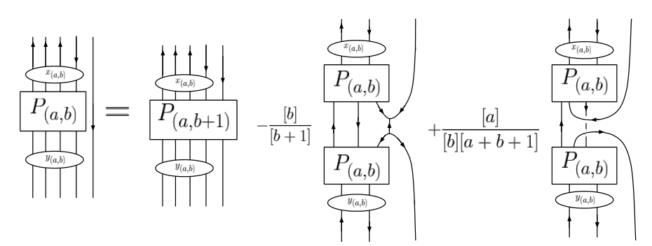
Then we see that this $3-$ term expansion gives us one term basically already in the form we desire, with the skein $x_{(a,b+1)}$ having a component that looks like $x_{(a,b)}$ with a disjoint strand immediately to the right. The next two terms we see have some skeins above and below identity tangles on fewer than $a+b$ strands, as $(a+1)+(b-2)$ and $(a-1)+b$ both satisfy this. This allows us to apply our inductive hypothesis on these ”internal” identity tangles. Then we can combine like terms, and in the process combining objects into a recursive construction for the $x$ and $y$ skeins. We note that since $a+b<m+n-1$ we have $a+b+1<m+n$ for all $(a,b)$. We also observe that the second half of our theorem holds as when applying this recursion to the lead term, we find the lead term in our new sum to be exactly $P_{(m,n)}$. ∎

Since

$$V_{h}C(a)V_{h}^{-1}=C(h(a)),$$

it suffices to show that for some $k$, $C(a)\neq C(h(a))$.

By the graph geodesic lemma $2.1$ above, there exists a handlebody $H$ bounded by $Y$ such that $a$ bounds an embedded disk in $H$ and $h(a)$ is a non-trivial graph geodesic with respect to a spine $S$ of $H$. This is illustrated below, where encircled region is exactly what is forbidden by the graph geodesic property.

Now let $Z(H)\in V(Y)$ be the vector determined by $H$ with the empty labelling, and $Z(H,h(a))$ the vector determined by the pair $(H,h(a))$ (where $h(a)$ is pushed into the interior of $H$). We have

$$C(a)(Z(H))=Z(H,a)=dZ(H)$$

as $a$ is taken to bound an embedded disk in $H$. It is also true that

$$C(h(a))(Z(H))=Z(H,h(a)),$$

meaning it suffices to show that $Z(H,h(a))$ is not a multiple of $Z(H)$.

Given a particular labelling $L=(l_{1},...,l_{n})$, where $l_{i}$ corresponds to a labelling of $v_{i}$ a vertex of the spine $S$, we construct a family of labellings $\{w_{L}\}$ of the spine $S$. For each edge $e$ of $S$, look at its dual disk $D$ and let $p$ be the number of times that $h(a)$ passes through $D$ where the orientation given by the orientation of boundary of $D$ and the orientation of $h(a)$ match, and $q$ the number of times $h(a)$ passes through $D$ with the opposite orientation. Up to the potential of including a pillow in a collar near this disk we have can think of $h(a)$ as passing through the disk as the $(p,q)$ identity tangle, $id(p,q)$ as defined above.

Then the edge $e$ is labeled by $(p,q)$. Finally define the complexity of a state vector as

$$m=\max(p_{e}+p_{f}+p_{g},q_{e}+q_{f}+q_{g}\}$$

where $e,f,g$ are three edges meeting at a vertex, and the max is over all vertices. Finally, pick a level $k\geq 2m$.

Let $\{b_{w_{L}}\}$ be the basis vectors for $V(Y)$ determined by the labellings $w_{L}$ of $S$. We claim that

$$Z(H,h(a))=\sum_{L}\lambda_{L}b_{w_{L}}+v,$$

where $\lambda_{i}\neq 0$ for all $i$, and $v$ consists of multiples of $b_{v}$ where $v$ is a label where

$$m_{e}+n_{e}<p_{e}+q_{e}$$

for each each $e$ of $S$. Applying Lemma $4.2$ we see that each edge label for $Z(H,h(a))$ can be factored in the desired manner. We are left to look at the vertex of each trivalent graph. This vertex is a skein in the triangle space of $(m_{1},n_{1}),(m_{2},n_{2})$ and $(m_{3},n_{3})$. Thus this skein is $\sum\lambda_{i}c_{i}$ where $c_{i}$ are the above basis vectors seen in Figure $6$. Now we claim as least one of the $\lambda_{i}$ is nonzero. As a skein, this trivalent vertex corresponds to the part of $h(a)$ which lives on a particular pair of paints, being pushed into the part of the handlebody bounded by this pair of pants. Combinatorially, we can describe each component of $h(a)$ by which boundary components it connects. The graph geodesic lemma tells us exactly that $h(a)$ never starts and ends at the same boundary component as seen in Figure 12. Then, introducing enough pillows, we are able to rearrange each strand that connects boundary components with the same orientation next to each other. This gives us exactly a realization of a basis element as described for the intertwiner spaces described above, as seen in Figure $6$ for example. As we can do this for each vertex and we will have a nonzero scalar pulled from each one. Therefore, $Z(H,h(a))$ cannot be a multiple of $Z(H)$ as it is not the empty labelling. ∎

If $h$ fixes all simple closed curves then $h$ must commute with all possible Dehn twists. As Dehn twists generate the mapping class group of any surface we have that $h$ must be in the center. Thus for any non-central $h\in\mathcal{M}$ that $h(a)$ is not isotopic to $a$, the main theorem follows from the above proposition. ∎

References

- [1] J. Andersen, Asyptotic Faithfulness of the Quantum Representations of the Mapping Class Group, Ann. Math., 163 (2006), 347-368.
- [2] M. F. Atiyah, The geometry and physics of knots, Cambridge University Press 1990.
- [3] C. Blanchet, Hecke algebras, modular categories and 3-manifolds quantum invariants, Topology 39 (2000) 193-223.
- [4] C. Blanchet, N. Habegger, G. Masbaum, and P. Vogel, Topological quantum field theories derived from the Kauffman Bracket, Topology 34(4) (1995) 883-927.
- [5] O. Davidovich, T. Hagge, and Z. Wang, On arithmetic modular categories, arXiv preprint arXiv:1305.2229 (2013).
- [6] M. Freedman, C. Nayak, K. Walker, and Z. Wang, On picture (2+1)-TQFTs, Topology and Physics, Nankai Tracts Math. 12, Hackensack, NJ: World Sci. Publ., 2008 19.
- [7] M. Freedman, K. Walker, Z. Wang, Quantum faithfully detects mapping class groups modulo center, Geom. and Topol. 6 (2002) 523-539.
- [8] V.F.R. Jones, Index for subfactors, Invent. Math. 72.1 (1983): 1-25.
- [9] L.H. Kauffman and S. L. Lins, Temperley-Lieb recoupling theory and invariants of 3-manifolds, Ann. Math. Study, Vol 134, Princeton University Press, Princeton (1994).
- [10] D. Kim, Jones-Wenzl idempotents for rank simple Lie algebras, Osaka J. Math., 44 (2007) 691-722.
- [11] G. Kuperberg, Spiders for rank Lie algebras, Comm. Math. Phys. 180 (1996), 109-151.
- [12] W. B. R. Lickorish, Skeins, SU(N) three-manifold invariants and TQFT, Comment. Math. Helv. 18(1) (2000)45-64.
- [13] G. Masbaum, Quantum representations of mapping class groups, Groupes et Géométrie (Journée annuelle 2003 de la SMF) (2003): 19-36.
- [14] T. Ohtsuki and S. Yamada, Quantum su(3) invariants via lienar skein theory, J. Knot Theory Ramifications 6 (1997) 373-404.
- [15] J. Roberts, Skeins and mapping class groups, Math. Proc. Cambridge Philos. Soc., Vol. 115. No. 01. Cambridge University Press, 1994.
- [16] N. Reshetikhin and V. G. Turaev, Invariants of 3-manifolds via link polynomials and quantum groups, Invent. Math. 103 (1991), no. 3, 547597.
- [17] N. Reshetikhin and V. G. Turaev, Ribbon graphs and their invariants derived from quantum groups, Comm. Math. Phys.127 (1990), no. 1, 126.
- [18] E. Rowell and Z. Wang, Mathematics of Topological Quantum Computing, Bull. AMS. (to appear), arXiv preprint arXiv:1705.06206.
- [19] E. Rowell, R. Strong, Z. Wang, On Classification of Modular Tensor Categories, Commun. Math. Phys. 292 (2009) 343-389.
- [20] L. C. Suciu, The SU(3) Wire Model, PhD thesis, Pennsylvannia State Univ., 1997.
- [21] V. G. Turaev, Quantum Invariants of Knots and 3-manifolds, de Gruyter Studies in Math. 18 Waltder de Gruyter & Co., Berlin, 1994.
- [22] Z. Wang, Topological quantum computation, CBMS Regional Conference Series in Mathematics, 112. American Mathematical Society, Providence, RI, 2010.
- [23] E. Witten, Quantum field theory and the Jones polynomial, Comm. Math. Phys. 121 (1989), no. 3, 351–399.