Local Master Equation for Small Temperatures
Abstract
We present a local Master equation for open system dynamics in two forms: Markovian and non-Markovian. Both have a wider range of validity than the Lindblad equation investigated by Davies. For low temperatures, they do not require coupling to be exponentially weak in the system size. If the state remains a low bond dimension Matrix Product State throughout the evolution, the local equation can be simulated in time polynomial in system size.
I Introduction
What are the effects in nonequilibrium dynamics where numerical simulation is more predictive than theory? A good example are nonlocal hops found during adiabatic evolution of a disordered system [1]. One can envision an experiment where this effect is measured in an ensemble of disordered systems. The results will be affected by interactions with the environment, so one needs to simulate open system dynamics to make any prediction of the results. Note that even the thermodynamics of disordered systems is hard for any analytic or numerical method, as it is a quantum version of classical glassy systems. These systems can encode NP-hard problems, and development of their theory is held back by intractability of a similar nature. A naive numerical study of their quantum behavior is bound to be exponentially hard in the system size. We believe that one can do better than that, at least for a special case of systems that are Many-body localized. In particular, we would wish to simulate quantum adiabatic annealing of such systems in the realistic setting that already has a lot of experimental data. [2, 3]
Here we are developing numerical tools to realize this idea. We formulate a new Master equation that has local structure and is appropriate for simulating dynamics of states that have local structure as well (such as Many-body localized states[4]). Previous work[5, 6, 7] often used the same approach without stating it in a form of a new equation. Other equations have been proposed[8, 9, 10], but the locality has not been stressed out. The traditional Lindblad master equation at finite temperature loses all the locality, so it becomes incompatible with modern Matrix-Product State methods[11, 12]. In this equation, a Rotating-wave approximation[13] is made that leads to its loss of locality. Terms containing are dropped from the Master equation with an assumption that .11 1 This is stated most explicitly in Zoller, page 88, about eqn. 3.6.67 Here are decoherence times, So the coupling to the bath should be weaker than typical level spacing, which for qubits goes as . For 10 qubits that would mean that . Thus we need times of decay at least in the units corresponding to the norm of local term in the Hamiltonian. This is grossly not true in systems like D-wave (time of decay is of order ).
Local Master Equation appears at the intermediate stage of the derivation of traditional Lindblad form[13]. We show that this equation possesses the same properties as the Lindblad one: positivity and Gibbs-preservation, but has wider range of applicability. Note that any nonequilibrium study in the literature that was using the traditional Lindblad Master equation can be redone with the new Master equation, and different results can be found. The goal of this paper is to provide a proof of concept using the simplest possible examples. Future applications include quantum adiabatic annealing, quantum thermodynamics[15] and stability proofs for open system evolution[16].
Local Master equation
The evolution of the density matrix of a system with the Hamiltonian interacting with the environment via a single operator is given by:
| (1) | |||
| (2) | |||
| (3) |
The filtered function is defined as:
| (4) |
where we can take either and . Taking will result in an evolution that does not preserve Gibbs state in general (which one partially fixes with counterterms), but it may preserve it in practice well enough. preserves the Gibbs state perfectly but has weaker error bounds due to other reasons.
The bath correlation function is defined to be:
| (5) |
where is a normalization constant chosen such that for convenience. One can then rescale to vary the strength of the noise. is the time-averaging window needed to restore positivity; in practice it is enough to set it to - norm of the local terms in the Hamiltonian.
Local Integral equation
An alternative form that has the largest range of applicability is:
| (6) | |||
| (7) | |||
| (8) | |||
| (9) |
Its time-averaged form can be found in Appendix A. The is an approximation to what’s actually needed to complete the integral to . Its value is:
| (10) |
In Section II we revisit the derivation of the above equation. In Section III we establish the Gibbs-preservation. In Section IV we focus on integral equation. Then we proceed to study applications of the derived methods in Section V. The theoretical bounds on error are presented in Section VI. We note the possibility of reduction from density matrices to states via the formalism of Quantum jumps in Section VII. Then in Section VIII we use the same formalism to convince ourselves in positivity of the evolution described by the new equation.
II Derivation of Master Equation
The typical derivation of the Master equation starts from
| (11) |
Take for simplicity where B is the bath operator, and both and are Hermitean. A general case can be treated in the same way. In the interaction picture the above equation has a formal solution
| (12) |
We can plug it into the equation:
| (13) |
So far all the steps were exact. So whatever integral operator stands in Eqn. (13), its application (e.g., by storing the result of the integration ) gives completely positive evolution. We now assume that at all times and take the trace. The positivity may be lost, but we operate under the assumption that it is still present. We will check that assumption when we arrive at the final form. We arrive to
| (14) | |||
| (15) |
Where is the bath correlation function to be discussed below. We did not assume anything about Markovianity. The above integral equation is hard to solve because one needs to store for all times. Indeed, the relative weight of time in the integral changes with according to . So there’s no trick to simulate the equation above, one just needs to honestly store a lot of ’s.
The Markovianity assumption comes into play here. We assume that over times when is not too small, the change in induced by the coupling to the bath is small. So one neglects it to the first order and replaces . After that, the integrals can be moved as below:
| (16) | |||
| (17) |
or better still, we may introduced filtered operator (it will be nonhermitean):
| (18) |
Final assumption is to send one of the limits to
| (19) |
The equation assumes a form:
| (20) |
Now by slight abuse of notation we define ”Shroedinger picture” filtered operator:
| (21) |
Since , the dependence on drops after shifting the range of integration:
| (22) |
Now in the Master equation, we can go to Shroedinger picture as well:
| (23) |
Note that is approximately local for decaying sufficiently fast due to Lieb-Robinson bound. Let’s now consider a more general bath . The equation takes the form:
| (24) |
where
| (25) |
and is the bath correlation between and . If those operators are local, one may use a bath that either have them completely independent, or such that correlations decay sufficiently fast. Then one can truncate to without introducing big error into equation. The radius of locality of the generators in master equations thus increases by only.
We derived a local Master equation. There were only three assumptions along the way:
- •
Separability, or Born approximation. One can check it by estimating the norm of the deviation from separability for any specific solution we find.
- •
Markovianity. If a solution is found, its characteristic timescale can be compared to the timescale of the bath
- •
Limits of integration. This one can mess up the first of the solution, so, e.g. something that starts as will start as , but after that time its effect is negligible.
There’re two problems with the equation above. First, it needs to be time-averaged over a small window to restore positivity, as discussed in Section VIII. Second, for appropriate thermal correlation function, the Gibbs state is not a fixed point of the evolution. We will need to extend the limits of the integration in to
| (26) |
to make Gibbs state an exact fixed point, as shown in Section III. However, we see the deviation of the fixed point from Gibbs state as a feature of our model, not a bug. Indeed, original equation on the total density matrix
| (27) |
preserves the total Gibbs state . It will preserve any diagonal in the total eigenbasis density matrix just as well. But it will not preserve any product state that is used in the Born approximation. So if we just look at this fact, we should not expect the Master equation to have a Gibbs fixed point. In Appendix C we find that the true fixed point is, instead, the reduced density matrix of the total Gibbs state:
| (28) |
so our equation captures the deviations from thermodynamical predictions on the interface between the system and the environment.
III Gibbs state fixed point
Often a desired property of the open system evolution is that the Gibbs state of an isolated system is a fixed point exactly. Even though it’s not very physical to require that (as we discussed above), we can get the state as a fixed point of the end equation using a certain trick.
Let’s see which terms of the equation favor which fixed point. The term preserves everything diagonal in the eigenbasis of the isolated system. The form of filtered operator
| (29) |
leads to the following terms
| (30) |
The is the bath spectral density defined as follows:
| (31) |
obeys the thermal law as shown in Appendix B. Note that can be expressed via as follows:
| (32) |
So if we had these limits of integration, we would only have in Master equation. The isolated Gibbs state is preserved by terms:
| (33) | |||
| (34) |
One may observe that they cancel each other as grouped.
Now is the remaining part.
| (35) |
It does not possess the thermal law, therefore terms will not preserve the Gibbs state
In traditional Lindblad Master equation at finite temperature, the RWA is applied (rotating-wave approximation), which amounts to requiring in the sum, and in terms like for offdiagonal . What remains of terms is
| (36) |
give offdiagonal contributions:
| (37) |
So we can include them in the dynamics as the lamb shift corrections to energies in Hamiltonian. But then there’s a mismatch: the Lindblad terms relax the system to Gibbs state of , but the dynamics is rotating with . One can rely on ”counter-terms” trick and include into from the start, and then neglect the difference in the Lindblad terms as it leads to kind of terms, and itself is , so the correction is fourth order in - smaller than the precision we care about for our equation.
It is left to the reader to decide whether to use counter-terms in a given specific case. Formally, Lamb shift should be included, but sometimes we want to study the specific Hamiltonian, so we may decide that it becomes such after contact with the bath has been established.
In our Local Master Equation, The Gibbs non-preserving corrections are not of the form anymore. But we note that we can approximate them by such, at least at low frequencies. Let’s get more specific.
in our case will be the Dawson function, and it generally varies on the scale of the bath width. Matrix elements of thus are not much different from matrix elements of within that band. And higher matrix elements can be suppressed in systems that have exponentially small for large energy change. So we make an approximation (an error of it is discussed in Section VI)
| (38) |
The second term then enters . Again, we can either simulate the dynamics of Lamb-shifted system, or assume that the opposite shift was present in the isolated system. In the end, the equation with exact Gibbs preservation that we use for Fig. 1-5 is the time-averaged version with all the counterterms gone:
| (39) | |||
| (40) | |||
| (41) |


IV Integral Equation
The Markovianity assumption required the bath time, which is at least (as shown in Appendix B), to be smaller than the time when any significant change in happened. Even more strict than that, we would want to simulate a significant change in , while constantly dropping contributions from its variation on the scale of . If those variations are , neglecting them throughour the dynamics leads to error . We know that since we want to see at least one half-life of the spin. So error . Which means . For the weak coupling, it seems to be an okay constraint but for a strong coupling we don’t have hopes to access big (small temperatures). And that constraint is assuming that our counterterms worked out, in fact the precision of those operations may pose even stricter constraints on . In particular, when we just use the ”lookforward” approximation in , it led to so .
In other words, for the problem at hand Markovianity is really out of question. One needs to see if there are non-Markovian integral equation that can still be simulated and possess the same nice properties: Gibbs-preservation, locality in some sense, and positivity.
The equation that we had before the Markovianity assumption was
| (42) |
(the interacting picture is used here). The Shroedinger picture gives:
| (43) |
The upper limit of the integral can now be changed to as long we are sufficiently far into the evolution. The closest we can get to Gibbs-preservation while maintaining accuracy is subtract :
| (44) |
The full time-averaged form is presented in Appendix A. Generally speaking, there are better ways to restore the Gibbs fixed point. One notes that any equation of the form
| (45) | |||
| (46) |
will preserve the Gibbs state exactly. For it is half-and-half combination of the Markovian and Non-Markovian equation. We do not know if such equations have any better bound on error if compared to original equation. Only in high- limit such bounds can be restored.
V Applications
We start with a single qubit pure state, and simulate the Eq. (39) for time and , which will be much bigger than what’s allowed by our approximations, but so we can see how the method performs in practice. The Hamiltonian is now:
| (47) |
and the . We expect decay to fixed point
| (48) |
and indeed observe it to at least 6 digits of precision. The now. The decay time is therefore expected to be . We observed a value around that, with some oscillations. (See Fig. 3)


We now (In Fig. 3,4,5) compare this evolution to an evolution with respect to traditional master equation:
| (49) | |||
| (50) | |||
| (51) |
where are eigenstates of the system Hamiltonian. The resulting evolution possesses the same features, however we find deviations of around in the oscillations before the equilibration.

Powder of sympathy
A good test for our ideas is the setup
| (52) |
Where is a bath operator. The relaxation of the excited state of spin is all due to the bottleneck , so we don’t expect to see anything up to exponential times. However, all our equations can produce faster relaxation if the bandwidth is broad enough, or , and the relaxation of has normal . This provides more constraints on the bandwidth: it shouldn’t be much bigger than or the energy scale of individual qubits, or it can lead to exponentially big bath fluctuations.
An interesting interpretation of this gedanken experiment is an old 17th century proposal of testing the effects of the ”Powder of Sympathy”, that can be found on the Wiki.
Locality
So far, we didn’t gain much by switching to local equation - one needs to calculate every matrix element of -by- matrix , which can easily take longer than the evolution itself. But note that the expression
| (53) |
only needs to be known up to some precision - accuracy of our evolution equation. So far we’ve made 3 (and more) approximations, now we’re just going to make another one by neglecting exponential tails of . We note that
| (54) |
and is the Hamiltonian truncated to a block around :
| (55) |
There are two contributions to :
| (56) |
for some such that . Here is the Lieb-Robinson velocity (essentially, norm of the Hamiltonian). The second contribution to error is then bounded by Lieb-Robinson bound:
| (57) |
where is a constant of order 1. What we derived is that we can approximate the timestep operators to a given error. In practice, we want where is the desired time we want to evolved the system for. For really short bath times the Lieb-Robinson bound may not even by tight. Anyways we can get away with ln blocks.
In this way, we get the size of the block to be at least (see decay time of the bath above). This illustrates the hardness of simulating low temperatures. Lower temperatures require us to compare energies at larger and larger scale.
Evolving MPS
Another question is whether implementing a difference scheme for local Master equation and Integral equation can be done locally. We assume that we only want to keep track of local operators. Then any state can be evolved for time with computation time exponential in (where is the Lieb-Robinson velocity). That is achieved, e.g. just by truncation to a block of size around the operator whose dynamics we wish to simulate. Also, any system can be evolved for time with computation time polynomial in and exponential in the system size. If one wishes to have simulation polynomial both in system size and in evolution, one needs to rely on approximate an ansatz such as Matrix Product States (MPS). There are ways to truncate the entanglement generated during evolution, and do so efficiently by looking at the state data only locally. Some of these truncation schemes will introduce a large error in practice. The choice of best truncation scheme is a topic of current research. Let’s assume that one chooses one of those schemes and is given a promise that it will succeed in approximating the evolution for a given system. After the efficient (poly-time) truncation, the evolution step is done. Its result can be represented as a sum of local operators acting on the MPS state. Then there are efficient ways of representing that sum as a new MPS.
Let’s illustrate that polynomial number of additions can be done on MPS states in poly-time. We act by a local operator on a state at . This adjusts the tensor . So we need to consider a sum of the original MPS and the adjusted one:
| (58) |
It’s all linear, the matrix multiplications are implied. We can directly add them now:
| (59) |
But then if we want to add a term with another adjusted, such nice form cannot be preserved anymore. However, if we assume that is small, then preserving this form will only make an error of order in any amplitude. We think that’s good enough.
So far, we glossed over how fine the memory of has to be stored for the calculation of integrals. Thanks to smoothing, we do not expect to have any oscillations with frequencies higher than . So that is a good interval to store values of . But then one needs to be careful when actually integrating, as as well as may contain rapid components. Anyways, can be truncated in time, and can be truncated in space. This gives a poly-time evolution-step for MPS-like system, as long as the long-range entanglement is truncated after every step. Of course, we do not have a good reason to truncate the entanglement - one never knows when it will come back and interfere on itself. But as long as the small error is promised to us, the faithful low-T simulations can be done in poly-time.
VI Error bounds
Let’s recap the timescales involved:
- •
- the characteristic timescale of the correlator of the bath.
- •
- temperature can also be thought of in the units of time
- •
- the timescale used for time-averaging
- •
- the decoherence time scale
- •
- inverse of typical internal frequency of our system
- •
- inverse of smallest level spacing
- •
- the desired evolution time, typically at least
Recall that has dimension of energy. Thus
| (60) |
has dimension of energy as well. Assuming:
| (61) |
we get
| (62) |
that has the right dimension. It has its maximum absolute value at :
| (63) |
and width for . We can make width even bigger for greater , but it does not get much smaller for smaller . Bigger width leads to weaker error bounds, so we fix . As a warmup, we bound the norm of :
| (64) |
we neglected the logarithm. The right-hand side of the equation is then of order:
| (65) |
So a change in will happen in time such that . We also note that the first of time are not very accurate for the Markovian equation, because integrals were replaced by . An integral equation does not suffer from that problem, if one keeps track of proper limits. So a meaningful comparison is possible only for . We can actually make our Markovian equation work in that regime as well, by introducing time-dependent in the beginning of evolution.
But let’s consider for simplicity. The rate of change in is , so the time-averaging replaces with something different by (In fact there are some cancellations, but considering them does not lead to a tighter bound). That difference leads to a deviation in the evolution of order:
| (66) |
In the Markovian equation, we also replaced on scales of order . In a similar way that leads to error
| (67) |
Note that for it’s more like , if one is careful in defining time-dependent . The Davies derivation does time-averaging as well, on a bigger scale . But it also drops some of the terms after it. The scale of those terms is
| (68) |
where the factor appears during the transition between bounds on individual matrix elements and bounds on the norm. is a dimension of a full system - we do not know how to do the truncation for the equation in Lindblad form. The minimum level spacing is . So even if there’s a tighter bound for norm transition, the factor exponential in system size still remains. Two terms depending on in the Davies equation are:
| (69) |
minimization of the error leads to
| (70) |
which is exponential in the system size.
Finally, we need to estimate the error of the Born approximation. Unlike the above estimates, we don’t really have a good control over it. So instead of an explicitly rigorous bound (like that in Davies paper), we just provide a proxy for it. We note that during the derivation, we introduced a nesting in the equation, by plugging in a formal solution:
| (71) |
We note that this formal solution that we plugged in does not exactly satisfy the Born approximation, even if that’s inside of it is Born. So one can imagine that by repeated nesting one improves the non-Born properties of the solution. Consider nesting two more times, and then taking the trace over bath. We get some equation on , that schematically can be written as follows:
| (72) |
Alternatively, we can get the equation of the same order by nesting the traced form that we used:
| (73) |
The two results will not coincide, even though they have the same order of operators. So the first order of error in Born approximation is
| (74) |
for , and for . It is essentially the same bound for . Maybe the special structure of the correction to Born approximation leads to cancellations that improve the above bound, but we do not investigate this further. We present two pictures of ranges of validity, one with the Born approximation proxy, and another without it (just other errors).
Conclusion: for 1 qubit with , the theoretical error bounds are summarized in the table:
| Born | Other errors | |
|---|---|---|
| Lindblad | ||
| Local ME | ||
| Integral equation |
These expressions are exactly the error rate per half-life . The is assumed. Most of the numerical factors are dropped for brevity, as bounds are not very tight in practice anyways.
Now for qubit system with , the biggest difference is that now Lindblad error bound grows exponentially with the dimension. We also assume that there are multiple coupled to independent baths acting on each qubit, which leads to some polynomial factors as well:
| Born | Other errors | |
|---|---|---|
| Lindblad | ||
| Local ME | ||
| Integral equation |
There is a truncation scheme outlined in Section V. If one uses local forms of , the for the dynamics is well approximated locally. can be replaced by for . We get the best error bounds for :
| Born | Other errors | |
|---|---|---|
| Local ME | ||
| Integral equation |
This is the error of local density matrices. We conclude that both of our equations avoid exponentially big factor, and locally even the polynomial factors. One should keep in mind that these theoretical bounds are not very tight, and only kick in for big systems though. For just one qubit, the equations track each other almost perfectly well outside the regime of validity prescribed by the bounds above. Fig. 6 shows the result of faithful simulation of the bath of 8 qubits and 1-qubit system. Both methods lose to finite-size effects very fast.
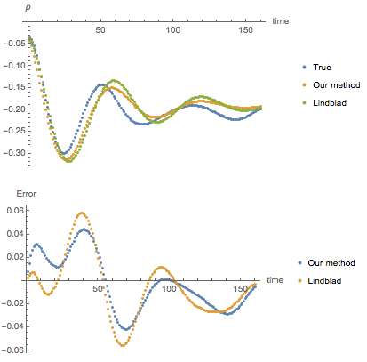
Now we will see what are the extra requirements on that come from demanding Gibbs-preservation requirement as in Section III.
The form of non-Gibbs preserving function for is:
| (75) | |||
| (76) |
It is a function with max height and characteristic width in . So the derivative is bounded by . A numerical investigation shows that one can plant on one of the extrema of Dawson function for . Then the second derivative is what gives the scale of Gibbs non-preserving terms at energy :
| (77) |
We note that for the analogous terms with are exponentially big, so we only need to worry about or so.
The difference is then bounded
| (78) |
If we only want to suppress terms, which would allow us to approximate well for , we can maintain control over .
The expression on the right for has minimum at :
| (79) |
The Fig. 7 shows a plot of magnitude of Gibbs non-preserving terms as a function of in units of . We also use time averaging with , but since it corresponds to high frequencies it doesn’t really matter.
We see that the magnitude is within 10 lines for , for . We also note that the picture is unchanged by rescaling , , and . If for some reason we decide to ignore the deviations outside the band, or ’s are such that suppress higher transitions, this is sufficient for Gibbs-preserving equation to be related to the true evolution.

VII To Stochastic Shroedinger eqn
Now we consider going from Master equation to Stochastic Shroedinger equation. Master equation is a linear differential equation on . We can write it concisely as
| (80) |
A formal solution is then
| (81) |
(for time-dependent Hamiltonian there are extra complications) These equations describe deterministic evolution of a -dimensional ”vector” . We can replace it by stochastic evolution of a -dimensional object . In some cases only a value of an observable is requested at the end of the evolution, so it may be faster to sample from stochastic evolution of -dimensional object than to run the full evolution of a -dimensional object. It is also more straightforward to implement the wavefunction evolution of the MPS than to implement the MPO evolution of the density matrix (there are plenty of problems with preserving Hermiticity etc. of locally in the latter).
Formally, the equivalence goes as follows: consider a matrix defined as . In case is a completely positive trace preserving map, is a proper density matrix on two copies of the system (-dimensional Hilbert space), as can be confirmed by acting with on one part of maximally mixed state in that Hilbert space. This gives us a way to check for positivity, if we’re afraid we’ve lost it in our approximations. is Hermitean (as long as equation on is invariant under Hermitean conjugation), so it can be diagonalized:
| (82) |
Where is diagonal matrix. Moreover, if positivity of the evolution holds, , so one can write
| (83) |
In indices, denote (Alternatively, we can use for , the result will be the same. In fact, there’s freedom in the choice of ). Note that We get
| (84) | |||
| (85) | |||
| (86) |
We’ve made the summation over indices explicit to stress out the point that our channel is a probabilistic sum:
| (87) |
The normalization of these operators may be all over the place. are just complex matrices. They can map a normalized state to something with norm less than or greater than one. The only constraint is that the total density matrix preserves its trace, so the norms should sum to over indices .
To use this form for computation, one first needs to represent , then sample from and choose a corresponding . Then pick an integer uniformly in and calculate . This unnormalized state is then used to calculate, e.g., expectation values of operators of interest.
| (88) |
These expectation values are averaged over random picks above.
| (89) |
One can easily check that
| (90) |
as it should be. Quite a lot of distributions are smooth enough so sparse sampling is sufficient.
Now we exploit the structure of our equation to come up with simple enough local operators . The time step is given by
| (91) | |||
| (92) |
The last two terms can be included as non-unitary part of the evolution:
| (93) | |||
| (94) |
Or, denoting the new, nonunitary evolution by ,
| (95) |
The right hand side needs to be represented as a sum of positive operators:
| (96) |
Note that the two terms in front of for completely arbitrary hermitean and nonhermitean
| (97) |
is not necessarily a positive operator. In other words, this operation on is not necessarily a positive map. Indeed, if and , then the operation acting on a valid density matrix results in a nonpositive operator .
So to find , consider an operator-state mapping defined as follows:
| (98) |
We arrive at the following form of :
| (99) |
We need to diagonalize it. Note that acts as zero outside the span of vectors in -dimensional space. So all we need to deal with is 3x3 matrix (if there are operators , then x). We can try to express the entries of the 3x3 matrix explicitly via the form of and the Gram matrix of inner products of . For that we will need to choose a basis, e.g. one vector along , second one perpendicular to it so lies in plane of these two, etc.
But we don’t need to work with the orthogonal basis. Instead, consider the eigenvalue equation:
| (100) |
Call the vectors by where . We assume they are linearly independent, and anyways
| (101) |
with unique choice of . Introduce the Gram matrix:
| (102) |
We arrive to the equation on vector :
| (103) |
here . So we have proven that non-Hermitean matrix has maximal number of independent eigenvectors. Moreover, the corresponding eigenvalues are real. We can just use the numerical procedure to deal with non-Hermitean matrix and it is guaranteed to find the full set.
Now using the values of ’s found numerically, we get
| (104) |
For the moment here we assume ’s will be positive which signals about the positivity of the map we’re trying to simulate. In practice we will need to extend to bigger matrices and drop some terms to achieve it, which is described in the next Section.
We translate back to jump operators by:
| (105) |
and
| (106) |
So the state should choose one of three paths with probabilities given by ’s and transform as:
| (107) |
Note that can be implemented by a finite-depth circuit. is usually local, so we only need to figure out how to achieve locality of , and then such jump can be calculated in -time for an MPS-like scheme.
Aside: if for many ’s we want to have jumps associated with each to be separate, we may use splitting of the identity trick to repeat the above for each with pieces of . That will add a requirement on the time step. However, having them all together does not lead to any problems.
VIII Positivity
The equation as it was derived originally is as follows:
| (108) |
The Eq. (108) is not guaranteed to give positive evolution. One may note, hovewer, that for , and the positivity is restored. Another way to restore it is dropping terms like:
| (109) |
which gives the standard ME in the Lindblad form, so explicitly positive.
One may ask what physical meaning is there in dropping the terms ? It can be achieved by smoothing the evolution. In equation
| (110) |
We can replace r.h.s. by r.h.s.. And then we still put . This averaging will make the terms if . For a random Hamiltonian of norm on qubits, the smallest , so we need to arrive at the usual Lindblad form. Of course it is not desirable to average our equation over such long timescale - no dynamics will be left. There are certain tricks one can do with Lieb-Robinson bound and truncation that may allow one to do better than this. We also note that Lindblad form is guaranteed to be positive, whereas our equation does not. Positivity is restored for some , so this is a way to tweak our equation if it’s not positive from the start in a given special case.
We find out that such evolution has third eigenvalue of the corresponding (via channel-state duality) always negative. We fight that by time averaging the interaction part. We take a simple 3 point average:
| (111) | |||
| (112) | |||
| (113) |
here is a new time scale, in practice it is enough to choose . For and and (something generic, but relevant for the D-wave problem) one obtains as the averaging time when the negative eigenvalue becomes the 4th. Same works for 2,3,5 qubit system with random chain Hamiltonians.
We note that such is a big achievement of our method, the original Lindblad-Davies derivation needed the inverse smallest level spacing.
The way the positivity is checked is by investigating a -by- operator, which actually has only -by- matrix of nontrivial components (one for identity and two for each point in our averaging):
| (114) | |||
| (115) | |||
| (116) |
here on the two copies of a system, and . The bra-ket notation as applied to operators is somewhat misleading. The difference between the operator space and the quantum state space is that there’s no good inner product on operator space. The above bra-ket imply the Tr inner product, but it doesn’t work out in quite the same way as the inner product for states.
A more mathematically correct way of posing the question is that is a quadratic form . It takes as input operators in span of as one argument, their conjugates as another, and spits out a (generally complex) number. The quadratic form is completely defined by the Eq. (114). For example, . The value of on any two operators can be expressed via linearity. Anything outside the span of our seven vectors is set to zero. If some of the vectors are linearly dependent, one chooses a basis. The resulting form output on two vectors is invariant with respect to a choice of basis.
Then one can ask to make this quadratic form diagonal. Once it’s done, one investigates the values on the diagonal and checks for their positivity.
What we do is finding eigenvalues of instead. Note that if , then we arrive to equation on and :
| (117) |
where is the matrix of inner products in the Tr sense. One can rigorously derive the above equation. Consider acting by the evolution map on the maximally mixed state of two copies of the system (that is a pure state as a whole). The resulting density matrix is hopefully positive and surely Hermitean, so it has its eigenvalues. Its eigenvalue equation leads to Eq. (117).
So we are choosing the averaging timestep so that negativity of matrix for our actual map is not too big. Where does the negativity come from? Each 2-by-2 matrix is bound to have a negative eigenvalue. The eigenvalues are (assuming a good normalization) if and if . Finite temperatures are all somewhere in between these two cases. Now adding the term may in principle lift these two, but in practice overlap between and is too small to do anything. So we do the averaging, going to 7-by-7 matrix. Now there are 7 eigenvalues, 6 of which form a block relating to . This block for small will still have two leading eigenvalues of different signs with the same magnitudes as before, as well as some very small eigenvalues. Raising increases the small ones until they overtake the negative one. That is the moment when we consider that our dynamics is positive enough. In practice it is achieved by for norm of terms in the Hamiltonian . One can write down an explicitly positive evolution by keeping the above three eigenvaluese at this and dropping the rest, but the error one makes while keeping all the terms is small enough. And using the original form with and is so much simpler.
Numerical investigation
The matrix has small negative eigenvalues . One needs to be careful as the basis is not orthonormal, large norms may appear. The hamiltonian is:
| (118) |
The . Our investigation of positivity will apply to each portion of the noise separately, for small enough . is taken to be .
With that, we evaluate the eigenvalues of for for different .


It is an avoided crossing, so one can convince oneself that the level that used to be negative passes all the zeros and becomes positive.
Acknowledgements.
The author is thankful to Alexei Kitaev, John Preskill and Leonid Pryadko for useful comments and discussion. E.M. carried out some of this work while supported by the Simons Foundation.Appendix A Exact time-averaging
Let’s first formulate the steps of time averaging of a linear differential equation that can lead to sum of , and terms that appears in the Local Master Equation. We start with the equation
| (119) |
where contains rapidly changing terms. If we naively replace it by our desired equation
| (120) |
Then the difference becomes over 1 half-life. As contains both rapid and slow terms, we don’t expect to be small. It will be of order - the typical timescale of the hamiltonian. So
| (121) |
In our case and for 1 spin, which is too much of an error. A thermal state differs from maximally mixed state by roughly that much for . We want to do better than that. We note that will also contain rapid terms. We don’t intend to keep track of oscillations faster than frequency , so we may as well consider evolution of the averaged density matrix
| (122) |
Note that the difference is small at all times:
| (123) | |||
| (124) |
Now we will derive the equation on , and see that it differs from a desired Markovian equation by a small amount. The difference between true and the solution of our equation will be , which is tolerable for small .
| (125) | |||
| (126) | |||
| (127) | |||
| (128) | |||
| (129) | |||
| (130) | |||
| (131) | |||
| (132) |
Here range in . The first term in the last line is the desired equation, the other are of order . For a total evolution time such that we get error .
So if we find a solution of the above equation we are guaranteed that the solution of the original equation is within of it. In this way, we have proven that there is a tighter bound on that we naively expected. Same applies for Heisenberg and , because the error term just gets unitary rotated, but does not increase in the norm.
Of course, the above trick can also be applied to the integral time averaging .
Now let’s try to extend this method of deriving equation on to the integral equation. There’s a freedom how to do that. We want all the ’s involved to be within , which can be done by shifts in . An equation will then contain terms like (in the Heisenberg picture):
| (133) |
which contain shifted to prevent looking in the future, as well as terms
| (134) |
we can remove from for the sake of symmetry of the expression - that does not lead to a significant error. The counterterms also get their time-averaged version looking just like the Local Master Equation.
| (135) | |||
| (136) | |||
| (137) | |||
| (138) | |||
| (139) | |||
| (140) | |||
| (141) | |||
| (142) | |||
| (143) |
Appendix B Bath correlation
The master equation used the following correlation function of the environment:
| (144) |
and its complex conjugate if is a Hermitean operator.
If it happens that is purely real for all , then the bath is infinite temperature. The imaginary part is necessary for finite temperature steady state.
By a straightforward use of eigenbasis of the bath, we get
| (145) | |||
| (146) |
Where
| (147) |
Note that . Also, consider two delta functions, corresponding to and , with amplitudes and correspondingly. The magnitude of -function in at is times the magnitude at . This holds for all contributing functions, thus it holds for appropriate smooth version of in the thermodynamic limit:
| (148) |
So we can take any that is positive and satisfies Eq. (148). From the derivation of the Master equation, there’s an extra requirement that decays with sufficiently fast. Besides that, can be any real positive function.
There’s one particularly simple choice . Let’s calculate the corresponding decay time, as this is the one we will use in the numerics.
| (149) | |||
| (150) |
We see that the decay time is:
| (151) |
So we need both high and broad (fast) bath for the derivation of Markovian master equation to be valid.
Appendix C True Fixed Point
Derivation of fixed point equations
| (152) | |||
| (153) |
After splitting and denoting
| (154) |
the correlation functions can be related by analytic continuation in the following way
| (155) | |||
| (156) | |||
| (157) |
We also note that thanks to the Gibbs factor the possesses the property
| (158) |
Now let’s express :
| (159) |
Now
| (160) |
where small was added to keep track of the pole shifts below.
| (161) |
Now the integral splits into the principal value and the pole:
| (162) |
so
| (163) |
Now let’s look at the Gibbs preservation. The environment-induced part of the equation is as follows:
| (164) |
We need to see what it does to Gibbs state. First investigate the component of that is proportional to . Note that the Hermitean conjugation flips the sign of the energy:
| (165) |
We arrive at
| (166) |
we group the first and the last term, and the middle two:
| (167) |
One may observe that they cancel each other as grouped:
| (168) | |||
| (169) |
because
| (170) |
where we have used the special property of spectral density. So the equation with just terms would preserve the isolated system Gibbs state. Now let’s derive the remaining terms containing principal value integrals. For brevity, we denote
| (171) |
so the part of we care about is (let’s call it )
| (172) |
Now the full expression for Hermitean conjugation can be written concisely:
| (173) |
We calculate the remaining part of the evolution of the Gibbs state:
| (174) |
this part does not, in general, vanish. We will see how it contributes to the true fixed point below.
True Gibbs preservation
The Integral equation decays to the same fixed point as the Markovian equation, as it should because fixed point condition involves time-independent :
| (175) |
In perturbation theory, that fixed point is shifted by terms away from the isolated system Gibbs distribution. We do not know if there’s a general bound on the size of those terms, and thus on the validity of the perturbative approach. But we will see that it is valid at least in a sense that the matrix element deviations are small under not very restrictive conditions. For a perturbative calculation, one notes that commutes with the Hamiltonian, and that can be dropped in the decay term in the first order calculation:
| (176) |
We have already done the calculation for the terms on the right:
| (177) |
In the first order, the fixed point has the same diagonal (one can easily see that by checking that terms cancel from the above sum). The offdiagonal contributions will be (new signs!):
| (178) |
As usual perturbation theory calculation, it doesn’t behave well at , and degenerate perturbation theory should be used. We note that neither of cases () provides a good bound on in general, but under certain assumptions it is small.
More specifically, for a system of size with minimal spacing we can bound the at least as:
| (179) |
using the above formula.
Another thing one may wish to prove is that , if not small, is at least local in some sense. And indeed, if the system decays at a good rate, the equation itself is the proof that it is local. For systems that do not relax well due to big memory times the naive evolution with our equation does not prepare a thermal state, neither we expect it to be related approximately by a local superoperator to the original one.
Now let’s compare our fixed point to the true reduced density matrix
| (180) |
the expansion is not neccessarily valid, because norms for do not have to be of the same order as . There may be huge factors in them. Maybe if one carefully investigates this expression, one will find suppression anyways, because of the factors. There don’t seem to be an easy counterexample.
Surprisingly, the above formula is exactly the fixed point of our equation! So to this order where is the same as one found by perturbation theory of the fixed point condition. It also helps to figure out the fate of apparent zero in the denominator in that equivalence. In fact, one of the integrals turns out to give that:
| (181) |
where . Then two terms in the numerator lead to different summands in expression for . In other words, appropriate grouping of the term should remove the apparent pole.
So we are convinced that our equation (both Markovian and Integral) has true reduced density matrix tr as a fixed point. There’s nothing more physical than that. If one demands the Gibbs state of , we can’t really guarantee to be close to it in the norm. Every matrix element will be close to the one of isolated system as (if we forget about the pole). Neither we know how to introduce counterterms that will restore it as an exact fixed point.
We will present a suggestion that works for special systems - many-body localized ones. There one indeed can hope for corrections to be small and local. A little bit more generally, one may be able to bound the correction for any locally generated fixed point (the one that can be disentangled by local operations across any cut).
The derivation
| (182) |
where is an analytic continuation of . Explicitly we had:
| (183) | |||
| (184) |
Let’s do the same eigenstate decomposition on the system now:
| (185) |
Recall that in our target formula
| (186) |
The non-principal value part corresponding to the pole is also there, but it cancels due to thermal law. We will try to collect the above expressions in the result of integration over . First we shift to new variables and . The integrals become:
| (187) | |||
| (188) | |||
| (189) | |||
| (190) |
It will be neccessary to use the property : (recover factors!)
| (191) | |||
| (192) | |||
| (193) | |||
| (194) | |||
| (195) | |||
| (196) | |||
| (197) |
Note that we implied the principal value because the terms with cancel due to thermal law. The signs are wrong for that though… Maybe there are strategic that fix it - I don’t know how to keep track of pole bypass directions. The final answer for the correction is:
| (198) |
Let’s look at the other derivation -
the answer we got there was
| (199) |
Indeed perfect coincidence.
In fact the above calculation of equivalence of fixed point to reduced Gibbs state only applies for . For the reduced Gibbs state expression has to be used as if in the limit
| (200) |
That limit indeed exists, as can be seen from the expression directly:
| (201) |
The numerator is zero at and its first derivative gives the following limit:
| (202) |
The last term also appears if one does the counterterm trick in the traditional Lindblad equation. We do not know of the interpretation of the first two. doesn’t satisfy the thermal law, so they don’t cancel.
But our first order fixed point condition is trivially satisfied at , so any change in diagonal elements of preserves the condition to that order. We assumed that there are no degeneracies in the Hamiltonian for simplicity, so we can call the diagonal. In higher order we find a fixed point of the diagonal to precision, and offdiagonal elements to precision. The fixed point of traditional Lindblad equation can be changed by amount by introducing appropriate counterterms, so it can be made to be exactly the diagonal of reduced Gibbs state. The offdiagonal fixed point is zero for Lindblad. The fixed point without counterterms is just of isolated system.
In our case, there are offdiagonal terms in the fixed point, so they will shift the diagonal. Specifically, one can denote a superoperator:
| (203) |
The second order perturbation theory for fixed point is then:
| (204) |
where where is already found in the first, and is the to be determined. By taking elements of the above equation, we kill the contributions of :
| (205) |
or
| (206) |
So we just need to invert the operator that maps diagonal to diagonal. But that is exactly the relaxation part of the traditional Lindblad equation! It has zero eigenvalue corresponding to , which is expected from perturbation theory (we won’t find meaningful corrections to the amplitude of zeroth order state). But in the subspace of other eigenvectors we can invert this matrix:
| (207) |
or in components:
| (208) |
where are eigenvectors of the Markov process. This form is a bit concerning because can be arbitrarily big, but we remember from our original estimates that if diagonal deviates more than from the Gibbs state, the first order condition will not be able to balance them anymore, so fixed point can’t be further than that. So we expect that by appropriate counterterms we can remove this correction and restore the true fixed point diagonal of reduced Gibbs state (or isolated Gibbs state, if one so desires).
References
- [1] V. Khemani et al. Nonlocal adiabatic response of a localized system to local manipulations. Nature Physics, 11:560–565, 2015.
- [2] N. G. Dickson et al. Thermally assisted quantum annealing of a 16-qubit problem. Nat Commun., 4:1903, 2013.
- [3] M. A. Schmidt et al. Using thermal boundary conditions to engineer the quantum state of a bulk magnet. PNAS, 111:3689–3694, 2014.
- [4] J. Imbrie. On many-body localization for quantum spin chains. J. Stat. Phys., 163:998, 2016.
- [5] R.P Feynman and F.L Vernon Jr. The theory of a general quantum system interacting with a linear dissipative system. Annals of Physics, 24:118–173, 1963.
- [6] A.O. Caldeira and A.J. Leggett. Path integral approach to quantum brownian motion. Physica A: Statistical Mechanics and its Applications, 121:587–616, September 1983.
- [7] I. Martin M. B. Hastings and D. Mozyrsky. Quantum dynamics in non-equilibrium strongly correlated environments. Phys. Rev. B, 68:035101, 2003.
- [8] T. Albash et al. Quantum adiabatic markovian master equations. New Journal of Physics, 14, December 2012.
- [9] Z. Biharyb D. A. Lidar and K.B. Whaley. From completely positive maps to the quantum markovian semigroup master equation. Chemical Physics, 268, 2001.
- [10] A. Shabani and D. A. Lidar. Completely positive post-markovian master equation via a measurement approach. Phys. Rev. A, 71, 2005.
- [11] Ulrich Schollwöck. The density-matrix renormalization group in the age of matrix product states. Annals of Physics, 326:96–192, January 2011.
- [12] R. Orús and G. Vidal. Infinite time-evolving block decimation algorithm beyond unitary evolution. Phys. Rev. B, 78:155117, October 2008.
- [13] E. B. Davies. Markovian master equations. Comm. Math. Phys., 39:91–110, 1974.
- [14] This is stated most explicitly in Zoller, page 88, about eqn. 3.6.67.
- [15] E. Geva and R. Kosloff. A quantum-mechanical heat engine operating in finite time. a model consisting of spin-1/2 systems as the working fluid. The Journal of chemical physics, 96:3054–3067, 1992.
- [16] Toby S. Cubitt et al. Stability of local quantum dissipative systems. Communications in Mathematical Physics, 337:1275–1315, 2015.