跳到论文正文
W Papers独立论文阅读器 arXiv:1611.04113 论文正文 计算阅读时间 · 0%
引用这篇论文根据当前论文元数据生成,正式投稿前建议核对。


License: arXiv.org perpetual non-exclusive license
arXiv:1611.04113v2 [math.NA] 21 Nov 2016

A splitting method for the augmented Burgers equation

L. I. Ignat, A. Pozo Address: Liviu I. Ignat Institute of Mathematics “Simion Stoilow” of the Romanian Academy
21 Calea Grivitei Street
010702 Bucharest
Romania.
Email address: liviu.ignat@gmail.comWeb page: http://www.imar.ro/~ lignat Address: Alejandro Pozo CBT - Innovalia
Carretera de Asua 6, E-48930 Las Arenas - Getxo, Basque Country - Spain. and BCAM - Basque Center for Applied Mathematics
Alameda de Mazarredo 14, E-48009 Bilbao, Basque Country - Spain.
Email address: alejandropozo@gmail.com
Date: August 24, 2026
Abstract.

In this paper we consider a splitting method for the augmented Burgers equation and prove that it is of first order. We also analyze the large-time behavior of the approximated solution by obtaining the first term in the asymptotic expansion. We prove that, when time increases, these solutions behave as the self-similar solutions of the viscous Burgers equation.

1. Introduction

In this paper we consider a splitting method for the following augmented Burgers equation:

(1.1) {ut−(u22)x=ux​x+K∗u−u+ux,(t,x)∈(0,∞)×ℝ,u⁡(0,x)=u0​(x),x∈ℝ,\begin{cases}u_{t}-\left(\frac{u^{2}}{2}\right)_{x}=u_{xx}+K*u-u+u_{x},&(t,x)\in(0,\infty)\times\mathbb{R},\\ u(0,x)=u_{0}(x),&x\in\mathbb{R},\end{cases}

where K⁡(z)=e−z​χ(0,∞)K(z)=e^{-z}\chi_{(0,\infty)}. This model has been introduced in the context of the analysis of the sonic-boom phenomenon to reproduce the propagation of the sound waves produced by supersonic aircrafts from their near-field down to the ground level [5, 16, 17].

New trends in aerospace engineering have started to use nonlinear physical models to characterize this phenomenon, in order to be capable of building efficient supersonic civilian airplanes that can avoid such strident noise. We refer the reader to [2] for a detailed survey on the topic. In this paper we focus on the augmented Burgers equation, which was initially developed by Cleveland [5] and later adopted by Rallabhandi [16, 17].

Let us now explain the general setting from where model (1.1) appears. The nonlinear equation that models the sonic-boom phenomenon is given by

(1.2) ∂P∂σ=P​∂P∂τ+1Γ​∂2P∂τ2+∑νCν​11+θν​∂∂τ​∂2P∂τ2−12​G​∂G∂σ​P+12​ρ0​c0​∂(ρ0​c0)∂σ​P,\frac{\partial P}{\partial\sigma}=P\frac{\partial P}{\partial\tau}+\frac{1}{\Gamma}\frac{\partial^{2}P}{\partial\tau^{2}}+\sum_{\nu}C_{\nu}\frac{1}{1+\theta_{\nu}\frac{\partial}{\partial\tau}}\frac{\partial^{2}P}{\partial\tau^{2}}-\frac{1}{2G}\frac{\partial G}{\partial\sigma}P+\frac{1}{2\rho_{0}c_{0}}\frac{\partial(\rho_{0}c_{0})}{\partial\sigma}P,

where P=P⁡(σ,τ)P=P(\sigma,\tau) is the dimensionless perturbation of the atmosphere pressure distribution. The covered distance σ\sigma and time of the perturbation τ\tau are also dimensionless. The operator appearing in the summation, corresponding to the molecular relaxations, is defined by:

(1.3) 11+θ​∂∂τ​f​(τ)=1θ​∫−∞τe(ξ−τ)/θ​f​(ξ)​𝑑ξ=Kθ∗f⁡(τ),\frac{1}{1+\theta\frac{\partial}{\partial\tau}}f(\tau)=\frac{1}{\theta}\int_{-\infty}^{\tau}e^{(\xi-\tau)/\theta}f(\xi)d\xi=K_{\theta}*f(\tau),

where θKθ(θ⋅)=K(⋅)\theta K_{\theta}(\theta\ \cdot)=K(\cdot). Typically, two relaxation modes are considered (one for Oxygen molecules and another one for Nitrogen molecules), each of them with their corresponding dimensionless relaxation time θν\theta_{\nu} and dispersion parameter CνC_{\nu}. Γ\Gamma is a dimensionless thermo-viscous parameter and function G≡G⁡(σ)G\equiv G(\sigma) denotes the ray-tube area. Density ρ0≡ρ⁡(σ)\rho_{0}\equiv\rho(\sigma) and speed of sound c0≡c0​(σ)c_{0}\equiv c_{0}(\sigma), both closely related to the altitude of the flight, determine the atmosphere conditions. We refer to [5] for the complete formulation and setting-up of this model. In this paper we analyze the particular model (1.1) that can be obtained from (1.2) by choosing p0p_{0}, c0c_{0} to be constant, Γ=1\Gamma=1 and a single relaxation phenomenon with cν=θν=1c_{\nu}=\theta_{\nu}=1.

Industrial applications like the aforementioned sonic-boom phenomenon, in which approximate solutions for large time are required, need a careful numerical treatment. A good understanding of the behavior of the solutions in these extended regimes, both in continuous and discrete settings, is necessary in order to be able to simulate them accurately. In that sense, equation (1.1) has already been analyzed in [11]. The authors have obtain the asymptotic profile of the solutions of (1.1) as time goes to infinity. Moreover, they propose a semi-discrete scheme that is capable of mimicking the large-time dynamics of the continuous system. This issue needs to be treated carefully, since numerical schemes with an acceptable accuracy in short-time intervals can completely disturb the large-time behavior of solutions when the numerical viscosity dominates the physical one [12]. However, solving (1.1) by discretizing the convolution can be computationally expensive. In this paper we set up the framework to empower the use of splitting methods to solve the equation more efficiently. Let us mention that these techniques have already been used in [5, 16, 17] in the context of the sonic-boom phenomenon. Various versions of this method have also been developed, for instance, for the nonlinear Schrödinger, Korteweg-de Vries, Boltzmann… (see [8] and the references therein) and, more recently, for the nonlocal Fowler equation [3].

The basic idea behind operator splitting methods is that the overall evolution operator can be formally written as a sum of evolution operators for each term appearing in the model. In other words, one separates the complete system into a set of simpler sub-equations, for which more practical algorithms are available. Once we successively solve these sub-equations, their solutions are put together to compute the complete solution of the model. We refer to [8] for a more detailed introduction on operator splitting methods.

Let us remark that the analysis performed in this paper can be extended to any kernel K∈L1​(ℝ,1+|x|2)K\in L^{1}(\mathbb{R},1+|x|^{2}) by replacing the term K∗u−u+uxK\ast u-u+u_{x} adequately. The analysis we present here for K⁡(z)=e−z​χ(0,∞)K(z)=e^{-z}\chi_{(0,\infty)} is the same for any kernel having the mass and the first moment equal to one:

(1.4) ∫ℝK⁡(z)​𝑑z=∫ℝK⁡(z)​z​𝑑z=1.\int_{\mathbb{R}}K(z)dz=\int_{\mathbb{R}}K(z)zdz=1.

We introduce the following Trotter formula for the augmented Burgers equation (1.1). Let XtX^{t} be the evolution operator associated with

(1.5) {vt=K∗v−v+vx,(t,x)∈(0,∞)×ℝ,v⁡(t=0,x)=v0​(x),x∈ℝ,\begin{cases}v_{t}=K*v-v+v_{x},&(t,x)\in(0,\infty)\times\mathbb{R},\\ v(t=0,x)=v_{0}(x),&x\in\mathbb{R},\end{cases}

and YtY^{t} the one corresponding to

(1.6) {wt−(w22)x=wx​x,(t,x)∈(0,∞)×ℝ,w⁡(t=0,x)=w0​(x),x∈ℝ.\begin{cases}w_{t}-\left(\frac{w^{2}}{2}\right)_{x}=w_{xx},&(t,x)\in(0,\infty)\times\mathbb{R},\\ w(t=0,x)=w_{0}(x),&x\in\mathbb{R}.\end{cases}

We consider the flow ZtZ^{t} defined by

(1.7) Zt=Xt​Yt.Z^{t}=X^{t}Y^{t}.

The aim is to approximate the flow StS^{t} given by (1.1) by alternating both operators; that is, for small Δ​t>0{\Delta t}>0 and positive integers nn we want to analyze whether

Sn​Δ​t​u0=u⁡(n​Δ​t)≈(ZΔ​t)n​u0=(XΔ​t​YΔ​t)n​u0.S^{n{\Delta t}}u_{0}=u(n{\Delta t})\approx(Z^{\Delta t})^{n}u_{0}=(X^{\Delta t}Y^{\Delta t})^{n}u_{0}.

Subsequently we denote Zn​Δ​tZ^{n{\Delta t}} instead of (ZΔ​t)n(Z^{\Delta t})^{n} for the sake of clarity of the notation.

The first result of this paper is given in the following theorem. It confirms that the splitting (1.7) is first-order accurate for H2​(ℝ)H^{2}(\mathbb{R})-solutions. For practical issues we also consider the case of H1​(ℝ)H^{1}(\mathbb{R})-solutions.

Theorem 1.1.

Let r∈{1,2}r\in\{1,2\}. For any u0∈Hr​(ℝ)u_{0}\in{H^{r}(\mathbb{R})} and for all T>0T>0, the following hold:

‖Zn​Δ​t​u0−u⁡(n​Δ​t)‖L2​(ℝ)≤C⁡(T,‖u0‖H1)​‖u0‖Hr​(ℝ)2​(Δ​t)r/2\left\|Z^{n{\Delta t}}u_{0}-u(n{\Delta t})\right\|_{L^{2}(\mathbb{R})}\leq C(T,\|u_{0}\|_{H^{1}})\|u_{0}\|_{H^{r}(\mathbb{R})}^{2}({\Delta t})^{r/2}

and

‖Zn​Δ​t​u0‖Hr​(ℝ)≤C⁡(T,‖u0‖L2​(ℝ))​‖u0‖Hr​(ℝ),\left\|Z^{n{\Delta t}}u_{0}\right\|_{H^{r}(\mathbb{R})}\leq C(T,\|u_{0}\|_{L^{2}(\mathbb{R})})\|u_{0}\|_{H^{r}(\mathbb{R})},

for all Δ​t∈(0,1){\Delta t}\in(0,1) and for all n∈ℕn\in\mathbb{N} such that 0≤n​Δ​t≤T0\leq n{\Delta t}\leq T.

The second result of this paper concerns the first term in the asymptotic expansion of the approximate solution Zn​Δ​t​u0Z^{n\Delta t}u_{0}. To be more precise let us define tn=n​Δ​tt_{n}=n{\Delta t} and tn+1/2=(n+12)​Δ​tt_{n+1/2}=(n+\frac{1}{2}){\Delta t} for every n∈ℕ∪{0}n\in\mathbb{N}\cup\{0\} and the function uΔu^{\Delta} by

(1.8) uΔ​(t,x)={Y2​(t−tn)​Zn​Δ​t​u0​(x),t∈[tn,tn+1/2),x∈ℝ,X2​(t−tn+1/2)​YΔ​t​Zn​Δ​t​u0​(x),t∈[tn+1/2,tn+1),x∈ℝ.u^{\Delta}(t,x)=\begin{cases}Y^{2(t-t_{n})}Z^{n{\Delta t}}u_{0}(x),&t\in[t_{n},t_{n+1/2}),\ x\in\mathbb{R},\\ X^{2(t-t_{n+1/2})}Y^{{\Delta t}}Z^{n{\Delta t}}u_{0}(x),&t\in[t_{n+1/2},t_{n+1}),\ x\in\mathbb{R}.\end{cases}

Observe that for any n≥0n\geq 0, uΔ​(tn)=Zn​Δ​t​u0u^{\Delta}(t_{n})=Z^{n{\Delta t}}u_{0}. By construction and the properties of XtX^{t} and YtY^{t}, we will have that for any u0∈Lp​(ℝ)u_{0}\in L^{p}(\mathbb{R}), 1≤p<∞1\leq p<\infty, uΔu^{\Delta} defined by (1.8) satisfies uΔ∈C⁡([0,∞),Lp​(ℝ))u^{\Delta}\in C([0,\infty);L^{p}(\mathbb{R})) for any 1≤p≤∞1\leq p\leq\infty. The behavior of uΔu^{\Delta} as t→∞t\to\infty, so the one of Zn​Δ​t​u0Z^{n{\Delta t}}u_{0}, follows from a scaling argument. Indeed, the following result confirms that the Trotter formula (1.7) for the augmented Burgers equation (1.1) preserves the large-time behavior obtained in [11].

Theorem 1.2.

For any u0∈L1​(ℝ)∩L∞​(ℝ)u_{0}\in L^{1}(\mathbb{R})\cap L^{\infty}(\mathbb{R}) and for all p∈[1,∞)p\in[1,{\infty)}, it holds that

(1.9) t12​(1−1p)​‖uΔ​(t)−uM​(t)‖Lp​(ℝ)→∞,as ​t→∞,t^{\frac{1}{2}(1-\frac{1}{p})}\left\|u^{\Delta}(t)-u_{M}(t)\right\|_{L^{p}(\mathbb{R})}\to\infty,\quad\mbox{as }t\to\infty,

where uM​(t,x)=t−12​fM​(x/t)u_{M}(t,x)=t^{-\frac{1}{2}}f_{M}(x/\sqrt{t}) is the self-similar profile of the following viscous Burgers equation

(1.10) {ut=(u22)x+2​ux​x,(t,x)∈(0,∞)×ℝ,u⁡(0,x)=M​δ0,x∈ℝ.\begin{cases}u_{t}=\left(\frac{u^{2}}{2}\right)_{x}+2u_{xx},&(t,x)\in(0,\infty)\times\mathbb{R},\\ u(0,x)=M\delta_{0},&x\in\mathbb{R}.\end{cases}

where MM is the mass of the initial data.

Let us recall, see for example [1], that equation (1.10) has a unique solution of the form u(t,x)=t−1/2fM(x/t1/2)u(t,x)=t^{-1/2}f_{M}(x/t^{1/2}) where the profile fMf_{M} is smooth, decays as |x|→∞|x|\rightarrow\infty and has mass MM and constant sign.

Moreover, the above theorem provides information about the asymptotic behavior of the approximation Zn​Δ​tZ^{n{\Delta t}} since uΔ​(n​Δ​t)=Zn​Δ​t​u0u^{\Delta}(n{\Delta t})=Z^{n{\Delta t}}u_{0}. In fact, for any fixed Δ​t\Delta t and any 1≤p<∞1\leq p<\infty we have

(n​Δ​t)12​(1−1p)​‖Zn​Δ​t​u0−uM​(n​Δ​t)‖Lp​(ℝ)→∞,as ​n→∞.(n{\Delta t})^{\frac{1}{2}(1-\frac{1}{p})}\left\|Z^{n{\Delta t}}u_{0}-u_{M}(n{\Delta t})\right\|_{L^{p}(\mathbb{R})}\to\infty,\quad\mbox{as }n\to\infty.
Remark 1.

Note that the constant in front of the second derivative of uu in (1.10) is the sum of the coefficient already appearing in (1.1) plus one half of the second moment of function KK. For general kernel K∈L1​(ℝ,1+x2)K\in L^{1}(\mathbb{R},1+x^{2}) the splitting approximation of the solutions of the equation

{ut=(u22)x+ux​x+∫ℝK⁡(x−y)​(u⁡(y)−u⁡(x)−(y−x)​ux​(x))​dy,u​(0,x)=u0​(x)\begin{cases}\displaystyle u_{t}=\left(\frac{u^{2}}{2}\right)_{x}+u_{xx}+\int_{\mathbb{R}}K(x-y)\big(u(y)-u(x)-(y-x)u_{x}(x)\big)dy,\\ u(0,x)=u_{0}(x)\end{cases}

behaves for large time as the solution of the system

{ut=(u22)x+(1+M22)​ux​x,w⁡(0)=M​δ0.\begin{cases}u_{t}=\left(\frac{u^{2}}{2}\right)_{x}+(1+\frac{M_{2}}{2})u_{xx},\\ w(0)=M\delta_{0}.\end{cases}

where M2M_{2} is the second moment of kernel KK.

The rest of the paper is organized as follows. In Section 2 we show the convergence of the approximation Zn​Δ​t​u0Z^{n{\Delta t}}u_{0} obtained by means of the splitting method, as well as its accuracy order. Then, in Section 3, we obtain the decay estimates of the LpL^{p}-norms of uΔu^{\Delta} in (1.8). We use them together with a scaling argument to prove Theorem 1.2. We conclude with some numerical experiments that illustrate our results in Section 4.

2. Convergence of the splitting method

This section is devoted to the proof of Theorem 1.1. We first obtain some preliminary results on the flows XtX^{t} and YtY^{t}. We also consider the flow St​u0S^{t}u_{0} and estimate it in the Sobolev spaces Hs​(ℝ)H^{s}(\mathbb{R}). These allow us to obtain local error estimates for flow ZtZ^{t} and, then, to obtain the order of convergence of the splitting method.

2.1. Stability of the flows XtX^{t} and YtY^{t}

Let us denote by DtD_{t} the kernel of the semigroup corresponding to (1.5). It follows that Xt​v0=Dt∗v0X^{t}v_{0}=D_{t}*v_{0}. We first prove that the flow XtX^{t} is stable both in Lp​(ℝ)L^{p}(\mathbb{R}) and Hs​(ℝ)H^{s}(\mathbb{R}) for any 1≤p≤∞1\leq p\leq\infty and s≥0s\geq 0. Then, we obtain local error estimates for XtX^{t}.

Lemma 2.1.

The flux XtX^{t} corresponding to (1.5) has the following properties:

  1. (1)

    For any p≥1p\geq 1 and v0∈Lp​(ℝ)v_{0}\in L^{p}(\mathbb{R}), it holds that

    ‖Xt​v0‖Lp​(ℝ)≤‖v0‖Lp​(ℝ),t≥0.\|X^{t}v_{0}\|_{L^{p}(\mathbb{R})}\leq\|v_{0}\|_{L^{p}(\mathbb{R})},\quad t\geq 0.
  2. (2)

    For any s≥0s\geq 0 and v0∈Hs​(ℝ)v_{0}\in H^{s}(\mathbb{R}), it holds that

    ‖Xt​v0‖Hs​(ℝ)≤‖v0‖Hs​(ℝ),t≥0.\|X^{t}v_{0}\|_{H^{s}(\mathbb{R})}\leq\|v_{0}\|_{H^{s}(\mathbb{R})},\quad t\geq 0.
  3. (3)

    For any integer n≥1n\geq 1, any real number p≥1p\geq 1 and v0∈Wn,p​(ℝ)v_{0}\in W^{n,p}(\mathbb{R}), it holds that

    ‖Xt​v0‖Wn,p​(ℝ)≤‖v0‖Wn,p​(ℝ),t≥0.\|X^{t}v_{0}\|_{W^{n,p}(\mathbb{R})}\leq\|v_{0}\|_{W^{n,p}(\mathbb{R})},\quad t\geq 0.
Proof.

Let us focus on the first property. For p=1p=1 we multiply equation (1.5) by sgn⁡(v)\,{\rm sgn}(v) and integrate it on the whole space. Since KK has mass one, we obtain that the L1​(ℝ)L^{1}(\mathbb{R})-norm of vv decreases in time:

dd​t​∫ℝ|v⁡(t)|​𝑑t=∫ℝ(K∗v−v)​sgn​(v)≤0.\frac{d}{dt}\int_{\mathbb{R}}|v(t)|dt=\int_{\mathbb{R}}(K\ast v-v)\,{\rm sgn}(v)\leq 0.

In the case p=∞p=\infty, we multiply by sgn​(v−μ)+\,{\rm sgn}(v-\mu)^{+}, where z+:=max⁡{0,z}z^{+}:=\max\{0,z\} and μ=‖v0‖L∞​(ℝ)\mu=\|v_{0}\|_{L^{\infty}(\mathbb{R})}, and apply the same strategy. For rigorous justifications of the above argument we refer to [7].

Regarding the second property, using the Fourier transform, we have that

K^​(ξ)=11+i​ξ,ξ∈ℝ\widehat{K}(\xi)=\frac{1}{1+i\xi},\ \xi\in\mathbb{R}

and

(2.1) Dt^​(ξ)=et​(K^​(ξ)−1+i​ξ)=exp⁡(−t​ξ21+i​ξ),ξ∈ℝ.\widehat{D_{t}}(\xi)=e^{t(\widehat{K}(\xi)-1+i\xi)}=\exp\Big(\frac{-t\xi^{2}}{1+i\xi}\Big),\ \xi\in\mathbb{R}.

Thus, it is enough to observe that |Dt^​(ξ)|≤1|\widehat{D_{t}}(\xi)|\leq 1.

For the last property it is sufficient to observe that ∂x\partial_{x} commutes with XtX^{t} and to use the first property. ∎

Lemma 2.2 (Local error estimates for XtX^{t}).

For any v0∈H˙1​(ℝ)v_{0}\in\dot{H}^{1}(\mathbb{R}) the following holds

‖(Xt−I)​v0‖L2​(ℝ)≤t​‖v0‖H˙1​(ℝ),∀t>0.\|(X^{t}-I)v_{0}\|_{L^{2}(\mathbb{R})}\leq t\|v_{0}\|_{\dot{H}^{1}(\mathbb{R})},\quad\forall t>0.
Proof.

From (1.5), we obtain that

‖(Xt−I)​v0‖L2​(ℝ)≤∫0t‖K∗v⁡(τ)−v⁡(τ)+vx​(τ)‖L2​(ℝ)​𝑑τ.\|(X^{t}-I)v_{0}\|_{L^{2}(\mathbb{R})}\leq\int_{0}^{t}\|K*v(\tau)-v(\tau)+v_{x}(\tau)\|_{L^{2}(\mathbb{R})}d\tau.

Using Plancherel’s identity and (2.1) we have for any τ≥0\tau\geq 0

∥K∗v(τ)−v(τ)\displaystyle\|K*v(\tau)-v(\tau) +vx(τ)∥L2​(ℝ)2=∫ℝ|−ξ21+i​ξ|2|v^(τ,ξ)|2dξ=∫ℝξ41+ξ2|v^(τ,ξ)|2dξ\displaystyle+v_{x}(\tau)\|_{L^{2}(\mathbb{R})}^{2}=\int_{\mathbb{R}}\left|\frac{-\xi^{2}}{1+i\xi}\right|^{2}|\widehat{v}(\tau,\xi)|^{2}d\xi=\int_{\mathbb{R}}\frac{\xi^{4}}{1+\xi^{2}}|\widehat{v}(\tau,\xi)|^{2}d\xi
≤∫ℝξ2​|exp⁡(−τ​ξ21+i​ξ)|2​|v0^​(ξ)|2​𝑑ξ≤‖v0‖H˙1​(ℝ)2.\displaystyle\leq\int_{\mathbb{R}}\xi^{2}\Big|\exp(\frac{-\tau\xi^{2}}{1+i\xi})\Big|^{2}|\widehat{v_{0}}(\xi)|^{2}d\xi\leq\|v_{0}\|_{\dot{H}^{1}(\mathbb{R})}^{2}.

Therefore, we deduce the desired estimate. ∎

Let us now focus on the flow YtY^{t} corresponding to the well-known viscous Burgers equation. For the sake of completeness, we recall the following estimates.

Lemma 2.3.

The flux YtY^{t} corresponding to (1.6) has the following properties

  1. (1)

    For any p≥1p\geq 1 and w0∈Lp​(ℝ)w_{0}\in L^{p}(\mathbb{R}), it holds that

    ‖Yt​w0‖Lp​(ℝ)≤‖w0‖Lp​(ℝ),t>0.\|Y^{t}w_{0}\|_{L^{p}(\mathbb{R})}\leq\|w_{0}\|_{L^{p}(\mathbb{R})},\quad t>0.
  2. (2)

    Let n≥1n\geq 1 an integer and w0∈Hn​(ℝ)w_{0}\in H^{n}(\mathbb{R}). If ‖w0‖L2​(ℝ)≤M\|w_{0}\|_{L^{2}(\mathbb{R})}\leq M, then for any T>0T>0 there exists C=C⁡(T,M)C=C(T,M) such that

    ‖Yt​w0‖Hn​(ℝ)≤eC​t​‖w0‖Hn​(ℝ),∀t∈[0,T].\|Y^{t}w_{0}\|_{H^{n}(\mathbb{R})}\leq e^{Ct}\|w_{0}\|_{H^{n}(\mathbb{R})},\quad\forall t\in[0,T].
Proof.

The first property follows from classical estimates for convection-diffusion equations (e.g. [7]). The second one is, precisely, Corollary 3.8 in [3]. ∎

Using the properties of flows XtX^{t} and YtY^{t} in Lemma 2.1 and Lemma 2.3 we obtain similar properties for ZtZ^{t}.

Lemma 2.4.

For any r∈{1,2}r\in\{1,2\} the flow ZtZ^{t} satisfies the following estimate

‖Zt​u0‖Hr​(ℝ)≤C⁡(‖u0‖L2​(ℝ))​‖u0‖Hr​(ℝ),∀t∈[0,1].\|Z^{t}u_{0}\|_{H^{r}(\mathbb{R})}\leq C(\|u_{0}\|_{L^{2}(\mathbb{R})})\|u_{0}\|_{H^{r}(\mathbb{R})},\quad\forall t\in[0,1].

Moreover,

‖Zt​u0‖L2​(ℝ)≤‖u0‖L2​(ℝ),∀t≥0.\|Z^{t}u_{0}\|_{L^{2}(\mathbb{R})}\leq\|u_{0}\|_{L^{2}(\mathbb{R})},\quad\forall t\geq 0.

2.2. The nonlinear flow StS^{t}

Let us now focus on the nonlinear flow StS^{t} given by (1.1). We first obtain estimates on the Hn​(ℝ)H^{n}(\mathbb{R})-norm, n≥0n\geq 0 being an integer. We also study the L2​(ℝ)L^{2}(\mathbb{R}) Lipschitz property of the flow StS^{t} in balls of H1​(ℝ)H^{1}(\mathbb{R}).

Lemma 2.5.

Let T>0T>0. For every u0∈Hn​(ℝ)u_{0}\in H^{n}(\mathbb{R}), n≥1n\geq 1 an integer, solution St​u0S^{t}u_{0} of (1.1) satisfies

‖St​u0‖Hn​(ℝ)≤C⁡(T,‖u0‖Hn−1​(ℝ))​‖u0‖Hn​(ℝ),∀t∈[0,T].\|S^{t}u_{0}\|_{H^{n}(\mathbb{R})}\leq C(T,\|u_{0}\|_{H^{n-1}(\mathbb{R})})\|u_{0}\|_{H^{n}(\mathbb{R})},\quad\forall t\in[0,T].

Moreover,

‖St​u0‖L2​(ℝ)≤‖u0‖L2​(ℝ)∀t∈ℝ.\|S^{t}u_{0}\|_{L^{2}(\mathbb{R})}\leq\|u_{0}\|_{L^{2}(\mathbb{R})}\quad\forall t\in\mathbb{R}.
Proof.

The L2​(ℝ)L^{2}(\mathbb{R})-stability of the flow StS^{t} has already been proved in [11]. Indeed, multiplying equation (1.1) by u⁡(t)u(t) and using integration by parts one can obtain that

‖St​u0‖L2​(ℝ)≤‖u0‖L2​(ℝ).\|S_{t}u_{0}\|_{L^{2}(\mathbb{R})}\leq\|u_{0}\|_{L^{2}(\mathbb{R})}.

In the following we will denote by GtG_{t} the heat kernel. We now recall some well-known results about its Lp​(ℝ)L^{p}(\mathbb{R})-norms:

(2.2) ∥∂xkGt∥Lp​(ℝ)≃t−12​(1−1p)−k2,,∀k≥0,k∈ℤ,∀p∈[1,∞].\|\partial_{x}^{k}G_{t}\|_{L^{p}(\mathbb{R})}\simeq t^{-\frac{1}{2}(1-\frac{1}{p})-\frac{k}{2}},\quad,\forall\,k\geq 0,k\in\mathbb{Z},\,\forall\,p\in[1,\infty].

Let us now consider the case n≥1n\geq 1. The variation of constants formula gives us that St​u0=u⁡(t)S^{t}u_{0}=u(t) satisfies

u⁡(t)=Gt∗Xt​u0+12​∫0tGt−τ∗Xt−τ​(u2)x​(τ)​𝑑τ.u(t)=G_{t}*X^{t}u_{0}+\frac{1}{2}\int_{0}^{t}G_{t-\tau}*X^{t-\tau}(u^{2})_{x}(\tau)d\tau.

Differentiating in the space variable xx and using that XtX^{t} commutes with ∂x\partial_{x}, we obtain

ux​(t)=Gt∗Xt​(∂xu0)+12​∫0t∂xGt−τ∗Xt−τ​(u​ux​(τ))​𝑑τ.u_{x}(t)=G_{t}*X^{t}(\partial_{x}u_{0})+\frac{1}{2}\int_{0}^{t}\partial_{x}G_{t-\tau}*X^{t-\tau}(uu_{x}(\tau))d\tau.

Using Young’s inequality, Lemma 2.1 and the estimates in (2.2) we have that

‖ux​(t)‖Hn−1​(ℝ)\displaystyle\|u_{x}(t)\|_{H^{n-1}(\mathbb{R})} ≲‖Gt‖L1​(ℝ)​‖Xt​(∂xu0)‖Hn−1​(ℝ)\displaystyle\lesssim\|G_{t}\|_{L^{1}(\mathbb{R})}\|X^{t}(\partial_{x}u_{0})\|_{H^{n-1}(\mathbb{R})}
+∫0t∥∂xGt−τ∥L2​(ℝ)∥Xt−τ(uux(τ))∥Wn−1,1​(ℝ)dτ\displaystyle\qquad\qquad\qquad+\int_{0}^{t}\|\partial_{x}G_{t-\tau}\|_{L^{2}(\mathbb{R})}\|X^{t-\tau}(uu_{x}(\tau))\|_{W^{n-1,1}(\mathbb{R})}d\tau
≲‖∂xu0‖Hn−1​(ℝ)+∫0t(t−τ)−34​‖Xt−τ​(u​ux​(τ))‖Wn−1,1​(ℝ)​𝑑τ\displaystyle\lesssim\|\partial_{x}u_{0}\|_{H^{n-1}(\mathbb{R})}+\int_{0}^{t}(t-\tau)^{-\frac{3}{4}}\|X^{t-\tau}(uu_{x}(\tau))\|_{W^{n-1,1}(\mathbb{R})}d\tau
≲‖u0‖Hn​(ℝ)+∫0t(t−τ)−34​‖u​ux​(τ)‖Wn−1,1​(ℝ)​𝑑τ.\displaystyle\lesssim\|u_{0}\|_{H^{n}(\mathbb{R})}+\int_{0}^{t}(t-\tau)^{-\frac{3}{4}}\|uu_{x}(\tau)\|_{W^{n-1,1}(\mathbb{R})}d\tau.

When n=1n=1, the Hölder inequality and the L2​(ℝ)L^{2}(\mathbb{R})-stability of the flow StS^{t} yield

‖ux​(t)‖L2​(ℝ)\displaystyle\|u_{x}(t)\|_{L^{2}(\mathbb{R})} ≤‖u0‖H1​(ℝ)+C​∫0t(t−τ)−34​‖u⁡(τ)‖L2​(ℝ)​‖ux​(τ)‖L2​(ℝ)​𝑑τ\displaystyle\leq\|u_{0}\|_{H^{1}(\mathbb{R})}+C\int_{0}^{t}(t-\tau)^{-\frac{3}{4}}\|u(\tau)\|_{L^{2}(\mathbb{R})}\|u_{x}(\tau)\|_{L^{2}(\mathbb{R})}d\tau
≤‖u0‖H1​(ℝ)+C​‖u0​‖∫0tL2​(ℝ)⁡(t−τ)−34‖​ux​(τ)‖L2​(ℝ)​𝑑τ.\displaystyle\leq\|u_{0}\|_{H^{1}(\mathbb{R})}+C\|u_{0}\|_{L^{2}(\mathbb{R})}\int_{0}^{t}(t-\tau)^{-\frac{3}{4}}\|u_{x}(\tau)\|_{L^{2}(\mathbb{R})}d\tau.

Fractional Gronwall’s Lemma [3, Lemma 2.4] gives us the desired estimate when n=1n=1. The case n>1n>1 follows by induction. ∎

Lemma 2.6.

Let R,T>0R,T>0. There exist γ=γ⁡(R,T)<∞\gamma=\gamma(R,T)<\infty such that if

‖u0‖H1​(ℝ)≤R and ‖v0‖H1​(ℝ)≤R,\|u_{0}\|_{H^{1}(\mathbb{R})}\leq R\quad\mbox{ and }\quad\|v_{0}\|_{H^{1}(\mathbb{R})}\leq R,

then

‖St​u0−St​v0‖L2​(ℝ)≤γ​‖u0−v0‖L2​(ℝ),∀t∈[0,T].\|S^{t}u_{0}-S^{t}v_{0}\|_{L^{2}(\mathbb{R})}\leq\gamma\|u_{0}-v_{0}\|_{L^{2}(\mathbb{R})},\quad\forall t\in[0,T].
Proof.

Let uu and vv be the corresponding solutions of (1.1) with u0u_{0} and v0v_{0} initial data. Writing the variation of parameters formula we obtain that

(u−v)​(t)=Gt∗Xt​(u0−v0)+12​∫0tGt−s∗Xt−s​(u2−v2)x​(s)​𝑑s.(u-v)(t)=G_{t}\ast X^{t}(u_{0}-v_{0})+\frac{1}{2}\int_{0}^{t}G_{t-s}\ast X^{t-s}(u^{2}-v^{2})_{x}(s)ds.

Using the decay of GtG_{t} and its first derivative in the L1​(ℝ)L^{1}(\mathbb{R})-norm given by (2.2) we obtain

‖(u−v)​(t)‖L2​(ℝ)\displaystyle\|(u-v)(t)\|_{L^{2}(\mathbb{R})} ≤‖Gt∗Xt​(u0−v0)‖L2​(ℝ)+12​∫0t‖(Gt−s)x∗Xt−s​(u2−v2)​(s)‖L2​(ℝ)​𝑑s\displaystyle\leq\|G_{t}\ast X^{t}(u_{0}-v_{0})\|_{L^{2}(\mathbb{R})}+\frac{1}{2}\int_{0}^{t}\|(G_{t-s})_{x}\ast X^{t-s}(u^{2}-v^{2})(s)\|_{L^{2}(\mathbb{R})}ds
≲‖u0−v0‖L2​(ℝ)+∫0t(t−s)−12​‖(u2−v2)​(s)‖L2​(ℝ)\displaystyle\lesssim\|u_{0}-v_{0}\|_{L^{2}(\mathbb{R})}+\int_{0}^{t}(t-s)^{-\frac{1}{2}}\|(u^{2}-v^{2})(s)\|_{L^{2}(\mathbb{R})}
≲‖u0−v0‖L2​(ℝ)+∫0t(t−s)−12​‖(u−v)​(s)‖L2​(ℝ)​(‖u⁡(s)‖H1​(ℝ)+‖v⁡(s)‖H1​(ℝ))​𝑑s.\displaystyle\lesssim\|u_{0}-v_{0}\|_{L^{2}(\mathbb{R})}+\int_{0}^{t}(t-s)^{-\frac{1}{2}}\|(u-v)(s)\|_{L^{2}(\mathbb{R})}(\|u(s)\|_{H^{1}(\mathbb{R})}+\|v(s)\|_{H^{1}(\mathbb{R})})ds.

By Lemma 2.5 there exists a constant C=C⁡(T,‖u0‖L2​(ℝ),‖v0‖L2​(ℝ))C=C(T,\|u_{0}\|_{L^{2}(\mathbb{R})},\|v_{0}\|_{L^{2}(\mathbb{R})}) such that

‖(u−v)​(t)‖L2​(ℝ)\displaystyle\|(u-v)(t)\|_{L^{2}(\mathbb{R})} ≤‖u0−v0‖L2​(ℝ)+C⁡(‖u0‖H1​(ℝ)+‖v0‖H1​(ℝ))​∫0t(t−s)−12​‖(u−v)​(s)‖L2​(ℝ)​𝑑s.\displaystyle\leq\|u_{0}-v_{0}\|_{L^{2}(\mathbb{R})}+C(\|u_{0}\|_{H^{1}(\mathbb{R})}+\|v_{0}\|_{H^{1}(\mathbb{R})})\int_{0}^{t}(t-s)^{-\frac{1}{2}}\|(u-v)(s)\|_{L^{2}(\mathbb{R})}ds.

Fractional Gronwall’s lemma yields the result. ∎

2.3. Local error estimates

Before proving Theorem 1.1, we obtain the error estimates on ZtZ^{t} in the L2​(ℝ)L^{2}(\mathbb{R})-norm. We state this result in the following proposition.

Proposition 2.1.

Let r∈{1,2}r\in\{1,2\} and u0∈Hr​(ℝ)u_{0}\in H^{r}(\mathbb{R}). Then, there exists a positive constant C=C⁡(‖u0‖L2​(ℝ))C=C(\|u_{0}\|_{L^{2}(\mathbb{R})}) such that for every t∈(0,1)t\in(0,1) the following holds

(2.3) ‖St​u0−Zt​u0‖L2​(ℝ)≤C​‖u0‖Hr​(ℝ)2​t1+r2.\|S^{t}u_{0}-Z^{t}u_{0}\|_{L^{2}(\mathbb{R})}\leq C\|u_{0}\|_{H^{r}(\mathbb{R})}^{2}t^{1+\frac{r}{2}}.
Proof.

We write the variation of constants formula both for St​u0=u⁡(t)S^{t}u_{0}=u(t) solution of (1.1) and ZtZ^{t} given by (1.7). We have that they satisfy

u⁡(t)=Dt∗Gt∗u0+12​∫0tDt−s∗Gt−s∗(u2​(s))x​𝑑s,u(t)=D_{t}*G_{t}*u_{0}+\frac{1}{2}\int_{0}^{t}D_{t-s}*G_{t-s}*\left(u^{2}(s)\right)_{x}ds,

and

Zt​u0=Xt​Yt​u0=Dt∗Yt​u0=Dt∗(Gt∗u0+12​∫0tGt−s∗((Ys​u0)2)x​𝑑s).Z^{t}u_{0}=X^{t}Y^{t}u_{0}=D_{t}*Y^{t}u_{0}=D_{t}*\left(G_{t}*u_{0}+\frac{1}{2}\int_{0}^{t}G_{t-s}*\left((Y^{s}u_{0})^{2}\right)_{x}ds\right).

Therefore,

(2.4) ‖u⁡(t)−Zt​u0‖L2​(ℝ)\displaystyle\|u(t)-Z^{t}u_{0}\|_{L^{2}(\mathbb{R})} ≤12​∫0t‖Dt−s∗Gt−s∗(u2​(s))x−Dt∗Gt−s∗((Ys​u0)2)x‖L2​(ℝ)​𝑑s\displaystyle\leq\frac{1}{2}\int_{0}^{t}\left\|D_{t-s}*G_{t-s}*\left(u^{2}(s)\right)_{x}-D_{t}*G_{t-s}*\big((Y^{s}u_{0})^{2}\big)_{x}\right\|_{L^{2}(\mathbb{R})}ds
≤12​∫0t(‖R1​(s)‖L2​(ℝ)+‖R2​(s)‖L2​(ℝ)+‖R3​(s)‖L2​(ℝ))​𝑑s,\displaystyle\leq\frac{1}{2}\int_{0}^{t}\Big(\|R_{1}(s)\|_{L^{2}(\mathbb{R})}+\|R_{2}(s)\|_{L^{2}(\mathbb{R})}+\|R_{3}(s)\|_{L^{2}(\mathbb{R})}\Big)ds,

where

R1​(s)\displaystyle R_{1}(s) =Dt−s∗Gt−s∗(u2​(s))x−Dt−s∗Gt−s∗((Zs​u0)2)x,\displaystyle=D_{t-s}*G_{t-s}*\left(u^{2}(s)\right)_{x}-D_{t-s}*G_{t-s}*\left((Z^{s}u_{0})^{2}\right)_{x},
R2​(s)\displaystyle R_{2}(s) =Dt−s∗Gt−s∗((Zs​u0)2)x−Dt∗Gt−s∗((Zs​u0)2)x,\displaystyle=D_{t-s}*G_{t-s}*\left((Z^{s}u_{0})^{2}\right)_{x}-D_{t}*G_{t-s}*\left((Z^{s}u_{0})^{2}\right)_{x},
R3​(s)\displaystyle R_{3}(s) =Dt∗Gt−s∗((Zs​u0)2)x−Dt∗Gt−s∗((Ys​u0)2)x.\displaystyle=D_{t}*G_{t-s}*\left((Z^{s}u_{0})^{2}\right)_{x}-D_{t}*G_{t-s}*\left((Y^{s}u_{0})^{2}\right)_{x}.

We now estimate each of these terms.

Estimates on R1R_{1}. Using Young’s inequality and the L2​(ℝ)L^{2}(\mathbb{R})-estimates on ∂xGt\partial_{x}G_{t}, u⁡(t)u(t) and Zs​u0Z^{s}u_{0} we obtain

(2.5) ‖R1​(s)‖L2​(ℝ)\displaystyle\|R_{1}(s)\|_{L^{2}(\mathbb{R})} ≤‖Dt−s∥L1​(ℝ)∥∂xGt−s‖L2​(ℝ)‖u2(s)−(Zsu0)2‖L1​(ℝ)\displaystyle\leq\left\|D_{t-s}\|_{L^{1}(\mathbb{R})}\|\partial_{x}G_{t-s}\right\|_{L^{2}(\mathbb{R})}\left\|u^{2}(s)-(Z^{s}u_{0})^{2}\right\|_{L^{1}(\mathbb{R})}
≲(t−s)−34​‖u⁡(s)−Zs​u0‖L2​(ℝ)​(‖u⁡(s)‖L2​(ℝ)+‖Zs​u0‖L2​(ℝ))\displaystyle\lesssim(t-s)^{-\frac{3}{4}}\left\|u(s)-Z^{s}u_{0}\right\|_{L^{2}(\mathbb{R})}(\|u(s)\|_{L^{2}(\mathbb{R})}+\left\|Z^{s}u_{0}\right\|_{L^{2}(\mathbb{R})})
≲(t−s)−34​‖u0‖L2​(ℝ)​‖u⁡(s)−Zs​u0‖L2​(ℝ).\displaystyle\lesssim(t-s)^{-\frac{3}{4}}\|u_{0}\|_{L^{2}(\mathbb{R})}\left\|u(s)-Z^{s}u_{0}\right\|_{L^{2}(\mathbb{R})}.

Estimates on R2R_{2}. For any t∈(0,1)t\in(0,1), from Lemma 2.2 we have

‖R2​(s)‖L2​(ℝ)\displaystyle\|R_{2}(s)\|_{L^{2}(\mathbb{R})} =‖(Dt−s−Dt)∗Gt−s∗((Zs​u0)2)x‖L2​(ℝ)≲s​‖Gt−s∗((Zs​u0)2)x‖H˙1​(ℝ)\displaystyle=\|(D_{t-s}-D_{t})*G_{t-s}*\left((Z^{s}u_{0})^{2}\right)_{x}\|_{L^{2}(\mathbb{R})}\lesssim s\|G_{t-s}*\left((Z^{s}u_{0})^{2}\right)_{x}\|_{\dot{H}^{1}(\mathbb{R})}
=s​‖Gt−s∗(Zs​u0)2‖H˙2​(ℝ)=s​‖∂x2−rGt−s∗∂xr((Zs​u0)2)‖L2​(ℝ)\displaystyle=s\|G_{t-s}*(Z^{s}u_{0})^{2}\|_{\dot{H}^{2}(\mathbb{R})}=s\|\partial_{x}^{2-r}G_{t-s}*\partial_{x}^{r}\left((Z^{s}u_{0})^{2}\right)\|_{L^{2}(\mathbb{R})}
≤s​‖∂x2−rGt−s‖L1​(ℝ)​‖∂xr((Zs​u0)2)‖L2​(ℝ)\displaystyle\leq s\|\partial_{x}^{2-r}G_{t-s}\|_{L^{1}(\mathbb{R})}\|\partial_{x}^{r}((Z^{s}u_{0})^{2})\|_{L^{2}(\mathbb{R})}
≤s​(t−s)−2−r2​‖(Zs​u0)2‖Hr​(ℝ)≤s​(t−s)−2−r2​‖Zs​u0‖Hr​(ℝ)2.\displaystyle\leq s(t-s)^{-\frac{2-r}{2}}\|(Z^{s}u_{0})^{2}\|_{H^{r}(\mathbb{R})}\leq s(t-s)^{-\frac{2-r}{2}}\|Z^{s}u_{0}\|_{H^{r}(\mathbb{R})}^{2}.

Integrating on the time interval [0,t][0,t] and using the estimates on the Hr​(ℝ)H^{r}(\mathbb{R})-norm of XtX^{t} and YtY^{t} in Lemma 2.1 and Lemma 2.3 we obtain

(2.6) ∫0t‖R2​(s)‖L2​(ℝ)​𝑑s\displaystyle\int_{0}^{t}\|R_{2}(s)\|_{L^{2}(\mathbb{R})}ds ≲‖Zs​u0‖L∞​((0,t),Hr​(ℝ))2​∫0ts​(t−s)−2−r2​𝑑s\displaystyle\lesssim\|Z^{s}u_{0}\|_{L^{\infty}((0,t),H^{r}(\mathbb{R}))}^{2}\int_{0}^{t}s(t-s)^{-\frac{2-r}{2}}ds
≤C⁡(‖u0‖L2​(ℝ))​‖u0‖Hr​(ℝ)2​t1+r2.\displaystyle\leq C(\|u_{0}\|_{L^{2}(\mathbb{R})})\|u_{0}\|_{H^{r}(\mathbb{R})}^{2}t^{1+\frac{r}{2}}.

Estimates on R3R_{3}. Observe that

‖R3​(s)‖L2​(ℝ)\displaystyle\|R_{3}(s)\|_{L^{2}(\mathbb{R})} =‖Dt∗Gt−s∗((Zs​u0)2−(Ys​u0)2)x‖L2​(ℝ)\displaystyle=\|D_{t}*G_{t-s}*\left((Z^{s}u_{0})^{2}-(Y^{s}u_{0})^{2}\right)_{x}\|_{L^{2}(\mathbb{R})}
≤‖Gt−s∗((Zs​u0)2−(Ys​u0)2)x‖L2​(ℝ).\displaystyle\leq\|G_{t-s}*\left((Z^{s}u_{0})^{2}-(Y^{s}u_{0})^{2}\right)_{x}\|_{L^{2}(\mathbb{R})}.

We distinguish between the cases r=1r=1 and r=2r=2. When r=1r=1, using Young’s inequality, Lemma 2.3 and the embedding H1​(ℝ)↪L∞​(ℝ)H^{1}(\mathbb{R})\hookrightarrow L^{\infty}(\mathbb{R}) we obtain:

‖R3​(s)‖L2​(ℝ)\displaystyle\|R_{3}(s)\|_{L^{2}(\mathbb{R})} ≤‖∂xGt−s‖L1​(ℝ)​‖(Zs​u0)2−(Ys​u0)2‖L2​(ℝ)\displaystyle\leq\|\partial_{x}G_{t-s}\|_{L^{1}(\mathbb{R})}\|(Z^{s}u_{0})^{2}-(Y^{s}u_{0})^{2}\|_{L^{2}(\mathbb{R})}
≲(t−s)−12​‖Xs​Ys​u0−Ys​u0‖L2​(ℝ)​(‖Zs​u0‖L∞​(ℝ)+‖Ys​u0‖L∞​(ℝ))\displaystyle\lesssim(t-s)^{-\frac{1}{2}}\|X^{s}Y^{s}u_{0}-Y^{s}u_{0}\|_{L^{2}(\mathbb{R})}(\|Z^{s}u_{0}\|_{L^{\infty}(\mathbb{R})}+\|Y^{s}u_{0}\|_{L^{\infty}(\mathbb{R})})
≲s​(t−s)−12​‖Ys​u0‖H1​(ℝ)2.\displaystyle\lesssim s(t-s)^{-\frac{1}{2}}\|Y^{s}u_{0}\|_{H^{1}(\mathbb{R})}^{2}.

For r=2r=2 we proceed as follows:

‖R3​(s)‖L2​(ℝ)\displaystyle\|R_{3}(s)\|_{L^{2}(\mathbb{R})} ≤∥Gt−s∥L1​(ℝ)∥(Zsu0)2−(Ysu0)2)∥H1​(ℝ)\displaystyle\leq\|G_{t-s}\|_{L^{1}(\mathbb{R})}\|(Z^{s}u_{0})^{2}-(Y^{s}u_{0})^{2})\|_{H^{1}(\mathbb{R})}
≤‖Zs​u0−Ys​u0‖H1​(ℝ)​‖Xs​Ys​u0+Ys​u0‖H1​(ℝ)\displaystyle\leq\|Z^{s}u_{0}-Y^{s}u_{0}\|_{H^{1}(\mathbb{R})}\|X^{s}Y^{s}u_{0}+Y^{s}u_{0}\|_{H^{1}(\mathbb{R})}
≲‖Zs​u0−Ys​u0‖H1​(ℝ)​‖Ys​u0‖H1​(ℝ)≲s​‖Ys​u0‖H2​(ℝ)2.\displaystyle\lesssim\|Z^{s}u_{0}-Y^{s}u_{0}\|_{H^{1}(\mathbb{R})}\|Y^{s}u_{0}\|_{H^{1}(\mathbb{R})}\lesssim s\|Y^{s}u_{0}\|_{H^{2}(\mathbb{R})}^{2}.

Therefore, in both cases r∈{1,2}r\in\{1,2\} we have

(2.7) ∫0t‖R3​(s)‖L2​(ℝ)≲‖Ys​u0‖L∞​((0,t),Hr​(ℝ))2​∫0t(t−s)r−22​s​𝑑s≤C⁡(‖u0‖L2​(ℝ))​‖u0‖Hr​(ℝ)2​t1+r2.\int_{0}^{t}\|R_{3}(s)\|_{L^{2}(\mathbb{R})}\lesssim\|Y^{s}u_{0}\|_{L^{\infty}((0,t),H^{r}(\mathbb{R}))}^{2}\int_{0}^{t}(t-s)^{\frac{r-2}{2}}sds\leq C(\|u_{0}\|_{L^{2}(\mathbb{R})})\|u_{0}\|_{H^{r}(\mathbb{R})}^{2}t^{1+\frac{r}{2}}.

Finally, plugging estimates (2.5), (2.6) and (2.7) into (2.4), we obtain

‖u⁡(t)−Zt​u0‖L2​(ℝ)\displaystyle\|u(t)-Z^{t}u_{0}\|_{L^{2}(\mathbb{R})} ≤C⁡(‖u0‖L2​(ℝ))​‖u0‖OPENHr​(ℝ))2​t1+r2\displaystyle\leq C(\|u_{0}\|_{L^{2}(\mathbb{R})})\|u_{0}\|_{H^{r}(\mathbb{R}))}^{2}t^{1+\frac{r}{2}}
+C(∥u0∥L2​(ℝ))∫0t(t−s)−34‖u(s)−Zsu0‖L2​(ℝ)ds.\displaystyle\qquad\qquad+C(\|u_{0}\|_{L^{2}(\mathbb{R})})\int_{0}^{t}(t-s)^{-\frac{3}{4}}\left\|u(s)-Z^{s}u_{0}\right\|_{L^{2}(\mathbb{R})}ds.

Applying fractional Gronwall’s Lemma [3, Lemma 2.4] we conclude that

‖u⁡(t)−Zt​u0‖L2​(ℝ)≤C⁡(‖u0‖L2​(ℝ))​‖u0‖Hr​(ℝ)2​t1+r2.\displaystyle\|u(t)-Z^{t}u_{0}\|_{L^{2}(\mathbb{R})}\leq C(\|u_{0}\|_{L^{2}(\mathbb{R})})\|u_{0}\|_{H^{r}(\mathbb{R})}^{2}t^{1+\frac{r}{2}}.

The proof is now finished. ∎

2.4. Proof of Theorem 1.1

We are now able to prove Theorem 1.1. It is enough to follow “Lady Windermere’s fan” argument (as in [9]; see also [3]). Let us denote by un=Zn​Δ​t​u0u^{n}=Z^{n{\Delta t}}u_{0} the approximate solution and umn=S(n−m)​Δ​t​umu^{n}_{m}=S^{(n-m){\Delta t}}u^{m}. Note that un=unnu^{n}=u^{n}_{n} and u⁡(n​Δ​t)=u0nu(n{\Delta t})=u^{n}_{0}.

Let us first observe a few properties of the sequence un=Zn​Δ​t​u0u^{n}=Z^{n{\Delta t}}u_{0}. Lemma 2.4 shows that

(2.8) ‖un‖L2​(ℝ)≤‖u0‖L2​(ℝ),∀n≥0.\|u^{n}\|_{L^{2}(\mathbb{R})}\leq\|u_{0}\|_{L^{2}(\mathbb{R})},\quad\forall\,n\geq 0.

Let us now consider the case of the Hr​(ℝ)H^{r}(\mathbb{R}) norms, r∈{1,2}r\in\{1,2\}. First, recall that by Lemma 2.3 and estimate (2.8) there exists a positive constant C=C⁡(‖u0‖L2​(ℝ))C=C(\|u_{0}\|_{L^{2}(\mathbb{R})}) such that for any Δ​t≤1{\Delta t}\leq 1 the following holds:

‖YΔ​t​um‖Hr​(ℝ)≤eC​Δ​t​‖um‖Hr​(ℝ),∀m≥0.\|Y^{{\Delta t}}u^{m}\|_{H^{r}(\mathbb{R})}\leq e^{C{\Delta t}}\|u^{m}\|_{H^{r}(\mathbb{R})},\quad\forall\,m\geq 0.

This implies that

‖Zn​Δ​t​u0‖Hr​(ℝ)=‖XΔ​t​YΔ​t​un−1‖Hr​(ℝ)≤eC​Δ​t​‖un−1‖Hr​(ℝ)≤eC​n​Δ​t​‖u0‖Hr​(ℝ),∀n≥0.\|Z^{n\Delta t}u_{0}\|_{H^{r}(\mathbb{R})}=\|X^{\Delta t}Y^{\Delta t}u^{n-1}\|_{H^{r}(\mathbb{R})}\leq e^{C{\Delta t}}\|u^{n-1}\|_{H^{r}(\mathbb{R})}\leq e^{Cn{\Delta t}}\|u_{0}\|_{H^{r}(\mathbb{R})},\quad\forall\,n\geq 0.

As long as n​Δ​t≤Tn{\Delta t}\leq T we get that un=Zn​Δ​t​u0u^{n}=Z^{n{\Delta t}}u_{0} satisfies

(2.9) ‖Zn​Δ​t​u0‖Hr​(ℝ)≤eC​T​‖u0‖Hr​(ℝ)\|Z^{n\Delta t}u_{0}\|_{H^{r}(\mathbb{R})}\leq e^{CT}\|u_{0}\|_{H^{r}(\mathbb{R})}

and the second part of Theorem 1.1 is proved.

We now proceed to obtain the global error estimate. We have

(2.10) ‖Zn​Δ​t​u0−u⁡(n​Δ​t)‖L2​(ℝ)\displaystyle\|Z^{n\Delta t}u_{0}-u(n\Delta t)\|_{L^{2}(\mathbb{R})} ≤∑m=0n−1‖um+1n−umn‖L2​(ℝ)\displaystyle\leq\sum_{m=0}^{n-1}\|u^{n}_{m+1}-u^{n}_{m}\|_{L^{2}(\mathbb{R})}
=∑m=0n−1‖S(n−m−1)​Δ​t​(ZΔ​t​um)−S(n−m−1)​Δ​t​(SΔ​t​um)‖L2​(ℝ).\displaystyle=\sum_{m=0}^{n-1}\|S^{(n-m-1){\Delta t}}(Z^{\Delta t}u^{m})-S^{(n-m-1){\Delta t}}(S^{{\Delta t}}u^{m})\|_{L^{2}(\mathbb{R})}.

In order to apply Lemma 2.6 we need to guarantee that ZΔ​t​um=Z(m+1)​Δ​t​u0Z^{\Delta t}u^{m}=Z^{(m+1){\Delta t}}u_{0} and SΔ​t​umS^{{\Delta t}}u^{m} belong to some fix ball of H1​(ℝ)H^{1}(\mathbb{R}) for 0≤m≤n−10\leq m\leq n-1. For ZΔ​t​umZ^{\Delta t}u^{m} we proved such an estimate in (2.9). For the second term, since Δ​t≤1{\Delta t}\leq 1, by Lemma 2.5 we have

‖SΔ​t​um‖H1​(ℝ)≤C⁡(1,‖u0‖L2​(ℝ))​‖um‖H1​(ℝ)≤C⁡(‖u0‖L2​(ℝ))​eT​C​(‖u0‖L2​(ℝ))​‖u0‖H1​(ℝ).\|S^{\Delta t}u^{m}\|_{H^{1}(\mathbb{R})}\leq C(1,\|u_{0}\|_{L^{2}(\mathbb{R})})\|u^{m}\|_{H^{1}(\mathbb{R})}\leq C(\|u_{0}\|_{L^{2}(\mathbb{R})})e^{TC(\|u_{0}\|_{L^{2}(\mathbb{R})})}\|u_{0}\|_{H^{1}(\mathbb{R})}.

We now apply Lemma 2.6 with r=1r=1. This gives us that for some constant C=C⁡(T,‖u0‖H1​(ℝ))C=C(T,\|u_{0}\|_{H^{1}(\mathbb{R})})

‖Zn​Δ​t​u0−u⁡(n​Δ​t)‖L2​(ℝ)≤C​∑m=0n−1‖ZΔ​t​um−SΔ​t​um‖L2​(ℝ).\|Z^{n\Delta t}u_{0}-u(n{\Delta t})\|_{L^{2}(\mathbb{R})}\leq C\sum_{m=0}^{n-1}\|Z^{\Delta t}u^{m}-S^{{\Delta t}}u^{m}\|_{L^{2}(\mathbb{R})}.

Using the local error estimate obtained in Proposition 2.1 we finally conclude that

‖Zn​Δ​t​u0−u⁡(n​Δ​t)‖L2​(ℝ)≤C​∑m=0n−1‖um‖Hr​(ℝ)2​(Δ​t)1+r2≤C⁡(T,‖u0‖H1)​‖u0‖Hr​(ℝ)2​(Δ​t)r2.\|Z^{n\Delta t}u_{0}-u(n{\Delta t})\|_{L^{2}(\mathbb{R})}\leq C\sum_{m=0}^{n-1}\|u^{m}\|_{H^{r}(\mathbb{R})}^{2}({\Delta t})^{1+\frac{r}{2}}\leq C(T,\|u_{0}\|_{H^{1}})\|u_{0}\|_{H^{r}(\mathbb{R})}^{2}({\Delta t})^{\frac{r}{2}}.

The proof of the global error estimate is complete.

3. Large-time behavior

In this section, we first analyze the decay properties of uΔu^{\Delta} and then we prove Theorem 1.2. We first observe that uΔu^{\Delta}, defined by (1.8), satisfies the following equation

(3.1) {utΔ=2​ψΔ​t​(t)​ux​xΔ+ψΔ​t​(t)​((uΔ)2)x+2​(1−ψΔ​t​(t))​(K∗uΔ−uΔ+uxΔ),t>0,uΔ​(0)=u0,\begin{cases}\displaystyle u^{\Delta}_{t}=2\psi^{{\Delta t}}(t)u^{\Delta}_{xx}+\psi^{{\Delta t}}(t)((u^{\Delta})^{2})_{x}+2\left(1-\psi^{{\Delta t}}(t)\right)(K*u^{\Delta}-u^{\Delta}+u^{\Delta}_{x}),&t>0,\\[10.0pt] u^{\Delta}(0)=u_{0},\end{cases}

where ψΔ​t​(t)=∑n≥0χInΔ​(t)\psi^{{\Delta t}}(t)=\sum_{n\geq 0}\chi_{I^{\Delta}_{n}}(t) and InΔ=(tn,tn+1/2)I^{\Delta}_{n}=(t_{n},t_{n+1/2}).

3.1. Estimates for the Lp​(ℝ)L^{p}(\mathbb{R})-norm.

First, we need to obtain decay estimates for the LpL^{p}-norms of uΔu^{\Delta}. We proceed as in [13, 14].

Lemma 3.1.

For any u0∈L1​(ℝ)∩L∞​(ℝ)u_{0}\in L^{1}(\mathbb{R})\cap L^{\infty}(\mathbb{R}) and p∈[1,∞)p\in[1,\infty) there exists a positive constant C=C⁡(p,‖u0‖L1​(ℝ),‖u0‖L∞​(ℝ))>0C=C(p,\|u_{0}\|_{L^{1}(\mathbb{R})},\|u_{0}\|_{L^{\infty}(\mathbb{R})})>0 such that the solution of system (3.1) satisfies

(3.2) ‖uΔ​(t)‖Lp​(ℝ)≤C​(t+1)−12​(1−1p),∀t>0.\|u^{\Delta}(t)\|_{L^{p}(\mathbb{R})}\leq C(t+1)^{-\frac{1}{2}(1-\frac{1}{p})},\quad\forall t>0.

Moreover, the L1​(ℝ)L^{1}(\mathbb{R})-norm of uΔu^{\Delta} does not increase.

Proof.

For p=1p=1 the desired estimate on uΔu^{\Delta} follows from the definition of (1.8) and the L1​(ℝ)L^{1}(\mathbb{R}) stability property of the flows XtX^{t} and YtY^{t}. Let us now consider p=2kp=2^{k} where k≥1k\geq 1 is an integer. We emphasize that in order to prove the decay property (3.2) it is sufficient to consider these particular cases of pp. To simplify the presentation we will denote by uu the solution of equation (3.1). Multiplying equation (3.1) by up−1u^{p-1} and integrating on ℝ\mathbb{R}, we obtain

(3.3) 1p​dd​t​‖u⁡(t)‖Lp​(ℝ)p\displaystyle\frac{1}{p}\frac{d}{dt}\|u(t)\|_{L^{p}(\mathbb{R})}^{p} =−C⁡(p)​ψΔ​t​(t)​‖(up/2)x​(t)‖L2​(ℝ)2+2​(1−ψΔ​t​(t))​∫ℝ(K∗u−u)​up−1​(t,x)​𝑑x\displaystyle=-C(p)\psi^{{\Delta t}}(t)\|(u^{{p/2}})_{x}(t)\|_{L^{2}(\mathbb{R})}^{2}+2(1-\psi^{{\Delta t}}(t))\int_{\mathbb{R}}(K*u-u)u^{{p-1}}(t,x)dx
=I1+I2.\displaystyle=I_{1}+I_{2}.

Let us denote J⁡(z)=12​(K⁡(z)+K⁡(−z))J(z)=\frac{1}{2}(K(z)+K(-z)). We have that JJ is an even function with mass one. Using the inequality (see [10, Lemma 2.3] for full details)

(3.4) ∫ℝ∫ℝJ⁡(x−y)​(φ⁡(x)−φ⁡(y))2​𝑑x​𝑑y≤∫ℝJ⁡(z)​z2​𝑑z​∫ℝφx2​𝑑x=2​‖φx‖L2​(ℝ)2,\int_{\mathbb{R}}\int_{\mathbb{R}}J(x-y)\big(\varphi(x)-\varphi(y)\big)^{2}dxdy\leq\int_{\mathbb{R}}J(z)z^{2}dz\int_{\mathbb{R}}\varphi_{x}^{2}dx=2\|\varphi_{x}\|_{L^{2}(\mathbb{R})}^{2},

with φ=up/2\varphi=u^{p/2} we obtain that the first term in the right hand side of (3.3) satisfies

(3.5) I1≤−C(p,J)ψΔ​t(t)∫ℝ∫ℝJ(x−y)(up/2(x)−up/2(y))2dxdy.I_{1}\leq-C(p,J)\psi^{\Delta t}(t)\int_{\mathbb{R}}\int_{\mathbb{R}}J(x-y)(u^{p/2}(x)-u^{p/2}(y))^{2}dxdy.

We now prove a similar estimate for I2I_{2}. Elementary inequalities and the fact that KK has mass one show that the following holds:

∬ℝ2K⁡(x−y)​u​(y)​up−1​(x)​𝑑x​𝑑y≤2p​∬ℝ2K⁡(x−y)​up/2​(y)​up/2​(x)​𝑑x​𝑑y+(1−2p)​∫ℝup​(x)​𝑑x.\iint_{\mathbb{R}^{2}}K(x-y)u(y)u^{p-1}(x)dxdy\leq\frac{2}{p}\iint_{\mathbb{R}^{2}}K(x-y)u^{{p/2}}(y)u^{p/2}(x)dxdy+\left(1-\frac{2}{p}\right)\int_{\mathbb{R}}u^{p}(x)dx.

This implies that I2I_{2} satisfies

I2≤4p​(1−ψΔ​t​(t))​∫ℝ(K∗up/2−up/2)​up/2.I_{2}\leq\frac{4}{p}\big(1-\psi^{\Delta t}(t)\big)\int_{{\mathbb{R}}}(K\ast u^{p/2}-u^{p/2})u^{p/2}.

Note that for any function φ∈L2​(ℝ)\varphi\in L^{2}(\mathbb{R}) we have

∫ℝ(K∗φ−φ)​φ​𝑑x\displaystyle\int_{\mathbb{R}}(K*\varphi-\varphi)\varphi dx =−12∫ℝ∫ℝK(x−y)(φ(x)−φ(y))2dxdy\displaystyle=-\frac{1}{2}\int_{\mathbb{R}}\int_{\mathbb{R}}K(x-y)\big(\varphi(x)-\varphi(y)\big)^{2}dxdy
(3.6) =−12∫ℝ∫ℝJ(x−y)(φ(x)−φ(y))2dxdy\displaystyle=-\frac{1}{2}\int_{\mathbb{R}}\int_{\mathbb{R}}J(x-y)\big(\varphi(x)-\varphi(y)\big)^{2}dxdy

Therefore, we have that I2I_{2} satisfies

(3.7) I2≤−2p(1−ψΔ​t(t))∫ℝ∫ℝJ(x−y)(up/2(x)−up/2(y))2dxdy.I_{2}\leq-\frac{2}{p}(1-\psi^{\Delta t}(t))\int_{\mathbb{R}}\int_{\mathbb{R}}J(x-y)\big(u^{p/2}(x)-u^{p/2}(y)\big)^{2}dxdy.

Using estimates (3.5) and (3.7) in (3.3) we obtain that for some positive constant C⁡(J,p)C(J,p) we have

(3.8) dd​t∥u(t)∥Lp​(ℝ)p≤−C(J,p)∫ℝ∫ℝJ(x−y)(up/2(t,x)−up/2(t,y))2dxdy.\frac{d}{dt}\|u(t)\|_{L^{p}(\mathbb{R})}^{p}\leq-C(J,p)\int_{\mathbb{R}}\int_{\mathbb{R}}J(x-y)\big(u^{{p/2}}(t,x)-u^{p/2}(t,y)\big)^{2}dxdy.

When p=2p=2 following the same arguments as in [13, 14] we conclude that

‖uΔ​(t)‖L2​(ℝ)≲‖u0‖L2​(ℝ)(t+1)1/2+‖u0‖L1​(ℝ)(t+1)1/4.\|u^{\Delta}(t)\|_{L^{2}(\mathbb{R})}\lesssim\frac{\|u_{0}\|_{L^{2}(\mathbb{R})}}{(t+1)^{1/2}}+\frac{\|u_{0}\|_{L^{1}(\mathbb{R})}}{(t+1)^{1/4}}.

Using estimate (3.8) and proceeding as in [13], we obtain the estimates for the remaining Lp​(ℝ)L^{p}(\mathbb{R})-norms for p>2p>2. ∎

3.2. Estimates on the rescaled solutions.

In order to prove Theorem 1.2 we introduce the following family of rescaled functions. Given λ>0\lambda>0, we define uλu^{\lambda} by

(3.9) uλ​(t,x)=λ​uΔ​(λ2​t,λ​x).u^{\lambda}(t,x)=\lambda u^{\Delta}(\lambda^{2}t,\lambda x).

It follows that uλu^{\lambda} is the solution of the following rescaled system

(3.10) {utλ=2​ψΔ​tλ2​(t)​ux​xλ+2​ψΔ​tλ2​(t)​uλ​uxλ+2​(1−ψΔ​tλ2​(t))​(λ2​Kλ∗uλ−λ2​uλ+λ​uxλ),t>0,uλ​(0,x)=λ​u0​(λ​x),\begin{cases}u^{\lambda}_{t}=2\psi^{\frac{{\Delta t}}{\lambda^{2}}}(t)u^{\lambda}_{xx}+2\psi^{\frac{{\Delta t}}{\lambda^{2}}}(t)u^{\lambda}u^{\lambda}_{x}+2\left(1-\psi^{\frac{{\Delta t}}{\lambda^{2}}}(t)\right)(\lambda^{2}K_{\lambda}*u^{\lambda}-\lambda^{2}u^{\lambda}+\lambda u^{\lambda}_{x}),&t>0,\\[10.0pt] u^{\lambda}(0,x)=\lambda u_{0}(\lambda x),\end{cases}

where Kλ​(z)=λ​K​(λ​z)K_{\lambda}(z)=\lambda K(\lambda z). We emphasize that in order to obtain the equation satisfied by uλu^{\lambda} we used that

ψΔ​t​(λ2​t)=∑n≥1χ(n​Δ​t<λ2​t<(n+12)​Δ​t)=∑n≥1χ(Δ​tλ2<t<(n+12)​Δ​tλ2)=ψΔ​tλ2​(t).\psi^{{\Delta t}}(\lambda^{2}t)=\sum_{n\geq 1}\chi_{(n{\Delta t}<\lambda^{2}t<(n+\frac{1}{2}){\Delta t})}=\sum_{n\geq 1}\chi_{(\frac{{\Delta t}}{\lambda^{2}}<t<(n+\frac{1}{2})\frac{{\Delta t}}{\lambda^{2}})}=\psi^{\frac{{\Delta t}}{\lambda^{2}}}(t).

The results in Lemma 3.1 extend immediately to the family {uλ}λ>0\{u^{\lambda}\}_{\lambda>0}.

Lemma 3.2.

Let u0∈L1​(ℝ)∩L∞​(ℝ)u_{0}\in L^{1}(\mathbb{R})\cap L^{\infty}(\mathbb{R}). For any p∈[1,∞)p\in[1,\infty) there exists a positive constant C=C⁡(p,‖u0‖L1​(ℝ),‖u0‖L∞​(ℝ))C=C(p,\|u_{0}\|_{L^{1}(\mathbb{R})},\|u_{0}\|_{L^{\infty}(\mathbb{R})}) such that

‖uλ​(t)‖Lp​(ℝ)≤C​t−12​(1−1p),\|u^{\lambda}(t)\|_{L^{p}(\mathbb{R})}\leq Ct^{-\frac{1}{2}(1-\frac{1}{p})},

holds for any λ>0\lambda>0. Moreover, the mass of uλu^{\lambda} is conserved.

Proof.

By the definition of uλu^{\lambda} and Lemma 3.1, we have

‖uλ​(t)‖Lp​(ℝ)=λ1−1p​‖uΔ​(λ2​t)‖Lp​(ℝ)≤C​(t+λ−2)−12​(1−1p)≤C​t−12​(1−1p).\|u^{\lambda}(t)\|_{L^{p}(\mathbb{R})}=\lambda^{1-\frac{1}{p}}\|u^{\Delta}(\lambda^{2}t)\|_{L^{p}(\mathbb{R})}\leq C\left(t+\lambda^{-2}\right)^{-\frac{1}{2}(1-\frac{1}{p})}\leq Ct^{-\frac{1}{2}(1-\frac{1}{p})}.

The proof is now finished. The mass conservation follows from the same property of XtX^{t} and YtY^{t}. ∎

In order to prove the compactness of the family {uλ}λ>0\{u^{\lambda}\}_{\lambda>0}, we recall the following compactness argument in [10]:

Theorem 3.1 ([10, Theorem 1.1]).

Let 1<p<∞1<p<\infty and Ω⊂ℝd\Omega\subset\mathbb{R}^{d} be an open set. Let ρ:ℝd→ℝ\rho:\mathbb{R}^{d}\rightarrow\mathbb{R} be a nonnegative smooth radial function with compact support, non identically zero, and ρn​(x)=nd​ρ​(n​x)\rho_{n}(x)=n^{d}\rho(nx). Let {fn}n≥1\{f_{n}\}_{n\geq 1} be a sequence of functions in Lp​((0,T)×Ω)L^{p}((0,T)\times\Omega) such that

∫0T∫Ω|fn​(t,x)|p​𝑑x​𝑑t≤M\int_{0}^{T}\int_{\Omega}|f_{n}(t,x)|^{p}dxdt\leq\ {M}

and

np​∫0T∫Ω∫Ωρn​(x−y)​|fn​(t,x)−fn​(t,y)|p​𝑑x​𝑑y​𝑑t≤M.n^{p}\int_{0}^{T}\int_{\Omega}\int_{\Omega}\rho_{n}(x-y)|f_{n}(t,x)-f_{n}(t,y)|^{p}dxdydt\leq{M}.

Then, we have:

  1. (1)

    If {fn}n≥1\{f_{n}\}_{n\geq 1} is weakly convergent in Lp​((0,T)×Ω)L^{p}((0,T)\times\Omega) to ff, then f∈Lp​((0,T),W1,p​(Ω))f\in L^{p}((0,T),W^{1,p}(\Omega))

  2. (2)

    Assuming that Ω\Omega is a smooth bounded domain in ℝd\mathbb{R}^{d}, ρ⁡(x)≥ρ⁡(y)\rho(x)\geq\rho(y) if |x|≤|y||x|\leq|y| and that

    ‖∂tfn‖Lp​((0,T),W−1,p​(Ω))≤M,\|\partial_{t}f_{n}\|_{L^{p}((0,T),W^{-1,p}(\Omega))}\leq M,

    then {fn}n≥1\{f_{n}\}_{n\geq 1} is relatively compact in Lp​((0,T)×Ω)L^{p}((0,T)\times\Omega).

We will apply the above theorem with p=2p=2 to obtain the local compactness in Ll​o​c2​((0,∞)×ℝ)L^{2}_{loc}((0,\infty)\times\mathbb{R}). The boundedness of {uλ}λ>0\{u_{\lambda}\}_{\lambda>0} in L2​((t1,t2)×ℝ)L^{2}((t_{1},t_{2})\times\mathbb{R}) follows from Lemma 3.2. We now check the other assumptions in Theorem 3.1. In what follows we denote Jλ​(z)=λ​J​(λ​z)J_{\lambda}(z)=\lambda J(\lambda z).

Lemma 3.3.

There exists a positive constant C=C⁡(J,‖u0‖L1​(ℝ),‖u0‖L∞​(ℝ))C=C(J,\|u_{0}\|_{L^{1}(\mathbb{R})},\|u_{0}\|_{L^{\infty}(\mathbb{R})}) such that for any 0<t1<t2<∞0<t_{1}<t_{2}<\infty, the following estimate

λ2​∫t1t2∫ℝ∫ℝJλ​(x−y)​(uλ​(t,x)−uλ​(t,y))2​𝑑x​𝑑y​𝑑t≤C​t1−12\lambda^{2}\int_{t_{1}}^{t_{2}}\int_{\mathbb{R}}\int_{\mathbb{R}}J_{\lambda}(x-y)(u^{\lambda}(t,x)-u^{\lambda}(t,y))^{2}dxdydt\leq Ct_{1}^{-\frac{1}{2}}

holds for all λ>0\lambda>0.

Proof.

Let us multiply (3.10) by uλu^{\lambda} and integrate it on space. Using (3.6) we get

14​dd​t​∫ℝ|uλ|2​𝑑x\displaystyle\frac{1}{4}\frac{d}{dt}\int_{\mathbb{R}}|u^{\lambda}|^{2}dx =−ψΔ​tλ2(t)∫ℝ|uxλ|2dx+λ2(1−ψΔ​tλ2(t))∫ℝ(Kλ∗uλ−uλ)uλdx\displaystyle=-\psi^{\frac{{\Delta t}}{\lambda^{2}}}(t)\int_{\mathbb{R}}|u^{\lambda}_{x}|^{2}dx+\lambda^{2}(1-\psi^{\frac{{\Delta t}}{\lambda^{2}}}(t))\int_{\mathbb{R}}(K_{\lambda}*u^{\lambda}-u^{\lambda})u^{\lambda}dx
=−ψΔ​tλ2(t)∫ℝ|uxλ|2dx−λ22(1−ψΔ​tλ2(t))∫ℝ∫ℝJλ(x−y)(uλ(x)−uλ(y))2dxdy.\displaystyle=-\psi^{\frac{{\Delta t}}{\lambda^{2}}}(t)\int_{\mathbb{R}}|u^{\lambda}_{x}|^{2}dx-\frac{\lambda^{2}}{2}(1-\psi^{\frac{{\Delta t}}{\lambda^{2}}}(t))\int_{\mathbb{R}}\int_{\mathbb{R}}J_{\lambda}(x-y)(u^{\lambda}(x)-u^{\lambda}(y))^{2}dxdy.

Integrating on (t1,t2)(t_{1},t_{2}) the above inequality and using the decay of the L2​(ℝ)L^{2}(\mathbb{R})-norm of uλu^{\lambda} we obtain

(3.11) ∫t1t2ψΔ​tλ2(t)∫ℝ\displaystyle\int_{t_{1}}^{t_{2}}\psi^{\frac{{\Delta t}}{\lambda^{2}}}(t)\int_{\mathbb{R}} |uxλ|2​𝑑x​𝑑t+λ2​∫t1t2(1−ψΔ​tλ2​(t))​∫ℝ∫ℝJλ​(x−y)​(uλ​(x)−uλ​(y))2​𝑑x​𝑑y​𝑑t\displaystyle|u^{\lambda}_{x}|^{2}dxdt+\lambda^{2}\int_{t_{1}}^{t_{2}}(1-\psi^{\frac{{\Delta t}}{\lambda^{2}}}(t))\int_{\mathbb{R}}\int_{\mathbb{R}}J_{\lambda}(x-y)(u^{\lambda}(x)-u^{\lambda}(y))^{2}dxdydt
≲‖uλ​(t1)‖L2​(ℝ)2−‖uλ​(t2)‖L2​(ℝ)2≤C⁡(‖u0‖L1​(ℝ),‖u0‖L∞​(ℝ))​t1−12.\displaystyle\lesssim\|u^{\lambda}(t_{1})\|_{L^{2}(\mathbb{R})}^{2}-\|u^{\lambda}(t_{2})\|_{L^{2}(\mathbb{R})}^{2}\leq C(\|u_{0}\|_{L^{1}(\mathbb{R})},\|u_{0}\|_{L^{\infty}(\mathbb{R})})t_{1}^{-\frac{1}{2}}.

By (3.4) and a change of variables, we also have

λ2​∫ℝ∫ℝJλ​(x−y)​(uλ​(x)−uλ​(y))2​𝑑x​𝑑y≤C⁡(J)​∫ℝ|uxλ​(x)|2​𝑑x.\lambda^{2}\int_{\mathbb{R}}\int_{\mathbb{R}}J_{\lambda}(x-y)(u^{\lambda}(x)-u^{\lambda}(y))^{2}dxdy\leq C(J)\int_{\mathbb{R}}|u^{\lambda}_{x}(x)|^{2}dx.

We introduce this inequality in (3.11) to obtain the desired result. ∎

We now prove that family {uλ}λ>0\{u_{\lambda}\}_{\lambda>0} satisfies the last assumption in Theorem 3.1.

Lemma 3.4.

There exists a positive constant C=C⁡(J,‖u0‖L1​(ℝ),‖u0‖L∞​(ℝ))C=C(J,\|u_{0}\|_{L^{1}(\mathbb{R})},\|u_{0}\|_{L^{\infty}(\mathbb{R})}) such that for any 0<t1<t2<∞0<t_{1}<t_{2}<\infty the following

‖utλ‖L2​((t1,t2),H−1​(ℝ))≤C​t1−12\|u^{\lambda}_{t}\|_{L^{2}((t_{1},t_{2}),H^{-1}(\mathbb{R}))}\leq Ct_{1}^{-\frac{1}{2}}

holds uniformly for all λ>1\lambda>1.

Proof.

Let us consider ϕ∈Cc∞​(ℝ)\phi\in C^{\infty}_{c}(\mathbb{R}). Then

⟨utλ,ϕ⟩−1,1\displaystyle\langle u^{\lambda}_{t},\phi\rangle_{-1,1} =⟨2​ψΔ​tλ2​ux​xλ+2​ψΔ​tλ2​uλ​uxλ+2​(1−ψΔ​tλ2)​(λ2​(Kλ∗uλ−uλ)+λ​uxλ),ϕ⟩−1,1\displaystyle=\Big\langle 2\psi^{\frac{{\Delta t}}{\lambda^{2}}}u^{\lambda}_{xx}+2\psi^{\frac{{\Delta t}}{\lambda^{2}}}u^{\lambda}u^{\lambda}_{x}+2(1-\psi^{\frac{{\Delta t}}{\lambda^{2}}})\left(\lambda^{2}\left(K_{\lambda}*u^{\lambda}-u^{\lambda}\right)+\lambda u^{\lambda}_{x}\right),\phi\Big\rangle_{-1,1}
=−2ψΔ​tλ2∫ℝuxλϕxdx−ψΔ​tλ2∫ℝ(uλ)2ϕxdx\displaystyle=-2\psi^{\frac{{\Delta t}}{\lambda^{2}}}\int_{\mathbb{R}}u^{\lambda}_{x}\phi_{x}dx-\psi^{\frac{{\Delta t}}{\lambda^{2}}}\int_{\mathbb{R}}(u^{\lambda})^{2}\phi_{x}dx
+2(1−ψΔ​tλ2)∫ℝ(λ2(Kλ∗uλ−uλ)+λuxλ)ϕdx.\displaystyle\quad\qquad+2(1-\psi^{\frac{{\Delta t}}{\lambda^{2}}})\int_{\mathbb{R}}\left(\lambda^{2}(K_{\lambda}*u^{\lambda}-u^{\lambda})+\lambda u^{\lambda}_{x}\right)\phi dx.

Hence

|⟨utλ,ϕ⟩−1,1|\displaystyle|\langle u^{\lambda}_{t},\phi\rangle_{-1,1}| ≲ψΔ​tλ2​(t)​‖uxλ​(t)‖L2​(ℝ)​‖ϕ‖H1​(ℝ)+ψΔ​tλ2​(t)​‖(uλ)2​(t)‖L2​(ℝ)​‖ϕ‖H1​(ℝ)\displaystyle\lesssim\psi^{\frac{{\Delta t}}{\lambda^{2}}}(t)\|u^{\lambda}_{x}(t)\|_{L^{2}(\mathbb{R})}\|\phi\|_{H^{1}(\mathbb{R})}+\psi^{\frac{{\Delta t}}{\lambda^{2}}}(t)\|(u^{\lambda})^{2}(t)\|_{L^{2}(\mathbb{R})}\|\phi\|_{H^{1}(\mathbb{R})}
+(1−ψΔ​tλ2​(t))​|∫ℝ(λ2​(Kλ∗uλ−uλ)+λ​uxλ)​ϕ​𝑑x|.\displaystyle\quad+(1-\psi^{\frac{{\Delta t}}{\lambda^{2}}}(t))\Big|\int_{\mathbb{R}}\Big(\lambda^{2}(K_{\lambda}\ast u^{\lambda}-u^{\lambda})+\lambda u^{\lambda}_{x}\Big)\phi dx\Big|.

Let us now estimate the last term in the right hand side of the above inequality. Let us first recall that the Fourier transforms of KK and JJ are given by

K^​(ξ)=11+i​ξ and J^​(ξ)=11+ξ2.\widehat{K}(\xi)=\frac{1}{1+i\xi}\quad\mbox{ and }\quad\widehat{J}(\xi)=\frac{1}{1+\xi^{2}}.

The rescaled functions KλK_{\lambda} and JλJ_{\lambda} satisfy

K^λ​(ξ)=11+i​ξ/λ and J^​(ξ)=11+(ξ/λ)2.\widehat{K}_{\lambda}(\xi)=\frac{1}{1+i\xi/\lambda}\quad\mbox{ and }\quad\widehat{J}(\xi)=\frac{1}{1+(\xi/\lambda)^{2}}.

Thus

|∫ℝ(λ2\displaystyle\bigg|\int_{\mathbb{R}}\Big(\lambda^{2} OPEN(Kλ∗uλ−uλ)+λ​uxλ)​ϕ​𝑑x|≤∫ℝ|(λ2​(K^λ​(ξ)−1)+λ​i​ξ)​uλ^​(ξ)​ϕ^​(ξ)¯​𝑑ξ|\displaystyle\big(K_{\lambda}*u^{\lambda}-u^{\lambda}\big)+\lambda u^{\lambda}_{x}\Big)\phi dx\bigg|\leq\int_{\mathbb{R}}\Big|\left(\lambda^{2}(\widehat{K}_{\lambda}(\xi)-1)+\lambda i\xi\right)\widehat{u^{\lambda}}(\xi)\overline{\widehat{\phi}(\xi)}\,d\xi\Big|
≤∫ℝλ​ξ2λ2+ξ2​|uλ^​(ξ)|​|ϕ^​(ξ)|​𝑑ξ≤(∫ℝλ2​ξ2λ2+ξ2​|uλ^​(ξ)|2​𝑑ξ)1/2​‖ϕ‖H1​(ℝ)\displaystyle\leq\int_{\mathbb{R}}\frac{\lambda\xi^{2}}{\sqrt{\lambda^{2}+\xi^{2}}}|\widehat{u^{\lambda}}(\xi)||\widehat{\phi}(\xi)|\,d\xi\leq\left(\int_{\mathbb{R}}\frac{\lambda^{2}\xi^{2}}{\lambda^{2}+\xi^{2}}|\widehat{u^{\lambda}}(\xi)|^{2}d\xi\right)^{1/2}\|\phi\|_{H^{1}(\mathbb{R})}
=(∫ℝ(1−J^λ​(ξ))​|uλ^​(ξ)|2​𝑑ξ)1/2​‖ϕ‖H1​(ℝ)\displaystyle=\left(\int_{\mathbb{R}}\big(1-\widehat{J}_{\lambda}(\xi)\big)|\widehat{u^{\lambda}}(\xi)|^{2}d\xi\right)^{1/2}\|\phi\|_{H^{1}(\mathbb{R})}
=(λ22​∫ℝJλ​(x−y)​(uλ​(x)−uλ​(y))2​𝑑x​𝑑y)1/2​‖ϕ‖H1​(ℝ).\displaystyle=\left(\frac{\lambda^{2}}{2}\int_{\mathbb{R}}J_{\lambda}(x-y)\big(u^{\lambda}(x)-u^{\lambda}(y)\big)^{2}dxdy\right)^{1/2}\|\phi\|_{H^{1}(\mathbb{R})}.

Hence

|⟨utλ,ϕ⟩−1,1|\displaystyle|\langle u^{\lambda}_{t},\phi\rangle_{-1,1}| ≲ψΔ​tλ2​(t)​‖ϕ‖H1​(ℝ)​(‖uxλ​(t)‖L2​(ℝ)+‖uλ​(t)‖L4​(ℝ)2)\displaystyle\lesssim\psi^{\frac{{\Delta t}}{\lambda^{2}}}(t)\|\phi\|_{H^{1}(\mathbb{R})}(\|u^{\lambda}_{x}(t)\|_{L^{2}(\mathbb{R})}+\|u^{\lambda}(t)\|_{L^{4}(\mathbb{R})}^{2})
+(1−ψΔ​tλ2​(t))​(λ22​∫ℝJλ​(x−y)​(uλ​(x)−uλ​(y))2​𝑑x​𝑑y)1/2​‖ϕ‖H1​(ℝ).\displaystyle\quad+(1-\psi^{\frac{{\Delta t}}{\lambda^{2}}}(t))\Big(\frac{\lambda^{2}}{2}\int_{\mathbb{R}}J_{\lambda}(x-y)\big(u^{\lambda}(x)-u^{\lambda}(y)\big)^{2}dxdy\Big)^{1/2}\|\phi\|_{H^{1}(\mathbb{R})}.

Using the L4​(ℝ)L^{4}(\mathbb{R})-decay of uλu_{\lambda} in Lemma 3.2 we have

‖utλ​(t)‖H−1​(ℝ)\displaystyle\|u^{\lambda}_{t}(t)\|_{H^{-1}(\mathbb{R})} ≲ψΔ​tλ2(t)(∥uxλ(t)∥L2​(ℝ)+t−3/4)\displaystyle\lesssim\psi^{\frac{{\Delta t}}{\lambda^{2}}}(t)\big(\|u^{\lambda}_{x}(t)\|_{L^{2}(\mathbb{R})}+t^{-3/4}\big)
+(1−ψΔ​tλ2​(t))​(λ22​∫ℝJλ​(x−y)​(uλ​(x)−uλ​(y))2​𝑑x​𝑑y)1/2.\displaystyle\quad+(1-\psi^{\frac{{\Delta t}}{\lambda^{2}}}(t))\Big(\frac{\lambda^{2}}{2}\int_{\mathbb{R}}J_{\lambda}(x-y)\big(u^{\lambda}(x)-u^{\lambda}(y)\big)^{2}dxdy\Big)^{1/2}.

Integrating on time the above inequality we get

∫t1t2‖utλ​(t)‖H−1​(ℝ)2​𝑑t\displaystyle\int_{t_{1}}^{t_{2}}\|u^{\lambda}_{t}(t)\|_{H^{-1}(\mathbb{R})}^{2}dt ≲t1−12+∫t1t2ψΔ​tλ2​(t)​∫ℝ|uxλ​(t)|2​𝑑t\displaystyle\lesssim{t_{1}^{-\frac{1}{2}}}+\int_{t_{1}}^{t_{2}}\psi^{\frac{{\Delta t}}{\lambda^{2}}}(t)\int_{\mathbb{R}}|u^{\lambda}_{x}(t)|^{2}dt
+λ22∫t1t2(1−ψΔ​tλ2(t))∫ℝJλ(x−y)(uλ(x)−uλ(y))2dxdy.\displaystyle\quad+\frac{\lambda^{2}}{2}\int_{t_{1}}^{t_{2}}(1-\psi^{\frac{{\Delta t}}{\lambda^{2}}}(t))\int_{\mathbb{R}}J_{\lambda}(x-y)\big(u^{\lambda}(x)-u^{\lambda}(y)\big)^{2}dxdy.

Using now estimate (3.11) we conclude that

∫t1t2‖utλ​(t)‖H−1​(ℝ)2​𝑑t≲t1−12,\int_{t_{1}}^{t_{2}}\|u^{\lambda}_{t}(t)\|_{H^{-1}(\mathbb{R})}^{2}dt\lesssim{t_{1}^{-\frac{1}{2}}},

which finishes the proof. ∎

Let us now choose a smooth compactly supported function ρ≤J\rho\leq J as required in Theorem 3.1. The previous estimates obtained in Lemma 3.2, Lemma 3.3, Lemma 3.4 and Theorem 3.1 show that the family {uλ}λ>0\{u_{\lambda}\}_{\lambda>0} is relatively compact in Ll​o​c2​((0,∞)×ℝ)L^{2}_{loc}((0,\infty)\times\mathbb{R}) and so in Ll​o​c1​((0,∞)×ℝ)L^{1}_{loc}((0,\infty)\times\mathbb{R}). In order to prove the compactness in Ll​o​c1​((0,∞),L1​(ℝ))L^{1}_{loc}((0,\infty),L^{1}(\mathbb{R})) we need to uniformly control the tails. Before proving that, we need the following comparison result.

Lemma 3.5.

Let u0≤v0u_{0}\leq v_{0} be two functions in L1​(ℝ)∩L∞​(ℝ)L^{1}(\mathbb{R})\cap L^{\infty}(\mathbb{R}). Then, the solutions uλu^{\lambda} and vλv^{\lambda} of system (3.10) with initial data u0u_{0} and v0v_{0}, respectively, satisfy

uλ​(t,x)≤vλ​(t,x).u^{\lambda}(t,x)\leq v^{\lambda}(t,x).
Proof.

Let us set wλ=uλ−vλw^{\lambda}=u^{\lambda}-v^{\lambda}. From (3.10) we obtain the equation satisfied by wλw^{\lambda} and multiply it by sgn+​(wλ)\,{\rm sgn}^{+}(w^{\lambda}), where function sgn+​(z)=1\,{\rm sgn}^{+}(z)=1 if zz is positive and vanishes otherwise. Then the positive part of ww satisfies (wλ)+​(0)=0(w^{\lambda})^{+}(0)=0 and

dd​t​∫ℝ(wλ)+​𝑑x=\displaystyle\frac{d}{dt}\int_{\mathbb{R}}(w^{\lambda})^{+}dx= 2​ψΔ​tλ2​(t)​∫ℝwx​xλ​sgn+​(wλ)​𝑑x+ψΔ​tλ2​(t)​∫ℝ((uλ)2−(vλ)2)x​sgn+​(wλ)​𝑑x\displaystyle 2\psi^{\frac{{\Delta t}}{\lambda^{2}}}(t)\int_{\mathbb{R}}w^{\lambda}_{xx}\,{\rm sgn}^{+}(w^{\lambda})dx+\psi^{\frac{{\Delta t}}{\lambda^{2}}}(t)\int_{\mathbb{R}}\big((u^{\lambda})^{2}-(v^{\lambda})^{2}\big)_{x}\,{\rm sgn}^{+}(w^{\lambda})dx
+2(1−ψΔ​tλ2(t))∫ℝ(λ2Kλ∗wλ−λ2wλ+λwxλ)sgn+(wλ)dx.\displaystyle+2\big(1-\psi^{\frac{{\Delta t}}{\lambda^{2}}}(t)\big)\int_{\mathbb{R}}(\lambda^{2}K_{\lambda}\ast w^{\lambda}-\lambda^{2}w^{\lambda}+\lambda w^{\lambda}_{x})\,{\rm sgn}^{+}(w^{\lambda})dx.

Classical density arguments (see, for example, [7]) show that

∫ℝwx​xλ​sgn+​(wλ)≤0,∫ℝ((uλ)2−(vλ)2)x​sgn+​(wλ)​𝑑x=0,∫ℝwxλ​sgn+​(wλ)​𝑑x=0.\int_{\mathbb{R}}w^{\lambda}_{xx}\,{\rm sgn}^{+}(w^{\lambda})\leq 0,\quad\int_{\mathbb{R}}\big((u^{\lambda})^{2}-(v^{\lambda})^{2}\big)_{x}\,{\rm sgn}^{+}(w^{\lambda})dx=0,\quad\int_{\mathbb{R}}w^{\lambda}_{x}\,{\rm sgn}^{+}(w^{\lambda})dx=0.

Let us now estimate the last term. We have

∫ℝ(Kλ∗wλ−wλ)​sgn+​(wλ)​𝑑x\displaystyle\int_{\mathbb{R}}(K_{\lambda}\ast w^{\lambda}-w^{\lambda})\,{\rm sgn}^{+}(w^{\lambda})dx =∫ℝ∫ℝKλ​(x−y)​wλ​(y)​sgn+​(wλ​(x))​𝑑x​𝑑y−∫ℝ(wλ)+​𝑑x\displaystyle=\int_{\mathbb{R}}\int_{\mathbb{R}}K_{\lambda}(x-y)w^{\lambda}(y)\,{\rm sgn}^{+}(w^{\lambda}(x))dxdy-\int_{\mathbb{R}}(w^{\lambda})^{+}dx
≤∫ℝ∫ℝKλ​(x−y)​(wλ)+​(y)​𝑑x​𝑑y−∫ℝ(wλ)+​𝑑x\displaystyle\leq\int_{\mathbb{R}}\int_{\mathbb{R}}K_{\lambda}(x-y)(w^{\lambda})^{+}(y)dxdy-\int_{\mathbb{R}}(w^{\lambda})^{+}dx
=∫ℝ(wλ)+​(y)​∫ℝKλ​(x−y)​𝑑x​𝑑y−∫ℝ(wλ)+​𝑑x=0.\displaystyle=\int_{\mathbb{R}}(w^{\lambda})^{+}(y)\int_{\mathbb{R}}K_{\lambda}(x-y)dxdy-\int_{\mathbb{R}}(w^{\lambda})^{+}dx=0.

This finishes the proof. ∎

To conclude this subsection, let us show that the tails are uniformly small when λ≥1\lambda\geq 1, a sufficient condition to prove, afterwards, that {uλ}λ>0\{u^{\lambda}\}_{\lambda>0} converges in Ll​o​c1​((0,∞),L1​(ℝ))L^{1}_{loc}((0,\infty),L^{1}(\mathbb{R})).

Lemma 3.6.

For any u0∈L1​(ℝ)∩L∞​(ℝ)u_{0}\in L^{1}(\mathbb{R})\cap L^{\infty}(\mathbb{R}) there exists a positive constant C=C⁡(‖u0‖L1​(ℝ),‖u0‖L∞​(ℝ))C=C(\|u_{0}\|_{L^{1}(\mathbb{R})},\|u_{0}\|_{L^{\infty}(\mathbb{R})}) such that, for any λ≥1\lambda\geq 1 and any r>0r>0, the following holds:

∫|x|>2​r|uλ​(t,x)|​𝑑x≤∫|x|>r|u0​(x)|​𝑑x+C⁡(tr+tr2),\int_{|x|>2r}|u^{\lambda}(t,x)|dx\leq\int_{|x|>r}|u_{0}(x)|dx+C\left(\frac{\sqrt{t}}{r}+\frac{t}{r^{2}}\right),

where uλu^{\lambda} is the solution of system (3.10) with initial data u0λ(⋅)=λu0(λ⋅)u_{0}^{\lambda}(\cdot)=\lambda u_{0}(\lambda\cdot).

Proof.

In order to prove the above estimate we first remark that it is sufficient to consider positive solutions. The maximum principle given in Lemma 3.5 shows that v≤uλ≤wv\leq u^{\lambda}\leq w where vv and ww are solutions of (3.10) with initial data −|u0λ|-|u_{0}^{\lambda}| and |u0λ||u_{0}^{\lambda}| respectively. For ww we need estimates for nonnegative solutions whereas for vv we have to observe that −v-v is the solution of the equation with nonnegative initial data similar to (3.10) but replacing the term u​uxuu_{x} by −u​ux-uu_{x}. This change does not affect the estimates in Lemma 3.6. Then |uλ|≤max⁡{|v|,w}|u_{\lambda}|\leq\max\{|v|,w\}. Taking into account this argument, it is enough to prove the desired estimate only for nonnegative solutions.

For every r>0r>0, let us define ρr​(z)=ρ⁡(z/r)\rho_{r}(z)=\rho(z/r), where ρ\rho is a nonnegative C∞C^{\infty} function such that 0≤ρ≤10\leq\rho\leq 1 and

ρ⁡(z)={0,|z|<1,1,|z|>2.\rho(z)=\begin{cases}0,&|z|<1,\\ 1,&|z|>2.\end{cases}

Let us assume that uλu_{\lambda} is a nonnegative solution. We multiply (3.10) by ρr\rho_{r} and integrate it over (0,t)×ℝ(0,t)\times\mathbb{R}. We obtain:

∫0t∫ℝusλ​(s)​ρr​𝑑x​𝑑s\displaystyle\int_{0}^{t}\int_{\mathbb{R}}u^{\lambda}_{s}(s)\rho_{r}dxds =−∫0tψΔ​tλ2(s)∫ℝ(uλ(s))2ρr′dxds+2∫0tψΔ​tλ2(s)∫ℝuλ(s)ρr′′dxds\displaystyle=-\int_{0}^{t}\psi^{\frac{{\Delta t}}{\lambda^{2}}}(s)\int_{\mathbb{R}}\big(u^{\lambda}(s)\big)^{2}\rho_{r}^{\prime}dxds+2\int_{0}^{t}\psi^{\frac{{\Delta t}}{\lambda^{2}}}(s)\int_{\mathbb{R}}u^{\lambda}(s)\rho_{r}^{\prime\prime}dxds
+2∫0t(1−ψΔ​tλ2(s))∫ℝ(λ2(Kλ∗uλ(s)−uλ(s))+λuxλ(s))ρrdxds\displaystyle\quad\quad+2\int_{0}^{t}\big(1-\psi^{\frac{{\Delta t}}{\lambda^{2}}}(s)\big)\int_{\mathbb{R}}\Big(\lambda^{2}\big(K_{\lambda}*u^{\lambda}(s)-u^{\lambda}(s)\big)+\lambda u^{\lambda}_{x}(s)\Big)\rho_{r}dxds

and, therefore,

(3.12) ∫ℝuλ​(t)​ρr​𝑑x\displaystyle\int_{\mathbb{R}}u^{\lambda}(t)\rho_{r}dx ≤∫ℝu0λ​ρr​𝑑x+‖ρ′‖L∞​(ℝ)r​∫0t‖uλ​(s)‖L2​(ℝ)2​𝑑s+‖ρ′′‖L∞​(ℝ)r2​∫0t‖uλ​(s)‖L1​(ℝ)​𝑑s\displaystyle\leq\int_{\mathbb{R}}u^{\lambda}_{0}\rho_{r}dx+\frac{\|\rho^{\prime}\|_{L^{\infty}(\mathbb{R})}}{r}\int_{0}^{t}\|u^{\lambda}(s)\|_{L^{2}(\mathbb{R})}^{2}ds+\frac{\|\rho^{\prime\prime}\|_{L^{\infty}(\mathbb{R})}}{r^{2}}\int_{0}^{t}\|u^{\lambda}(s)\|_{L^{1}(\mathbb{R})}ds
+2∫0t(1−ψΔ​tλ2(s))∫ℝ(λ2(Kλ∗uλ(s)−uλ(s))+λuxλ(s))ρrdxds.\displaystyle\quad+2\int_{0}^{t}\big(1-\psi^{\frac{{\Delta t}}{\lambda^{2}}}(s)\big)\int_{\mathbb{R}}\Big(\lambda^{2}\big(K_{\lambda}*u^{\lambda}(s)-u^{\lambda}(s)\big)+\lambda u^{\lambda}_{x}(s)\Big)\rho_{r}dxds.

We have to obtain an estimate on the last term, uniformly on λ\lambda. The same argument as in [11, Theorem 2.5] shows that

∫ℝ(λ2​(Kλ∗uλ​(s)−uλ​(s))+λ​uxλ​(s))​ρr​𝑑x≲‖u0‖L1​(ℝ)​‖ρr′′‖L∞​(ℝ)≲‖u0‖L1​(ℝ)​‖ρ′′‖L∞​(ℝ)r2.\int_{\mathbb{R}}\Big(\lambda^{2}\big(K_{\lambda}*u^{\lambda}(s)-u^{\lambda}(s)\big)+\lambda u^{\lambda}_{x}(s)\Big)\rho_{r}dx\lesssim\|u_{0}\|_{L^{1}(\mathbb{R})}\|\rho_{r}^{\prime\prime}\|_{L^{\infty}(\mathbb{R})}\lesssim\frac{\|u_{0}\|_{L^{1}(\mathbb{R})}\|\rho^{\prime\prime}\|_{L^{\infty}(\mathbb{R})}}{r^{2}}.

So, plugging this into (3.12) and using Lemma 3.1, we get:

∫ℝuλ​(t,x)​ρr​(x)​𝑑x≤∫ℝu0​(x)​ρλ​r​(x)​𝑑x+C⁡(tr+tr2)\int_{\mathbb{R}}u^{\lambda}(t,x)\rho_{r}(x)dx\leq\int_{\mathbb{R}}u_{0}(x)\rho_{\lambda r}(x)dx+C\left(\frac{\sqrt{t}}{r}+\frac{t}{r^{2}}\right)

where constant CC depends only on ‖u0‖L1​(ℝ),‖u0‖L∞​(ℝ)\|u_{0}\|_{L^{1}(\mathbb{R})},\|u_{0}\|_{L^{\infty}(\mathbb{R})} and ‖ρ‖W2,∞​(ℝ)\|\rho\|_{W^{2,\infty}(\mathbb{R})}, which are both bounded. For λ≥1\lambda\geq 1, since (−r,r)⊂supp⁡(ρλ​r)(-r,r)\subset{\rm{supp}}(\rho_{\lambda r}), we finally conclude

∫|x|>2​r|uλ​(t,x)|​𝑑x≤∫|x|>r|u0​(x)|​𝑑x+C⁡(tr+tr2).\int_{|x|>2r}|u^{\lambda}(t,x)|dx\leq\int_{|x|>r}\left|u_{0}(x)\right|dx+C\left(\frac{\sqrt{t}}{r}+\frac{t}{r^{2}}\right).

The proof is now finished. ∎

3.3. Compactness in Ll​o​c1​((0,∞),L1​(ℝ))L^{1}_{loc}((0,\infty),L^{1}(\mathbb{R})).

We now proceed as in [10]. For any 0<t1<t2<∞0<t_{1}<t_{2}<\infty, Lemma 3.1 and Lemma 3.4 give us the existence of a function u¯∈C⁡([t1,t2],H−ε​(ℝ))\bar{u}\in C([t_{1},t_{2}],H^{-\varepsilon}(\mathbb{R})), with ε∈(0,1)\varepsilon\in(0,1), such that, up to a subsequence that we do not relabel,

uλ→u¯ in C⁡([t1,t2],H−ε​(ℝ)).u^{\lambda}\to\bar{u}\quad\mbox{ in }\quad C([t_{1},t_{2}],H^{-\varepsilon}(\mathbb{R})).

Moreover, for every t>0t>0 and p∈[1,∞)p\in[1,\infty), we have that

uλ​(t)⇀u¯​(t) in Ll​o​cp​(ℝ).u^{\lambda}(t)\rightharpoonup\bar{u}(t)\quad\mbox{ in }\quad L^{p}_{loc}(\mathbb{R}).

In fact the bound from Lemma 3.1 transfers to u¯\bar{u} and, hence,

(3.13) ‖u¯​(t)‖Lp​(ℝ)≤lim infλ→∞‖uλ​(t)‖Lp​(ℝ)≤C​t−12​(1−1p),∀t>0.\|\bar{u}(t)\|_{L^{p}(\mathbb{R})}\leq\liminf_{\lambda\to\infty}\|u^{\lambda}(t)\|_{L^{p}(\mathbb{R})}\leq Ct^{-\frac{1}{2}(1-\frac{1}{p})},\quad\forall t>0.

Now, from Lemma 3.1, Lemma 3.4 and Lemma 3.6 we deduce that for any 0<t1<t2<∞0<t_{1}<t_{2}<\infty there exists a positive constant C=C⁡(t1,‖u0‖L1​(ℝ),‖u0‖L∞​(ℝ))C=C(t_{1},\|u_{0}\|_{L^{1}(\mathbb{R})},\|u_{0}\|_{L^{\infty}(\mathbb{R})}) such that

‖uλ​(t)‖L2​((t1,t2)×ℝ)≤C.\|u^{\lambda}(t)\|_{L^{2}((t_{1},t_{2})\times\mathbb{R})}\leq C.
λ2​∫t1t2∫ℝ∫ℝJλ​(x−y)​(uλ​(t,x)−uλ​(t,y))2​𝑑x​𝑑y​𝑑t≤C,\lambda^{2}\int_{t_{1}}^{t_{2}}\int_{\mathbb{R}}\int_{\mathbb{R}}J_{\lambda}(x-y)(u^{\lambda}(t,x)-u^{\lambda}(t,y))^{2}dxdydt\leq C,

and

‖utλ‖L2​((t1,t2),H−1​(ℝ))≤C.\|u^{\lambda}_{t}\|_{L^{2}((t_{1},t_{2}),H^{-1}(\mathbb{R}))}\leq C.

Thus, we can apply Theorem 3.1 to the family {uλ}λ>0\{u^{\lambda}\}_{\lambda>0} and to the time interval (t1,t2)(t_{1},t_{2}). We obtain that there exists a function ω∈L2​((t1,t2),H1​(ℝ))\omega\in L^{2}((t_{1},t_{2}),H^{1}(\mathbb{R})) such that, up to a subsequence,

uλ→ω in L2​((t1,t2),Ll​o​c2​(ℝ)).u^{\lambda}\to\omega\quad\mbox{ in }\quad L^{2}((t_{1},t_{2}),L^{2}_{loc}(\mathbb{R})).

In fact, due to the previous analysis, we know that ω=u¯\omega=\bar{u}. Therefore, we conclude that u¯∈L2​((t1,t2),H1​(ℝ))∩Ll​o​c1​((t1,t2)×ℝ)\bar{u}\in L^{2}((t_{1},t_{2}),H^{1}(\mathbb{R}))\cap L^{1}_{loc}((t_{1},t_{2})\times\mathbb{R}) and that

uλ→u¯ in Ll​o​c1​((0,∞)×ℝ).u^{\lambda}\to\bar{u}\quad\mbox{ in }\quad L^{1}_{loc}((0,\infty)\times\mathbb{R}).

Finally, the strong convergence in Ll​o​c1​((0,∞),L1​(ℝ))L^{1}_{loc}((0,\infty),L^{1}(\mathbb{R})) is an immediate consequence of Lemma 3.6; indeed a standard diagonal argument reduces the compactness in Ll​o​c1​((0,∞),L1​(ℝ))L^{1}_{loc}((0,\infty),L^{1}(\mathbb{R})) to prove that

∫t1t2‖uλ​(t)‖L1​(|x|>r)​𝑑t→0 as r→∞, uniformly in ​λ≥1,\int_{t_{1}}^{t_{2}}\|u^{\lambda}(t)\|_{L^{1}(|x|>r)}dt\to 0\quad\mbox{ as }\quad r\to\infty,\quad\mbox{ uniformly in }\lambda\geq 1,

a property that follows from Lemma 3.6.

3.4. Proof of Theorem 1.2

We can now prove the last main result of this paper. We proceed in several steps, as in [10].

Step I. Passing to the limit. Let us multiply equation (3.10) by a test function φ∈Cc∞​(ℝ)\varphi\in C_{c}^{\infty}(\mathbb{R}) and integrate it on (τ,t)×ℝ(\tau,t)\times\mathbb{R}, where 0<τ<t0<\tau<t. We have:

∫ℝuλ​(t,x)\displaystyle\int_{\mathbb{R}}u^{\lambda}(t,x) φ⁡(x)​𝑑x−∫ℝuλ​(τ,x)​φ​(x)​𝑑x\displaystyle\varphi(x)dx-\int_{\mathbb{R}}u^{\lambda}(\tau,x)\varphi(x)dx
=2​∫τtψΔ​tλ2​(s)​∫ℝux​xλ​(s,x)​φ​(x)​𝑑x​𝑑s+2​∫τtψΔ​tλ2​(s)​∫ℝuλ​(s,x)​uxλ​(s,x)​φ​(x)​𝑑x​𝑑s\displaystyle=2\int_{\tau}^{t}\psi^{\frac{{\Delta t}}{\lambda^{2}}}(s)\int_{\mathbb{R}}u^{\lambda}_{xx}(s,x)\varphi(x)dxds+2\int_{\tau}^{t}\psi^{\frac{{\Delta t}}{\lambda^{2}}}(s)\int_{\mathbb{R}}u^{\lambda}(s,x)u^{\lambda}_{x}(s,x)\varphi(x)dxds
+2∫τt(1−ψΔ​tλ2(t))∫ℝ(λ2Kλ∗uλ(s,x)−λ2uλ(s,x)+λuxλ(s,x))φ(x)dxds\displaystyle\quad+2\int_{\tau}^{t}\left(1-\psi^{\frac{{\Delta t}}{\lambda^{2}}}(t)\right)\int_{\mathbb{R}}\left(\lambda^{2}K_{\lambda}*u^{\lambda}(s,x)-\lambda^{2}u^{\lambda}(s,x)+\lambda u^{\lambda}_{x}(s,x)\right)\varphi(x)dxds
=2​∫τtψΔ​tλ2​(s)​∫ℝuλ​(s,x)​φ′′​(x)​𝑑x​𝑑s−∫τtψΔ​tλ2​(s)​∫ℝ(uλ​(s,x))2​φ′​(x)​𝑑x​𝑑s\displaystyle=2\int_{\tau}^{t}\psi^{\frac{{\Delta t}}{\lambda^{2}}}(s)\int_{\mathbb{R}}u^{\lambda}(s,x)\varphi^{\prime\prime}(x)dxds-\int_{\tau}^{t}\psi^{\frac{{\Delta t}}{\lambda^{2}}}(s)\int_{\mathbb{R}}\big(u^{\lambda}(s,x)\big)^{2}\varphi^{\prime}(x)dxds
+2∫τt(1−ψΔ​tλ2(t))∫ℝuλ(s,x)(λ2K~λ∗φ(x)−λ2φ(x)−λφ′(x))dxds\displaystyle\quad+2\int_{\tau}^{t}\left(1-\psi^{\frac{{\Delta t}}{\lambda^{2}}}(t)\right)\int_{\mathbb{R}}u^{\lambda}(s,x)\left(\lambda^{2}\tilde{K}_{\lambda}*\varphi(x)-\lambda^{2}\varphi(x)-\lambda\varphi^{\prime}(x)\right)dxds
=I1+I2+I3,\displaystyle=I_{1}+I_{2}+I_{3},

where K~λ​(z)=Kλ​(−z).\tilde{K}_{\lambda}(z)=K_{\lambda}(-z). We know that uλ​(t)⇀u¯​(t)u^{\lambda}(t)\rightharpoonup\bar{u}(t) in Ll​o​cp​(ℝ)L^{p}_{loc}(\mathbb{R}), 1≤p<∞1\leq p<\infty, for all t>0t>0. Thus,

∫ℝuλ​(t,x)​φ​(x)​𝑑x−∫ℝuλ​(τ,x)​φ​(x)​𝑑x→∫ℝu¯​(t,x)​φ​(x)​𝑑x−∫ℝu¯​(τ,x)​φ​(x)​𝑑x.\int_{\mathbb{R}}u^{\lambda}(t,x)\varphi(x)dx-\int_{\mathbb{R}}u^{\lambda}(\tau,x)\varphi(x)dx\to\int_{\mathbb{R}}\bar{u}(t,x)\varphi(x)dx-\int_{\mathbb{R}}\bar{u}(\tau,x)\varphi(x)dx.

Let us recall that ψΔ​t⇀12\psi^{\Delta t}\rightharpoonup\frac{1}{2} weakly-* in Ll​o​c∞​((0,∞)×ℝ)L^{\infty}_{loc}((0,\infty)\times\mathbb{R}) (see [6], for example). Using that uλ→u¯u^{\lambda}\rightarrow\bar{u} in Ll​o​c1​((0,∞),L1​(ℝ))L^{1}_{loc}((0,\infty),L^{1}(\mathbb{R})) we obtain that

I1→∫τt∫ℝu¯​(s,x)​φ′′​(x)​𝑑x​𝑑s,as​λ→∞.I_{1}\to\int_{\tau}^{t}\int_{\mathbb{R}}\bar{u}(s,x)\varphi^{\prime\prime}(x)dxds,\ \text{as}\ \lambda\rightarrow\infty.

The strong convergence of uλu^{\lambda} towards u¯\bar{u} in Ll​o​c2​((0,∞)×ℝ)L^{2}_{loc}((0,\infty)\times\mathbb{R}) implies that (uλ)2→u¯2(u^{\lambda})^{2}\rightarrow\bar{u}^{2} in Ll​o​c1​((0,∞)×ℝ)L^{1}_{loc}((0,\infty)\times\mathbb{R}) and then

I2→12​∫τt∫ℝ(u¯​(s,x))2​φ′​(x)​𝑑x​𝑑s,as​λ→∞.I_{2}\rightarrow\frac{1}{2}\int_{\tau}^{t}\int_{\mathbb{R}}\big(\bar{u}(s,x)\big)^{2}\varphi^{\prime}(x)dxds,\ \text{as}\ \lambda\rightarrow\infty.

Using the strong convergence of uλu^{\lambda} in Ll​o​c1​((0,∞)×ℝ)L^{1}_{loc}((0,\infty)\times\mathbb{R}) and that, for any smooth function φ\varphi, we have the following estimate

‖λ2​K~λ∗φ⁡(x)−λ2​φ​(x)−λ​φ′​(x)−φ′′‖L∞​(ℝ)≲∥φ′′′∥L∞​(ℝ)λ,\|\lambda^{2}\tilde{K}_{\lambda}*\varphi(x)-\lambda^{2}\varphi(x)-\lambda\varphi^{\prime}(x)-\varphi^{\prime\prime}\|_{L^{\infty}(\mathbb{R})}\lesssim\frac{\|\varphi^{{}^{\prime\prime\prime}}\|_{L^{\infty}(\mathbb{R})}}{\lambda},

we obtain that

I3→∫τt∫ℝu¯​(s,x)​φ′′​(x)​𝑑x​𝑑s,as​λ→∞.I_{3}\rightarrow\int_{\tau}^{t}\int_{\mathbb{R}}\bar{u}(s,x)\varphi^{\prime\prime}(x)dxds,\ \text{as}\ \lambda\rightarrow\infty.

In conclusion, all the above convergences show that u¯\bar{u} satisfies

(3.14) ∫ℝu¯​(t,x)\displaystyle\int_{\mathbb{R}}\bar{u}(t,x) φ⁡(x)​𝑑x−∫ℝu¯​(τ,x)​φ​(x)​𝑑x\displaystyle\varphi(x)dx-\int_{\mathbb{R}}\bar{u}(\tau,x)\varphi(x)dx
=2​∫τt∫ℝu¯​(s,x)​φ′′​(x)​𝑑x​𝑑s−12​∫τt∫ℝ(u¯​(s,x))2​φ′​(x)​𝑑x​𝑑s.\displaystyle=2\int_{\tau}^{t}\int_{\mathbb{R}}\bar{u}(s,x)\varphi^{\prime\prime}(x)dxds-\frac{1}{2}\int_{\tau}^{t}\int_{\mathbb{R}}\big(\bar{u}(s,x)\big)^{2}\varphi^{\prime}(x)dxds.

Note that this implies that u¯\bar{u} is a weak solution of ut=u​ux+2​ux​xu_{t}=uu_{x}+2u_{xx}.

Step II. Identification of the initial data. Let us choose τ=0\tau=0 in the previous step. Then, for any φ∈Cb2​(ℝ)\varphi\in C_{b}^{2}(\mathbb{R}), we have

|∫ℝuλ(t,x)\displaystyle\bigg|\int_{\mathbb{R}}u^{\lambda}(t,x) φ(x)dx−∫ℝuλ(0,x)φ(x)dx|\displaystyle\varphi(x)dx-\int_{\mathbb{R}}u^{\lambda}(0,x)\varphi(x)dx\bigg|
≤2|∫0tψΔ​tλ2​(s)​∫ℝuλ​(s,x)​φ′′​(x)​𝑑x​𝑑s|+|∫0tψΔ​tλ2​(s)​∫ℝ(uλ​(s,x))2​φ′​(x)​𝑑x​𝑑s|\displaystyle\leq 2\bigg|\int_{0}^{t}\psi^{\frac{{\Delta t}}{\lambda^{2}}}(s)\int_{\mathbb{R}}u^{\lambda}(s,x)\varphi^{\prime\prime}(x)dxds\bigg|+\bigg|\int_{0}^{t}\psi^{\frac{{\Delta t}}{\lambda^{2}}}(s)\int_{\mathbb{R}}\big(u^{\lambda}(s,x)\big)^{2}\varphi^{\prime}(x)dxds\bigg|
+2​|∫0t(1−ψΔ​tλ2​(t))​∫ℝuλ​(s,x)​(λ2​K~λ∗φ⁡(x)−λ2​φ​(x)−λ​φ′​(x))​𝑑x​𝑑s|\displaystyle\quad+2\bigg|\int_{0}^{t}\left(1-\psi^{\frac{{\Delta t}}{\lambda^{2}}}(t)\right)\int_{\mathbb{R}}u^{\lambda}(s,x)\left(\lambda^{2}\tilde{K}_{\lambda}*\varphi(x)-\lambda^{2}\varphi(x)-\lambda\varphi^{\prime}(x)\right)dxds\bigg|
≲‖φ‖W2,∞​(ℝ)​∫0t‖uλ​(s)‖L1​(ℝ)​𝑑s+|φ|∫0tW1,∞​(ℝ)⁡‖uλ​(s)‖L2​(ℝ)2​𝑑s,\displaystyle\lesssim\|\varphi\|_{W^{2,\infty}(\mathbb{R})}\int_{0}^{t}\|u^{\lambda}(s)\|_{L^{1}(\mathbb{R})}ds+\|\varphi\|_{W^{1,\infty}(\mathbb{R})}\int_{0}^{t}\|u^{\lambda}(s)\|_{L^{2}(\mathbb{R})}^{2}ds,

where we used that (see [10] for similar estimates) there exists a positive constant CC such that, for any λ>0\lambda>0 and φ∈W2,∞​(ℝ)\varphi\in W^{2,\infty}(\mathbb{R}), the following holds

‖λ2​(Kλ∗φ−φ)−λ​φ′‖L∞​(ℝ)≤C​‖φ′′‖L∞​(ℝ).\|\lambda^{2}(K_{\lambda}\ast\varphi-\varphi)-\lambda\varphi^{\prime}\|_{L^{\infty}(\mathbb{R})}\leq C\|\varphi^{\prime\prime}\|_{L^{\infty}(\mathbb{R})}.

Using Lemma 3.2, we deduce that

|∫ℝuλ​(t,x)​φ​(x)​𝑑x−∫ℝuλ​(0,x)​φ​(x)​𝑑x|≲‖φ‖W2,∞​(ℝ)​(t+t12).\displaystyle\bigg|\int_{\mathbb{R}}u^{\lambda}(t,x)\varphi(x)dx-\int_{\mathbb{R}}u^{\lambda}(0,x)\varphi(x)dx\bigg|\lesssim\|\varphi\|_{W^{2,\infty}(\mathbb{R})}(t+t^{\frac{1}{2}}).

Letting λ→∞\lambda\to\infty, we obtain that, for any φ∈Cb2​(ℝ)\varphi\in C_{b}^{2}(\mathbb{R})

|∫ℝu¯​(t,x)​φ​(x)​𝑑x−M​φ​(0)|≲‖φ‖W2,∞​(ℝ)​(t+t12),\bigg|\int_{\mathbb{R}}\bar{u}(t,x)\varphi(x)dx-M\varphi(0)\bigg|\lesssim\|\varphi\|_{W^{2,\infty}(\mathbb{R})}(t+t^{\frac{1}{2}}),

where M=∫ℝu0​𝑑xM=\int_{\mathbb{R}}u_{0}dx is the mass of the initial data u0u_{0}. This implies that, for any φ∈Cb2​(ℝ)\varphi\in C_{b}^{2}(\mathbb{R}), we have

limt→0∫ℝu¯​(t,x)​φ​(x)​𝑑x=M​φ​(0).\lim_{t\rightarrow 0}\int_{\mathbb{R}}\bar{u}(t,x)\varphi(x)dx=M\varphi(0).

Standard density arguments and the tail control in Lemma 3.6 show that the above limit holds for any bounded continuous function φ\varphi. We can conclude that u¯​(t)\bar{u}(t) goes to M​δ0M\delta_{0} as t→0t\to 0 in the sense of bounded measures. Therefore, we have proved that u¯∈Ll​o​c∞​((0,∞),L1​(ℝ))∩Ll​o​c2​((0,∞),H1​(ℝ))\bar{u}\in L^{\infty}_{loc}((0,\infty),L^{1}(\mathbb{R}))\cap L^{2}_{loc}((0,\infty),H^{1}(\mathbb{R})) is the unique solution uMu_{M} of the following viscous Burgers equation:

{ut=u​ux+2​ux​x,(t,x)∈(0,∞)×ℝ,u⁡(0,x)=M​δ0,x∈ℝ.\begin{cases}u_{t}=uu_{x}+2u_{xx},&(t,x)\in(0,\infty)\times\mathbb{R},\\ u(0,x)=M\delta_{0},&x\in\mathbb{R}.\end{cases}

Since this equation has a unique solution, then the whole sequence uλu^{\lambda} converges to u¯\bar{u}, not only a subsequence.

Step III. Asymptotic behavior. The strong convergence of uλu^{\lambda} toward uMu_{M} in Ll​o​c1​((0,∞),L1​(ℝ))L^{1}_{loc}((0,\infty),L^{1}(\mathbb{R})) also guarantees that for a.e. t>0t>0 we have

(3.15) ‖uλ​(t)−uM​(t)‖L1​(ℝ)→0 as λ→∞.\|u^{\lambda}(t)-u_{M}(t)\|_{L^{1}(\mathbb{R})}\to 0\quad\mbox{ as }\quad\lambda\to\infty.

In particular, there exists some t0>0t_{0}>0 such that

‖uλ​(t0)−uM​(t0)‖L1​(ℝ)→0 as λ→∞.\|u^{\lambda}(t_{0})-u_{M}(t_{0})\|_{L^{1}(\mathbb{R})}\to 0\quad\mbox{ as }\quad\lambda\to\infty.

If we set t=λ2​t0t=\lambda^{2}t_{0} and use the self-similar form of uMu_{M}, we obtain

limt→∞‖u⁡(t)−uM​(t)‖L1​(ℝ)=0.\lim_{t\to\infty}\|u(t)-u_{M}(t)\|_{L^{1}(\mathbb{R})}=0.

This is exactly the case p=1p=1 of (1.9). The general case p∈[1,∞)p\in[1,\infty) follows immediately, since

‖u⁡(t)−uM‖Lp​(ℝ)\displaystyle\|u(t)-u_{M}\|_{L^{p}(\mathbb{R})} ≲‖u⁡(t)−uM‖L1​(ℝ)12​p−1​(‖u⁡(t)‖L2​p​(ℝ)+‖uM​(t)‖L2​p​(ℝ))1−12​p−1\displaystyle\lesssim\|u(t)-u_{M}\|_{L^{1}(\mathbb{R})}^{\frac{1}{2p-1}}\left(\|u(t)\|_{L^{2p}(\mathbb{R})}+\|u_{M}(t)\|_{L^{2p}(\mathbb{R})}\right)^{1-\frac{1}{2p-1}}
≲‖u⁡(t)−uM‖L1​(ℝ)12​p−1​(t−12​(1−12​p))1−12​p−1=o⁡(t−12​(1−1p)).\displaystyle\lesssim\|u(t)-u_{M}\|_{L^{1}(\mathbb{R})}^{\frac{1}{2p-1}}\left(t^{-\frac{1}{2}(1-\frac{1}{2p})}\right)^{1-\frac{1}{2p-1}}=o(t^{-\frac{1}{2}(1-\frac{1}{p})}).

The proof of Theorem 1.2 is now complete.

4. Numerical example

To conclude this paper, we show some numerical simulations that illustrate the analytical results that we have proved in Section 2 and Section 3. Let us remark that the use of splitting methods facilitates the numerical resolution of the different terms of an equation independently. In our case, one can deal with the nonlocal term more efficiently while using appropriate schemes for the nonlinear phenomena arising due to the flux term.

The solution to the augmented Burgers equation, defined as in (1.1), is immediately dominated by the viscous effects of the terms in the right-hand side. In order to emphasize the effects of the nonlinear flux, which are predominant in the sonic-boom phenomenon, let us take some non-unitary values of the parameters in equation (1.2) to perform the simulations:

ut−(u22)x=1Γ​ux​x+cν​(K∗u−u+ux).u_{t}-\left(\frac{u^{2}}{2}\right)_{x}=\frac{1}{\Gamma}u_{xx}+c_{\nu}(K*u-u+u_{x}).

In particular, let us consider Γ=100\Gamma=100 and cν=0.02c_{\nu}=0.02 in our experiments. Note that the analytical results obtained in the previous sections, regarding convergence order and decay rates, are still satisfied.

For some grid parameters Δ​x,Δ​t>0{\Delta x},{\Delta t}>0, let us denote by ujnu^{n}_{j} the approximate solution to u⁡(n​Δ​t,j​Δ​x)u(n{\Delta t},j{\Delta x}), with n∈ℕ∪{0}n\in\mathbb{N}\cup\{0\} and j∈ℤj\in\mathbb{Z}. On the one hand, in order to solve equation (1.6), we use Engquist-Osher numerical flux and centered finite differences for the diffusion:

(4.1) ujn+12=unj−Δ​tΔ​x​(g⁡(ujn,uj+1n)−g⁡(uj−1n,ujn))+1Γ​Δ​tΔ​x2​(uj−1n−2​ujn+uj+1n),u^{n+\frac{1}{2}}_{j}=u_{n}^{j}-\frac{\Delta t}{\Delta x}\left(g(u^{n}_{j},u^{n}_{j+1})-g(u^{n}_{j-1},u^{n}_{j})\right)+\frac{1}{\Gamma}\frac{{\Delta t}}{{\Delta x}^{2}}\left(u^{n}_{j-1}-2u^{n}_{j}+u^{n}_{j+1}\right),

where

g⁡(a,b)=−a⁡(a−|a|)4−b⁡(b+|b|)4,∀a,b∈ℝ.g(a,b)=-\frac{a(a-|a|)}{4}-\frac{b(b+|b|)}{4},\quad\forall a,b\in\mathbb{R}.

This choice for the flux is in accordance with the large-time performance requirements listed in [11, 12].

On the other hand, regarding the equation corresponding to the nonlocal term (1.5), note that it can be rewritten in the following way:

{vt+vt​x=cν​vx​x,(t,x)∈(0,∞)×ℝ,v⁡(0,x)=v0​(x),x∈ℝ.\begin{cases}v_{t}+v_{tx}=c_{\nu}v_{xx},&(t,x)\in(0,\infty)\times\mathbb{R},\\ v(0,x)=v_{0}(x),&x\in\mathbb{R}.\end{cases}

This form allows us to use centered finite differences along with Crank-Nicolson (e.g. [15]):

ujn+1−ujn+12Δ​t\displaystyle\frac{u^{n+1}_{j}-u^{n+\frac{1}{2}}_{j}}{{\Delta t}} +(uj+1n+1−uj+1n+12Δ​x​Δ​t−uj−1n+1−uj−1n+12Δ​x​Δ​t)\displaystyle+\left(\frac{u^{n+1}_{j+1}-u^{n+\frac{1}{2}}_{j+1}}{{\Delta x}{\Delta t}}-\frac{u^{n+1}_{j-1}-u^{n+\frac{1}{2}}_{j-1}}{{\Delta x}{\Delta t}}\right)
=cν2​(uj−1n+1−2​ujn+1+uj+1n+1Δ​x2+uj−1n+12−2​ujn+12+uj+1n+12Δ​x2),j∈ℤ,n>0.\displaystyle=\frac{c_{\nu}}{2}\left(\frac{u^{n+1}_{j-1}-2u^{n+1}_{j}+u^{n+1}_{j+1}}{{\Delta x}^{2}}+\frac{u^{n+\frac{1}{2}}_{j-1}-2u^{n+\frac{1}{2}}_{j}+u^{n+\frac{1}{2}}_{j+1}}{{\Delta x}^{2}}\right),\,\,\,j\in\mathbb{Z},n>0.

This alternative has already been used in [5, 16, 17]. Any tridiagonal matrix solver can efficiently solve it, avoiding the computational cost of the integration of the convolution in (1.5). Additionally, simulations show that, combined with (1.6), the long-time dynamics of (1.1) are preserved, while the solution keeps the scale given by (3.9).

We take a mesh size Δ​x=0.1{\Delta x}=0.1 and a time step small enough to satisfy the stability condition (e.g., see [4]) for scheme (4.1), given by:

(maxj∈ℤ⁡|uj0|)2​Δ​tΔ​x+2Γ​Δ​tΔ​x2≤1.\left(\max_{j\in\mathbb{Z}}\left|u^{0}_{j}\right|\right)^{2}\frac{{\Delta t}}{{\Delta x}}+\frac{2}{\Gamma}\frac{{\Delta t}}{{\Delta x}^{2}}\leq 1.

In order to avoid boundary issues, we choose compactly supported initial data and a large enough spatial domain.

First of all, we focus on the convergence order of the splitting method. Since we do not know the exact solution of (1.1), we determine the order by comparing two numerical solutions for the same initial data but a different time step. That is, we compute ‖u1​(T)−u2​(T)‖L2​(ℝ)\|u_{1}(T)-u_{2}(T)\|_{L^{2}(\mathbb{R})}, where u1u_{1} and u2u_{2} are obtained from the same initial data using Δ​t{\Delta t} and Δ​t/2{\Delta t}/2 time-steps, respectively. As a matter of fact, we show the convergence order for two different initial data, plotted in Figure 1.
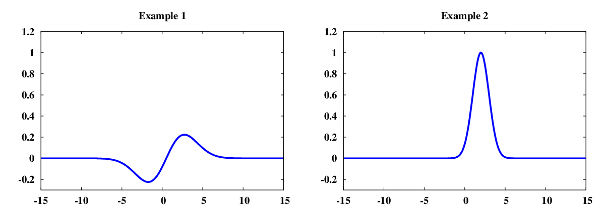
Refer to caption
Figure 1. Initial data used in the first experiment, in relation to the accuracy order.

As it can be observed in Figure 2, the slopes for the numerical solutions at T=10T=10 corresponding to those initial data are consistent with the theoretical results of Section 2. A line of slope one has been added as a reference for the convergence order.

Refer to caption
Figure 2. Accuracy order for the initial data shown in Figure 1 using several time-step sizes. The plot shows ‖u1​(10)−u2​(10)‖L2​(ℝ)\|u_{1}(10)-u_{2}(10)\|_{L^{2}(\mathbb{R})}, where u1u_{1} and u2u_{2} have been computed using Δ​t{\Delta t} and Δ​t/2{\Delta t}/2 respectively.

Furthermore, we also show the convergence rate of the numerical solutions towards the asymptotic profile of the augmented Burgers equation, given in Theorem 1.2. Let us remark that uMu_{M} is now the asymptotic profile of the viscous Burgers equation with 1/Γ+cν1/\Gamma+c_{\nu} viscosity coefficient instead of 22 (see [11] for the complete expression for uMu_{M}). We compare the splitting method described above with the discretization proposed in [11], where a rectangle method is used to approximate the convolution in (1.1). In Figure 3 we plot the solution at time T=12000T=12000 for the given initial data, as well as the corresponding asymptotic profile uMu_{M}. Then, in Figure 4 we can observe that the convergence rates meet the ones defined in (1.9), preserving the large-time behavior of the solution of equation (1.1).
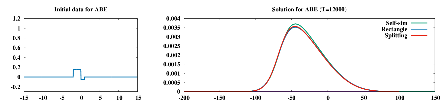
Refer to caption
Figure 3. Initial data and solution for ABE with Γ=100\Gamma=100 and cν=0.02c_{\nu}=0.02 at T=12000T=12000. We compare the splitting method (blue) with the one from [11] discretized explicitly in time (red). The self-similar asymptotic profile (green) is given as reference too.
Refer to caption
Figure 4. Evolution of the L1L^{1} and L2L^{2} norms of the difference between the asymptotic profile and the solution, multiplied by their corresponding rate, as in (1.9). We compare the splitting method (blue) and the one from [11] discretized explicitly in time (red).

Aknowledgements

L. I. Ignat was partially supported by a grant of the Romanian National Authority for Scientific Research and Innovation, CNCS-UEFISCDI, project number PN-II-RU-TE-2014-4-0007, Grant MTM2014-52347, MICINN, Spain and FA9550-15-1-0027 of AFOSR. A. Pozo was granted by the Basque Government, reference PRE_2013_2_150, and partially supported by ERCEA under Grant 246775 NUMERIWAVES, by the Basque Government through the BERC 2014-2017 program and by Spanish MINECO: BCAM Severo Ochoa excellence accreditation SEV-2013-0323.

References

  • [1] J. Aguirre, M. Escobedo, and E. Zuazua, Self-similar solutions of a convection diffusion equation and related semilinear elliptic problems, Communications in Partial Differential Equations 15 (1990), no. 2, 139–157.
  • [2] Juan J. Alonso and Michael R. Colonno, Multidisciplinary optimization with applications to sonic-boom minimization, Annual Review of Fluid Mechanics 44 (2012), 505–526.
  • [3] Afaf Bouharguane and Rémi Carles, Splitting methods for the nonlocal fowler equation, Mathematics of Computation 83 (2013), 1221–1141.
  • [4] Carlos Castro, Francisco Palacios, and Enrique Zuazua, Optimal control and vanishing viscosity for the Burgers equation, Integral Methods in Science and Engineering (C. Costanda and M. E. Pérez, eds.), vol. 2, Birkhäuser Verlag, 2010, pp. 65–90.
  • [5] Robin Olev Cleveland, Propagation of sonic booms through a real, stratified atmosphere, Ph.D. thesis, University of Texas at Austin, 1995.
  • [6] Michael G. Crandall and Andrew Majda, The method of fractional steps for conservation laws, Numerische Mathematik 34 (1980), 285–314.
  • [7] Miguel Escobedo and Enrique Zuazua, Large time behavior for convection-diffusion equations in ℝn\mathbb{R}^{n}, Journal of Functional Analysis 100 (1991), no. 1, 119–161.
  • [8] Helge Holden, Kenneth H. Karlsen, Knut-Andreas Lie, and Nils Henrik Risebro, Splitting methods for partial differential equations with rough solutions, EMS Series of Lectures in Mathematics, European Mathematical Society, 2010.
  • [9] Helge Holden, Christian Lubich, and Nils Henrik Risebro, Operator splitting for partial differential equations with burgers nonlinearity, Mathematics of Computation 82 (2013), no. 281, 173–185.
  • [10] Liviu I. Ignat, Tatiana I. Ignat, and Denisa Stancu-Dumitru, A compactness tool for the analysis of nonlocal evolution equations, SIAM Journal on Mathematical Analysis 47 (2015), no. 2, 1330–1354.
  • [11] Liviu I. Ignat and Alejandro Pozo, A semi-discrete large-time behavior preserving scheme for the augmented Burgers equation, https://arxiv.org/abs/1409.3817.
  • [12] Liviu I. Ignat, Alejandro Pozo, and Enrique Zuazua, Large-time asymptotics, vanishing viscosity and numerics for 1-d scalar conservation laws, Mathematics of Computation 84 (2015), 1633–1662.
  • [13] Liviu I. Ignat and Julio D. Rossi, A nonlocal convection-diffusion equation, Journal of Functional Analysis 251 (2007), 399–437.
  • [14] by same author, Decay estimates for nonlocal problems via energy methods, Journal de Mathématiques Pures et Appliquées 92 (2009), no. 2, 163–187.
  • [15] Arieh Iserles, A first course in the numerical analysis of differential equations, Cambridge University Press, 1996.
  • [16] Sriram K. Rallabhandi, Advanced sonic boom prediction using augmented Burger’s equation, Journal of Aircraft 48 (2011), no. 4, 1245–1253.
  • [17] by same author, Sonic boom adjoint methodology and its applications, 29th AIAA Applied Aerodynamics Conference, American Institute of Aeronautics and Astronautics, June 2011.