Efficient and Qualified Mesh Generation for Gaussian Molecular Surface Using Piecewise Trilinear Polynomial Approximation

Tiantian Liu ^†^†thanks: State Key Laboratory of Scientific and Engineering Computing, Institute of Computational Mathematics and Scientific Engineering Computing, Academy of Mathematics and Systems Science, Chinese Academy of Sciences, Beijing 100190, China. Corresponding author: Benzhuo Lu (E-mail: bzlu@lsec.cc.ac.cn). Minxin Chen ^†^†thanks: Center for System Biology, Department of Mathematics, Soochow University, Suzhou 215006, China. Corresponding author: Minxin Chen (E-mail: chenminxin@suda.edu.cn). Benzhuo Lu^*

Abstract

Recent developments for mathematical modeling and numerical simulation of biomolecular systems raise new demands for qualified, stable, and efficient surface meshing, especially in implicit-solvent modeling¹. In our former work, we have developed an algorithm for manifold triangular meshing for large Gaussian molecular surfaces, TMSmesh^{2, 3}. In this paper, we present new algorithms to greatly improve the meshing efficiency and qualities, and implement into a new program version, TMSmesh 2.0. In TMSmesh 2.0, in the first step, a new adaptive partition and estimation algorithm is proposed to locate the cubes in which the surface are approximated by piecewise trilinear surface with controllable precision. Then, the piecewise trilinear surface is divided into single valued pieces by tracing along the fold curves, which ensures that the generated surface meshes are manifolds. Numerical test results show that TMSmesh 2.0 is capable of handling arbitrary sizes of molecules and achieves ten to hundreds of times speedup over the previous algorithm. The result surface meshes are manifolds and can be directly used in boundary element method (BEM) and finite element method (FEM) simulation. The binary version of TMSmesh 2.0 is downloadable at the web page http://lsec.cc.ac.cn/ $\sim$ lubz/Meshing.html.

Keywords: surface mesh generation; Gaussian surface; triangulation; adaptive partition; trilinear polynomial

1 Introduction

Molecular surface mesh generation is a prerequisite for using boundary element method (BEM) and finite element method (FEM) in the implicit-solvent modeling (e.g., see a review in ¹). Recent developments in implicit-solvent modeling of biomolecular systems raise new demands for qualified, stable, and efficient surface meshing. Main concerns for improvement on existing methods for molecular surface mesh generation are efficiency, robustness, and mesh quality. Efficiency is necessary for simulations/computations requiring frequent mesh generation or requiring meshing for large systems. Robustness here means the meshing method is stable and can treat various, even arbitrary, sizes of molecular systems within computer power limitations. Mesh quality relates to mesh smoothness (avoiding sharp solid angles, etc.), uniformness (avoiding elements with very sharp angles or zero area), topological correctness (manifoldness, avoiding isolated vertices, element intersection, single-element-connected edges, etc.) and fidelity (faithful to the original defined molecular surface). The quality requirement is critical for some numerical techniques, such as finite element method, to achieve converged and reasonable results, which makes it a more demanding task in this aspect than the mesh generations only for the purposes of visualization or some structural geometry analysis.

There are various kinds of definitions for molecular surface, including the van der Waals (VDW) surface, the solvent accessible surface (SAS)⁴, the solvent excluded surface (SES)⁵, the minimal molecular surface⁶, the molecular skin surface⁷ and the Gaussian surface. The VDW surface is defined as the surface of the union of the spherical atomic surfaces with VDW radius of each atom within the molecule. The SAS and SES are represented by the trajectory of the center and the inter-boundary of a rolling probe on the VDW surface, respectively. The minimal molecular surface is defined as the result of the minimization of a type of surface energy. The molecular skin surface is the envelope of an infinite family of spheres derived from atoms by convex combination and shrinking. The Gaussian surface is defined as a level set of the summation of Gaussian kernel functions:

\{\vec{x}\in R^{3},\phi\left(\vec{x}\right)=c\},

(1)

where

\phi\left(\vec{x}\right)=\sum_{i=1}^{N}e^{-D(\|\vec{x}-\vec{x}_{i}\|^{2}-r_{i}^{2})},

(2)

$\vec{x}_{i}$ and $r_{i}$ are the location and radius of the $i$ th atom. $D$ is the decay rate of the Gaussian kernel. $c$ is the isovalue and it controls the volume enclosed by the Gaussian surface. These two parameters, $D$ and $c$ can be chosen properly to make the Gaussian surface approximate the SES, SAS and VDW surface well.⁸

For SAS and SES, numerous works have been committed to the computation of the molecular surface in the literature. In 1983, Connolly proposed algorithms to calculate the molecular surface and SAS analytically.^{9, 10} In 1995, a popular program, GRASP, for visualizing molecular surfaces was presented.¹¹ An algorithm named SMART for triangulating SAS into curvilinear elements was proposed by Zauhar¹². The software MSMS was proposed by Sanner et al. in 1996 to mesh the SES and is a widely used program for molecular surface triangulation due to its high efficiency.¹³ In 1997, Vorobjev et al. proposed SIMS, a method of calculating a smooth invariant molecular dot surface, in which an exact method for removing self-intersecting parts and smoothing the singular regions of the SES was presented.¹⁴ Ryu et al. proposed a method based on beta-shapes¹⁵, which is a generalization of alpha shapes¹⁶. Can et al. proposed LSMS to generate the SES on grid points using level-set methods.¹⁷ In 2009, a program, EDTsurf, based on LSMS was proposed used for generating the VDW surface, SES and SAS.¹⁸ A ray-casting-based algorithm, NanoShaper, is proposed to generate SES, skin surface and Gaussian surface in 2013.¹⁹

For skin surface, Chavent et al. presented MetaMtal to visualize the molecular skin surface using ray-casting method ²⁰, and Cheng et al. used restricted union of balls to generate mesh for molecular skin surface²¹. For minimal surface, Wei et al. ⁶ constructed a surface-based energy functional, and use minimization and isosurface extraction processes to obtain a so-called minimal molecular surface.

For the Gaussian surface, existing techniques for triangulating an implicit surface can be used to mesh the Gaussian surface. These methods are divided into two main categories: spatial partition and continuation methods. The well known marching cube method ²² and dual contouring method ²³ are examples of the spatial partition methods. In 2006, Zhang et al. ²⁴ used a modified dual contouring method to generate meshes for biomolecular structures. A later tool, GAMer ²⁵, was developed for both the generation and improvement of the Gaussian surface meshes. An efficient mesh generation algorithm accelerated by multi-core CPU and GPU was also proposed in 2013.²⁶

Most of those software have some issues according to above mentioned criteria for mesh generation, e.g., MSMS and GAMer generate many non-manifold defects in the mesh, fidelity is not well preserved for the EDTsurf and GAMer surfaces, and for the marching cube and grid-based methods the memory requirements can be huge when treating large molecules. More detailed comparison and discussion of the software can be found in ⁸. As MSMS is a most commonly used software in this area, we will still use it as a main reference for our new algorithm in this article. In 2011, we have proposed an algorithm and implemented in the program TMSmesh for triangular meshing of the Gaussian surface.^{2, 3, 8} The trace technique which is a generalization of adaptive predictor-corrector technique is used in TMSmesh to connect sampled surface points. TMSmesh contains two steps. The first step is to compute the intersection points between the molecular Gaussian surface and the lines parallel to $x$ -axis. In the second step, the sampled surface points are connected through three algorithms to form loops, and the whole closed manifold surface is decomposed into a collection of patches enclosed by loops on the surface. The patches are finally single valued on $x,y,z$ directions, so these pieces can be treated as 2-dimensional polygons and be easily triangulated through standard triangulation algorithms. In TMSmesh, there are no problems of overlapping, gap filling, and selecting seeds that need to be considered in traditional continuation methods. TMSmesh performs well in the following aspects. Firstly, TMSmesh is robust. TMSmesh succeeds to generate surface meshes for biomolecules comprised of more than one million atoms. Secondly, the meshes produced by TMSmesh have good qualities (uniformness, manifoldness). Thirdly, the generated surface mesh preserves the original molecular surface features and properties (topology, surface area and enclosed volume, and local curvature). However, as to the aspect of computational efficiency, although the computational complexity is linear with respect to the number of atoms as shown in ³, the overall low efficiency of TMSmesh still needs to be improved.

In this paper, we proposed a new algorithm and updated program version TMSmesh 2.0 to mesh the Gaussian surface efficiently. Firstly, the space are adaptively divided into cubes and an algorithm of dividing cubes and estimating the error between the Gaussian surface and approximated trilinear polynomial in each cube is developed. With this algorithm, the Gaussian surface is approximated by piecewise trilinear surface. Then, in each cube, the trilinear surface is divided into a collection of single valued pieces on $x,y,z$ directions by tracing along fold curves (in the trilinear surface case the fold curve can be directly calculated analytically). Finally, each single valued piece is triangulated by ear clipping algorithm^{27, 28}.

This paper is organized as follows. The new algorithm for triangulating the Gaussian surface is introduced in the Meshing Algorithm Section. In the Experimental Results Section, some examples and applications are presented. The final section, Conclusion, gives some concluding remarks.

2 Meshing Algorithm

2.1 Algorithm Outline

In this section, we describe the algorithms to construct the triangular surface meshes. The inputs of our method are PQR files which contains a list of centers and radii of atoms. The output of our method are OFF files which contains the triangular meshes. Our algorithm contains two stages, the first stage is an adaptive estimation and division process. The Gaussian surface is approximated by piecewise trilinear surface within controllable error. The second stage is to partition each piece of trilinear surface into single valued patches along $x,y,z$ directions by tracing along the fold curves. Then each single valued patch is triangulated by the ear clipping algorithm^{27, 28}. In the following subsections, each stage is described in detail.

2.2 Approximating the Gaussian Surface by Piecewise Trilinear Surface

In this stage, the space is divided into cubes adaptively and in each final cube, the Gaussian surface is close to a trilinear surface whose error is controllable. Initially, the molecule is placed in a three-dimensional orthogonal grid consisting $n_{x}\times n_{y}\times n_{z}$ cubes. The initial grid is very coarse. Then the grid is refined adaptively by the following estimation and division steps.

•

Step 1, In each cube, $\phi(x,y,z)$ is approximated by a nth-degree polynomial $\tilde{P}(x,y,z)$ , i.e., the Gaussian surface $\phi(x,y,z)=c$ is replaced by the polynomial surface $\tilde{P}(x,y,z)=c$ .
•

Step 2, the lower and the upper bound of $\tilde{P}(x,y,z)$ , denoted by $L$ and $U$ , in each cube is estimated. If the isovalue $c$ belongs to $[L,U]$ , the cube has intersection with the surface $\tilde{P}(x,y,z)=c$ and we go to Step 3, otherwise, the cube is abandoned.
•

Step 3, divide each left cube into 8 smaller child cubes, and compute the expression of $\tilde{P}(x,y,z)$ in each child cube. When the child cubes become smaller, the coefficients of higher order terms (higher than the linear order) of $\tilde{P}(x,y,z)$ go to zero. If they are under some user-specified bound, approximate $\tilde{P}(x,y,z)$ by trilinear polynomial, otherwise, go to Step 2.

With above processes, the Gaussian surface finally is approximated by piecewise trilinear surfaces in cubes with different sizes. In the following subsections, we explain the details of above estimation and division process.

2.2.1 Approximation with nth-degree polynomial

Firstly, without loss of generality, we only consider the case of $D=1$ , then eq (2) is written into the following one:

\phi\left(\vec{x}\right)=\sum_{i=1}^{N}e^{-(\|\vec{x}-\vec{x}_{i}\|^{2}-r_{i}^{2})}=\sum_{i=1}^{N}e^{r_{i}^{2}}e^{-\left(x-x_{i}\right)^{2}}e^{-\left(y-y_{i}\right)^{2}}e^{-\left(z-z_{i}\right)^{2}}.

(3)

In an arbitrary cube $[a,b]\times[c,d]\times[e,f]$ , eq (3) can be approximated by

P(x,y,z)=\sum_{i=1}^{N}e^{r_{i}^{2}}P_{n}(x,x_{i},a,b)Q_{n}(y,y_{i},c,d)R_{n}(z,z_{i},e,f),

(4)

where

P_{n}(x,x_{i},a,b)=\sum_{j=0}^{n}\alpha_{j}(x_{i},a,b)L_{j}(\frac{2x-(a+b)}{b-a}),

(5)

Q_{n}(y,y_{i},a,b)=\sum_{j=0}^{n}\beta_{j}(y_{i},c,d)L_{j}(\frac{2y-(c+d)}{d-c}),

(6)

R_{n}(z,z_{i},e,f)=\sum_{j=0}^{n}\gamma_{j}(z_{i},e,f)L_{j}(\frac{2z-(e+f)}{f-e}),

(7)

and

\alpha_{j}=\frac{2}{b-a}\int_{a}^{b}\phi(\frac{2x-(a+b)}{b-a})L_{j}(\frac{2x-(a+b)}{b-a})\,dx,

\beta_{j}=\frac{2}{d-c}\int_{c}^{d}\phi(\frac{2y-(c+d)}{d-c})L_{j}(\frac{2y-(c+d)}{d-c})\,dy,

\gamma_{j}=\frac{2}{f-e}\int_{e}^{f}\phi(\frac{2z-(e+f)}{f-e})L_{j}(\frac{2z-(e+f)}{f-e})\,dz,

$L_{j}(\cdot)$ is Legendre polynomial of order $j$ and n is set as 3 in our work. However, $P(x,y,z)$ is not continuous between neighbored cubes, so we do the following corrections of $P(x,y,z)$ to make $P(x,y,z)$ be $C^{0}$ continuous in the whole domain. For one component $P_{n}(x,x_{i},a,b)$ , we introduce two variables $\epsilon_{0}(x_{i},a,b)$ and $\epsilon_{1}(x_{i},a,b)$ as follows.

$\displaystyle\tilde{P}_{n}(x,x_{i},a,b)$	$\displaystyle=P_{n}(x,x_{i},a,b)+\epsilon_{0}(x_{i},a,b)L_{n-1}(\frac{2x-(a+b)}{b-a})+\epsilon_{1}(x_{i},a,b)L_{n}(\frac{2x-(a+b)}{b-a})$	(8)
	$\displaystyle=\alpha_{0}(x_{i},a,b)L_{0}(\frac{2x-(a+b)}{b-a})+\cdots+\alpha_{n}(x_{i},a,b)L_{n}(\frac{2x-(a+b)}{b-a})$
	$\displaystyle+\epsilon_{0}(x_{i},a,b)L_{n-1}(\frac{2x-(a+b)}{b-a})+\epsilon_{1}(x_{i},a,b)L_{n}(\frac{2x-(a+b)}{b-a}).$

The following two equations make $\tilde{P}_{n}(x,x_{i},a,b)$ equal $x$ component of $\phi\left(\vec{x}\right)$ on the boundary of the box and be $C^{0}$ continuous along $x$ directions.


		$\displaystyle\tilde{P}_{n}(a,x_{i},a,b)=e^{-(a-x_{i})^{2}}$			(9a)
		$\displaystyle\tilde{P}_{n}(b,x_{i},a,b)=e^{-(b-x_{i})^{2}}.$			(9b)

$\epsilon_{0}(x_{i},a,b)$ and $\epsilon_{1}(x_{i},a,b)$ can be easily solved from eq (9). Then $\tilde{P}_{n}(x,x_{i},a,b)$ is written as the following one:

\tilde{P}_{n}(x,x_{i},a,b)=\sum_{j=0}^{n}\tilde{\alpha}_{j}(x_{i},a,b)L_{j}(\frac{2x-(a+b)}{b-a}),

(10)

where

\tilde{\alpha}_{j}(x_{i},a,b)=\begin{cases}\alpha_{j}(x_{i},a,b)&\text{$j<n-1$},\\ \alpha_{n-1}(x_{i},a,b)+\epsilon_{0}(x_{i},a,b)&\text{$j=n-1$},\\ \alpha_{n}(x_{i},a,b)+\epsilon_{1}(x_{i},a,b)&\text{$j=n$}.\end{cases}

(11)

After above correction, $\tilde{P}_{n}(x,x_{i},a,b)$ is the best least square approximation for $x$ component of $\phi(\vec{x})$ in the space spanned by { $L_{i}$ , $i=0,...,n-2$ } and it is also $C^{0}$ continuous on the boundaries of the cubes along $x$ direction. The same method should be used to correct $Q_{n}(y,y_{i},c,d)$ and $R_{n}(z,z_{i},e,f)$ to make $\tilde{P}(x,y,z)$ be $C^{0}$ continuous along $y,z$ directions. We have

\tilde{Q}_{n}(y,y_{i},a,b)=\sum_{j=0}^{n}\tilde{\beta}_{j}(y_{i},c,d)L_{j}(\frac{2y-(c+d)}{d-c}),

(12)

\tilde{R}_{n}(z,z_{i},e,f)=\sum_{j=0}^{n}\tilde{\gamma}_{j}(z_{i},e,f)L_{j}(\frac{2z-(e+f)}{f-e}),

(13)

where the forms of $\tilde{\beta}_{j}(y_{i},c,d)$ and $\tilde{\gamma}_{j}(z_{i},e,f)$ are similar to $\tilde{\alpha}_{j}(x_{i},a,b)$ in eq (11). Then the new $n$ -th polynomial is written as

\tilde{P}(x,y,z)=\sum_{i=1}^{N}e^{r_{i}^{2}}\tilde{P}_{n}(x,x_{i},a,b)\tilde{Q}_{n}(y,y_{i},c,d)\tilde{R}_{n}(z,z_{i},e,f)

(14)

for $x\in[a,b],y\in[c,d],z\in[e,f]$ . In practical computation of $\tilde{P}(x,y,z)$ , we only need to compute the summation in eq (14) with respect to the neighborhood $\{x_{i},y_{i},z_{i}\}$ of the cube $[a,b]*[c,d]*[e,f]$ , since the kernel $e^{-||\vec{x}-\vec{x}_{i}||^{2}}$ decay very quickly when $||\vec{x}-\vec{x}_{i}||$ goes to large.

2.2.2 Estimation of upper and lower bound of $\tilde{P}(x,y,z)$

In order to rule out the cubes having no surface points, the lower and upper bound of $\tilde{P}(x,y,z)$ in the cube is estimated. $\tilde{P}(x,y,z)$ in eq (14) can be written in the form of product of tensor:

\tilde{P}(x,y,z)=A\bar{\times}_{1}\vec{L}(\frac{2x-(a+b)}{b-a})\bar{\times}_{2}\vec{L}(\frac{2y-(c+d)}{d-c})\bar{\times}_{3}\vec{L}(\frac{2z-(e+f)}{f-e}),

(15)

where $A=\sum_{i=1}^{N}e^{r_{i}^{2}}B_{i}$ and


		$\displaystyle B_{i}=b_{i}^{(1)}\otimes b_{i}^{(2)}\otimes b_{i}^{(3)}$			(16a)
		$\displaystyle b_{i}^{(1)}=(\tilde{\alpha}_{0}(x,x_{i},a,b),\tilde{\alpha}_{1}(x,x_{i},a,b),\cdots,\tilde{\alpha}_{n}(x,x_{i},a,b))$			(16b)
		$\displaystyle b_{i}^{(2)}=(\tilde{\beta}_{0}(y,y_{i},a,b),\tilde{\beta}_{1}(y,y_{i},a,b),\cdots,\tilde{\beta}_{n}(y,y_{i},a,b))$			(16c)
		$\displaystyle b_{i}^{(3)}=(\tilde{\gamma}_{0}(z,z_{i},a,b),\tilde{\gamma}_{1}(z,z_{i},a,b),\cdots,\tilde{\gamma}_{n}(z,z_{i},a,b))$			(16d)
		$\displaystyle\vec{L}(\frac{2x-(a+b)}{b-a})=(L_{0}(\frac{2x-(a+b)}{b-a}),\cdots,L_{n}(\frac{2x-(a+b)}{b-a}))$			(16e)
		$\displaystyle\vec{L}(\frac{2y-(c+d)}{d-c})=(L_{0}(\frac{2y-(c+d)}{d-c}),\cdots,L_{n}(\frac{2y-(c+d)}{d-c}))$			(16f)
		$\displaystyle\vec{L}(\frac{2z-(e+f)}{f-e})=(L_{0}(\frac{2z-(e+f)}{f-e}),\cdots,L_{n}(\frac{2z-(e+f)}{f-e})).$			(16g)

$\otimes$ is the product of tensor. $\bar{\times}_{k}$ is $k$ -mode (vector) product of a tensor $X\in\mathbb{R}^{I_{1}\times I_{2}\times I_{3}}$ with a vector $V\in\mathbb{R}^{I_{k}}$ denoted by $X\bar{\times}_{k}V$ and is of size $I_{1}\times\cdots\times I_{k-1}\times I_{k+1}\times\cdots\times I_{3}$ . ²⁹ Its $i_{1}\cdots i_{k-1}i_{k+1}\cdots i_{3}$ entry is as follows.

(X\bar{\times}_{k}V)_{i_{1}\cdots i_{k-1}i_{k+1}\cdots i_{3}}=\sum_{i_{k}=1}^{I_{k}}x_{i_{1}}x_{i_{2}}x_{i_{3}}v_{i_{k}}.

(17)

$A$ is a three-dimensional tensor whose size is $(n+1)\times(n+1)\times(n+1)$ , where $n$ is the degree of the polynomial $\tilde{P}(x,y,z)$ . To get the lower and upper bound of $\tilde{P}(x,y,z)$ , firstly, the main part of $\tilde{P}(x,y,z)$ is obtained by doing singular value decomposition (SVD) for $A$ . Secondly, the upper and the lower bounds of the main part and the remainder are estimated respectively.

Here we use Singular Value Decomposition(SVD) for $A$ to approximate $\tilde{P}(x,y,z)$ by a multiplication of three polynomials in $x,y,z,$ respectively. Taking $n=3$ and $A=[a_{ij}]_{4\times 4\times 4}$ for example, the algorithm of SVD is as follows.

Step 1, transform A into a two-dimensional matrix.

A_{1}=\begin{bmatrix}a_{111}&\dots&a_{141}&a_{211}&\dots&a_{241}&a_{311}&\dots&a_{341}&a_{411}&\dots&a_{441}\\ a_{112}&\dots&a_{142}&a_{212}&\dots&a_{242}&a_{312}&\dots&a_{342}&a_{412}&\dots&a_{442}\\ a_{113}&\dots&a_{143}&a_{213}&\dots&a_{243}&a_{313}&\dots&a_{343}&a_{413}&\dots&a_{443}\\ a_{114}&\dots&a_{144}&a_{214}&\dots&a_{244}&a_{314}&\dots&a_{344}&a_{414}&\dots&a_{444}\end{bmatrix}

(18)

Step 2, do singular value decomposition to $A_{1}$ .

A_{1}=UDV^{\ast},

(19)

where $U=(\vec{u}_{1},\vec{u}_{2},\vec{u}_{3},\vec{u}_{4})$ is a $4\times 4$ matrix, $V^{\ast}$ is a $4\times 16$ matrix and

D=\begin{bmatrix}\sigma_{1}&0&0&0\\ 0&\sigma_{2}&0&0\\ 0&0&\sigma_{3}&0\\ 0&0&0&\sigma_{4}\end{bmatrix}

(20)

If $j$ satisfies

\text{min}\{j:\sum_{i=1}^{j}\sigma_{i}\geq 0.99\sum_{i=1}^{4}\sigma_{i}\},

(21)

we reserve $\sigma_{1},\dots,\sigma_{j}$ and abandon $\sigma_{j+1},\dots,\sigma_{4}$ .

Step 3, transform each row of $V^{\ast}$ into a square matrix. If

V^{\ast}=\begin{bmatrix}v_{1,1}&v_{1,2}&\dots&v_{1,16}\\ v_{2,1}&v_{2,2}&\dots&v_{2,16}\\ v_{3,1}&v_{3,2}&\dots&v_{3,16}\\ v_{4,1}&v_{4,2}&\dots&v_{4,16}\end{bmatrix},

(22)

we can transform the $i$ -th row of $V^{\ast}$ into a $4\times 4$ matrix denoted by $V_{i}$ :

V_{i}=\begin{bmatrix}v_{i,1}&v_{i,2}&v_{i,3}&v_{i,4}\\ v_{i,5}&v_{i,6}&v_{i,7}&v_{i,8}\\ v_{i,9}&v_{i,10}&v_{i,11}&v_{i,12}\\ v_{i,13}&v_{i,14}&v_{i,15}&v_{i,16}\end{bmatrix}.

(23)

Step 4, do SVD for $V_{i}$ respectively.

V_{i}=W_{i}D_{i}Z_{i},

(24)

where $W_{i}=(\vec{w_{1}^{i}},\vec{w_{2}^{i}},\vec{w_{3}^{i}},\vec{w_{4}^{i}}),D_{i}=diag(d_{1}^{i},d_{2}^{i},d_{3}^{i},d_{4}^{i}),Z_{i}=(\vec{z_{1}^{i}},\vec{z_{2}^{i}},\vec{z_{3}^{i}},\vec{z_{4}^{i}})^{T}$ . If $j_{i}$ satisfies

\text{min}\{j_{i}:\sum_{k=1}^{j_{i}}d_{k}^{i}\geq 0.99\sum_{k=1}^{4}d_{k}^{i}\},

$d_{1}^{i},\dots,d_{j_{i}}^{i}$ are reserved and $d_{j_{i}+1}^{i},\dots,d_{4}^{i}$ are abandoned. Therefore, $V_{i}$ can be approximated by the following formula

V_{i}\approx d_{1}^{i}\vec{w_{1}^{i}}\otimes\vec{z_{1}^{i}}+\dots+d_{j_{i}}^{i}\vec{w_{j_{1}}^{i}}\otimes\vec{z_{j_{i}}^{i}}.

(25)

Through the above calculation, $A$ can be approximated by

A\approx\sum_{i=1}^{j}\sigma_{i}\vec{u}_{i}\otimes(\sum_{k=1}^{j_{i}}d_{i}^{k}\vec{w_{i}^{k}}\otimes\vec{z_{i}^{k}}).

(26)

The summation at the right side of eq (26) is denoted by $\tilde{A}$ . As a result, $A$ can be split by $A=\tilde{A}+R$ , where $\tilde{A}$ is the main part and $R$ is the residue part.

With above SVD process, $\tilde{P}(x,y,z)$ can be converted to the following form:

\tilde{P}(x,y,z)=S(x,y,z)+T(x,y,z),\\

(27)

where

S(x,y,z)=\tilde{A}\times_{1}\vec{L}(\frac{2x-(a+b)}{b-a})\times_{2}\vec{L}(\frac{2y-(c+d)}{d-c})\times_{3}\vec{L}(\frac{2z-(e+f)}{f-e}),

(28)

T(x,y,z)=R\times_{1}\vec{L}(\frac{2x-(a+b)}{b-a})\times_{2}\vec{L}(\frac{2y-(c+d)}{d-c})\times_{3}\vec{L}(\frac{2z-(e+f)}{f-e}).

(29)

For $S(x,y,z)$ , the upper bound and lower bound are estimated through the following steps.

S(x,y,z)=\sum_{i=1}^{j}\sigma_{i}\tilde{U}^{i}(x)\left[\sum_{k=1}^{j_{i}}d_{k}^{i}\tilde{W}_{k}^{i}(y)\tilde{Z}_{k}^{i}(z)\right],

(30)

where


		$\displaystyle\tilde{U}^{i}(x)=\vec{u}_{i}\cdot\vec{L}(\frac{2x-(a+b)}{b-a})$			(31a)
		$\displaystyle\tilde{W}_{k}^{i}(y)=\vec{w_{k}^{i}}\cdot\vec{L}(\frac{2y-(c+d)}{d-c})$			(31b)
		$\displaystyle\tilde{Z}_{k}^{i}(z)=\vec{z_{k}^{i}}\cdot\vec{L}(\frac{2z-(e+f)}{f-e}).$			(31c)

Firstly, we estimate the upper bound and lower bound of one dimensional polynomial $\tilde{W}_{k}^{i}(y)$ and $\tilde{Z}_{k}^{i}(z)$ respectively. The upper and lower bound of $\tilde{W}_{k}^{i}(y)$ are denoted by $M_{k}^{y}$ and $m_{k}^{y}$ . And the upper and lower bound of $\tilde{Z}_{k}^{i}(z)$ are denoted by $M_{k}^{z}$ and $m_{k}^{z}$ . Secondly, the upper bound and lower bound of $\tilde{W}_{k}^{i}(y)\tilde{Z}_{k}^{i}(z)$ are estimated by

M_{k}^{yz}=max\{M_{k}^{y}M_{k}^{z},M_{k}^{y}m_{k}^{z},m_{k}^{y}M_{k}^{z},m_{k}^{y}m_{k}^{z}\},

(32)

m_{k}^{yz}=min\{M_{k}^{y}M_{k}^{z},M_{k}^{y}m_{k}^{z},m_{k}^{y}M_{k}^{z},m_{k}^{y}m_{k}^{z}\}.

(33)

Then the upper bound of $\sum_{k=1}^{j_{i}}d_{k}^{i}\tilde{W}_{k}^{i}(y)\tilde{Z}_{k}^{i}(z)$ is

M_{i}^{yz}=\sum_{k=1}^{j_{i}}d_{k}^{i}M_{k}^{yz}

(34)

and the lower bound is

m_{i}^{yz}=\sum_{k=1}^{j_{i}}d_{k}^{i}m_{k}^{yz}.

(35)

Finally, we estimate the upper bound and the lower bound of $\tilde{U}^{i}(x)$ which are denoted by $M_{i}^{x}$ and $m_{i}^{x}$ . Then the bounds of $\tilde{U}^{i}(x)\left[\sum_{k=1}^{j_{i}}d_{k}^{i}\tilde{W}_{k}^{i}(y)\tilde{Z}_{k}^{i}(z)\right]$ can be estimated by

M_{i}=max\{M_{i}^{x}M_{i}^{yz},M_{i}^{x}m_{i}^{yz},m_{i}^{x}M_{i}^{yz},m_{i}^{x}m_{i}^{yz}\},

(36)

m_{i}=min\{M_{i}^{x}M_{i}^{yz},M_{i}^{x}m_{i}^{yz},m_{i}^{x}M_{i}^{yz},m_{i}^{x}m_{i}^{yz}\}.

(37)

Therefore, the upper bound and lower bound of $S(x,y,z)$ is

M=\sum_{i=1}^{j}\sigma_{i}M_{i}

(38)

and

m=\sum_{i=1}^{j}\sigma_{i}m_{i}.

(39)

The range of each entry of $\vec{L}(\cdot)$ is $[-1,1]$ . Therefore, $T(x,y,z)$ can be estimated by

$\displaystyle\|T(x,y,z)\|$	$\displaystyle=\|R\times_{1}\vec{L}(\frac{2x-(a+b)}{b-a})\times_{2}\vec{L}(\frac{2y-(c+d)}{d-c})\times_{3}\vec{L}(\frac{2z-(e+f)}{f-e})\|$	(40)
	$\displaystyle\leq\|\sum R_{ijk}\|$
	$\displaystyle\leq\sum\|R_{ijk}\|,$

where $R_{ijk}$ is the $(i,j,k)$ entry of $R$ .

As a result, the upper and lower bound of $\tilde{P}(x,y,z)$ is

U=M+\sum|R_{ijk}|,

(41)

L=m-\sum|R_{ijk}|.

(42)

If the bounds satisfy the condition that $L\leq c\leq U$ , the surface may have intersection with the cube. Otherwise, the cube should be ruled out.

2.2.3 Approximation by trilinear polynomial

In each left cube, $\phi(x,y,z)$ is approximated by polynomial $\tilde{P}(x,y,z)$ as shown in eq (15). Then we divide each left cube into 8 smaller child cubes, and express $\tilde{P}(x,y,z)$ in each child cube by Legendre polynomials as follows

\tilde{P}(x,y,z)=A^{\prime}\times_{1}\vec{L}(\frac{2x-(a+b)}{b-a})\times_{2}\vec{L}(\frac{2y-(c+d)}{d-c})\times_{3}\vec{L}(\frac{2z-(e+f)}{f-e}),

(43)

where $x\in[a_{1},b_{1}],y\in[c_{1},d_{1}]$ and $z\in[e_{1},f_{1}]$ . Here, $[a_{1},b_{1}]\times[c_{1},d_{1}]\times[e_{1},f_{1}]$ is the range of the child cube and $A^{\prime}$ is the coefficient tensor of the Legendre polynomials in the child cube. When the child cubes become smaller, the coefficients of the higher order Legendre polynomials in the coefficient tensor go to zero. The division process is repeated until the coefficients of the higher order Legendre polynomials are close to zero enough to be neglected in all the left cubes.

After above division and estimation process, in each left cube, we approximate the surface $\tilde{P}(x,y,z)=c$ by the following trilinear interpolation. Supposing the range of the left cube is $[-1,1]\times[-1,1]\times[-1,1]$ , the trilinear interpolation can be written in terms of the vertex values:

$\displaystyle g(x,y,z)=$	$\displaystyle\frac{1}{8}[\tilde{P}(-1,-1,-1)(1-x)(1-y)(1-z)+\tilde{P}(-1,-1,1)(1-x)(1-y)(1+z)$	(44)
	$\displaystyle+\tilde{P}(-1,1,-1)(1-x)(1+y)(1-z)+\tilde{P}(-1,1,1)(1-x)(1+y)(1+z)$
	$\displaystyle+\tilde{P}(1,-1,-1)(1+x)(1-y)(1-z)+\tilde{P}(1,-1,1)(1+x)(1-y)(1+z)$
	$\displaystyle+\tilde{P}(1,1,-1)(1+x)(1+y)(1-z)+\tilde{P}(1,1,1)(1+x)(1+y)(1+z)].$

2.3 Triangulating the trilinear surface

In this subsection, we introduce our method of triangulating the piecewise trilinear surface in cubes with different sizes. Without loss of generality, suppose in cube $[-1,1]\times[-1,1]\times[-1,1]$ , the trilinear surface is $g(x,y,z)=c$ .

Refer to caption — Figure 1: Method of triangulating the trilinear surface. (a) Step 1, compute the intersection points and extreme points on the faces of the cubes. The green points are intersection points between the surface and the edge of the cube and the blue points are extreme points. (b) Step 2, connect the green intersection points and the blue extreme points by surface curves on the faces of the cubes to form red loop in the left cube and black loop in the right cube. (c) The green lines are fold curves and the magenta points are critical points. (d) Step 3, the surface patches enclosed by the red and black loops are divided into single valued pieces by the fold curves.

This method contains three steps, which is shown in figure 1. This figure shows the triangulation process in two neighbored cubes. Firstly, the intersection points between $g(x,y,z)=c$ and the edges of a cube are computed. They are defined as

\left\{\begin{aligned} g(x,y,z)=c\\ \alpha=a\\ \beta=b\end{aligned}\right.,\alpha,\beta\in\{x,y,z\},\alpha\neq\beta,a,b\in\{1,-1\}.

(45)

The extreme points on the faces of cubes are also computed. They are defined as

\left\{\begin{aligned} g(x,y,z)=c\\ \alpha=a\\ \frac{\partial g(x,y,z)}{\partial\alpha}=0\end{aligned}\right.,\alpha\in\{x,y,z\},a\in\{1,-1\}.

(46)

Secondly, the intersection points and extreme points defined by eq (45) and eq (46) are connected by surface curves on the faces of cube and form closed loops. Since the surface curves on the faces of cube are simple hyperbola and the expression of the curves are explicit, it is easy to determine which two points are neighbored in the same branch of the hyperbola. To ensure the continuity, the points belongs to the neighbored cubes and also in the current cube should be considered as well. The surface patches enclosed by these loops may contain holes and tunnels. In the third step, the surface patches are divided into single valued pieces along $x,y,z$ directions by fold curves. Here the fold curves are defined as

\{g\left(x,y,z\right)=c,\frac{\partial g(x,y,z)}{\partial\alpha}=0\},\alpha\in\{x,y,z\}.

(47)

Generally, the fold curves are not straight lines (See figure 3 in ref. ³). But for the trilinear surface, the fold curves are straight line segments whose ends are extreme points. And the fold curves along different directions may have intersections, they are critical points satisfying

\left\{\begin{aligned} g(x,y,z)=c\\ \frac{\partial g(x,y,z)}{\partial\alpha}=0\\ \frac{\partial g(x,y,z)}{\partial\beta}=0\end{aligned}\right.,\alpha,\beta\in\{x,y,z\},\alpha\neq\beta.

(48)

Figure 2 shows an example of subdividing a surface patch into single valued pieces along $x,y,z$ directions by fold curves. The trilinear surface defined in eq (44) is folded at the fold curves. Cutting the trilinear surface along these fold curves ensures the resulted pieces are single valued on $x,y,z$ directions. Subdividing the loops along fold curves helps avoid incorrect connections during triangulation and helps find missed small surface structures, such as tunnels and holes, because these structures also fold at these curves. After the third step, each single valued piece is homomorphic to a two-dimensional polygon, and can be triangulated by standard method, such as ear clipping algorithm^{27, 28}.

3 Experimental Results

3.1 Efficiency and Robustness

(name or PDB code)	Number of Atoms	Description
Molecule
GLY	7	a single glycine residue
ADP	39	ADP molecule
2LWC	75	Met-enkephalin in DPMC SUV
FAS2	906	fasciculin2, a peptidic inhibitor of AChE
AChE monomer	8280	mouse acetylcholinesterase monomer
AChE tetramer	36638	the structure of AChE tetramer, taken from ref 29
30S ribosome	88431	30S ribosome, the PDB code is 1FJF
70S ribosome	165337	obtained from 70S_ribosome3.7A_model140.pdb.gz on
		http://rna.ucsc.edu/rnacenter/ribosome_downloads.html
3K1Q	203135	PDB code, a backbone model of an aquareovirus virion
2X9XX	510727	a complex structure of the 70S ribosome bound to release
		factor 2 and a substrate analog, which has 4 split PDB entries:
		2X9R, 2X9S, 2X9T, and 2X9U
1K4R	1082160	PDB code, the envelope protein of the dengue virus

Table 1: Description of Molecules in the PQR Benchmark

Because MSMS is the most widely used efficient software for molecular surface triangulation, in this section, the performance of TMSmesh 2.0 is compared with those of MSMS and the old version of TMSmesh. A set of biomolecules with different sizes is chosen as a test benchmark (see Table 1) which was used in our previous work ^{2, 3} and can be downloaded from http://lsec.cc.ac.cn/ $\sim$ lubz/Download/PQR_benchmark.tar . The meshing softwares are run on molecular PQR files (PDB + atomic charges and radii information). To make a reasonable comparison with MSMS, appropriate parameters, such as the error tolerance between Gaussian surface and approximated piecewise trilinear surface, are chosen for TMSmesh to achieve the surface vertex densities $1/\text{\r{A}}^{2}$ and $2/\text{\r{A}}^{2}$ used in MSMS mesh generation. The probe radius in MSMS is set to be $1.4\text{\r{A}}$ . All computations run on a computer with Intel^® Xeon^® CPU E5-4650 v2 2.4GHz and 126GB memory under 64bit Linux system.

Molecule	Natoms	Number of vertices			CPU time
Molecule	Natoms	TMSmesh	TMSmesh 2.0	MSMS	TMSmesh	TMSmesh 2.0	MSMS
FAS2	906	5170	6849	5258	6.4	0.36	0.13
		8309	8579	7888	8	0.43	0.18
AChE monomer	8280	24556	45711	34819	52	1.79	0.72
		39289	63836	51784	60	2.05	0.96
AChE tetramer	36638	95433	163736	132803	224	5.90	4.99
		152035	220089	192545	260	6.91	5.94
30S ribosome	88431	274297	489325	353272	721	14.89	13.21
		439020	631448	520986	1120	17.59	15.43
70S ribosome	165337	698055	869930	845550	1218	24.12	36.44
		1111399	1160622	Fail	1361	30.34	Fail
3K1Q	203135	509390	678915	666517	1440	26.92	36.85
		812774	975334	984234	1728	30.72	40.48
2X9XX	510727	1585434	2132433	Fail	4809	68.64	Fail
		2521233	2933346	Fail	5762	84.71	Fail
1K4R	1082160	3325975	4050952	Fail	7296	141.51	Fail
		5298234	5540049	Fail	12905	178.85	Fail

Table 2: CPU Time use for Molecular Surface Generation by TMSmesh and MSMS.

Table 2 shows the CPU time cost by MSMS and TMSmesh with 1 and 2 vertex $/\text{\r{A}}^{2}$ mesh densities. In Table 2, TMSmesh denotes the old version in 2012³ and TMSmesh 2.0 is the new version in this paper. The discrepancies between the numbers of vertices of TMSmesh mesh and MSMS mesh are due to different definitions of molecular surface and different meshing methods used in the two programs. The CPU time cost by TMSmesh 2.0 is much less than that cost by the old version of TMSmesh. TMSmesh 2.0 is at least thirty times faster than the old version. This is due to the following reasons. Firstly, the new adaptive way of partition process to locate the surface reduces the number of surface-intersecting cubes. We use different sizes of cubes according to the approximation accuracy of the piecewise trilinear surface in the new method instead of using same sized cubes in previous method. Less cubes are used to precisely locate the surface. Secondly, a more efficient and much sharper bound estimator of summation of Gaussian kernels in a cube is adopted as shown in section 2.2.2. Thirdly, the trilinear polynomials are used to approximate the surface to reduce computation cost greatly. For trilinear surface, the surface points and fold curves can be computed explicitly, and the fold curves are explicit straight lines, which make the tracing process more easily.

For the small molecules, the CPU time cost by MSMS is less than that of TMSmesh 2.0. But for the large molecules, MSMS requires more time than TMSmesh 2.0. This is because that the computational complexity of MSMS is $O[Nlog(N)]$ , where $N$ is the number of atoms. And the complexity of TMSmesh 2.0 is $O(N)$ , which is shown in Figure 3. In TMSmesh 2.0, as the exponential kernels $e^{-||\vec{x}-\vec{x}_{i}||^{2}}$ in Gaussian surface decay very fast when the distances $||\vec{x}-\vec{x}_{i}||$ goes to large, all the calculations are done locally, and no global information is needed in the whole process. TMSmesh 2.0 can successfully generate surface mesh for the biomolecules consisting of more than one million atoms, such as the dengue virus 1K4R. Because the virus structure is among the largest ones in the Protein Data Bank, together with consideration of good algorithm stability, TMSmesh 2.0 is capable of handling the biomolecules with arbitrary sizes.

3.2 Manifoldness

We study the manifoldnesses of the meshes generated by TMSmesh 2.0 and MSMS. The generated surface meshes should be manifold. A non-manifold mesh can cause numerical problems in boundary element method and finite element method simulations of biomolecules. And, non-manifold surface can not be directly used to generate the corresponding volume mesh due to its non-manifold errors, such as intersections of triangles. The previous TMSmesh has been shown to be able to guarantee manifold mesh generation.³ Here, we check whether the meshes produced by TMSmesh 2.0 and MSMS are manifolds. A manifold mesh for a closed molecular surface should satisfy the following three necessary conditions.³

(a)

Each edge should be shared and only be shared by two faces of the mesh.
(b)

Each vertex should have and only have one neighborhood node loop.
(c)

The mesh has no intersecting face pairs.

Table 3 shows the number of non-manifold defects and number of intersecting triangle pairs in the meshes produced by TMSmesh 2.0 and MSMS. Here, the number of non-manifold defects is the number of vertices whose neighborhood does not satisfy aforementioned necessary conditions (a) and (b) for a manifold mesh. The meshes produced by TMSmesh 2.0 all satisfy the three necessary conditions for a manifold mesh. However, the meshes of large biomolecules generated by MSMS are not manifold.

Molecule	Natoms	Number of non-manifold defects		Number of intersecting triangle pairs
Molecule	Natoms	TMSmesh 2.0	MSMS	TMSmesh 2.0	MSMS
FAS2	906	0	0	0	0
		0	0	0	0
AChE monomer	8280	0	0	0	220
		0	0	0	265
AChE tetramer	36638	0	3	0	499
		0	50	0	662
30S ribosome	88431	0	2	0	1583
		0	4	0	2504
70S ribosome	165337	0	11	0	5235
		0	Fail	0	Fail
3K1Q	203135	0	15	0	893
		0	15	0	1890
2X9XX	510727	0	Fail	0	Fail
		0	Fail	0	Fail
1K4R	1082160	0	Fail	0	Fail
		0	Fail	0	Fail

Table 3: Number of non-manifold errors in meshes produced by TMSmesh 2.0 and MSMS.

3.3 Boundary Element Method Simulation

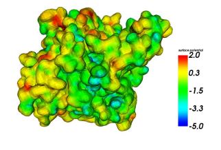
The surface mesh generated by TMSmesh 2.0 can be applied not only to molecular visualization and analysis of surface area, topology and volume in computational structure biology and structural bioinformatics, but also to boundary element method simulations. We test the meshes in boundary element calculations of the Poission-Boltzmann electrostatics. The BEM software used is a publicly available PB solver, AFMPB³⁰. As a representative molecular system, we choose the structure AChE monomer (see Table 1). The surface mesh is generated by TMSmesh 2.0 and contains 87044 nodes. Figure 4 shows the computed electrostatic potentials mapped on the molecular surface.

3.4 Convergence

Figure 5 shows the solvation energies by AFMPB as well as the surface areas and molecular volumes computed from the meshes of three small molecules, GLY, ADP and 2LWC (see Table 1) using different mesh densities. The results show that the meshes produced by TMSmesh 2.0 lead to convergent and reasonable results for energy, area and volume when the mesh density increasing. However, the results computed by MSMS converge a little more smoothly than those of TMSmesh 2.0 when the number of triangles are not large. This is because that we use the trilinear polynomial to approximate the Gaussian kernel function. Less triangles lead to lower precisions of the approximation, which causes more uncertainties. The disparities between the limits when number of triangles goes to large are due to the different molecular surface definitions used by TMSmesh and MSMS.

3.5 Volume Mesh Generation Conforming Surface Mesh

The surface mesh generated by TMSmesh 2.0 can be directly used to generate corresponding surface conforming volume mesh. And the volume mesh generated by this method can be applied to the finie element method simulation directly.

Figure 6 shows a cross section of the volume mesh for the ion channel, VDAC (PDB code: 2JK4). The VDAC serves an essential role in the transport of metabolites and electrolytes between the cell matrix and mitochondria.³¹ For this example, the molecular surface mesh is generated by TMSmesh 2.0 and the corresponding volume mesh is generated by TetGen³². The channel pore is clearly represented in the mesh and the detailed topology is correctly preserved, which is important for ion channel simulations. In addition, from the cross section we can see that the surface mesh is dense at the rugged parts and sparse at the smooth parts.

4 Conclusion

We have described a new algorithm in TMSmesh 2.0 for triangulating the Gaussian molecular surface. In TMSmesh 2.0, an adaptive surface partition is developed using a new method to estimate the upper and lower bounds of surface function in a cell. In each located cube, a trilinear polynomial is used to approximate the Gaussian surface within controllable precision. The fold curves are used to divide the trilinear surface in each cube into single valued pieces to guarantee a manifold mesh generation. Compared with the old version, TMSmesh 2.0 is more than thirty times faster. TMSmesh 2.0 is shown to be a robust and efficient software to mesh the Gaussian molecular surface. The meshes generated by TMSmesh 2.0 are manifold without intersections. And the mesh can be directly used in boundary element type of simulations and volume mesh generations.

5 Acknowledgements

Tiantian Liu and Benzhuo Lu are supported by the State Key Laboratory of Scientific/Engineering Computing, National Center for Mathematics and Interdisciplinary Sciences, Science Challenge Program (SCP) and the China NSF (NSFC 91530102, NSFC 21573274). Minxin Chen is supported by China NSF (NSFC11301368) and the NSF of Jiangsu Province (BK20130278).

References

1 B. Z. Lu, Y. C. Zhou, M. J. Holst, and MaCammon J. A. Recent progress in numerical methods for the Poisson-Boltzmann equation in biophysical applications. Commun. in Comput. Phys., 3(5):973–1009, 2008.
2 M.X. Chen and B.Z. Lu. TMSmesh: A robust method for molecular surface mesh generation using a trace technique. J. Chem. Theory Comput., 7(1):203–212, 2011.
3 M.X. Chen, B. Tu, and B.Z. Lu. Triangulated manifold meshing method preserving molecular surface topology. Journal of Molecular Graphics and Modelling, 38(1):411–418, 2012.
4 B. Lee and F.M. Richards. The interpretation of protein structures: estimation of static accessibility. J. Mol. Biol., 55(3):379–400, 1971.
5 F. M. Richards. Areas, volumes, packing and protein structure. Annual Review in Biophysics and Bioengineering, 6:151–176, 1977.
6 P. W. Bates, G. W. Wei, and Shan Zhao. Minimal molecular surfaces and their applications. Journal of Computational Chemistry, 29(3):380–391, 2008.
7 H. Edelsbrunner. Deformable smooth surface design. Discrete and Computational Geometry, 21(1):87–115, 1999.
8 Tiantian Liu, Minxin Chen, and Benzhuo Lu. Parameterization for molecular gaussian surface and a comparison study of surface mesh generation. Journal of Molecular Modeling, 21(5), 2015.
9 M. L. Connolly. Analytical molecular surface calculation. Journal of Applied Crystallography, 16(5):548–558, 1983.
10 Michael L. Connolly. Solvent-accessible surfaces of proteins and nucleic acids. Science, 221(4612):709–713, 1983.
11 A. Nicholls, R. Bharadwaj, and B. Honig. Grasp:graphical representation and analysis of surface properties. Biophys. J., 64:166–167, 1995.
12 RandyJ. Zauhar. Smart: A solvent-accessible triangulated surface generator for molecular graphics and boundary element applications. Journal of Computer-Aided Molecular Design, 9(2):149–159, 1995.
13 M. Sanner, A. Olson, and J. Spehner. Reduced surface:an efficient way to compute molecular surface properties. Biopolymers, 38(1):305–320, 1996.
14 Y.N. Vorobjev and J. Hermans. Sims: Computation of a smooth invariant molecular surface. Biophysical Journal, pages 722–732, 1997.
15 J. Ryu, R. Park, and D.-S. Kim. Molecular surfaces on proteins via beta shapes. Comput. Aided Des., 39(12):1042–1057, 2007.
16 H. Edelsbrunner and E. P. Mucke. Three-dimensional alpha shapes. ACM Trans Graph, 13:43–72, 1994.
17 Wang YF Can T, Chen CI. Efficient molecular surface generation using level-set methods. Journal of Molecular Graphics and Modelling, 25(1):442–454, 2006.
18 Zhang Y. Xu, D. Generating triangulated macromolecular surfaces by euclidean distance transform. PLoS ONE, 4(12):e8140, 2009.
19 S. Decherchi and W. Rocchia. A general and robust ray casting based algorithm for triangulating surfaces at the nanoscale. PLoS One, 8(4):e59744, 2013.
20 Matthieu Chavent, Bruno Levy, and Bernard Maigret. Metamol: High-quality visualization of molecular skin surface. Journal of Molecular Graphics and Modelling, 27(2):209 – 216, 2008.
21 Ho-Lun Cheng and Xinwei Shi. Quality mesh generation for molecular skin surfaces using restricted union of balls. Computational Geometry, 42(3):196 – 206, 2009.
22 W.E. Lorensen and H. E. Cline. Marching cubes: a high resolution 3d surface construction algorithm. Computer Graphics., 21(4):163–169, 1987.
23 T. Ju, F. Losasso, S. Schaefer, and J. D. Warren. Dual contouring of hermite data. ACM Trans. Graph., 21(3):339–346, 2002.
24 Y.J. Zhang, G.L. Xu, and C. Bajaj. Quality meshing of implicit solvation models of biomolecular structures. Comput. Aided Geom. Des, 23(6):510–530, 2006.
25 Z.Y. Yu, M. J. Holst, and J. McCammon. High-fidelity geometric modeling for biomedical applications. Finite Elem. Anal. Des., 44(11):715–723, 2008.
26 T. Liao, Y.J. Zhang, P. M. Kekenes-Huskey, and et al. Multi-core cpu or gpu-accelerated multiscale modeling for biomolecular complexes. Molecular Based Mathematical Biology, 1(1):164–179, 2013.
27 David Eberly. Triangulation by ear clipping. Geometric Tools, LLC. http://www.geometrictools.com/, 1998.
28 Gary H Meisters. Polygons have ears. American Mathematical Monthly, pages 648–651, 1975.
29 Tamara G. Kolda and Brett W. Bader. Tensor decompositions and applications. SIAM Review, 51(3):455–500, 2009.
30 Bo Zhang, Bo Peng, Jingfang Huang, Nikos P. Pitsianis, Xiaobai Sun, and Benzhuo Lu. Parallel afmpb solver with automatic surface meshing for calculations of molecular solvation free energy. Computer Physics Communications, 190:173–181, 2015.
31 M. Bayrhuber, T. Meins, M. Habeck, S. Becker, K. Giller, S. Villinger, C. Vonrhein, and C. Griesinger. Structure of the human voltage-dependent anion channel. Proc. Natl. Acad. Sci. USA, 105(40):15370–15375, 2008.
32 H. Si. TetGen, a Delaunay-based quality tetrahedral mesh generator. ACM Transactions on Mathematical Software, 41(2):Article 11, 2015.

$\displaystyle\|T(x,y,z)\|$	$\displaystyle=\|R\times_{1}\vec{L}(\frac{2x-(a+b)}{b-a})\times_{2}\vec{L}(\frac{2y-(c+d)}{d-c})\times_{3}\vec{L}(\frac{2z-(e+f)}{f-e})\|$	(40)
	$\displaystyle\leq\|\sum R_{ijk}\|$
	$\displaystyle\leq\sum\|R_{ijk}\|,$

Efficient and Qualified Mesh Generation for Gaussian Molecular Surface Using Piecewise Trilinear Polynomial Approximation

Abstract

1 Introduction

2 Meshing Algorithm

2.1 Algorithm Outline

2.2 Approximating the Gaussian Surface by Piecewise Trilinear Surface

2.2.1 Approximation with nth-degree polynomial

2.2.2 Estimation of upper and lower bound of P~​(x,y,z)\tilde{P}(x,y,z)

2.2.3 Approximation by trilinear polynomial

2.3 Triangulating the trilinear surface

3 Experimental Results

3.1 Efficiency and Robustness

3.2 Manifoldness

3.3 Boundary Element Method Simulation

3.4 Convergence

3.5 Volume Mesh Generation Conforming Surface Mesh

4 Conclusion

5 Acknowledgements

References

2.2.2 Estimation of upper and lower bound of $\tilde{P}(x,y,z)$