跳到论文正文
W Papers独立论文阅读器 arXiv:1611.02874 论文正文 计算阅读时间 · 0%
引用这篇论文根据当前论文元数据生成,正式投稿前建议核对。


License: arXiv.org perpetual non-exclusive license
arXiv:1611.02874v2 [math.ST] 26 Mar 2017

Asymptotic properties of parallel Bayesian kernel density estimators

Alexey Miroshnikov ††thanks: Department of Mathematics, University of California, Los Angeles, amiroshn@gmail.com    Evgeny Savelev ††thanks: Department of Mathematics, Virginia Polytechnic Institute and State University, savelev@vt.edu
Abstract

In this article we perform an asymptotic analysis of Bayesian parallel kernel density estimators introduced by Neiswanger, Wang and Xing [20]. We derive the asymptotic expansion of the mean integrated squared error for the full data posterior estimator and investigate the properties of asymptotically optimal bandwidth parameters. Our analysis demonstrates that partitioning data into subsets requires a non-trivial choice of bandwidth parameters that optimizes the estimation error.

1 Introduction

Recent developments in data science and analytics research have produced an abundance of large data sets that are too large to be analyzed in their entirety. As the size of data sets increases, the time required for processing rises significantly. An effective solution to this problem is to perform statistical analysis of large data sets with the use of parallel computing. The prevalence of parallel processing of large data sets motivated a surge in research on parallel statistical algorithms.

One approach is to divide data sets into smaller subsets, and analyze the subsets on separate machines using parallel Markov chain Monte Carlo (MCMC) methods [15, 19, 26]. These methods, however, require communication between machines for generation of each sample. Communication costs in modern computer networks dwarf the speed up achieved by parallel processing and therefore algorithms that require extensive communications between machined are ineffective; see Scott [25].

To address these issues, numerous alternative communication-free parallel MCMC methods have been developed for Bayesian analysis of big data. These methods partition data into subsets, perform independent Bayesian MCMC analysis on each subset, and combine the subset posterior samples to estimate the full data posterior; see [24, 20, 18].

Neiswanger, Wang and Xing [20] introduced a parallel kernel density estimator that first approximates each subset posterior density; the full data posterior is then estimated by multiplying the subset posterior estimators together,

p^​(𝐱|𝐲)∝p^∗​(𝐱|𝐲):=p^1​(𝐱|𝐲1)⋅p^2​(𝐱|𝐲2)​⋯⋅p^M​(𝐱|𝐲M).{\widehat{p}}({\bf x}|{\bf y})\;\propto\;\displaystyle\widehat{p}^{*}({\bf x}|{\bf y}):={\widehat{p}}_{1}({\bf x}|{\bf y}_{1})\cdot{\widehat{p}}_{2}({\bf x}|{\bf y}_{2})\dots\cdot{\widehat{p}}_{M}({\bf x}|{\bf y}_{M})\,. (1.1)

Here 𝐱∈ℝd{\bf x}\in\mathbb{R}^{d} is the model parameter, 𝐲={𝐲1,𝐲2,…,𝐲M}{\bf y}=\{{\bf y}_{1},{\bf y}_{2},\dots,{\bf y}_{M}\} is the full data set partitioned into MM disjoint independent subsets, and

p^m​(𝐱|𝐲m)=∑i=1Nm1hm​K​(𝐱−𝐗imhm){\widehat{p}}_{m}({\bf x}|{\bf y}_{m})=\sum_{i=1}^{N_{m}}\frac{1}{h_{m}}K\Big(\frac{{\bf x}-{\bf X}_{i}^{m}}{h_{m}}\Big) (1.2)

is the subset posterior kernel density estimator, with hm∈ℝ+h_{m}\in\mathbb{R}_{+} a kernel bandwidth parameter.

The authors of [20] show that the estimator (1.1) is asymptotically exact and develop a sampling algorithm that generates samples from the distribution approximating the full data estimator. Similar sampling algorithms were presented and investigated in Dunson and Wang [21] and Scott [24, 25]. It has been noted that these algorithms do not perform well for posteriors that have non-Gaussian shape and are sensitive to the choice of the kernel parameters; see [18, 24, 21].

The highlighted issues indicate that the proper choice of the bandwidth can greatly benefit the accuracy of the estimation as well as sampling algorithms. Moreover, properly chosen bandwidth parameters will improve accuracy of the estimation without incurring additional computational cost.

In the present article, we are concerned with an asymptotic analysis of the parallel Bayesian kernel density estimators of the form (1.1). In particular, we are interested in the asymptotic representation of the mean integrated squared error (MISE) for the non-normalized estimator p^∗\widehat{p}^{*} and the density estimator p^\widehat{p} as well as the properties of the optimal kernel bandwidth vector parameter 𝐡=(hm)m=1M\mathbf{h}=(h_{m})_{m=1}^{M} as 𝐍=(N1,N2,…,NM)→∞\mathbf{N}=(N_{1},N_{2},\dots,N_{M})\to\infty; the issues left open in [20].

We also propose a universal iterative algorithm based on the derived asymptotic expansions that locates optimal parameters without adopting any assumptions on the underlying probability densities.

The kernel density estimators for the case M=1M=1 have been studied extensively in the past five decades. Asymptotic properties of the mean integrated squared error for the estimator (1.1) with M=1M=1 and d=1d=1, which takes the form (1.2), were studied by Rosenblatt [8], Parzen [10] and Epanechnikov [9]. In particular, for sufficiently smooth probability densities Parzen [10] derived the asymptotic expansion for the mean integrated squared error

MISE​[p,p^,𝐍,𝐡]=h4​k224​∫ℝ(p′′​(x))2​𝑑x+1n​h​∫ℝK2​(t)​𝑑t+o⁡(1n​h+h4),\mbox{\rm MISE}[p,\widehat{p},\mathbf{N},\mathbf{h}]=\frac{h^{4}k^{2}_{2}}{4}\int_{\mathbb{R}}(p^{\prime\prime}(x))^{2}dx+\frac{1}{nh}\int_{\mathbb{R}}K^{2}(t)\,dt+o\Big(\frac{1}{nh}+h^{4}\Big)\,, (1.3)

with 𝐍=n\mathbf{N}=n and 𝐡=h\mathbf{h}=h, and obtained a formula for the asymptotically optimal bandwidth parameter

hM=1opt=n−1/5k2−2/5(∫ℝK2(t)dt)1/5(∫ℝ(p′′(x))2dx)−1/5h^{\rm opt}_{M=1}=n^{-1/5}k_{2}^{-2/5}\left(\int_{\mathbb{R}}K^{2}(t)\,dt\right)^{1/5}\Big(\int_{\mathbb{R}}\big(p^{\prime\prime}(x)\big)^{2}\,dx\Big)^{-1/5}\, (1.4)

which minimizes the leading terms in the expansion.

The case of non-differentiable or discontinuous probability density functions has been shown to possess different asymptotic estimates for MISE. It has been shown by van Eden [7] that the optimal bandwidth parameter hM=1opt∈ℝh_{M=1}^{\rm opt}\in\mathbb{R} and the rate of convergence of the mean integrated squared error depend directly on the regularity of the probability density pp.

In the case of multivariate distributions, d≥1d\geq 1, the complexity of the asymptotic analysis depends on the form of the bandwidth matrix 𝐇∈ℝd×d{\bf H}\in\mathbb{R}^{d\times d}. In the simplest case, one can assume that 𝐇=h​𝐈{\bf H}=h{\bf I}, where hh is a scalar; see Silverman [27], Simonoff [28] and Epanechnikov [9]. Another approach is to consider the bandwidth matrix of the form 𝐇=diag​(h1,h2,…,hd){\bf H}={\text{diag}}(h_{1},h_{2},\dots,h_{d}), with hih_{i} being a bandwidth parameter for each dimension i∈{1,…,d}i\in\{1,\dots,d\}. The most general formulation assumes that 𝐇\mathbf{H} is a d×dd{\times}d matrix, which allows one to encode correlations between components of 𝐱\mathbf{x}; see Duong and Hazelton[6], and Wand and Jones [31].

In the present work, motivated by the ideas of [10, 6, 31, 8] we focus on the case M>1M>1 and d=1d=1 and do the asymptotic analysis of the mean integrated squared error for both the parallel non-normalized estimator

MISE​[p^∗,p∗;𝐍,𝐡]\displaystyle\textstyle\mbox{\rm MISE}\big[\widehat{p}^{*},p^{*}\,;\mathbf{N},\mathbf{h}\big] =𝔼∫ℝ{p∗(x|𝐲)−p^∗(x|𝐲))}2dx\displaystyle=\mathbb{E}\int_{\mathbb{R}}\Big\{p^{*}({x}|{\bf y})-\widehat{p}^{*}({x}|{\bf y}))\Big\}^{2}dx

and the full data set posterior density estimator

MISE​[p^,p;𝐍,𝐡]\displaystyle\textstyle\mbox{\rm MISE}\big[\widehat{p},p\,;\mathbf{N},\mathbf{h}\big] =𝔼∫ℝ{p(x|𝐲)−p^(x|𝐲))}2dx\displaystyle=\mathbb{E}\int_{\mathbb{R}}\Big\{p({x}|{\bf y})-{\widehat{p}}({x}|{\bf y}))\Big\}^{2}dx

as

𝐍=(N1,N2,…,NM)→∞,𝐡=(h1,h2,…,hM)→0and(𝐍⋅𝐡)−1→0.\mathbf{N}=(N_{1},N_{2},\dots,N_{M})\to\infty,\quad{\bf h}=(h_{1},h_{2},\dots,h_{M})\to 0\quad\text{and}\quad(\mathbf{N}\cdot\mathbf{h})^{-1}\to 0.

In Theorem 3.3, under appropriate condition on the regularity of the probability density, we derive the expression for AMISE​[p∗,p^∗]\mbox{\rm AMISE}[p^{*},\widehat{p}^{*}], the asymptotically leading part of MISE for the estimator p^∗\widehat{p}^{*}. The leading part turns out to be in agreement with the leading part for the case M=1M=1, but in the multi-subset case, M>1M>1, the leading part contains novel terms that take into account the relationship between MM subset posterior densities pmp_{m}.

We then perform a similar analysis for the mean square error of the full data set posterior density estimator p^\widehat{p}. The presence of the normalizing constant

c^=λ^−1=(∫p^1​(x|𝐲)⋅p^2​(x|𝐲)​…​p^M​(x|𝐲)​𝑑x)−1=(∫p^∗​(x|𝐲)​𝑑x)−1\widehat{c}=\widehat{\lambda}^{-1}=\bigg(\int\widehat{p}_{1}(x|{\bf y})\cdot\widehat{p}_{2}(x|{\bf y})\dots\widehat{p}_{M}(x|{\bf y})dx\bigg)^{-1}=\bigg(\int\widehat{p}^{*}(x|{\bf y})\,dx\bigg)^{-1}\,

introduces major difficulties in the analysis of MISE because c^\widehat{c} may in general have an infinite second moment in which case MISE​[p^,p]\mbox{\rm MISE}[\widehat{p},p] is not defined. This may occur when the estimators p^i∗\widehat{p}^{*}_{i} (on some events) decay too quickly in xx variable and the sets of xx with the most ‘mass’ for each p^i∗\widehat{p}^{*}_{i} have little common intersection, which potentially leads to large values of c^\widehat{c}. To make sure that 𝔼​c^2<∞\mathbb{E}\widehat{c}^{2}<\infty one must impose appropriate conditions on the density pp and kernel KK. In this article, however, we take another approach. Instead, we replace the mean integrated squared error by an asymptotically equivalent distance functional denoted by

MISE¯​[p^,p;𝐍,𝐡]\displaystyle\textstyle\overline{\mbox{\rm MISE}}\big[\widehat{p},p\,;\mathbf{N},\mathbf{h}\big] =𝔼[(λ^λ)2∫ℝ{p(x|𝐲)−p^(x|𝐲))}2dx].\displaystyle=\mathbb{E}\bigg[\left(\frac{\widehat{\lambda}}{\lambda}\right)^{2}\int_{\mathbb{R}}\Big\{p({x}|{\bf y})-{\widehat{p}}({x}|{\bf y}))\Big\}^{2}dx\bigg].

We show that the new functional is always well-defined and that it is asymptotically equivalent to MISE when restricted to events Ω𝐍⊂Ω\Omega_{\mathbf{N}}\subset\Omega whose probability tends to one as the total number of samples ‖𝐍‖→∞\|\mathbf{N}\|\to\infty.

We then do the analysis of the functional MISE¯\overline{\mbox{\rm MISE}} by carrying out the same program as for the MISE of the estimator p^∗\widehat{p}^{*}. In Theorem 4.6 we derive the expression for AMISE¯​[p,p^]\overline{\mbox{\rm AMISE}}[p,\widehat{p}], the asymptotically leading part of the MISE¯\overline{\mbox{\rm MISE}} for the full data set posterior density estimator p^\widehat{p}. The asymptotically optimal bandwidth parameter for the full data set posterior is then defined to be a minimizer

𝐡opt=argmin𝐡∈ℝ+M​AMISE¯​[p,p^;𝐍,𝐡].{\bf h}^{\rm opt}=\mathrm{argmin}_{\mathbf{h}\in\mathbb{R}^{M}_{+}}\overline{\mbox{\rm AMISE}}[p,\widehat{p};\mathbf{N},\mathbf{h}]\,.

We then compute minimizing bandwidth 𝐡opt{\bf h}^{\rm opt} in explicit form for two special cases. In the examples presented here we consider subset posterior densities of normal and gamma distributions; see (5.2), (5.4), and (5.7). In the two examples the optimizing bandwidth vectors differ significantly and depend, as expected, directly on the full data set density which is typically unknown. For that reason we propose an iterative algorithm for locating optimal bandwidth parameters based on asymptotic expansion we derived; see Algorithm 1.

Our analysis demonstrates that partitioning data into M>1M>1 sets affects the optimality condition of parameter 𝐡{\mathbf{h}}. It also indicates that the bandwidth vector

𝐡0opt=(h1,M=1opt,h2,M=1opt,…,hM,M=1opt),\mathbf{h}^{\rm opt}_{0}=(h^{\rm opt}_{1,M=1},h^{\rm opt}_{2,M=1},\dots,h^{\rm opt}_{M,M=1})\,,

which minimizes the ‘componentwise’ mean integrated squared error

∑i=1MMISE​[p^i,pi,Ni,hi],\sum_{i=1}^{M}\mbox{\rm MISE}[\widehat{p}_{i},p_{i},N_{i},h_{i}]\,,

where hm,M=1opth^{\rm opt}_{m,M=1} is the optimal bandwidth parameter for the estimator p^m​(x|𝐲𝐦)\widehat{p}_{m}(x|{\bf y_{m}}) given by (1.4), is suboptimal for both estimators p^∗\widehat{p}^{*} and p^\widehat{p} whenever M>1M>1.

This observation highlights the fact that the choice of optimal parameters for parallel kernel density estimators (suitable for parallelizing data analysis) must differ from the theoretical choice suggested in case of processing on a single machine. We must also note, that the increased values of MISE resulted from choosing a suboptimal bandwidth parameter get compounded in case of parallel processing. This further necessitates the importance of a proper choice of bandwidth, especially if it comes at no additional computational costs.

The paper is arranged as follows. In Section 2 we set notation and hypotheses that form the foundation of the analysis. In Section 3 we derive an asymptotic expansion for MISE of the non-normalized estimator as well as derive formulas for leading parts of bias​[p^∗]\text{\rm bias}[\widehat{p}^{*}] and 𝕍⁡[p^∗]\mathbb{V}[\widehat{p}^{*}], which are central to the analysis performed in subsequent sections. In Section 4 we perform the analysis of MISE¯\overline{\mbox{\rm MISE}} for the full data set posterior density. In Section 5 we compute explicit expressions for optimal bandwidth parameters for several special cases and conduct numerical experiments. Finally, in the appendix we provide supplementary lemmas and theorems employed in Section 3 and Section 4.

2 Notation and hypotheses

For the convenience of the reader we collect in this section all hypotheses and results relevant to our analysis and present the notation that is utilized throughout the article.

  1. (H1)

    Motivated by the form of the posterior density at Neiswanger et al. [20] we consider the probability density function of the form

    p⁡(x)∝p∗​(x)wherep∗​(x):=∏m=1Mpm​(x)p(x)\propto p^{*}(x)\quad\text{where}\quad p^{*}(x):=\prod_{m=1}^{M}p_{m}(x) (2.1)

    Here pm​(x)p_{m}(x) is a probability density function for each m∈{1,…,M}m\in\{1,\dots,M\} .

  2. (H2)

    We consider the estimator of pp in the form

    p^​(x)∝p^∗​(x)wherep^∗​(x):=∏m=1Mp^m​(x)\hat{p}(x)\propto\displaystyle\hat{p}^{*}(x)\quad\text{where}\quad\hat{p}^{*}(x):=\prod_{m=1}^{M}\hat{p}_{m}(x) (H2-a)

    and for each m∈{1,…,M}m\in\{1,\dots,M\} p^m​(x)\hat{p}_{m}(x) is the kernel density estimator of the probability density pm​(x)p_{m}(x) that has the form

    p^m​(x)=1Nm​hm​∑i=1NmK⁡(x−Ximhm).\hat{p}_{m}(x)=\frac{1}{N_{m}h_{m}}\sum_{i=1}^{N_{m}}K\left(\frac{x-X^{m}_{i}}{h_{m}}\right). (H2-b)

    Here X1m,X2m,…,XNmm∼pm​(x)X_{1}^{m},X_{2}^{m},\dots,X^{m}_{N_{m}}\sim p_{m}(x) are independent identically distributed random variables, KK is a kernel density function, and hm>0h_{m}>0 is a bandwidth parameter.

The mean integrated squared error of the estimator p^∗\widehat{p}^{*} of the non-normalized product p∗p^{*} as well as for the estimator p^​(x)\widehat{p}(x) of the full posterior density p⁡(x)p(x) is defined by

MISE​[p∗,p^∗,𝐍,𝐡]\displaystyle\mbox{\rm MISE}[p^{*},\widehat{p}^{*},\mathbf{N},\mathbf{h}] =MISE​[p∗,p^∗​(x)]:=𝔼​∫ℝ(p^∗​(x)−p∗​(x))2​𝑑x\displaystyle=\mbox{\rm MISE}[p^{*},\widehat{p}^{*}(x)]:=\mathbb{E}\int_{\mathbb{R}}(\widehat{p}^{*}(x)-p^{*}(x))^{2}\,dx (2.2)
MISE​[p,p^,𝐍,𝐡]\displaystyle\mbox{\rm MISE}[p,\widehat{p},\mathbf{N},\mathbf{h}] =MISE​[p,p^​(x)]:=𝔼​∫ℝ(p^​(x)−p⁡(x))2​𝑑x\displaystyle=\mbox{\rm MISE}[p,\widehat{p}(x)]:=\mathbb{E}\int_{\mathbb{R}}(\widehat{p}(x)-p(x))^{2}\,dx

where we use the notation 𝐡=(hm)m=1M\mathbf{h}=(h_{m})_{m=1}^{M} and 𝐍=(Nm)m=1N\mathbf{N}=(N_{m})_{m=1}^{N}. We also use the following convention for the bias and variance of estimators p^​(x),p^∗​(x),p^m​(x)\widehat{p}(x),\widehat{p}^{*}(x),\widehat{p}_{m}(x)

bias​[p^​(x)]\displaystyle\text{\rm bias}[\hat{p}(x)] =𝔼​[p^​(x)]−p​(x)\displaystyle=\mathbb{E}\big[\hat{p}(x)\big]-p(x) (2.3)
bias​[p^∗​(x)]\displaystyle\text{\rm bias}[\hat{p}^{*}(x)] =𝔼⁡[p^∗​(x)]−p∗​(x)\displaystyle=\mathbb{E}\big[\hat{p}^{*}(x)\big]-p^{*}(x)
bias​[p^m​(x)]\displaystyle\text{\rm bias}[\hat{p}_{m}(x)] =𝔼[p^m(x)]−pm(x),m∈{1,…,M}.\displaystyle=\mathbb{E}\big[\hat{p}_{m}(x)\big]-p_{m}(x)\,,\quad m\in\{1,\dots,M\}.

We assume that the kernel density function KK and probability densities functions p1,…,pMp_{1},\dots,p_{M} satisfy the following hypotheses:

  1. (H3)

    KK is positive, bounded, normalized, and its first moment is zero, that is

    0≤K⁡(t)≤C,∫ℝK⁡(t)​𝑑t=1,∫ℝt​K​(t)​𝑑t=0,∫ℝK2​(t)​𝑑t<∞0\leq K(t)\leq C,\quad\int_{\mathbb{R}}K(t)\,dt=1\,,\quad\int_{\mathbb{R}}t\,K(t)\,dt=0\,,\quad\int_{\mathbb{R}}K^{2}(t)\,dt<\infty (2.4)
  2. (H4)

    For each s∈{0,1,2,3}s\in\{0,1,2,3\}

    ks=∫ℝ|t|s​K​(t)​𝑑t<∞.k_{s}=\int_{\mathbb{R}}|t|^{s}K(t)\,dt\,<\,\infty\,. (2.5)
  3. (H5)

    For each m∈{1,…,M}m\in\{1,\dots,M\}, s∈{0,1,2,3}s\in\{0,1,2,3\} and density pm∈C3​(ℝ)p_{m}\in C^{3}(\mathbb{R}) there exists a constant C≥0C\geq 0 such that

    |pm(s)​(x)|<Cfor all ​x∈ℝ.|p_{m}^{(s)}(x)|<C\quad\text{for all }x\in\mathbb{R}\,. (2.6)
  4. (H6)

    For each m∈{1,…,M}m\in\{1,\dots,M\} and s∈{0,1,2,3}s\in\{0,1,2,3\} the density pm​(x)p_{m}(x) and its derivatives are integrable, that is, there is a constant CC so that

    ∫ℝ|pm(s)​(x)|​𝑑x=C<∞.\int_{\mathbb{R}}|p_{m}^{(s)}(x)|\,dx=C<\infty\,. (2.7)
  5. (H7)

    Functions

    𝐍⁡(n)\displaystyle\mathbf{N}(n) ={N1​(n),N2​(n),N3​(n),…,NM​(n)}:ℕ→ℕM\displaystyle=\{N_{1}(n),N_{2}(n),N_{3}(n),\ldots,N_{M}(n)\}:\mathbb{N}\to\mathbb{N}^{M}
    𝐡⁡(n)\displaystyle\mathbf{h}(n) ={h1​(n),h2​(n),…,hM​(n)}:ℕ→ℝ+⁣+M\displaystyle=\{h_{1}(n),h_{2}(n),\ldots,h_{M}(n)\}:\mathbb{N}\to\mathbb{R}_{++}^{M}

    satisfy for all i∈{1,2,…,M}i\in\{1,2,\ldots,M\}

    D1≤Nin≤D2for some ​0<D1<D2\displaystyle D_{1}\leq\frac{N_{i}}{n}\leq D_{2}\quad\text{for some }0<D_{1}<D_{2} (2.8)
    A1​Ni​(n)−α0≤hi​(n)≤A2​Ni​(n)−α0for someα0∈(0,1)\displaystyle A_{1}N_{i}(n)^{-\alpha_{0}}\leq h_{i}(n)\leq A_{2}N_{i}(n)^{-\alpha_{0}}\quad\text{for some}\quad\alpha_{0}\in(0,1)
    limn→∞hi​(n)​Ni​(n)=∞.\displaystyle\lim_{n\to\infty}{h_{i}(n)N_{i}(n)}=\infty\,.

    We also define N¯​(n)=mini⁡Ni​(n)\underline{N}(n)=\min_{i}N_{i}(n) and note that C1​‖𝐍‖≤N¯​(n)≤C2​‖𝐍⁡(n)‖C_{1}\|\mathbf{N}\|\leq\underline{N}(n)\leq C_{2}\|\mathbf{N}(n)\|.

3 Asymptotic analysis of MISE for p^∗\widehat{p}^{*}

We start with the observation that MISE can be expressed via the combination of bias and variance

MISE​[p∗,p^∗]\displaystyle\mbox{\rm MISE}[p^{*},\widehat{p}^{*}] =𝔼​∫ℝ(p^∗​(x)−p∗​(x))2​𝑑x\displaystyle=\mathbb{E}\int_{\mathbb{R}}\big(\widehat{p}^{*}(x)-p^{*}(x)\big)^{2}\,dx (3.1)
=∫ℝ(bias​[p^∗​(x)])2​dx+∫ℝ𝕍⁡[p^∗​(x)]​dx.\displaystyle=\int_{\mathbb{R}}\Big(\text{\rm bias}\big[\widehat{p}^{*}(x)\big]\Big)^{2}\,dx+\int_{\mathbb{R}}\mathbb{V}[\widehat{p}^{*}(x)]\,dx.

In what follows we do the analysis of the bias, then that of variance and conclude with the section where we derive the formula for the optimal bandwidth vector.

3.1 Bias expansion

Using the fact that p^i​(x)\widehat{p}_{i}(x), i=1,…,Mi=1,\dots,M are independent, we obtain

bias​[p^∗​(x)]\displaystyle\text{\rm bias}[\widehat{p}^{*}(x)] =𝔼⁡[p^∗​(x)]−p∗​(x)\displaystyle=\mathbb{E}[\widehat{p}^{*}(x)]-p^{*}(x) (3.2)
=∏m=1M𝔼⁡[p^m]​(x)−∏m=1Mpm​(x)\displaystyle=\prod_{m=1}^{M}\mathbb{E}[\widehat{p}_{m}](x)-\prod_{m=1}^{M}p_{m}(x)
=∏m=1M(bias​[pm​(x)]+pm​(x))−∏m=1Mpm​(x)\displaystyle=\prod_{m=1}^{M}\big(\text{\rm bias}[p_{m}(x)]+p_{m}(x)\big)-\prod_{m=1}^{M}p_{m}(x)

To simplify notation in (3.2) we shall employ the multiindex notation. Let α\alpha be the multiindex with

α=(α1,α2,…,αM)αm∈{0,1}.\alpha=(\alpha_{1},\alpha_{2},\ldots,\alpha_{M})\qquad\alpha_{m}\in\{0,1\}.

Then the above formula can rewritten as follows

bias​[p^∗​(x)]\displaystyle\text{\rm bias}[\widehat{p}^{*}(x)] =∑1⩽|α|⩽M∏m=1Mbiasαm​[p^m​(x)]​(pm​(x))(1−αm)\displaystyle=\sum_{1\leqslant|\alpha|\leqslant M}\prod_{m=1}^{M}\text{\rm bias}^{\alpha_{m}}[\widehat{p}_{m}(x)]\big(p_{m}(x)\big)^{(1-\alpha_{m})} (3.3)
=∑m=1M[bias​[p^m​(x)]​∏k=1k≠mMpk​(x)]\displaystyle=\sum_{m=1}^{M}\left[\text{\rm bias}[\widehat{p}_{m}(x)]\prod_{\begin{subarray}{c}k=1\\ k\neq m\end{subarray}}^{M}p_{k}(x)\right]
+∑2⩽|α|⩽M∏m=1M(bias[p^m(x)])αm(pm(x))(1−αm).\displaystyle+\sum_{2\leqslant|\alpha|\leqslant M}\prod_{m=1}^{M}\big(\text{\rm bias}[\widehat{p}_{m}(x)]\big)^{\alpha_{m}}(p_{m}(x))^{(1-\alpha_{m})}.

Using this decomposition, we prove the following lemma

Lemma 3.1.

Suppose hypotheses (H3)-(H6) hold. Then

  • (i)(i)

    The bias can be expressed as

    bias​[p^∗​(x)]\displaystyle\text{\rm bias}[\widehat{p}^{*}(x)] =k22​∑m=1M[hm2​pm′′​(x)​∏k=1k≠mMpk​(x)]+Eb​(x,𝐡)\displaystyle=\frac{k_{2}}{2}\sum_{m=1}^{M}\left[h_{m}^{2}p_{m}^{\prime\prime}(x)\prod_{\begin{subarray}{c}k=1\\ k\neq m\end{subarray}}^{M}p_{k}(x)\right]+E_{b}(x\hskip 1.0pt;\mathbf{h}) (3.4)

    where the error term Eb​(x,𝐡)E_{b}(x;\mathbf{h}) satisfies the bounds

    |Eb​(x,𝐡)|\displaystyle|E_{b}(x\hskip 1.0pt;\mathbf{h})| ≤E∞​‖𝐡‖3,∀x∈ℝ\displaystyle\leq E_{\infty}||\mathbf{h}||^{3}\,,\quad\forall x\in\mathbb{R} (3.5)
    ∫ℝ|Eb​(x,𝐡)|​𝑑x\displaystyle\int_{\mathbb{R}}|E_{b}(x\hskip 1.0pt;\mathbf{h})|\,dx ≤E1​‖𝐡‖3\displaystyle\leq E_{1}||\mathbf{h}||^{3}
    ∫ℝ|Eb​(x,𝐡)|2​𝑑x\displaystyle\int_{\mathbb{R}}|E_{b}(x\hskip 1.0pt;\mathbf{h})|^{2}\,dx ≤E2​‖𝐡‖6\displaystyle\leq E_{2}||\mathbf{h}||^{6}
  • (i​i)(ii)

    The square-integrated bias satisfies

    ∫ℝbias2​[p^∗​(x)]​𝑑x=k224​∫ℝ[∑m=1Mhm2​pm′′​(x)​∏k=1k≠mMpk​(x)]2​𝑑x+ℰb​(𝐡)<∞\int_{\mathbb{R}}\text{\rm bias}^{2}[\widehat{p}^{*}(x)]\,dx\,=\frac{k_{2}^{2}}{4}\int_{\mathbb{R}}\left[\sum_{m=1}^{M}h_{m}^{2}p_{m}^{\prime\prime}(x)\prod_{\begin{subarray}{c}k=1\\ k\neq m\end{subarray}}^{M}p_{k}(x)\right]^{2}\,dx+\mathcal{E}_{b}(\mathbf{h})\,<\,\infty (3.6)

    with the error term satisfying

    |ℰb​(𝐡)|≤C​‖𝐡‖5|\mathcal{E}_{b}(\mathbf{h})|\leq C||\mathbf{h}||^{5} (3.7)

    where the constant CC is independent of 𝐍\mathbf{N} and 𝐡∈ℝ+M\mathbf{h}\in\mathbb{R}_{+}^{M}.

Proof.

According to (3.3) and (6.2) we have

bias​[p^∗​(x)]=\displaystyle\text{\rm bias}[\widehat{p}^{*}(x)]=
=k22​∑m=1M[hm2​pm′′​(x)​∏k=1k≠mMpk​(x)]+∑m=1M[Eb,m​∏k=1k≠mMpk​(x)]\displaystyle\qquad=\frac{k_{2}}{2}\sum_{m=1}^{M}\left[h_{m}^{2}p^{\prime\prime}_{m}(x)\prod_{\begin{subarray}{c}k=1\\ k\neq m\end{subarray}}^{M}p_{k}(x)\right]+\sum_{m=1}^{M}\left[E_{b,m}\prod_{\begin{subarray}{c}k=1\\ k\neq m\end{subarray}}^{M}p_{k}(x)\right]
+∑2⩽|α|⩽M∏m=1M(hm2​k22pm′′(x)+Eb,m)αm(pm(x))(1−αm)\displaystyle\qquad\qquad+\sum_{2\leqslant|\alpha|\leqslant M}\prod_{m=1}^{M}\left(\frac{h_{m}^{2}k_{2}}{2}p_{m}^{\prime\prime}(x)+E_{b,m}\right)^{\alpha_{m}}(p_{m}(x))^{(1-\alpha_{m})}

Here Eb,mE_{b,m} is the error in bias approximation for each p^m\widehat{p}_{m} from (6.2). We are computing bounds for

Eb​(x,𝐡)=\displaystyle E_{b}(x\hskip 1.0pt;\mathbf{h})= (3.8)
=∑m=1M[Eb,m​∏k=1k≠mMpk​(x)]+∑2⩽|α|⩽M∏m=1M(hm2​k22​pm′′​(x)+Eb,m)αm​(pm​(x))(1−αm)\displaystyle=\sum_{m=1}^{M}\left[E_{b,m}\prod_{\begin{subarray}{c}k=1\\ k\neq m\end{subarray}}^{M}p_{k}(x)\right]+\sum_{2\leqslant|\alpha|\leqslant M}\prod_{m=1}^{M}\left(\frac{h_{m}^{2}k_{2}}{2}p_{m}^{\prime\prime}(x)+E_{b,m}\right)^{\alpha_{m}}(p_{m}(x))^{(1-\alpha_{m})}

To simplify the derivations we separate the terms in (3.8) into two groups: terms with at least one multiple of Eb,mE_{b,m} and terms free of Eb,mE_{b,m}. We define the sets

Am={α=(αj)j=1M:αm=0​ and ​1≤|α|≤(M−1)}A_{m}=\Big\{\alpha=(\alpha_{j})_{j=1}^{M}\ :\ \alpha_{m}=0\text{ and }1\leq|\alpha|\leq(M-1)\Big\} (3.9)

and functions

Pm(x)=∏k=1k≠mMpk(x)+∑α∈Am[∏j=1j≠mM(hj2​k22pj′′(x)+𝟙{j>m}Eb,j)αj(pj(x))(1−αj)].P_{m}(x)=\prod_{\begin{subarray}{c}k=1\\ k\neq m\end{subarray}}^{M}p_{k}(x)+\sum_{\alpha\in A_{m}}\left[\prod_{\begin{subarray}{c}j=1\\ j\neq m\end{subarray}}^{M}\left(\frac{h_{j}^{2}k_{2}}{2}p_{j}^{\prime\prime}(x)+\mathds{1}_{\{j>m\}}E_{b,j}\right)^{\alpha_{j}}(p_{j}(x))^{(1-\alpha_{j})}\right]. (3.10)

Here 𝟙\mathds{1} is the characteristic function. Consequently, the error term can be written as follows

Eb​(x,𝐡)=\displaystyle E_{b}(x\hskip 1.0pt;\mathbf{h})= (3.11)
=∑m=1M[Eb,m​Pm​(x)]+∑2⩽|α|⩽M∏m=1M(hm2​k22​pm′′​(x))αm​(pm​(x))(1−αm).\displaystyle=\sum_{m=1}^{M}\left[E_{b,m}P_{m}(x)\right]+\sum_{2\leqslant|\alpha|\leqslant M}\prod_{m=1}^{M}\left(\frac{h_{m}^{2}k_{2}}{2}p_{m}^{\prime\prime}(x)\right)^{\alpha_{m}}(p_{m}(x))^{(1-\alpha_{m})}.

Assuming that ‖𝐡‖||\mathbf{h}|| is bounded, (H5) and (6.2), we can conclude that there is a constant CPC_{P} so that

|Pm​(x)|≤CP​ for any ​x∈ℝ​ and ​1≤m≤M|P_{m}(x)|\leq C_{P}\text{ for any }x\in\mathbb{R}\text{ and }1\leq m\leq M

Using (H5) and (6.2), we conclude that the first term is bounded, and there is a constant CC so that

∑m=1M|Eb,m​Pm​(x)|≤C​∑m=1M(k3​hm36)≤C​M​‖𝐡‖3​k36.\sum_{m=1}^{M}\left|E_{b,m}P_{m}(x)\right|\leq C\sum_{m=1}^{M}\left(\frac{k_{3}h_{m}^{3}}{6}\right)\leq CM\frac{||\mathbf{h}||^{3}k_{3}}{6}. (3.12)

The next sum in (3.11) contains terms are bounded due to (H5):

|hm2​k22​pm′′​(x)|≤‖𝐡‖2​C​k22and|pm​(x)|≤C\left|\frac{h_{m}^{2}k_{2}}{2}p_{m}^{\prime\prime}(x)\right|\leq\frac{||\mathbf{h}||^{2}Ck_{2}}{2}\qquad\text{and}\qquad|p_{m}(x)|\leq C

For some appropriate constants CC. Since each one of the products below has at least two terms with pm′′​(x)p_{m}^{\prime\prime}(x) for some mm, a constant CQC_{Q} must exist, so that

|∑2⩽|α|⩽M∏m=1M(hm2​k22​pm′′​(x))αm​(pm​(x))(1−αm)|≤CQ​‖𝐡‖4​k224\left|\sum_{2\leqslant|\alpha|\leqslant M}\prod_{m=1}^{M}\left(\frac{h_{m}^{2}k_{2}}{2}p_{m}^{\prime\prime}(x)\right)^{\alpha_{m}}(p_{m}(x))^{(1-\alpha_{m})}\right|\leq C_{Q}\frac{||\mathbf{h}||^{4}k^{2}_{2}}{4} (3.13)

The inequalities (3.12) and (3.13) imply the first inequality in (3.5):

|Eb​(x,𝐡)|≤C​M​‖𝐡‖3​k36+‖𝐡‖4​k224​CQ|E_{b}(x\hskip 1.0pt;\mathbf{h})|\leq CM\frac{||\mathbf{h}||^{3}k_{3}}{6}+\frac{||\mathbf{h}||^{4}k^{2}_{2}}{4}C_{Q} (3.14)

L1L_{1} integrability follows from conditions (H5), (H6), the expansion (3.11) and the second formula in (6.4)

∫ℝ|Eb​(x,𝐡)|​𝑑x≤C⁡(k3​‖𝐡‖36+‖𝐡‖4​k224),\int_{\mathbb{R}}|E_{b}(x\hskip 1.0pt;\mathbf{h})|\,dx\leq C\left(\frac{k_{3}||\mathbf{h}||^{3}}{6}+\frac{||\mathbf{h}||^{4}k_{2}^{2}}{4}\right), (3.15)

which proves the second estimate in (3.5).
Using the estimates obtained above, we conclude

∫ℝ|Eb​(x,𝐡)|2​𝑑x≤supℝ|Eb​(x,𝐡)|⋅∫ℝ|Eb​(x,𝐡)|​𝑑x≤E∞⋅E1​‖𝐡‖6\int_{\mathbb{R}}|E_{b}(x\hskip 1.0pt;{\bf h})|^{2}\,dx\leq\sup_{\mathbb{R}}|E_{b}(x\hskip 1.0pt;{\bf h})|\cdot\int_{\mathbb{R}}|E_{b}(x\hskip 1.0pt;{\bf h})|\,dx\leq E_{\infty}\cdot E_{1}||\mathbf{h}||^{6}

Finally, (ii) follows from Cauchy-Schwartz inequality applied to

bias2​[p^∗​(x)]\displaystyle\text{\rm bias}^{2}[\widehat{p}^{*}(x)] =k224​[∑m=1Mhm2​pm′′​(x)​∏k=1k≠mMpk​(x)]2+\displaystyle=\frac{k_{2}^{2}}{4}\left[\sum_{m=1}^{M}h_{m}^{2}p_{m}^{\prime\prime}(x)\prod_{\begin{subarray}{c}k=1\\ k\neq m\end{subarray}}^{M}p_{k}(x)\right]^{2}+
+Eb​(x,𝐡)​k2​[∑m=1Mhm2​pm′′​(x)​∏k=1k≠mMpk​(x)]+Eb2​(x,𝐡)\displaystyle+E_{b}(x\hskip 1.0pt;\mathbf{h})k_{2}\left[\sum_{m=1}^{M}h_{m}^{2}p_{m}^{\prime\prime}(x)\prod_{\begin{subarray}{c}k=1\\ k\neq m\end{subarray}}^{M}p_{k}(x)\right]+E_{b}^{2}(x\hskip 1.0pt;\mathbf{h})

which leads directly to (3.6) and (3.7) ∎

3.2 Variance expansion

We next obtain an asymptotic formula for the variance of p^∗\hat{p}^{*}. For the proof of the lemma, we perform the following preliminary calculation

𝕍​[p^∗​(x)]\displaystyle\mathbb{V}[\widehat{p}^{*}(x)] =𝔼⁡[(p^∗​(x))2]−(𝔼⁡[p^∗​(x)])2=∏m=1M𝔼⁡[p^m2]−∏m=1M𝔼2​[p^m]\displaystyle=\mathbb{E}[(\widehat{p}^{*}(x))^{2}]-\Big(\mathbb{E}[\widehat{p}^{*}(x)]\Big)^{2}=\prod_{m=1}^{M}\mathbb{E}[\widehat{p}_{m}^{2}]-\prod_{m=1}^{M}\mathbb{E}^{2}[\widehat{p}_{m}] (3.16)
=∏m=1M(𝕍⁡[p^m]+(pm+bias​[p^m])2)−∏m=1M(pm+bias​[p^m])2\displaystyle=\prod_{m=1}^{M}\Big(\mathbb{V}[\widehat{p}_{m}]+\big(p_{m}+\text{\rm bias}[\widehat{p}_{m}]\big)^{2}\Big)-\prod_{m=1}^{M}\Big(p_{m}+\text{\rm bias}[\widehat{p}_{m}]\Big)^{2}
=∑1⩽|α|⩽M∏m=1M(𝕍⁡[p^m])αm​(pm+bias​[p^m])2​(1−αm)\displaystyle=\sum_{1\leqslant|\alpha|\leqslant M}\prod_{m=1}^{M}\big(\mathbb{V}[\widehat{p}_{m}]\big)^{\alpha_{m}}\big(p_{m}+\text{\rm bias}[\widehat{p}_{m}]\big)^{2(1-\alpha_{m})}
Lemma 3.2.

Let hypotheses (H3)-(H7) hold. Then

  • (i)(i)

    The variation of p^∗\hat{p}^{*} is given by

    𝕍⁡[p^∗​(x)]=(∑m=1M[pmNm​hm​∏k=1k≠mMpk2​(x)])​∫ℝK2​(t)​𝑑t+EV​(x,𝐍,𝐡),x∈ℝ\mathbb{V}[\hat{p}^{*}(x)]=\left(\sum_{m=1}^{M}\left[\frac{p_{m}}{N_{m}h_{m}}\prod_{\begin{subarray}{c}k=1\\ k\neq m\end{subarray}}^{M}p_{k}^{2}(x)\right]\right)\int_{\mathbb{R}}K^{2}(t)\,dt+E_{V}(x\hskip 1.0pt;\mathbf{N},\mathbf{h})\,,\quad x\in\mathbb{R} (3.17)

    where the error term EV​(x,n,𝐡)E_{V}(x\hskip 1.0pt;n,\mathbf{h}) satisfies the bounds

    |ℰV​(N,h)|\displaystyle|\mathcal{E}_{V}(N,h)| :=|∫ℝEV​(x)​dx|=o⁡(1‖𝐍‖)\displaystyle:=\left|\int_{\mathbb{R}}E_{V}(x)\,dx\right|=o\left(\frac{1}{\|\mathbf{N}\|}\right) (3.18)
Proof.

According to (3.16) we have

𝕍​(p^∗​(x))=\displaystyle\mathbb{V}(\hat{p}^{*}(x))= (3.19)
=∑1⩽|α|⩽M∏m=1M(pm​(x)Nm​hm​∫ℝK2​(t)​𝑑t+EV,m)αm​(pm+bias​[p^m])2​(1−αm)\displaystyle=\sum_{1\leqslant|\alpha|\leqslant M}\prod_{m=1}^{M}\left(\frac{p_{m}(x)}{N_{m}h_{m}}\int_{\mathbb{R}}K^{2}(t)\,dt+E_{V,m}\right)^{\alpha_{m}}\big(p_{m}+\text{\rm bias}[\widehat{p}_{m}]\big)^{2(1-\alpha_{m})}
=∑1⩽|α|⩽M∏m=1M(pm​(x)Nm​hm​∫ℝK2​(t)​𝑑t+EV,m)αm​(pm2+2​pm​bias​[p^m]+bias2​[p^m])(1−αm)\displaystyle=\sum_{1\leqslant|\alpha|\leqslant M}\prod_{m=1}^{M}\left(\frac{p_{m}(x)}{N_{m}h_{m}}\int_{\mathbb{R}}K^{2}(t)\,dt+E_{V,m}\right)^{\alpha_{m}}\big(p_{m}^{2}+2p_{m}\,\text{\rm bias}[\widehat{p}_{m}]+\text{\rm bias}^{2}[\widehat{p}_{m}]\big)^{(1-\alpha_{m})}

Here, EV,mE_{V,m} is the approximation error of variance of each pm​(x)p_{m}(x) from (6.11). In a fashion similar to the previous proof, we separate the terms in (3.19). We single out the leading order terms, the terms with at least one multiple of EV,mE_{V,m}, the terms with multiples of bias​[p^m]\text{\rm bias}[\widehat{p}_{m}] and the terms of the order o⁡(1‖𝐍‖​‖𝐡‖)o\left(\frac{1}{\|\mathbf{N}\|\|\mathbf{h}\|}\right).

We define sets

Am0\displaystyle A^{0}_{m} ={α=(αj)j=1M:αm=0​ and ​0≤|α|≤(M−1)}\displaystyle=\Big\{\alpha=(\alpha_{j})_{j=1}^{M}\ :\ \alpha_{m}=0\text{ and }0\leq|\alpha|\leq(M-1)\Big\} (3.20)
Bm1\displaystyle B^{1}_{m} ={α=(αj)j=1M:αm=0​ and ​|α|=1}\displaystyle=\Big\{\alpha=(\alpha_{j})_{j=1}^{M}\ :\ \alpha_{m}=0\text{ and }|\alpha|=1\Big\}

and functions

Pm0​(x)\displaystyle P^{0}_{m}(x) =∑α∈Am0[∏j=1j≠mM(pm​(x)Nm​hm∫ℝK2(t)dt+𝟙{j>m}EV,m)αm(𝔼2[p^m])(1−αm)],\displaystyle=\sum_{\alpha\in A^{0}_{m}}\left[\prod_{\begin{subarray}{c}j=1\\ j\neq m\end{subarray}}^{M}\left(\frac{p_{m}(x)}{N_{m}h_{m}}\int_{\mathbb{R}}K^{2}(t)\,dt+\mathds{1}_{\{j>m\}}E_{V,m}\right)^{\alpha_{m}}\big(\mathbb{E}^{2}[\widehat{p}_{m}]\big)^{(1-\alpha_{m})}\right], (3.21)
Qm1​(x)\displaystyle Q^{1}_{m}(x) =∑α∈Bm1[∏j=1j≠mM(pm​(x)Nm​hm​∫ℝK2​(t)​dt)αm​(𝔼2​[p^m])(1−αm)],\displaystyle=\sum_{\alpha\in B^{1}_{m}}\left[\prod_{\begin{subarray}{c}j=1\\ j\neq m\end{subarray}}^{M}\left(\frac{p_{m}(x)}{N_{m}h_{m}}\int_{\mathbb{R}}K^{2}(t)\,dt\right)^{\alpha_{m}}\big(\mathbb{E}^{2}[\widehat{p}_{m}]\big)^{(1-\alpha_{m})}\right],

The variance expansion can be rewritten as

𝕍​(p^∗​(x))=\displaystyle\mathbb{V}(\hat{p}^{*}(x))= (3.22)
=∑1⩽|α|⩽M∏m=1M(pm​(x)Nm​hm​∫ℝK2​(t)​𝑑t)αm​(pm2+2​pm​bias​[p^m]+bias2​[p^m])(1−αm)\displaystyle=\sum_{1\leqslant|\alpha|\leqslant M}\prod_{m=1}^{M}\left(\frac{p_{m}(x)}{N_{m}h_{m}}\int_{\mathbb{R}}K^{2}(t)\,dt\right)^{\alpha_{m}}\big(p_{m}^{2}+2p_{m}\,\text{\rm bias}[\widehat{p}_{m}]+\text{\rm bias}^{2}[\widehat{p}_{m}]\big)^{(1-\alpha_{m})}
+∑m=1MEV,mP0m(x)\displaystyle+\sum_{m=1}^{M}E_{V,m}P^{0}_{m}(x)
=∑m=1M(pm​(x)Nm​hm​∫ℝK2​(t)​dt)​∏j=1j≠mMpm2​(x)\displaystyle=\sum_{m=1}^{M}\left(\frac{p_{m}(x)}{N_{m}h_{m}}\int_{\mathbb{R}}K^{2}(t)\,dt\right)\prod_{\begin{subarray}{c}j=1\\ j\neq m\end{subarray}}^{M}p_{m}^{2}(x)
+∑m=1Mbias[p^m](2pm(x)+bias[p^m])Qm1(x)\displaystyle+\sum_{m=1}^{M}\text{\rm bias}[\widehat{p}_{m}](2p_{m}(x)+\text{\rm bias}[\widehat{p}_{m}])Q_{m}^{1}(x)
+∑2⩽|α|⩽M∏m=1M(pm​(x)Nm​hm∫ℝK2(t)dt)αm(𝔼2[p^m])(1−αm)\displaystyle+\sum_{2\leqslant|\alpha|\leqslant M}\prod_{m=1}^{M}\left(\frac{p_{m}(x)}{N_{m}h_{m}}\int_{\mathbb{R}}K^{2}(t)\,dt\right)^{\alpha_{m}}\big(\mathbb{E}^{2}[\widehat{p}_{m}]\big)^{(1-\alpha_{m})}
+∑m=1MEV,mP0m(x)\displaystyle+\sum_{m=1}^{M}E_{V,m}P^{0}_{m}(x)

Based on definitions of functions Pm0​(x)P^{0}_{m}(x) and Qm1​(x)Q^{1}_{m}(x), hypotheses (H5), (H6) and (H7) we can conclude that there are constants C𝔼,CP,CQC_{\mathbb{E}},C_{P},C_{Q} so that

𝔼⁡[p^m]\displaystyle\mathbb{E}[\widehat{p}_{m}] ≤C𝔼\displaystyle\leq C_{\mathbb{E}}
|Pm0​(x)|\displaystyle|P_{m}^{0}(x)| ≤CP\displaystyle\leq C_{P}
|Qm1​(x)|\displaystyle|Q^{1}_{m}(x)| ≤CQ​1‖𝐍‖​‖𝐡‖\displaystyle\leq C_{Q}\frac{1}{\|\mathbf{N}\|\|\mathbf{h}\|}

Therefore

∫ℝ|EV​(x)|​𝑑x\displaystyle\int_{\mathbb{R}}|E_{V}(x)|dx (3.23)
≤∑m=1MC⁡(2+‖𝐡‖2​k22)​CQ‖𝐍‖​‖𝐡‖​∫ℝ|bias​[p^m]|​𝑑x\displaystyle\leq\sum_{m=1}^{M}C\left(2+\frac{||\mathbf{h}||^{2}k_{2}}{2}\right)\frac{C_{Q}}{\|\mathbf{N}\|\|\mathbf{h}\|}\int_{\mathbb{R}}|\text{\rm bias}[\widehat{p}_{m}]|dx
+1‖𝐍‖2​‖𝐡‖2∑2⩽|α|⩽M(1‖𝐍‖2​‖𝐡‖2)(|α|−2)C𝔼(M−|α|)\displaystyle+\frac{1}{\|\mathbf{N}\|^{2}\|\mathbf{h}\|^{2}}\sum_{2\leqslant|\alpha|\leqslant M}\left(\frac{1}{\|\mathbf{N}\|^{2}\|\mathbf{h}\|^{2}}\right)^{(|\alpha|-2)}C_{\mathbb{E}}^{(M-|\alpha|)}
+M⋅CP‖𝐍‖\displaystyle+\frac{M\cdot C_{P}}{\|\mathbf{N}\|}

This leads directly to (3.18). ∎

3.3 AMISE formula and optimal bandwidth vector

With the lemmas above we can derive the decomposition of MISE​[p∗,p^∗]\mbox{\rm MISE}[p^{*},\widehat{p}^{*}] into leading order terms and higher order terms.

Theorem 3.3.

Let hypotheses (H3)-(H7) hold. Then MISE can be represented as

MISE​[p∗,p^∗,𝐍,𝐡]=AMISE​[p∗,p^∗,𝐍,𝐡]+ℰ⁡(𝐍,𝐡)\displaystyle\mbox{\rm MISE}[p^{*},\widehat{p}^{*},\mathbf{N},\mathbf{h}]=\mbox{\rm AMISE}[p^{*},\widehat{p}^{*},\mathbf{N},\mathbf{h}]+\mathcal{E}(\mathbf{N},\mathbf{h}) (3.24)

where the leading term

AMISE​[p∗,p^∗;𝐍,𝐡]\displaystyle\mbox{\rm AMISE}[p^{*},\widehat{p}^{*};\mathbf{N},\mathbf{h}] =k224​∫ℝ(∑m=1M[hm2​pm′′​(x)​∏k=1k≠mMpk​(x)])2​dx+\displaystyle=\frac{k_{2}^{2}}{4}\int_{\mathbb{R}}\left(\sum_{m=1}^{M}\left[h_{m}^{2}p_{m}^{\prime\prime}(x)\prod_{\begin{subarray}{c}k=1\\ k\neq m\end{subarray}}^{M}p_{k}(x)\right]\right)^{2}\,dx+ (3.25)
+∫ℝ(∑m=1M[pm​(x)Nm​hm∏k=1k≠mM(pk(x))2])dx∫ℝK2(t)dt\displaystyle+\int_{\mathbb{R}}\left(\sum_{m=1}^{M}\left[\frac{p_{m}(x)}{N_{m}h_{m}}\prod_{\begin{subarray}{c}k=1\\ k\neq m\end{subarray}}^{M}(p_{k}(x))^{2}\right]\right)dx\int_{\mathbb{R}}K^{2}(t)\,dt

and the error term ℰ\mathcal{E} satisfies

ℰ⁡(𝐍,𝐡)=ℰb​(𝐍,𝐡)+ℰV​(𝐍,𝐡)=o⁡(‖𝐡‖4+1‖𝐍‖​‖𝐡‖)\mathcal{E}(\mathbf{N},\mathbf{h})=\mathcal{E}_{b}(\mathbf{N},\mathbf{h})+\mathcal{E}_{V}(\mathbf{N},\mathbf{h})=o\Big(||\mathbf{h}||^{4}+\frac{1}{\|\mathbf{N}\|\|\mathbf{h}\|}\Big) (3.26)

as 𝐡→0\mathbf{h}\to 0, 𝐍→∞\mathbf{N}\to\infty, and (‖𝐍‖​‖𝐡‖)−1→0(\|\mathbf{N}\|\|\mathbf{h}\|)^{-1}\to 0.

Proof.

The result follows from Lemma 3.1, Lemma 3.2, and formula (3.1) ∎

Remark 3.4.

We would like to note that the analysis we perform here is in spirit of the asymptotic analysis performed for multivariate kernel density estimators by Epanechnikov [9]. However, the full-data set density pp under consideration is a univariate density expressed as a product and cannot be viewed as a special case of the expansion obtained in [9].

Remark 3.5.

The asymptotically leading part derived here is the first step of our analysis. It serves as a stepping stone for the analysis of full MISE carried out in the next section. We would like to note that one can find optimal bandwidth that minimizes AMISE for the non-normalized estimator. One has to be aware, however, that these optimal parameters would not take into account a normalization constant and, as a consequence, would be suboptimal for MISE of the normalized full data set density p^\widehat{p}.

4 Asymptotic analysis of MISE for p^\widehat{p}

4.1 Normalizing constant

In this section we consider the error that arises when one takes into account the normalizing constant. Recall that by assumption

p⁡(x)∝p∗​(x)wherep∗​(x):=∏m=1Mpm​(x)p(x)\propto p^{*}(x)\quad\text{where}\quad p^{*}(x):=\prod_{m=1}^{M}p_{m}(x)

where pm​(x)p_{m}(x), m∈{1,…,M}m\in\{1,\dots,M\} is a probability density function. Then we define

λ:=∫p∗​(x)​𝑑x>0andc:=λ−1\lambda:=\int p^{*}(x)\,dx>0\quad\text{and}\quad c:=\lambda^{-1} (4.1)

and obtain p⁡(x)=c​p∗​(x)p(x)=cp^{*}(x). For the estimator

p^​(x)∝p^∗​(x)withp^∗​(x):=∏m=1Mp^m​(x)\hat{p}(x)\propto\displaystyle\hat{p}^{*}(x)\quad\text{with}\quad\hat{p}^{*}(x):=\prod_{m=1}^{M}\hat{p}_{m}(x)

we similarly define

λ^:=∫p^∗​(x)​𝑑x>0andc^:=λ^−1\widehat{\lambda}:=\int\widehat{p}^{*}(x)\,dx>0\quad\text{and}\quad\widehat{c}:=\widehat{\lambda}^{-1} (4.2)

and hence p^​(x)=c^​p^∗​(x)\widehat{p}(x)=\widehat{c}\widehat{p}^{*}(x).

We are interested in the optimal bandwidth vector 𝐡=(h)m=1M\mathbf{h}=(h)_{m=1}^{M} that optimizes the leading term of the mean integrated squared error

MISE​(p^,p)=MISE​(c^​p^∗,c​p∗)=𝔼​∫ℝ(c​p∗​(x)−c^​p^∗​(x))2​𝑑x.\mbox{\rm MISE}(\hat{p},\,p)=\mbox{\rm MISE}(\widehat{c}\widehat{p}^{*},\,cp^{*})=\mathbb{E}\int_{\mathbb{R}}\big(cp^{*}(x)-\widehat{c}\widehat{p}^{*}(x)\big)^{2}\,dx\,. (4.3)

Observe that c^\widehat{c} and p^∗\widehat{p}^{*} are not independent and the previously performed analysis is not directly applicable. Moreover, we observe that the estimator of the normalizing constant

c^=(∫∏i=1Mp^i​(x)​𝑑x)−1<∞\widehat{c}=\bigg(\int\prod_{i=1}^{M}\widehat{p}_{i}(x)\,dx\bigg)^{-1}<\infty (4.4)

may in general have an infinite expectation. This may happen because the estimators in the above product may decay too quickly in xx variable and the sets of xx with the most ‘mass’ for each pip_{i} may have no common intersection. This potentially may lead to small values of λ^\widehat{\lambda} and hence large c^\widehat{c}. To avoid this situation one would need to chose the kernel KK in appropriate way and establish the finiteness of the expectation of c^\widehat{c}.

In this article we do not investigate this. Instead, we will show that one can replace MISE by an equivalent functional which is well-defined and finite on the whole sample space Ω\Omega and that there exists a sequence of smaller sample subspaces Ωn\Omega_{n} with ℙ⁡(Ωn)→1\mathbb{P}(\Omega_{n})\to 1 , on which the new functional is asymptotically equivalent to MISE​[p,p^]\mbox{\rm MISE}[p,\widehat{p}] restricted to Ωn\Omega_{n}. We then analyze the new functional and investigate its optimal parameters.

4.2 Preliminary estimates

Lemma 4.1 (covariance).

Let p^∗​(x)\widehat{p}^{*}(x) be an estimator of the form (H2-a) where the vector of sample sizes 𝐍⁡(n)\mathbf{N}(n) and bandwidth vector 𝐡⁡(n)\mathbf{h}(n) satisfy (H7). Then

Cov​[p^∗​(x),p^∗​(y)]=𝔼⁡[p^∗​(x)​p^∗​(y)]−𝔼⁡[p^∗​(x)]​𝔼​[p^∗​(y)]\mbox{\rm Cov}[\widehat{p}^{*}(x),\widehat{p}^{*}(y)]=\mathbb{E}[\widehat{p}^{*}(x)\widehat{p}^{*}(y)]-\mathbb{E}[\widehat{p}^{*}(x)]\mathbb{E}[\widehat{p}^{*}(y)] (4.5)

satisfies the estimates

|Cov​[p^∗​(x),p^∗​(y)]|\displaystyle|\mbox{\rm Cov}[\widehat{p}^{*}(x),\widehat{p}^{*}(y)]| ≤Ca​b​s‖𝐍‖​‖𝐡‖\displaystyle\leq\frac{C_{abs}}{\|\mathbf{N}\|\|\mathbf{h}\|} (4.6)
|∬Cov​[p^∗​(x),p^∗​(y)]​dx​dy|\displaystyle\left|\iint\mbox{\rm Cov}[\widehat{p}^{*}(x),\widehat{p}^{*}(y)]\,dxdy\right| ≤Ci​n​t‖𝐍‖\displaystyle\leq\frac{C_{int}}{\|\mathbf{N}\|}

for some constants Ca​b​s,Ci​n​t>0C_{abs},C_{int}>0 independent of nn.

Proof.

We can expand the product as follows

∏i=1M𝔼⁡[p^i​(x)​p^i​(y)]−∏i=1M𝔼⁡[p^i​(x)]​𝔼​[p^i​(y)]\displaystyle\prod_{i=1}^{M}\mathbb{E}[\widehat{p}_{i}(x)\widehat{p}_{i}(y)]-\prod_{i=1}^{M}\mathbb{E}[\widehat{p}_{i}(x)]\mathbb{E}[\widehat{p}_{i}(y)]
=∑j=1M(​𝔼​[p^j​(x)​p^j​(y)]−𝔼⁡[p^j​(x)]​𝔼​[p^j​(y)])​(∏i=1j−1𝔼⁡[p^i​(x)​p^i​(y)])​(∏i=j+1M𝔼⁡[p^i​(x)]​𝔼​[p^i​(y)])\displaystyle=\sum_{j=1}^{M}\left(\rule{0.0pt}{10.00002pt}\mathbb{E}[\widehat{p}_{j}(x)\widehat{p}_{j}(y)]-\mathbb{E}[\widehat{p}_{j}(x)]\mathbb{E}[\widehat{p}_{j}(y)]\right)\left(\prod_{i=1}^{j-1}\mathbb{E}[\widehat{p}_{i}(x)\widehat{p}_{i}(y)]\right)\left(\prod_{i=j+1}^{M}\mathbb{E}[\widehat{p}_{i}(x)]\mathbb{E}[\widehat{p}_{i}(y)]\right)

where the products with the top index smaller than the bottom index should be taken as having the value one.

We next observe that, according to (6.2), for each i∈{1,…,M}i\in\{1,\dots,M\}

|𝔼⁡[p^i​(x)]​𝔼​[p^i​(y)]|≤C​(1+k2​hi22+k3​hi36)2.|\mathbb{E}[\widehat{p}_{i}(x)]\mathbb{E}[\widehat{p}_{i}(y)]|\leq C\left(1+\frac{k_{2}h_{i}^{2}}{2}+\frac{k_{3}h_{i}^{3}}{6}\right)^{2}\,.

Also Lemma 6.4 implies that

|𝔼⁡[p^i​(x)​p^i​(y)]|≤C​(1+k2​hi22+k3​hi36)2+CNi​hi+CNi​(1+(1+k2​hi22+k3​hi36)2)\Big|\mathbb{E}[\widehat{p}_{i}(x)\widehat{p}_{i}(y)]\Big|\leq C\left(1+\frac{k_{2}h_{i}^{2}}{2}+\frac{k_{3}h_{i}^{3}}{6}\right)^{2}+\frac{C}{N_{i}h_{i}}+\frac{C}{N_{i}}\left(1+\left(1+\frac{k_{2}h_{i}^{2}}{2}+\frac{k_{3}h_{i}^{3}}{6}\right)^{2}\right)

Then we conclude that for some C𝔼≥0C_{\mathbb{E}}\geq 0

|𝔼⁡[p^i​(x)​p^i​(y)]|,|𝔼⁡[p^i​(x)]​𝔼​[p^i​(y)]|\displaystyle|\mathbb{E}[\widehat{p}_{i}(x)\widehat{p}_{i}(y)]|,|\mathbb{E}[\widehat{p}_{i}(x)]\mathbb{E}[\widehat{p}_{i}(y)]| ≤C𝔼<∞,for allx,y∈ℝ.\displaystyle\leq C_{\mathbb{E}}<\infty\,,\quad\text{for all}\quad x,y\in\mathbb{R}\,.

Therefore, by Lemma 6.4 we obtain the estimate

|Cov​[p^∗​(x),p^∗​(y)]|≤M​C​(1‖𝐍‖​‖𝐡‖+1‖𝐍‖​(1+(1+k2​‖𝐡‖22+k3​‖𝐡‖36)2))|\mbox{\rm Cov}[\widehat{p}^{*}(x),\widehat{p}^{*}(y)]|\leq M\,C\left(\frac{1}{\|\mathbf{N}\|\|\mathbf{h}\|}+\frac{1}{\|\mathbf{N}\|}\left(1+\left(1+\frac{k_{2}\|\mathbf{h}\|^{2}}{2}+\frac{k_{3}\|\mathbf{h}\|^{3}}{6}\right)^{2}\right)\right)

for some appropriate constant CC, which gives (4.6)1.

The integral of Cov​[p^∗​(x),p^∗​(y)]\mbox{\rm Cov}[\widehat{p}^{*}(x),\widehat{p}^{*}(y)] is also finite. Using the result of Lemma 6.4 and the hypothesis (H6)

∬|Cov​[p^∗​(x),p^∗​(y)]|​𝑑x​𝑑y\displaystyle\iint\Big|\mbox{\rm Cov}\big[\widehat{p}^{*}(x),\widehat{p}^{*}(y)\big]\Big|\,dxdy
≤C𝔼M−1​∑i=1M∬|​𝔼​[p^j​(x)​p^j​(y)]−𝔼⁡[p^j​(x)]​𝔼​[p^j​(y)]|​𝑑x​𝑑y\displaystyle\leq C_{\mathbb{E}}^{M-1}\sum_{i=1}^{M}\iint\left|\rule{0.0pt}{10.00002pt}\mathbb{E}[\widehat{p}_{j}(x)\widehat{p}_{j}(y)]-\mathbb{E}[\widehat{p}_{j}(x)]\mathbb{E}[\widehat{p}_{j}(y)]\right|\,dxdy
≤C𝔼M−1​∑i=1M∬(1Ni​pi​(x)​1hi​K2​(x−yhi)+|EΠ,i​(x,y)|)​𝑑x​𝑑y\displaystyle\leq C_{\mathbb{E}}^{M-1}\sum_{i=1}^{M}\iint\left(\frac{1}{N_{i}}p_{i}(x)\frac{1}{h_{i}}K_{2}\left(\frac{x-y}{h_{i}}\right)+|E_{\Pi,i}(x,y)|\right)\,dxdy
≤C𝔼M−1​M‖𝐍‖​(2+C⁡(k1+k2​‖𝐡‖22+k3​‖𝐡‖36)),\displaystyle\leq C_{\mathbb{E}}^{M-1}\frac{M}{\|\mathbf{N}\|}\left(2+C\left(k_{1}+\frac{k_{2}\|\mathbf{h}\|^{2}}{2}+\frac{k_{3}\|\mathbf{h}\|^{3}}{6}\right)\right),

Where at the last step we used the facts that 1h​K2​(x−yh)\frac{1}{h}K_{2}\left(\frac{x-y}{h}\right) is a probability density function in yy for any fixed xx and pi​(x)p_{i}(x) is also a probability density function.

∎

Lemma 4.2.

Let p^∗​(x)\widehat{p}^{*}(x) be an estimator of the form (H2-a) where the vector of sample sizes 𝐍⁡(n)\mathbf{N}(n) and bandwidth vector 𝐡⁡(n)\mathbf{h}(n) satisfy (H7). Then following identity and the estimate holds

𝕍⁡[λ^−λ]=𝕍⁡[∫p^∗​(x)​dx−∫p∗​(x)​dx]≤Ci​n​t‖𝐍‖<∞,\displaystyle\mathbb{V}[\widehat{\lambda}-\lambda]=\mathbb{V}\Big[\int\widehat{p}^{*}(x)\,dx-\int p^{*}(x)\,dx\Big]\leq\frac{C_{int}}{\|\mathbf{N}\|}<\infty,

where Ci​n​t>0C_{int}>0 is defined in (4.6).

Proof.

Since λ\lambda is constant we have

𝕍⁡[λ^−λ]\displaystyle\mathbb{V}[\widehat{\lambda}-\lambda] =𝔼​[λ^−𝔼⁡[λ^]]2\displaystyle=\mathbb{E}\big[\widehat{\lambda}-\mathbb{E}[\widehat{\lambda}]\big]^{2}
=𝔼​[∫ℝp^∗​(x)−𝔼⁡[p^∗​(x)]​dx]2\displaystyle=\mathbb{E}\left[\int_{\mathbb{R}}\widehat{p}^{*}(x)-\mathbb{E}[\widehat{p}^{*}(x)]\,dx\right]^{2}
=𝔼⁡[∫(p^∗​(x)−𝔼⁡[p^∗​(x)])​dx⋅∫(p^∗​(y)−𝔼⁡[p^∗​(y)])​dy]\displaystyle=\mathbb{E}\left[\int\left(\widehat{p}^{*}(x)-\mathbb{E}[\widehat{p}^{*}(x)]\right)dx\cdot\int\left(\widehat{p}^{*}(y)-\mathbb{E}[\widehat{p}^{*}(y)]\right)dy\right]
=∬(𝔼⁡[p^∗​(x)​p^∗​(y)]−𝔼⁡[p^∗​(x)]​𝔼​[p^∗​(y)])​dx​dy≤Ci​n​t‖𝐍‖,\displaystyle=\iint\Big(\mathbb{E}\left[\widehat{p}^{*}(x)\widehat{p}^{*}(y)\right]-\mathbb{E}[\widehat{p}^{*}(x)]\mathbb{E}[\widehat{p}^{*}(y)]\Big)dx\,dy\leq\frac{C_{int}}{\|\mathbf{N}\|},

where the last inequality is from Lemma 4.1. ∎

Lemma 4.3.

Let p^∗​(x)\widehat{p}^{*}(x) be an estimator of the form (H2-a) where the vector of sample sizes 𝐍⁡(n)\mathbf{N}(n) and bandwidth vector 𝐡⁡(n)\mathbf{h}(n) satisfy (H7). Then for any α∈(0,1]\alpha\in(0,1]

ℙ⁡({ω:|𝔼​λ^−λ^​(ω,𝐍⁡(n),𝐡⁡(n))|>λ2​‖𝐍‖1−α2})≤2​Ci​n​tλ2​‖𝐍‖α.\mathbb{P}\bigg(\bigg\{\omega:|\mathbb{E}{\widehat{\lambda}}-\widehat{\lambda}(\omega;\mathbf{N}(n),\mathbf{h}(n))|>\frac{{\lambda}}{\sqrt{2}{\|\mathbf{N}\|}^{\frac{1-\alpha}{2}}}\bigg\}\bigg)\leq\frac{2C_{int}}{\lambda^{2}{\|\mathbf{N}\|}^{\alpha}}\,. (4.7)

Moreover, for any α\alpha satisfying

max⁡(0,1−4​α0)<α<1,\max(0,1-4\alpha_{0})<\alpha<1\,,

where α0\alpha_{0} is defined in (H7) , we have

ℙ{|λ^λ−1|>1‖𝐍‖1−α2}≤2​Ci​n​tλ2​‖𝐍‖α.\mathbb{P}\bigg\{\Big|\frac{\widehat{\lambda}}{\lambda}-1\Big|>\frac{1}{\|\mathbf{N}\|^{\frac{1-\alpha}{2}}}\bigg\}\leq\frac{2C_{int}}{\lambda^{2}\|\mathbf{N}\|^{\alpha}}\,. (4.8)

for all sufficiently large nn.

Proof.

By Lemma 4.2 and Chebyshev inequality we obtain

ℙ{|λ^−𝔼[λ^]|2>λ22​‖𝐍‖1−α}\displaystyle\mathbb{P}\bigg\{\big|\widehat{\lambda}-\mathbb{E}[\widehat{\lambda}]\big|^{2}>\frac{\lambda^{2}}{2{\|\mathbf{N}\|}^{1-\alpha}}\bigg\}
≤ℙ{|λ^−𝔼[λ^]|2>𝕍(λ^)λ2​‖𝐍‖α2​Ci​n​t}≤2​Ci​n​tλ2​‖𝐍‖α.\displaystyle\leq\mathbb{P}\bigg\{\big|\widehat{\lambda}-\mathbb{E}[\widehat{\lambda}]\big|^{2}>\mathbb{V}(\widehat{\lambda})\frac{\lambda^{2}{\|\mathbf{N}\|}^{\alpha}}{2C_{int}}\bigg\}\leq\frac{2C_{int}}{\lambda^{2}{\|\mathbf{N}\|}^{\alpha}}\,.

Recall next that

|𝔼⁡(λ^)−λ|=|∫(𝔼⁡[p^∗​(x)]−p∗​(x))​𝑑x|≤∫|bias​[p^∗]|​𝑑x≤C​‖𝐡‖2|\mathbb{E}(\widehat{\lambda})-\lambda|=\Big|\int\Big(\mathbb{E}[\widehat{p}^{*}(x)]-p^{*}(x)\Big)\,dx\Big|\leq\int|\text{\rm bias}[\widehat{p}^{*}]|\,dx\leq C\|\mathbf{h}\|^{2}

where CC is independent of 𝐡\mathbf{h}. According to (H7) we have ‖𝐡⁡(n)‖≤A​‖𝐍‖−α0\|\mathbf{h}(n)\|\leq A\|\mathbf{N}\|^{-\alpha_{0}} for some α0∈(0,1)\alpha_{0}\in(0,1). Fix an arbitrary α\alpha that satisfies

max⁡(0,1−4​α0)<α⁡<1so that4​α0>​1−α.\max(0,1-4\alpha_{0})<\alpha<1\quad\text{so that}\quad 4\alpha_{0}>1-\alpha.

Then

‖𝐡‖2​‖𝐍‖1−α2≤A​‖𝐍‖−2​α0​‖𝐍‖1−α2=A​‖𝐍‖−4​α0+(1−α)2→0as n→∞{\|\mathbf{h}\|^{2}}{\|\mathbf{N}\|^{\frac{1-\alpha}{2}}}\leq{A\|\mathbf{N}\|^{-2\alpha_{0}}}{\|\mathbf{N}\|^{\frac{1-\alpha}{2}}}=A\|\mathbf{N}\|^{\frac{-4\alpha_{0}+(1-\alpha)}{2}}\to 0\quad\text{as $n\to\infty$}

Thus there exists n0n_{0} such that

C​‖𝐡⁡(n)‖2<λ4​‖𝐍⁡(n)‖−(1−α)2for all n>n0.C\|\mathbf{h}(n)\|^{2}<\frac{\lambda}{4}\|\mathbf{N}(n)\|^{-\frac{(1-\alpha)}{2}}\quad\text{for all $n>n_{0}$}\,. (4.9)

By the triangle inequality we have

|λ^−𝔼​λ^|>|λ^−λ|−|λ−𝔼​λ^|>|λ^−λ|−λ4​‖𝐍‖−(1−α)2\displaystyle\big|\widehat{\lambda}-\mathbb{E}\widehat{\lambda}\big|>\big|\widehat{\lambda}-\lambda\big|-\big|\lambda-\mathbb{E}\widehat{\lambda}\big|>\big|\widehat{\lambda}-\lambda\big|-\frac{\lambda}{4}\|\mathbf{N}\|^{-\frac{(1-\alpha)}{2}}

and hence for every

ω0∈{ω:|λ^​(ω)−λ|>λ‖𝐍‖1−α2}\omega_{0}\in\Big\{\omega:\,|\widehat{\lambda}({\omega})-\lambda|>\frac{\lambda}{\|\mathbf{N}\|^{\frac{1-\alpha}{2}}}\Big\} (4.10)

we have

|λ^​(ω0)−𝔼​λ^|\displaystyle\big|\widehat{\lambda}(\omega_{0})-\mathbb{E}\widehat{\lambda}\big| >|λ^​(ω0)−λ|−λ4​‖𝐍‖−(1−α)2>3​λ4​‖𝐍‖−(1−α)2>λ2​‖𝐍‖−(1−α)2.\displaystyle>\big|\widehat{\lambda}(\omega_{0})-\lambda\big|-\frac{\lambda}{4}\|\mathbf{N}\|^{-\frac{(1-\alpha)}{2}}>\frac{3\lambda}{4}\|\mathbf{N}\|^{-\frac{(1-\alpha)}{2}}>\frac{\lambda}{\sqrt{2}}\|\mathbf{N}\|^{-\frac{(1-\alpha)}{2}}\,. (4.11)

Then (4.10) and (4.11) we obtain

{ω:|λ^​(ω)−λ|>λ‖𝐍‖1−α2}⊂{ω:|λ^​(ω)−𝔼​λ^|>λ2​‖𝐍‖1−α2}\Big\{{\omega}:\,|\widehat{\lambda}({\omega})-\lambda|>\frac{\lambda}{\|\mathbf{N}\|^{\frac{1-\alpha}{2}}}\Big\}\subset\Big\{{\omega}:\,|\widehat{\lambda}({\omega})-\mathbb{E}\widehat{\lambda}|>\frac{\lambda}{\sqrt{2}\|\mathbf{N}\|^{\frac{1-\alpha}{2}}}\Big\}

and hence

ℙ⁡{ω:|λ^​(ω)−λ|>λ‖𝐍‖1−α2}\displaystyle\mathbb{P}\Big\{{\omega}:\,|\widehat{\lambda}({\omega})-\lambda|>\frac{\lambda}{\|\mathbf{N}\|^{\frac{1-\alpha}{2}}}\Big\} (4.12)
≤ℙ⁡{ω:|λ^​(ω)−𝔼​λ^|>λ2​‖𝐍‖1−α2}≤2​Ci​n​tλ2​‖𝐍‖α.\displaystyle\leq\mathbb{P}\Big\{{\omega}:\,|\widehat{\lambda}({\omega})-\mathbb{E}\widehat{\lambda}|>\frac{\lambda}{\sqrt{2}\|\mathbf{N}\|^{\frac{1-\alpha}{2}}}\Big\}\leq\frac{2C_{int}}{\lambda^{2}\|\mathbf{N}\|^{\alpha}}\,.

∎

4.3 Functional equivalent to MISE

As it was pointed the functional MISE defined in (4.3) is not defined in the whole space Ω\Omega because the reciprocal of the renormalization random variable (λ^)−1(\widehat{\lambda})^{-1} may in general have en infinite expectation.

The event space Ωn\Omega_{n} insures that the constant c^\widehat{c} has a finite expectation and stays close to the true normalization constant cc. However, even on this smaller and safer space the functional MISE​[p^,p]\mbox{\rm MISE}[\widehat{p},p] is rather difficult to analyze. To help resolve this issue we introduce a functional that is asymptotically equivalent to MISE on the space Ωn\Omega_{n}

Definition 4.4.
MISE¯=𝔼⁡[(λ^λ)2​∫ℝ(p^​(x)−p⁡(x))2​𝑑x]\overline{\mbox{\rm MISE}}=\mathbb{E}\left[\left(\frac{\widehat{\lambda}}{\lambda}\right)^{2}\int_{\mathbb{R}}(\widehat{p}(x)-p(x))^{2}dx\,\right] (4.13)

The equivalence follows from the definition of the space Ωn\Omega_{n}

Proposition 4.5.

The functional MISE¯{\overline{\mbox{\rm MISE}}} is asymptotically equivalent to MISE on smaller events Ωn\Omega_{n} uniformly in nn, that is

lim‖𝐍⁡(n)‖→∞MISE¯[p(x),p^(x;ω)|ω∈Ωn]MISE[p(x),p^(x;ω)|ω∈Ωn]=1\lim_{\|\mathbf{N}(n)\|\to\infty}\frac{\overline{\mbox{\rm MISE}}[p(x),\widehat{p}(x;\omega)|\omega\in\Omega_{n}\big]}{\mbox{\rm MISE}[p(x),\widehat{p}(x;\omega)|\omega\in\Omega_{n}\big]}=1 (4.14)

where

Ωn={ω∈Ω:|λ^−λ|≤λ‖𝐍‖1−α2}withℙ⁡(Ωn)≥1−C‖𝐍‖α\Omega_{n}=\bigg\{\omega\in\Omega:\,|\widehat{\lambda}-\lambda|\leq\frac{\lambda}{\|\mathbf{N}\|^{\frac{1-\alpha}{2}}}\bigg\}\quad\text{with}\quad\mathbb{P}(\Omega_{n})\geq 1-\frac{C}{\|\mathbf{N}\|^{\alpha}} (4.15)

and α\alpha is a fixed constant satisfying 1>α>min⁡(1−4​α0,0)1>\alpha>\min(1-4\alpha_{0},0).

Proof.

Observe that

MISE¯[p(x),p^(x)|Ωn]=1ℙ⁡(Ωn)∫Ωn(λ^λ)2∫ℝ(p^(x,ω)−p(x))2dxℙ(dω)\displaystyle\overline{\mbox{\rm MISE}}[p(x),\widehat{p}(x)|\Omega_{n}\big]=\frac{1}{\mathbb{P}(\Omega_{n})}\int_{\Omega_{n}}\left(\frac{\widehat{\lambda}}{\lambda}\right)^{2}\int_{\mathbb{R}}(\widehat{p}(x,\omega)-p(x))^{2}dx\,\mathbb{P}(d\omega)
=1ℙ⁡(Ωn)​(∫Ωn[(λ^λ−1)2+2​(λ^λ−1)+1]​∫ℝ(p^​(x,ω)−p⁡(x))2​dx)​ℙ​(dω).\displaystyle=\frac{1}{\mathbb{P}(\Omega_{n})}\bigg(\int_{\Omega_{n}}\left[\left(\frac{\widehat{\lambda}}{\lambda}-1\right)^{2}+2\left(\frac{\widehat{\lambda}}{\lambda}-1\right)+1\right]\int_{\mathbb{R}}(\widehat{p}(x,\omega)-p(x))^{2}dx\,\bigg)\mathbb{P}(d\omega).

Then by (4.15) we obtain that

MISE¯[p(x),p^(x)|Ωn]=(1+ε(n))MISE[p(x),p^(x)|Ωn]\overline{\mbox{\rm MISE}}[p(x),\widehat{p}(x)|\Omega_{n}\big]=(1+\varepsilon(n))\mbox{\rm MISE}[p(x),\widehat{p}(x)|\Omega_{n}\big]

where

|ε⁡(n)|≤C‖𝐍‖1−α2,|\varepsilon(n)|\leq\frac{C}{\|\mathbf{N}\|^{\frac{1-\alpha}{2}}},

for some constant C>0C>0 independent of nn. This implies (4.14). ∎

One of the positive side effects we must mention is that the functional defined in (4.13) is not only easier to analyze but also it is defined throughout the whole space Ω\Omega. We take advantage of this fact and continue the discussion with expectations taken over the whole unrestricted space.

With the slight modification of the functional we can now extract the leading order part

Theorem 4.6.

The distance functional MISE¯\overline{\mbox{\rm MISE}} can be represented as

MISE¯​[p,p^,𝐍,𝐡]=AMISE¯​[p,p^,𝐍,𝐡]+ℰ⁡(𝐍,𝐡)\displaystyle\overline{\mbox{\rm MISE}}[p,\widehat{p},\mathbf{N},\mathbf{h}]=\overline{\mbox{\rm AMISE}}[p,\widehat{p},\mathbf{N},\mathbf{h}]+\mathcal{E}(\mathbf{N},\mathbf{h}) (4.16)

where the leading term

AMISE¯​[p,p^,𝐍,𝐡]\displaystyle\overline{\mbox{\rm AMISE}}[p,\widehat{p},\mathbf{N},\mathbf{h}] :=(∫B⁡(x)​𝑑x)2​∫(c​p∗​(x))2​𝑑x\displaystyle:=\left(\int B(x)\,dx\right)^{2}\int\big(cp^{*}(x)\big)^{2}\,dx (4.17)
+∫(B(x))2dx+∫ℝ(V(x))dx∫ℝK2(t)dt\displaystyle+\int\left(B(x)\right)^{2}dx+\int_{\mathbb{R}}\left(V(x)\right)dx\int_{\mathbb{R}}K^{2}(t)\,dt
−2∬B(y)B(x)cp∗(x)dxdy\displaystyle-2\iint B(y)\,B(x)\,cp^{*}(x)\,dx\,dy
B⁡(x)\displaystyle B(x) =c​k22​∑m=1M[hm2​pm′′​(x)​∏k=1k≠mMpk​(x)]\displaystyle=\frac{ck_{2}}{2}\sum_{m=1}^{M}\left[h_{m}^{2}p_{m}^{\prime\prime}(x)\prod_{\begin{subarray}{c}k=1\\ k\neq m\end{subarray}}^{M}p_{k}(x)\right]
V⁡(x)\displaystyle V(x) =∑m=1M[pmNm​hm​∏k=1k≠mMpk2​(x)]\displaystyle=\sum_{m=1}^{M}\left[\frac{p_{m}}{N_{m}h_{m}}\prod_{\begin{subarray}{c}k=1\\ k\neq m\end{subarray}}^{M}p_{k}^{2}(x)\right]

and the error term ℰ\mathcal{E} satisfies

ℰ⁡(𝐍,𝐡)=o⁡(‖𝐡‖4+1‖𝐍‖​‖𝐡‖)\mathcal{E}(\mathbf{N},\mathbf{h})=o\Big(||\mathbf{h}||^{4}+\frac{1}{\|\mathbf{N}\|\|\mathbf{h}\|}\Big) (4.18)

as 𝐡→0\mathbf{h}\to 0, 𝐍→∞\mathbf{N}\to\infty, and (‖𝐍‖​‖𝐡‖)−1→0(\|\mathbf{N}\|\|\mathbf{h}\|)^{-1}\to 0.

Proof.

We can divide the functional MISE¯\overline{\mbox{\rm MISE}} into three components

MISE¯​[p,p^]\displaystyle\overline{\mbox{\rm MISE}}[p,\widehat{p}] =J1+J2+J3\displaystyle=J_{1}+J_{2}+J_{3} (4.19)
=c2​𝔼​[(λ−λ^)2]​∫ℝ(p⁡(x))2​𝑑x\displaystyle=c^{2}\mathbb{E}[(\lambda-\widehat{\lambda})^{2}]\int_{\mathbb{R}}\left(p(x)\right)^{2}dx
+c2𝔼∫ℝ(p^∗−p∗)2dx\displaystyle+c^{2}\mathbb{E}\int_{\mathbb{R}}(\widehat{p}^{*}-p^{*})^{2}dx
−2c2𝔼∫ℝ(λ^−λ)(p^∗−p∗)p(x)dx.\displaystyle-2c^{2}\mathbb{E}\int_{\mathbb{R}}(\widehat{\lambda}-\lambda)(\widehat{p}^{*}-p^{*})p(x)\,dx.

Our first step will be to express each term JiJ_{i}, i=1,…,3, as a sum of a higher order term and the term containing a bias, variance or their combination. We then will use the results of the previous section and the appendix to obtain a leading part of each term.

First observe that

𝔼⁡[(λ−λ^)2]\displaystyle\mathbb{E}[(\lambda-\widehat{\lambda})^{2}] =𝔼⁡[(λ−𝔼⁡[λ^])2]+𝔼⁡[(𝔼⁡[λ^]−λ^)2]\displaystyle=\mathbb{E}[(\lambda-\mathbb{E}[\widehat{\lambda}])^{2}]+\mathbb{E}[(\mathbb{E}[\widehat{\lambda}]-\widehat{\lambda})^{2}]
=(𝔼⁡[∫p⁡(x)−p^​(x)​dx])2+𝔼⁡[(𝔼⁡[λ^]−λ^)2].\displaystyle=\bigg(\mathbb{E}\bigg[\int p(x)-\widehat{p}(x)\,dx\bigg]\bigg)^{2}+\mathbb{E}[(\mathbb{E}[\widehat{\lambda}]-\widehat{\lambda})^{2}].

The second term turns out to be of higher order. This can be seen from the following estimate

𝔼⁡[(λ^−𝔼⁡[λ^])2]=𝔼​[∫(p^∗−𝔼​p^∗)​dx]2\displaystyle\mathbb{E}[(\widehat{\lambda}-\mathbb{E}[\widehat{\lambda}])^{2}]=\mathbb{E}\left[\int\left(\widehat{p}^{*}-\mathbb{E}\widehat{p}^{*}\right)dx\right]^{2} (4.20)
=𝔼⁡[∫(p^∗−𝔼​p^∗)​dx⋅∫(p^∗−𝔼​p^∗)​dx]\displaystyle=\mathbb{E}\left[\int\left(\widehat{p}^{*}-\mathbb{E}\widehat{p}^{*}\right)dx\cdot\int\left(\widehat{p}^{*}-\mathbb{E}\widehat{p}^{*}\right)dx\right]
=𝔼⁡[∫(p^∗​(x)−𝔼​p^∗​(x))​dx⋅∫(p^∗​(y)−𝔼​p^∗​(y))​dy]\displaystyle=\mathbb{E}\left[\int\left(\widehat{p}^{*}(x)-\mathbb{E}\widehat{p}^{*}(x)\right)dx\cdot\int\left(\widehat{p}^{*}(y)-\mathbb{E}\widehat{p}^{*}(y)\right)dy\right]
=∬(𝔼⁡[p^∗​(x)​p^∗​(y)]−𝔼⁡[p^∗​(x)]​𝔼​[p^∗​(y)])​𝑑x​𝑑y≤C1‖𝐍‖\displaystyle=\iint\left(\mathbb{E}\left[\widehat{p}^{*}(x)\widehat{p}^{*}(y)\right]-\mathbb{E}[\widehat{p}^{*}(x)]\mathbb{E}[\widehat{p}^{*}(y)]\right)dx\,dy\leq\frac{C_{1}}{\|\mathbf{N}\|}

where the last inequality follows from Lemma 4.1.

Thus, we conclude

J1=c2​(∫bias​[p∗,p^∗]​𝑑x)2​∫(p⁡(x))2​𝑑x+E1where ​|E1|≤C‖𝐍‖.J_{1}=c^{2}\left(\int\text{\rm bias}[p^{*},\widehat{p}^{*}]\,dx\right)^{2}\int\big(p(x)\big)^{2}\,dx+E_{1}\quad\text{where }|E_{1}|\leq\frac{C}{\|\mathbf{N}\|}.

From (3.1) we have that

J2=c2​∫(bias2​[p∗,p^∗]+𝕍⁡[p^∗])​𝑑x.J_{2}=c^{2}\int\bigg(\text{\rm bias}^{2}[p^{*},\widehat{p}^{*}]+\mathbb{V}[\widehat{p}^{*}]\bigg)\,dx.

The term J3J_{3} can be expressed as

J3=c2​𝔼n​∬(p^∗​(y)−p∗​(y))​((p^∗​(x)−p∗​(x))​p​(x))​𝑑y​𝑑x\displaystyle J_{3}=c^{2}\mathbb{E}_{n}\iint\big(\widehat{p}^{*}(y)-p^{*}(y)\big)\Big(\big(\widehat{p}^{*}(x)-p^{*}(x)\big)p(x)\Big)\,dydx
=c2​∬bias​[p^∗​(y)]​bias​[p^∗​(x)]​p​(x)​𝑑x​𝑑y\displaystyle=c^{2}\iint\text{\rm bias}[\widehat{p}^{*}(y)]\text{\rm bias}[\widehat{p}^{*}(x)]\,p(x)\,dx\,dy
+c2𝔼∬(𝔼[p^∗(y)]−p^∗(y))(𝔼[p^∗(x)]−p^∗(x))p(x)dydx\displaystyle+c^{2}\mathbb{E}\iint\big(\mathbb{E}[\widehat{p}^{*}(y)]-\widehat{p}^{*}(y)\big)\big(\mathbb{E}[\widehat{p}^{*}(x)]-\widehat{p}^{*}(x)\big)p(x)\,dydx

Since p∗​(x)p^{*}(x) is uniformly bounded, Lemma 4.1 implies that the last term in the above identity satisfies

|c2​𝔼​∬(𝔼⁡[p^∗​(y)]−p^∗​(y))​(𝔼⁡[p^∗​(x)]−p^∗​(x))​c​p∗​(x)​𝑑y​𝑑x|≤C‖𝐍‖.\left|c^{2}\mathbb{E}\iint\big(\mathbb{E}[\widehat{p}^{*}(y)]-\widehat{p}^{*}(y)\big)\big(\mathbb{E}[\widehat{p}^{*}(x)]-\widehat{p}^{*}(x)\big)cp^{*}(x)\,dydx\right|\leq\frac{C}{\|\mathbf{N}\|}.

This gives

J3=c2∬bias[p^∗(y)]bias[p^∗(x)]p(x)dxdy+E3,|E3|<1‖𝐍‖.\displaystyle J_{3}=c^{2}\iint\text{\rm bias}[\widehat{p}^{*}(y)]\text{\rm bias}[\widehat{p}^{*}(x)]\,p(x)\,dx\,dy+E_{3},\quad|E_{3}|<\frac{1}{\|\mathbf{N}\|}\,.

Combining the above estimates gives

MISE¯​[p,p^]\displaystyle\overline{\mbox{\rm MISE}}\big[p,\widehat{p}\big] =c2​(∫bias​[p∗,p^∗]​𝑑x)2​∫(p⁡(x))2​𝑑x\displaystyle=c^{2}\left(\int\text{\rm bias}[p^{*},\widehat{p}^{*}]\,dx\right)^{2}\int\big(p(x)\big)^{2}\,dx (4.21)
+c2∫bias2[p∗,p^∗]+𝕍[p^∗]dx\displaystyle+c^{2}\int\text{\rm bias}^{2}[p^{*},\widehat{p}^{*}]+\mathbb{V}[\widehat{p}^{*}]\,dx
−2c2∬bias[p^∗(y)]bias[p^∗(x)]p(x)dxdy+EM,|EM|≤C‖𝐍‖\displaystyle-2c^{2}\iint\text{\rm bias}[\widehat{p}^{*}(y)]\text{\rm bias}[\widehat{p}^{*}(x)]\,p(x)\,dx\,dy+E_{M},\quad|E_{M}|\leq\frac{C}{\|\mathbf{N}\|}

Applying the results of Lemma 3.1 and Lemma 3.2 to the identity (4.21) leads to (4.16) and (4.17) and this finishes the proof.

∎

4.4 Numerical optimization scheme for optimal bandwidth

In the absence of knowledge of probability density functions p⁡(x)p(x) and pm​(x)p_{m}(x), it may seem that the formula (4.17) has little practical use. However, we can replace the densities with their approximations p^​(x)\widehat{p}(x) and p^m​(x)\widehat{p}_{m}(x). This will turn the quantity AMISE¯\overline{\mbox{\rm AMISE}} into a function of the form

AMISE¯​(𝐡)=∑i,j=1Mhi2​hj2​βi,j+∑i=1Mνihi{\overline{\mbox{\rm AMISE}}}(\mathbf{h})=\sum_{i,j=1}^{M}h_{i}^{2}h_{j}^{2}\beta_{i,j}+\sum_{i=1}^{M}\frac{\nu_{i}}{h_{i}} (4.22)

where

βi,j\displaystyle\beta_{i,j} =c^2​k224​∫ℝp^i′′​(x)​∏k=1k≠iMp^k​(x)​𝑑x​∫ℝp^j′′​(x)​∏k=1k≠jMp^k​(x)​𝑑x​∫ℝp^2​(x)​𝑑x\displaystyle=\frac{\widehat{c}^{2}k^{2}_{2}}{4}\int_{\mathbb{R}}\widehat{p}_{i}^{\prime\prime}(x)\prod_{\begin{subarray}{c}k=1\\ k\neq i\end{subarray}}^{M}\widehat{p}_{k}(x)\,dx\int_{\mathbb{R}}\widehat{p}_{j}^{\prime\prime}(x)\prod_{\begin{subarray}{c}k=1\\ k\neq j\end{subarray}}^{M}\widehat{p}_{k}(x)\,dx\int_{\mathbb{R}}\widehat{p}^{2}(x)\,dx (4.23)
+c^2​k224∫ℝ(p^i′′(x)∏k=1k≠iMp^k(x))(p^j′′(x)∏k=1k≠jMp^k(x))dx\displaystyle+\frac{\widehat{c}^{2}k^{2}_{2}}{4}\int_{\mathbb{R}}\left(\widehat{p}_{i}^{\prime\prime}(x)\prod_{\begin{subarray}{c}k=1\\ k\neq i\end{subarray}}^{M}\widehat{p}_{k}(x)\right)\left(\widehat{p}_{j}^{\prime\prime}(x)\prod_{\begin{subarray}{c}k=1\\ k\neq j\end{subarray}}^{M}\widehat{p}_{k}(x)\right)dx
−c^2​k222∫ℝp^i′′(y)∏k=1k≠iMp^k(y)dy∫ℝp^j′′(x)∏k=1k≠jMp^k(x)p^(x)dx\displaystyle-\frac{\widehat{c}^{2}k^{2}_{2}}{2}\int_{\mathbb{R}}\widehat{p}_{i}^{\prime\prime}(y)\prod_{\begin{subarray}{c}k=1\\ k\neq i\end{subarray}}^{M}\widehat{p}_{k}(y)\,dy\int_{\mathbb{R}}\widehat{p}_{j}^{\prime\prime}(x)\prod_{\begin{subarray}{c}k=1\\ k\neq j\end{subarray}}^{M}\widehat{p}_{k}(x)\widehat{p}(x)\,dx
νi\displaystyle\nu_{i} =∫ℝp^iNi​∏k=1k≠iMp^k2​(x)​𝑑x​∫ℝK2​(t)​𝑑t\displaystyle=\int_{\mathbb{R}}\frac{\widehat{p}_{i}}{N_{i}}\prod_{\begin{subarray}{c}k=1\\ k\neq i\end{subarray}}^{M}\widehat{p}_{k}^{2}(x)\,dx\int_{\mathbb{R}}K^{2}(t)\,dt

This can be used to create an iterative algorithm that will yield a near optimal value for 𝐡\mathbf{h}. A possible implementation of such an algorithm is laid out in Algorithm 1.

Algorithm 1 Locate optimal bandwidth vector 𝐡=(h1,…,hM)\mathbf{h}=(h_{1},\ldots,h_{M})

input: Samples Xi,mX_{i,m}
result: Vector 𝐡=(h1,h2,…,hM)\mathbf{h}=(h_{1},h_{2},\ldots,h_{M})


1: Initialize k=0k=0, 𝐡0\mathbf{h}_{0} with hi=hopth_{i}=h^{\rm opt} from (5.4)
2: repeat
3:   Increment kk
4:   Compute estimators p^m\widehat{p}_{m}, p^∗\widehat{p}^{*} and c^\widehat{c}
5:   Compute βi,j\beta_{i,j} and νi\nu_{i} from (4.23)
6:   Compute 𝐡k+1\mathbf{h}_{k+1} by executing a few steps of the gradient (or conjugate gradient) descent minimization algorithm applied to AMISE¯​(𝐡)\overline{\mbox{\rm AMISE}}(\mathbf{h})
7: until ‖𝐡k−𝐡k+1‖\|\mathbf{h}_{k}-\mathbf{h}_{k+1}\| is sufficiently small

The conditions, under which the iterative algorithm 1 will converge to the minimizing vector hopth^{\rm opt}, need to be thoroughly investigated. Such investigation is outside the limits of this publication and is one of the directions of the future work the authors consider.

5 Examples

In a general setting, finding a bandwidth vector 𝐡\mathbf{h} that minimizes (4.17) would require solving a system of nonlinear equations, which would probably not have a closed form solution and require application of numerical methods. In this section we discuss two special cases, for which closed form solutions can be obtained with relative ease.

5.1 AMISE¯\overline{\mbox{\rm AMISE}} optimization for a symmetric case

In this case we assume that all posterior densities for each subset of samples are the same, and that all subsets contain the same number of samples. In other words we employ the following assumptions

  • •

    p1​(x)=p2​(x)=⋯=pM​(x)=f⁡(x)p_{1}(x)=p_{2}(x)=\dots=p_{M}(x)=f(x).

  • •

    N1=N2=⋯=NMN_{1}=N_{2}=\dots=N_{M}, that is, 𝐍=(n,n,…,n)\mathbf{N}=(n,n,\dots,n), for some n∈ℕn\in\mathbb{N}

In view of the symmetry, all components of the optimal bandwidth vector should be the same, that is 𝐡=(h,h,…,h)\mathbf{h}=(h,h,\dots,h). Under these assumptions, the expression for AMISE¯\overline{\mbox{\rm AMISE}} simplifies into

AMISE¯[p(x),p^(x)|𝐍,𝐡]:=M2c2​k22​h44(∫p1′′(x)p1M−1(x)dx)2∫(cp1M(x))2dx\displaystyle\overline{\mbox{\rm AMISE}}[p(x),\widehat{p}(x)|\mathbf{N},\mathbf{h}]:=M^{2}\frac{c^{2}k^{2}_{2}h^{4}}{4}\left(\int p_{1}^{\prime\prime}(x)p_{1}^{M-1}(x)\,dx\right)^{2}\int\big(cp_{1}^{M}(x)\big)^{2}\,dx (5.1)
+M2c2​k22​h44∫(p1′′(x)p1M−1(x))2dx+M∫ℝ(p12​M−1n​h)dx∫ℝK2(t)dt\displaystyle+M^{2}\frac{c^{2}k^{2}_{2}h^{4}}{4}\int\left(p_{1}^{\prime\prime}(x)p_{1}^{M-1}(x)\right)^{2}dx+M\int_{\mathbb{R}}\left(\frac{p_{1}^{2M-1}}{nh}\right)dx\int_{\mathbb{R}}K^{2}(t)\,dt
−M2c3​k22​h42∬(p1′′(y)p1M−1(y))(p1′′(x)p12​M−1(x))dxdy\displaystyle-M^{2}\frac{c^{3}k^{2}_{2}h^{4}}{2}\iint\left(p_{1}^{\prime\prime}(y)p_{1}^{M-1}(y)\right)\left(p_{1}^{\prime\prime}(x)p_{1}^{2M-1}(x)\right)\,dx\,dy

This expression achieves its minimum when h=hopth=h^{\rm opt} where

hopt=(4n)−1/5(B⁡(M)A⁡(M))1/5h^{\rm opt}={(4n)^{-1/5}}\bigg(\frac{B(M)}{A(M)}\bigg)^{1/5}\\ (5.2)

and the constants AA and BB are given by

A⁡(M)\displaystyle A(M) =Mc2​k224[(∫ℝp1′′(x)p1M−1(x)dx)2∫ℝ(cp1M(x))2dx\displaystyle=M\frac{c^{2}k^{2}_{2}}{4}\Bigg[\left(\int_{\mathbb{R}}p_{1}^{\prime\prime}(x)p_{1}^{M-1}(x)\,dx\right)^{2}\int_{\mathbb{R}}\big(cp_{1}^{M}(x)\big)^{2}\,dx (5.3)
+∫ℝ(p1′′(x)p1M−1(x))2dx−2c∬ℝ2(p1′′(y)p1M−1(y))(p1′′(x)p12​M−1(x))dxdy]\displaystyle+\int_{\mathbb{R}}\left(p_{1}^{\prime\prime}(x)p_{1}^{M-1}(x)\right)^{2}dx-2c\iint_{\mathbb{R}^{2}}\left(p_{1}^{\prime\prime}(y)p_{1}^{M-1}(y)\right)\left(p_{1}^{\prime\prime}(x)p_{1}^{2M-1}(x)\right)\,dx\,dy\Bigg]
B⁡(M)\displaystyle B(M) =c2​∫ℝ(p12​M−1)​dx​∫ℝK2​(t)​dt.\displaystyle=c^{2}\int_{\mathbb{R}}\left({p_{1}^{2M-1}}\right)dx\int_{\mathbb{R}}K^{2}(t)\,dt.

Forming the bandwidth vector 𝐡opt=(hopt,hopt,…,hopt){\bf h}^{\rm opt}=(h^{\rm opt},h^{\rm opt},\dots,h^{\rm opt}), should yield a smaller value for AMISE¯\overline{\mbox{\rm AMISE}} than the one achieved with the conventional choice given in (1.4).

5.2 AMISE¯\overline{\mbox{\rm AMISE}} optimization for normal subset posterior densities

Let us assume that all subsets of samples of xx satisfy

  • •

    pm=𝒩⁡(x,μ,σ)p_{m}=\mathcal{N}(x,\mu,\sigma) is a normal distribution with the same mean and standard deviation for each m=1,…,Mm=1,\ldots,M

  • •

    N1=N2=⋯=NMN_{1}=N_{2}=\dots=N_{M}, that is, 𝐍=(n,n,…,n)\mathbf{N}=(n,n,\dots,n), for some n∈ℕn\in\mathbb{N}.

Again, using symmetry argument, we look for the minimizer on the set of positive vectors 𝐡=(h,h,…,h)\mathbf{h}=(h,h,\dots,h). In that case, the optimal h=hopth=h^{\rm opt} is computed by (5.2) where constants AA and BB are computed by (5.3) with p1​(x)p_{1}(x) replaced by 𝒩⁡(x,μ,σ)\mathcal{N}(x,\mu,\sigma). This gives

A⁡(M)=332​π1/2​M1/2​σ5A(M)=\frac{3}{32\pi^{1/2}M^{1/2}\sigma^{5}}

and

B⁡(M)=M2​π1/2​2​M−1B(M)=\frac{M}{2\pi^{1/2}\sqrt{2M-1}}

and hence the minimizer of the leading part is given by

𝐡opt=(1,1,…,1)hoptwithhopt=(169M3(2​M−1))1/10σn−1/5.{\mathbf{h}}^{\rm opt}=(1,1,\dots,1)h^{\rm opt}\quad\text{with}\quad h^{\rm opt}=\bigg(\frac{16}{9}\frac{M^{3}}{(2M-1)}\bigg)^{1/10}\sigma n^{-1/5}\,. (5.4)

Recall that nn is the number of samples that each subset contains and hence the total number of samples for all subsets is given by ‖𝐍‖1=n⋅M\|\mathbf{N}\|_{1}=n\cdot M. Thus, letting M→∞M\to\infty we obtain

hopt=((8/9)1/10+O(M−1))(nM)−1/5σas M→∞.h^{\rm opt}=\left((8/9)^{1/10}+O(M^{-1})\right)(n\,M)^{-1/5}\sigma\qquad\text{as\quad}M\to\infty. (5.5)

Setting M=1M=1 in (5.4) we once again obtain the bandwidth vector

𝐡0opt=(1,1,…)hM=1optwithhM=1opt=(43)1/5σn−1/5\mathbf{h}_{0}^{\rm opt}=(1,1,\dots)h^{\rm opt}_{M=1}\quad\text{with}\quad h^{\rm opt}_{M=1}=\left(\frac{4}{3}\right)^{1/5}\sigma n^{-1/5} (5.6)

where each component hM=1opth^{\rm opt}_{M=1} is the optimal bandwidth parameter for the individual subset posterior density estimator. Thus the ‘intuitive’ choice of the bandwidth vector as 𝐡0opt{\bf h}^{\rm opt}_{0} leads to a suboptimal approximation of p^​(x)\widehat{p}(x).

5.3 AMISE¯\overline{\mbox{\rm AMISE}} optimization for gamma distributed subset posterior densities

Let us assume that all subsets of samples of xx satisfy

  • •

    pm=Γ⁡(x,α,β)p_{m}=\Gamma(x,\alpha,\beta) is a gamma distribution where α\alpha and β\beta are the same for each m=1,…,Mm=1,\dots,M.

  • •

    N1=N2=⋯=NMN_{1}=N_{2}=\dots=N_{M}, that is, 𝐍=(n,n,…,n)\mathbf{N}=(n,n,\dots,n), for some n∈ℕn\in\mathbb{N}.

By symmetry argument, we look for the minimizer on the set of positive vectors 𝐡=(h,h,…,h)\mathbf{h}=(h,h,\dots,h). By substituting p1​(x)p_{1}(x) by Γ⁡(x,α,β)\Gamma(x,\alpha,\beta) in (5.2) and (5.3) we can obtain formulas similar to the ones derived in the previous section. Evaluating the integrals is not very challenging, however the integration results in very bulky expressions.

h⁡(n,M,α)\displaystyle h(n,M,\alpha) =1(4​n2​π)1/10​(AB+C+D)1/5\displaystyle=\frac{1}{(4n^{2}\pi)^{1/10}}\left(\frac{A}{B+C+D}\right)^{1/5} (5.7)
A\displaystyle A =22​(α−1)​M​(2​M−1)−2​α​M+α+2​M−2​Γ​(α)​(Mθ)3​(α−1)​M−1\displaystyle=2^{2({\alpha}-1)M}(2M-1)^{-2{\alpha}M+{\alpha}+2M-2}\Gamma({\alpha})\left(\frac{M}{\theta}\right)^{3({\alpha}-1)M-1}
×θ3​α​M−2​M+4​Γ​(2​M​α−α−2​M+2)\displaystyle\times\theta^{3{\alpha}M-2M+4}\Gamma(2M{\alpha}-{\alpha}-2M+2)
B\displaystyle B =(α−1)2​(M−1)2​M2​(Mθ)(α−1)​M​θα​M​Γ​(2​(α−1)​M)​Γ​((α−1)​M−1)2Γ​((α−1)​M+1)2\displaystyle=\frac{({\alpha}-1)^{2}(M-1)^{2}M^{2}\left(\frac{M}{\theta}\right)^{({\alpha}-1)M}\theta^{{\alpha}M}\Gamma(2({\alpha}-1)M)\Gamma(({\alpha}-1)M-1)^{2}}{\Gamma(({\alpha}-1)M+1)^{2}}
C\displaystyle C =2​(M⁡(α⁡(4​(M−1)​M+3)−4​(M−1)​M−15)+9)​(Mθ)(α−1)​M\displaystyle=2(M({\alpha}(4(M-1)M+3)-4(M-1)M-15)+9)\left(\frac{M}{\theta}\right)^{({\alpha}-1)M}
×θα​M​Γ​(2​(α−1)​M−3)\displaystyle\times\theta^{{\alpha}M}\Gamma(2({\alpha}-1)M-3)
D\displaystyle D =2​(α−1)​(M−1)​(2​M−1)​M(α−1)​M+1​θM​Γ​((α−1)​M−1)​Γ​(2​(α−1)​M−1)Γ⁡((α−1)​M+1)\displaystyle=\frac{2({\alpha}-1)(M-1)(2M-1)M^{({\alpha}-1)M+1}\theta^{M}\Gamma(({\alpha}-1)M-1)\Gamma(2({\alpha}-1)M-1)}{\Gamma(({\alpha}-1)M+1)}

It must be noted that this result is very different from the normal distribution one ,and the suggested values of hh are approximately thirty percent smaller than those in case of normal distribution even if the standard deviation of the samples are the same. This further necessitates the need for an easy-to-apply method for numerical approximation of the bandwidth vector 𝐡\mathbf{h}, as the KDE method even for very similar families of distributions (such as normal and gamma ones) achieves best performance for very different bandwidth values. We discussed one such possible numerical scheme in section 4.4.

5.4 Numerical experiments with normal subset posterior densities

5.4.1 Description of the experiment

The numerical experiment is designed to investigate the location of the optimal bandwidth parameter by approximating the true value of MISE​[p,p^]\mbox{\rm MISE}[p,\widehat{p}] by repeated simulation. One iteration of the experiment generates MM subsets of a predetermined number of samples with pm=𝒩⁡(x,0,1)p_{m}=\mathcal{N}(x,0,1), m=1,…,Mm=1,\ldots,M. Then the approximation p^​(x)\widehat{p}(x) is computed several times with varied bandwidth parameters hh and integrated square error ISE​[p​(x),p^​(x),h]\mathrm{ISE}[p(x),\widehat{p}(x),h] is then computed via numerical integration. The iteration is repeated a thousand times to obtain an approximation of MISE​[p​(x),p^​(x),h]\mbox{\rm MISE}[p(x),\widehat{p}(x),h] and its standard deviation. This process is repeated for varying sample sizes and numbers of subsets.

Once the data is collected, the minimum of MISE​[p​(x),p^​(x),h]\mbox{\rm MISE}[p(x),\widehat{p}(x),h] is located and the bandwidth parameter hh for which the minimum is obtained is recorded. Since hh computed this way is a random variable, the whole experiment is repeated a hundred times to compute the approximation of the expected value of hh that minimizes MISE​[p​(x),p^​(x),h]\mbox{\rm MISE}[p(x),\widehat{p}(x),h] and its variance.

5.4.2 Numerical results

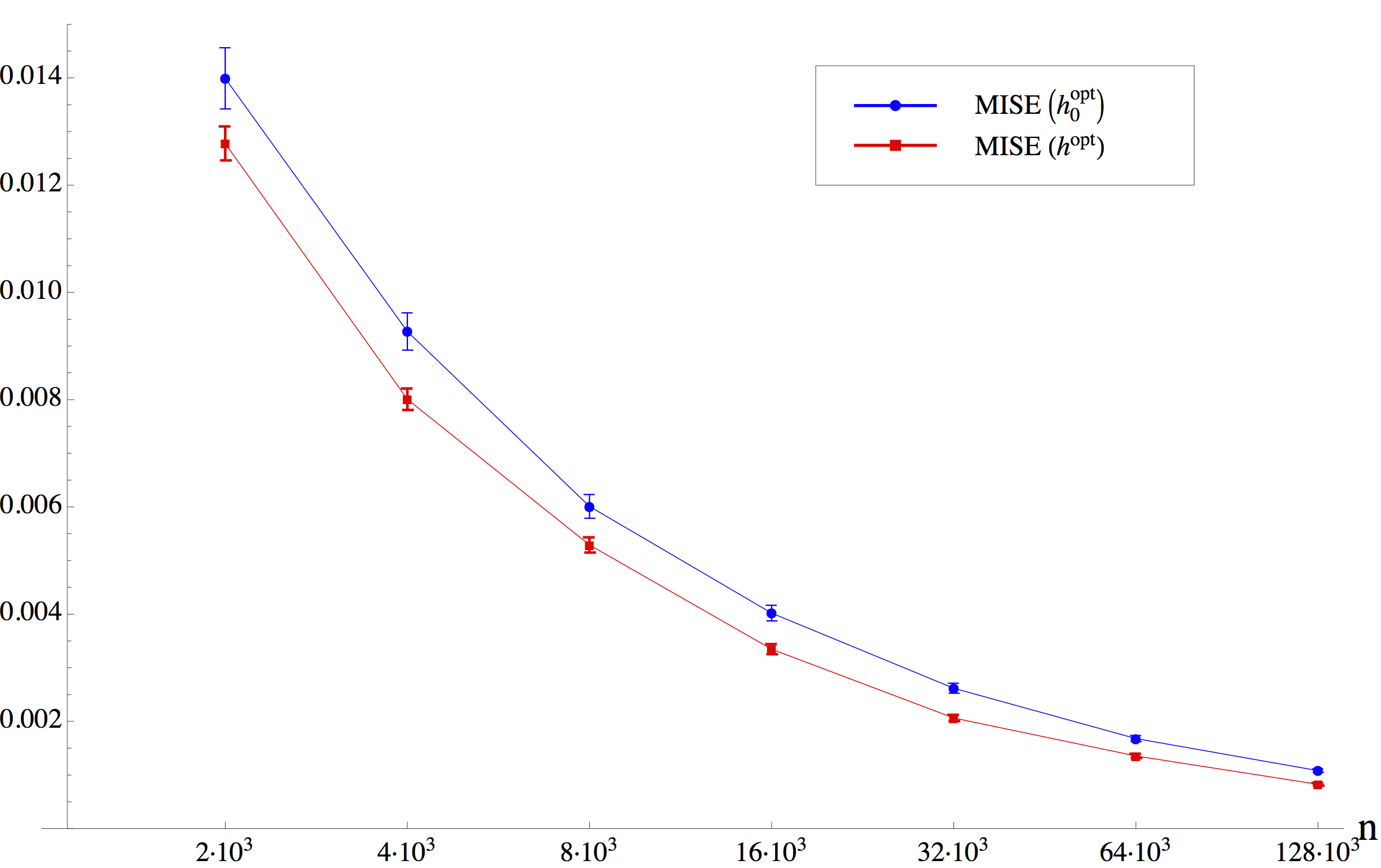
The experiments we ran allow us to compare the behavior of MISE​[p​(x),p^​(x),𝐡]\mbox{\rm MISE}[p(x),\widehat{p}(x),\mathbf{h}] when we select 𝐡=𝐡0opt\mathbf{h}={\bf h}^{\rm opt}_{0} from (5.6) and when we select 𝐡=𝐡opt\mathbf{h}={\bf h}^{\rm opt} from (5.4). Figures 1(a) and 1(b) demonstrate that the latter choice is clearly a superior one.
Refer to caption
(a) M=4M=4

Refer to caption
(b) M=8M=8
Figure 1: MISE​[p,p^,𝐍​(n),𝐡]\mbox{\rm MISE}[p,\widehat{p},\mathbf{N}(n),\mathbf{h}] for 𝐡opt{\bf h}^{\rm opt} and 𝐡0opt{\bf h}^{\rm opt}_{0}.

The rate of decay of the error is very close to O(∥𝐍∥−4/5)O(\|\mathbf{N}\|^{-4/5}), which is consistent with our calculations.

It must be noted, that the graphs are plotted at the theoretically optimal values of 𝐡\mathbf{h}, and the question of whether or not the error can be improved, must be addressed. Our experiment computes the values of MISE for a variety of values of 𝐡\mathbf{h} and the bandwidth that produces the smallest error is indeed slightly different from our theoretical predictions. However, the discrepancy between them is negligible and it does become smaller as sample sizes increase.

Let us define

𝐡MISEopt\displaystyle{\bf h}^{\rm opt}_{\mbox{\rm MISE}} =argmin𝐡∈ℝ+M​MISE​[p∗,p^∗;𝐍,𝐡]\displaystyle=\mathrm{argmin}_{\mathbf{h}\in\mathbb{R}^{M}_{+}}\mbox{\rm MISE}[p^{*},\widehat{p}^{*};\mathbf{N},\mathbf{h}]
=argminh∈ℝ+​MISE​[p∗,p^∗;𝐍,(h,h,…,h)],\displaystyle=\mathrm{argmin}_{h\in\mathbb{R}_{+}}\mbox{\rm MISE}[p^{*},\widehat{p}^{*};\mathbf{N},(h,h,\ldots,h)],
=hMISEopt⋅(1,1,…,1)\displaystyle=h^{\mathrm{opt}}_{\mbox{\rm MISE}}\cdot(1,1,\ldots,1)

where the last two equalities hold in view of the symmetry assumption on p∗p^{*}.

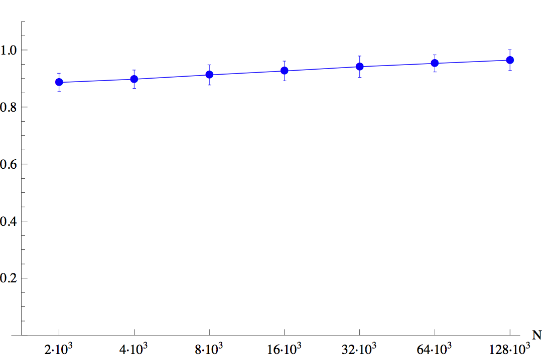
Figure 2 shows that the ratio of the numerically computed approximation of 𝐡MISEopt{\bf h}^{\rm opt}_{\mbox{\rm MISE}} to the theoretically predicted value 𝐡opt{\bf h}^{\rm opt} stays very close to one, which confirms validity of our approach.
Refer to caption
(a) M=4M=4

Refer to caption
(b) M=8M=8
Figure 2: The ratio hopt/hMISEopth^{\mathrm{opt}}/h^{\mathrm{opt}}_{\mbox{\rm MISE}}for different subset configurations.

5.5 Numerical experiments with gamma distributed subset posterior densities

5.5.1 Description of the experiment

The numerical experiment mimics the one with normally distributed samples, with the only difference that this experiment generates samples distributed with Γ⁡(x,α=3,β=3)\Gamma(x,\alpha=3,\beta=3).

5.5.2 Numerical results

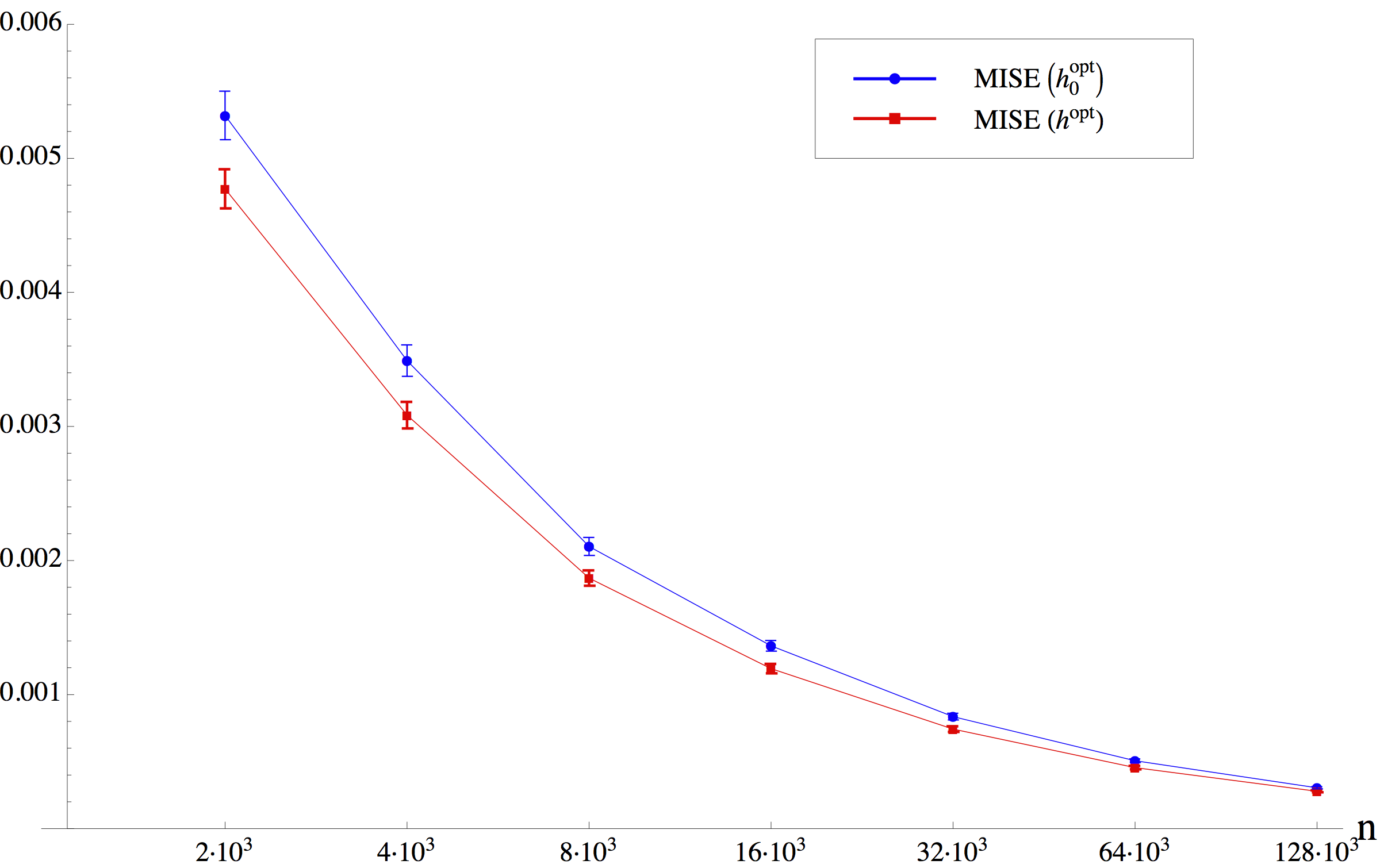
The results of the experiments replicate the same behavior for gamma distributed samples. We must note that the location of the optimal bandwidth parameter is significantly different that in the case of normally distributed samples. Nevertheless, the results are clearly show the advantage of our choice of 𝐡\mathbf{h}, which is demonstrated in Figures 3(a) and 3(b).

Refer to caption
(a) M=4M=4

Refer to caption
(b) M=8M=8
Figure 3: MISE​[p,p^,𝐍​(n),𝐡]\mbox{\rm MISE}[p,\widehat{p},\mathbf{N}(n),\mathbf{h}] for 𝐡opt{\bf h}^{\rm opt} and 𝐡0opt{\bf h}^{\rm opt}_{0}.

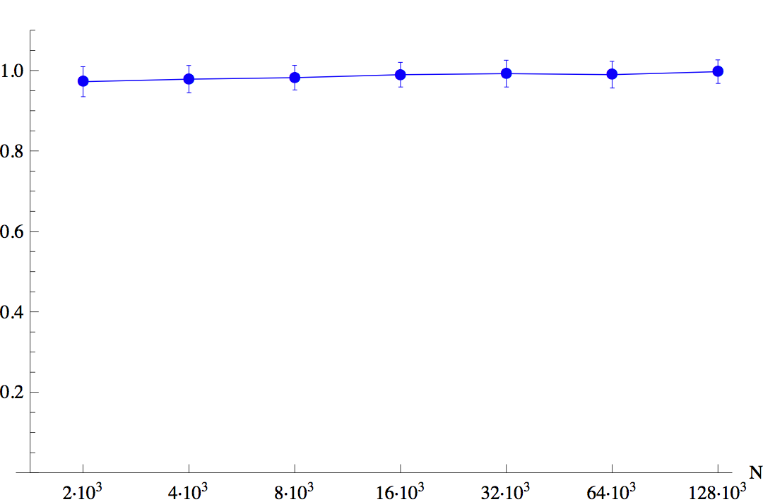
Just as before, our experiment verify that formula (5.7) yields near optimum values of MISE, see Figure 4.

Refer to caption
(a) M=4M=4

Refer to caption
(b) M=8M=8
Figure 4: The ratio of hopt/hMISEopth^{\mathrm{opt}}/h^{\mathrm{opt}}_{\mbox{\rm MISE}}for different subset configurations.

6 Appendix

6.1 Kernel density estimators and asymptotic error analysis

In this section we will use the following notation. The function ff denotes a probability density and its kernel density estimator is given by

f^​(x,X1,X2,…,XN,h)=1N​h​∑i=1NK⁡(x−Xih).\hat{f}(x;X_{1},X_{2},\dots,X_{N},h)=\frac{1}{Nh}\sum_{i=1}^{N}K\left(\frac{x-X_{i}}{h}\right). (6.1)

where X1,X2,…​Xn∼fX_{1},X_{2},\dots X_{n}\sim f are i.i.d. samples.

Lemma 6.1 (bias expansion).

Let KK satisfy (H3) and (H4). Let ff be a probability density function satisfying (H5) and (H6). Let f^n,h​(x)\widehat{f}_{n,h}(x) be an estimation of ff given by (6.1). Then

  • (i)(i)

    bias​(f^n,h)\text{\rm bias}(\widehat{f}_{n,h}) is given by

    [\displaystyle\big[ bias(f^n,h)](x)=\displaystyle\text{\rm bias}(\widehat{f}_{n,h})\big](x)= (6.2)
    =𝔼⁡[f^n,h​(x)]−f⁡(x)=h2​k2​f′′​(x)2+[Eb​(f,K)]​(x,h)\displaystyle=\mathbb{E}\big[\widehat{f}_{n,h}(x)\big]-f(x)=\frac{h^{2}k_{2}f^{\prime\prime}(x)}{2}+{[E_{b}(f,K)](x\hskip 1.0pt;h)}

    where

    Eb​(x,h):=∫ℝK⁡(t)​(∫xx−h​tf′′′​(z)​(x−h​t−z)22​𝑑z)​𝑑t.E_{b}(x;h):=\int_{\mathbb{R}}K(t)\Big(\int_{x}^{x-ht}\frac{f^{\prime\prime\prime}(z)(x-ht-z)^{2}}{2}\,dz\Big)\,dt\,. (6.3)
  • (i​i)(ii)

    For all n≥1n\geq 1 and h>0h>0 the term Eb​(⋅,n,h)E_{b}(\cdot\hskip 1.0pt;n,h) satisfies the bounds

    |Eb​(x,h)|≤C​k36​h3,x∈ℝ\displaystyle|E_{b}(x\hskip 1.0pt;h)|\,\leq\,\frac{Ck_{3}}{6}h^{3}\,,\quad x\in\mathbb{R} (6.4)
    ∫ℝ\displaystyle\int_{\mathbb{R}} |Eb​(x,h)|​d​x≤C​k36​h3\displaystyle|E_{b}(x\hskip 1.0pt;h)|\,dx\,\leq C\frac{k_{3}}{6}h^{3}
    ∫ℝ\displaystyle\int_{\mathbb{R}} |Eb​(x,n,h)|2​d​x≤C2​k3236​h6\displaystyle|E_{b}(x\hskip 1.0pt;n,h)|^{2}\,dx\,\leq\,\frac{C^{2}k_{3}^{2}}{36}h^{6}

    for some constant CC.

  • (i​i​i)(iii)

    The square-integrated b​i​a​s​(f^n,k)bias(\widehat{f}_{n,k}) satisfies

    ∫ℝbias2​(f^n,k)​𝑑x=h4​k224​∫ℝ(f′′​(x))2​𝑑x+ℰb​(n,h)<∞\int_{\mathbb{R}}\text{\rm bias}^{2}(\widehat{f}_{n,k})\,dx\,=\,\frac{h^{4}k_{2}^{2}}{4}\int_{\mathbb{R}}(f^{\prime\prime}(x))^{2}\,dx+\mathcal{E}_{b}(n,h)\,<\,\infty (6.5)

    with

    |ℰb​(n,h)|≤Cb​(k2+k36​h)​k3​h56|\mathcal{E}_{b}(n,h)|\leq C_{b}\Big(k_{2}+\frac{k_{3}}{6}h\Big)\frac{k_{3}h^{5}}{6} (6.6)

    for some constant CbC_{b}, and all n≥1n\geq 1, h>0h>0.

Proof.

Using (6.1) and the fact that XiX_{i}, i=1,…,ni=1,\dots,n are i.i.d. we obtain

biasn,h​(x)\displaystyle\text{\rm bias}_{n,h}(x) =𝔼⁡[f^n,h​(x)]−f⁡(x)=\displaystyle=\mathbb{E}\big[\widehat{f}_{n,h}(x)\big]-f(x)=
=1h​𝔼​[K⁡(x−X1h)]−f⁡(x)\displaystyle=\frac{1}{h}\mathbb{E}\Big[K\Big(\frac{x-X_{1}}{h}\Big)\Big]-f(x)
=1h​∫ℝK⁡(x−yh)​f​(y)​dy−f⁡(x)\displaystyle=\frac{1}{h}\int_{\mathbb{R}}K\Big(\frac{x-y}{h}\Big)f(y)\,dy-f(x)
=∫ℝK⁡(t)​(f⁡(x−h​t)−f⁡(x))​𝑑t\displaystyle=\int_{\mathbb{R}}K(t)\big(f(x-ht)-f(x)\big)\,dt

where we used the substitution t=(x−y)/ht=(x-y)/h. Employing Taylor’s Theorem with an error term in integral form and using (H3) we get

biasn,h​(x)\displaystyle\text{\rm bias}_{n,h}(x) =∫ℝK⁡(t)​(−h​t​f′​(x)+h2​t22​f′′​(x)+∫xx−h​tf′′′​(z)​(x−h​t−z)22​𝑑z)​𝑑t\displaystyle=\int_{\mathbb{R}}K(t)\bigg(-htf^{\prime}(x)+\frac{h^{2}t^{2}}{2}f^{\prime\prime}(x)+\int_{x}^{x-ht}\frac{f^{\prime\prime\prime}(z)(x-ht-z)^{2}}{2}\,dz\bigg)\,dt
=h2​f′′​(x)2​∫ℝt2​K​(t)​𝑑t+∫ℝK⁡(t)​(∫xx−h​tf′′′​(z)​(x−h​t−z)22​𝑑z)​𝑑t\displaystyle=\frac{h^{2}f^{\prime\prime}(x)}{2}\int_{\mathbb{R}}t^{2}K(t)\,dt+\int_{\mathbb{R}}K(t)\Big(\int_{x}^{x-ht}\frac{f^{\prime\prime\prime}(z)(x-ht-z)^{2}}{2}\,dz\Big)\,dt

which proves (i)(i).

By (H4) we have

|Eb​(x,n,h)|⩽C⁡(∫ℝK⁡(t)​|∫xx−h​t(x−h​t−z)22​𝑑z|​𝑑t)=C​k36​h3|E_{b}(x\hskip 1.0pt;n,h)|\leqslant C\bigg(\int_{\mathbb{R}}K(t)\bigg|\int_{x}^{x-ht}\frac{(x-ht-z)^{2}}{2}\,dz\bigg|\,dt\bigg)=\frac{Ck_{3}}{6}h^{3} (6.7)

and by (H6), using the substitution α=x−h​t−z\alpha=x-ht-z and employing Tonelli’s Theorem, we obtain

∫ℝ|Eb\displaystyle\int_{\mathbb{R}}|E_{b} (x,n,h)|d​x\displaystyle(x\hskip 1.0pt;n,h)|\,dx (6.8)
≤∫ℝ∫ℝK⁡(t)​∫x−h2​(|t|+t)x+h2​(|t|−t)|f′′′​(z)|​(x−h​t−z)22​𝑑z​𝑑t​𝑑x\displaystyle\leq\,\int_{\mathbb{R}}\int_{\mathbb{R}}K(t)\int_{x-\frac{h}{2}(|t|+t)}^{x+\frac{h}{2}(|t|-t)}\frac{|f^{\prime\prime\prime}(z)|(x-ht-z)^{2}}{2}\,dz\,dt\,dx
=∫ℝK⁡(t)​∫−h2​(|t|+t)h2​(|t|−t)((∫ℝ|f′′′​(x−h​t−α)|​𝑑x)​α22)​𝑑α​𝑑t\displaystyle=\,\int_{\mathbb{R}}K(t)\int_{-\frac{h}{2}(|t|+t)}^{\frac{h}{2}(|t|-t)}\bigg(\Big(\int_{\mathbb{R}}|f^{\prime\prime\prime}(x-ht-\alpha)|\,dx\Big)\frac{\alpha^{2}}{2}\bigg)\,d\alpha\,dt
≤C​∫ℝK⁡(t)​(∫−h2​(|t|−t)h2​(|t|+t)α22​dα)​dt=h36​C​k3.\displaystyle\leq\,C\int_{\mathbb{R}}K(t)\bigg(\int_{-\frac{h}{2}(|t|-t)}^{\frac{h}{2}(|t|+t)}\frac{\alpha^{2}}{2}\,d\alpha\,\bigg)dt=\frac{h^{3}}{6}Ck_{3}\,.

Thus, combining the two bounds above we conclude

∫ℝ|Eb​(x,n,h)|2​𝑑x≤C​k36​h3​∫ℝ|Eb​(x,n,h)|​𝑑x≤C2​k3236​h6.\int_{\mathbb{R}}|E_{b}(x\hskip 1.0pt;n,h)|^{2}\,dx\leq\frac{Ck_{3}}{6}h^{3}\int_{\mathbb{R}}|E_{b}(x\hskip 1.0pt;n,h)|\,dx\leq\frac{C^{2}k_{3}^{2}}{36}h^{6}\,.

Observe that

bias2​(f^n,h)​(x)=h4​k224​(f′′​(x))2+h2​k2​f′′​(x)​Eb​(x,n,h)+Eb2​(x,n,h).\displaystyle\text{\rm bias}^{2}(\widehat{f}_{n,h})(x)=\frac{h^{4}k_{2}^{2}}{4}(f^{\prime\prime}(x))^{2}+h^{2}k_{2}f^{\prime\prime}(x)E_{b}(x\hskip 1.0pt;n,h)+E_{b}^{2}(x;n,h)\,. (6.9)

By (H5), (6.7) and (6.8)

|ℰb​(n,h)|\displaystyle\big|\mathcal{E}_{b}(n,h)\big| :=|∫ℝ(h2​k2​f′′​(x)​Eb​(x,n,h)+Eb2​(x,n,h))​𝑑x|\displaystyle:=\bigg|\int_{\mathbb{R}}\Big(h^{2}k_{2}f^{\prime\prime}(x)E_{b}(x\hskip 1.0pt;n,h)+E_{b}^{2}(x;n,h)\Big)\,dx\bigg| (6.10)
≤(h2​k2​C+C​k36​h3)​∫ℝ|Eb​(x,n,h)|\displaystyle\leq\Big(h^{2}k_{2}C+\frac{Ck_{3}}{6}h^{3}\Big)\int_{\mathbb{R}}|E_{b}(x\hskip 1.0pt;n,h)|
≤(h2​k2​C+C​k36​h3)​h36​C​k3.\displaystyle\leq\Big(h^{2}k_{2}C+\frac{Ck_{3}}{6}h^{3}\Big)\frac{h^{3}}{6}Ck_{3}\,.

By (H5) and (H6) we have ∫ℝ(f′′​(x))2​𝑑x<∞\int_{\mathbb{R}}(f^{\prime\prime}(x))^{2}\,dx<\infty. Hence by setting Cb=C2C_{b}=C^{2}, using (6.9) and (6.10) we obtain (6.6). ∎

Lemma 6.2 (variation expansion).

Let KK satisfy (H3) and (H4), with r=2r=2. Let ff satisfy (H5) and (H6), and f^n,h​(x)\widehat{f}_{n,h}(x) be the estimator of ff given by (6.1). Then

  • (i)(i)

    𝕍⁡(f^n,h)\mathbb{V}(\widehat{f}_{n,h}) is given by

    [𝕍⁡(f^n,h)]​(x)=f⁡(x)​1n​h​∫ℝK2​(t)​𝑑t+EV​(x,n,h),x∈ℝ\big[\mathbb{V}(\widehat{f}_{n,h})\big](x)=f(x)\frac{1}{nh}\int_{\mathbb{R}}K^{2}(t)\,dt+E_{V}(x\hskip 1.0pt;n,h)\,,\quad x\in\mathbb{R} (6.11)

    with

    EV​(x,n,h)\displaystyle E_{V}(x;n,h) =−1n​(∫ℝt​K2​(t)​∫01f′​(x−h​t​u)​du​dt+(f⁡(x)+bias​(f^n,h)​(x))2)\displaystyle=-\frac{1}{n}\bigg(\int_{\mathbb{R}}tK^{2}(t)\int_{0}^{1}\hskip 1.0ptf^{\prime}(x-htu)\,du\,dt+\Big(f(x)+\text{\rm bias}(\widehat{f}_{n,h})(x)\Big)^{2}\bigg)\, (6.12)
  • (ii)

    The term EV​(x,n,h)E_{V}(x\hskip 1.0pt;n,h) satisfies

    ℰV​(n,h)\displaystyle\mathcal{E}_{V}(n,h) =|∫ℝEV​(x)​dx|\displaystyle=\left|\int_{\mathbb{R}}E_{V}(x)\,dx\right| (6.13)
    ≤CVn​(2+h2​k2+(k2+k33​h)​h56​k3).\displaystyle\leq\hskip 1.0pt\frac{C_{V}}{n}\bigg(2+h^{2}k_{2}+\big(k_{2}+\frac{k_{3}}{3}h\big)\frac{h^{5}}{6}k_{3}\Big)\,.
Proof.

Using (6.2) and the fact that XiX_{i}, i=1,…,ni=1,\dots,n, are i.i.d. we obtain

𝕍​(f^n,h​(x))\displaystyle\mathbb{V}(\widehat{f}_{n,h}(x)) =𝕍⁡(1h​K​(x−X1h))\displaystyle=\mathbb{V}\Big(\frac{1}{h}K\Big(\frac{x-X_{1}}{h}\Big)\Big)
=1n​∫ℝ1h2​K2​(x−yh)​f​(y)​dy−1n​(∫ℝ1h​K​(x−yh)​f​(y)​dy)2\displaystyle=\frac{1}{n}\int_{\mathbb{R}}\frac{1}{h^{2}}K^{2}\left(\frac{x-y}{h}\right)f(y)\,dy-\frac{1}{n}\left(\int_{\mathbb{R}}\frac{1}{h}K\left(\frac{x-y}{h}\right)f(y)\,dy\right)^{2}
=1n​h​∫ℝK2​(t)​f​(x−h​t)​dt−1n​(f⁡(x)+bias​(f^n,h)​(x))2\displaystyle=\frac{1}{nh}\int_{\mathbb{R}}K^{2}(t)f(x-ht)\,dt-\frac{1}{n}\Big(f(x)+\text{\rm bias}(\widehat{f}_{n,h})(x)\Big)^{2}
=1n​h​∫ℝK2​(t)​f​(x)​𝑑t+1n​h​∫ℝK2​(t)​(∫xx−h​tf′​(z)​𝑑z)​𝑑t\displaystyle=\frac{1}{nh}\int_{\mathbb{R}}K^{2}(t)f(x)\,dt+\frac{1}{nh}\int_{\mathbb{R}}K^{2}(t)\Big(\int_{x}^{x-ht}f^{\prime}(z)\,dz\,\Big)dt
−1n​(f⁡(x)+bias​(f^n,h)​(x))2\displaystyle-\frac{1}{n}\Big(f(x)+\text{\rm bias}(\widehat{f}_{n,h})(x)\Big)^{2}
=1n​h​∫ℝK2​(t)​f​(x)​𝑑t−1n​∫ℝt​K2​(t)​∫01f′​(x−h​t​u)​𝑑u​𝑑t\displaystyle=\frac{1}{nh}\int_{\mathbb{R}}K^{2}(t)f(x)\,dt-\frac{1}{n}\int_{\mathbb{R}}tK^{2}(t)\int_{0}^{1}f^{\prime}(x-htu)\,du\,dt
−1n​(f⁡(x)+bias​(f^n,h)​(x))2\displaystyle-\frac{1}{n}\Big(f(x)+\text{\rm bias}(\widehat{f}_{n,h})(x)\Big)^{2}

which proves (6.11) and (6.12).

We next estimate the terms

E1(x):=∫ℝtK2(t)(∫01f′(x−htu)du)dt,E2(x):=(f(x)+bias(f^n,h)(x))2.\displaystyle E_{1}(x):=\int_{\mathbb{R}}tK^{2}(t)\bigg(\int_{0}^{1}f^{\prime}(x-htu)\,du\bigg)\,dt\,,\quad E_{2}(x):=\Big(f(x)+\text{\rm bias}(\widehat{f}_{n,h})(x)\Big)^{2}\,.

Observe that (H5)-(H6) imply

∫ℝ|f′​(x)|​𝑑x=∫ℝ|f′​(x+α)|​𝑑x:=I1<∞\int_{\mathbb{R}}|f^{\prime}(x)|\,dx=\int_{\mathbb{R}}|f^{\prime}(x+\alpha)|\,dx:=I_{1}\,<\,\infty

for any α∈ℝ\alpha\in\mathbb{R}. Then using Tonelli’s Theorem ans (H4) we obtain

∫ℝ|E1​(x)|​𝑑x\displaystyle\int_{\mathbb{R}}|E_{1}(x)|\,dx ≤∫ℝ|t|​K2​(t)​(∫ℝ∫01|f′​(x−h​t​u)|​𝑑u​𝑑x)​𝑑t\displaystyle\leq\int_{\mathbb{R}}|t|K^{2}(t)\bigg(\int_{\mathbb{R}}\int_{0}^{1}|f^{\prime}(x-htu)|\,du\,dx\bigg)\,dt
≤∫ℝ|t|​K2​(t)​(∫01(∫ℝ|f′​(x−h​t​u)|​dx)​du)​dt≤I1​k1\displaystyle\leq\int_{\mathbb{R}}|t|K^{2}(t)\bigg(\int_{0}^{1}\Big(\int_{\mathbb{R}}|f^{\prime}(x-htu)|\,dx\Big)\,du\bigg)\,dt\leq I_{1}k_{1}

Since E1E_{1} is integrable we can use Fubini’s Theorem and this yields

∫ℝE1​(x)​𝑑x\displaystyle\int_{\mathbb{R}}E_{1}(x)\,dx =∫ℝt​K2​(t)​(∫ℝ∫01f′​(x−h​t​u)​𝑑u​𝑑x)​𝑑t\displaystyle=\int_{\mathbb{R}}tK^{2}(t)\bigg(\int_{\mathbb{R}}\int_{0}^{1}f^{\prime}(x-htu)\,du\,dx\bigg)\,dt
=∫ℝt​K2​(t)​(∫01(∫ℝf′​(x−h​t​u)​dx)​du)​dt=0\displaystyle=\int_{\mathbb{R}}tK^{2}(t)\bigg(\int_{0}^{1}\Big(\int_{\mathbb{R}}f^{\prime}(x-htu)\,dx\Big)\,du\bigg)\,dt=0

where we used the fact that limx→±∞f⁡(x)=0\lim_{x\to\pm\infty}f(x)=0. Next, by (H5) and (6.4) we get

∫ℝ|E2​(x)|​𝑑x\displaystyle\int_{\mathbb{R}}|E_{2}(x)|\,dx ≤2​∫ℝ(f2​(x)+bias2​(f^n,h)​(x))​𝑑x\displaystyle\leq 2\int_{\mathbb{R}}\Big(f^{2}(x)+\text{\rm bias}^{2}(\widehat{f}_{n,h})(x)\Big)\,dx
≤2​C+C​h2​k2+(k2​C+C​k36​h)​h53​C​k3.\displaystyle\leq 2C+Ch^{2}k_{2}+\Big(k_{2}C+\frac{Ck_{3}}{6}h\Big)\frac{h^{5}}{3}Ck_{3}\,.

Combining the above estimates we obtain (6.13) . ∎

Lemma 6.3 (kernel autocorrelation).

Let KK satisfy (H3) and (H4), then the function

K2​(z)=∫ℝK⁡(s)​K​(s−z)​𝑑s≥0,z∈ℝK_{2}(z)=\int_{\mathbb{R}}K(s)K(s-z)\,ds\geq 0\,,\quad z\in\mathbb{R}

satisfies

∫ℝK2​(z)​𝑑z\displaystyle\int_{\mathbb{R}}K_{2}(z)\,dz =1,∫ℝz​K2​(z)​𝑑z\displaystyle=1,\quad\int_{\mathbb{R}}z\,K_{2}(z)\,dz =0.\displaystyle=0\,.

Moreover, for any sufficiently smooth f⁡(x)f(x)

∫1h​K2​(z−xh)​f​(z)​𝑑z=f⁡(x)+EC,fwith|EC,f|≤‖f′′‖∞​k2​h2.\int\frac{1}{h}K_{2}\left(\frac{z-x}{h}\right)f(z)\,dz=f(x)+E_{C,f}\quad\text{with}\quad|E_{C,f}|\leq\|f^{\prime\prime}\|_{\infty}k_{2}h^{2}\,.
Proof.

Since K≥0K\geq 0 we have K2≥0K_{2}\geq 0. Moreover, we have

∫ℝK2​(z)​𝑑z=∬ℝ×ℝK⁡(s)​K​(s−z)​𝑑z​𝑑s=1\int_{\mathbb{R}}K_{2}(z)\,dz=\iint_{\mathbb{R}\times\mathbb{R}}K(s)K(s-z)\,dzds=1

and this proves the first property. Similarly, recalling that ∫z​K​(z)​𝑑z=0\int zK(z)\,dz=0, we obtain

∫ℝz​K2​(z)​𝑑z\displaystyle\int_{\mathbb{R}}z\,K_{2}(z)\,dz =∫ℝK⁡(s)​∫ℝ(z−s+s)​K​(s−z)​dz​ds=0.\displaystyle=\int_{\mathbb{R}}K(s)\int_{\mathbb{R}}(z-s+s)K(s-z)\,dz\,ds=0\,.

Next, we take any smooth function ff and compute

∫1h​K2​(z−xh)​f​(z)​𝑑z=∫K2​(u)​f​(x−h​u)​𝑑u\displaystyle\int\frac{1}{h}K_{2}\left(\frac{z-x}{h}\right)f(z)\,dz=\int K_{2}\left(u\right)f(x-hu)\,du
=f⁡(x)+∫K2​(u)​∫xx−h​uf′′​(t)​(t−x+h​u)​dt​du.\displaystyle=f(x)+\int K_{2}(u)\int_{x}^{x-hu}f^{\prime\prime}(t)(t-x+hu)\,dt\,du\,.

Finally, we estimate the last term in the above formula as follows

|∫K2​(u)​∫xx−h​uf′′​(t)​(t−x+h​u)​dt​du|\displaystyle\left|\int K_{2}(u)\int_{x}^{x-hu}f^{\prime\prime}(t)(t-x+hu)\,dt\,du\right|
≤‖f′′‖∞​∫K2​(u)​h2​u22​𝑑u\displaystyle\leq\|f^{\prime\prime}\|_{\infty}\int K_{2}(u)\frac{h^{2}u^{2}}{2}\,du
=‖f′′‖∞​h22​(∫K⁡(s)​∫(s−u)2​K​(s−u)​du​ds+∫s2​K​(s)​∫K⁡(s−u)​du​ds)\displaystyle=\frac{\|f^{\prime\prime}\|_{\infty}h^{2}}{2}\left(\int K(s)\int(s-u)^{2}K(s-u)\,duds+\int s^{2}K(s)\int K(s-u)\,duds\right)
≤‖f′′‖∞​k2​h2.\displaystyle\leq\|f^{\prime\prime}\|_{\infty}k_{2}h^{2}\,.

∎

Lemma 6.4 (product expectation).

Let KK satisfy (H3) and (H4), with r=2r=2. Let ff be a probability density function that satisfies (H5) and (H6), and let f^n,h​(x)\widehat{f}_{n,h}(x) be an estimate of ff given by (6.1). Then

𝔼⁡[f^n,h​(x)​f^n,h​(y)]−𝔼⁡[f^n,h​(x)]​𝔼​[f^n,h​(y)]=1N​h​f​(x)​K2​(x−yh)−EΠ,\mathbb{E}[\widehat{f}_{n,h}(x)\widehat{f}_{n,h}(y)]-\mathbb{E}[\widehat{f}_{n,h}(x)]\mathbb{E}[\widehat{f}_{n,h}(y)]=\frac{1}{Nh}f(x)K_{2}\Big(\frac{x-y}{h}\Big)-E_{\Pi}, (6.14)

where the error term

EΠ=1N​∫(s​K​(s)​K​(s−x−yh)​(∫01f′​(x−s​h​u)​𝑑u))​𝑑s+1N​𝔼​[f^​(x)]​𝔼​[f^​(y)]E_{\Pi}=\frac{1}{N}\int\bigg(\,sK(s)K\big(s-\frac{x-y}{h}\big)\Big(\int_{0}^{1}f^{\prime}(x-shu)\,du\big)\bigg)ds+\frac{1}{N}\mathbb{E}[\widehat{f}(x)]\mathbb{E}[\widehat{f}(y)]

satisfies

|EΠ​(x,y)|≤CΠN,|∫∫⁡EΠ​(x,y)​dx​dy|≤1N​(1+C​k3​h36)2\displaystyle|E_{\Pi}(x,y)|\leq\frac{C_{\Pi}}{N}\,,\qquad\Big|\int\int E_{\Pi}(x,y)\,dxdy\Big|\leq\frac{1}{N}\left(1+\frac{Ck_{3}h^{3}}{6}\right)^{2} (6.15)
∫∫⁡|EΠ​(x,y)|​dx​dy≤1N​(1+k1​C​C​k2​h22+C​k3​h36)2\displaystyle\int\int\Big|E_{\Pi}(x,y)\Big|dxdy\leq\frac{1}{N}\left(1+k_{1}\,C\frac{Ck_{2}h^{2}}{2}+\frac{Ck_{3}h^{3}}{6}\right)^{2}

for some constant CΠC_{\Pi} and constants CC given in (H6) and K2K_{2} defined in Lemma 6.3.

Proof.

By the definition of the estimator f^\widehat{f} we have

𝔼​(f^​(x)​f^​(y))\displaystyle\mathbb{E}\Big(\widehat{f}(x)\widehat{f}(y)\bigg) =𝔼⁡(1N2​h2​∑i,j=1NK⁡(x−Xih)​K​(y−Xjh)).\displaystyle=\mathbb{E}\bigg(\frac{1}{N^{2}h^{2}}\sum_{i,j=1}^{N}K\Big(\frac{x-X_{i}}{h}\Big)K\Big(\frac{y-X_{j}}{h}\Big)\bigg)\,. (6.16)

Since all {Xi}i=1N\{X_{i}\}_{i=1}^{N} are i.i.d. we can split the calculation into two parts, one for the part, where the indexes coincide and the part, where indexes are different. We then can use the independence of the samples to simplify the calculation

𝔼​(f^​(x)​f^​(y))\displaystyle\mathbb{E}\Big(\widehat{f}(x)\widehat{f}(y)\bigg) =1N2​h2​𝔼​(∑i=jK⁡(x−Xih)​K​(y−Xih))\displaystyle=\frac{1}{N^{2}h^{2}}\mathbb{E}\bigg(\sum_{i=j}K(\frac{x-X_{i}}{h})K(\frac{y-X_{i}}{h})\bigg) (6.17)
+1N2​h2​𝔼​(∑i≠jK⁡(x−Xih)​K​(y−Xjh))\displaystyle+\frac{1}{N^{2}h^{2}}\mathbb{E}\bigg(\sum_{i\neq j}K\Big(\frac{x-X_{i}}{h}\Big)K\Big(\frac{y-X_{j}}{h}\Big)\bigg)
=1N​h2​[𝔼⁡(K⁡(x−Xh)​K​(y−Xh))]+(1−1N)​𝔼​[f^​(x)]​𝔼​[f^​(y)]\displaystyle{\displaystyle=\frac{1}{Nh^{2}}\left[\mathbb{E}\Big(K\Big(\frac{x-X}{h}\Big)K\Big(\frac{y-X}{h}\Big)\bigg)\right]+\Big(1-\frac{1}{N}\Big)\mathbb{E}[\widehat{f}(x)]\mathbb{E}[\widehat{f}(y)]}

where X=X1X=X_{1}. The first expectation term in (6.17) can be expanded as

1N​h2​𝔼​[K⁡(x−Xh)​K​(y−Xh)]\displaystyle\frac{1}{Nh^{2}}\mathbb{E}\left[K\left(\frac{x-X}{h}\right)K\left(\frac{y-X}{h}\right)\right]
=1N​h2​∫K⁡(x−th)​K​(y−th)​f​(t)​𝑑t\displaystyle=\frac{1}{Nh^{2}}\int\,K\Big(\frac{x-t}{h}\Big)K\Big(\frac{y-t}{h}\Big)\,f(t)\,dt
=1N​h​∫K⁡(s)​K​(s−x−yh)​(f⁡(x)+∫xx−s​hf′​(z)​𝑑z)​𝑑s\displaystyle=\frac{1}{Nh}\int\,K(s)K\Big(s-\frac{x-y}{h}\Big)\,\Big(f(x)+\int_{x}^{x-sh}f^{\prime}(z)\,dz\Big)\,ds
=f⁡(x)​1N​h​K2​(x−yh)\displaystyle=f(x)\frac{1}{Nh}K_{2}\Big(\frac{x-y}{h}\Big)
−1N∫sK(s)K(s−x−yh)(∫01f′(x−shu)du)ds\displaystyle-\frac{1}{N}\int\,sK(s)K\Big(s-\frac{x-y}{h}\Big)\,\bigg(\int_{0}^{1}f^{\prime}\left(x-shu\right)\,du\bigg)\,ds

Let us denote

EΠ,1=1N​∫(s​K​(s)​K​(s−x−yh)​(∫01f′​(x−s​h​u)​𝑑u))​𝑑s,EΠ,2=1N​𝔼​[f^​(x)]​𝔼​[f^​(y)].E_{\Pi,1}=\frac{1}{N}\int\bigg(\,sK(s)K\big(s-\frac{x-y}{h}\big)\Big(\int_{0}^{1}f^{\prime}(x-shu)\,du\big)\bigg)ds\,,\quad E_{\Pi,2}=\frac{1}{N}\mathbb{E}[\widehat{f}(x)]\mathbb{E}[\widehat{f}(y)].

Then we obtain

𝔼⁡(f^n,h​(x)​f^n,h​(y))−𝔼⁡[f^n,h​(x)]​𝔼​[f^n,h​(y)]\displaystyle\mathbb{E}\Big(\widehat{f}_{n,h}(x)\widehat{f}_{n,h}(y)\bigg)-\mathbb{E}[\widehat{f}_{n,h}(x)]\mathbb{E}[\widehat{f}_{n,h}(y)]
=f⁡(x)​1N​h​K2​(x−yh)​d​s−(EΠ,1+EΠ,2).\displaystyle=f(x)\frac{1}{Nh}K_{2}\Big(\frac{x-y}{h}\Big)ds-(E_{\Pi,1}+E_{\Pi,2}).

and this establishes (6.14).

Observe that (H3), (H4) and (H5) imply

|EΠ,1|≤C​k1N.|E_{\Pi,1}|\leq\frac{C\,k_{1}}{N}\,.

Next, according to (6.2) and (6.4)

|𝔼⁡[f^​(x)]|≤C+C​k2​h22+C​k3​h36for allx∈ℝ|\mathbb{E}[\widehat{f}(x)]|\leq C+\frac{Ck_{2}h^{2}}{2}+\frac{Ck_{3}h^{3}}{6}\quad\text{for all}\quad x\in\mathbb{R}

where CC is a maximum of constants from (H5) and hence

|EΠ,2|≤1N​(C+C​k2​h22+C​k3​h36)2.|E_{\Pi,2}|\leq\frac{1}{N}\Big(C+\frac{Ck_{2}h^{2}}{2}+\frac{Ck_{3}h^{3}}{6}\Big)^{2}\,.

Combining the above estimate we conclude that

|EΠ|=|EΠ,1+EΠ,2|≤1N​(C​k1+(C+C​k2​h22+C​k3​h36)2).|E_{\Pi}|=|E_{\Pi,1}+E_{\Pi,2}|\leq\frac{1}{N}\left(Ck_{1}+\left(C+\frac{Ck_{2}h^{2}}{2}+\frac{Ck_{3}h^{3}}{6}\right)^{2}\right).

To obtain bounds on the integral of the error term, let us consider each component of the error separately. The term EΠ,1E_{\Pi,1} is integrable

∬|EΠ,1​(x,y)|​𝑑x​𝑑y\displaystyle\iint|E_{\Pi,1}(x,y)|\,dxdy ≤1N​∭ℝ3|s|​K​(s)​K​(s−x−yh)​(∫01|f′​(x−s​h​u)|​𝑑u)​𝑑s​𝑑x​𝑑y\displaystyle\leq\frac{1}{N}\iiint_{\mathbb{R}^{3}}\,|s|\,K(s)K\Big(s-\frac{x-y}{h}\Big)\,\Big(\int_{0}^{1}|f^{\prime}\left(x-shu\right)|\,du\Big)ds\,dx\,dy (6.18)
≤1N​∫ℝ|s|​K​(s)​(∫01∫ℝ|f′​(x−s​h​u)|​𝑑x​𝑑u)​𝑑s≤k1​CN\displaystyle\leq\frac{1}{N}\int_{\mathbb{R}}\,|s|\,K(s)\,\Big(\int_{0}^{1}\int_{\mathbb{R}}|f^{\prime}\left(x-shu\right)|\,dx\,du\Big)ds\leq\frac{k_{1}\,C}{N}

Next using Fubini Theorem, we obtain

|∬EΠ,1​(x,y)​dx​dy|\displaystyle\left|\iint E_{\Pi,1}(x,y)\,dxdy\right|
≤1N​|∭ℝ3s​K​(s)​K​(s−x−yh)​(∫01f′​(x−s​h​u)​du)​ds​dx​dy|\displaystyle\leq\frac{1}{N}\left|\iiint_{\mathbb{R}^{3}}\,s\,K(s)K\Big(s-\frac{x-y}{h}\Big)\,\Big(\int_{0}^{1}f^{\prime}\left(x-shu\right)\,du\Big)ds\,dx\,dy\right|
=1N​|∫ℝs​K​(s)​(∫01∫ℝf′​(x−s​h​u)​dx​du)​ds|=0.\displaystyle=\frac{1}{N}\left|\int_{\mathbb{R}}\,s\,K(s)\,\Big(\int_{0}^{1}\int_{\mathbb{R}}f^{\prime}\left(x-shu\right)\,dx\,du\Big)\,ds\right|=0\,.

Therefore, using Lemma 6.1, (6.2), (6.4) and the hypothesis (H6) we obtain

|∬ℝ2EΠ​(x,y)​dx​dy|\displaystyle\left|\iint_{\mathbb{R}^{2}}E_{\Pi}(x,y)\,dxdy\right| =1N​|∫ℝ𝔼⁡[f^​(x)]​dx|2≤1N​(1+C​k3​h36)2.\displaystyle=\frac{1}{N}\left|\int_{\mathbb{R}}\mathbb{E}[\widehat{f}(x)]\,dx\right|^{2}\leq\frac{1}{N}\left(1+\frac{Ck_{3}h^{3}}{6}\right)^{2}\,.

Finally, directly from (6.18), (6.2) and (6.4) we obtained

∬ℝ2|EΠ​(x,y)|​𝑑x​𝑑y\displaystyle\iint_{\mathbb{R}^{2}}\left|E_{\Pi}(x,y)\right|\,dxdy ≤∬ℝ2|EΠ,1​(x,y)|​𝑑x​𝑑y+∬ℝ2|EΠ,2​(x,y)|​𝑑x​𝑑y\displaystyle\leq\iint_{\mathbb{R}^{2}}\left|E_{\Pi,1}(x,y)\right|dxdy+\iint_{\mathbb{R}^{2}}\left|E_{\Pi,2}(x,y)\right|dxdy
≤k1​CN+1N​(1+C​k2​h22+C​k3​h36)2\displaystyle\leq\frac{k_{1}\,C}{N}+\frac{1}{N}\left(1+\frac{Ck_{2}h^{2}}{2}+\frac{Ck_{3}h^{3}}{6}\right)^{2}

∎

Theorem 6.5 (MISE expansion).

Let KK satisfy (H3) and (H4), with r=2r=2. Let ff be a probability density function that satisfies (H5) and (H6), and let f^n,h​(x)\widehat{f}_{n,h}(x) be an estimate of ff given by (6.1). Then

MISE​(f^n,h)=h4​k224​∫ℝ(f′′​(x))2​𝑑x+1n​h​f​(x)​∫ℝK2​(t)​𝑑t+ℰb​(n,h)+ℰV​(n,h)\mbox{\rm MISE}(\widehat{f}_{n,h})=\frac{h^{4}k^{2}_{2}}{4}\int_{\mathbb{R}}(f^{\prime\prime}(x))^{2}dx+\frac{1}{nh}f(x)\int_{\mathbb{R}}K^{2}(t)\,dt+\mathcal{E}_{b}(n,h)+\mathcal{E}_{V}(n,h) (6.19)

with ℰb\mathcal{E}_{b} and ℰV\mathcal{E}_{V} defined in (6.10) and (6.13), respectively. Moreover, for every H>0H>0 there exists Cf,K,HC_{f,K,H} such that

|ℰb​(h,n)+ℰV​(h,n)|⩽Cf,K,H​(h5+1n)|\mathcal{E}_{b}(h,n)+\mathcal{E}_{V}(h,n)|\,\leqslant\,C_{f,K,H}\Big(h^{5}+\frac{1}{n}\Big) (6.20)

for all n≥1n\geq 1 and H≥h>0H\geq h>0.

Proof.

It is easy to show (see [27]) that

MISE​(f^n,h)\displaystyle\mbox{\rm MISE}(\widehat{f}_{n,h}) =∫ℝ𝔼​[f^n,h​(x)−f⁡(x)]2​𝑑x\displaystyle=\int_{\mathbb{R}}\mathbb{E}[\widehat{f}_{n,h}(x)-f(x)]^{2}\,dx
=∫ℝ(bias​(f^n,h)​(x))2​dx+∫ℝ𝕍⁡(f^n,h​(x))​dx.\displaystyle=\int_{\mathbb{R}}\big(\text{\rm bias}(\widehat{f}_{n,h})(x)\big)^{2}\,dx\hskip 1.0pt+\int_{\mathbb{R}}\mathbb{V}(\widehat{f}_{n,h}(x))\,dx\,.

and hence the result follows from Lemma 6.1 and Lemma 6.2. ∎

References

  • [2] N. Atkinson, An introduction in Numerical analysis. John Wiley &\& Sons, 1989.
  • [3] D. B. H. Cline and J. D. Hart, Kernel density estimation of densities with doscontinuities or discontinuous derivatives, Statistics (1991), 22-1, 69-84
  • [4] J. E. Chacón, T. Duong, Multivariate plug-in bandwidth selection with unconstrained pilot bandwidth matrices, Test (2010), 19-2, 375–398
  • [5] D. B. H. Cline, Optimal kernel density estimation of densities, Ann. Inst. Statist. Math. (1990), 42-2, 287-303
  • [6] T. Duong, M. L. Hazelton, Cross validation bandwidth matrices for multivariate kernel density estimation, Scandinavian Journal of Statistics (2005).
  • [7] C. van Eeden, Mean integrated squared error of kernel estimators when the density and its derivative are not necessarily continuous, Ann. Inst. Statist. Math. (1985), 37-A, 461-472
  • [8] M. Rosenblatt, Annals of Mathematical Statistics, 27-3, 1956, 832-837
  • [9] V.A. Epanechnikov, Non-parametric estimation of a multivariate probability density, Theory Prob. Appl. 14, 153-158
  • [10] E. Parzen, On estimation of a probability density function and mode, The annals of mathematical statistics, 1065-1076, (1962).
  • [11] B. van Es, On the expansion of the mean integrated squared error of a kernel density estimator, Statistics and Probability Letters (2000), 52, 441-450
  • [12] Z. Huang, A. Gelman, Sampling for Bayesian computation with large datasets, Technical Report, (2005), Columbia University Department of Statistics.
  • [13] K.B. Laskey, J.W. Myers, Population Markov chain Monte Carlo (2003), Machine Learning, 50, 175-196.
  • [14] L.M. Le Cam, L.G. Yang, Asymptotics in Statistics: Some Basic Concepts, (2003), Springer-Verlag, New York.
  • [15] J. Langford, A.J. Smola, M. Zinkevich, Slow learners are fast. In: Bengio Y, Schuurmans D, J.D. Lafferty, C.K.I. Williams, A. Culotta, Advances in Neural Information Processing Systems (2009), 22 (NIPS), New York: Curran Associates, Inc.
  • [16] L.M. Murray, Distributed Markov chain Monte Carlo, in Proceedings of Neural Information Processing Systems workshop on learning on cores, clusters and clouds., Volume 11.
  • [17] A. Miroshnikov, E. Conlon, parallelMCMCcombine: An R Package for Bayesian Methods for Big Data and Analytics, PLoS ONE (2014), 9(9): e108425. DOI:10.1371/journal.pone.0108425.
  • [18] A. Miroshnikov, Z. Wei, E. Conlon, Parallel Markov Chain Monte Carlo for Non-Gaussian Posterior Distributions, Stat. Accepted (2015).
  • [19] D. Newman, A. Asuncion, P. Smyth, M. Welling, Distributed algorithms for topic models. J Machine Learn Res (2009), 10, 1801-1828.
  • [20] W. Neiswanger, C. Wang, E.P. Xing Asymptotically Exact, Embarrassingly Parallel MCMC, Proceedings of the Thirtieth Conference on Uncertainty in Artificial Intelligence. 2014; pp. 623-632..
  • [21] X. Wang and D.B. Dunson, Parallelizing MCMC via Weierstrass Sampler (2014), preprint.
  • [22] E. Parzen, On estimation of a probability density function and mode, Annals of Mathematical Statistics (1962), 33-3, 1065-1076
  • [23] H. Rue, S. Martino, N. Chopin, Approximate Bayesian inference for latent Gaussian models by using integrated nested Laplace approximations, Journal of the Royal Statistical Society Series B, (2009), 71, 319-392.s
  • [24] S.L. Scott, A.W. Blocker, F.V. Bonassi, Bayes and big data: The consensus Monte Carlo algorithm. Bayes 250 (2014).
  • [25] S.L. Scott, Comparing Consensus Monte Carlo Strategies for Distributed Bayesian Computation Google Publication Archive (2016)
  • [26] A. Smola, S. Narayanamurthy, An architecture for parallel topic models. Proceedings of the VLDB Endowment (2010), 3, 1-2, 703-710.
  • [27] B.W. Silverman, Density estimation for statistics and data analysis, Springer-Science+Bussiness Media, B.V. (1986)
  • [28] B.W. Simonoff, Smoothing methods in statistics, Springer (1996).
  • [29] S. Zhang and R. J. Karunamuni, On kernel density estimation near endpoints, Annals of Mathematical Statistics (1997), J. Stat. Plan. Infer. (1998), 70, 301-316
  • [30] D. Wilkinson, Parallel Bayesian computation. in Kontoghiorghesm, EJ, Handbook of Parallel Computing and Statistics (2006), Marcel Dekker/CRC Press, New York.
  • [31] M.P. Wand, M.C. Jones, Multivariate plug-in bandwidth selection, Computational Statistics (1994).
  • [32] A.W. Van der Vaart, Asymptotic Statistics, (1998) , Cambridge University Press, Cambridge.
  • [33] S. Minsker, S. Srivastava, L. Lin, D. Dunson , Scalable and robust Bayesian inference via the median posterior, Proceedings of the 31st International Conference on Machine Learning, 2014, (ICML-14).
  • [34] S. Srivastava, V. Cevher, Q. Tran-Dinh, D. B. Dunson, WASP: Scalable Bayes via barycenters of subset posteriors, Proceedings of the Eighteenth International Conference on Artificial Intelligence and Statistics (2015).
  • [35] M. Xu, B. Lakshminarayanan, Y. W. Teh, J. Zhu, B. Zhang, Distributed Bayesian posterior sampling via moment sharing, Advances in Neural Information Processing Systems (2014).