The Doppler effect on indirect detection of dark matter using dark matter only simulations
Abstract
Indirect detection of dark matter is a major avenue for discovery. However, baryonic backgrounds are diverse enough to mimic many possible signatures of dark matter. In this work, we study the newly proposed technique of dark matter velocity spectroscopy [1]. The non-rotating dark matter halo and the Solar motion produce a distinct longitudinal dependence of the signal which is opposite in direction to that produced by baryons. Using collisionless dark matter only simulations of Milky Way like halos, we show that this new signature is robust and holds great promise. We develop mock observations by high energy resolution X-ray spectrometer on a sounding rocket, the Micro-X experiment, to our test case, the 3.5 keV line. We show that by using six different pointings, Micro-X can exclude a constant line energy over various longitudes at 3. The halo triaxiality is an important effect and it will typically reduce the significance of this signal. We emphasize that this new smoking gun in motion signature of dark matter is general, and is applicable to any dark matter candidate which produces a sharp photon feature in annihilation or decay.
I Introduction
The search for the particle properties of dark matter is one of the most important research avenues [2, 3, 4]. The “weak” interactions experienced by the dark matter particle complicates these searches. Despite decades of multi-pronged searches, we have not yet identified the dark matter particle [5]. One of the most important ways to search for dark matter particles is indirect detection [6, 7].
Many anomalous signals have been interpreted as arising from dark matter interactions [8, 9, 10, 11, 12, 13, 14, 15, 16, 17, 18, 19, 20]. Astrophysical sources and detector artifacts have been known to mimic a dark matter signal [21, 22, 23, 24, 25, 26, 27, 28]. The separation of signal and background is difficult since one needs to model these in the same data set. Taking lessons from all these misadventures, it is prudent to ask for new methods to cleanly separate the signal and background. This is especially important since there are many viable dark matter candidates which can only be detected via astrophysical observations [29, 30].
Distinct kinematic signatures arising from dark matter annihilation or decay are used to separate the dark matter signal from background. These signatures include monochromatic photons arising from dark matter annihilation or decay. Past experiences have shown that it is not reliable to only depend on this kinematic end point signature for the identification of a dark matter signal. This raises the question: can we devise a new test of dark matter to confirm indirect detection signals?
Ref. [1] devised a new smoking gun in motion test of dark matter in indirect detection. It utilized the superb energy resolution, (0.1%), of Hitomi (previously known as Astro-H) [31] to find the new signature — dark matter velocity spectroscopy. Solar motion around the Galaxy produces a distinct longitudinal dependence in the dark matter signal, a signature of Doppler effect. This new signature is model-independent and applicable to any dark matter signal containing a sharp feature. It is unlikely that baryonic phenomena can produce such a distinct signature [1].
Given the importance of dark matter particle searches, it is important to characterize any new model-independent signature in detail. While Hitomi had a narrow field of view (FoV), it is important to confirm if dark matter velocity spectroscopy can also be performed by a high energy resolution instrument with a wide field of view. These instruments can give strong and complementary limits on sterile neutrino dark matter decay [32, 33, 34]. In this work, we study the potential of dark matter velocity spectroscopy with a high energy resolution and wide FoV instrument, namely Micro-X.
We perform such a study in this work using collisionless dark matter only simulations from Mao etal. [35]. Dark matter simulations take into account many complex non-linear processes which take part in galaxy formation. This also helps us to take into account many halo properties which are not described by an analytical description of the halo.
As an example of the dark matter signal, we consider the 3.5 keV line [18, 19]. The status of the 3.5 keV line is controversial [36, 37, 38, 39, 40, 41, 42, 43, 44, 45, 46, 47, 48, 49, 50, 51, 52, 53, 54, 55, 56, 57, 58, 59, 60, 61, 62, 63]. The malfunctioning of the Hitomi satellite did not permit an observation to conclusively test this signal. We use future Micro-X observations [34] to demonstrate our technique. It is expected that Micro-X will have an energy resolution (FWHM) of 3 eV at 3.5 keV [34], a high enough energy resolution to permit dark matter velocity spectroscopy [1]. We emphasize that we are using this 3.5 keV signal as a proxy, and that the underlying physics of dark matter velocity spectroscopy is particle physics model-independent.
There have been many works in which velocity spectroscopy was used to understand baryonic astrophysical emission [64, 65, 66, 67]. Ref. [1] first applied this technique analytically to dark matter (see the footnote mentioning private communication by J. Bahcall in [68]). In this work, we analyze for the first time dark matter velocity spectroscopy using collisionless dark matter only simulations
Any telescope with (0.1%) energy resolution can perform dark matter velocity spectroscopy. An improvement in the energy resolution is the natural step in the evolution of telescope instrumentation. This improvement will help in disentangling the dark matter signal from background, and improve our knowledge of the astronomical sources. For certain wavelengths, it is already known how to build a detector with (0.1%) energy resolution, such as INTEGRAL/ SPI [69], XQC [34], and Hitomi [70, 31]. Near future instruments like Micro-X [34], ATHENA X-IFU [71], and HERD [72, 73] will also have (0.1%) energy resolution.
II Theory
In this section, we outline the theoretical insights leading to dark matter velocity spectroscopy [1]. The discussion is tailored for a wide field of view instrument like Micro-X. In this work, we are concerned with sterile neutrino, , decay to an active neutrino, , and a photon, : . This implies that the photon energy . We concentrate on the detection of photons in this work.
II.1 Derivation
We now derive the main analytic expressions needed for velocity spectroscopy. For notational convenience, we define the position vector , where is the distance along the line of sight, and is the solid angle. For instruments with an energy resolution , the differential flux of photons originating from dark matter decay in the Milky Way halo is given by [34]:
| (1) |
Here denotes the flux in cm-2 s-1, denotes the solid angle in sr, denotes the energy of the photon in keV, and denotes the decay rate (in s-1) of the dark matter particle of mass (in keV). The dark matter density (in keV cm-3) profile is denoted by , and the photon spectrum (in keV-1) is denoted by . The line of sight distance, , varies from 0 to , where the maximum value of the line of sight distance, , approximately corresponds to the virial radius of the Milky Way halo.
Observation by a telescope with (0.1%) energy resolution modifies Eqn. 1 in two important and distinct ways. First, the photon line is broadened due to the velocity dispersion of the dark matter particles in the Milky Way halo. Second, the photon energy experiences Doppler shift.

We take into account the broadening of the line by convolving by a Gaussian of width [1]. Here is the line of sight velocity dispersion of dark matter. The Gaussian form arises since we consider a Maxwellian dark matter velocity distribution. The line shape will slightly change if we consider dark matter velocity distribution favored by recent hydrodynamical simulations [74, 75, 76, 77, 78, 79], but we ignore this small difference in this work.
The broadened line spectrum can be written as
| (2) |
where the convolution function is a Gaussian, as mentioned above. The width of the Gaussian, , is calculated following Ref. [1].
Since the solar velocity , we can use the nonrelativistic formula for Doppler shift: . Following Ref. [1], we define . We assume 0, and = 220 km s-1. We ignore smaller peculiar velocities, (10 km s-1), in this expression [1]. In the coordinate system where the x-axis is towards the Galactic Center, the direction of the Galactic rotation is in the y direction, and the z-axis is normal to the Galactic plane, we have = . In this reference frame, = . In terms of the Galactic longitude, , and Galactic latitude, , we have . From this, we have .
Taking these two effects into account, we can rewrite Eqn. 1 as
| (3) | |||||
An important difference between the narrow field of view and wide field of view instruments is encapsulated in the term . For Hitomi, with a field of view of 9 arcmin2, the maximum value of the line intensity approximately occurs at the center of the field of view. This is not true for a wide field of view instrument like Micro-X (20∘ radius field of view). The maximum value of the line intensity depends on the density profile as is evident from Eqn. 3. The line is also wider when compared to that observed in a narrow field of view instrument.
The shift in the central value of the energy of the widened line is shown by the argument . Both the width and observed energy of the line are determined by the position of the emission, indicated by in the argument of .
II.2 Analytic model
Here we describe the analytic model to which we compare the results of our N-body analysis. For our purposes, we assume that is a line. Thus, is a Gaussian of width in accordance with Eqn. (2).
We begin with the total flux, which is found simply by integrating the J-factor over the field of view.
| (4) |
In the limit of a small FoV, the J-factor can be assumed constant over the FoV. As we consider a large FoV instrument here, we retain the full form of this integral in our calculations.
The observed Doppler shift is given in terms of the LOS velocity, weighted by the flux:
| (5) |
Again, in the limit of a small FoV, . We refer to this hereafter as the “simple sinusoid model”.
Finally, the Doppler-broadened width of the line can be expressed simply when is a Gaussian:
| (6) | |||||
Here the first term arises from the slightly different shifts in the FoV, whereas the second term is due to intrinsic width. We compute these integrals analytically using a standard numerical quadrature routine.
III Methods
III.1 Simulations
Numerical simulations take into account many different processes which participate in dark matter halo formation. Many signatures of these non linear processes are not taken into account in an analytical model of the dark matter halo. It is thus important to validate any new signature of dark matter by using simulations of galaxy formation.
We evaluate the potential of dark matter velocity spectroscopy using collisionless dark-matter-only N-body simulations. We study a suite of Milky Way analogues run using the L-GADGET cosmology code (a descendant of GADGET-2 [80]). These are dark-matter-only zoom-in simulations run by Ref. [35] to study subhalo abundance. Their high resolution and multiple realizations makes them suitable for our purposes as well. Each halo has high-resolution particles with a particle mass and total mass (masses in physical units). Refer to [35] for the full description of the simulation parameters.
A sterile neutrino, produced by the Shi-Fuller mechanism [81], has a non-negligible free-streaming length and hence introduces a cutoff in the matter power spectrum at a wave number [82]. This gives a corresponding mass scale cutoff of , or roughly of the Milky Way halo mass. As we are interested in the main halo itself, we do not concern ourself with the differences in smaller mass scales that may arise due to our use of pure CDM simulations as a proxy for sterile neutrino dark matter. It has been shown that the flux maps for cold versus keV-mass dark matter haloes differ by a few percent at most [83]. While we focus on here, one should view this study as a test model while noting that the velocity spectroscopy approach is valid over a wide range of particle masses. A different production mechanism for sterile neutrinos can change the free streaming length [84], but the general idea of velocity spectroscopy is valid for any production mechanism of dark matter.
When using simulations, the modeled DM decay signal is not isotropic about the Galactic Center. Therefore, we must also explicitly set the observer’s position and orientation when performing a synthetic observation. For the majority of the work, we are agnostic to the distribution of the dark matter prior to an observation. When setting up each synthetic observation, we simply generate a new random orientation on the sphere using a uniform sampling algorithm (see e.g. Ref. [85]) and then apply that rotation to the particle data. The exceptions are the sky maps and the study of the effects of halo triaxility (Section IV), for which observer positions were predetermined.
Among the 46 halo realizations, we focus on one halo, Halo 374, (Figure 1) in detail. This is the most spherically-symmetric halo, with principal axis ratios and . We choose this halo to facilitate the comparison of our results with a spherically symmetric generalized NFW profile of the halo. Dark-matter-only simulations produce triaxial halos, but recent hydrodynamical simulations have shown that the inclusion of baryons tend to sphericalize a halo [86, 87, 88, 89].
Although hydrodynamical models are investigated by many groups, it is not yet known if all the baryonic processes are self consistently taken into account in these simulations. To take into account these uncertainties, we will also show our results for halos which are less spherical compared to Halo 374. The statistical significance of the result depends on the triaxiality of the halo.
III.2 Velocity spectroscopy using simulations
In order to generalize the analytical methods presented in Sec. II to a simulation containing N-body particles, we simply convert the integration to a sum over the N-body particles. This is similar in spirit to the “sightline” method employed by [83] and the velocity distribution function sampling of [90]. We construct the full spectral intensity seen by the detector directly from the N-body particles, incorporating Doppler shift and velocity dispersion in a natural way.
The total flux can be found by integrating the differential flux in Eqn. 1 over the energy and solid angle. Implementing this in an N-body simulation implies a summation over all of the particles, , within the field of view, , and weighting by the inverse square of the scalar distance to the observer, :
| (7) |
The differential flux in energy can also be calculated in a similar way:
| (8) |
where is the velocity of particle projected along the line of sight to the observer. By considering the LOS velocity of each particle independently, we automatically capture the spectral convolution introduced by the bulk velocity dispersion.
We focus here on the special case where is a line due to sterile neutrino decay. The parameters of the sterile neutrino are those favored by the 3.5 keV line [18]. In this case, computing the observed spectrum is then as simple as building a flux-weighted histogram of the line-of-sight velocities for all particles in the sampling cone. In practice we find to be very nearly Gaussian. We compare the line width and shift computed analytically and directly from simulations in Fig. 2 for six different fields of view at . The analytical computation is shown by dashed line, whereas the solid line shows the lines computed directly from the simulations. Good agreement is seen between these two different computations for this halo.

III.3 Synthetic observation by Micro-X
The instrument that we focus on in this work is Micro-X [34]. It is a direct successor to the XQC sounding rocket experiment [32, 33, 91]. We follow the parameters of the instrument near 3.5 keV as mentioned in [34]: 20∘ radius field of view, effective area 1 cm2 , 96% detector efficiency, 300 s exposure time, and 3 eV energy resolution (FWHM). For convenience we combine these instrumental parameters into the exposure factor .
To minimize contamination by the Galactic plane, we focus on fields of view which are centered at for various different Galactic longitudes, . This choice is a compromise between the decreasing signal strength away from the Galactic Center, and the more rapidly decreasing background away from the Galactic plane. A typical sterile neutrino decay flux at keV from the Milky Way halo at is photons cm-2 str-1 s-1 for a signal count photons, depending on .
We model the background using the cosmic X-ray background model of [92]. The use of an alternative model [93] for the cosmic X-ray background increases the background rate by 20%, but does not alter our conclusions significantly.
In order to understand the impact of point sources in our fields of view, we use the MAXI/ SSC catalog [94]. The catalog gives the time averaged flux of X-ray sources in the energy range 0.7 - 7 keV separated into two energy bands: soft (0.7 - 1.85 keV) and hard (1.85 - 7 keV). We assume that the time averaged X-ray flux (in units of keV-1 cm-2 s-1), so that the flux measured by MAXI/ SSC in the soft and hard band is given by and respectively. We can estimate the normalisation and the spectral index of the flux for each source using the measurements in these two bands. The values of the normalisations and the spectral indices for the sources in our fields of view is given in Table 1. Due to the large field of view, the cosmic X-ray background produces the larger contribution, and the contribution of the point sources is small ( 20%). We are only interested in the flux in a small energy range around 3.5 keV, and the exact value of the spectral index does not play a significant role. There are a few other sources in the MAXI/ SSC catalog which fall in our fields of view. For these sources, Ref. [94] did not mention the flux in either the soft or the hard energy band, and thus we were unable to infer the normalization and spectral index using our method outlined above. We expect that these sources will have a negligible contribution to the background counts.
| Source | (in keV-1 cm-2 s-1) | |
|---|---|---|
| 1ES 1959+650 | 0.04 | - 2.11 |
| Abell 2319 | 0.04 | -1.92 |
| 3C 390.3 | 0.007 | -1.22 |
| Swift J1753.5-0127 | 0.2 | 1.97 |
| GX 9+9 | 0.59 | -1.18 |
| Abell 2256 | 0.016 | -1.49 |
| Her X-1 | 0.016 | -0.95 |
| Mrk 501 | 0.058 | -1.91 |
| Abell 2199 | 0.025 | -1.33 |
| Abell 2147 | 0.025 | -2.06 |
| SN 1006 | 0.044 | -2.26 |
| EX Hya | 0.034 | -1.62 |
| Centaurus Cluster | 0.073 | -1.87 |
| Abell 1060 | 0.019 | -1.55 |
| MAXI J0918-121 | 0.015 | -1.73 |
| Abell 754 | 0.021 | -1.48 |
| Abell 644 | 0.015 | -1.55 |
Since we have only assumed a time averaged spectrum, the background can be higher if a source is in a flaring state, but that can be tackled only with a real observation. The photon energy range depends on the pointing of Micro-X. We find that the range 3.5 keV 10.5 eV is wide enough to cover the signal for all the pointings considered in this work. This range contains all of the expected signal and captures sufficient background counts for signal and background to be differentiated effectively. The background spectrum is constant to within 1% over this small range, so we fit a flat spectrum in our analysis. A typical background count in this energy window is photons per pointing.
Our synthetic observation itself consists of a Monte Carlo sampling of photons from the N-body particles and the background model. For each particle in the sampling cone, we sample photons, where the expected photon count per particle . Each signal photon is given energy to model the energy resolution of the instrument. In addition, we sample background photons, where the rate is determined by the background model [92], and endow each with energy .
We then attempt to reconstruct the sterile neutrino decay line from the synthetic photons . A major challenge in this work is differentiating between small numbers of signal v/s background photons in order to determine the line energy. To this end, we use an extended maximum likelihood analysis for each pointing . This is an unbinned analysis described by [95] which allows us to estimate the signal parameters and as well as the signal and background counts and simultaneously. This technique has been used by Ref. [34] as well, as it gives good fits to unbinned data for small number counts.
Our likelihood function is
| (9) |
Fixed parameters are the total number of observed photons , the energy range over which the likelihood is fit , and the Gaussian equivalent instrumental energy resolution . The use of in our fit models the uncertainty in the observed photon energies and serves to regularize the problem. We give an example of one such synthetic observation and extended likelihood fit in Figure 3.
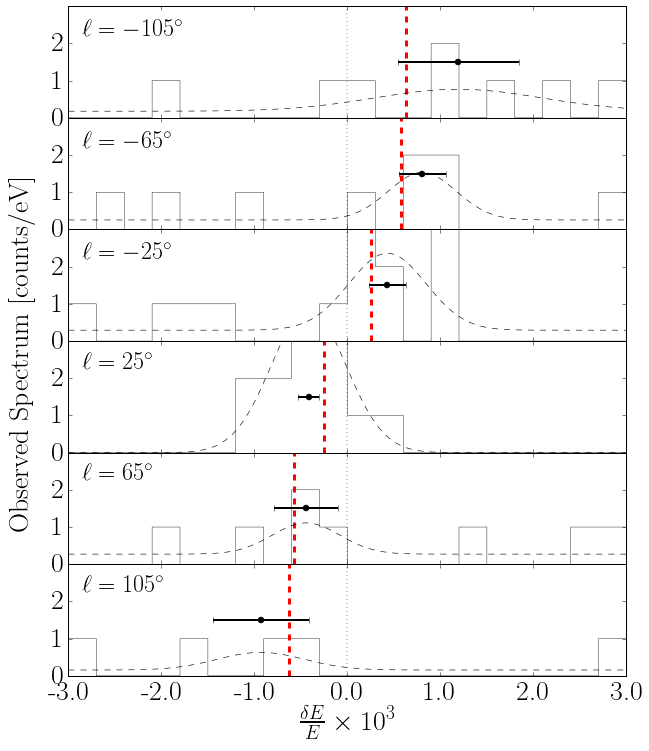
Our figure of merit for a detection of a Doppler-shifted line is the probability that the data exclude zero shifting. In other words, we consider the energy shift of the line centroid away from in units of , the uncertainty in the line energy.
Ref. [95] gives a prescription for obtaining the covariance matrix between the four fitted parameters, which we use to compute . This naturally incorporates the Poisson errors due to and , so that as expected. We obtain a global significance by summing the significances (the number of by which is excluded) for each pointing in quadrature.
IV Results
Our velocity spectroscopy analysis on N-body data reveals three main insights.


The first is that our analytic model matches the N-body calculation extremely well (). We summarize this result in Figure 4. Furthermore, the simple sinusoid model given by (corresponding to the limit in which the field of view radius goes to zero) also matches the analytic model for Micro-X to within a few percent over the entire range of (). This line-of-sight integral is thus a sufficient approximation to a large field of view instrument for the given exposure. Note that such small values are due to the large error bars from small . Since , these two models are only differentiable by observations times longer. This suggests that for further studies, this sinusoid model is more than sufficient and may be used to quickly explore the parameter space of haloes (e.g. with a Markov chain Monte Carlo) with minimal loss of precision.
The second main result is that combining the observed line energies from the six pointings modeled here ( with ) can exclude globally at . A constant line shift over various longitudes imply a detector artifact, and hence the significance of excluding a baryonic origin of the line is even higher. In synthetic observations as described in Section III.3, we find that 95% allow a detection of Doppler shifting. Repeating this experiment for a mission with 10x the exposure, we find that 95% of observations give a exclusion of . See Figure 5 for the full results of this test.
We also find that the effect of subhaloes on our observations are small, with only of pointings seeing over 10% of the flux contributed by a single subhalo (Figure 6). This supports intuition in that the perigee of subhaloes to the galactic center in our simulations is much larger than : Only 1% of subhaloes can be found within of the GC, so the smooth component of the main halo is expected to dominate the signal.
The pointings centered around exclude with the highest significance, at . This pointing optimizes between two competing effects. The first is the higher J-factor, hence higher photon flux, nearer the Galactic center, giving a smaller uncertainty in the energy of a line detected at small . The second is that the mean velocity along the line-of-sight relative to the dark matter increases with (up to ), shifting the observed line further from . We illustrate this effect using sky maps in Figure 7. Future observations should focus on these longitudes in order to achieve the best potential detection of this Doppler shift.
Finally, we find that halo triaxiality can bias the significance of a detection to the east or west of the Galactic center. When observing above the Galactic plane (in this work, ) any ellipticity of the Galactic halo on the sky can give a higher flux to one side of than the other. While the mean prediciton for the line centroid matches the analytic model for a spherical halo quite well, observing to one side of the GC allows one to exclude with higher significance due to better photon counting statistics. This is illustrated in Figure 8.


V Conclusions
Numerous times in the past, anomalous astrophysical signals have been interpreted as the signature of dark matter. So far, none of these extraordinary claims survived the scrutiny of extraordinary evidence. All of these false alarms raise an important question: can we design a new test to confirm the dark matter origin of an anomalous astrophysical signal?
For the case of a photon line, the answer is yes. Ref. [1] showed that telescopes with (0.1%) energy resolution can utilize the Doppler effect of a sharp signal arising from dark matter annihilation and decay to perform a particle physics model-independent test: dark matter velocity spectroscopy.
We look into the issue in this work using synthetic observations generated from a suite of N-body simulations [35]. An N-body simulation takes into account many complex processes which occur during galaxy formation, and these effects are not completely captured in an analytical description. It is essential to check the validity of any new signature with numerical simulations. We find that the phenomenon of dark matter velocity spectroscopy is robust while considering various dark matter only simulations of the Milky Way. Previous work had applied the technique to a narrow field of view instrument like Hitomi, whereas in this work we concentrate on a wide field of view instrument like Micro-X. We take the 3.5 keV line as our test case. We show that if Micro-X confirms the presence of the 3.5 keV line in our Galaxy, then it can also use dark matter velocity spectroscopy to confirm or refute the dark matter origin of the line.
For a Micro-X like instrument, the simple sinusoidal model for the Doppler shifting signature is sufficient (see Fig. 4). This agreement arises due to the small number of photon counts. We find that Micro-X (total exposure for all pointings) can reliably confirm the Doppler shifting effect on a sterile neutrino decay line at or better (see Figs. 5 and 7). The best design for such an observation consists of pointings centered around Galactic longitude and latitude , as this gives the optimal balance between the magnitude of the Doppler shift and the signal to noise ratio.
Typical sterile neutrino dark matter production mechanisms predict a large cutoff in the mass function, 108 M⊙. Thus, subhalos contribute little to the flux spectrum, and has no appreciable effect to velocity spectroscopy for sterile neutrino dark matter (see Fig. 6). Dark matter halos are predicted to be triaxial. We find that triaxiality has a large effect on velocity spectroscopy: the Doppler shift becomes asymmetric, and it results in a decrease of the signal significance (see Fig. 8).
Since we look at regions away from the Galactic Center, the signal rate is not maximum at these places. The observation strategy for any search should first focus on searching for a line at regions with higher signal to noise. The technique of dark matter velocity spectroscopy should be then applied at this specific line energy to confirm or refute the dark matter interpretation of this photon line.
We are optimistic about future experiments. While Micro-X is a good model for a first observation of dark matter velocity spectroscopy in the Milky Way, future high energy resolution telescopes are sure to provide the modest increase in photon counts needed for a high-significance detection. Increasing the Micro-X exposure by a factor of 10 gives at least an detection of the Doppler effect on photons arising from sterile neutrino decay.
The theoretical and observational concepts laid out in this work are general. Any sharp photon feature arising from dark matter annihilation or decay [96, 97] will get Doppler shifted in the above mentioned way. In addition to other indirect searches of dark matter (see for e.g., [98, 99, 100, 101, 102, 103, 104]), we expect that this new technique will be adopted widely. We encourage theorists, experimentalists and observers to optimize their tools to take advantage of this new and exciting smoking gun in motion signature of dark matter.
Acknowledgments
The authors thank John F. Beacom, Eric Charles, Joseph Conlon, Chris Davis, Matt Kistler, Dmytro Iakubovskyi, Mark Lovell, and Greg Madejski for helpful discussions. We especially thank Yao-Yuan Mao for help with the simulations. D.P. is thankful for support from the Stanford Fletcher Jones Foundation Fellowship. R.L. is supported by DOE Contract DE-AC02-76SF00515 in SLAC.
References
- [1] E. G. Speckhard, K. C. Y. Ng, J. F. Beacom, and R. Laha, Physical Review Letters 116, 031301 (2016), arXiv:1507.04744 .
- [2] G. Jungman, M. Kamionkowski, and K. Griest, Phys. Rept. 267, 195 (1996), arXiv:hep-ph/9506380 [hep-ph] .
- [3] G. Bertone, D. Hooper, and J. Silk, Phys. Rept. 405, 279 (2005), arXiv:hep-ph/0404175 [hep-ph] .
- [4] L. E. Strigari, Phys. Rept. 531, 1 (2013), arXiv:1211.7090 [astro-ph.CO] .
- [5] G. Bertone and D. Hooper, Submitted to: Rev. Mod. Phys. (2016), arXiv:1605.04909 [astro-ph.CO] .
- [6] M. Klasen, M. Pohl, and G. Sigl, Prog. Part. Nucl. Phys. 85, 1 (2015), arXiv:1507.03800 [hep-ph] .
- [7] J. M. Gaskins, (2016), arXiv:1604.00014 [astro-ph.HE] .
- [8] D. Elsaesser and K. Mannheim, Phys. Rev. Lett. 94, 171302 (2005), arXiv:astro-ph/0405235 [astro-ph] .
- [9] M. Loewenstein and A. Kusenko, Astrophys. J. 714, 652 (2010), arXiv:0912.0552 [astro-ph.HE] .
- [10] D. A. Prokhorov and J. Silk, Astrophys. J. 725, L131 (2010), arXiv:1001.0215 [astro-ph.HE] .
- [11] C. Weniger, JCAP 1208, 007 (2012), arXiv:1204.2797 [hep-ph] .
- [12] W.-C. Huang, A. Urbano, and W. Xue, (2013), arXiv:1307.6862 [hep-ph] .
- [13] C. Gordon and O. Macias, Phys. Rev. D88, 083521 (2013), [Erratum: Phys. Rev.D89,no.4,049901(2014)], arXiv:1306.5725 [astro-ph.HE] .
- [14] T. Daylan, D. P. Finkbeiner, D. Hooper, T. Linden, S. K. N. Portillo, N. L. Rodd, and T. R. Slatyer, Phys. Dark Univ. 12, 1 (2016), arXiv:1402.6703 [astro-ph.HE] .
- [15] K. N. Abazajian, N. Canac, S. Horiuchi, M. Kaplinghat, and A. Kwa, JCAP 1507, 013 (2015), arXiv:1410.6168 [astro-ph.HE] .
- [16] S. K. Lee, M. Lisanti, B. R. Safdi, T. R. Slatyer, and W. Xue, Phys. Rev. Lett. 116, 051103 (2016), arXiv:1506.05124 [astro-ph.HE] .
- [17] R. Bartels, S. Krishnamurthy, and C. Weniger, Phys. Rev. Lett. 116, 051102 (2016), arXiv:1506.05104 [astro-ph.HE] .
- [18] E. Bulbul, M. Markevitch, A. Foster, R. K. Smith, M. Loewenstein, and S. W. Randall, Astrophys. J. 789, 13 (2014a), arXiv:1402.2301 [astro-ph.CO] .
- [19] A. Boyarsky, O. Ruchayskiy, D. Iakubovskyi, and J. Franse, Phys. Rev. Lett. 113, 251301 (2014a), arXiv:1402.4119 [astro-ph.CO] .
- [20] O. Urban, N. Werner, S. W. Allen, A. Simionescu, J. S. Kaastra, and L. E. Strigari, Mon. Not. Roy. Astron. Soc. 451, 2447 (2015), arXiv:1411.0050 [astro-ph.CO] .
- [21] M. Ackermann et al. (Fermi-LAT), Phys. Rev. D88, 082002 (2013), arXiv:1305.5597 [astro-ph.HE] .
- [22] R. M. O’Leary, M. D. Kistler, M. Kerr, and J. Dexter, (2015), arXiv:1504.02477 [astro-ph.HE] .
- [23] M. Ackermann et al. (Fermi-LAT), Phys. Rev. D91, 122002 (2015), arXiv:1506.00013 [astro-ph.HE] .
- [24] T. D. Brandt and B. Kocsis, Astrophys. J. 812, 15 (2015), arXiv:1507.05616 [astro-ph.HE] .
- [25] R. M. O’Leary, M. D. Kistler, M. Kerr, and J. Dexter, (2016), arXiv:1601.05797 [astro-ph.HE] .
- [26] L. Gu, J. Kaastra, A. J. J. Raassen, P. D. Mullen, R. S. Cumbee, D. Lyons, and P. C. Stancil, Astron. Astrophys. 584, L11 (2015), arXiv:1511.06557 [astro-ph.HE] .
- [27] K. J. H. Phillips, B. Sylwester, and J. Sylwester, Astrophys. J. 809, 50 (2015).
- [28] C. Shah, S. Dobrodey, S. Bernitt, R. Steinbrugge, J. R. C. Lopez-Urrutia, L. Gu, and J. Kaastra, (2016), arXiv:1608.04751 [astro-ph.HE] .
- [29] B. Bozek, M. Boylan-Kolchin, S. Horiuchi, S. Garrison-Kimmel, K. Abazajian, and J. S. Bullock, Mon. Not. Roy. Astron. Soc. 459, 1489 (2016), arXiv:1512.04544 [astro-ph.CO] .
- [30] S. Horiuchi, B. Bozek, K. N. Abazajian, M. Boylan-Kolchin, J. S. Bullock, S. Garrison-Kimmel, and J. Onorbe, Mon. Not. Roy. Astron. Soc. 456, 4346 (2016), arXiv:1512.04548 [astro-ph.CO] .
- [31] T. Takahashi, K. Mitsuda, R. Kelley, F. Aharonian, H. Akamatsu, F. Akimoto, S. Allen, N. Anabuki, L. Angelini, K. Arnaud, and et al., in Space Telescopes and Instrumentation 2014: Ultraviolet to Gamma Ray, Proceedings of the SPIE Astronomical Instrumentation “Space Telescopes and Instrumentation 2014: Ultraviolet to Gamma Ray (2014).
- [32] D. McCammon et al., Astrophys. J. 576, 188 (2002), arXiv:astro-ph/0205012 [astro-ph] .
- [33] A. Boyarsky, J. W. den Herder, A. Neronov, and O. Ruchayskiy, Astropart. Phys. 28, 303 (2007), arXiv:astro-ph/0612219 [astro-ph] .
- [34] E. Figueroa-Feliciano et al. (XQC), Astrophys. J. 814, 82 (2015), arXiv:1506.05519 [astro-ph.CO] .
- [35] Y.-Y. Mao, M. Williamson, and R. H. Wechsler, Astrophys. J. 810, 21 (2015), arXiv:1503.02637 .
- [36] S. Riemer-Sorensen, Astron. Astrophys. 590, A71 (2016), arXiv:1405.7943 [astro-ph.CO] .
- [37] T. E. Jeltema and S. Profumo, Mon. Not. Roy. Astron. Soc. 450, 2143 (2015), arXiv:1408.1699 [astro-ph.HE] .
- [38] A. Boyarsky, J. Franse, D. Iakubovskyi, and O. Ruchayskiy, Phys. Rev. Lett. 115, 161301 (2015), arXiv:1408.2503 [astro-ph.CO] .
- [39] D. Malyshev, A. Neronov, and D. Eckert, Phys. Rev. D90, 103506 (2014), arXiv:1408.3531 [astro-ph.HE] .
- [40] P. D. Alvarez, J. P. Conlon, F. V. Day, M. C. D. Marsh, and M. Rummel, JCAP 1504, 013 (2015), arXiv:1410.1867 [hep-ph] .
- [41] M. E. Anderson, E. Churazov, and J. N. Bregman, Mon. Not. Roy. Astron. Soc. 452, 3905 (2015), arXiv:1408.4115 [astro-ph.HE] .
- [42] A. Boyarsky, J. Franse, D. Iakubovskyi, and O. Ruchayskiy, (2014b), arXiv:1408.4388 [astro-ph.CO] .
- [43] E. Bulbul, M. Markevitch, A. R. Foster, R. K. Smith, M. Loewenstein, and S. W. Randall, (2014b), arXiv:1409.4143 [astro-ph.HE] .
- [44] J. P. Conlon and A. J. Powell, JCAP 1501, 019 (2015), arXiv:1406.5518 [hep-ph] .
- [45] D. Iakubovskyi, (2014), arXiv:1410.2852 [astro-ph.HE] .
- [46] E. Carlson, T. Jeltema, and S. Profumo, JCAP 1502, 009 (2015), arXiv:1411.1758 [astro-ph.HE] .
- [47] T. Jeltema and S. Profumo, (2014), arXiv:1411.1759 [astro-ph.HE] .
- [48] T. Tamura, R. Iizuka, Y. Maeda, K. Mitsuda, and N. Y. Yamasaki, Publ. Astron. Soc. Jap. 67, 23 (2015), arXiv:1412.1869 [astro-ph.HE] .
- [49] D. Iakubovskyi, E. Bulbul, A. R. Foster, D. Savchenko, and V. Sadova, (2015), arXiv:1508.05186 [astro-ph.HE] .
- [50] N. Sekiya, N. Y. Yamasaki, and K. Mitsuda, Publ. Astron. Soc. Jap. (2015), 10.1093/pasj/psv081, arXiv:1504.02826 [astro-ph.HE] .
- [51] D. Iakubovskyi, Mon. Not. Roy. Astron. Soc. 453, 4097 (2015a), arXiv:1507.02857 [astro-ph.HE] .
- [52] S. Riemer-Sorensen et al., Astrophys. J. 810, 48 (2015), arXiv:1507.01378 [astro-ph.CO] .
- [53] D. Iakubovskyi, (2015b), arXiv:1510.00358 [astro-ph.HE] .
- [54] T. E. Jeltema and S. Profumo, Mon. Not. Roy. Astron. Soc. 458, 3592 (2016), arXiv:1512.01239 [astro-ph.HE] .
- [55] O. Ruchayskiy, A. Boyarsky, D. Iakubovskyi, E. Bulbul, D. Eckert, J. Franse, D. Malyshev, M. Markevitch, and A. Neronov, Mon. Not. Roy. Astron. Soc. 460, 1390 (2016), arXiv:1512.07217 [astro-ph.HE] .
- [56] E. Bulbul, M. Markevitch, A. Foster, E. Miller, M. Bautz, M. Loewenstein, S. W. Randall, and R. K. Smith, (2016), arXiv:1605.02034 [astro-ph.HE] .
- [57] F. A. Aharonian et al. (Hitomi), (2016), arXiv:1607.07420 [astro-ph.HE] .
- [58] F. Hofmann, J. S. Sanders, K. Nandra, N. Clerc, and M. Gaspari, Astron. Astrophys. 592, A112 (2016), arXiv:1606.04091 [astro-ph.CO] .
- [59] C. A. Arguelles, V. Brdar, and J. Kopp, (2016), arXiv:1605.00654 [hep-ph] .
- [60] J. P. Conlon, F. Day, N. Jennings, S. Krippendorf, and M. Rummel, (2016), arXiv:1608.01684 [astro-ph.HE] .
- [61] A. Neronov, D. Malyshev, and D. Eckert, (2016), arXiv:1607.07328 [astro-ph.HE] .
- [62] K. Perez, K. C. Y. Ng, J. F. Beacom, C. Hersh, S. Horiuchi, and R. Krivonos, (2016), arXiv:1609.00667 [astro-ph.HE] .
- [63] A. Gewering-Peine, D. Horns, and J. H. M. M. Schmitt, (2016), arXiv:1611.01733 [astro-ph.HE] .
- [64] T. M. Dame, D. Hartmann, and P. Thaddeus, Astrophys. J. 547, 792 (2001), arXiv:astro-ph/0009217 [astro-ph] .
- [65] R. Diehl et al., Nature 439, 45 (2006), arXiv:astro-ph/0601015 [astro-ph] .
- [66] P. M. W. Kalberla and L. Dedes, Astron. Astrophys. 487, 951 (2008), arXiv:0804.4831 [astro-ph] .
- [67] K. Kretschmer, R. Diehl, M. Krause, A. Burkert, K. Fierlinger, O. Gerhard, J. Greiner, and W. Wang, Astron. Astrophys. 559, A99 (2013), arXiv:1309.4980 [astro-ph.HE] .
- [68] M. S. Turner, Phys. Rev. D34, 1921 (1986).
- [69] D. Attie et al., Astronomy and Astrophysics 411, L71 (2003), arXiv:astro-ph/0308504 .
- [70] T. Takahashi et al., Proceedings, Space Telescopes and Instrumentation 2012: Ultraviolet to Gamma Ray: Amsterdam, Netherlands, July 1-6, 2012, Proc. SPIE Int. Soc. Opt. Eng. 8443, 84431Z (2012), arXiv:1210.4378 [astro-ph.IM] .
- [71] D. Barret et al., (2016), 10.1117/12.2232432, arXiv:1608.08105 [astro-ph.IM] .
- [72] Z. Wang and M. Xu, Proceedings of 16th International Conference on Calorimetry in High Energy Physics (CALOR 2014): Giessen, Germany, April 6-11, 2014, J. Phys. Conf. Ser. 587, 012027 (2015).
- [73] X. Huang et al., Astropart. Phys. 78, 35 (2016), arXiv:1509.02672 [astro-ph.HE] .
- [74] F. S. Ling, E. Nezri, E. Athanassoula, and R. Teyssier, JCAP 1002, 012 (2010), arXiv:0909.2028 [astro-ph.GA] .
- [75] M. Kuhlen, A. Pillepich, J. Guedes, and P. Madau, Astrophys. J. 784, 161 (2014), arXiv:1308.1703 [astro-ph.GA] .
- [76] I. Butsky, A. V. Maccio, A. A. Dutton, L. Wang, G. S. Stinson, C. Penzo, X. Kang, B. W. Keller, and J. Wadsley, (2015), arXiv:1503.04814 [astro-ph.GA] .
- [77] N. Bozorgnia, F. Calore, M. Schaller, M. Lovell, G. Bertone, C. S. Frenk, R. A. Crain, J. F. Navarro, J. Schaye, and T. Theuns, JCAP 1605, 024 (2016), arXiv:1601.04707 [astro-ph.CO] .
- [78] J. D. Sloane, M. R. Buckley, A. M. Brooks, and F. Governato, (2016), arXiv:1601.05402 [astro-ph.GA] .
- [79] C. Kelso, C. Savage, M. Valluri, K. Freese, G. S. Stinson, and J. Bailin, (2016), arXiv:1601.04725 [astro-ph.GA] .
- [80] V. Springel, M.N.R.A.S. 364, 1105 (2005), arXiv:astro-ph/0505010 .
- [81] X.-D. Shi and G. M. Fuller, Phys. Rev. Lett. 82, 2832 (1999), arXiv:astro-ph/9810076 [astro-ph] .
- [82] T. Venumadhav, F.-Y. Cyr-Racine, K. N. Abazajian, and C. M. Hirata, Phys. Rev. D 94, 043515 (2016), arXiv:1507.06655 .
- [83] M. R. Lovell, G. Bertone, A. Boyarsky, A. Jenkins, and O. Ruchayskiy, Mon. Not. Roy. Astron. Soc. 451, 1573 (2015), arXiv:1411.0311 [astro-ph.CO] .
- [84] A. Merle and A. Schneider, Phys. Lett. B749, 283 (2015), arXiv:1409.6311 [hep-ph] .
- [85] J. Arvo, “Fast random rotation matrices,” (1992).
- [86] V. P. Debattista, B. Moore, T. R. Quinn, S. Kazantzidis, R. Maas, L. Mayer, J. Read, and J. Stadel, Astrophys. J. 681, 1076 (2008), arXiv:0707.0737 [astro-ph] .
- [87] S. E. Bryan, S. T. Kay, A. R. Duffy, J. Schaye, C. D. Vecchia, and C. M. Booth, Mon. Not. Roy. Astron. Soc. 429, 3316 (2013), arXiv:1207.4555 [astro-ph.CO] .
- [88] N. Bernal, J. E. Forero-Romero, R. Garani, and S. Palomares-Ruiz, JCAP 1409, 004 (2014), arXiv:1405.6240 [astro-ph.CO] .
- [89] N. Bernal, L. Necib, and T. R. Slatyer, (2016), arXiv:1606.00433 [astro-ph.CO] .
- [90] Y.-Y. Mao, L. E. Strigari, R. H. Wechsler, H.-Y. Wu, and O. Hahn, Astrophys. J. 764, 35 (2013), arXiv:1210.2721 [astro-ph.CO] .
- [91] S. G. Crowder et al., Astrophys. J. 758, 143 (2012), arXiv:1209.1657 [astro-ph.HE] .
- [92] M. Ajello et al., Astrophys. J. 689, 666 (2008), arXiv:0808.3377 [astro-ph] .
- [93] A. Moretti, C. Pagani, G. Cusumano, S. Campana, M. Perri, A. Abbey, M. Ajello, A. P. Beardmore, D. Burrows, G. Chincarini, O. Godet, C. Guidorzi, J. E. Hill, J. Kennea, J. Nousek, J. P. Osborne, and G. Tagliaferri, Astronomy and Astrophysics 493, 501 (2009).
- [94] H. Tomida, D. Uchida, H. Tsunemi, R. Imatani, M. Kimura, S. Nakahira, T. Hanayama, and K. Yoshidome, (2016), 10.1093/pasj/psw006, arXiv:1602.01229 [astro-ph.HE] .
- [95] R. Barlow, Nuclear Instruments and Methods in Physics Research Section A: Accelerators, Spectrometers, Detectors and Associated Equipment 297, 496 (1990).
- [96] K. K. Boddy and J. Kumar, Phys. Rev. D92, 023533 (2015), arXiv:1504.04024 [astro-ph.CO] .
- [97] A. Ibarra, H. M. Lee, S. Lopez Gehler, W.-I. Park, and M. Pato, JCAP 1305, 016 (2013), [Erratum: JCAP1603,no.03,E01(2016)], arXiv:1303.6632 [hep-ph] .
- [98] H. Yuksel and M. D. Kistler, Phys. Rev. D78, 023502 (2008), arXiv:0711.2906 [astro-ph] .
- [99] B. Dasgupta and R. Laha, Phys. Rev. D86, 093001 (2012), arXiv:1206.1322 [hep-ph] .
- [100] R. Laha, K. C. Y. Ng, B. Dasgupta, and S. Horiuchi, Phys. Rev. D87, 043516 (2013), arXiv:1208.5488 [astro-ph.CO] .
- [101] K. C. Y. Ng, R. Laha, S. Campbell, S. Horiuchi, B. Dasgupta, K. Murase, and J. F. Beacom, Phys. Rev. D89, 083001 (2014), arXiv:1310.1915 [astro-ph.CO] .
- [102] K. Murase, R. Laha, S. Ando, and M. Ahlers, Phys. Rev. Lett. 115, 071301 (2015), arXiv:1503.04663 [hep-ph] .
- [103] K. C. Y. Ng, S. Horiuchi, J. M. Gaskins, M. Smith, and R. Preece, Phys. Rev. D92, 043503 (2015), arXiv:1504.04027 [astro-ph.CO] .
- [104] D. Chowdhury, A. M. Iyer, and R. Laha, (2016), arXiv:1601.06140 [hep-ph] .