1Introduction

Toward a Holographic Theory for General Spacetimes

Yasunori Nomura^a,b, Nico Salzetta^a,b, Fabio Sanches^a,b, and Sean J. Weinberg^c

^a Berkeley Center for Theoretical Physics, Department of Physics,
University of California, Berkeley, CA 94720, USA

^b Theoretical Physics Group, Lawrence Berkeley National Laboratory, CA 94720, USA

^c Department of Physics, University of California, Santa Barbara, CA 93106, USA

We study a holographic theory of general spacetimes that does not rely on the existence of asymptotic regions. This theory is to be formulated in a holographic space. When a semiclassical description is applicable, the holographic space is assumed to be a holographic screen: a codimension-1 surface that is capable of encoding states of the gravitational spacetime. Our analysis is guided by conjectured relationships between gravitational spacetime and quantum entanglement in the holographic description. To understand basic features of this picture, we catalog predictions for the holographic entanglement structure of cosmological spacetimes. We find that qualitative features of holographic entanglement entropies for such spacetimes differ from those in AdS/CFT but that the former reduce to the latter in the appropriate limit. The Hilbert space of the theory is analyzed, and two plausible structures are found: a direct sum and “spacetime equals entanglement” structure. The former preserves a naive relationship between linear operators and observable quantities, while the latter respects a more direct connection between holographic entanglement and spacetime. We also discuss the issue of selecting a state in quantum gravity, in particular how the state of the multiverse may be selected in the landscape.

1 Introduction

As with any other classical object, spacetime is expected to consist of a large number of quantum degrees of freedom. The first explicit hint of this came from the discovery that empty spacetime can carry entropy [1, 2, 3, 4, 5, 6]. What theory describes these degrees of freedom as well as the excitations on them, i.e. matter?

Part of the difficulty in finding such a theory is the large redundancies present in the description of gravitational spacetime. The holographic principle [7, 8, 9] suggests that the natural space in which the microscopic degrees of freedom for spacetime (and matter) live is a non-dynamical spacetime whose dimension is one less than that in the original description (as demonstrated in the special case of the AdS/CFT correspondence [10]). This represents a huge redundancy in the original gravitational description beyond that associated with general coordinate transformations. For general spacetimes, causality plays a central role in fixing this redundancy [11, 12]. A similar idea also plays an important role in addressing problems in the semiclassical descriptions of black holes [13] and cosmology [14, 15].

In this paper, we explore a holographic theory for general spacetimes. We follow a “bottom-up” approach given the lack of a useful description in known frameworks, such as AdS/CFT and string theory in asymptotically Minkowski space. We assume that our holographic theory is formulated on a holographic screen [16], a codimension-1 surface on which the information about the original spacetime can be encoded. This construction can be extended beyond the semiclassical regime by considering all possible states on all possible slices—called leaves—of holographic screens [14, 17], where the nonuniqueness of erecting a holographic screen is interpreted as the freedom in fixing the redundancy associated with holography. The resulting picture is consistent with the recently discovered area theorem applicable to the holographic screens [18, 19, 20].

To study the structure of the theory, we use conjectured relationships between spacetime in the gravitational description and quantum entanglement in the holographic theory. Recently, it has become increasingly clear that quantum entanglement among holographic degrees of freedom plays an important role in the emergence of classical spacetime [21, 22, 23, 24, 25, 26, 27, 28, 29, 30, 31, 32]. In particular, Ref. [28] showed that the areas of the extremal surfaces anchored to the boundaries of regions on a leaf of a holographic screen satisfy relations obeyed by entanglement entropies, so that they can indeed be identified as the entanglement entropies associated with the corresponding regions in the holographic space. We analyze properties of these surfaces and discuss their implications for a holographic theory of general spacetimes.

We lay down our general framework in Section 2. We then study the behavior of extremal surfaces in cosmological Friedmann-Robertson-Walker (FRW) spacetimes in Section 3. Here we focus on initially expanding flat and open universes, in which the area of the leaves monotonically increases. We first consider universes dominated by a single component in the Friedmann equation, and we identify how screen entanglement entropies—the entanglement entropies among the degrees of freedom in the holographic space—encode information about the spacetimes. We discuss next how the screen entanglement entropies behave in a transition period in which the dominant component of the universe changes. We find an interesting theorem when the holographic screen is spacelike: the change of a screen entanglement entropy is always monotonic. The proof of this theorem is given in Appendix A. If the holographic screen is timelike, no such theorem holds.

In Section 4, we study the structure of the holographic theory for general spacetimes, building on the results obtained earlier. In particular, we discuss how the holographic entanglement entropies for general spacetimes differ from those in AdS/CFT and how, nevertheless, the former reduce to the latter in an appropriate limit. We emphasize that the holographic entanglement entropies for cosmological spacetimes obey a volume law, rather than an area law, implying that the relevant holographic states are not ground states of local field theories. This is the case despite the fact that the dynamics of the holographic theory respects some sense of locality, indicated by the fact that the area of a leaf increases in a local manner on a holographic screen.

The Hilbert space of the theory is analyzed in Section 4.2 under two assumptions:

(i)

The holographic theory has (effectively) a qubit degree of freedom per each volume of $4\ln 2$ in Planck units. These degrees of freedom appear local at lengthscales larger than a microscopic cutoff $l_{\rm c}$ .
(ii)

If a holographic state represents a semiclassical spacetime, the area of an extremal surface anchored to the boundary of a region $\Gamma$ on a leaf $\sigma$ and contained in the causal region associated with $\sigma$ represents the entanglement entropy of $\Gamma$ in the holographic theory.

We find that these two assumptions strongly constrain the structure of the Hilbert space, although they do not determine it uniquely. There are essentially two possibilities:

Direct sum structure — Holographic states representing different semiclassical spacetimes ${\cal M}$ live in different Hilbert spaces ${\cal H}_{\cal M}$ even if these spacetimes have the same boundary space (or leaf) $B$

${\cal H}_{B}=\bigoplus_{\cal M}{\cal H}_{\cal M}.$ (1)

In each Hilbert space ${\cal H}_{\cal M}$ , the states representing the semiclassical spacetime comprise only a tiny subset of all the states—the vast majority of the states in ${\cal H}_{\cal M}$ do not allow for a semiclassical interpretation, which we call “firewall” states borrowing the terminology in Refs. [33, 34, 35]. In fact, the states allowing for a semiclassical spacetime interpretation do not even form a vector space—their superposition may lead to a firewall state if it involves a large number of terms, of order a positive power of ${\rm dim}\,{\cal H}_{\cal M}$ . This is because a superposition involving such a large number of terms significantly alters the entanglement entropy structure, so under assumption (ii) above we cannot interpret the resulting state as a semiclassical state representing ${\cal M}$ . In this picture, small excitations over spacetime ${\cal M}$ can be represented by standard linear operators acting on the (suitably extended) Hilbert space ${\cal H}_{\cal M}$ , which can be trivially promoted to linear operators in ${\cal H}_{B}$ .

Spacetime equals entanglement — Holographic states that represent different semiclassical spacetimes but have same boundary space $B$ are all elements of a single Hilbert space ${\cal H}_{B}$ . And yet, the number of independent microstates representing each of these spacetimes, ${\cal M},{\cal M}^{\prime},{\cal M}^{\prime\prime},\cdots$ , is the dimension of ${\cal H}_{B}$ :

|\Psi^{\cal M}_{i}\rangle,\,\,|\Psi^{{\cal M}^{\prime}}_{i^{\prime}}\rangle,\,\,|\Psi^{{\cal M}^{\prime\prime}}_{i^{\prime\prime}}\rangle,\,\,\cdots\,\in\,{\cal H}_{B};\qquad i,i^{\prime},i^{\prime\prime},\cdots=1,\cdots,{\rm dim}\,{\cal H}_{B},

(2)

which implies that the microstates representing different spacetimes are not independent. This picture arises if we require the converse of assumption (ii) and is called “spacetime equals entanglement” [31]: if a holographic state has the form of entanglement entropies corresponding to a certain spacetime, then the state indeed represents that spacetime. The structure of Eq. (2) is then obtained because arbitrary unitary transformations acting in each cutoff size cell in $B$ do not change the entanglement entropies, implying that the number of microstates for any geometry is ${\rm dim}\,{\cal H}_{B}$ (so they span a basis of ${\cal H}_{B}$ ). Despite the intricate structure of the states, this picture admits the standard many worlds interpretation for classical spacetimes, as shown in Ref. [31]. Small excitations over spacetime are represented by non-linear/state-dependent operators, along the lines of Ref. [36] (see also [37, 38, 39]), since a superposition of background spacetimes may lead to another spacetime, so that operators representing excitations must know the entire quantum state they act on.

We note that a dichotomy similar to the one described above was discussed earlier in Ref. [36], but the interpretation and the context in which it appears here are distinct. First, the state-dependence of the operators representing excitations in the second scenario (as well as that of the time evolution operator) becomes relevant when the boundary space is involved in the dynamics as in the case of cosmological spacetimes. Hence, this particular state-dependence need not persist in the AdS/CFT limit. This does not imply anything about the description of the interior a black hole in the CFT. It is possible that the CFT does not provide a semiclassical description of the black hole interior, i.e. it gives only a distant description. Alternatively, there may be a way of obtaining a state-dependent semiclassical description of the black hole interior within a CFT, as envisioned in Ref. [36]. We are agnostic about this issue.

Second, Ref. [36] describes the dichotomy as state-dependence vs. firewalls. Our picture, on the other hand, does not have a relation with firewalls because the following two statements apply to both the direct sum and spacetime equals entanglement pictures:

•

Most of the states in the Hilbert space, e.g. in the Haar measure, are firewalls in the sense that they do not represent smooth semiclassical spacetimes, which require special entanglement structures among the holographic degrees of freedom.
•

The fact that most of the states are firewalls does not mean that these states are realized as a result of standard time evolution, in which the volume of the boundary space increases in time. In fact, the direct sum picture even has a built-in mechanism of eliminating firewalls through time evolution, as we will see in Section 4.5.¹¹ 1 This is natural because any dynamics leading to classicalization selects only a very special set of states as the result of time evolution: states interpreted as a superposition of a small number of classical worlds, where small means a number (exponentially) smaller than the dimension of the full microscopic Hilbert space.

Rather, the real tension is between the linearity/state-independence of operators representing observables (including the time evolution operator) and the spacetime equals entanglement hypothesis, i.e. the hypothesis that if a holographic state has entanglement entropies corresponding to a semiclassical spacetime, then the state indeed represents that spacetime. If we insist on the linearity of observables, we are forced to take the direct sum picture; if we adopt the spacetime equals entanglement hypothesis, then we must give up linearity.

Our analysis in Section 4 also includes the following. In Section 4.3, we discuss bulk reconstruction from a holographic state, which suggests that the framework provides a distant description for a dynamical black hole. In Section 4.4, we consider how the theory encodes information about spacetime outside the causal region of a leaf, which is needed for autonomous time evolution. Our analysis suggests a strengthened covariant entropy bound: the entropy on the union of two light sheets (future-directed ingoing and past-directed outgoing) of a leaf is bounded by the area of the leaf divided by $4$ . This bound is stronger than the original bound in Ref. [12], which says that the entropy on each of the two light sheets is bounded by the area divided by $4$ . In Section 4.5, we analyze properties of time evolution, in particular a built-in mechanics of eliminating firewalls in the direct sum picture and the required non-linearity of the time evolution operator in the spacetime equals entanglement picture. In Sections 4.4 and 4.5, we discuss how our framework may reduce to AdS/CFT and string theory in an asymptotically Minkowski background in the appropriate limits. We argue that the dynamics of these theories (in which the boundaries are sent to infinity) describe that of the general holographic theory modded out by “vacuum degeneracies” relevant for the dynamics of the boundaries and the exteriors.

In Section 5, we devote our final discussion to the issue of selecting a state. In general, specifying a system requires selection conditions on a state in addition to determining the theory. To address this issue in quantum gravity, we need to study the problem of time [40, 41]. We discuss possible signals from a past singularity or past null infinity, closed universes and “fine-tuning” of states, and selection conditions for the string theory landscape [42, 43, 44, 45], especially the scenario called the “static quantum multiverse” [46]. While our discussion in this section is schematic, it allows us to develop intuition about how quantum gravity might work at the fundamental level when applied to the real world.

Throughout the paper, we adopt the Schrödinger picture of quantum mechanics and take the Planck length to be unity, $l_{\rm P}=1$ . When the semiclassical picture is applicable, we assume the null and causal energy conditions to be satisfied. These impose the conditions $\rho\geq-p$ and $|\rho|\geq|p|$ , respectively, on the energy density $\rho$ and pressure $p$ of an ideal fluid component. The equation of state parameter $w=p/\rho$ , therefore, takes a value in the range $|w|\leq 1$ .

2 Holography and Quantum Gravity

The holographic principle states that quantum mechanics of a system with gravity can be formulated as a non-gravitational theory in spacetime with dimension one less than that in the gravitational description. The covariant entropy bound, or Bousso bound, [12] suggests that this holographically reduced—or “boundary”—spacetime may be identified as a hypersurface in the original gravitational spacetime determined by a collection of light rays. Specifically, it implies that the entropy on a null hypersurface generated by a congruence of light rays terminating at a caustic or singularity is bounded by its largest cross sectional area ${\cal A}$ ; in particular, the entropy on each side of the largest cross sectional surface is bounded by ${\cal A}/4$ in Planck units.²² 2 We will conjecture a stronger bound in Section 4.4. It is therefore natural to consider that, for a fixed gravitational spacetime, the holographic theory lives on a hypersurface—called the holographic screen—on which null hypersurfaces foliating the spacetime have the largest cross sectional areas [16].

This procedure of erecting a holographic screen has a large ambiguity, presumably reflecting a large freedom in fixing the redundancy of the gravitational description associated with the holographic principle. A particularly useful choice advocated in Refs. [14, 17, 47] is to adopt an “observer centric reference frame.” Let the origin of the reference frame follow a timelike curve $p(\tau)$ which passes through a fixed spacetime point $p_{0}$ at $\tau=0$ , and consider the congruence of past-directed light rays emanating from $p_{0}$ .³³ 3 In Refs. [14, 17, 47], $p(\tau)$ was chosen to be a timelike geodesic with $\tau$ being the proper time measured at $p(\tau)$ . We suspect that this simplifies the time evolution operator in the holographic theory. The expansion of the light rays $\theta$ satisfies

\frac{\partial\theta}{\partial\lambda}+\frac{1}{2}\theta^{2}\leq 0,

(3)

where $\lambda$ is the affine parameter associated with the light rays. This implies that the light rays emitted from $p_{0}$ focus toward the past (starting from $\theta=+\infty$ at $\lambda=0_{+}$ ), and we may identify the apparent horizon, i.e. the codimension-2 surface with

\theta=0,

(4)

to be an equal-time hypersurface—called a leaf—of a holographic screen. Repeating the procedure for all $\tau$ , we obtain a specific holographic screen, with the leaves parameterized by $\tau$ , corresponding to foliating the spacetime region accessible to the observer at $p(\tau)$ ; see Fig. 1. Such a foliation is consonant with the complementarity hypothesis [13], which asserts that a complete description of a system is obtained by referring only to the spacetime region that can be accessed by a single observer.

Refer to caption — Figure 1: For a fixed semiclassical spacetime, the holographic screen is a hypersurface obtained as the collection of codimension-2 surfaces (labeled by $\tau$ ) on which the expansion of the light rays emanating from a timelike curve $p(\tau)$ vanishes, $\theta=0$ . This way of erecting the holographic screen automatically deals with the redundancy associated with complementarity. The ambiguity of choosing $p(\tau)$ reflects a large freedom in fixing the redundancy associated with holography.

With this construction, we can view a quantum state of the holographic theory as living on a leaf of the holographic screen obtained in the above observer centric manner. We can then consider the collection of all possible quantum states on all possible leaves, obtained by considering all timelike curves in all spacetimes. We take the view that a state of quantum gravity lives in the Hilbert space spanned by all of these states (together with other states that do not admit a full spacetime interpretation) [14, 17]. It is often convenient to consider a Hilbert space ${\cal H}_{B}$ spanned by the holographic states that live on the “same” boundary space $B$ .⁴⁴ 4 The exact way in which the boundary spaces are grouped into different $B$ ’s is unimportant. For example, one can regard the boundary spaces having the same area ${\cal A}$ within some precision $\delta{\cal A}$ to be in the same $B$ , or one can discriminate them further by their induced metrics. This ambiguity does not affect any of the results, unless one takes $\delta{\cal A}$ to be exponentially small in ${\cal A}$ or discriminates induced metrics with the accuracy of order the Planck length (which corresponds to resolving microstates of the spacetime). The relevant Hilbert space can then be written as

{\cal H}=\sum_{B}{\cal H}_{B},

(5)

where the sum of Hilbert spaces is defined by⁵⁵ 5 Unlike Ref. [17], here we do not assume specific relations between ${\cal H}_{B}$ ’s; for example, ${\cal H}_{B_{1}}$ and ${\cal H}_{B_{2}}$ for different boundary spaces $B_{1}$ and $B_{2}$ may not be orthogonal. Also, we have included in the sum over $B$ the cases in which $B$ is outside the semiclassical regime, i.e. the cases in which the holographic space does not correspond to a leaf of a holographic screen in a semiclassical regime. These issues will be discussed in Section 4.

{\cal H}_{1}+{\cal H}_{2}=\{v_{1}+v_{2}\,|\,v_{1}\in{\cal H}_{1},v_{2}\in{\cal H}_{2}\}.

(6)

This formulation is not restricted to descriptions based on fixed semiclassical spacetime backgrounds. For example, we may consider a state in which macroscopically different spacetimes are superposed; in particular, this picture describes the eternally inflating multiverse as a state in which macroscopically different universes are superposed [14, 46]. The space in Eq. (5) is called the covariant Hilbert space with observer centric gauge fixing.

Recently, Bousso and Engelhardt have identified two special classes of holographic screens [18, 19]: if a portion of a holographic screen is foliated by marginally anti-trapped (trapped) surfaces, then that portion is called a past (future) holographic screen. Specifically, denoting the two future-directed null vector fields orthogonal to a portion of a leaf by $k^{a}$ and $l^{a}$ , with $k^{a}$ being tangent to light rays emanating from $p(\tau)$ , the expansion of the null geodesic congruence generated by $l^{a}$ satisfies $\theta_{l}>0$ and $<0$ for past and future holographic screens, respectively. They proved, building on earlier works [48, 49, 50, 51], that the area of leaves ${\cal A}(\tau)$ monotonically increases (decreases) for a past (future) holographic screen:

\left\{\begin{array}[]{l}\theta_{k}=0\\ \theta_{l}\gtrless 0\end{array}\right.\quad\Leftrightarrow\qquad\frac{d}{d\tau}{\cal A}(\tau)\gtrless 0;

(7)

see Fig. 2.

In many regular circumstances, including expanding FRW universes, the holographic screen is a past holographic screen, so that the area of the leaves monotonically increases, $d{\cal A}(\tau)/d\tau>0$ . In this paper we mostly focus on this case, and we interpret the area theorem in terms of the second law of thermodynamics applied to the Hilbert space of Eq. (5). Moreover, in Ref. [20] it was proved that this area theorem holds locally on the holographic screen: the area of any fixed spatial portion of the holographic screen, determined by a vector field tangent to the holographic screen and normal to its leaves, increases monotonically in time. This implies that the dynamics of the holographic theory respects some notion of locality.

What is the structure of the holographic theory and how can we explore it? Recently, a conjecture has been made in Ref. [28] which relates geometries of general spacetimes in the gravitational description to the entanglement entropies of states in the holographic theory. This extends the analogous theorem/conjecture in the AdS/CFT context [21, 22, 23] to more general cases, allowing us to probe the holographic description of general spacetimes, including those that do not have an obvious spacetime boundary on which the holographic theory can live. In particular, Ref. [28] proved that for a given region $\Gamma$ of a leaf $\sigma$ , a codimension-2 extremal surface $E(\Gamma)$ anchored to the boundary $\partial\Gamma$ of $\Gamma$ is fully contained in the causal region $D_{\sigma}$ of $\sigma$ :

D_{\sigma}:\,\,\mbox{the domain of dependence of an interior achronal hypersurface whose only boundary is $\sigma$},

(8)

where the concept of the interior is defined so that a vector on $\sigma$ pointing toward the interior takes the form $c_{1}k^{a}-c_{2}l^{a}$ with $c_{1},c_{2}>0$ (see Fig. 2). This implies that the normalized area of the extremal surface $E(\Gamma)$

S(\Gamma)=\frac{1}{4}\lVert E(\Gamma)\rVert,

(9)

satisfies expected properties of entanglement entropy, such as strong subadditivity, so that it can be identified with the entanglement entropy of the region $\Gamma$ in the holographic theory. Here, $\lVert x\rVert$ represents the area of $x$ . If there are multiple extremal surfaces in $D_{\sigma}$ for a given $\Gamma$ , then we must take the one with the minimal area.

In the rest of the paper, we study the holographic theory of quantum gravity for general spacetimes, adopting the framework described in this section. We first analyze FRW spacetimes and then discuss lessons learned from that analysis later.

3 Holographic Description of FRW Universes

In this section, we study the putative holographic description of $(3+1)$ -dimensional FRW cosmological spacetimes:

ds^{2}=-dt^{2}+a^{2}(t)\left[\frac{dr^{2}}{1-\kappa r^{2}}+r^{2}(d\psi^{2}+\sin^{2}\!\psi\,d\phi^{2})\right],

(10)

where $a(t)$ is the scale factor, and $\kappa<0$ , $=0$ and $>0$ for open, flat and closed universes, respectively. The Friedmann equation is given by

\left(\frac{\dot{a}}{a}\right)^{2}+\frac{\kappa}{a^{2}}=\frac{8\pi}{3}\rho,

(11)

where the dot represents $t$ derivative. Here, we include the energy density from the cosmological constant as a component in $\rho$ having the equation of state parameter $w=-1$ .

As discussed in the previous section, we describe the system as viewed from a reference frame whose origin follows a timelike curve $p(\tau)$ , which we choose to be at $r=0$ . The holographic theory then lives on the holographic screen, an equal-time slice of which is an apparent horizon: a codimension-2 surface on which the expansion of the light rays emanating from $p(\tau)$ for a fixed $\tau$ vanishes. Under generic conditions, this horizon is always at a finite distance

r=\frac{1}{\sqrt{\dot{a}^{2}(t_{*})+\kappa}}\equiv r_{\rm AH}(t_{*})<\infty,

(12)

where $t_{*}$ is the FRW time on the horizon. Note that the symmetry of the setup makes the FRW time the same everywhere on the apparent horizon, and for an open universe, $\dot{a}(t_{*})>\sqrt{-\kappa}$ is satisfied for values of $\tau$ before $p(\tau)$ hits the big crunch. For flat and open universes, we find that this surface is always marginally anti-trapped, i.e. a leaf of a past holographic screen, as long as the universe is initially expanding. On the other hand, for a closed universe the surface can change from marginally anti-trapped to marginally trapped as $\tau$ increases, implying that the holographic screen may be a past holographic screen only until certain time $\tau$ . In this section, we focus our attention on initially expanding flat and open universes. Closed universes will be discussed in Section 5.

Below, we study entanglement entropies for subregions in the holographic theory—screen entanglement entropies—adopting the conjecture of Ref. [28]. Here we focus on studying the properties of these entropies, leaving their detailed interpretation for later. We first discuss “stationary” aspects of screen entanglement entropies, concentrating on states representing spacetime in which the expansion of the universe is dominated by a single component in the Friedmann equation. We study how screen entanglement entropies encode the information about the spacetime the state represents. We then analyze dynamics of screen entanglement entropies during a transition period in which the dominant component changes. Implications of these results in the broader context of the holographic description of quantum gravity will be discussed in the next section.

3.1 Holographic dictionary for FRW universes

Consider a Hilbert space ${\cal H}_{B}$ spanned by a set of quantum states living in the same codimension-2 boundary surface $B$ . As mentioned in footnote 4, the definition of the boundary surface being the same has an ambiguity. For our analysis of states representing FRW spacetimes, we take the boundary $B$ to be specified by its area ${\cal A}_{B}$ (within some precision $\delta{\cal A}_{B}$ that is not exponentially small in ${\cal A}_{B}$ ). In this subsection, we focus on a single Hilbert space ${\cal H}_{*}\in\{{\cal H}_{B}\}$ specified by a fixed (though arbitrary) boundary area ${\cal A}_{*}$ .

Consider FRW universes with $\kappa\leq 0$ having vacuum energy $\rho_{\Lambda}$ and filled with varying ideal fluid components.⁶⁶ 6 The $\rho_{\Lambda}$ here represents the energy density of a (local) minimum of the potential near which fields in the FRW universe in question take values. In fact, string theory suggests that there is no absolutely stable de Sitter vacuum in full quantum gravity; it must decay, at least, before the Poincaré recurrence time [43]. For every universe with

\rho_{\Lambda}<\frac{3}{2{\cal A}_{*}},

(13)

there is an FRW time $t_{*}$ at which the area of the leaf of the past holographic screen is ${\cal A}_{*}$ ; see Fig. 3.

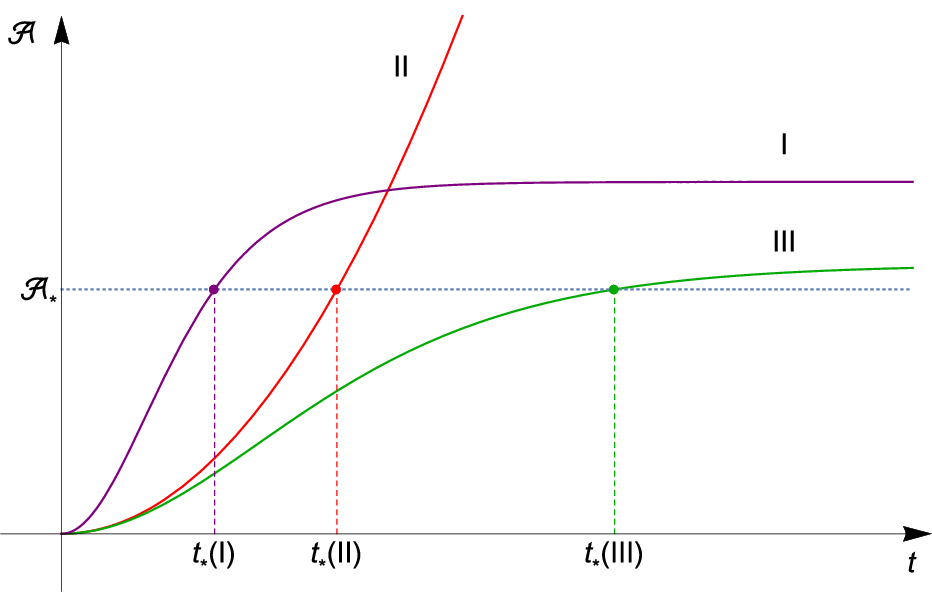
This is because the area of the leaf of the past holographic screen is monotonically increasing [18], and the final (asymptotic) value of the area is given by

{\cal A}_{\infty}=\left\{\begin{array}[]{ll}\frac{3}{2\rho_{\Lambda}},&\mbox{ for }\rho_{\Lambda}>0,\\ +\infty,&\mbox{ for }\rho_{\Lambda}\leq 0.\end{array}\right.

(14)

Any quantum state representing the system at any such moment is an element of ${\cal H}_{*}$ . A question is what features of the holographic state encode information about the universe it represents.

To study this problem, we perform the following analysis. First, given an FRW universe specified by the history of the energy density of the universe, $\rho(t)$ , we determine the FRW time $t_{*}$ at which the apparent horizon $\sigma_{*}$ , identified as a leaf of the past holographic screen, has the area ${\cal A}_{*}$ :

\left\{\begin{array}[]{l}\rho(t)\\ {\cal A}_{*}\end{array}\right.\rightarrow\,\,t_{*},

(15)

where we assume Eq. (13). We then consider a spherical cap region of the leaf $\sigma_{*}$ specified by an angle $\gamma$ ( $0\leq\gamma\leq\pi$ ):

L(\gamma):\ \,\,t=t_{*},\quad r=r_{\rm AH}(t_{*}),\quad 0\leq\psi\leq\gamma,

(16)

where $r_{\rm AH}(t_{*})$ is given by Eq. (12) (see Fig. 4), and determine the extremal surface $E(\gamma)$ which is codimension-2 in spacetime, anchored on the boundary of $L(\gamma)$ , and fully contained inside the causal region $D_{\sigma_{*}}$ associated with $\sigma_{*}$ .

According to Ref. [28], we interpret the quantity

S(\gamma)=\frac{1}{4}\lVert E(\gamma)\rVert,

(17)

to represent von Neumann entropy of the holographic state representing the region $L(\gamma)$ , obtained after tracing out the complementary region on $\sigma_{*}$ .

To determine the extremal surface $E(\gamma)$ , it is useful to introduce cylindrical coordinates

\xi=r\sin\psi,\qquad z=r\cos\psi.

(18)

We find that the isometry of the FRW metric, Eq. (10), allows us to move the boundary on which the extremal surface is anchored, $\partial L(\gamma)$ , on the $z=0$ plane:

\partial L(\gamma):\ \,\,t=t_{*},\quad\xi=r_{\rm AH}(t_{*})\sin\gamma\equiv\xi_{\rm AH},\quad z=0.

(19)

The surface to be extremized is then parameterized by functions $t(\xi)$ and $z(\xi)$ with the boundary conditions

t(\xi_{\rm AH})=t_{*},\qquad z(\xi_{\rm AH})=0,

(20)

and the area functional to be extremized is given by

2\pi\int_{0}^{\xi_{\rm AH}}a(t)\,\xi\,\sqrt{-\biggl(\frac{dt}{d\xi}\biggr)^{2}+\frac{a^{2}(t)}{1-\kappa(\xi^{2}+z^{2})}\biggl\{(1-\kappa z^{2})+(1-\kappa\xi^{2})\biggl(\frac{dz}{d\xi}\biggr)^{2}+2\kappa\xi z\frac{dz}{d\xi}\biggr\}}\,d\xi.

(21)

In all the examples we study (in this and next subsections), we find that the extremal surface does not bulge into the $z$ direction. In this case, we can set $z=0$ in Eq. (21) and find

\lVert E(\gamma)\rVert=\underset{t(\xi)}{\rm ext}\left[2\pi\int_{0}^{r_{\rm AH}(t_{*})\sin\gamma}\!\!a(t)\,\xi\,\sqrt{-\biggl(\frac{dt}{d\xi}\biggr)^{2}+\frac{a^{2}(t)}{1-\kappa\xi^{2}}}\,d\xi\right].

(22)

The analysis described above is greatly simplified if the expansion of the universe is determined by a single component in the Friedmann equation, i.e. a single fluid component with the equation of state parameter $w$ or negative spacetime curvature. We thus focus on the case in which the expansion is dominated by a single component in (most of) the region probed by the extremal surfaces. In realistic FRW universes this holds for almost all $t$ , except for a few Hubble times around when the dominant component changes from one to another. Discussion about a transition period in which the dominant component changes will be given in the next subsection.

A flat FRW universe filled with a single fluid component

Suppose the expansion of the universe is determined dominantly by a single ideal fluid component with $w$ . The scale factor is then given by

a(t)=c\,t^{\frac{2}{3(1+w)}},

(23)

where $c$ is a constant, and the metric in the region $r\leq r_{\rm AH}$ takes the form

ds^{2}=-dt^{2}+c^{2}\,t^{\frac{4}{3(1+w)}}\left[dr^{2}+r^{2}(d\psi^{2}+\sin^{2}\!\psi\,d\phi^{2})\right],

(24)

where we have used the fact that $|\kappa\,r_{\rm AH}^{2}|\ll 1$ . In this case, we find that the ${\cal A}_{*}$ dependence of screen entanglement entropy $S_{\Gamma}$ for an arbitrarily shaped region $\Gamma$ on $\sigma_{*}$ —specified as a region on the $\psi$ - $\phi$ plane—is given by

S_{\Gamma}=\tilde{S}_{\Gamma}{\cal A}_{*},

(25)

where $\tilde{S}_{\Gamma}$ does not depend on ${\cal A}_{*}$ . This can be seen in the following way.

Consider the causal region $D_{\sigma_{*}}$ associated with $\sigma_{*}$ . For certain values of $w$ (i.e. $w\geq 1/3$ ), $D_{\sigma_{*}}$ hits the big bang singularity. It is thus more convenient to discuss the “upper half” of the region:

D^{+}_{\sigma_{*}}=\{p\in D_{\sigma_{*}}\>|\>t(p)\geq t_{*}\}.

(26)

In an expanding universe, the extremal surface anchored on the boundary of a region $\Gamma$ on $\sigma_{*}$ is fully contained in this region. Now, by performing $t_{*}$ -dependent coordinate transformation

	$\displaystyle\rho$	$\displaystyle=\frac{2}{3(1+w)}c\,t_{*}^{-\frac{1+3w}{3(1+w)}}r,$		(27)
	$\displaystyle\eta$	$\displaystyle=\frac{2}{3(1+w)}\left[\left(\frac{t}{t_{*}}\right)^{\frac{1+3w}{3(1+w)}}-1\right],$		(28)

the region $D^{+}_{\sigma_{*}}$ is mapped into

0\leq\eta\leq 1,\qquad 0\leq\rho\leq 1-\eta,

(29)

and the metric in $D^{+}_{\sigma_{*}}$ is given by

ds^{2}\big|_{D^{+}_{\sigma_{*}}}=\frac{{\cal A}_{*}}{4\pi}\left(\frac{1+3w}{2}\eta+1\right)^{\frac{4}{1+3w}}\left[-d\eta^{2}+d\rho^{2}+\rho^{2}(d\psi^{2}+\sin^{2}\!\psi\,d\phi^{2})\right],

(30)

where

{\cal A}_{*}=9\pi(1+w)^{2}t_{*}^{2}.

(31)

Since ${\cal A}_{*}$ appears only as an overall factor of the metric in Eqs. (29, 30), we conclude that the ${\cal A}_{*}$ dependence of $S_{\Gamma}\propto\lVert E_{\Gamma}\rVert$ is only through an overall proportionality factor, as in Eq. (25).

Due to the scaling in Eq. (25), it is useful to consider an object obtained by dividing $S_{\Gamma}$ by a quantity that is also proportional to ${\cal A}_{*}$ . We find it convenient to define the quantity

Q_{\Gamma}\equiv\frac{S_{\Gamma}}{V_{\Gamma}/4},

(32)

where $V_{\Gamma}$ is the (2-dimensional) “volume” of the region $\Gamma$ or its complement $\bar{\Gamma}$ on the boundary surface $\sigma_{*}$ , whichever is smaller. This quantity is independent of ${\cal A}_{*}$ , and hence $t_{*}$ . For the spherical region of Eq. (16), we find

Q(\gamma)=\frac{S(\gamma)}{V(\gamma)/4}=\frac{\lVert E(\gamma)\rVert}{V(\gamma)},

(33)

where

V(\gamma)=\frac{1}{2}\Bigl\{1-{\rm sgn}\Bigl(\frac{\pi}{2}-\gamma\Bigr)\cos\gamma\Bigr\}{\cal A}_{*}.

(34)

An explicit expression for $Q(\gamma)$ is given by

Q(\gamma)=\frac{1}{1-{\rm sgn}(\frac{\pi}{2}-\gamma)\cos\gamma}\,\,\underset{f(x)}{\rm ext}\left[\int_{0}^{\sin\gamma}\!\!x\,f^{\frac{4}{1+3w}}\sqrt{1-\Bigl(\frac{2}{1+3w}\Bigr)^{2}\Bigl(\frac{df}{dx}\Bigr)^{2}}\,dx\right],

(35)

where the extremization with respect to function $f(x)$ is performed with the boundary condition

f(\sin\gamma)=1,

(36)

and we have used the fact that the extremal surface does not bulge into the $z$ direction in the cylindrical coordinates of Eq. (18). From the point of view of the holographic theory, $Q_{\Gamma}$ represents the amount of entanglement entropy per degree of freedom as viewed from the smaller of $\Gamma$ and $\bar{\Gamma}$ . As we will discuss in Section 4.1, the fact that this is a physically significant quantity has important implications for the structure of the holographic theory.

In Fig. 5, we plot $Q(\gamma)$ as a function of $\gamma$ ( $0\leq\gamma\leq\pi/2$ ) for various values of $w$ : $-1$ (vacuum energy), $-0.98$ , $-0.8$ , $0$ (matter), $1/3$ (radiation), and $1$ . The value of $Q(\gamma)$ for $\pi/2\leq\gamma\leq\pi$ is given by $Q(\gamma)=Q(\pi-\gamma)$ . We find the following features:

•

In the limit of a small boundary region, $\gamma\ll 1$ , the value of $Q(\gamma)$ approaches unity regardless of the value of $w$ :

$Q_{w}(\gamma)\xrightarrow{\gamma\ll 1}1.$ (37)

This implies that for a small boundary region, the entanglement entropy of the region is given by its volume in the holographic theory in Planck units:

$S_{w}(\gamma)\xrightarrow{\gamma\ll 1}\frac{1}{4}V(\gamma).$ (38)

For larger $\gamma$ ( $\leq\pi/2$ ), $Q(\gamma)$ becomes monotonically small as $\gamma$ increases:

$\frac{d}{d\gamma}Q_{w}(\gamma)<0.$ (39)

The deviation of $Q(\gamma)$ from $1$ near $\gamma=0$ is given by

$Q_{w}(\gamma)\stackrel{{\scriptstyle\gamma\ll 1}}{{=}}1-c\,(1+w)\gamma^{4}+\cdots,$ (40)

where $c>0$ is a constant that does not depend on $w$ .
•

For any fixed boundary region, $\gamma$ , the value of $Q(\gamma)$ decreases monotonically in $w$ :

$\frac{d}{dw}Q_{w}(\gamma)<0.$ (41)

In particular, when $w$ approaches $-1$ (from above), $Q(\gamma)$ becomes unity:

$\lim_{w\rightarrow-1}Q_{w}(\gamma)=1.$ (42)

This implies that in the limit of de Sitter FRW ( $w\rightarrow-1$ ), the state in the holographic theory becomes “randomly entangled” (i.e. saturates the Page curve [52]):⁷⁷ 7 In the case of an exactly single component with $w=-1$ , the expansion of light rays emanating from $p_{0}$ , i.e. $\theta_{k}$ , becomes $0$ only at infinite affine parameter $\lambda$ . We view this as a result of mathematical idealization. A realistic de Sitter FRW universe is obtained by introducing an infinitesimally small amount of matter in addition to the $w=-1$ component, which avoids the above issue. The results obtained in this way agree with those by first taking $w>-1$ and then the limit $w\rightarrow-1$ .

$\lim_{w\rightarrow-1}S_{w}(\gamma)=\frac{1}{4}V(\gamma).$ (43)

Note that $V(\gamma)$ is the smaller of the volume of $L(\gamma)$ and that of its complement on the leaf. The value of $Q(\pi/2)$ (the case in which $L(\gamma)$ is a half of the leaf) is plotted as a function of $w$ in Fig. 6.

We will discuss further implications of these findings in Section 4.

We note that there are simple geometric bounds on the values of $Q_{w}(\gamma)$ . This can be seen by adopting the maximin construction [28, 53]: the extremal surface is the one having the maximal area among all possible codimension-2 surfaces each of which is anchored on $\partial L(\gamma)$ and has minimal area on some interior achronal hypersurface bounded by $\sigma$ . This implies that the area of the extremal surface, $\lVert E(\gamma)\rVert$ , cannot be larger than the boundary volume $V(\gamma)$ , giving $Q(\gamma)\leq 1$ . Also, the extremal surface cannot have a smaller area than the codimension-2 surface that has the minimal area on a constant time hypersurface $t=t_{*}$ : $\lVert E(\gamma)\rVert\geq\pi\{a(t_{*})r_{\rm AH}(t_{*})\sin\gamma\}^{2}$ . Together, we obtain

\frac{\sin^{2}\!\gamma}{2\bigl\{1-{\rm sgn}(\frac{\pi}{2}-\gamma)\cos\gamma\bigr\}}\leq Q_{w}(\gamma)\leq 1.

(44)

The lower edge of this range is depicted by the dashed line in Fig. 5. We find that the upper bound of Eq. (44) can be saturated with $w\rightarrow-1$ , while the lower bound cannot with $|w|\leq 1$ . If we formally take $w\rightarrow+\infty$ , the lower bound can be reached. A fluid with $w>1$ , however, does not satisfy the causal energy condition (although it satisfies the null energy condition), so we do not consider such a component.

As a final remark, we show in Fig. 7 the shape of the extremal surface for $\gamma=\pi/2$ for the same values of $w$ as in Fig. 5: $-1$ , $-0.98$ , $-0.8$ , $0$ , $1/3$ , and $1$ . The horizontal axis is the cylindrical radial coordinate normalized by the apparent horizon radius, $\xi/\xi_{\rm AH}$ , and the vertical axis is taken to be the Hubble time defined by

t_{\rm H}=\int_{t_{*}}^{t}\frac{\dot{a}(t)}{a(t)}\,dt=\frac{2}{3(1+w)}\ln\frac{t}{t_{*}},

(45)

which reduces in the $w\rightarrow-1$ limit to the usual Hubble time $t_{\rm H}=H(t-t_{*})$ , where $H=\dot{a}/a$ . We find that the extremal surface bulges into the future direction for any $w$ . In fact, this occurs generally in an expanding universe and can be understood from the maximin construction: the scale factor increases toward the future, so that the area of the minimal area surface on an achronal hypersurface increases when the hypersurface bulges into the future direction in time. The amount of the bulge is $t_{\rm H}\approx O(1)$ , except when $w\approx-1$ . For $w\rightarrow-1$ , the extremal surface probes $t_{H}\rightarrow+\infty$ as $\xi/\xi_{\rm AH}\rightarrow+0$ , but its area is still finite, $\lVert E(\pi/2)\rVert\rightarrow{\cal A}_{*}/2$ , as the surface becomes almost null in this limit.

An open FRW universe dominated by curvature

We now consider an open FRW universe dominated by curvature, i.e. the case in which the expansion of the universe is determined by the second term in the left-hand side of Eq. (11). This implies that the distance to the apparent horizon is much larger than the curvature length scale

\frac{-\kappa}{a^{2}(t)}\gg\frac{8\pi}{3}\rho(t)\quad\Longleftrightarrow\quad r_{\rm AH}(t)\gg\frac{1}{\sqrt{-\kappa}}\equiv r_{\rm curv}.

(46)

(Note that $\kappa<0$ for an open universe.) As seen in Eqs. (11, 12), the value of $r_{\rm AH}(t)$ is determined by $\rho(t)$ , which gives only a minor contribution to the expansion of the universe. The scale factor is given by

a(t)=\sqrt{-\kappa}\,t.

(47)

The extremal surface can be found easily by noticing that the universe in this limit is a hyperbolic foliation of a portion of the Minkowski space: the coordinate transformation

	$\displaystyle\tilde{t}$	$\displaystyle=t\sqrt{1+\bigl(\sqrt{-\kappa}\,r\bigr)^{2}},$		(48)
	$\displaystyle\tilde{r}$	$\displaystyle=\sqrt{-\kappa}\,t\,r,$		(49)

leads to the Minkowski metric $ds^{2}=-d\tilde{t}^{2}+d\tilde{r}^{2}+\tilde{r}^{2}(d\psi^{2}+\sin^{2}\!\psi\,d\phi^{2})$ . The extremal surface is thus a plane on a constant $\tilde{t}$ hypersurface, which in the FRW (cylindrical) coordinates is given by

t_{\rm H}\approx\ln\frac{1}{\xi/\xi_{\rm AH}}\qquad(0\leq\xi/\xi_{\rm AH}\leq 1),

(50)

where $\xi_{\rm AH}=r_{\rm AH}(t_{*})\sin\gamma$ , and $t_{\rm H}$ is the Hubble time

t_{\rm H}=\int_{t_{*}}^{t}\frac{\dot{a}(t)}{a(t)}\,dt=\ln\frac{t}{t_{*}}.

(51)

The resulting $Q(\gamma)$ is

Q(\gamma)\approx\frac{\sin^{2}\!\gamma}{2\bigl\{1-{\rm sgn}(\frac{\pi}{2}-\gamma)\cos\gamma\bigr\}}.

(52)

This, in fact, saturates the lower bound in Eq. (44), plotted as the dashed line in Fig. 5.

3.2 Dynamics of screen entanglement entropies in a transition

Let us consider the evolution of an FRW universe. From the holographic theory point of view, it is described by a time-dependent state $|\Psi(\tau)\rangle$ living on $\sigma(\tau)$ . Because of the area theorem of Refs. [18, 19], we can take $\tau$ to be a monotonic function of the leaf area, leading to

\frac{d}{d\tau}{\cal A}(\tau)>0,

(53)

where ${\cal A}(\tau)\equiv\lVert\sigma(\tau)\rVert$ . This evolution involves a change in the number of (effective) degrees of freedom, ${\cal A}(\tau)/4$ , as well as that of the structure of entanglement on the boundary, $Q_{\Gamma}(\tau)$ . For the latter, we mostly consider $Q(\gamma,\tau)$ associated with a spherical cap region $\Gamma=L(\gamma)$ . A natural question is if a statement similar to Eq. (53) applies for screen entanglement entropies:

\frac{d}{d\tau}S(\gamma,\tau)\stackrel{{\scriptstyle?}}{{>}}0.

(54)

Here,

S(\gamma,\tau)=Q(\gamma,\tau)\frac{V(\gamma,\tau)}{4},

(55)

with

V(\gamma,\tau)=\frac{1}{2}\Bigl\{1-{\rm sgn}\Bigl(\frac{\pi}{2}-\gamma\Bigr)\cos\gamma\Bigr\}{\cal A}(\tau),

(56)

being the smaller of the boundary volumes of $L(\gamma)$ and its complement.

There are some cases in which we can show that the relation in Eq. (54) is indeed satisfied. Consider, for example, a flat FRW universe filled with various fluid components having differing equations of states: $w_{i}$ ( $i=1,2,\cdots$ ). As time passes, the dominant component of the universe changes from one having larger $w$ to one having smaller $w$ successively. This implies that $Q(\gamma,\tau)$ monotonically increases in time, so that Eq. (53) indeed implies Eq. (54) in this case. Another interesting case is when the holographic screen is spacelike. In this case, we can prove that the time dependence of $S(\gamma,\tau)$ is monotonic; see Appendix A. In particular, if we have a spacelike past holographic screen (which occurs for $w>1/3$ in a single-component dominated flat FRW universe), then the screen entanglement entropy for an arbitrary region increases in time: $dS_{\Gamma}(\tau)/d\tau>0$ .

What happens if the holographic screen is timelike? One might think that there is an obvious argument against the inequality in Eq. (54). Suppose the expansion of the early universe is dominated by a fluid component with $w$ . Suppose at some FRW time $t_{0}$ this component is converted into another fluid component having a different equation of state parameter $w^{\prime}$ , e.g. by reheating associated with the decay of a scalar condensate. If $w^{\prime}>w$ , then the $Q$ value after the transition is smaller than that before

Q_{w^{\prime}}(\gamma)-Q_{w}(\gamma)<0.

(57)

One may think that this can easily overpower the increase of $S(\gamma,\tau)$ from the increase of the area: $d{\cal A}(\gamma,\tau)/d\tau>0$ [20]. In particular, if $w$ is close to $-1$ , then the increase of the area before the transition is very slow, so that the effect of Eq. (57) would win over that of the area increase. However, as depicted in Fig. 7, when $w\approx-1$ the extremal surface bulges into larger $t$ by many Hubble times. Hence the time between the moments in which Eq. (55) can be used before and after the transition becomes long, opening the possibility that the relevant area increase is non-negligible.

To make the above discussion more explicit, let us compare the values of the screen entanglement entropy $S(\gamma)$ corresponding to two extremal surfaces depicted in Fig. 8: the “latest” extremal surface that is fully contained in the $w$ region and the “earliest” extremal surface fully contained in the $w^{\prime}$ region, each anchored to the leaves at FRW times $t_{*}$ and $t_{0}$ . This provides the most stringent test of the inequality in Eq. (54) that can be performed using the expression of Eq. (55) for fixed $w$ ’s. The ratio of the entanglement entropies is given by

R_{w^{\prime}w}(\gamma)\equiv\frac{S_{\rm after}(\gamma)}{S_{\rm before}(\gamma)}=\frac{Q_{w^{\prime}}(\gamma)}{Q_{w}(\gamma)}\frac{t_{0}^{2}}{t_{*}^{2}}=\frac{Q_{w^{\prime}}(\gamma)}{Q_{w}(\gamma)}\,e^{3(1+w)t_{{\rm H},w}},

(58)

where $t_{{\rm H},w}$ is the Hubble time between $t_{*}$ and $t_{0}$ , given by Eq. (45) with $t\rightarrow t_{0}$ . In Fig. 9, we plot $R_{w}\equiv R_{1w}(\pi/2)$ ; setting $w^{\prime}=1$ minimizes the ratio.

We find that this ratio can be smaller than $1$ for $w\approx-1$ . In fact, for $w\rightarrow-1$ we find the value obtained naively by assuming that the area does not change before the transition:

R_{-1}=\frac{Q_{1}\bigl(\frac{\pi}{2}\bigr)}{Q_{-1}\bigl(\frac{\pi}{2}\bigr)}=Q_{1}\Bigl(\frac{\pi}{2}\Bigr),

(59)

although for $w=-1$ there is no such thing as the latest extremal surface that is fully contained in the region before the transition (since $t_{{\rm H},-1}=+\infty$ ).

This analysis suggests that screen entanglement entropies can in fact drop if the system experiences a rapid transition induced by some dynamics,⁸⁸ 8 This does not mean that the second law of thermodynamics is violated. The entropy discussed here is the von Neumann entropy of a significant portion (half) of the whole system, which can deviate from the thermodynamic entropy of the region when the system experiences a rapid change. although the instantaneous transition approximation adopted above is not fully realistic. Of course, such a drop is expected to be only a temporary phenomenon—because of the area increase after the transition, the entropy generally returns back to the value before the transition in a characteristic dynamical timescale and then continues to increase afterward. We expect that the relation in Eq. (54) is valid in a coarse-grained sense

\frac{d}{d\tau}\bar{S}(\gamma,\tau)>0;\qquad\bar{S}(\gamma,\tau)=\frac{1}{\tau_{c}}\int_{\tau}^{\tau+\tau_{c}}\!S(\gamma,\tau^{\prime})\,d\tau^{\prime},

(60)

but not “microscopically” in general. Here, $\tau_{c}$ must be taken sufficiently larger than the characteristic dynamical timescale, the Hubble time for an FRW universe.

For further illustration, we perform numerical calculations for how the area of a leaf hemisphere, $\lVert L(\pi/2,t)\rVert$ , and the associated screen entanglement entropy, calculated using $S(\pi/2,t)=\lVert E(\pi/2,t)\rVert/4$ , evolve in time during transitions from a $w=-1$ to a $w^{\prime}=0$ flat FRW universe. Here, we take the FRW time $t$ as the time parameter. For this purpose, we consider a scalar field $\phi$ having a potential $V(\phi)$ that has a flat portion and a well, with the initial value of $\phi$ being in the flat portion. We first note that a transformation of the potential of the form

V(\phi)\rightarrow V^{\prime}(\phi)=\epsilon^{2}V(\phi),

(61)

leads to rescalings of the scalar field, $\phi(t)$ , and the scale factor, $a(t)$ , obtained as the solutions to the equations of motion:

\phi^{\prime}(t)=\phi(\epsilon t),\qquad a^{\prime}(t)=a(\epsilon t).

(62)

Plugging these in Eq. (22), we find that the area functionals before and after the transformation Eq. (61) are related by simple rescaling $t\rightarrow t/\epsilon$ and $\xi\rightarrow\xi/\epsilon$ , so that

\Bigl\lVert E^{\prime}\Bigl(\frac{\pi}{2},t\Bigr)\Bigr\lVert=\frac{1}{\epsilon^{2}}\Bigl\lVert E\Bigl(\frac{\pi}{2},\frac{t}{\epsilon}\Bigr)\Bigr\lVert.

(63)

These scaling properties imply that the leaf hemisphere area and the screen entanglement entropy for the transformed potential are read off from those for the untransformed one by

\Bigl\lVert L^{\prime}\Bigl(\frac{\pi}{2},t\Bigr)\Bigr\lVert=\frac{1}{\epsilon^{2}}\Bigl\lVert L\Bigl(\frac{\pi}{2},\frac{t}{\epsilon}\Bigr)\Bigr\lVert,\qquad\Bigl\lVert S^{\prime}\Bigl(\frac{\pi}{2},t\Bigr)\Bigr\lVert=\frac{1}{\epsilon^{2}}\Bigl\lVert S\Bigl(\frac{\pi}{2},\frac{t}{\epsilon}\Bigr)\Bigr\lVert.

(64)

We therefore need to be concerned only with the shape of the potential, not its overall scale. In particular, we can always be in the semiclassical regime by performing a transformation with $\epsilon\ll 1$ .

In Fig. 10, we show the results of our calculations for “steep” and “broad” potentials. The explicit forms of the potentials are given by

V(\phi)=1-e^{-k(\phi-\phi_{0})^{2}}+s(\phi-\phi_{0})\tanh(p(\phi-\phi_{0})),

(65)

with

	Steep	$\displaystyle:\quad k=5000,\quad s=0.01,\quad p=20,\quad\phi_{0}=0.045,$		(66)
	Broad	$\displaystyle:\quad k=25,\quad s=0.01,\quad p=2,\quad\phi_{0}=0.5,$		(67)

although their detailed forms are unimportant. For the steep potential, plotted in Fig. 10(a), we show the time evolutions of $\phi(t)$ , $\lVert L(\pi/2,t)\rVert$ , and $S(\pi/2,t)$ in Figs. 10(b)–(d) for the initial conditions of $\phi(0)=\dot{\phi}(0)=0$ and $a(0)=0.01$ . The same are shown for the broad potential, Fig. 10(e), in Figs. 10(f)–(h) for the initial conditions of $\phi(0)=\dot{\phi}(0)=0$ and $a(0)=10^{-11}$ . In either cases, the leaf hemisphere area increases monotonically while the screen entanglement entropy experiences drops as the field oscillates around the minimum. The fractional drops from the first, second, and third peaks are $\simeq 1.3\%$ , $0.9\%$ , and $0.6\%$ , respectively, for the steep potential and $\simeq 2.5\%$ , $1.6\%$ , and $1.2\%$ , respectively, for the broad potential.

We thus find that screen entanglement entropies may decrease in a transition period. The interpretation of this result, however, needs care. Since the system is far from being in a “vacuum” during a transition, true entanglement entropies for subregions in the holographic theory may have contributions beyond that captured by the simple formula of Eq. (17). This would require corrections of the formula, possibly along the lines of Refs. [54, 55, 56], and with such corrections the drop of the entanglement entropy we have found here might disappear. We leave a detailed study of this issue to future work.

4 Interpretation: Beyond AdS/CFT

The entanglement entropies in the holographic theory of FRW universes seen so far show features different from those in CFTs of the AdS/CFT correspondence. Here we highlight these differences and see how properties characteristic to local CFTs are reproduced when bulk spacetime becomes asymptotically AdS. We also discuss implications of our findings for the structure of the holographic theory. In particular, we discuss the structure of the Hilbert space for quantum gravity applicable to general spacetimes. While we cannot determine the structure uniquely, we can classify possibilities under certain general assumptions. The issues discussed include bulk reconstruction, the interior and exterior regions of the leaf, and time evolution in the holographic theory.

4.1 Volume/area law for screen entanglement entropies

One can immediately see that holographic entanglement entropies for FRW universes have two features that are distinct from those in AdS/CFT. First, unlike entanglement entropies in CFTs, the holographic entanglement entropies for FRW universes are finite for a finite value of ${\cal A}_{*}$ . Second, as seen in Section 3.1, e.g. Eq. (25), these entropies obey a volume law, rather than an area law.⁹⁹ 9 A similar property was argued for holographic entropies for Euclidean flat spacetime in Ref. [57]. (Note that ${\cal A}_{*}$ is a volume from the viewpoint of the holographic theory.) In particular, in the limit that the region $\Gamma$ in the holographic theory becomes small, the entanglement entropy $S_{\Gamma}$ becomes proportional to the volume $V_{\Gamma}$ with a universal coefficient, which we identified as $1/4$ to match the conventional results in Refs. [1, 2, 3, 4, 5, 6]. (For a small enough subsystem, we expect that the entanglement entropy agrees with the thermal entropy.) From the bulk point of view, this is because the extremal surface $E_{\Gamma}$ approaches $\Gamma$ itself, so that $\lVert E_{\Gamma}\rVert\rightarrow V_{\Gamma}$ .

What do these features mean for the holographic theory? The finiteness of the entanglement entropies implies that the cutoff length of the holographic theory is finite, i.e. the number of degrees of freedom in the holographic theory is finite, at least effectively. In particular, our identification implies that the holographic theory effectively has a qubit degree of freedom per volume of $4\ln 2$ (in Planck units), although it does not mean that the cutoff length of the theory is necessarily $\simeq\sqrt{4\ln 2}$ . It is possible that the cutoff length is $l_{\rm c}>\sqrt{4\ln 2}$ and that each cutoff size cell has $N=l_{\rm c}^{2}/4\ln 2$ ( $>1$ ) degrees of freedom. In fact, since the string length $l_{\rm s}$ and the Planck length are related as $l_{\rm s}^{2}\sim n$ , where $n$ is the number of species in the low energy theory (including the moduli fields parameterizing the extra dimensions) [58], it seems natural to identify $l_{\rm c}$ and $N$ as $l_{\rm s}$ and $n$ , respectively.

The volume law of the entangled entropies implies that a holographic state corresponding to an FRW universe is not a ground state of local field theory, which is known to satisfy an area law [59, 60]. This does not necessarily mean that the holographic theory for FRW universes must be nonlocal at lengthscales larger than the cutoff $l_{\rm c}$ ; it might simply be that the relevant states are highly excited ones. In fact, the dynamics of the holographic theory is expected to respect some aspects of locality as suggested by the fact that the area theorem applies locally on a holographic screen [20]. Of course, it is also possible that the holographic states for FRW universes are states of some special class of nonlocal theories.

The features of screen entangled entropies described here are not specific to FRW universes but appear in more general “cosmological” spacetimes, spacetimes in which the holographic screen is at finite distances and the gravitational dynamics is not frozen there. If the interior region of the holographic screen is (asymptotically) AdS, these features change. In this case, the same procedure as in Section 2 puts the holographic screen at spatial infinity (the AdS boundary), and the AdS geometry makes the area of the extremal surface anchored to the boundary $\partial\Gamma$ of a small region $\Gamma$ on a leaf proportional to the area of $\partial\Gamma$ with a diverging coefficient: $\lVert E_{\Gamma}\rVert\sim\lVert\partial\Gamma\rVert/\epsilon$ ( $\epsilon\rightarrow 0$ ). This makes the screen entanglement entropies obey an area law, so that the holographic theory can now be a ground state of a local field theory. In fact, the theory is a CFT [10, 61, 62], consistent with the fact that we could take the cutoff length to zero, $l_{\rm c}\sim\epsilon\rightarrow 0$ .

4.2 The structure of holographic Hilbert space

We now discuss implications of our analysis for the structure of the Hilbert space of quantum gravity for general spacetimes. We work in the framework of Section 2; in particular, we assume that when a holographic state represents a semiclassical spacetime, the area of the extremal surface contained in $D_{\sigma}$ and anchored to the boundary of a region $\Gamma$ on a leaf represents the entanglement entropy of the region $\Gamma$ in the holographic theory, Eq. (9). Note that this does not necessarily mean that the converse is true; there may be a holographic state in which entanglement entropies for subregions do not correspond to the areas of extremal surfaces in a semiclassical spacetime.

Consider a holographic state representing an FRW spacetime. The fact that for a small enough region $\Gamma$ the area of the extremal surface anchored to its boundary approaches the volume of the region on the leaf, $\lVert E_{\Gamma}\rVert\rightarrow V_{\Gamma}$ , implies that the degrees of freedom in the holographic theory are localized and that their density is, at least effectively, one qubit per $4\ln 2$ (although the cutoff length of the theory may be larger than $\sqrt{4\ln 2}$ ). We take these for granted as anticipated in the original holographic picture [7, 8]. This suggests that the number of holographic degrees of freedom which comprise FRW states on the leaf $\sigma_{*}$ with area ${\cal A}_{*}$ is ${\cal A}_{*}/4$ for any value of $w$ .

Given these assumptions, there are still a few possibilities for the structure of the Hilbert space of the holographic theory. Below we enumerate these possibilities and discuss their salient features.

4.2.1 Direct sum structure

Let us first assume that state vectors representing FRW universes with different $w$ ’s are independent of each other, as indicated in the left portion of Fig. 11. This implies that the Hilbert space ${\cal H}_{*}\in\{{\cal H}_{B}\}$ , which contains holographic states for FRW universes at times when the leaf area is ${\cal A}_{*}$ , has a direct sum structure

{\cal H}_{*}=\bigoplus_{w}{\cal H}_{*,w}.

(68)

Here, we regard universes with the equation of state parameters falling in a range $\delta w\ll 1$ to be macroscopically identical, where $\delta w$ is a small number that does not scale with ${\cal A}_{*}$ .¹⁰¹⁰ 10 If we consider FRW universes with multiple fluid components, the corresponding spaces must be added in the right-hand side of Eq. (68). This is the structure envisioned originally in Ref. [17].

What is the structure of ${\cal H}_{*,w}$ ? A natural possibility is that each of these subspaces has dimension

\ln{\rm dim}\,{\cal H}_{*,w}=\frac{{\cal A}_{*}}{4}.

(69)

This is motivated by the fact that arbitrary unitary transformations acting in each cutoff size cell do not change the structure of screen entanglement entropies, and they can lead to $e^{{\cal A}_{*}/4}$ independent holographic states that have the screen entanglement entropies corresponding to the FRW universe with the equation of state parameter $w$ . If we regard all of these states as microstates for the FRW universe with $w$ , then we obtain Eq. (69). This, however, does not mean that the holographic states representing the FRW universe with $w$ comprise the Hilbert space ${\cal H}_{*,w}$ . Since these states form a basis of ${\cal H}_{*,w}$ , their superposition can lead to a state which has entanglement entropies far from those corresponding to the FRW universe with $w$ . In fact, we can even form a state in which degrees of freedom in different cells are not entangled at all. This is a manifestation of the fact that entanglement cannot be represented by a linear operator.

This implies that states representing the semiclassical FRW universe are “preferred basis states” in ${\cal H}_{*,w}$ , and their arbitrary linear combinations may lead to states that do not admit a semiclassical interpretation. We expect that these preferred axes are “fat”: we have to superpose a large number of basis states, in fact exponentially many in ${\cal A}_{*}$ , to obtain a state that is not semiclassical (because we need that many states to appreciably change the entanglement structure, as illustrated in a toy qubit model in Appendix B). It is, however, true that most of the states in ${\cal H}_{*,w}$ , including those having the entanglement entropy structure corresponding to a universe with another $w$ , are states that do not admit a semiclassical spacetime interpretation. Drawing an analogy with the work in Refs. [33, 34, 35], we may call them “firewall” states. In Section 4.5, we argue that these states are unlikely to be produced by standard semiclassical time evolution.

The dimension of ${\cal H}_{*}$ is given by

\ln{\rm dim}\,{\cal H}_{*}=\ln\sum_{w}e^{\frac{{\cal A}_{*}}{4}}\approx\frac{{\cal A}_{*}}{4}-\ln\delta w\simeq\frac{{\cal A}_{*}}{4},

(70)

as expected from the covariant entropy bound (unless $\delta w$ is exponentially small in ${\cal A}_{*}$ , which we assume not to be the case). Small excitations over the FRW universes may be represented in suitably extended spaces ${\cal H}_{*,w}$ . Since entropies associated with the excitations are typically subdominant in ${\cal A}_{*}$ [7, 63], they have only minor effects on the overall picture, e.g. Eq. (70). (Note that the excitations here do not contain the degrees of freedom attributed to gravitational, e.g. Gibbons-Hawking, radiation. These degrees of freedom are identified as the microscopic degrees of freedom of spacetimes, i.e. the vacuum degrees of freedom [64, 65, 66], which are already included in Eq. (69).) The operators representing the excitations can be standard linear operators acting on the Hilbert space ${\cal H}_{*}$ , at least in principle.

We also mention the possibility that the logarithm of the number of independent states $N_{w}$ representing the FRW universe with $w$ is smaller than ${\cal A}_{*}/4$ . For example, it might be given approximately by twice the entanglement entropy for a leaf hemisphere $S_{w}(\pi/2)=Q_{w}(\pi/2){\cal A}_{*}/8$ :

\ln N_{w}\approx Q_{w}\Bigl(\frac{\pi}{2}\Bigr)\,\frac{{\cal A}_{*}}{4}.

(71)

The basic picture in this case is not much different from that discussed above; for example, the difference of the values of $\ln{\rm dim}\,{\cal H}_{*}$ is higher order in $1/{\cal A}_{*}$ (although this possibility makes the issue of the equivalence condition for the boundary space label $B$ nontrivial). We will not consider this case separately below.

4.2.2 Russian doll structure: spacetime equals entanglement

In the picture described above, the structures of ${\cal H}_{*,w}$ ’s are all very similar. Each of these spaces has the dimension of ${\cal A}_{*}/4$ and has $e^{{\cal A}_{*}/4}$ independent states that represent the FRW universe with a fixed value of $w$ . An arbitrary linear combination of these states, however, is not necessarily a state representing the FRW universe with $w$ . In the previous picture, we identified all such states as the firewall (or unphysical) states, but is it possible that some of these states, in fact, represent other FRW universes? In particular, is it possible that all the ${\cal H}_{*,w}$ spaces are actually the same space, i.e. ${\cal H}_{*,w_{1}}={\cal H}_{*,w_{2}}$ for all $w_{1}\neq w_{2}$ ?

A motivation to consider this possibility comes from the fact that if $w$ does not by itself provide an independent label for states, then the $e^{{\cal A}_{*}/4}$ independent microstates for the FRW universe with a fixed $w$ can form a basis for the configuration space of the ${\cal A}_{*}/4$ holographic degrees of freedom. This implies that we can superpose these states to obtain many—in fact $e^{{\cal A}_{*}/4}$ —independent states that have the entanglement entropies corresponding to the FRW universe with any $w^{\prime}\neq w$ , which we can identify as the states representing the FRW universe with $w^{\prime}$ .¹¹¹¹ 11 The same argument applies to the FRW universes with multiple fluid components, so that the states representing these universes also live in the same Hilbert space as the single component universes. In essence, this amounts to saying that the converse of the statement made at the beginning of this subsection is true: when a holographic state has the form of entanglement entropies corresponding to a certain spacetime, then the state indeed represents that spacetime. This scenario was proposed in Ref. [31] and called “spacetime equals entanglement.” It is depicted in the right portion of Fig. 11.

One might think that the scenario does not make sense, since it implies that a superposition of classical universes can lead to a different classical universe. Wouldn’t it make any reasonable many worlds interpretation of spacetime impossible? In Ref. [31], it was argued that this is not the case. First, for a given FRW universe, we expect that the space of its microstates is “fat”; namely, a superposition of less than $e^{O(\delta w{\cal A}_{*})}$ microstates representing a classical universe leads only to another microstate representing the same universe. This implies that the $e^{{\cal A}_{*}/4}$ microstates of a classical universe generate an “effective vector space,” unless we consider a superposition of an exponentially large, $\gtrsim e^{O(\delta w{\cal A}_{*})}$ , number of states.

What about a superposition of different classical universes? In particular, if states representing universes with $w_{1}$ and $w_{2}$ ( $\neq w_{1}$ ) are superposed, then how does the theory know that the resulting state represents a superposition of two classical universes, and not another—perhaps even non-classical—universe? A key point is that the Hilbert space we consider has a special basis, determined by the ${\cal A}_{*}/4$ local degrees of freedom in the holographic space:¹²¹² 12 For simplicity, here we have assumed that the degrees of freedom are qubits, but the subsequent argument persists as long as the number of independent states for each degree of freedom does not scale with ${\cal A}_{*}$ . In particular, it persists if the correct structure of ${\cal H}_{*}$ appears as $({\mathbf{C}}^{N})^{\otimes{\cal A}_{*}/l_{\rm c}^{2}}$ as discussed in Section 4.1.

{\cal H}_{*}=({\mathbf{C}}^{2})^{\otimes\frac{{\cal A}_{*}}{4}}.

(72)

From the result in Section 3.1, we know that a state representing the FRW universe with $w_{1}$ is more entangled than that representing the FRW universe with $w_{2}$ ( $>w_{1}$ ). This implies that when expanded in the natural basis $\{|\Psi_{i}\rangle\}$ for the structure of Eq. (72), i.e. the product state basis for the ${\cal A}_{*}/4$ local holographic degrees of freedom, then a state $|\Psi_{w_{1}}\rangle$ representing the universe with $w_{1}$ effectively has exponentially more terms than a state $|\Psi_{w_{2}}\rangle$ representing the universe with $w_{2}$ . Namely, we expect that

|\Psi_{w}\rangle\approx\sum_{i=1}^{e^{f(w)\frac{{\cal A}_{*}}{4}}}a_{i}\,|\Psi_{i}\rangle,

(73)

where $f(w)$ is a monotonically decreasing function of $w$ taking values of $O(1)$ , and $a_{i}$ are coefficients taking generic random values. The normalization condition for $|\Psi_{w}\rangle$ then implies

|a_{i}|\approx O\bigl(e^{-f(w)\frac{{\cal A}_{*}}{8}}\bigr),

(74)

i.e. the size of the coefficients in product basis expansion is exponentially different for states with different $w$ ’s. This, in particular, leads to

\langle\Psi_{w_{1}}|\Psi_{w_{2}}\rangle\lesssim O\bigl(e^{-\{f(w_{1})-f(w_{2})\}\frac{{\cal A}_{*}}{8}}\bigr),

(75)

i.e. microstates for different universes are orthogonal up to exponentially suppressed corrections.

Now consider a superposition state

|\Psi\rangle=c_{1}|\Psi_{w_{1}}\rangle+c_{2}|\Psi_{w_{2}}\rangle,

(76)

where $|c_{1}|^{2}+|c_{2}|^{2}=1$ up to the correction from exponentially small overlap $\langle\Psi_{w_{1}}|\Psi_{w_{2}}\rangle$ . We are interested in the reduced density matrix for a subregion $\Gamma$ in the holographic theory

\rho_{\Gamma}={\rm Tr}_{\bar{\Gamma}}\,|\Psi\rangle\langle\Psi|,

(77)

where $\Gamma$ occupies less than a half of the leaf volume. The property of Eq. (75) then ensures that

\rho_{\Gamma}=|c_{1}|^{2}\rho^{(1)}_{\Gamma}+|c_{2}|^{2}\rho^{(2)}_{\Gamma},

(78)

up to corrections exponentially suppressed in ${\cal A}_{*}$ . Here, $\rho^{(1)}_{\Gamma}$ ( $\rho^{(2)}_{\Gamma}$ ) are the reduced density matrices we would obtain if the state were genuinely $|\Psi_{w_{1}}\rangle$ ( $|\Psi_{w_{2}}\rangle$ ). The matrix $\rho_{\Gamma}$ thus takes the form of an incoherent classical mixture for the two universes. Similarly, the entanglement entropy for the region $\Gamma$ is also incoherently added

S_{\Gamma}=|c_{1}|^{2}S^{(1)}_{\Gamma}+|c_{2}|^{2}S^{(2)}_{\Gamma}+S_{\Gamma,{\rm mix}},

(79)

where $S^{(1,2)}_{\Gamma}$ are the entanglement entropies obtained if the state were $|\Psi_{w_{1,2}}\rangle$ , and

S_{\Gamma,{\rm mix}}=-|c_{1}|^{2}\ln|c_{1}|^{2}-|c_{2}|^{2}\ln|c_{2}|^{2},

(80)

is the entropy of mixing (classical Shannon entropy), suppressed by factors of $O({\cal A}_{*})$ compared with $S^{(1,2)}_{\Gamma}$ . The features in Eqs. (78, 79) indicate that unless $|c_{1}|$ or $|c_{2}|$ is suppressed exponentially in ${\cal A}_{*}$ , the state $|\Psi\rangle$ admits the usual interpretation of a superposition of macroscopically different universes with $w_{1,2}$ .

In fact, unless a superposition involves exponentially many microstates, we find

|\Psi\rangle=\sum_{i}c_{i}|\Psi_{w_{i}}\rangle\quad\Rightarrow\quad\begin{array}[]{l}\rho_{\Gamma}=\sum_{i}|c_{i}|^{2}\rho^{(i)}_{\Gamma},\\ S_{\Gamma}=\sum_{i}|c_{i}|^{2}S^{(i)}_{\Gamma}+S_{\Gamma,{\rm mix}},\end{array}

(81)

with exponential accuracy. Here, $S_{\Gamma,{\rm mix}}=-\sum_{i}|c_{i}|^{2}\ln|c_{i}|^{2}$ and is suppressed by a factor of $O({\cal A}_{*})$ compared with the first term in $S_{\Gamma}$ . This indicates that the standard many worlds interpretation applies to classical spacetimes under any reasonable measurements (only) in the limit that $e^{-{\cal A}_{*}}$ is regarded as zero, i.e. unless a superposition involves exponentially many terms or an exponentially small coefficient. This is consonant with the observation that classical spacetime has an intrinsically thermodynamic nature [67], supporting the idea that it consists of a large number of degrees of freedom. In Ref. [31], the features described above were discussed using a qubit model in which the states representing the FRW universes exhibit a “Russian doll” structure as illustrated in Fig 11. We summarize this model in Appendix B for completeness.

We conclude that the states representing FRW universes with a leaf area ${\cal A}_{*}$ can all be elements of a single Hilbert space ${\cal H}_{*}$ with dimension

\ln{\rm dim}\,{\cal H}_{*}=\frac{{\cal A}_{*}}{4}.

(82)

Any such universe has $e^{{\cal A}_{*}/4}$ independent microstates, which form a basis of ${\cal H}_{*}$ . This implies that matter and spacetime must have a sort of unified origin in this picture, since a superposition that changes the spacetime geometry must also change the matter content filling the universe. How could this be the case?

Consider, as discussed in Section 4.1, that the cutoff length of the holographic theory is of order $l_{\rm s}\sim\sqrt{n}$ , where $n$ ( $>1$ ) is the number of species at energies below $1/l_{\rm s}$ . This implies that the ${\cal A}_{*}/4$ degrees of freedom can be decomposed as

\frac{{\cal A}_{*}}{4}\sim n\frac{{\cal A}_{*}}{l_{\rm s}^{2}},

(83)

representing $n$ fields living in the holographic space of cutoff length $l_{\rm s}$ . Now, to obtain the $e^{{\cal A}_{*}/4}$ microstates for an FRW universe we need to consider rotations for all the $n$ degrees of freedom in each cutoff size cell. This may suggest that the identity of a matter species at the fundamental level may not be as adamant as in low energy semiclassical field theories. The reason why all the $n$ degrees of freedom can be involved could be because the “local effective temperature,” defined analogously to de Sitter space, diverges at the holographic screen.

Finally, we expect that small excitations over FRW universes in this picture are represented by non-linear/state-dependent operators in the (suitably extended) ${\cal H}_{*}$ space, along the lines of Ref. [36] (see Refs. [37, 38, 39] for earlier work). This is because a superposition of background spacetimes may lead to another background spacetime, so that operators representing excitations should know the entire quantum state they are acting on.

4.3 Bulk reconstruction from holographic states

We have seen that the entanglement entropies of the ${\cal A}_{*}/4$ local holographic degrees of freedom in the holographic space $\sigma_{*}$ encode information about spacetime in the causal region $D_{\sigma_{*}}$ . Here we discuss in more detail how this encoding may work in general.

While we have focused on the case in which the future-directed ingoing light rays emanating orthogonally from $\sigma_{*}$ (i.e. in the $k^{a}$ directions in Fig. 2) meet at a point $p_{0}$ , our discussion can be naturally extended to the case in which the light rays encounter a spacetime singularity before reaching a caustic.

This may occur, for example, if a black hole forms in a universe as depicted in Fig. 12, where we have assumed spherical symmetry for collapsing matter and taken $p(\tau)$ to follow its center. We see that at intermediate times, the future-directed ingoing light rays emanating from leaves encounter the black hole singularity before reaching a caustic.¹³¹³ 13 At these times, the specific construction of the holographic screen in Section 2 cannot be applied exactly. This is not a problem as the fundamental object is the state in the holographic space, and not $p(\tau)$ . The purpose of the discussion in Section 2 is to illustrate our observer centric choice of fixing the holographic redundancy in formulating the holographic theory. Our interpretation in this case is similar to the case without a singularity. The entanglement entropies of the holographic degrees of freedom encode information about $D_{\sigma_{*}}$ .

In what sense does a holographic state on $\sigma_{*}$ contain information about $D_{\sigma_{*}}$ ? We assume that the theory allows for the reconstruction of $D_{\sigma_{*}}$ from the data in the state on $\sigma_{*}$ . On the other hand, it is not the case that the collection of extremal surfaces for all possible subregions on $\sigma_{*}$ probes the entire $D_{\sigma_{*}}$ . This suggests that the full reconstruction of $D_{\sigma_{*}}$ may need bulk time evolution.

There is, however, no a priori guarantee that the operation corresponding to bulk time evolution is complete within ${\cal H}_{*}$ . This means that there may be no arrangement of operators defined in ${\cal H}_{*}$ that represents certain operators in $D_{\sigma_{*}}$ . For these subsets of $D_{\sigma_{*}}$ , bulk reconstruction would involve operators defined on other boundary spaces. In other words, the operators supported purely in ${\cal H}_{*}$ may allow for a direct spacetime interpretation only for a portion of $D_{\sigma_{*}}$ , e.g. the outside of the black hole horizon in the example of Fig. 12 (in which case some of the operators would represent the stretched horizon degrees of freedom). Our assumption merely says that the operators in ${\cal H}_{*}$ acting on the state contain data equivalent to specifying the system on a Cauchy surface for $D_{\sigma_{*}}$ .

The consideration above implies that the information in a holographic state on $\sigma_{*}$ , when interpreted through operators in ${\cal H}_{*}$ , may only be partly semiclassical. We expect that this becomes important when the spacetime has a horizon. In particular, for the $w=-1$ FRW universe, the leaf $\sigma_{*}$ is formally beyond the stretched de Sitter horizon as viewed from $p(\tau)$ . This may mean that some of the degrees of freedom represented by operators defined in ${\cal H}_{*}$ can only be viewed as non-semiclassical stretched horizon degrees of freedom.

4.4 Information about the “exterior” region

The information about $D_{\sigma_{*}}$ , contained in the screen entanglement entropies, is not sufficient to determine future states obtained by time evolution. This information corresponds to that on the “interior” light sheet, i.e. the light sheet generated by light rays emanating in the $+k^{a}$ directions from $\sigma_{*}$ .¹⁴¹⁴ 14 If the light sheet encounters a singularity before reaching a caustic, then the information about the singularity may also be contained. However, even barring the possibility of information sent into the system from a past singularity or past null infinity (which we will discuss in Section 5), determining a future state requires information about the “exterior” light sheet, i.e. the one generated by light rays emanating in the $-k^{a}$ directions; see Fig. 13.¹⁵¹⁵ 15 This light sheet is terminated at a singularity or a caustic. Note that the information beyond a caustic is not needed to specify the state [47], since it is timelike related with the information on the interior light sheet [68] so that the two do not provide independent information.

How is this information encoded in the holographic state? Does it require additional holographic degrees of freedom beyond the ${\cal A}_{*}/4$ degrees of freedom considered so far?

The simplest possibility is that the $e^{{\cal A}_{*}/4}$ microstates for each interior geometry (i.e. a fixed screen entanglement entropy structure) contain all the information associated with both the interior and exterior light sheets. If this is indeed the case, then we do not need any other degrees of freedom in the holographic space $\sigma_{*}$ beyond the ${\cal A}_{*}/4$ ones discussed earlier. It also implies the following properties for the holographic theory:

•

Autonomous time evolution — Assuming the absence of a signal sent in from a past singularity or past null infinity (see Section 5), the evolution of the state is autonomous. In particular, an initial pure state evolves into a pure state.
•

$S$ -matrix description for a dynamical black hole — As a special case, a pure state representing initial collapsing matter to form a black hole will evolve into a pure state representing final Hawking radiation, even if $p(\tau)$ hits the singularity at an intermediate stage (at least if the leaf stays outside the black hole); see Fig. 12.
•

Strengthened covariant entropy bound — According to the original proposal of the covariant entropy bound [12, 9], the entropy on each of the interior and exterior light sheets is bounded by ${\cal A}_{*}/4$ , implying that

$\ln{\rm dim}\,{\cal H}_{*}=2\times\frac{{\cal A}_{*}}{4}=\frac{{\cal A}_{*}}{2},$ (84)

where ${\cal H}_{*}$ is the Hilbert space associated with $\sigma_{*}$ . The present picture instead says

$\ln{\rm dim}\,{\cal H}_{*}=\frac{{\cal A}_{*}}{4},$ (85)

implying that the entropy on the union of the interior and exterior light sheets is bounded by ${\cal A}_{*}/4$ :¹⁶¹⁶ 16 This bound was anticipated earlier [63] based on more phenomenological considerations. Note that the bound does not say that the entropy on each of the interior and exterior light sheets is separately bounded by ${\cal A}_{*}/8$ , and so is profoundly holographic. This bound is consistent with the fact that in any known realistic examples the covariant entropy bound is saturated only in one side of a leaf [69].

The picture described here is, of course, a conjecture, which needs to be tested. For example, if a realistic case is found in which the ${\cal A}_{*}/4$ bound is violated by the contributions from both the interior and exterior light sheets, then we would have to modify the framework, e.g., by adding an extra ${\cal A}_{*}/4$ degrees of freedom on the holographic space. It is interesting that there is no known system that requires such a modification.

We finally discuss the connection with AdS/CFT. In the limit that the spacetime becomes asymptotically AdS, the location of the holographic screen is sent to spatial infinity, so that ${\cal A}_{*}\rightarrow\infty$ . This implies that there are $N_{*}=e^{{\cal A}_{*}/4}\rightarrow\infty$ microstates for any spacetime configuration in $D_{\sigma_{*}}$ for a leaf $\sigma_{*}$ , including the case that it is a portion of the empty AdS space. Wouldn’t this contradict the statement that the vacuum of a CFT is unique?

As we will discuss in Section 5, the degrees of freedom associated with $N_{*}$ correspond to a freedom of sending information into the system at a later stage of time evolution, i.e. that of inserting operators at locations other than the point $x_{-\infty}$ corresponding to $\tau=-\infty$ on the conformally compactified AdS boundary. It is with this freedom that the CFT corresponds to the AdS limit of our theory including the $N_{*}$ degrees of freedom:

{\rm CFT}\,\,\Longleftrightarrow\,\,\lim_{{\cal M}\rightarrow{\rm asymptotic\,AdS}}{\cal T},

(86)

where ${\cal M}$ is the spacetime inside the holographic screen, and ${\cal T}$ represents the theory under consideration. Here, we have taken the holographic screen to stay outside the cutoff surface (corresponding to the ultraviolet cutoff of the CFT) which is also sent to infinity.

This implies that if we want to consider a setup in which the evolution of the state is “autonomous” within the bulk, then we need to fix a configuration of operators at $x\neq x_{-\infty}$ , i.e. we need to fully fix a boundary condition at the AdS boundary. The correspondence to our theory in this case is written as

{\rm autonomous\,\,CFT}\,\,\Longleftrightarrow\,\,\lim_{{\cal M}\rightarrow{\rm asymptotic\,AdS}}{\cal T}\,\scalebox{1.5}{/}N_{*}.

(87)

The conventional vacuum state of the CFT corresponds to a special configuration of the $N_{*}$ degrees of freedom that does not send in any signal to the system at later times (the simple reflective boundary conditions at the AdS boundary). Given the correspondence between the $N_{*}$ degrees of freedom and boundary operators, we expect that this configuration is unique. The state corresponding to the CFT vacuum in our theory is then unique: the vacuum state of the theory ${\cal T}/N_{*}$ with the configuration of the $N_{*}$ degrees of freedom chosen uniquely as discussed above.

4.5 Time evolution

Another feature of the holographic theory of general spacetimes beyond AdS/CFT is that the boundary space changes in time. This implies that we need to consider the theory in a large Hilbert space containing states living in different boundary spaces, Eq. (5). For states representing FRW universes, the relevant space can be written as

{\cal H}=\sum_{\cal A}{\cal H}_{\cal A},

(88)

where ${\cal A}$ is the area of the leaf, and the sum of the Hilbert spaces is defined by Eq. (6).¹⁷¹⁷ 17 More precisely, ${\cal H}_{\cal A}$ contains states whose leaf areas fall in the range between ${\cal A}$ and ${\cal A}+\delta{\cal A}$ . The precise choice of $\delta{\cal A}$ is unimportant unless it is exponentially small in ${\cal A}$ . For example, the dimension of ${\cal H}_{A}$ is $e^{{\cal A}/4}\delta{\cal A}$ , so that the entropy associated with it is ${\cal A}/4+\ln\delta{\cal A}$ , which is ${\cal A}/4$ at the leading order in $1/{\cal A}$ expansion. While the microscopic theory involving time evolution is not yet available, we can derive its salient features by assuming that it reproduces the semiclassical time evolution in appropriate regimes. Here we discuss this issue for both direct sum and Russian doll structures. In particular, we consider a semiclassical time evolution in which a state having the leaf area ${\cal A}_{1}$ evolves into that having the leaf area ${\cal A}_{2}$ ( $>{\cal A}_{1}$ ).

Direct sum structure

In this case there is a priori no need to introduce non-linearity in the algebra of observables, so we may assume that time evolution is described by a standard unitary operator acting on ${\cal H}$ . In particular, time evolution of a state in ${\cal H}_{{\cal A}_{1}}$ into that in ${\cal H}_{{\cal A}_{2}}$ is given by a linear map from elements of ${\cal H}_{{\cal A}_{1}}$ to those in ${\cal H}_{{\cal A}_{2}}$ .

Consider microstates $|\Psi^{w}_{i}\rangle$ ( $i=1,\cdots,e^{{\cal A}_{1}/4}$ ) representing the FRW universe with $w$ when the leaf area is ${\cal A}_{1}$ , $|\Psi^{w}_{i}\rangle\in{\cal H}_{{\cal A}_{1},w}\subset{\cal H}_{{\cal A}_{1}}$ ; see Eq. (68). Assuming that all these states follow the standard semiclassical time evolution,¹⁸¹⁸ 18 Here we ignore the possibility that the equation of state changes between the two times, e.g., by a conversion of the matter content or vacuum decay. This does not affect our discussion below. their evolution is given by

|\Psi^{w}_{i}\rangle\rightarrow|\Phi^{w}_{i}\rangle,

(89)

where $\{|\Phi^{w}_{i}\rangle\}$ is a subset of the microstates $|\Phi^{w}_{j}\rangle$ ( $j=1,\cdots,e^{{\cal A}_{2}/4}$ ) representing the FRW universe with $w$ when the leaf area is ${\cal A}_{2}$ , $|\Phi^{w}_{j}\rangle\in{\cal H}_{{\cal A}_{2},w}\subset{\cal H}_{{\cal A}_{2}}$ . This has an important implication. Suppose that the initial state of the universe is given by

|\Psi\rangle=\sum_{i}a_{i}|\Psi^{w}_{i}\rangle.

(90)

As we discussed before, if the effective number of terms in the sum is of order $e^{{\cal A}_{1}/4}$ , namely if there are $e^{{\cal A}_{1}/4}$ nonzero $a_{i}$ ’s with size $|a_{i}|\sim e^{-{\cal A}_{1}/8}$ , then the state $|\Psi\rangle$ is not semiclassical, i.e. a firewall state (because a superposition of that many microstates changes the structure of the entanglement entropies). After the time evolution, however, this state becomes

|\Psi\rangle\rightarrow|\Phi\rangle=\sum_{i}a_{i}|\Phi^{w}_{i}\rangle,

(91)

where the number of terms in the sum is $e^{{\cal A}_{1}/4}$ because of the linearity of the map. This implies that the state $|\Phi\rangle$ is not a firewall state, since the number of terms is much (exponentially) smaller than the dimensionality of ${\cal H}_{{\cal A}_{2},w}$ : $e^{{\cal A}_{1}/4}\ll e^{{\cal A}_{2}/4}$ . In particular, the state $|\Phi\rangle$ represents the standard semiclassical FRW universe with the equation of state parameter $w$ .

This shows that this picture has a “built-in” mechanism of eliminating firewalls through time evolution, at least when the leaf area increases in time as we focus on here. This process happens very quickly—any macroscopic increase of the leaf area makes the state semiclassical regardless of the initial state.

Spacetime equals entanglement

In this case, time evolution from states in ${\cal H}_{{\cal A}_{1}}$ to those in ${\cal H}_{{\cal A}_{2}}$ is expected to be non-linear. Consider microstates $|\Psi^{w}_{i}\rangle$ ( $i=1,\cdots,e^{{\cal A}_{1}/4}$ ) representing the FRW universe with $w$ when the leaf area is ${\cal A}_{1}$ , $|\Psi^{w}_{i}\rangle\in{\cal H}_{{\cal A}_{1}}$ . As before, requiring the standard semiclassical evolution for all the microstates, we obtain

|\Psi^{w}_{i}\rangle\rightarrow|\Phi^{w}_{i}\rangle,

(92)

|\Psi\rangle=\sum_{i}a_{i}|\Psi^{w}_{i}\rangle\equiv|\Psi^{w^{\prime}}\rangle,

(93)

represents the FRW universe with $w^{\prime}<w$ . This is possible if the effective number of terms in the sum is of order $e^{{\cal A}_{1}/4}$ , i.e. if there are $e^{{\cal A}_{1}/4}$ nonzero $a_{i}$ ’s with size $|a_{i}|\sim e^{-{\cal A}_{1}/8}$ . Now, if the time evolution map were linear, then this state would evolve into

|\Psi^{w^{\prime}}\rangle\rightarrow|\Phi\rangle=\sum_{i}a_{i}|\Phi^{w}_{i}\rangle.

(94)

This state, however, is not a state representing the FRW universe with $w^{\prime}$ , since the effective number of terms in the sum, $e^{{\cal A}_{1}/4}$ , is exponentially smaller than $e^{{\cal A}_{2}/4}$ , the required number to obtain a state with $w^{\prime}$ from the microstates $|\Phi^{w}_{i}\rangle$ . To avoid this problem, the map from ${\cal H}_{{\cal A}_{1}}$ into ${\cal H}_{{\cal A}_{2}}$ must be non-linear so that $|\Psi^{w^{\prime}}\rangle$ evolves into $|\Phi^{w^{\prime}}\rangle$ containing $e^{{\cal A}_{2}/4}$ terms when expanded in terms of $|\Phi^{w}_{i}\rangle$ .

Here we make two comments. First, the non-linearity of the map described above does not necessarily mean that the time evolution of semiclassical degrees of freedom (given as excitations on the background states considered here) is non-linear, since the definition of these degrees of freedom would also be non-linear at the fundamental level. In fact, from observation this evolution must be linear, at least with high accuracy. This requirement gives a strong constraint on the structure of the theory. Second, the non-linearity seen above arises when the area of the boundary space changes, ${\cal A}_{1}\rightarrow{\cal A}_{2}\neq{\cal A}_{1}$ . Since the area of the boundary is fixed in the AdS/CFT limit (with the standard regularization and renormalization procedure), this non-linearity does not show up in the CFT time evolution, generated by the dilatation operator with respect to the $t=-\infty$ point in the compactified Euclidean space.¹⁹¹⁹ 19 This does not mean that the interior of a black hole is described by state-independent operators in the CFT. It is possible that the CFT does not provide a description of the black hole interior; see discussion in Section 4.3.

We finally discuss relations between different ${\cal H}_{B}$ ’s. While we do not know how they are related, for example they could simply exist as a direct sum in the full Hilbert space ${\cal H}=\bigoplus_{B}{\cal H}_{B}$ , an interesting possibility is that their structure is analogous to the Russian doll structure within a single ${\cal H}_{B}$ . Specifically, let us introduce the notation to represent the Russian doll structure as

\{|\Psi^{w}\rangle\}\,\prec\,\{|\Psi^{w^{\prime}}\rangle\}\quad\mbox{for}\quad w^{\prime}<w,

(95)

meaning that the left-hand side is a measure zero subset of the closure of the right-hand side. We may imagine that states $|\Psi_{B}\rangle$ representing spacetimes with boundary $B$ and states $|\Psi_{B^{\prime}}\rangle$ representing those with boundary $B^{\prime}$ are related similarly as

\{|\Psi_{B}\rangle\}\,\prec\,\{|\Psi_{B^{\prime}}\rangle\}\quad\mbox{for}\quad\lVert B\rVert<\lVert B^{\prime}\rVert.

(96)

(The relation may be more complicated; for example, some of the $|\Psi_{B}\rangle$ ’s are related with $|\Psi_{B^{\prime}}\rangle$ ’s and some with $|\Psi_{B^{\prime\prime}}\rangle$ ’s with $B^{\prime\prime}\neq B^{\prime}$ .) Ultimately, all states in realistic (cosmological) spacetimes may be related with those in asymptotically Minkowski space as

\{|\Psi_{B}\rangle\}\,\prec\,\{|\Psi_{B^{\prime}}\rangle\}\cdots\,\prec\,\{|\Psi_{\rm Minkowski}\rangle\},

(97)

since the boundary area for asymptotically Minkowski space is infinity, ${\cal A}_{\rm Minkowski}=\infty$ . Does string theory formulated in an asymptotically Minkowski background (using $S$ -matrix elements) correspond to the present theory as

{\rm String\,\,theory}\,\,\Longleftrightarrow\,\,\lim_{{\cal M}\rightarrow{\rm asymptotic\,\,Minkowski}}{\cal T}\,?

(98)

Here, the ${\cal T}/N_{\rm Minkowski}$ portion is described by the scattering dynamics, and the $N_{\rm Minkowski}$ degrees of freedom are responsible for the initial conditions, where $N_{\rm Minkowski}=e^{{\cal A}_{\rm Minkowski}/4}$ ; see the next section. If this is indeed the case, then it would be difficult to obtain a useful description of cosmological spacetimes directly in that formulation, since they would correspond to a special measure zero subset of the possible asymptotic states.

5 Discussion

In this final section, we discuss some of the issues that have not been addressed in the construction so far. This includes the possibility of sending signals from a past singularity or past null infinity (in the course of time evolution) and the interpretation of a closed universe in which the area of the leaf changes from increasing to decreasing once the scale factor at the leaf starts decreasing. We argue that these issues are related to that of “selecting a state”—even if the theory is specified we still need to provide selection conditions on a state, usually given in the form of boundary conditions (e.g. initial conditions). Our discussion here is schematic, but it allows us to develop intuition about how quantum gravity in general spacetimes might work at the fundamental level.

Signals from a past singularity or past null infinity

As mentioned in Section 4.4, the evolution of a state in the present framework is not fully autonomous. Consistent with the covariant entropy bound, we may view a holographic state to carry the information on the two (future-directed ingoing and past-directed outgoing) light sheets associated with the leaf it represents. However, this is not enough to determine a future state because there may be signals sent into the system from a past singularity or past null infinity (signals originating from the lower right direction between the two $45^{\circ}$ lines in Fig. 13).

To be specific, let us consider a (not necessarily FRW) universe beginning with a big bang. As shown in Fig. 14, obtaining a future state (represented by the upper $45^{\circ}$ line) in general requires a specification of signals from the big bang singularity, in addition to the information contained in the original state (the lower $45^{\circ}$ line). We usually avoid this issue by requiring the “cosmological principle,” i.e. spatial homogeneity and isotropy, which determines what conditions one must put at the singularity—with this requirement, the state of the universe is determined by the energy density content in the universe at a time. Imposing this principle, however, corresponds to choosing a very special state. This is because there is no reason to expect that signals sent from the singularity at different times $\tau$ (defined holographically) are correlated in such a way that the system appears as homogeneous and isotropic in some time slicing. In fact, this was one of the original motivations for inflationary cosmology [70, 71, 72].

In some cases, appropriate conditions can be obtained by assuming that the spacetime under consideration is a portion of larger spacetime. For example, if the universe is dominated by negative curvature at an early stage, it may arise from bubble nucleation [73], in which case the homogeneity and isotropy would result from the dynamics of the bubble nucleation [74]. Even in this case, however, we would still need to specify similar conditions in the ambient space in which our bubble forms, and so on. More generally, the analysis here says that to obtain a future state, we need to specify the information coming from the directions tangent to the past-directed light rays. This, however, is morally the same as the usual situation in physics in which we need to specify boundary (e.g. initial) conditions beyond the dynamical laws the system obeys.

The situation is essentially the same in the limit of AdS/CFT; we only need to consider the AdS boundary instead of the big bang singularity. To obtain future states, it is not enough to specify the initial state, given by a local operator inserted at the point $x_{-\infty}$ corresponding to $\tau=-\infty$ on the conformally compactified AdS boundary. We also have to specify other (possible) boundary operators inserted at points other than $x_{-\infty}$ .

String theory formulated in terms of the $S$ -matrix deals with this issue by adopting an asymptotically Minkowski time slice in which all the necessary information is viewed as being in the initial state. This, however, does not change the amount of information needed to specify the state, which is infinite in asymptotically Minkowski space (because one can in principle send an infinite amount of information into the system from past null infinity).

Closed universes—time in quantum gravity

Consider a closed universe in which the vacuum energy is negligible throughout its history. In such a universe, the area of the leaf changes from increasing to decreasing in the middle of its evolution. On the other hand, we expect that the area of the leaf for a “generic” state increases monotonically, since the number of independent states representing spacetime with the leaf area ${\cal A}$ goes as $e^{{\cal A}/4}$ . What does this imply?

We interpret that states representing universes like these are “fine-tuned,” so that they do not obey the usual second law of thermodynamics as applied to the Hilbert space of quantum gravity. This does not mean that they are meaningless states to consider. Rather, it means that we need to scrutinize carefully the concept of time in quantum gravity.

There are at least three different views of time in quantum gravity; see, e.g., Ref. [75]. First, since time parameterization in quantum gravity is nothing other than a gauge choice, the state $|\tilde{\Psi}\rangle$ of the full system—whatever its interpretation—satisfies the constraint [40, 41]

H|\tilde{\Psi}\rangle=0,

(99)

where $H$ is the time evolution operator, in our context the generator of a shift in $\tau$ . In this sense, the concept of time evolution does not apply to the full state $|\tilde{\Psi}\rangle$ .²⁰²⁰ 20 Reference [40] states that Eq. (99) need not apply in an infinite world; for example, the state of the system $|\Psi_{\infty}\rangle$ may depend on time in asymptotically Minkowski space. We view that Eq. (99) still applies in this case by interpreting $|\tilde{\Psi}\rangle$ to represent the full system, including the “exterior” degrees of freedom discussed in Section 4.4 (the degrees of freedom corresponding to $N_{\rm Minkowski}$ below Eq. (98)) as well as the “interior” degrees of freedom represented by $|\Psi_{\infty}\rangle$ . The time evolution of $|\Psi_{\infty}\rangle$ is then understood as correlations between the interior and exterior degrees of freedom, as described below. However, this of course does not mean that physical time we perceive is nonexistent. Time we observe can be defined as correlations between subsystems (e.g. between an object playing the role of a clock and the rest) [40, 76], at least in some branch of $|\tilde{\Psi}\rangle$ . Another way to define time is through probability flow in $|\tilde{\Psi}\rangle$ . Suppose $|\tilde{\Psi}\rangle$ is expanded in a set of states $|\Psi_{i}\rangle$ each of which represents a well-defined semiclassical spacetime when such an interpretation is applicable:

|\tilde{\Psi}\rangle=\sum_{i}c_{i}|\Psi_{i}\rangle.

(100)

According to the discussion in Section 4, $|\Psi_{i}\rangle$ ’s are approximately orthogonal in the appropriate limit, and the constraint in Eq. (99) implies

\sum_{j}c_{j}U_{ij}=c_{i},\qquad U_{ij}\equiv\langle\Psi_{i}|e^{-iH\delta\tau}|\Psi_{j}\rangle,

(101)

where $U_{ij}$ is (effectively) unitary

\sum_{j}U_{ij}U_{kj}^{*}=\sum_{j}U_{ji}U_{jk}^{*}=\delta_{ik}.

(102)

Multiplying Eq. (101) with its conjugate and using Eq. (102), we obtain

	$\displaystyle 0=$	$\displaystyle-\|c_{i}\|^{2}\sum_{j\neq i}\|U_{ji}\|^{2}+\sum_{j\neq i}\|c_{j}\|^{2}\|U_{ij}\|^{2}$
		$\displaystyle{}+\sum_{j\neq i}c_{i}c_{j}^{}U_{ii}U_{ij}^{}+\sum_{j\neq i}c_{j}c_{i}^{}U_{ij}U_{ii}^{}+\sum_{\begin{subarray}{c}j,k\neq i\\ j\neq k\end{subarray}}c_{j}c_{k}^{}U_{ij}U_{ik}^{}.$		(103)

In the regime where the WKB approximation is applicable, the terms in the second line are negligible compared with those in the first line because of a rapid oscillation of the phases of $c_{j,k}$ ’s, so that

|c_{i}|^{2}\sum_{j\neq i}|U_{ji}|^{2}=\sum_{j\neq i}|c_{j}|^{2}|U_{ij}|^{2},

(104)

implying that the “current of probability” is conserved. We may regard this current as time flow. The time defined in this way—which we call current time—need not be the same as the physical time defined through correlations, although in many cases the former agrees approximately with the latter or the negative of it (up to a trivial shift and rescaling).

In a closed universe (with a negligible vacuum energy), it is customary to impose the boundary condition

c_{i}=0\quad\mbox{for}\quad\{|\Psi_{i}\rangle\,|\,a=0\},

(105)

i.e. the wavefunction vanishes when the scale factor goes to zero [40]. With this boundary condition, current time $\tau$ flows in a closed circuit. The direction of the flow agrees with that of physical time in the branches where $da/d\tau>0$ , while the two are exactly the opposite in the branches where $da/d\tau<0$ . (The latter statement follows, e.g., from the analysis in Ref. [77], which shows that given a lower entropy final condition the most likely history of a system is the $CPT$ conjugate of the standard time evolution.) Our time evolution in earlier sections concerns the flow of current time. The (apparent) violation of the second law of thermodynamics then arises because the condition of Eq. (105) selects a special, “standing wave” solution from the viewpoint of the current time flow. This is, however, not a fine-tuning from the point of view of the quantum theory in a similar way as the electron energy levels of the hydrogen atom are not regarded as fine-tuned states.

The fact that current time flows toward lower entropy states does not mean that a physical observer living in the $da/d\tau<0$ phase sees a violation of the second law of thermodynamics. Since the whole system evolves as time reversal of a standard entropy increasing process, including memory states of the observer, a physical observer always finds the evolution of the system to be the standard one [17, 77]; in particular, he/she always finds that the universe is expanding.

Static quantum multiverse—selecting the state in the landscape

The analysis of string theory suggests that the theory has a multitude of metastable vacua each of which leads to a distinct low energy effective theory [42, 43, 44, 45]. Combining this with the fact that many of these vacua lead to inflation (which is future eternal at the semiclassical level) leads to the picture of the inflationary multiverse [78, 79, 80, 81]. The picture suggests that our universe is one of many bubble universes, and it cannot be a closed universe that will eventually collapse as the one discussed above. How is the state of the multiverse selected then?

A naive semiclassical picture implies that the state of the multiverse evolves asymptotically into a superposition of supersymmetric Minkowski worlds and (possibly) “singularity worlds” resulting from the big crunches of AdS bubble universes [17]. This is because any other universe is expected to decay eventually. There are basically two possibilities for the situation in a full quantum theory.

The first possibility is that the multiverse is in a “scattering state.” This essentially preserves the semiclassical intuition. From the viewpoint of the current time flow, the multiverse begins as an asymptotic state, experiences nontrivial cosmology at an intermediate stage, and then dissipates again into the asymptotic Minkowski and singularity worlds. In the earlier stage of the evolution in which the coarse-grained entropy decreases in $\tau$ , the directions of current and physical time flows are opposite, while in the later stage of increasing entropy, the flows of the two times are in the same direction. The resulting picture is similar to that of Ref. [82]: the multiverse evolves asymptotically into both forward and backward in (current) time. This, however, does not mean that a physical observer, who is a part of the system, sees an entropy decreasing universe; the observer always finds that his/her world obeys the second law of thermodynamics.

A problem with this possibility is that specifying the theory of quantum gravity, e.g. the structure of the Hilbert space and Hamiltonian, is not enough to obtain the state of the multiverse and hence make predictions. We would need a separate theory to specify initial conditions. Furthermore, having a lower course-grained entropy at the turn-around point (the point at which the coarse-grained entropy changes from decreasing to increasing in the current time evolution) requires a more carefully chosen initial condition. This leads to the issue of understanding why we are “ordinary observers,” carrying course-grained entropies (much) smaller than that needed to have any consciousness—a variant of the well-known Boltzmann brain problem [83, 84, 85] (the argument applied to space of initial conditions, rather than to a thermal system).

The alternative, and perhaps more attractive, possibility is that the multiverse is in a “bound state” [46]. Specifically, the multiverse is in a normalizable state satisfying the constraint of Eq. (99) (as well as any other constraints):

|\tilde{\Psi}\rangle=\sum_{i}c_{i}|\Psi_{i}\rangle;\qquad\sum_{i}|c_{i}|^{2}<\infty.

(106)

This is a normalization condition in spacetime, rather than in space as in usual quantum mechanics, and it allows us to determine, in principle, the state of the multiverse once the theory is given.²¹²¹ 21 If there are multiple solutions $|\tilde{\Psi}_{I}\rangle$ , it is natural to assume that the multiverse is in the maximally mixed state $\rho=\frac{1}{N}\sum_{I=1}^{N}|\tilde{\Psi}_{I}\rangle\langle\tilde{\Psi}_{I}|$ (in the absence of more information). Here, we have taken $|\tilde{\Psi}_{I}\rangle$ ’s to be orthonormal. As in the case of a collapsing closed universe, current time flows in a closed circuit(s) to the extent that this concept is applicable. This suggests that the multiverse does not probe an asymptotic supersymmetric Minkowski region or the big crunch singularity of an AdS bubble. The origin of this phenomenon must be intrinsically quantum mechanical as it contradicts the naive semiclassical picture. In fact, such a situation is not new in physics. As is well known, the hydrogen atom cannot be correctly described using classical mechanics: any orbit of the electron is unstable with respect to the emission of synchrotron radiation. The situation in the quantum multiverse may be similar—quantum mechanics is responsible for the very existence of the system.

Once the state of the multiverse is determined, we should be able to use it to give predictions or explanations. This requires us to develop a prescription for extracting answers to physical questions about the state. The prescription would certainly involve coarse-graining (as one cannot even store the information of all possible microstates of the multiverse within the multiverse), and it should reproduce the standard Born rule giving probabilistic predictions in the appropriate regime. Perhaps, the normalization condition of Eq. (106) is required in order for this prescription to be well-defined.

Acknowledgments

We thank Raphael Bousso, Zachary Fisher, Veronika Hubeny, and Mukund Rangamani for conversations at the 6th Berkeley Center for Theoretical Physics Tahoe Summit, and we thank Sumanta Chakraborty for a useful comment. We are also grateful to Kavli Institute for the Physics and Mathematics of the Universe, University of Tokyo for hospitality during the visit in which a part of this work was carried out. This work was supported in part by the Department of Energy, Office of Science, Office of High Energy Physics, under contract No. DE-AC02-05CH11231 and DE-SC0011702, by the National Science Foundation under grant PHY-1521446, by MEXT KAKENHI Grant Number 15H05895, and by Foundational Questions Institute grant FQXi-RFP-1507. N.S. was supported in part by the Simons Heising Physics Fellowship Fund. F.S. was supported in part by the DOE NNSA Stewardship Science Graduate Fellowship.

Appendix A Spacelike Monotonicity Theorem

Let $H$ be a past holographic screen, foliated by compact marginally anti-trapped surfaces i.e. leaves, $\{\sigma_{r}\}$ . Here, $r$ is a (non-unique) real parameter taken to be a monotonically increasing function of the leaf area. For each leaf we can construct the two future-directed null vector fields (up to overall normalization) and denote them $k^{a}$ and $l^{a}$ , which satisfy

\theta_{k}=0,\qquad\theta_{l}>0.

(107)

Now let $h^{a}$ a leaf-orthogonal vector field tangent to $H$ and normalized by the condition $h^{a}\partial_{a}r=1$ . Note that $h^{a}$ must point in the direction of increasing area. We can always put $h^{a}=\alpha l^{a}+\beta k^{a}$ for some smooth real-valued functions $\alpha$ and $\beta$ on $H$ . The Bousso-Engelhardt area theorem implies that $\alpha>0$ everywhere. There is no restriction on the sign of $\beta$ : it can even have indefinite sign on a single leaf.

Let $A_{r}$ be a $d-2$ dimensional region in a leaf $\sigma_{r}$ and let $\partial A_{r}$ denote its boundary, where $d$ is the spacetime dimension. This region can be transported to a region $A_{r^{\prime}}$ in a nearby leaf $\sigma_{r^{\prime}}$ by following the integral curves of the leaf-orthogonal vector field $h^{a}$ . While Ref. [20] pointed out that $\lVert A_{r}\rVert$ is an increasing function of $r$ , this by itself does not guarantee that $S(A_{r})$ monotonically increases. Nonetheless, we now show that $S(A_{r})$ indeed monotonically increases if $h^{a}$ is spacelike.

Theorem 1.

Suppose that $H$ is a past holographic screen foliated by leaves $\{\sigma_{r}\}$ and assume that the parameter $r$ is oriented to increase as leaf area increases. Assume that $H$ is spacelike on some particular leaf which we take to be $\sigma_{0}$ by shifting $r$ if necessary. Let $A_{0}$ be a subregion of $\sigma_{0}$ and define $A_{r}\subset\sigma_{r}$ by transporting points in $A_{0}$ along the integral curves of the leaf-orthogonal vector field in $H$ . Then, $S(A_{r})$ is a monotonically increasing function of $r$ .

Proof.

Let $h^{a}$ be the leaf-orthogonal vector field tangent to $H$ with $h^{a}\partial_{a}r=1$ and note that $h^{a}\big|_{\sigma_{0}}$ is spacelike. The compactness of $\sigma_{0}$ now allows us to find $r_{0}>0$ such that $h^{a}\big|_{H[-r_{0},r_{0}]}$ is spacelike. Here we have introduced the convenient notation

H[r_{1},r_{2}]=\bigcup_{r_{1}\leq r\leq r_{2}}\sigma_{r}.

(108)

In what follows, we will assume that the extremal surface $E(A_{r})$ anchored to $\partial A_{r}$ deforms smoothly as a function of $r$ at $r=0$ . If this is not the case, a phase transition occurs at $r=0$ which will give rise to a discontinuity in the derivative of $S(A_{r})$ . However, we can then note that our theorem applies at $r$ slightly greater than zero (where $H$ is still spacelike and where no phase transition occurs) and also at $r$ slightly smaller than zero. This implies that $S(A_{r})$ is monotonically increasing at $r=0$ even if $E(A_{r})$ “jumps” at $r=0$ so that the derivative of $\lVert E(A_{r})\rVert$ has a discontinuity.

The maximin construction of $E(A_{0})$ ensures that there exists $\Sigma_{0}\in{\mathcal{C}}_{\sigma_{0}}$ such that $E(A_{0})=\min(A_{0},\Sigma_{0})$ . Here, ${\mathcal{C}}_{\sigma}$ denotes the collection of all complete codimension-1 achronal surfaces lying in $D_{\sigma}$ that are anchored to $\sigma$ , and $\min(A,\Sigma)$ denote the $d-2$ dimensional surface of minimal area lying in $\Sigma$ that is homologous to $A$ . If $0<\epsilon<r_{0}$ , let

\Sigma_{\epsilon}=\Sigma_{0}\cup H[0,\epsilon].

(109)

We claim that $\Sigma_{\epsilon}\in{\mathcal{C}}_{\sigma_{\epsilon}}$ for small $\epsilon$ . First we check that $\Sigma_{\epsilon}$ is achronal. Since $\Sigma_{0}$ and $H[0,\epsilon]$ are achronal independently, we focus on their intersection at $\sigma_{0}$ . The definition of ${\mathcal{C}}_{\sigma_{0}}$ requires that $\Sigma_{0}$ lies in $D_{\sigma_{0}}$ so that a vector pointing from $\sigma_{0}$ to $\Sigma_{0}$ has the form $c_{1}k^{a}-c_{2}l^{a}$ with $c_{1},c_{2}>0$ . Meanwhile, a vector pointing from $\sigma_{0}$ to $H[0,\epsilon]$ is proportional to $h^{a}\big|_{\sigma_{0}}=|\alpha|l^{a}-|\beta|k^{a}$ . Here we have made use of the fact that $\alpha>0$ and $\beta<0$ for a spacelike past holographic screen. We see now that $\Sigma_{0}$ lies “inside” $\sigma_{0}$ while $h^{a}$ points toward the “outside.” This ensures that $\Sigma_{\epsilon}$ is achronal for sufficiently small $\epsilon$ . All that is left to check is that $\Sigma_{\epsilon}$ lies inside of $D_{\sigma_{\epsilon}}$ . But this is clear because a vector pointing from $\sigma_{\epsilon}$ toward $\Sigma_{\epsilon}$ is proportional to $-h^{a}\big|_{\sigma_{\epsilon}}=-|\alpha|l^{a}+|\beta|k^{a}$ which is indeed directed into $D_{\sigma_{\epsilon}}$ . That $\Sigma_{\epsilon}\in{\mathcal{C}}_{\sigma_{\epsilon}}$ is now clear for small $\epsilon$ .

We now construct an $\epsilon$ -dependent family of $d-2$ dimensional surfaces lying on $\Sigma_{0}$ that are anchored to $\partial A_{0}$ , which we will denote by $\Xi_{\epsilon}$ . Begin by fixing a small $\epsilon$ with $0<\epsilon<r_{0}$ and defining a projection function $\pi_{\epsilon}:H[0,\epsilon]\to\sigma_{0}$ in the natural way: if $p\in H[0,\epsilon]$ , follow the integral curves of $h^{a}$ , starting from $p$ , until a point in $\sigma_{0}$ is reached. The result is $\pi_{\epsilon}(p)$ . We can now define $\Xi_{\epsilon}$ :

\Xi_{\epsilon}=\Big(\min(A_{\epsilon},\Sigma_{\epsilon})\cap\Sigma_{0}\Big)\bigcup\pi_{\epsilon}\Big(\min(A_{\epsilon},\Sigma_{\epsilon})\cap H[0,\epsilon]\Big).

(110)

If $\epsilon$ is sufficiently small, the fact that $H[0,\epsilon]$ has a positive definite metric, along with the fact that $E(A_{0})$ is not tangent to $\sigma_{0}$ anywhere, ensures that $\lVert\pi_{\epsilon}\bigl(\min(A_{\epsilon},\Sigma_{\epsilon})\cap H[0,\epsilon]\bigr)\rVert<\lVert\min(A_{\epsilon},\Sigma_{\epsilon})\cap H[0,\epsilon]\rVert$ . From this it follows that

\lVert\Xi_{\epsilon}\rVert<\lVert\min(A_{\epsilon},\Sigma_{\epsilon})\rVert.

(111)

On the other hand, because $\pi_{\epsilon}(\partial A_{\epsilon})=\partial A_{0}$ , we know that $\Xi_{\epsilon}$ is a codimension-2 surface anchored to $\partial A_{0}$ that lies only on $\Sigma_{0}$ . Thus,

4S(A_{0})=\lVert\min(A_{0},\Sigma_{0})\rVert\leq\lVert\Xi_{\epsilon}\rVert.

(112)

Noting that the maximin construction of $E(A_{\epsilon})$ requires

\lVert\min(A_{\epsilon},\Sigma_{\epsilon})\rVert\leq 4S(A_{\epsilon}),

(113)

we find $S(A_{0})<S(A_{\epsilon})$ . ∎

Appendix B Qubit Model

B.1 Model and applications to quantum gravity

Here we describe a toy model for holographic states representing FRW universes, presented originally in Ref. [31]. We consider a Hilbert space for $N$ ( $\gg 1$ ) qubits $\mathcal{H}=({\mathbf{C}}^{2})^{\otimes N}$ . Let $\Delta$ ( $\leq N$ ) be a nonnegative integer and consider a typical superposition of $2^{\Delta}$ product states

|\Psi\rangle=\sum_{i=1}^{2^{\Delta}}a_{i}\,|x^{i}_{1}x^{i}_{2}\cdots x^{i}_{N}\rangle,

(114)

where $\{a_{i}\}$ is a normalized complex vector, and $x^{i}_{1,\cdots,N}\in\{0,1\}$ . Given an integer $n$ with $1\leq n<N$ , we can break the Hilbert space into a subsystem $\Gamma$ for the first $n$ qubits and its complement $\bar{\Gamma}$ . We are interested in computing the entanglement entropy $S_{\Gamma}$ of $\Gamma$ .

Suppose $n\leq N/2$ . If $\Delta\geq n$ , then $i$ in Eq. (114) runs over an index that takes many more values than the dimension of the Hilbert space for $\Gamma$ , so that Page’s argument [52] tells us that $\Gamma$ has maximal entanglement entropy: $S_{\Gamma}=n\ln 2$ . On the other hand, if $\Delta<n$ then the number of terms in Eq. (114) is much less than both the dimension of the Hilbert space of $\Gamma$ and that of $\bar{\Gamma}$ , which limits the entanglement entropy: $S_{\Gamma}=\Delta\ln 2$ . We therefore obtain

S_{\Gamma}=\begin{cases}n&n\leq\Delta,\\ \Delta&n>\Delta,\end{cases}

(115)

for $\Delta<N/2$ , while

S_{\Gamma}=n,

(116)

for $\Delta\geq N/2$ . Here and below, we drop the irrelevant factor of $\ln 2$ . The value of $S_{\Gamma}$ for $n>N/2$ is obtained from $S_{\Gamma}=S_{\bar{\Gamma}}$ since $|\Psi\rangle$ is pure.

The behavior of $S_{\Gamma}$ in Eqs. (115, 116) models that of $S(\gamma)$ in Section 3.1. The correspondence is given by

	$\displaystyle\frac{n}{N}$	$\displaystyle\,\leftrightarrow\,\frac{\lVert\Gamma\rVert}{{\cal A}_{*}},$		(117)
	$\displaystyle\frac{\Delta}{N}$	$\displaystyle\,\leftrightarrow\,\frac{1}{2}Q_{w}\Bigl(\frac{\pi}{2}\Bigr),$		(118)

for $\Delta\leq N/2$ .²²²² 22 States with $\Delta>N/2$ cannot be discriminated from those with $\Delta=N/2$ using $S_{\Gamma}$ alone. Below, we only consider the states with $N/4\leq\Delta\leq N/2$ . The identification of Eq. (117) is natural if we regard the $N={\cal A}_{*}/4$ qubits as distributing over a leaf $\sigma_{*}$ with each qubit occupying a volume of $4$ in Planck units. The quantity $\Delta$ controls what universe a state represents. For fixed $\Delta$ , different choices of the product states $|x^{i}_{1}x^{i}_{2}\cdots x^{i}_{N}\rangle$ and the coefficients $a_{i}$ give $e^{N}$ independent microstates for the FRW universe with $w=f(\Delta/N)$ . The function $f$ is determined by Eq. (118); in particular, $f=-1$ ( $>-1$ ) for $\Delta/N=1/2$ ( $<1/2$ ).

This model can be used to argue for features of the holographic theories discussed in Section 4.2. We consider two cases:

Direct sum structure — In this case, each of the subspaces ${\cal H}_{*,w}$ is modeled by the $N$ qubit system described here. Consider ${\cal H}_{*,w}$ with a fixed $w$ . States representing the FRW universe with $w$ then encompass $e^{N}$ independent microstates in this space. These microstates form “effective vector space” in that a superposition involving less than $e^{O(\delta wN)}$ of them leads only to another microstate representing the same FRW universe with $w$ . (We say that these states comprise “fat” preferred axes.) Most of the states in ${\cal H}_{*,w}$ , containing more than $e^{O(\delta wN)}$ of the $w$ microstates, are regarded as non-semiclassical, i.e. firewall or unphysical, states.
Russian doll structure — In this case, the entire ${\cal H}_{*}$ space is modeled by the $N$ qubits, and the states representing various FRW universes are all elements of this single Hilbert space of dimension $e^{N}$ . An important point is that the set of states with any fixed $\Delta_{w}$ provide a complete basis for the whole Hilbert space, where $\Delta_{w}\equiv Nf^{-1}(w)$ . This implies that we can obtain a state with any $w^{\prime}<w$ by superposing $e^{\Delta_{w^{\prime}}-\Delta_{w}}$ states with $\Delta_{w}$ , and we can also obtain a state with $w^{\prime}>w$ as a superposition of carefully chosen $e^{\Delta_{w}}$ states with $\Delta_{w}$ . We call this the “Russian doll” structure, which is depicted schematically in Fig. 11.

B.2 Effective incoherence of superpositions

We now focus on the latter case and consider a normalized superposition

|\Psi\rangle=c_{1}|\Psi_{1}\rangle+c_{2}|\Psi_{2}\rangle,

(119)

of two states

	$\displaystyle\|\Psi_{1}\rangle$	$\displaystyle=\sum_{i=1}^{2^{\Delta_{1}}}a_{i}\,\|x^{i}_{1}x^{i}_{2}\cdots x^{i}_{N}\rangle\qquad$		$\displaystyle\Biggl(\sum_{i=1}^{2^{\Delta_{1}}}\|a_{i}\|^{2}=1\Biggr),$		(120)
	$\displaystyle\|\Psi_{2}\rangle$	$\displaystyle=\sum_{i=1}^{2^{\Delta_{2}}}b_{i}\,\|y^{i}_{1}y^{i}_{2}\cdots y^{i}_{N}\rangle\qquad$		$\displaystyle\Biggl(\sum_{i=1}^{2^{\Delta_{2}}}\|b_{i}\|^{2}=1\Biggr),$		(121)

with $\Delta_{1}\neq\Delta_{2}$ and

\Delta_{1},\Delta_{2}\leq\frac{N}{2}.

(122)

Here, the coefficients $a_{i}$ and $b_{i}$ are random, as are the binary values $x^{i}_{1,\cdots,N}$ and $y^{i}_{1,\cdots,N}$ , and $|c_{1}|^{2}+|c_{2}|^{2}=1$ up to an exponentially suppressed correction arising from $\langle\Psi_{1}|\Psi_{2}\rangle\neq 0\lesssim O(2^{-|\Delta_{1}-\Delta_{2}|/2})$ . We are interested in the reduced density matrix

\rho_{1\cdots n}={\rm Tr}_{n+1\cdots N}\,\rho,

(123)

obtained by performing a partial trace on

\rho=|\Psi\rangle\langle\Psi|=|c_{1}|^{2}|\Psi_{1}\rangle\langle\Psi_{1}|+|c_{2}|^{2}|\Psi_{2}\rangle\langle\Psi_{2}|+c_{1}c_{2}^{*}|\Psi_{1}\rangle\langle\Psi_{2}|+c_{2}c_{1}^{*}|\Psi_{2}\rangle\langle\Psi_{1}|,

(124)

over the subsystem consisting of the first $n$ qubits. We will only consider the case where $n<N/2$ .

We begin our analysis by considering ${\rm Tr}_{n+1\cdots N}|\Psi_{1}\rangle\langle\Psi_{1}|$ . It is convenient to write

|\Psi_{1}\rangle\langle\Psi_{1}|=\sum_{i=1}^{2^{\Delta_{1}}}|a_{i}|^{2}\,|x^{i}_{1}\cdots x^{i}_{N}\rangle\langle x^{i}_{1}\cdots x^{i}_{N}|+\sum_{\begin{subarray}{c}i,j=1\\ i\neq j\end{subarray}}^{2^{\Delta_{1}}}a_{i}a_{j}^{*}\,|x^{i}_{1}\cdots x^{i}_{N}\rangle\langle x^{j}_{1}\cdots x^{j}_{N}|.

(125)

Upon performing the partial trace over $|\Psi_{1}\rangle\langle\Psi_{1}|$ , the first sum gives a diagonal contribution to the reduced density matrix

D_{11}=\sum_{i=1}^{2^{\Delta_{1}}}|a_{i}|^{2}\,|x^{i}_{1}\cdots x^{i}_{n}\rangle\langle x^{i}_{1}\cdots x^{i}_{n}|.

(126)

The second sum gives a correction

\tilde{D}_{11}=\sum_{\begin{subarray}{c}i,j=1\\ i\neq j\end{subarray}}^{2^{\Delta_{1}}}a_{i}a_{j}^{*}\,|x^{i}_{1}\cdots x^{i}_{n}\rangle\langle x^{j}_{1}\cdots x^{j}_{n}|\,\delta_{x^{i}_{n+1},x^{j}_{n+1}}\cdots\delta_{x^{i}_{N},x^{j}_{N}}.

(127)

We now consider two cases:

(i)

$\Delta_{1}>n$ .
Because $2^{\Delta_{1}}\gg 2^{n}$ , it is clear that $D_{11}$ is a $2^{n}\times 2^{n}$ diagonal matrix with every diagonal entry approximately given by

$\frac{2^{\Delta_{1}}}{2^{n}}\left<|a_{i}|^{2}\right>=2^{-n}.$ (128)

(Note that $\left<|a_{i}|^{2}\right>=2^{-\Delta_{1}}$ because $|\Psi_{1}\rangle$ is normalized and random.) Thus, $D_{11}$ is a fully mixed state. Now observe that $\tilde{D}_{11}$ consists of almost all zeros. In fact, looking at Eq. (127) we see that there are $2^{2\Delta_{1}-N+n}$ nonzero entries of average absolute value $2^{-\Delta_{1}}$ . Given that $\Delta_{1}\leq N/2$ , we conclude that $\tilde{D}_{11}$ has exponentially fewer nonzero entries than $D_{11}$ , and that each nonzero entry has exponentially smaller size than the entries of $D_{11}$ .
(ii)

$\Delta_{1}\leq n$ .
In this case, $D_{11}$ is a diagonal matrix having $2^{\Delta_{1}}$ nonzero entries of order $2^{-\Delta_{1}}$ . The number of nonzero entries in $\tilde{D}_{11}$ is, again, $2^{2\Delta_{1}-N+n}$ , each having the average absolute value $2^{-\Delta_{1}}$ . The effect of $\tilde{D}_{11}$ is highly suppressed because its number of nonzero entries is exponentially smaller than that of $D_{11}$ . In fact, for the number of nonzero entries in $\tilde{D}_{11}$ to compete with that in $D_{11}$ , we would need $2\Delta_{1}-N+n\geq\Delta_{1}$ , which, however, mean

$\Delta_{1}\geq N-n>\frac{N}{2},$ (129)

a contradiction.

Summarizing, ${\rm Tr}_{n+1\cdots N}|\Psi_{1}\rangle\langle\Psi_{1}|=D_{11}+\tilde{D}_{11}$ is a diagonal matrix having $2^{{\rm min}\{\Delta_{1},n\}}$ nonzero entries of order $2^{-{\rm min}\{\Delta_{1},n\}}$ , up to exponentially suppressed effects. The same analysis obviously applies to ${\rm Tr}_{n+1\cdots N}|\Psi_{2}\rangle\langle\Psi_{2}|=D_{22}+\tilde{D}_{22}$ with $\Delta_{1}\rightarrow\Delta_{2}$ .

We now turn our attention to the matrix ${\rm Tr}_{n+1\cdots N}|\Psi_{1}\rangle\langle\Psi_{2}|$ , which we denote as $\tilde{D}_{12}$ :

\tilde{D}_{12}=\sum_{i=1}^{2^{\Delta_{1}}}\sum_{j=1}^{2^{\Delta_{2}}}a_{i}b_{j}^{*}\,|x^{i}_{1}\cdots x^{i}_{n}\rangle\langle y^{j}_{1}\cdots y^{j}_{n}|\delta_{x^{i}_{n+1},y^{j}_{n+1}}\cdots\delta_{x^{i}_{N},y^{j}_{N}}.

(130)

We argue, along similar lines to the above, that $\tilde{D}_{12}$ is exponentially smaller than $|c_{1}|^{2}D_{11}+|c_{2}|^{2}D_{22}$ , unless $|c_{1}|$ or $|c_{2}|$ is exponentially suppressed. Once again, we have several cases:

(i)

$\Delta_{1},\Delta_{2}\leq n$ .
In this case, $|c_{1}|^{2}D_{11}+|c_{2}|^{2}D_{22}$ is a diagonal matrix having $2^{\Delta_{1}}$ nonzero entries of order $2^{-\Delta_{1}}$ and $2^{\Delta_{2}}$ nonzero entries of order $2^{-\Delta_{2}}$ . Considering Eq. (130), $\tilde{D}_{12}$ consists of zeros except for $2^{\Delta_{1}+\Delta_{2}-N+n}$ nonzero entries with the average absolute value $\left<|a_{i}b_{j}^{*}|\right>=2^{-(\Delta_{1}+\Delta_{2})/2}$ . The number of these entries, however, is exponentially smaller than $2^{\Delta_{1}}$ , since having $\Delta_{1}+\Delta_{2}-N+n\geq\Delta_{1}$ would require $\Delta_{2}\geq N-n>N/2$ ; similarly, it is also exponentially smaller than $2^{\Delta_{2}}$ . Moreover the changes of the exponentially rare eigenvalues affected are at most of $O(1)$ . We conclude that the effect of $\tilde{D}_{12}$ is exponentially suppressed.
(ii)

$\Delta_{1},\Delta_{2}>n$ .
In this case, the condition that $|c_{1}|^{2}+|c_{2}|^{2}=1$ ensures that $|c_{1}|^{2}D_{11}+|c_{2}|^{2}D_{22}$ is a $2^{n}\times 2^{n}$ unit matrix multiplied by $2^{-n}$ . Meanwhile, $\tilde{D}_{12}$ consists of zeros except for $2^{\Delta_{1}+\Delta_{2}-N+n}\ll 2^{n}$ nonzero entries of size $2^{-(\Delta_{1}+\Delta_{2})/2}\ll 2^{-n}$ .
(iii)

$\Delta_{1}\leq n<\Delta_{2}$ .
In this case, $D_{22}$ is a $2^{n}\times 2^{n}$ unit matrix multiplied by $2^{-n}$ while $D_{11}$ is a diagonal matrix having $2^{\Delta_{1}}$ nonzero entries of order $2^{-\Delta_{1}}$ . Once again, the number of nonzero entries in $\tilde{D}_{12}$ is exponentially smaller than $2^{\Delta_{1}}$ , since $\Delta_{1}+\Delta_{2}-N+n\geq\Delta_{1}$ would require $\Delta_{2}\geq N-n>N/2$ , and the fractional corrections to eigenvalues from these entries are of order $2^{-(\Delta_{2}-n)}$ . This implies that the effect of $\tilde{D}_{12}$ is negligible. The same argument also applies to the case that $\Delta_{2}\leq n<\Delta_{1}$ .

We conclude that for $n<N/2$ , we find

\rho_{1\cdots n}=|c_{1}|^{2}D_{11}+|c_{2}|^{2}D_{22}=\sum_{i=1}^{2^{\Delta_{1}}}|a_{i}|^{2}\,|x^{i}_{1}\cdots x^{i}_{n}\rangle\langle x^{i}_{1}\cdots x^{i}_{n}|+\sum_{i=1}^{2^{\Delta_{2}}}|b_{i}|^{2}\,|y^{i}_{1}\cdots y^{i}_{n}\rangle\langle y^{i}_{1}\cdots y^{i}_{n}|,

(131)

up to effects exponentially suppressed in $N\approx O({\cal A}_{*})$ . This implies that the reduced density matrix for the state $|\Psi\rangle$ takes the form of an incoherent classical mixture

\rho_{1\cdots n}=|c_{1}|^{2}\rho^{(1)}_{1\cdots n}+|c_{2}|^{2}\rho^{(2)}_{1\cdots n},

(132)

where $\rho^{(k)}_{1\cdots n}={\rm Tr}_{n+1\cdots N}|\Psi_{k}\rangle\langle\Psi_{k}|$ ( $k=1,2$ ) are the reduced density matrices we would obtain if the state were $|\Psi_{k}\rangle$ .

The form of Eq. (131) also implies that the entanglement entropy

S_{1\cdots n}=-{\rm Tr}_{1\cdots n}(\rho_{1\cdots n}\ln\rho_{1\cdots n}),

(133)

obeys a similar linear relation

S_{1\cdots n}=|c_{1}|^{2}S^{(1)}_{1\cdots n}+|c_{2}|^{2}S^{(2)}_{1\cdots n}+O(1),

(134)

unless $|c_{1}|$ or $|c_{2}|$ is exponentially small. Here, $S^{(k)}_{1\cdots n}=-{\rm Tr}_{1\cdots n}(\rho^{(k)}_{1\cdots n}\ln\rho^{(k)}_{1\cdots n})$ . This can be seen by considering the same three cases as above. If $\Delta_{1},\Delta_{2}\leq n$ , $\rho_{1\cdots n}$ is a diagonal matrix having $2^{\Delta_{1}}$ nonzero entries with average value $|c_{1}|^{2}2^{-\Delta_{1}}$ and $2^{\Delta_{2}}$ nonzero entries with average value $|c_{2}|^{2}2^{-\Delta_{2}}$ . In this case,

S_{1\cdots n}=-|c_{1}|^{2}\ln\frac{|c_{1}|^{2}}{2^{\Delta_{1}}}-|c_{2}|^{2}\ln\frac{|c_{2}|^{2}}{2^{\Delta_{2}}}=|c_{1}|^{2}\Delta_{1}\ln 2+|c_{2}|^{2}\Delta_{2}\ln 2+O(1),

(135)

while we have $S^{(k)}_{1\cdots n}=\Delta_{k}\ln 2$ . The $O(1)$ correction from linearity is the entropy of mixing, given by

S_{1\cdots n,{\rm mix}}=-|c_{1}|^{2}\ln|c_{1}|^{2}-|c_{2}|^{2}\ln|c_{2}|^{2}.

(136)

If $\Delta_{1},\Delta_{2}>n$ , then $\rho_{1\cdots n}$ is a unit matrix multiplied by $2^{-n}$ . From this it follows that $S_{1\cdots n}=n\ln 2=|c_{1}|^{2}n\ln 2+|c_{2}|^{2}n\ln 2$ , which is desirable given that $S^{(k)}_{1\cdots n}=n\ln 2$ for $\Delta_{k}>n$ .²³²³ 23 The absence of the mixing contribution in this case is an artifact of the specific qubit model considered here, arising from the fact that two universes cannot be discriminated unless $n$ is larger than one of $\Delta_{1,2}$ ; see Eq. (115). In realistic cases, the mixing contribution should always exist for any macroscopic region in the holographic space as two different universes can be discriminated in that region; see, e.g., Fig. 5. Finally, if $\Delta_{1}<n<\Delta_{2}$ , $\rho^{(1)}_{1\cdots n}$ has $2^{\Delta_{1}}$ nonzero entries of mean value $2^{-\Delta_{1}}$ while $\rho^{(2)}_{1\cdots n}$ is a unit matrix multiplied by $2^{-n}$ . Because $2^{-\Delta_{1}}\gg 2^{-n}$ the total density matrix $\rho_{1\cdots n}$ given by Eq. (131) is diagonal and has $2^{\Delta_{1}}$ entries of size $|c_{1}|^{2}2^{-\Delta_{1}}$ and $2^{n}$ entries of size $|c_{2}|^{2}2^{-n}$ . We thus find that $S_{1\cdots n}=|c_{1}|^{2}\Delta_{1}\ln 2+|c_{2}|^{2}n\ln 2+S_{1\cdots n,{\rm mix}}=|c_{1}|^{2}S^{(1)}_{1\cdots n}+|c_{2}|^{2}S^{(2)}_{1\cdots n}+O(1)$ . (This expression is valid for $\Delta_{1}=n<\Delta_{2}$ as well.)

References

[1] J. D. Bekenstein, “Black holes and the second law,” Lett. Nuovo Cim. 4, 737 (1972).
[2] J. D. Bekenstein, “Black holes and entropy,” Phys. Rev. D 7, 2333 (1973).
[3] J. M. Bardeen, B. Carter and S. W. Hawking, “The four laws of black hole mechanics,” Commun. Math. Phys. 31, 161 (1973).
[4] S. W. Hawking, “Black hole explosions,” Nature 248, 30 (1974).
[5] S. W. Hawking, “Particle creation by black holes,” Commun. Math. Phys. 43, 199 (1975) Erratum: [Commun. Math. Phys. 46, 206 (1976)].
[6] G. W. Gibbons and S. W. Hawking, “Cosmological event horizons, thermodynamics, and particle creation,” Phys. Rev. D 15, 2738 (1977).
[7] G. ’t Hooft, “Dimensional reduction in quantum gravity,” in Salamfestschrift, edited by A. Ali, J. Ellis, and S. Randjbar-Daemi (World Scientific, Singapore, 1994), p. 284 [gr-qc/9310026].
[8] L. Susskind, “The world as a hologram,” J. Math. Phys. 36, 6377 (1995) [hep-th/9409089].
[9] For a review, R. Bousso, “The holographic principle,” Rev. Mod. Phys. 74, 825 (2002) [hep-th/0203101].
[10] J. Maldacena, “The large N limit of superconformal field theories and supergravity,” Int. J. Theor. Phys. 38, 1113 (1999) [Adv. Theor. Math. Phys. 2, 231 (1998)] [hep-th/9711200].
[11] W. Fischler and L. Susskind, “Holography and cosmology,” hep-th/9806039.
[12] R. Bousso, “A covariant entropy conjecture,” JHEP 07, 004 (1999) [hep-th/9905177].
[13] L. Susskind, L. Thorlacius and J. Uglum, “The stretched horizon and black hole complementarity,” Phys. Rev. D 48, 3743 (1993) [hep-th/9306069].
[14] Y. Nomura, “Physical theories, eternal inflation, and the quantum universe,” JHEP 11, 063 (2011) [arXiv:1104.2324 [hep-th]].
[15] R. Bousso and L. Susskind, “The multiverse interpretation of quantum mechanics,” Phys. Rev. D 85, 045007 (2012) [arXiv:1105.3796 [hep-th]].
[16] R. Bousso, “Holography in general space-times,” JHEP 06, 028 (1999) [hep-th/9906022].
[17] Y. Nomura, “Quantum mechanics, spacetime locality, and gravity,” Found. Phys. 43, 978 (2013) [arXiv:1110.4630 [hep-th]].
[18] R. Bousso and N. Engelhardt, “New area law in general relativity,” Phys. Rev. Lett. 115, 081301 (2015) [arXiv:1504.07627 [hep-th]].
[19] R. Bousso and N. Engelhardt, “Proof of a new area law in general relativity,” Phys. Rev. D 92, 044031 (2015) [arXiv:1504.07660 [gr-qc]].
[20] F. Sanches and S. J. Weinberg, “Refinement of the Bousso-Engelhardt area law,” Phys. Rev. D 94, 021502 (2016) [arXiv:1604.04919 [hep-th]].
[21] S. Ryu and T. Takayanagi, “Holographic derivation of entanglement entropy from AdS/CFT,” Phys. Rev. Lett. 96, 181602 (2006) [hep-th/0603001].
[22] S. Ryu and T. Takayanagi, “Aspects of holographic entanglement entropy,” JHEP 08, 045 (2006) [hep-th/0605073].
[23] V. E. Hubeny, M. Rangamani and T. Takayanagi, “A covariant holographic entanglement entropy proposal,” JHEP 07, 062 (2007) [arXiv:0705.0016 [hep-th]].
[24] M. Van Raamsdonk, “Comments on quantum gravity and entanglement,” arXiv:0907.2939 [hep-th].
[25] B. Swingle, “Constructing holographic spacetimes using entanglement renormalization,” arXiv:1209.3304 [hep-th].
[26] A. Lewkowycz and J. Maldacena, “Generalized gravitational entropy,” JHEP 08, 090 (2013) [arXiv:1304.4926 [hep-th]].
[27] J. Maldacena and L. Susskind, “Cool horizons for entangled black holes,” Fortsch. Phys. 61, 781 (2013) [arXiv:1306.0533 [hep-th]].
[28] F. Sanches and S. J. Weinberg, “A holographic entanglement entropy conjecture for general spacetimes,” Phys. Rev. D 94, 084034 (2016) [arXiv:1603.05250 [hep-th]].
[29] M. Freedman and M. Headrick, “Bit threads and holographic entanglement,” arXiv:1604.00354 [hep-th].
[30] A. Almheiri, X. Dong and B. Swingle, “Linearity of holographic entanglement entropy,” arXiv:1606.04537 [hep-th].
[31] Y. Nomura, N. Salzetta, F. Sanches and S. J. Weinberg, “Spacetime equals entanglement,” arXiv:1607.02508 [hep-th].
[32] D. Harlow, “The Ryu-Takayanagi formula from quantum error correction,” arXiv:1607.03901 [hep-th].
[33] A. Almheiri, D. Marolf, J. Polchinski and J. Sully, “Black holes: complementarity or firewalls?,” JHEP 02, 062 (2013) [arXiv:1207.3123 [hep-th]].
[34] A. Almheiri, D. Marolf, J. Polchinski, D. Stanford and J. Sully, “An apologia for firewalls,” JHEP 09, 018 (2013) [arXiv:1304.6483 [hep-th]].
[35] D. Marolf and J. Polchinski, “Gauge/gravity duality and the black hole interior,” Phys. Rev. Lett. 111, 171301 (2013) [arXiv:1307.4706 [hep-th]].
[36] K. Papadodimas and S. Raju, “Remarks on the necessity and implications of state-dependence in the black hole interior,” Phys. Rev. D 93, 084049 (2016) [arXiv:1503.08825 [hep-th]].
[37] K. Papadodimas and S. Raju, “An infalling observer in AdS/CFT,” JHEP 10, 212 (2013) [arXiv:1211.6767 [hep-th]].
[38] E. Verlinde and H. Verlinde, “Black hole entanglement and quantum error correction,” JHEP 10, 107 (2013) [arXiv:1211.6913 [hep-th]].
[39] Y. Nomura and J. Varela, “A note on (no) firewalls: the entropy argument,” JHEP 07, 124 (2013) [arXiv:1211.7033 [hep-th]].
[40] B. S. DeWitt, “Quantum theory of gravity. I. The canonical theory,” Phys. Rev. 160, 1113 (1967).
[41] J. A. Wheeler, “Superspace and the nature of quantum geometrodynamics,” in Battelle Rencontres: 1967 Lectures in Mathematics and Physics, edited by C. DeWitt and J. A. Wheeler (Benjamin, New York, 1968), p. 242.
[42] R. Bousso and J. Polchinski, “Quantization of four-form fluxes and dynamical neutralization of the cosmological constant,” JHEP 06, 006 (2000) [hep-th/0004134].
[43] S. Kachru, R. Kallosh, A. Linde and S. P. Trivedi, “De Sitter vacua in string theory,” Phys. Rev. D 68, 046005 (2003) [hep-th/0301240].
[44] L. Susskind, “The Anthropic landscape of string theory,” in Universe or Multiverse?, edited by B. Carr (Cambridge University Press, Cambridge, 2007), p. 247 [hep-th/0302219].
[45] M. R. Douglas, “The statistics of string/M theory vacua,” JHEP 05, 046 (2003) [hep-th/0303194].
[46] Y. Nomura, “The static quantum multiverse,” Phys. Rev. D 86, 083505 (2012) [arXiv:1205.5550 [hep-th]].
[47] Y. Nomura, J. Varela and S. J. Weinberg, “Low energy description of quantum gravity and complementarity,” Phys. Lett. B 733, 126 (2014) [arXiv:1304.0448 [hep-th]].
[48] S. A. Hayward, “General laws of black hole dynamics,” Phys. Rev. D 49, 6467 (1994).
[49] S. A. Hayward, “Unified first law of black hole dynamics and relativistic thermodynamics,” Class. Quant. Grav. 15, 3147 (1998) [gr-qc/9710089].
[50] A. Ashtekar and B. Krishnan, “Dynamical horizons: energy, angular momentum, fluxes and balance laws,” Phys. Rev. Lett. 89, 261101 (2002) [gr-qc/0207080].
[51] A. Ashtekar and B. Krishnan, “Dynamical horizons and their properties,” Phys. Rev. D 68, 104030 (2003) [gr-qc/0308033].
[52] D. N. Page, “Average entropy of a subsystem,” Phys. Rev. Lett. 71, 1291 (1993) [gr-qc/9305007].
[53] A. C. Wall, “Maximin surfaces, and the strong subadditivity of the covariant holographic entanglement entropy,” Class. Quant. Grav. 31, 225007 (2014) [arXiv:1211.3494 [hep-th]].
[54] T. Faulkner, A. Lewkowycz and J. Maldacena, “Quantum corrections to holographic entanglement entropy,” JHEP 11, 074 (2013) [arXiv:1307.2892 [hep-th]].
[55] N. Engelhardt and A. C. Wall, “Quantum extremal surfaces: holographic entanglement entropy beyond the classical regime,” JHEP 01, 073 (2015) [arXiv:1408.3203 [hep-th]].
[56] R. Bousso and N. Engelhardt, “Generalized second law for cosmology,” Phys. Rev. D 93, 024025 (2016) [arXiv:1510.02099 [hep-th]].
[57] W. Li and T. Takayanagi, “Holography and entanglement in flat spacetime,” Phys. Rev. Lett. 106, 141301 (2011) [arXiv:1010.3700 [hep-th]].
[58] See, e.g., G. Dvali, “Black holes and large $N$ species solution to the hierarchy problem,” Fortsch. Phys. 58, 528 (2010) [arXiv:0706.2050 [hep-th]].
[59] L. Bombelli, R. K. Koul, J. Lee and R. D. Sorkin, “A quantum source of entropy for black holes,” Phys. Rev. D 34, 373 (1986).
[60] M. Srednicki, “Entropy and area,” Phys. Rev. Lett. 71, 666 (1993) [hep-th/9303048].
[61] S. S. Gubser, I. R. Klebanov and A. M. Polyakov, “Gauge theory correlators from noncritical string theory,” Phys. Lett. B 428, 105 (1998) [hep-th/9802109].
[62] E. Witten, “Anti-de Sitter space and holography,” Adv. Theor. Math. Phys. 2, 253 (1998) [hep-th/9802150].
[63] Y. Nomura and S. J. Weinberg, “Entropy of a vacuum: what does the covariant entropy count?,” Phys. Rev. D 90, 104003 (2014) [arXiv:1310.7564 [hep-th]].
[64] Y. Nomura, F. Sanches and S. J. Weinberg, “Black hole interior in quantum gravity,” Phys. Rev. Lett. 114, 201301 (2015) [arXiv:1412.7539 [hep-th]].
[65] Y. Nomura, F. Sanches and S. J. Weinberg, “Relativeness in quantum gravity: limitations and frame dependence of semiclassical descriptions,” JHEP 04, 158 (2015) [arXiv:1412.7538 [hep-th]].
[66] Y. Nomura and N. Salzetta, “Why firewalls need not exist,” Phys. Lett. B 761, 62 (2016) [arXiv:1602.07673 [hep-th]].
[67] T. Jacobson, “Thermodynamics of space-time: the Einstein equation of state,” Phys. Rev. Lett. 75, 1260 (1995) [gr-qc/9504004].
[68] See, e.g., R. M. Wald, General Relativity (The University of Chicago Press, Chicago, 1984).
[69] R. Bousso, B. Freivogel and S. Leichenauer, “Saturating the holographic entropy bound,” Phys. Rev. D 82, 084024 (2010) [arXiv:1003.3012 [hep-th]].
[70] A. H. Guth, “The inflationary universe: a possible solution to the horizon and flatness problems,” Phys. Rev. D 23, 347 (1981).
[71] A. D. Linde, “A new inflationary universe scenario: a possible solution of the horizon, flatness, homogeneity, isotropy and primordial monopole problems,” Phys. Lett. 108B, 389 (1982).
[72] A. Albrecht and P. J. Steinhardt, “Cosmology for grand unified theories with radiatively induced symmetry breaking,” Phys. Rev. Lett. 48, 1220 (1982).
[73] S. Coleman and F. De Luccia, “Gravitational effects on and of vacuum decay,” Phys. Rev. D 21, 3305 (1980).
[74] A. H. Guth, D. I. Kaiser and Y. Nomura, “Inflationary paradigm after Planck 2013,” Phys. Lett. B 733, 112 (2014) [arXiv:1312.7619 [astro-ph.CO]].
[75] Y. Nomura, “A note on Boltzmann brains,” Phys. Lett. B 749, 514 (2015) [arXiv:1502.05401 [hep-th]].
[76] D. N. Page and W. K. Wootters, “Evolution without evolution: dynamics described by stationary observables,” Phys. Rev. D 27, 2885 (1983).
[77] A. Aguirre, S. M. Carroll and M. C. Johnson, “Out of equilibrium: understanding cosmological evolution to lower-entropy states,” JCAP 02, 024 (2012) [arXiv:1108.0417 [hep-th]].
[78] A. H. Guth and E. J. Weinberg, “Could the universe have recovered from a slow first order phase transition?,” Nucl. Phys. B 212, 321 (1983).
[79] A. Vilenkin, “The birth of inflationary universes,” Phys. Rev. D 27, 2848 (1983).
[80] A. D. Linde, “Eternally existing self-reproducing chaotic inflationary universe,” Phys. Lett. B 175, 395 (1986).
[81] A. D. Linde, “Eternal chaotic inflation,” Mod. Phys. Lett. A 01, 81 (1986).
[82] S. M. Carroll and J. Chen, “Spontaneous inflation and the origin of the arrow of time,” hep-th/0410270.
[83] L. Dyson, M. Kleban and L. Susskind, “Disturbing implications of a cosmological constant,” JHEP 10, 011 (2002) [hep-th/0208013].
[84] A. Albrecht, “Cosmic inflation and the arrow of time,” in Science and Ultimate Reality: Quantum Theory, Cosmology, and Complexity, edited by J. D. Barrow, P. C. W. Davies, and C. L. Harper, Jr. (Cambridge University Press, Cambridge, 2004), p. 363 [astro-ph/0210527].
[85] D. N. Page, “Is our universe likely to decay within 20 billion years?,” Phys. Rev. D 78, 063535 (2008) [hep-th/0610079].

	$\displaystyle\|\Psi_{1}\rangle$	$\displaystyle=\sum_{i=1}^{2^{\Delta_{1}}}a_{i}\,\|x^{i}_{1}x^{i}_{2}\cdots x^{i}_{N}\rangle\qquad$		$\displaystyle\Biggl(\sum_{i=1}^{2^{\Delta_{1}}}\|a_{i}\|^{2}=1\Biggr),$		(120)
	$\displaystyle\|\Psi_{2}\rangle$	$\displaystyle=\sum_{i=1}^{2^{\Delta_{2}}}b_{i}\,\|y^{i}_{1}y^{i}_{2}\cdots y^{i}_{N}\rangle\qquad$		$\displaystyle\Biggl(\sum_{i=1}^{2^{\Delta_{2}}}\|b_{i}\|^{2}=1\Biggr),$		(121)