Color-avoiding percolation

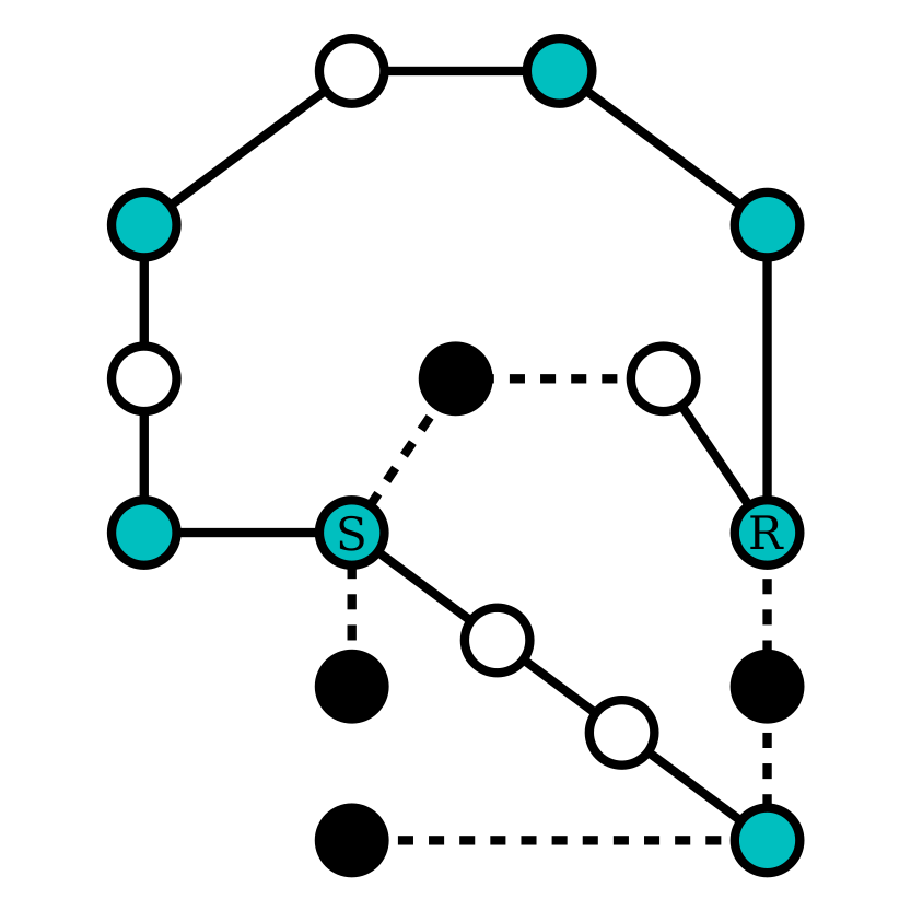
We consider a network in which there are many different design problems or other vulnerabilities, and each problem affects nodes of a different color $c$. This is illustrated in Fig. 1a with three colors (cyan, white and black). Assuming there are $n_{c}$ bad colors (colors white and black in the figure) and $m_{c}$ good colors (cyan in the figure), we might naively opt to restrict connectivity to good colored nodes only. However, this can render the entire system useless, if there are sufficiently many nodes with bad colors that their effective removal brings the network below the percolation threshold. For instance in Fig. 1a, assuming that black and white nodes are bad, nodes S and R cannot communicate using only cyan nodes and are effectively disconnected. Instead of just removing all of the bad colors, we can look for redundant paths where each path avoids one of the bad colors. As we can see in Fig. 1a, this can restore connectivity: Between nodes S and R there is a path avoiding black nodes (highlighted yellow) and a path avoiding white nodes (highlighted magenta). Because no single of the bad colors is required for connectivity, we can restore connectivity while remaining robust to the failure of any single color. Likewise, if the colors represent eavesdroppers and the message is split via secret sharing, and transmitted on multiple paths, no single eavesdropper can decode the whole message.

We define a pair of nodes as color-avoiding connected (CAC), if they have paths between them which avoid all of the vulnerable node colors, with each path avoiding a different node color. In the case that all of the colors are vulnerable, (as in [2]), that means that we require as many paths as colors (though not necessarily distinct). In Fig. 1a we see that there exist paths between sender S and receiver R avoiding only white nodes or avoiding only black nodes, and they are thus CAC. For color-avoiding percolation, we are interested in $\mathcal{L}_{\rm color}$, the maximal set of nodes which are CAC, and the conditions under which $\mathcal{L}_{\rm color}$ occupies a finite fraction of the total network. In [2], the theory of color-avoiding percolation was limited to the case in which every node was colored and all of the colors were trusted as senders/receivers. For transmission, the focus was on the case where all colors were avoided. A generalization with trusted colors for transmission was introduced, but the theory was not discussed in more detail. Here we generalize that theory to the case where arbitrary sets of colors are avoided or trusted as transmitters or as senders/receivers.

Assuming $C$ disjunctive sets of node colors with frequencies $r_{c}$ such that $\sum_{c=1}^{C}r_{c}=1$, we define the set of colors to be avoided as senders/receivers as $\mathcal{S}=\{s_{1},\dots,s_{R}\}\subseteq\{1,\dots,C\}$, and the set of colors to be avoided as transmitters as $\mathcal{T}=\{t_{1},\dots,t_{T}\}\subseteq\{1,\dots,C\}$. In Fig. 1a we have colors (1,2,3)=(blue,white,black), and we want to avoid white and black nodes for sending and transmitting: $\mathcal{S}=\mathcal{T}=\{{\rm white},{\rm black}\}$. If $\mathcal{S}=\mathcal{T}\neq\{1,\dots,C\}$, the node classes with colors in $\mathcal{T}$ are avoided for transmitting, and for sending and receiving as well. This can be used to represent the case, where certain node colors are universally mistrusted while other node colors are universally trusted. For instance, if a node of color $c$ is attempting to communicate with a node of color $c^{\prime}$, it may trust all nodes of its own color and the receiver color $c^{\prime}$ but not trust any other colors as either sender/receivers or transmitters. We return to this special case in detail in Sec. IV. For $\mathcal{S}=\emptyset$, nodes with problems are allowed to send or receive, while they are avoided for transmitting. This scenario is useful, if nodes of a class fail with a certain probability less than one. Or if the vulnerability of color $c$ does not impair the ability of the nodes to function as senders or receivers, but only impairs their transmitting abilities. In such a case, even though the sender itself has a vulnerable color, it still makes sense to avoid nodes of its own class on the path, in order to reduce the probability of disconnecting.

We define $\mathcal{C}_{\overline{c}}$ as the set of all nodes with color other than $c$, and $\mathcal{L}^{+}_{\overline{c}}$ as in [2]: We remove all nodes with color $c$ and find the largest component in the remaining graph, $\mathcal{L}_{\bar{c}}$. We then define $\mathcal{L}^{+}_{\bar{c}}$ as the set of all nodes which have a direct neighbour in $\mathcal{L}_{\bar{c}}$. This trivially includes the whole $\mathcal{L}_{\bar{c}}$ and additionally includes nodes of color $c$ that are directly connected to $\mathcal{L}_{\bar{c}}$ ($\mathcal{L}_{\overline{\rm white}}^{+}$ in Fig. 1b and $\mathcal{L}_{\overline{\rm black}}^{+}$ in Fig. 1c). These “dangling” $c$-colored nodes represent the nodes which can communicate via $\mathcal{L}_{\overline{c}}$, without requiring any $c$-colored nodes aside from themselves.

For the general case of avoiding a given set $\mathcal{S}$ of sender/receiver colors and a set $\mathcal{T}$ of transmitter colors, we find the color-avoiding giant component $\mathcal{L}_{\rm color}^{(\mathcal{S},\mathcal{T})}$ and its relative size $S_{\rm color}^{(\mathcal{S},\mathcal{T})}$ as

With $\neg\mathcal{L}^{+}_{\overline{t}}$ we refer to the network of nodes not belonging to $\mathcal{L}^{+}_{\overline{t}}$. Notice that negation turns the intersection into a union. The probability $S_{\rm color}^{(\mathcal{S},\mathcal{T})}$ describes the case where sending ($\mathcal{S}$) and transmitting ($\mathcal{T}$) nodes are avoided, and the probability $S_{\rm color}^{\mathcal{T}}$ describes the case where only transmitting nodes ($\mathcal{T}$) are avoided. In this manner, the giant color-avoiding component $S_{\rm color}$ defined in [2], can be obtained by letting $\mathcal{T}=\{1,\dots,C\}$ and $\mathcal{S}=\emptyset$, where all colors are avoided for transmitting, and no color is avoided for sending and receiving.

For Eq. 3, color distribution and connectivity properties are assumed to be independent. The first term in this equation describes a node property only, while the second term describes a property determined by connections and neighbors. We assume the colors to be distributed randomly, regardless of the network structure. This assumption has been verified with simulations, see for example Fig. 2. In order to use the formalism of generating functions, which are not well suited to unions of probabilities, we use the inclusion-exclusion principle [34] to rewrite

$\mathcal{Q}$ takes on all possible subsets of $\mathcal{T}$, including $\mathcal{T}$ itself, but not the empty set. The term $|\mathcal{Q}|$ denotes the number of elements in the set $\mathcal{Q}$ which is a subset of the set of avoided colors. In words, this equation uses the following rule: A sample is in the union of events, if it is in the first or second or third event etc., but double counting for pairwise intersections of events has to be subtracted. This procedure over-corrects intersections of triplets of events, which is then added back again and so on. We can now use single link probabilities and generating functions and rewrite

$u_{\mathcal{Q}}$ is the probability, that a node belongs to $\neg\mathcal{L}^{+}_{\overline{q}}$ for all colors $q\in\mathcal{Q}$, after we destroyed all of its links except for one randomly chosen link. In other words, it gives the probability that a node is not connected to any of the components $\mathcal{L}_{\overline{q}}$ ($q\in\mathcal{Q}$) over one particular link. The set $\mathcal{Q}$ is meant as an index of $u_{\mathcal{Q}}$, so we will use $u_{\{1,2\}}$ for $u_{\mathcal{Q}}$ with $\mathcal{Q}=\{1,2\}$, or $u_{\mathcal{T}}$ for $\mathcal{Q}=\mathcal{T}$ etc. In Eq. 6, we assume random ensembles of networks with size going to infinity and the locally treelike approximation. The probability for all links to fail to connect a certain node to components $\mathcal{L}_{\overline{q}}$ can be found with the generating function of the degree distribution $g_{0}$.

Finally, we need equations defining probabilities $u_{\mathcal{Q}}$. We use self consistency equations: A link fails to connect a first node with probability $u_{\mathcal{Q}}$, if the other node along this link is not connected to any of $\mathcal{L}_{\bar{q}}$ for $q\in\mathcal{Q}$, over any of its other links. For the first color the usual equation holds:

where $g_{1}(z)=g_{0}^{\prime}(z)/g_{0}^{\prime}(1)$ is the generating function of excess degree [17]. For two colors $c\neq q$ the equation reads

In equation 8, the first term represents the probability that the node reached through the link in question is of color $c$, and that at the same time it does not connect to the color avoiding component of color $q$. The second term represents the probability that the reached node is of color $q$, and that at the same time it does not connect to the color avoiding component of color $c$. The third term represents the probability that the reached node is neither of color $c$ nor $q$, but it also fails to connect to color avoiding components of colors $c$ and $q$ ( $L_{\overline{c}}$, $L_{\overline{q}}$). Clearly we have to plug in the result of the self consistent equations 7 into self consistent equation 8, to be able to compute the result. This has to be done numerically. In general, the equation for a joint probability that a node connects to none of the components avoiding colors $\mathcal{Q}$ over a particular link reads

where $\mathcal{Q}\setminus\{q\}$ is defined as the set containing all colors included in $\mathcal{Q}$, except for the color $q$. For capturing the case of only one color $\mathcal{Q}=\{c\}$, we define $u_{\emptyset}=1$, which is a consistent definition, as it is a solution of 9 itself ($u_{\emptyset}=g_{1}(u_{\emptyset})$). The only way to compute the joint probabilities for larger $|\mathcal{Q}|$ is to go step by step from joint probabilities for subsets of $\mathcal{Q^{\prime}}\in\mathcal{Q}$ using equation 9. In this way, all the subsets of $\mathcal{T}$ have to be considered, including $\mathcal{T}$ itself. The results have to be plugged into the equation for $S_{\rm color}^{\mathcal{T}}$. Combining equation 3 and the following equations up to equation 6 together, we find

Further using equation 9, this gives us the necessary input for calculating the size of the giant color avoiding component, equation 3. The comparison between this theory and the approximate theory developed in [2] is laid out in section 3.D.

In standard site percolation, the question is whether a large part of a network stays connected after a random fraction of nodes is destroyed. To demonstrate how the color-avoiding percolation framework can be described as a generalization of standard percolation, we consider the following color-avoiding percolation problem which is equivalent to standard percolation. We begin with a network composed of two node types: bad ($c=1$) and good ($c=2$). We assume the bad fraction is known to have design problems (as an extra property beyond the network connections), and therefore should be avoided for connections. Each color occurs with frequency $r_{c}$ such that $r_{1}+r_{2}=1$. With $S$ we denote the fraction of nodes in the surviving giant component, or equivalently, the probability for a single node to belong to the surviving giant component. That means, all nodes of the bad color $c=1$ are excluded as senders/receivers and as transmitters. We obtain:

Here we have assumed that $\mathcal{C}_{\overline{1}}$ and $\mathcal{L}^{+}_{\overline{1}}$ are independent, as discussed for color avoiding percolation above. It holds $P(\mathcal{C}_{\overline{1}})=1-r_{1}$. Equations 12 and 13 are convenient for calculations using the formalism based on generating functions [17, 35]. Assuming random ensembles of networks with size going to infinity and the locally treelike approximation, we further obtain

$P_{1{\rm link}}(\neg\mathcal{L}^{+}_{\overline{1}})$ is the probability, that a node belongs to $\neg\mathcal{L}^{+}_{\overline{1}}$, after we destroyed all of its links except for one randomly chosen link. In other words, it gives the probability that a node is not connected to the giant component over one particular link. These equations are equivalent to equations that describe random attack on networks [24, 23], as they should be.

To summarize the framework of color avoiding percolation, we found that $2^{|\mathcal{T}|}-1$ transcendental equations 9 have to be solved, to find $u_{\mathcal{Q}}$ for all subsets $\mathcal{Q}\subseteq\mathcal{T}$. Results are plugged into equation 10. For illustrating the procedure, let us discuss an example with three total colors, of which two are avoided for sending and transmitting: $C=3$, $\mathcal{S}=\mathcal{T}=\{1,2\}$.

For ten avoided colors, $1023$ subsets of $\mathcal{T}$ have to be considered, which is numerically still easy to do. If frequencies of all avoided colors are identical, the number of different transcendent equations reduces drastically to $|\mathcal{T}|$. However, for tens of avoided colors, the limited precision of numerical results for $u_{\mathcal{Q}}$ (especially due to the limited precision numerics for the generating function $g_{1}$) and the combination of many terms limits feasibility of the straight forward evaluation. In the general case of heterogeneous color frequencies, we observed that summing over the sets needed is an easy numerical task for our computer as long as $|\mathcal{T}|\leq 20$. For twenty avoided colors, about one million subsets have to be considered. We provide Python code in the appendix which works fast and precise enough for all examples discussed in the following (for 20 disjoint colors, it needs about a minute to calculate $S_{\rm color}^{\mathcal{T}}$ on one core of an Intel® Core™ i7-4770 CPU (3.40GHz)), even if there is still much room for optimization. Below we discuss an approximation for reducing the number of colors, if many color frequencies are small compared to the largest color frequency.

The critical behavior of color avoiding percolation has a rich, multifaceted nature, depending on graph topology, number of avoided colors and color frequencies. We will discuss a number of phenomena using special cases below. However, the transition point can be understood within the general theory framework, by referencing standard percolation. Without loss of generality, we assume for the avoided colors $\mathcal{T}=\{1,2,\dots,T\}$, and the total frequency of color $c=1$, $r_{1}$, is larger or equal compared to the frequencies of all other avoided colors. We have for $c\in\mathcal{T}$: $u_{\{c\}}=r_{c}+\left(1-r_{c}\right)g_{1}(u_{\{c\}})$. From standard percolation we know, that if color $c=1$ can be avoided ($u_{\{1\}}<1$), then this is true for all other avoided colors as well, as they have smaller frequencies. Accordingly, color $c=1$ is the first to have vanishing connectivity, $u_{\{1\}}=1$. In this latter case, we have $S_{\rm color}^{(\mathcal{S},\mathcal{T})}=0$, as all terms $g_{1}(u_{\mathcal{Q}})$ in equation 10 cancel out pairwise. First this is true for $1-g_{1}(u_{\{1\}})$. Equation 9 for $u_{\{1,2\}}$ reduces with $g_{1}(u_{\{1\}})=1$ to the defining equation for $u_{\{2\}}$, thus $g_{1}(u_{\{1,2\}})-g_{1}(u_{\{2\}})=0$. This generalizes to $u_{\mathcal{Q}}=u_{\mathcal{Q}\cup\{1\}}$. Accordingly, the critical point is determined by the avoided color with the largest frequency, in the same way as for standard percolation. With the result of Cohen [23] we find as a condition for non-vanishing connectivity (with expected degree $\bar{k}$)

The probabilities $u_{\mathcal{Q}}$ are hard to interpret, as they describe a negative statement: The probability of a link to not connect to several $\mathcal{L}_{\bar{c}}$ at the same time. This makes it confusing to discuss the meaning of dependencies, for example in the form $u_{\{1,2\}}\neq u_{\{1\}}u_{\{2\}}$. Furthermore, it turns out that for larger sets $\mathcal{Q}$ with more than one element, it is hard to find good approximations for $u_{\mathcal{Q}}$. This complicates understanding the critical behavior. Therefore, let us define new positive variables, describing the probability that a link connects to all $\mathcal{L}_{\overline{q}}$ for $q\in Q$ at the same time:

The conditions between $u_{\mathcal{Q}}$ and $v_{\mathcal{Q}}$ hold with the complementary event and the inclusion-exclusion principle. As the transformation from $u_{\mathcal{Q}}$ to $v_{\mathcal{Q}}$ can be reversed with the same transformation (it is an involution), and it preserves all information, variables $v_{\mathcal{Q}}$ are dual variables to $u_{\mathcal{Q}}$. If probabilities were independent, to connect to several $\mathcal{L}_{\overline{q}}$ for $q\in Q$ at the same time over the same link, it would hold $v_{\mathcal{Q}}=\prod_{q\in\mathcal{Q}}v_{\{q\}}$. As we will discuss below, conditional probabilities for further colors can both be suppressed and increased.

It is useful to have equations for calculating $v_{\mathcal{Q}}$ directly, instead of first calculating $u_{\mathcal{Q}}$ and then transforming to $v_{\mathcal{Q}}$. Approximations are easier found for calculating $v_{\mathcal{Q}}$ directly. For $\mathcal{Q}\neq\{1,\dots,C\}$ it holds:

In the first of these equations, only $u_{\mathcal{Q}}$ was plugged in using equation 20. Equation 22 can be understood as follows: Starting with $\mathcal{Q}=\{c\}$, replace the left hand side of Eq. 9 using Eq. 20, and solve for $g_{1}(u_{\{c\}})$. For increasing from $\mathcal{Q}\setminus{\{q\}}$ to $\mathcal{Q}$, replace the left hand side of Eq. 9 using Eq. 20. Then plug in the lower order results already obtained to the right hand side of equation 9, and solve for $g_{1}(u_{\mathcal{Q}})$. Finally, it holds

This reflects the fact that a single link can never be used for avoiding all colors at the same time. The node reached over this link has a certain color, consequently this color cannot be avoided.

For Poisson graphs, the conditions for critical parameters read

and solving for $\bar{k}$, we have

Critical behavior according to varying topology or varying color frequencies is, as usual, described using the critical exponent $\beta$. For clarity we use two exponents:

This can be dominated by the avoided color with the largest frequency, but in general the interplay of different colors can lead to new effects which are not present in standard percolation.

The critical behavior of color avoiding percolation shows interesting features, as we see in Fig. 2c. While the phase transition along the dashed white lines has critical exponent $\beta_{k}=\beta_{r}=1$, the situation is different, along the dotted white line, with $\beta_{k}=2$. The behavior of $\beta_{k}$ can be summarized as follows: The critical exponent $\beta_{k}$ is determined by the degeneracy of the maximal color frequency, i.e., the number of colors which are tied for most common,

Below we will confirm this result using an approximate scheme, explicitly presenting results for up to three avoided colors. In [2] it was reported that $\beta_{k}=C$, under the assumption that all $C$ colors are avoided for transmission, and they all have the same frequency. The more detailed analysis here confirms these results and shows the correct extension to cases where the colors have different frequencies.

The increased critical exponent $\beta_{k}=2$ along the dotted line in Fig. 2c is connected to a sharp bend in the critical manifold, shown with a straight white line. It also is connected to the fact, that color connectivity is most suppressed compared to only avoiding the dominant color, if $r_{1}=r_{2}$ (see (b)). Between both kinds of phase transition, with $\beta_{k}=1$ and $\beta_{k}=2$, there has to be some kind of crossover. This is important to understand in order to determine the behavior of finite size networks with $r_{1}\approx r_{2}$. Before we turn to an analytic examination of $S_{\rm color}$ in the crossover regime, let us discuss the phenomenology with figure 3. We use logarithmic scaling on both axis, thus power law dependencies show as straight lines. We set $r_{1}=0.2$ for the avoided color with the largest frequency, in order to keep $\bar{k}_{\rm crit}$ fixed. Results are shown with straight lines for the cases $r_{2}=r_{1}$ (red line), $r_{2}=r_{1}-0.03$ (green line), $r_{2}=r_{1}/2$ (black line) and $r_{2}=0$ (blue line). Numerical results are in good agreement with the theory, only limited by finite size effects for small size of the largest CAC component. If the frequency of the second color is far below the frequency of the first color (black line), we see that color connectivity is overall reduced compared to one avoided color (blue line), but the critical behavior is not affected. If the frequency of the second color is close to that of the first color (green line), the behavior is close to this with identical color frequencies for large connectivity (red line). Therefore, the increased critical exponent $\beta_{k}=2$ is of practical relevance in finite size graphs, if color frequencies are close to each other. Closer to the critical point, the deviation of color frequencies results in a critical exponent of $\beta_{k}=1$.

For small deviations of color frequencies $r_{1}\approx r_{2}$ (and $r_{1}\geq r_{2})$, we can analyze the critical behavior analytically. We start with one avoided color. It is well known, that for Poisson graphs the critical exponent of standard percolation is $\beta_{k}=1$. We reproduce this result using the alternative formulation Eq. 22 with an expansion of the generating function for small $v_{\{c\}}$ ($c=1,2$). $v_{\mathcal{Q}}$ replaces $u_{\mathcal{Q}}$ as defined in Eq. 19. We have

We define $\bar{k}_{c}=1/(1-r_{c})$. For $\bar{k}<\bar{k}_{1}=\bar{k}_{\rm crit}$ we have $v_{\{1\}}=0$. With Eq. 24 we have $S_{\rm color}^{(\{1\},\{1\})}=v_{\{1\}}$, and therefore we found $\beta_{k}=1$. How does the critical behavior generalize to two colors, $v_{\{1,2\}}$? Still, color $c=1$ is the color with higher frequency, and the critical behavior is connected to small $v_{\{1\}}$, increasing from zero. As we are interested in color frequencies with small deviation, we assume small $v_{\{2\}}$ as well. We develop the self consistency equation 22 accordingly,

Most of the terms canceled out with approximate results for $v_{\{1\}}$ and $v_{\{2\}}$ from above. The largest correction in Eq. 35 is of order $v_{\{1\}}v_{\{2\}}^{2}$, therefore the approximation requires $v_{\{2\}}\ll 1$. With $\bar{k}_{1}\approx\bar{k}_{2}$ and $S_{\rm color}^{(\mathcal{T},\mathcal{T})}=v_{\mathcal{T}}$, we find that color connectivity scales with $(\bar{k}-\bar{k}_{\rm crit})^{2}$, as long as $(\bar{k}-\bar{k}_{\rm crit})\gg(\bar{k}_{1}-\bar{k}_{2})$. For $r_{1}=r_{2}$, we thus find $\beta_{k}=2$. For $r_{1}>r_{2}$, the critical exponent $\beta_{k}=1$ is only visible for $(\bar{k}-\bar{k}_{\rm crit})\ll(\bar{k}_{1}-\bar{k}_{2})$, what can be dominated by finite size effects, if color frequencies are close to each other.

With three avoided colors, we can analyze how the critical behavior generalizes to more colors. Figure 4 shows results for disjoint colors on Poisson graphs, where three colors are avoided. We fix the frequency of the first color to $r_{1}=0.3$. Again, $S_{\rm color}^{\{1,2,3\}}$ can be seen as the fraction of nodes in the largest CAC component, among all nodes of color four. Compared to the black line, showing results where the other frequencies of avoided colors are smaller ($r_{2}=r_{3}=0.12$, $r_{4}=0.46$), degeneration of the highest avoided color frequency reduces color connectivity considerably. The results shown in (a) are repeated in (b) with logarithmic scaling, to demonstrate the critical power law behavior. The blue line shows results for double degenerate highest frequency $r_{1}=r_{2}=0.3$, and the exponent increases to $\beta_{k}=2$. We saw this exponent already for two avoided colors with degenerated frequencies. Now we see, that with a third avoided color with smaller frequency $r_{3}=0.12$, the exponent stays the same. The crossover as described for two avoided colors applies here as well, and the two-dimensional critical manifold in the parameter space $(r_{1},r_{2},r_{3})$ has a sharp bend as well (results not shown). The red line shows results for triple degenerate highest color frequency of avoided colors $r_{1}=r_{2}=r_{3}$. This is connected with critical exponent $\beta_{k}=3$. This exponent can be extracted analytically, in the same way as it was done for two avoided colors. Using $v_{\{1\}}=v_{\{2\}}$ etc. for identical frequencies of avoided colors, we develop Eq. 33 to third order (instead of second order), plug into an equation 22 for $g_{1}(u_{\{1,2,3\}})$, develop to third order and solve the leading terms for $v_{\{1,2,3\}}$:

where we have used the fact that $v_{\{1\}}\sim(\overline{k}-\overline{k}_{\rm crit})$ from Eq. 32 and $v_{\{1,2\}}\sim(\overline{k}-\overline{k}_{\rm crit})^{2}$ from Eq. 36. A similar procedure can be applied for higher numbers of avoided colors and heterogeneous color frequencies, which would require higher order expansions in the generating functions, and many terms of same order to be considered. The only case, in which this procedure is not applicable, is for avoiding all colors for transmission. It holds $v_{\{1,\dots,C\}}=0$, while $S_{\rm color}$ is finite. For this case, the approximation of [2] can be useful, as discussed in the section about approximations.

Here we consider the probability of a link simultaneously avoiding all colors in a set $\mathcal{Q}$, or in other words simultaneously connecting to all sets $\mathcal{L}_{\bar{c}}$ for the colors $c\in\mathcal{Q}$. This probability is calculated exactly in equation (19) and is related directly to the overall connectivity (Eq. (24)). When considering the phase transition, we found that this probability is proportional to the product of probabilities for each color $c\in\mathcal{Q}$ separately. Although these probabilities are not independent, we found above that the critical point and scaling exponent are consistent with the assumption that they are independent (cf. equation (35)). To understand what impact the dependencies between colors have on the overall color-avoiding connectivity, we compare the assumption that the connections are independent for different colors with the full solution obtained above. We define the assumption of independent probabilities (AIP) by taking

As we found for Poisson graphs $S_{\rm color}^{(\mathcal{S},\mathcal{T})}\propto v_{\mathcal{T}}$, this can help us to understand the critical behavior. Apart from that, comparing $v_{\mathcal{Q}}^{\rm AIP}$ with results $v_{\mathcal{Q}}$, where all dependencies are explicitly included, can teach us about dependencies.

In Fig. 5a we see that for two avoided colors with different frequencies, $v_{\mathcal{T}}$ and $v_{\mathcal{T}}^{\rm AIP}$ have the same qualitative behavior. This way, the critical exponent $\beta_{k}$ can be understood as follows: The probability $v_{\{1\}}$ for avoiding a first color has a linear onset starting from the critical point. As the probability $v_{\{2\}}$ already has reached a positive value, the probability for both at the same time has a linear onset as well. With Eq. 35, we can estimate dependencies close to the critical point (as long as $v_{\{2\}}\ll 1$) to be

We find that the conditional probability that the same link helps to avoid a second color can be increased as compared to the probability for the first color (as in the figure close to the critical point). The conditional probability can also be suppressed (in the figure for large $\bar{k}$, or for $r_{1}=0.45$ and $r_{2}=0.4$ in the whole regime of $\bar{k}$, results not shown). In Fig. 5b we see how $v_{\mathcal{Q}}^{\rm AIP}$ can help to understand larger critical exponents for degenerated largest color frequencies.

If all colors are avoided, we always have $v_{\{1,\dots,C\}}=0<v_{\{1,\dots,C\}}^{\rm AIP}$. This reflects the fact that in this case no single link can be used to avoid all colors, as the node reached over the link in question has one color, which cannot be avoided. Accordingly, only nodes in the two-core can be in the giant CAC component [2]. This is in line with our analysis of the limit where $C\rightarrow\infty(N)$ [2]. There we showed that, rather than recovering standard percolation in this case, we instead recover $k$-core percolation with $k=2$ [10, 11, 36]. On the other hand, color connectivity can be expressed in terms of variables $v_{\mathcal{Q}}$ using Eq. 10 and 20. In Sec. V we discuss that the condition $v_{\{1,\dots,C\}}=0$ must be fulfilled by any appropriate approximation for color avoiding percolation, and how this helps for the heuristic approximation of [2].

In order to compare with the approximate results presented in [2], we avoid all $C$ colors for transmission and none for sending. All colors have identical frequencies $r_{c}=r_{1}=1/C$. We have $u_{\{c,q\}}=u_{\{1,2\}}$ etc. We can simplify

This reduces the number of quantities $u_{\mathcal{Q}}$ to be calculated from $2^{C}-1$ to $C$. This only reduces the computation time, as there are still numerical problems. Combinatorial factors ${C\choose j}$ are large for large $C$, and results for $u_{\{1,2,\dots,j\}}$ can only be numerical, with limited precision. Especially limited precision for calculating the generating functions causes problems for small $S_{\rm color}$.

In [2], $u_{\{1,2,\dots,j\}}$ was estimated using the approximation

$u$ is the probability that a node is not connected to the giant component over one particular link and is computed as the solution of $u=g_{1}(u)$, where $g_{1}(z)=g_{0}^{\prime}(z)/g_{0}^{\prime}(1)$ is the generating function of excess degree [17]. $U_{\{1\}}$ denotes the conditional probability that a link fails to connect to $\mathcal{L}_{\bar{1}}$ given that it does connect to the normal giant component via a node having a color $c\neq 1$. We define $U_{\{1\}}=1$ if $u=1$. The probability $u_{\{1\}}$ that a single link does not connect to a giant $\mathcal{L}_{\bar{1}}$ is calculated with Eq. 7.

The approximation for $u_{\{1,\dots,j\}}$ is motivated as follows: With probability $u$ a link does not connect to the giant component, so $u_{\{1,\dots,j\}}\geq u$. If it connects to the giant component (probability $(1-u)$), then the node on the other side has either one of the $j$ colors (probability $j/C$), leaving simultaneous failure probability of $(U_{\{1\}})^{j-1}$, or it has a different color with probability $(C-j)/C$, leaving simultaneous failure probability of $(U_{\{1\}})^{j}$. In this approximation, we neglect dependencies among the conditional probabilities $U_{\{1\}},U_{\{2\}}$ etc. Therefore, we call this approximation in the following as the approximation of independent conditional probabilities (AICP).

A comparison of AICP and the theory presented here is shown in Fig. 8. We see that for $C=3$ colors AICP works well (upper panel). For as many as $C=10$ colors, results are still good for large $S_{\rm color}$, while for $S_{\rm color}<10^{-2}$ there are strong deviations between the theory presented here and AICP. However, the critical behavior in terms of the critical point $\bar{k}_{\rm crit}$, and the fact that the critical exponent $\beta_{k}$ is large, are still captured.

In order to understand AICP better, let us define

In Fig. 9 on the right, $\delta_{5}^{\rm AICP}$ is shown with a red solid line, for $C=5$. We see that $\delta_{5}^{\rm AICP}$ is a quadratic function in $\bar{k}-\bar{k}_{\rm crit}$ for small values of this variable, therefore $u_{\{1,\dots,C\}}^{\rm AICP}$ behaves like a linear expansion around the critical point. This is true for $j<C$ as well (results not shown). However, final results for $S_{\rm color}$ as shown on the left of the figure (black line for the theory, red dashed line for AICP) are compatible with an exponent $\beta_{k}=C=5$. To understand better, how a linear expansion in $\bar{k}-\bar{k}_{\rm crit}$ of variables $u_{\{1,\dots,j\}}$ can finally reproduce such a steep critical behavior, let us discuss the constraints

The first of these equations represents the fact that a node can never be CAC via a single link, if no color is trusted. This constraint is also respected with AICP: In [2] it was shown that the largest CAC is always a subset of the 2-core. This constraint also implies that $S_{\rm color}$, as calculated with equation 10, cannot easily be truncated after terms with a certain $|\mathcal{Q}|=Q_{\rm truncate}$. To show that the constraint equation 49 is crucial for AICP, let us define a fake approximation denoted as “app1”, which is closer to the theory, but violates the constraint. We set

$\delta_{5}^{\rm app1}$ is shown with a green solid line in the right panel of the figure. As $\delta_{j}^{\rm AICP}\ll 1$ for all $j$, $u_{\{1,\dots,j\}}^{\rm app1}$ is a slightly better approximation of the variables $u_{\{1,\dots,j\}}$. However, the resulting $S_{\rm color}^{\rm app1}$ fails to describe the critical behavior of $S_{\rm color}$, as shown on the left of the figure with a solid green line. Instead we find a result compatible with $S_{\rm color}^{\rm app1}\propto(\bar{k}-\bar{k}_{\rm crit})^{2}$, what reflects the fact that we have a linear expansion in $\bar{k}-\bar{k}_{\rm crit}$. Indeed, the result is dominated by

shown on the left of the figure with a dashed green line. If the constraint would be fulfilled, this residual would be zero.

With the last subsection we saw that the equations defining $S_{\rm color}$ as presented in this paper are hard to approximate. On the other hand, the complexity for homogeneous color frequencies grows exponentially with the number of avoided colors (for transmission). If there is a large number of colors with marginal frequencies, we can use the theory as presented in this paper, and manipulate the set of avoided colors, or combine all colors with small frequencies to one color. As can be seen in Fig. 10, this allows to give upper and lower bounds to $S_{\rm color}$.

References

- [1] Dirk Helbing, “Globally networked risks and how to respond,” Nature 497, 51–59 (2013).
- [2] Sebastian M. Krause, Michael M. Danziger, and Vinko Zlatić, “Hidden connectivity in networks with vulnerable classes of nodes,” Phys. Rev. X 6, 041022 (2016).
- [3] Ronald W Ritchey and Paul Ammann, “Using model checking to analyze network vulnerabilities,” in Security and Privacy, 2000. S&P 2000. Proceedings. 2000 IEEE Symposium on (IEEE, 2000) pp. 156–165.
- [4] Kim-Kwang Raymond Choo, “Cloud computing: challenges and future directions,” Trends and Issues in Crime and Criminal justice , 1 (2010).
- [5] P. Trkman, M.I. Štemberger, J. Jaklič, and A. Groznik, “Process approach to supply chain integration,” Supply Chain Management 12, 116–128 (2007).
- [6] S. Li, S.S. Rao, T.S. Ragu-Nathan, and B. Ragu-Nathan, “Development and validation of a measurement instrument for studying supply chain management practices,” Journal of Operations Management 23, 618–641 (2005).
- [7] Peter Trkman and Kevin McCormack, “Supply chain risk in turbulent environments—A conceptual model for managing supply chain network risk,” International Journal of Production Economics 119, 247–258 (2009).
- [8] Danny Dolev, Cynthia Dwork, Orli Waarts, and Moti Yung, “Perfectly secure message transmission,” J. ACM 40, 17–47 (1993).
- [9] Jorg Stelling, Uwe Sauer, Zoltan Szallasi, Francis J. Doyle III, and John Doyle, “Robustness of cellular functions,” Cell 118, 675 – 685 (2004).
- [10] S. N. Dorogovtsev, A. V. Goltsev, and J. F. F. Mendes, “-core organization of complex networks,” Phys. Rev. Lett. 96, 040601 (2006).
- [11] A. V. Goltsev, S. N. Dorogovtsev, and J. F. F. Mendes, “-core (bootstrap) percolation on complex networks: Critical phenomena and nonlocal effects,” Phys. Rev. E 73, 056101 (2006).
- [12] Shai Carmi, Shlomo Havlin, Scott Kirkpatrick, Yuval Shavitt, and Eran Shir, “A model of internet topology using k-shell decomposition,” Proceedings of the National Academy of Sciences 104, 11150–11154 (2007).
- [13] M. E. J. Newman and Gourab Ghoshal, “Bicomponents and the robustness of networks to failure,” Phys. Rev. Lett. 100, 138701 (2008).
- [14] Marjan Radi, Behnam Dezfouli, Kamalrulnizam Abu Bakar, and Malrey Lee, “Multipath routing in wireless sensor networks: Survey and research challenges,” Sensors 12, 650–685 (2012).
- [15] Chi Ho Yeung, David Saad, and KY Michael Wong, “From the physics of interacting polymers to optimizing routes on the london underground,” Proceedings of the National Academy of Sciences 110, 13717–13722 (2013).
- [16] R. Cohen and S. Havlin, Complex Networks: Structure, Robustness and Function (Cambridge University Press, 2010).
- [17] Mark Newman, Networks: an introduction (OUP Oxford, 2010).
- [18] Flaviano Morone and Hernán A. Makse, “Influence maximization in complex networks through optimal percolation,” Nature 524, 65–68 (2015).
- [19] Tiago P. Peixoto and Stefan Bornholdt, “Evolution of robust network topologies: Emergence of central backbones,” Phys. Rev. Lett. 109, 118703 (2012).
- [20] Byungjoon Min, Su Do Yi, Kyu-Min Lee, and K.-I. Goh, “Network robustness of multiplex networks with interlayer degree correlations,” Phys. Rev. E 89, 042811 (2014).
- [21] Vinko Zlatić, Diego Garlaschelli, and Guido Caldarelli, “Networks with arbitrary edge multiplicities,” EPL (Europhysics Letters) 97, 28005 (2012).
- [22] Davide Cellai, Sergey N. Dorogovtsev, and Ginestra Bianconi, “Message passing theory for percolation models on multiplex networks with link overlap,” Phys. Rev. E 94, 032301 (2016).
- [23] Reuven Cohen, Keren Erez, Daniel Ben-Avraham, and Shlomo Havlin, “Resilience of the internet to random breakdowns,” Physical review letters 85, 4626 (2000).
- [24] Duncan S Callaway, Mark EJ Newman, Steven H Strogatz, and Duncan J Watts, “Network robustness and fragility: Percolation on random graphs,” Physical review letters 85, 5468 (2000).
- [25] Jianxi Gao, Sergey V. Buldyrev, Shlomo Havlin, and H. Eugene Stanley, “Robustness of a Network of Networks,” Phys. Rev. Lett. 107, 195701 (2011).
- [26] Michael M. Danziger, Louis M. Shekhtman, Amir Bashan, Yehiel Berezin, and Shlomo Havlin, “Vulnerability of interdependent networks and networks of networks,” in Interconnected Networks, edited by Antonios Garas (Springer International Publishing, Cham, 2016) pp. 79–99.
- [27] P. Grassberger, “On the critical behavior of the general epidemic process and dynamical percolation,” Mathematical Biosciences 63, 157 – 172 (1983).
- [28] M. E. J. Newman, “Spread of epidemic disease on networks,” Phys. Rev. E 66, 016128 (2002).
- [29] Romualdo Pastor-Satorras and Alessandro Vespignani, “Epidemic spreading in scale-free networks,” Phys. Rev. Lett. 86, 3200–3203 (2001).
- [30] M Angeles Serrano and Marián Boguná, “Percolation and epidemic thresholds in clustered networks,” Physical review letters 97, 88701 (2006).
- [31] J Goldenberg, B Libai, S Solomon, N Jan, and D Stauffer, “Marketing percolation,” Physica A: Statistical Mechanics and its Applications 284, 335 – 347 (2000).
- [32] Daniel R Wuellner, Soumen Roy, and Raissa M D’Souza, “Resilience and rewiring of the passenger airline networks in the united states,” Physical Review E 82, 056101 (2010).
- [33] Daqing Li, Bowen Fu, Yunpeng Wang, Guangquan Lu, Yehiel Berezin, H. Eugene Stanley, and Shlomo Havlin, “Percolation transition in dynamical traffic network with evolving critical bottlenecks,” Proceedings of the National Academy of Sciences 112, 669–672 (2015).
- [34] Charles M. Grinstead and Laurie J. Snell, Introduction to Probability, version dated 4 july 2006 ed. (American Mathematical Society, 2006).
- [35] Mark EJ Newman, Steven H Strogatz, and Duncan J Watts, “Random graphs with arbitrary degree distributions and their applications,” Physical Review E 64, 026118 (2001).
- [36] D. Lee, M. Jo, and B. Kahng, “Critical behavior of -core percolation: Numerical studies,” ArXiv e-prints (2016), arXiv:1609.07275 [cond-mat.stat-mech] .