A Bayesian optimization approach to find Nash equilibria

We consider primarily the standard (static, under complete information) Nash equilibrium problem (Gibbons, 1992, NEP,).

Each block $\mathbf{x}_{i}$ denotes the variables of player $i$ and $\mathbb{X}_{i}$ its corresponding action space and $\mathbb{X}=\prod_{i}\mathbb{X}_{i}$. We shall use the convention $y_{i}(\mathbf{x})=y_{i}(\mathbf{x}_{i},\mathbf{x}_{-i})$ when we need to emphasize the role of $\mathbf{x}_{i}$.

In other words, when all players have chosen to play a NE, then no single player has incentive to move from his $\mathbf{x}^{*}_{i}$. Let us however mention by now that, generically, Nash equilibria are not efficient, i.e., do not belong to the underlying set of best compromise solutions, called Pareto front, of the objective vector $(y_{i}(\mathbf{x}))_{\mathbf{x}\in\mathbb{X}}$.

We shall also deal with the case where cost functions are uncertain. Such problems belong to a family of random games that are called disturbed games by Harsanyi in (Harsanyi, 1973). We denote such cost functions $f_{i}(\mathbf{x},\bm{\epsilon}(\xi))$, where $\bm{\epsilon}=(\epsilon_{i}):\Xi\rightarrow\mathbb{R}^{p}$ is a random vector defined over a probability space $(\Xi,\mathcal{F},\mathbb{P})$. In the following we refer to our setting as random games, but emphasize that we consider static Nash games with expectations of randomly perturbed costs.

Note that setting $y_{i}=\mathbb{E}[f_{i}(\mathbf{x},\bm{\epsilon}(\xi))]$, we see directly that $(NE)$ and $(SNE)$ are equivalent.

In this work, we focus on continuous-strategy non-cooperative Nash games (i.e., with infinite sets $\mathbb{X}_{i}$) or on large finite games (i.e., with large finite sets $\mathbb{X}_{i}$).

Our working hypotheses are:

• •

  queries on the cost function (i.e., pointwise evaluation of the $y_{i}$’s for a given $\mathbf{x}$) result from an expensive process: typically, the $y_{i}$’s can be the outputs of numerical models;

• •

  the cost functions may have some regularity properties but are possibly strongly not convex (e.g., continuous and multimodal);

• •

  the cost functions evaluations can be corrupted by noise;

• •

  $\mathbb{X}$ is either originally discrete, or a representative discretization of it is available (so that the equilibrium of the corresponding finite game is similar to the one of original problem).

Note that to account for the particular form of NEPs, $\mathbb{X}$ must realize a full-factorial design: $\mathbb{X}=\mathbb{X}_{1}\times\ldots\times\mathbb{X}_{p}$. Given each action space $\mathbb{X}_{i}=\{\mathbf{x}_{i}^{1},\ldots,\mathbf{x}_{i}^{m_{i}}\}$ of size $m_{i}$, $\mathbb{X}$ consists of all the combinations $(\mathbf{x}_{i}^{k},\mathbf{x}_{j}^{l})$ ($1\leq i\neq j\leq p$, $1\leq k\leq m_{i}$, $1\leq l\leq m_{j}$), and we have $N:=\operatorname{Card}(\mathbb{X})=\prod_{i=1}^{p}m_{i}$.

Let us remark that we do not require for an equilibrium to exist and be unique, the case when there is no or equilibria is discussed in Section 3.2.4.

In the case of noisy evaluations, we consider only here an additive noise corruption:

and we assume further that $\bm{\epsilon}$ has independent Gaussian centered elements: $\epsilon_{i}\sim\mathcal{N}(0,\tau_{i}^{2})$. Notice that in this case, both problems and equilibria coincide, and can be solved with the same algorithm. Hence, in the following, all calculations are given in the noisy case, while the deterministic case of the standard NEP is recovered by setting $\epsilon_{i}=0$ and $\tau_{i}=0$.

Furthermore, we consider solely pure-strategy Nash equilibria (as opposed to mixed-strategies equilibria, in which the optimal strategies can be chosen stochastically, see Gibbons, 1992, Chapter 1), and as such, we avoid solving the linear programs LP or linear complementarity problems LCP generally used in the dedicated classes of algorithms à la Lemke-Howson (Rosenmüller, 1971).

Let us mention that in the continuous (in the sense of smooth) games setting, there is an extensive literature dedicated to the computation of NE, based on the rich theory of variational analysis, starting with the classical fixed-point algorithms to solve NEPs (Uryas’ev & Rubinstein, 1994; Başar, 1987; Li & Başar, 1987). When the players share common constraints, Nash equilibria are shown to be Fritz-John (FJ) points (Dorsch et al., 2013), which allows the op. cit. authors to propose a nonsmooth projection method (NPM) well adapted for the computation of FJ points. From other part, it is well known (and straightforward) that Nash equilibria are in general not classical Karush-Kuhn-Tucker (KKT) points, nevertheless, a notion of KKT condition for generalized Nash equilibria GNEP is developed in Kanzow & Steck (2016), which allows the authors to derive an augmented Lagrangian method to compute GNEPs.

Noncooperative stochastic games theory, starting from the seminal paper by Shapley (Shapley, 1953), occupies nowadays most of the game theorists, and a vast literature is dedicated to stochastic differential games (Friedman, 1972), robust games (Nishimura et al., 2009), games on random graphs, or agents learning games (Hu & Wellman, 2003), among many other branches, and it is definitely out of the scope of the paper to review all aspects of the field. See also the introductory book Neyman & Sorin (2003) to the basic -yet deep- concepts of the stochastic games theory.

We also do not consider games with additional specific structures, like cooperative, zero-sum stochastic or deterministic games, or repeated Nash games (Littman & Stone, 2005). For these games, tailored algorithms should be used, among which are the pure exploration statistical learning with Monte Carlo Tree Search (Garivier et al., 2016) or multi-agent reinforcement learning MARL, see e.g., Games (2016) and references therein.

We stress here that none of the above-mentioned approaches are designed to tackle expensive black-box problems. They may even prove unusable in this context, either because they could simply not converge or require too many cost function evaluations to do so.

The idea of replacing an expensive function by a cheap-to-evaluate surrogate is not recent, with initial attempts based on linear regression. Gaussian process (GP) regression, or kriging, extends the versatility and efficiency of surrogate-based methods in many applications, such as in optimization or reliability analysis. Among alternative non-parametric models such as radial basis functions or random forests, see e.g., Wang & Shan (2007); Shahriari et al. (2016) for a discussion, GPs are attractive in particular for their tractability, since they are simply characterized by their mean $m$ and covariance (or kernel) $k$ functions, see e.g., Cressie (1993); Rasmussen & Williams (2006). In the following, we consider zero-mean processes ($m=0$) for the sake of conciseness.

Briefly, for a single objective $y$, conditionally on $n$ noisy observations $\mathbf{f}=(f_{1},\ldots,f_{n})$, with independent, centered, Gaussian noise, that is, $f_{i}=y(\mathbf{x}_{i})+\varepsilon_{i}$ with $\varepsilon_{i}\sim\mathcal{N}(0,\tau_{i}^{2})$, the predictive distribution of $y$ is another GP, with mean and covariance functions given by:

where $\textbf{k}(\mathbf{x}):=(k(\mathbf{x},\mathbf{x}_{1}),\dots,k(\mathbf{x},\mathbf{x}_{n}))^{\top}$ and $\textbf{K}:=(k(\mathbf{x}_{i},\mathbf{x}_{j})+\tau_{i}^{2}\delta_{i=j})_{1\leq i,j\leq n}$, $\delta$ standing for the Kronecker function. Commonly, $k$ belongs to a parametric family of covariance functions such as the Gaussian and Matérn kernels, based on hypotheses about the smoothness of $y$. Corresponding hyperparameters are often obtained as maximum likelihood estimates, see e.g., Rasmussen & Williams (2006) or Roustant et al. (2012) for the corresponding details.

With several objectives, a statistical emulator for $\mathbf{y}(\mathbf{x})=\left[y_{1}(\mathbf{x}),\ldots,y_{p}(\mathbf{x})\right]$ is needed. While a joint modeling is possible (Álvarez et al., 2011, see e.g.,), it is more common practice to treat the $y_{i}$’s separately. Hence, conditioned on a set of vectorial observations $\{\mathbf{f}_{1},\ldots,\mathbf{f}_{n}\}$, our emulator is a multivariate Gaussian process $\mathbf{Y}$:

with $\bm{\mu}(.)=\left[\mu_{1}(.),\dots,\mu_{p}(.)\right]$, $\bm{\Sigma}=\operatorname{diag}\left(\sigma_{1}^{2}(.,.),\ldots,\sigma_{p}^{2}(.,.)\right)$, such that $\{\mu_{i}(.),\sigma_{i}^{2}(.,.)\}$ is the predictive mean and covariance, respectively, of a GP model of the objective $y_{i}$. Note that the predictive distribution of an observation is:

GPs are commonly limited to a few thousands of design points, due to the cubic cost needed to invert the covariance matrix. This can be overcome in several ways, by using inducing points Wilson & Nickisch (2015), or local models Gramacy & Apley (2015); Rullière et al. (2016); see also Heaton et al. (2017) for a comparison or Žilinskas & Zhigljavsky (2016) for a broader discussion. In addition, here the full-factorial structure of the design space can potentially be exploited. For instance, if evaluated points also have a full-factorial structure, then the covariance matrix can be written as a Kronecker product, reducing drastically the computational cost, see e.g., Plumlee (2014).

Bayesian optimization methods are usually outlined as follows: a first set of observations $\{\mathbf{X}_{n_{0}},\mathbf{f}_{n_{0}}\}$ is generated using a space-filling design to obtain a first predictive distribution of $\mathbf{Y}(.)$. Then, observations are performed sequentially by maximizing a so-called acquisition function (or infill criterion) $J(\mathbf{x})$, that represents the potential usefulness of a given input $\mathbf{x}$. That is, at step $n\geq n_{0}$,

Typically, an acquisition function offers an efficient trade-off between exploration of unsampled regions (high posterior variance) and exploitation of promising ones (low posterior mean), and has an analytical expression which makes it inexpensive to evaluate, conveniently allowing to use of-the-shelf optimization algorithms to solve Eq. (10). In unconstrained, noise-free optimization, the canonical choice for $J(\mathbf{x})$ is the so-called Expected Improvement (Jones et al., 1998, EI,), while in the bandit literature (noisy observations), the Upper Confidence Bound (Srinivas et al., 2012, UCB,) can be considered as standard. Extensions abound in the literature to tackle various optimization problems: see e.g. Wagner et al. (2010) for multi-objective optimization or Hernández-Lobato et al. (2016) for constrained problems.

Figure 1 provides an illustration of the BO principles.

Let us first denote by $\Psi(\mathbf{y})$ the application that associates a NE with a multivariate function. In the case of finite games, we have: $\Psi:\mathbb{R}^{N\times p}\rightarrow\mathbb{R}^{p}$, for which a pseudo-code is detailed in Algorithm 3. If we consider the random process $\mathbf{Y}$ (Eq. 8) in lieu of the deterministic objective $\mathbf{y}$, the equilibrium $\Psi(\mathbf{Y})$ is a random vector of $\mathbb{R}^{p}$ with unknown distribution. Let $\Gamma$ be a measure of variability (or residual uncertainty) of $\Psi(\mathbf{Y})$; we use here the determinant of its second moment:

The SUR strategy aims at reducing $\Gamma$ by adding sequentially observations $\mathbf{y}(\mathbf{x})$ on which $\mathbf{Y}$ is conditioned. An “ideal” choice of $\mathbf{x}$ would be:

where $\mathbf{Y}|\mathbf{f}=\mathbf{y}(\mathbf{x})$ is the process conditioned on the observation $\mathbf{f}$. Since we do not want to evaluate $\mathbf{y}$ for all $\mathbf{x}$ candidates, we consider the following criterion instead:

with $\mathbf{F}$ following the posterior distribution (conditioned on the $n$ current observations, Eq. 9) and $\mathbb{E}_{\mathbf{F}}$ denoting the expectation over $\mathbf{F}$.

In practice, computing $J(\mathbf{x})$ is a complex task, as no closed-form expression is available. The next subsection is dedicated to this question.

Let us first focus on the measure $\Gamma$ when no new observation is involved. Due to the strong non-linearity of $\Psi$, no analytical simplification is available, so we rely on conditional simulations of $\mathbf{Y}$ to evaluate $\Gamma$.

Let $\bm{\mathcal{Y}}_{1},\ldots,\bm{\mathcal{Y}}_{M}$ be independent draws of $\mathbf{Y}(\mathbb{X})$ (each $\bm{\mathcal{Y}}_{i}\in\mathbb{R}^{N\times p}$). For each draw, the corresponding NE $\Psi(\bm{\mathcal{Y}}_{i})$ can be computed by exhaustive search. We reported to Appendix C the particular algorithm we used for this step. The following empirical estimator of $\Gamma(\mathbf{Y})$ is then available:

with $\mathbf{Q}_{\mathcal{Y}}$ the sample covariance of $\Psi(\bm{\mathcal{Y}}_{1}),\ldots,\Psi(\bm{\mathcal{Y}}_{M})$.

Now, let us assume that we evaluate the criterion for a given candidate observation point $\mathbf{x}$. Let $\mathcal{F}^{1},\ldots,\mathcal{F}^{K}$ be independent draws of $\mathbf{F}(\mathbf{x})=\mathbf{Y}(\mathbf{x})+\bm{\varepsilon}$. For each $\mathcal{F}^{i}$, we can condition $\mathbf{Y}$ on the event $(\mathbf{F}(\mathbf{x})=\mathcal{F}^{i})$ in order to generate $\bm{\mathcal{Y}}_{1}|\mathcal{F}^{i},\ldots,\bm{\mathcal{Y}}_{M}|\mathcal{F}^{i}$ draws of $\mathbf{Y}|\mathcal{F}^{i}$, from which we can compute the empirical estimator $\hat{\Gamma}\left(\bm{\mathcal{Y}}_{1}|\mathcal{F}^{i},\ldots,\bm{\mathcal{Y}}_{M}|\mathcal{F}^{i}\right)$. Then, an estimator of $J(\mathbf{x})$ is obtained using the empirical mean:

The proposed SUR strategy has a substantial numerical cost, as the criterion requires a double loop for its computation: one over the $K$ values of $\mathcal{F}^{i}$ and another over the $M$ sample paths. The two computational bottlenecks are the sample path generations and the searches of equilibria, and both are performed in total $K\times M$ times for a single estimation of $J$. Thankfully, several computational shortcuts allow us to evaluate the criterion efficiently.

First, we employed the FOXY algorithm (fast update of conditional simulation ensemble) as proposed in Chevalier et al. (2015), in order to obtain draws of $\mathbf{Y}|\mathcal{F}^{i}$ based on a set of draws $\bm{\mathcal{Y}}_{1},\ldots,\bm{\mathcal{Y}}_{M}$. In short, a unique set of draws is generated prior to the search of $\mathbf{x}_{n+1}$, which is updated quickly when necessary depending on the pair $(\mathbf{x},\mathcal{F}^{i})$. The expression used are given in Appendix A, and we refer to Chevalier et al. (2015) for the detailed algebra and complexity analysis.

Second, we discard points in $\mathbb{X}$ that are unlikely to provide information regarding the equilibrium prior to the search of $\mathbf{x}_{n+1}$, as we detail below. By doing so, we reduce substantially the sample paths size and the dimension of each finite game, which drastically reduces the cost. We call $\mathbb{X}_{\text{sim}}$ the retained subset.

Finally, $\hat{J}$ is evaluated only on a small, promising subset of $\mathbb{X}_{\text{sim}}$. We call $\mathbb{X}_{\text{cand}}$ this set.

To select the subsets, we rely on a fast-to-evaluate score function $C$, which can be seen as a proxy to the more expensive acquisition function. The subset of $\mathbb{X}$ is then chosen by sampling randomly with probabilities proportional to the scores $C(\mathbb{X})$, while ensuring that the subset retains a factorial form. We propose three scores, of increasing complexity and cost, which can be interleaved:

• •

  $C_{\text{target}}$: the simplest score is the posterior density at a target $T_{E}$ in the objective space, for instance the NE of the posterior mean (hence, it requires one NE search). $C_{\text{target}}$ reflects a proximity to an estimate of the NE. We use this scheme for the first iteration to select $\mathbb{X}_{\text{sim}}\subset\mathbb{X}$.

• •

  $C_{\text{box}}$: once conditional simulations have been performed, the above scheme can be replaced by the probability for a given strategy to fall into the box defined by the extremal values of the simulated NE (i.e., $\Psi(\bm{\mathcal{Y}}_{1}),\ldots,\Psi(\bm{\mathcal{Y}}_{M})$). We use this scheme to select $\mathbb{X}_{\text{sim}}\subset\mathbb{X}$ for all the other iterations.

• •

  $C_{\mathbb{P}}$: since $\mathbb{P}_{E}$ is faster (in particular in its Monte Carlo setting with small $R$) than $\hat{J}(\mathbf{x})$, it can be used to select $\mathbb{X}_{\text{cand}}\subset\mathbb{X}_{\text{sim}}$.

The detailed expressions of $C_{\text{target}}$ and $C_{\text{box}}$ are given in Appendix B. Note that in our experiments, $C_{\text{target}}$ and $C_{\text{box}}$ are also used with the $\mathbb{P}_{E}$ acquisition function.

Last but not least, this framework enjoys savings from parallelization in several ways. In particular, the searches of NE for each sample $\bm{\mathcal{Y}}$ can be readily distributed.

An overview of the full SUR approach is given in pseudo-code in Algorithm 1. Note that by construction, SUR does not necessarily sample at the NE, even when it is well-identified. Hence, as a post-processing step, the returned NE estimator is the design that maximizes the probability of achieving equilibrium.

We consider in Algorithm 1 a fixed budget, assuming that simulation cost is limited. However, other natural stopping criteria are available. For $\mathbb{P}_{E}$, one may stop if there is a strategy for which the probability is high, i.e., $\max\mathbb{P}_{E}(\mathbf{x})\geq 1-\epsilon$ (with $\epsilon$ close to zero). For SUR, $\hat{J}$ is an indicator of the remaining uncertainty, so the algorithm may stop if this uncertainty is below a threshold, i.e., $\min J(\mathbf{x})\leq\epsilon$.

While there always exists a Nash equilibrium for mixed strategy, in the setup we entertain there may actually be no pure strategy, or several. For $\mathbb{P}_{E}$, this is completely transparent, with a probability zero for all strategies (no NE) or several strategies having probability one (multiple NEs). For SUR, with more than one equilibrium, no change is needed, even though SUR may benefit from using a clustering method of the simulated NEs and defining local variability instead of the global $\Gamma$, Eq. (15). The absence of NE on the GP draws ($\Psi(\bm{\mathcal{Y}}_{i})$) can be used to detect the absence of NE for the problem at hand.

We address here the class of problems known as data completion or data recovery problems. Let be $\Omega$ a bounded open domain in $\mathbb{R}^{d}$ ($d=2,\,3$) with a sufficiently smooth boundary $\partial\Omega$ composed of two connected disjoint components $\Gamma_{c}$ and $\Gamma_{i}$, with the latter being inaccessible to boundary measurements. For details, see Habbal & Kallel (2013) whence the present example is excerpt.

Let us focus, for illustration, on the particular case of steady state heat equation. The problem is formulated in terms of the following elliptic Cauchy problem :

The data to be recovered, or missing data, are $u_{|\Gamma_{i}}$ and $\lambda\nabla u.\nu_{|\Gamma_{i}}$, which are determined as soon as one knows $u$ in the whole $\Omega$. The parameters $\lambda$, $\varphi$ and $\Phi$ are given functions, $\nu$ is the unit outward normal vector on the boundary. The Dirichlet data $\varphi$ and the Neumann data $\Phi$ are the so-called Cauchy data, which are known on the accessible part $\Gamma_{c}$ of the boundary $\partial\Omega$ and the unknown field $u$ is the Cauchy solution. Completion/Cauchy problems are known to be severely ill-posed (Hadamard’s), and computationally challenging.

Let us assume that $(\Phi,\varphi)\in H^{-\frac{1}{2}}(\Gamma_{c})\times H^{\frac{1}{2}}(\Gamma_{c})$ where $H^{-\frac{1}{2}}(\Gamma_{c})$ resp. $H^{\frac{1}{2}}(\Gamma_{c})$ are the Sobolev spaces of Neumann resp. Dirichlet traces of functions in the Sobolev space $H^{1}(\Omega)$ (Adams & Fournier, 2003, see e.g.). For given $\eta\in H^{-\frac{1}{2}}(\Gamma_{i})$ and $\zeta\in H^{\frac{1}{2}}(\Gamma_{i})$, let us define $u_{1}(\eta)$ and $u_{2}(\zeta)$ as the unique solutions in $H^{1}(\Omega)$ of the following elliptic boundary value problems :

Let us define the following two costs : for any $\eta\in H^{-\frac{1}{2}}(\Gamma_{i})$ and $\zeta\in H^{\frac{1}{2}}(\Gamma_{i})$,

where $\alpha$ is a given positive parameter (e.g. $\alpha=1$).

Let us remark that, for the problem is severely ill posed, the classical descent algorithms for the minimization of the cost $J_{1}+J_{2}$ with respect to the couple of variables $(\eta,\zeta)$ do not converge. Besides, the solution is extremely sensitive to small variations of $\phi$ and $\Phi$. This originally motivated the above-described game formulation.

The fields $u_{1}=u_{1}(\eta)$ and $u_{2}=u_{2}(\zeta)$ are aiming at the fulfillment of a possibly antagonistic goals, namely minimizing the Neumann gap $\|\lambda\nabla u_{1}.\nu-\Phi\|_{H^{-\frac{1}{2}}(\Gamma_{c})}$ and the Dirichlet gap $\|u_{2}-\varphi\|_{L^{2}(\Gamma_{c})}$. This antagonism is intimately related to Hadamard’s ill-posedness character of the Cauchy problem, and rises as soon as one requires that $u_{1}$ and $u_{2}$ coincide, which is exactly what the coupling term $\|u_{1}-u_{2}\|_{L^{2}(\Gamma_{i})}$ is for. Thus, one may think of an iterative process which minimizes in a smart fashion the three terms, namely Neumann-Dirichlet-Coupling terms.

From a game theory perspective, one may define two players, one associated with the strategy variable $\eta$ and cost $y_{1}=J_{1}$ and the second with the variable $\zeta$ and cost $y_{2}=J_{2}$, each trying to minimize its cost in a non-cooperative fashion. The fact that each player controls only his own strategy, while there is a strong dependence of each player’s cost on the joint strategies $(\eta,\zeta)$ justifies the use of the game theory framework (and terminology), a natural setting which may be used to formulate the negotiation between these two costs.

In a realistic situation, the fields $\varphi$ and $\Phi$ may be “polluted” by noise. Habbal & Kallel (2013) showed that the Nash equilibrium is stable with respect to small perturbations, and that the perturbed equilibrium converges strongly to the unperturbed one when the noise tends to zero. However, they did not consider directly the random Nash game:

where $\varphi^{\epsilon}$ and $\Phi^{\epsilon}$ are perturbed values of $\varphi$ and $\Phi$.

Addressing this problem with a classical fixed-point algorithm à la Başar (1987) would require, for each trial pair $(\eta,\zeta)$, repeated evaluations of $J_{1}$ and $J_{2}$ for many different values of $\varphi^{\epsilon}$ and $\Phi^{\epsilon}$, which would prove extremely intensive computationally.

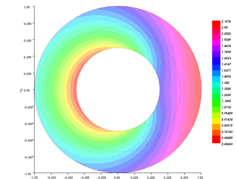
The physical domain $\Omega$ is taken as a 2D annular structure. The accessible boundary $\Gamma_{c}$ is the outer circle, with a ray $R_{c}=1$ and the inaccessible boundary $\Gamma_{i}$ is the inner circle with a ray $R_{i}=0.5$, see Figure 4. The conductivity coefficient is $\lambda=1$, the flux $\Phi=0$ and the heat field $\varphi$ is built from an exact known solution (an academic $u(x,y)=\exp(x)\cos(y)$ used for validation issues).

We use FreemFem++ Hecht et al. (2010) to develop our finite element (FE) solvers. The FE computations are performed with a $P1$-triangular mesh yielding $1,088$ degrees of freedom, the outer and inner boundaries being discretized each with $60$ finite element nodes. From now on, we use the same notations as above for functions to refer to their finite element approximations (values at FE nodes).

As in Section 4.2, to reduce the dimensionality of the problem, the $\eta$ and $\zeta$ being originally vectors of size 60 (the number of nodes at the inner boundary), we interpolate the underlying functions with -natural- splines with $\kappa=8$ coefficients for each quantity, resulting with a decision space of size $d=16$ (instead of the original 120). Each coefficient is bounded between -3 and 3, allowing a large variety of spline shapes.

Since the Neumann condition involving $\Phi$ is known to be the most sensitive to noise, we perturb only this term with an additive noise:

with $\epsilon(\xi)$ a white noise uniformly distributed between $-0.25$ and $0.25$, thus resulting in a randomized vector of dimension 60 (the number of FE nodes on the outer boundary). The resulting variability on $J_{1}(\eta,\zeta,\Phi^{\epsilon})$ and $J_{2}(\eta,\zeta,\Phi^{\epsilon})$ strongly depends on the value of $(\eta,\zeta)$ and can be very large (with coefficients of variation, $y_{i}/\tau_{i}$, from 5% to over 100%).

The original continuous space of the spline coefficients is discretized by generating first two $1000\times 8$ LHD and taking all the combinations between the two designs, ending with space of size $N=10^{6}$ potential strategies. The Bayesian optimization strategy is run with $n_{0}=50$ initial points (chosen by space-filling design) and 150 infill points. Since the noise is very heteroskedastic, we use five repetitions for each trial pair $(\eta,\zeta)$ in order to obtain a rough estimate of the noise variance $\tau_{i}$, and we take the mean over those five repetitions as our observations ($f_{i}$’s). This results with a total budget of $(50+150)\times 5=1,000$ model runs. Let us notice that computing a deterministic NE with fixed-point methods requires about five times this budget on this problem. We followed Algorithm 1 with the SUR criterion, $K=M=20$, selecting $\text{Card}(\mathbb{X}_{\text{sim}})=N_{\text{sim}}=1,296$ simulation points and $\text{Card}(\mathbb{X}_{\text{cand}})=N_{\text{cand}}=256$ candidates.

The algorithm is run five times with different initial points to assess its robustness. The results on the test problem are presented in Figure 5. In the absence of reference (ground truth to be compared to), we show the evolution of the two objectives functions during optimization. All five runs identify very quickly (after 20 iterations, which corresponds to 350 FE evaluations) a similar estimation of the equilibrium, close to the equilibrium of the noiseless problem (which is actually known to be $(0,0)$, Habbal & Kallel (2013)). However, it fails at converging finely to a single, stable value, in particular for $y_{2}$. This is not surprising and can largely be attributed to the difficulty of the problem (with respect to the noise level and dimensionality). Hybrid approaches (using fixed-point strategies for a final local convergence) or sophisticated sampling strategies (increasing the number of repeated simulations gradually with the iterations) may be used to solve this issue (although at the price of a considerably higher computational budget).

References

- Adams & Fournier (2003) Adams, R. A. & Fournier, J. J. (2003). Sobolev spaces, vol. 140. Academic press.
- Álvarez et al. (2011) Álvarez, M. A., Rosasco, L. & Lawrence, N. D. (2011). Kernels for vector-valued functions: A review. Foundations and Trends in Machine Learning 4, 195–266.
- Azzalini & Genz (2016) Azzalini, A. & Genz, A. (2016). The R package mnormt: The multivariate normal and distributions (version 1.5-4).
- Başar (1987) Başar, T. (1987). Relaxation techniques and asynchronous algorithms for on-line computation of noncooperative equilibria. J. Econom. Dynam. Control 11, 531–549.
- Bect et al. (2016) Bect, J., Bachoc, F. & Ginsbourger, D. (2016). A supermartingale approach to gaussian process based sequential design of experiments. arXiv preprint arXiv:1608.01118 .
- Bect et al. (2012) Bect, J., Ginsbourger, D., Li, L., Picheny, V. & Vazquez, E. (2012). Sequential design of computer experiments for the estimation of a probability of failure. Statistics and Computing 22, 773–793.
- Brown et al. (2015) Brown, N., Ganzfried, S. & Sandholm, T. (2015). Hierarchical abstraction, distributed equilibrium computation, and post-processing, with application to a champion no-limit Texas hold’em agent. In Proceedings of the 2015 International Conference on Autonomous Agents and Multiagent Systems.
- Chevalier et al. (2015) Chevalier, C., Emery, X. & Ginsbourger, D. (2015). Fast update of conditional simulation ensembles. Mathematical Geosciences 47, 771–789.
- Chevalier & Ginsbourger (2013) Chevalier, C. & Ginsbourger, D. (2013). Fast computation of the multi-points expected improvement with applications in batch selection. In Learning and Intelligent Optimization. Springer, pp. 59–69.
- Cressie (1993) Cressie, N. (1993). Statistics for spatial data: Wiley series in probability and statistics .
- Dorsch et al. (2013) Dorsch, D., Jongen, H. T. & Shikhman, V. (2013). On structure and computation of generalized nash equilibria. SIAM Journal on Optimization 23, 452–474.
- Facchinei & Kanzow (2010) Facchinei, F. & Kanzow, C. (2010). Generalized nash equilibrium problems. Annals of Operations Research 175, 177–211.
- Fleuret & Geman (1999) Fleuret, F. & Geman, D. (1999). Graded learning for object detection. In Proceedings of the workshop on Statistical and Computational Theories of Vision of the IEEE international conference on Computer Vision and Pattern Recognition (CVPR/SCTV), vol. 2.
- Friedman (1972) Friedman, A. (1972). Stochastic differential games. Journal of differential equations 11, 79–108.
- Games (2016) Games, I.-L. S. C. (2016). Lenient learning in independent-learner stochastic cooperative games. Journal of Machine Learning Research 17, 1–42.
- Garivier et al. (2016) Garivier, A., Kaufmann, E. & Koolen, W. M. (2016). Maximin action identification: A new bandit framework for games. In 29th Annual Conference on Learning Theory.
- Genz & Bretz (2009) Genz, A. & Bretz, F. (2009). Computation of Multivariate Normal and t Probabilities. Lecture Notes in Statistics. Heidelberg: Springer-Verlag.
- Genz et al. (2016) Genz, A., Bretz, F., Miwa, T., Mi, X., Leisch, F., Scheipl, F. & Hothorn, T. (2016). mvtnorm: Multivariate Normal and t Distributions. R package version 1.0-5.
- Gibbons (1992) Gibbons, R. (1992). Game Theory for Applied Economists. Princeton, NJ: Princeton University Press.
- Ginsbourger & Le Riche (2010) Ginsbourger, D. & Le Riche, R. (2010). Towards Gaussian process-based optimization with finite time horizon. In mODa 9–Advances in Model-Oriented Design and Analysis. Springer, pp. 89–96.
- Gonzalez et al. (2016) Gonzalez, J., Osborne, M. & Lawrence, N. (2016). Glasses: Relieving the myopia of Bayesian optimisation. In Proceedings of the 19th International Conference on Artificial Intelligence and Statistics.
- Gramacy & Apley (2015) Gramacy, R. B. & Apley, D. W. (2015). Local gaussian process approximation for large computer experiments. Journal of Computational and Graphical Statistics 24, 561–578.
- Gramacy & Ludkovski (2015) Gramacy, R. B. & Ludkovski, M. (2015). Sequential design for optimal stopping problems. SIAM Journal on Financial Mathematics 6, 748–775.
- Habbal & Kallel (2013) Habbal, A. & Kallel, M. (2013). Neumann-Dirichlet Nash strategies for the solution of elliptic Cauchy problems. SIAM J. Control Optim. 51, 4066–4083.
- Habbal et al. (2004) Habbal, A., Petersson, J. & Thellner, M. (2004). Multidisciplinary topology optimization solved as a Nash game. Int. J. Numer. Meth. Engng 61, 949–963.
- Harsanyi (1973) Harsanyi, J. C. (1973). Games with randomly disturbed payoffs: A new rationale for mixed-strategy equilibrium points. International Journal of Game Theory 2, 1–23.
- Heaton et al. (2017) Heaton, M. J., Datta, A., Finley, A., Furrer, R., Guhaniyogi, R., Gerber, F., Gramacy, R. B., Hammerling, D., Katzfuss, M., Lindgren, F. et al. (2017). Methods for analyzing large spatial data: A review and comparison. arXiv preprint arXiv:1710.05013 .
- Hecht et al. (2010) Hecht, F., Pironneau, O., Le Hyaric, A. & Ohtsuka, K. (2010). Freefem++ v. 2.11. User?s Manual. University of Paris 6.
- Hennig & Schuler (2012) Hennig, P. & Schuler, C. J. (2012). Entropy search for information-efficient global optimization. The Journal of Machine Learning Research 13, 1809–1837.
- Hernández-Lobato et al. (2016) Hernández-Lobato, J. M., Gelbart, M. A., Adams, R. P., Hoffman, M. W. & Ghahramani, Z. (2016). A general framework for constrained bayesian optimization using information-based search. Journal of Machine Learning Research 17, 1–53.
- Hernández-Lobato et al. (2014) Hernández-Lobato, J. M., Hoffman, M. W. & Ghahramani, Z. (2014). Predictive entropy search for efficient global optimization of black-box functions. In Advances in neural information processing systems.
- Hu & Wellman (2003) Hu, J. & Wellman, M. P. (2003). Nash q-learning for general-sum stochastic games. Journal of Machine learning research 4, 1039–1069.
- Isaacs (1965) Isaacs, R. (1965). Differential games. A mathematical theory with applications to warfare and pursuit, control and optimization. John Wiley & Sons, Inc., New York-London-Sydney.
- Jala et al. (2016) Jala, M., Lévy-Leduc, C., Moulines, É., Conil, E. & Wiart, J. (2016). Sequential design of computer experiments for the assessment of fetus exposure to electromagnetic fields. Technometrics 58, 30–42.
- Johanson & Bowling (2009) Johanson, M. & Bowling, M. H. (2009). Data biased robust counter strategies. In Proceedings of the Twelfth International Conference on Artificial Intelligence and Statistics (AISTATS).
- Jones et al. (1998) Jones, D. R., Schonlau, M. & Welch, W. J. (1998). Efficient global optimization of expensive black-box functions. Journal of Global optimization 13, 455–492.
- Kanzow & Steck (2016) Kanzow, C. & Steck, D. (2016). Augmented lagrangian methods for the solution of generalized nash equilibrium problems. SIAM Journal on Optimization 26, 2034–2058.
- Lanctot et al. (2012) Lanctot, M., Burch, N., Zinkevich, M., Bowling, M. & Gibson, R. G. (2012). No-regret learning in extensive-form games with imperfect recall. In Proceedings of the 29th International Conference on Machine Learning (ICML-12).
- León et al. (2014) León, E. R., Pape, A. L., Désidéri, J.-A., Alfano, D. & Costes, M. (2014). Concurrent aerodynamic optimization of rotor blades using a nash game method. Journal of the American Helicopter Society .
- Li & Başar (1987) Li, S. & Başar, T. (1987). Distributed algorithms for the computation of noncooperative equilibria. Automatica J. IFAC 23, 523–533.
- Littman & Stone (2005) Littman, M. L. & Stone, P. (2005). A polynomial-time nash equilibrium algorithm for repeated games. Decision Support Systems 39, 55–66.
- McKay et al. (1979) McKay, M. D., Beckman, R. J. & Conover, W. J. (1979). Comparison of three methods for selecting values of input variables in the analysis of output from a computer code. Technometrics 21, 239–245.
- Mockus (1989) Mockus, J. (1989). Bayesian Approach to Global Optimization: Theory and Applications. Springer.
- Neyman & Sorin (2003) Neyman, A. & Sorin, S. (2003). Stochastic games and applications, vol. 570. Springer Science & Business Media.
- Nishimura et al. (2009) Nishimura, R., Hayashi, S. & Fukushima, M. (2009). Robust nash equilibria in n-person non-cooperative games: Uniqueness and reformulation. Pacific Journal of Optimization 5, 237–259.
- Parr (2012) Parr, J. M. (2012). Improvement Criteria for Constraint Handling and Multiobjective Optimization. Ph.D. thesis, University of Southampton.
- Picheny (2014) Picheny, V. (2014). A stepwise uncertainty reduction approach to constrained global optimization. In Proceedings of the 17th International Conference on Artificial Intelligence and Statistics, vol. 33. JMLR W&CP.
- Picheny & Binois (2017) Picheny, V. & Binois, M. (2017). GPGame: Solving Complex Game problems using Gaussian processes. R package version 0.1.3.
- Plumlee (2014) Plumlee, M. (2014). Fast prediction of deterministic functions using sparse grid experimental designs. Journal of the American Statistical Association 109, 1581–1591.
- R Core Team (2016) R Core Team (2016). R: A Language and Environment for Statistical Computing. R Foundation for Statistical Computing, Vienna, Austria.
- Rasmussen & Williams (2006) Rasmussen, C. E. & Williams, C. (2006). Gaussian Processes for Machine Learning. MIT Press.
- Rosenmüller (1971) Rosenmüller, J. (1971). On a generalization of the lemke–howson algorithm to noncooperative n-person games. SIAM Journal on Applied Mathematics 21, 73–79.
- Roustant et al. (2012) Roustant, O., Ginsbourger, D. & Deville, Y. (2012). DiceKriging, DiceOptim: Two R packages for the analysis of computer experiments by kriging-based metamodeling and optimization. Journal of Statistical Software 51, 1–55.
- Rullière et al. (2016) Rullière, D., Durrande, N., Bachoc, F. & Chevalier, C. (2016). Nested kriging predictions for datasets with a large number of observations. Statistics and Computing , 1–19.
- Scilab Enterprises (2012) Scilab Enterprises (2012). Scilab: Free and Open Source software for numerical computation. Scilab Enterprises, Orsay, France.
- Shahriari et al. (2016) Shahriari, B., Swersky, K., Wang, Z., Adams, R. P. & de Freitas, N. (2016). Taking the human out of the loop: A review of bayesian optimization. Proceedings of the IEEE 104, 148–175.
- Shapley (1953) Shapley, L. S. (1953). Stochastic games. Proceedings of the national academy of sciences 39, 1095–1100.
- Srinivas et al. (2012) Srinivas, N., Krause, A., Kakade, S. M. & Seeger, M. (2012). Information-theoretic regret bounds for gaussian process optimization in the bandit setting. Information Theory, IEEE Transactions on 58, 3250–3265.
- Uryas’ev & Rubinstein (1994) Uryas’ev, S. & Rubinstein, R. Y. (1994). On relaxation algorithms in computation of noncooperative equilibria. IEEE Transactions on Automatic Control 39, 1263–1267.
- Villemonteix et al. (2009) Villemonteix, J., Vazquez, E. & Walter, E. (2009). An informational approach to the global optimization of expensive-to-evaluate functions. Journal of Global Optimization 44, 509–534.
- Wagner et al. (2010) Wagner, T., Emmerich, M., Deutz, A. & Ponweiser, W. (2010). On expected-improvement criteria for model-based multi-objective optimization. In International Conference on Parallel Problem Solving from Nature. Springer.
- Wang & Shan (2007) Wang, G. & Shan, S. (2007). Review of metamodeling techniques in support of engineering design optimization. Journal of Mechanical Design 129, 370.
- Wilson & Nickisch (2015) Wilson, A. & Nickisch, H. (2015). Kernel interpolation for scalable structured gaussian processes (kiss-gp). In International Conference on Machine Learning.
- Žilinskas & Zhigljavsky (2016) Žilinskas, A. & Zhigljavsky, A. (2016). Stochastic global optimization: a review on the occasion of 25 years of informatica. Informatica 27, 229–256.