Synchronization of linear systems via relative actuation

Theory on synchronization in networks of linear systems with general dynamics has reached a certain maturity over the last decade; see, for instance, [7, 9, 6, 13, 1]. A significant part of this theory is founded on the following setup. The nominal individual agent dynamics reads ${\dot{x}}_{i}=Ax_{i}+Bu_{i}$ with $y_{i}=Cx_{i}$. And, the signals available for decision are of the form $z_{i}=\sum_{j}a_{ij}(y_{i}-y_{j})$, where the nonnegative scalars $a_{ij}$ describe the so-called communication topology. Within the boundary of this setup different approaches have yielded various interesting solutions to the synchronization problem, where the universal goal is to drive the agents’ states $x_{i}(t)$ to a common trajectory. E.g., communication delays are considered in [15], $\mathcal{L}_{2}$-gain output-feedback is employed in [2], distributed containment problem is studied in [4]. Among many other works contributing to our wealth of knowledge are [5] on adaptive protocols, [8] on switching topologies, and [14] on optimal state feedback and observer design.

Despite their differences the above-mentioned works allow each agent to have its own independent input $u_{i}$. In this paper we shed this independence. Instead of each agent having its own input we look at the case where each input ($u_{ij}$) is shared by a pair of agents ($i$th and $j$th systems) in the sense displayed in Fig. 1. In particular, we consider the agent dynamics ${x}_{i}^{+}=Ax_{i}+\sum_{j}B_{ij}u_{ij}$ with $y_{ij}=C_{ij}(x_{i}-x_{j})$, where (i) the actuation is relative (i.e., $B_{ij}u_{ij}+B_{ji}u_{ji}=0$) and (ii) the signals available for decision read $z_{i}=\sum_{j}C_{ij}^{T}y_{ij}$. In our setup the input matrices $B_{ij}$ are allowed to be incommensurable in the sense that there need not exist a common $B$ satisfying $B_{ij}=a_{ij}B$ with scalar $a_{ij}$. In fact, two input matrices do not even have to be of the same size. The same goes for the output matrices $C_{ij}$. The problem we study here is that of decentralized stabilization (of the synchronization subspace) by choosing appropriate inputs $u_{ij}$ based on the relative measurements $y_{ij}$. As a solution to this problem we construct a distributed algorithm that achieves synchronization via dynamic relative output feedback.

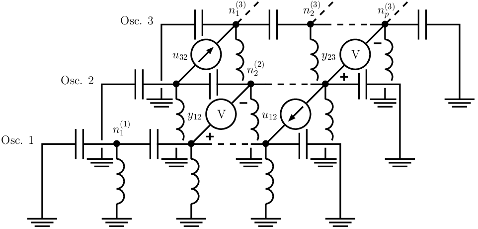
Let us now illustrate our setup on an example network. Consider the array of identical electrical oscillators shown in Fig. 2, where each oscillator (of order $2p$) has $p$ nodes (excepting the ground node) and the $k$th node of the $i$th oscillator is denoted by $n_{k}^{(i)}$. The actuation is achieved through current sources while the measurements are collected through voltmeters. Each current source/voltmeter connects a pair of nodes (belonging to two separate oscillators) with the same index number, say $n_{k}^{(i)}$ and $n_{k}^{(j)}$. It is not difficult to see that this architecture enjoys the form ${\dot{x}}_{i}=Ax_{i}+\sum_{j}B_{ij}u_{ij}$ with $y_{ij}=C_{ij}(x_{i}-x_{j})$ and, since each current source connects two nodes with the same index number, the actuation throughout the network is relative. Furthermore, the input matrices $B_{ij}$ are incommensurable. For instance, while the current source $u_{32}$ connects $n_{1}^{(3)}$ and $n_{1}^{(2)}$, the current source $u_{12}$ connects $n_{p}^{(1)}$ and $n_{p}^{(2)}$. Since for these two current sources the indices (1 and $p$) of the nodes they are associated to are different, we cannot find a scalar $a$ that satisfies $B_{12}=aB_{32}$. Likewise, the output matrices $C_{ij}$ too are incommensurable.

We begin the remainder of the paper by providing the formal description of the array we study. After that we present a distributed algorithm that generates control inputs through dynamic output feedback, followed by our main (and only) theorem, which states that this algorithm with suitable parameter choice achieves synchronization. To prove the theorem we first obtain the explicit expression of the closed-loop system the array becomes under the algorithm. Once the righthand side of the closed loop is computed we proceed to establish stability and thus complete the proof of the main result.

Consider an array of $q$ discrete-time linear time-invariant systems

$$x_{i}^{+}&=Ax_{i}+\sum_{j=1}^{q}B_{ij}u_{ij}\\ y_{ij}=C_{ij}(x_{i}-x_{j})\,;\qquad i,\,j=1,\,2,\,\ldots,\,q$$

(1)

where $x_{i}\in{\mathbb{R}}^{n}$ is the state of the $i$th system with $A\in{\mathbb{R}}^{n\times n}$, $x_{i}^{+}$ denotes the state at the next time instant, $u_{ij}=u_{ji}\in{\mathbb{R}}^{p_{ij}}$ is the $ij$th input with $B_{ij}=-B_{ji}\in{\mathbb{R}}^{n\times p_{ij}}$, and $y_{ij}=y_{ji}\in{\mathbb{R}}^{m_{ij}}$ is the $ij$th (relative) output with $C_{ij}=-C_{ji}\in{\mathbb{R}}^{m_{ij}\times n}$. We interpret the equality $u_{ij}=u_{ji}$ as that $u_{ij}$ and $u_{ji}$ are different notations for the same single variable. Same goes for the oneness of $y_{ij}$ and $y_{ji}$. Note that we have to have $B_{ii}=0$ and $C_{ii}=0$. Note also that the actuation is relative because $B_{ij}u_{ij}+B_{ji}u_{ji}=0$. Hence the average of the states $x_{\rm av}=q^{-1}\sum x_{i}$ evolves independently of the inputs driving the array, i.e., we have $x_{\rm av}^{+}=Ax_{\rm av}$. The ordered collections $(B_{ij})_{i,j=1}^{q}$ and $(C_{ij})_{i,j=1}^{q}$ are denoted by $(B_{::})$ and $(C_{::})$, respectively. The value of the solution of the $i$th system at the $k$th time instant ($k=0,\,1,\,\ldots$) is denoted by $x_{i}[k]$. The meanings of $u_{ij}[k]$ and $y_{ij}[k]$ should be clear.

The array (1) gives rise to the following single big system

$${\mathbf{x}}^{+}&={\mathbf{A}}{\mathbf{x}}+{\mathbf{B}}{\mathbf{u}}\\ {\mathbf{y}}={\mathbf{C}}{\mathbf{x}}$$

(2)

where ${\mathbf{x}}=[x_{1}^{T}\ x_{2}^{T}\ \cdots\ x_{q}^{T}]^{T}$ is the state, ${\mathbf{u}}=[u_{12}^{T}\ u_{13}^{T}\ \cdots\ u_{1q}^{T}\,|\,u_{23}^{T}\ u_{24}^{T}\ \cdots\ u_{2q}^{T}\,|\,\cdots\,|\,u_{(q-1)q}^{T}]^{T}$ is the input, and ${\mathbf{y}}=[y_{12}^{T}\ y_{13}^{T}\ \cdots\ y_{1q}^{T}\,|\,y_{23}^{T}\ y_{24}^{T}\ \cdots\ y_{2q}^{T}\,|\,\cdots\,|\,y_{(q-1)q}^{T}]^{T}$ is the output. Clearly, we have

$\displaystyle{\mathbf{A}}=[I_{q}\otimes A]$

where $I_{q}\in{\mathbb{R}}^{q\times q}$ is the identity matrix (which we may also denote by $I$ when its dimension is either clear from the context or immaterial),

$\displaystyle{\mathbf{B}}={\rm inc}\,(B_{::}):=\left[\begin{array}[]{cccc|cccc|c|c}B_{12}&B_{13}&\cdots&B_{1q}&0&0&\cdots&0&\cdots&0\\ -B_{12}&0&\cdots&0&B_{23}&B_{24}&\cdots&B_{2q}&\cdots&0\\ 0&-B_{13}&\cdots&0&-B_{23}&0&\cdots&0&\cdots&0\\ 0&0&\cdots&0&0&-B_{24}&\cdots&0&\cdots&0\\ \vdots&\vdots&\ddots&\vdots&\vdots&\vdots&\ddots&\vdots&\ddots&\vdots\\ 0&0&\cdots&0&0&0&\cdots&0&\cdots&B_{(q-1)q}\\ 0&0&\cdots&-B_{1q}&0&0&\cdots&-B_{2q}&\cdots&-B_{(q-1)q}\end{array}\right]$

and

$\displaystyle{\mathbf{C}}=[{\rm inc}\,(C_{::}^{T})]^{T}\,.$

The notational choice “inc” has to do with that the structure of ${\mathbf{B}}$ resembles that of the incidence matrix of a graph. Let $\mathcal{S}_{n}={\rm range}\,[{\mathbf{1}}_{q}\otimes I_{n}]$, where ${\mathbf{1}}_{q}\in{\mathbb{R}}^{q}$ is the vector of all ones. The set $\mathcal{S}_{n}\subset({\mathbb{R}}^{n})^{q}$ is called the synchronization subspace, whose orthogonal complement, the disagreement subspace, is denoted by $\mathcal{S}_{n}^{\perp}$. Let us construct the matrices one is all too familiar with

$\displaystyle{\mathbf{W}}_{\rm c}=[{\mathbf{B}}\ {\mathbf{A}}{\mathbf{B}}\ \cdots\ {\mathbf{A}}^{n-1}{\mathbf{B}}]\,,\quad{\mathbf{W}}_{\rm o}=\left[\begin{array}[]{c}{\mathbf{C}}\\ {\mathbf{C}}{\mathbf{A}}\\ \vdots\\ {\mathbf{C}}{\mathbf{A}}^{n-1}\end{array}\right]\,.$

We have ${\rm range}\,{\mathbf{W}}_{\rm c}\subset\mathcal{S}_{n}^{\perp}$ and ${\rm null}\,{\mathbf{W}}_{\rm c}\supset\mathcal{S}_{n}$ by construction. Now we define (relative) controllability and (relative) observability concerning the array (1).

Note that $[A,\,(B_{::})]$ is controllable if and only if $[(B_{::}^{T}),\,A^{T}]$ is observable. Necessary and sufficient conditions for controllability and observability (in the above sense) are reported in [12] and [11], respectively. Henceforth we assume:

The array (1) is both controllable and observable.

In the next section we present a distributed synchronization algorithm that generates input signals $u_{ij}$ for the array (1) based on the measurements $y_{ij}$. This algorithm is meant to achieve convergence $\|x_{i}[k]-x_{j}[k]\|\to 0$ for all pairs $(i,\,j)$ and all initial conditions.

There are four design parameters to be chosen for the algorithm: the integers $N_{\rm c},\,N_{\rm o}\geq n$ and the real numbers $\tau_{\rm c},\,\tau_{\rm o}>0$. The variables employed are denoted by $\lambda_{i},\,{\hat{x}}_{i},\,\xi_{i}\in{\mathbb{R}}^{n}$, and $w_{ij}\in({\mathbb{R}}^{p_{ij}})^{N_{\rm c}}$ for $i,\,j=1,\,2,\,\ldots,\,q$. The variables ${\hat{x}}_{i}$ are purely discrete and their values at the $k$th discrete time instant is denoted by ${\hat{x}}_{i}[k]$. The remaining variables, at each $k$, solve certain differential equations, the solutions of which are denoted by $\lambda_{i}[k,\,t),\,\xi_{i}[k,\,t)$, and $w_{ij}[k,\,t)$ with $t\in{\mathbb{R}}$ being the continuous time variable. Now, the algorithm generating the control inputs $u_{ij}[k]$ for the array (1) is as follows.

$${\dot{w}}_{ij}[k,\,t)&=-w_{ij}[k,\,t)-[B_{ij}\ AB_{ij}\ \cdots\ A^{N_{\rm c}-1}B_{ij}]^{T}(\lambda_{i}[k,\,t)-\lambda_{j}[k,\,t)){}\\ {\dot{\lambda}}_{i}[k,\,t)=A^{N_{\rm c}}{\hat{x}}_{i}[k]+\sum_{j=1}^{q}\,[B_{ij}\ AB_{ij}\ \cdots\ A^{N_{\rm c}-1}B_{ij}]w_{ij}[k,\,t){}\\ {\hat{x}}_{i}[k+1]=A{\hat{x}}_{i}[k]+A^{N_{\rm o}}\xi_{i}[k,\,\tau_{\rm o})+\sum_{j=1}^{q}B_{ij}u_{ij}[k]{}\\ {\dot{\xi}}_{i}[k,\,t)=-\sum_{\ell=0}^{N_{\rm o}-1}\sum_{j=1}^{q}A^{\ell T}C_{ij}^{T}C_{ij}A^{\ell}(\xi_{i}[k,\,t)-\xi_{j}[k,\,t))\\ \qquad+\sum_{j=1}^{q}A^{(N_{\rm o}-1)T}C_{ij}^{T}(y_{ij}[k]-C_{ij}({\hat{x}}_{i}[k]-{\hat{x}}_{j}[k])){}\\ u_{ij}[k]=[\,\underbrace{[0\ \cdots\ 0\ 1]}_{\displaystyle N_{\rm c}\,\mbox{terms}}\otimes I_{p_{ij}}]w_{ij}[k,\,\tau_{\rm c}){}$$

(5)

where, for all $k$, the initial conditions for integrations are set as

$\displaystyle\lambda_{i}[k,\,0)=0\,,\quad\xi_{i}[k,\,0)=0\,,\quad w_{ij}[k,\,0)=0\,.$

As for ${\hat{x}}_{i}$, the initial conditions ${\hat{x}}_{i}[0]$ can be chosen arbitrarily. Having described our algorithm, we can now state what it does. Below is our main result.

In the remainder of the paper we construct the proof of Theorem 1. To this end, we first obtain the discrete-time closed-loop dynamics explicitly. Then we study its stability.

In this section we compute the closed-loop dynamics governing the system (2) under the algorithm (5). Namely, we obtain explicit expressions for the matrices ${\mathbf{K}}$ and ${\mathbf{L}}$ which should appear as

$${\mathbf{x}}^{+}&={\mathbf{A}}{\mathbf{x}}-{\mathbf{B}}{\mathbf{K}}\hat{}{\mathbf{x}}{}\\ \hat{}{\mathbf{x}}^{+}={\mathbf{A}}\hat{}{\mathbf{x}}-{\mathbf{B}}{\mathbf{K}}\hat{}{\mathbf{x}}+{\mathbf{L}}({\mathbf{y}}-{\mathbf{C}}\hat{}{\mathbf{x}}){}$$

(6)

where $\hat{}{\mathbf{x}}=[\hat{x}_{1}^{T}\ \hat{x}_{2}^{T}\ \cdots\ \hat{x}_{q}^{T}]^{T}$ and $\hat{x}_{i}$ are updated via (). We begin with ${\mathbf{K}}$.

In the previous section we obtained the explicit expression for the righthand side of (6) by computing the gains ${\mathbf{K}}$ and ${\mathbf{L}}$. Now we study the behavior of the closed-loop system. Our goal is to show that (under appropriate choices of the parameters $\tau_{\rm c},\tau_{\rm o}$) for all initial conditions ${\mathbf{x}}[0]$ and $\hat{}{\mathbf{x}}[0]$ the solution ${\mathbf{x}}[k]$ enjoys the convergence $\|{\mathbf{x}}[k]\|_{\mathcal{S}_{n}}\to 0$, where $\|\cdot\|_{\mathcal{S}_{n}}$ denotes the Euclidean distance to the subspace $\mathcal{S}_{n}$. By proving this convergence we will have established Theorem 1. For our analysis we borrow the following result due to Kleinman [3].¹¹ 1 Kleinman assumes that the matrix $F$ is invertible. This assumption however is superfluous; see [10].

Define the reduced state ${\mathbf{x}}_{\rm r}={\mathbf{D}}^{T}{\mathbf{x}}$ and the error ${\mathbf{e}}_{\rm r}={\mathbf{D}}^{T}(\hat{}{\mathbf{x}}-{\mathbf{x}})$. Note that $\|{\mathbf{x}}_{\rm r}\|=\|{\mathbf{x}}\|_{\mathcal{S}_{n}}$. Also, define the following reduced parameters

$\displaystyle{\mathbf{A}}_{\rm r}={\mathbf{D}}^{T}{\mathbf{A}}{\mathbf{D}}\,,\quad{\mathbf{B}}_{\rm r}={\mathbf{D}}^{T}{\mathbf{B}}\,,\quad{\mathbf{C}}_{\rm r}={\mathbf{C}}{\mathbf{D}}\,,\quad{\mathbf{K}}_{\rm r}={\mathbf{K}}{\mathbf{D}}\,,\quad{\mathbf{L}}_{\rm r}={\mathbf{D}}^{T}{\mathbf{L}}\,.$

Note that Lemma 5 and Lemma 11 imply ${\mathbf{K}}={\mathbf{K}}{\mathbf{D}}{\mathbf{D}}^{T}$. Using the structural properties of our matrices ${\mathbf{A}},\,{\mathbf{B}},\,{\mathbf{C}}$ emphasized in Lemmas 1, 8, and 11, we now proceed to obtain the dynamics for ${\mathbf{x}}_{\rm r}$ and ${\mathbf{e}}_{\rm r}$. Consider (). We can write

	$\displaystyle{\mathbf{x}}_{\rm r}^{+}$	$\displaystyle=$	$\displaystyle{\mathbf{D}}^{T}{\mathbf{x}}^{+}$
		$\displaystyle=$	$\displaystyle{\mathbf{D}}^{T}{\mathbf{A}}{\mathbf{x}}-{\mathbf{D}}^{T}{\mathbf{B}}{\mathbf{K}}\hat{}{\mathbf{x}}$
		$\displaystyle=$	$\displaystyle{\mathbf{D}}^{T}{\mathbf{A}}{\mathbf{D}}{\mathbf{D}}^{T}{\mathbf{x}}-{\mathbf{D}}^{T}{\mathbf{B}}{\mathbf{K}}{\mathbf{D}}{\mathbf{D}}^{T}\hat{}{\mathbf{x}}$
		$\displaystyle=$	$\displaystyle{\mathbf{A}}_{\rm r}{\mathbf{x}}_{\rm r}-{\mathbf{B}}_{\rm r}{\mathbf{K}}_{\rm r}({\mathbf{x}}_{\rm r}+{\mathbf{e}}_{\rm r})$
		$\displaystyle=$	$\displaystyle[{\mathbf{A}}_{\rm r}-{\mathbf{B}}_{\rm r}{\mathbf{K}}_{\rm r}]{\mathbf{x}}_{\rm r}-{\mathbf{B}}_{\rm r}{\mathbf{K}}_{\rm r}{\mathbf{e}}_{\rm r}\,.$

As for ${\mathbf{e}}_{\rm r}$, the dynamics (6) yields

	$\displaystyle{\mathbf{e}}_{\rm r}^{+}$	$\displaystyle=$	$\displaystyle{\mathbf{D}}^{T}(\hat{}{\mathbf{x}}^{+}-{\mathbf{x}}^{+})$
		$\displaystyle=$	$\displaystyle{\mathbf{D}}^{T}({\mathbf{A}}\hat{}{\mathbf{x}}+{\mathbf{L}}({\mathbf{C}}{\mathbf{x}}-{\mathbf{C}}\hat{}{\mathbf{x}})-{\mathbf{A}}{\mathbf{x}})$
		$\displaystyle=$	$\displaystyle[{\mathbf{D}}^{T}{\mathbf{A}}-{\mathbf{D}}^{T}{\mathbf{L}}{\mathbf{C}}](\hat{}{\mathbf{x}}-{\mathbf{x}})$
		$\displaystyle=$	$\displaystyle[{\mathbf{D}}^{T}{\mathbf{A}}{\mathbf{D}}{\mathbf{D}}^{T}-{\mathbf{D}}^{T}{\mathbf{L}}{\mathbf{C}}{\mathbf{D}}{\mathbf{D}}^{T}](\hat{}{\mathbf{x}}-{\mathbf{x}})$
		$\displaystyle=$	$\displaystyle[{\mathbf{D}}^{T}{\mathbf{A}}{\mathbf{D}}-{\mathbf{D}}^{T}{\mathbf{L}}{\mathbf{C}}{\mathbf{D}}]{\mathbf{D}}^{T}(\hat{}{\mathbf{x}}-{\mathbf{x}})$
		$\displaystyle=$	$\displaystyle[{\mathbf{A}}_{\rm r}-{\mathbf{L}}_{\rm r}{\mathbf{C}}_{\rm r}]{\mathbf{e}}_{\rm r}\,.$

Hence the overall dynamics for the pair $({\mathbf{x}}_{\rm r},\,{\mathbf{e}}_{\rm r})$ reads

$\displaystyle\left[\begin{array}[]{c}{\mathbf{x}}_{\rm r}\\ {\mathbf{e}}_{\rm r}\end{array}\right]^{+}=\underbrace{\left[\begin{array}[]{cc}{\mathbf{A}}_{\rm r}-{\mathbf{B}}_{\rm r}{\mathbf{K}}_{\rm r}&-{\mathbf{B}}_{\rm r}{\mathbf{K}}_{\rm r}\\ 0&{\mathbf{A}}_{\rm r}-{\mathbf{L}}_{\rm r}{\mathbf{C}}_{\rm r}\end{array}\right]}_{\displaystyle{\mathbf{\Phi}}_{\rm r}}\left[\begin{array}[]{c}{\mathbf{x}}_{\rm r}\\ {\mathbf{e}}_{\rm r}\end{array}\right]\,.$

Next, we show that the block diagonal entries in (5) can be made Schur by choosing $\tau_{\rm c}$ and $\tau_{\rm o}$ large enough. To this end, let us define the following $(q-1)n\times(q-1)n$ matrices.

	$\displaystyle\theta_{\rm c}(\tau)$	$\displaystyle=$	$\displaystyle{\mathbf{D}}^{T}{\mathbf{B}}\left[{\mathbf{B}}^{T}{\mathbf{A}}^{(N_{\rm c}-1)T}{\mathbf{D}}[{\mathbf{D}}^{T}{\mathbf{R}}{\mathbf{R}}^{T}{\mathbf{D}}]^{-1}{\mathbf{D}}^{T}{\mathbf{R}}-[e_{N_{\rm c}}^{T}\otimes I]\ \ \ {\mathbf{B}}^{T}{\mathbf{A}}^{(N_{\rm c}-1)T}{\mathbf{D}}[{\mathbf{D}}^{T}{\mathbf{R}}{\mathbf{R}}^{T}{\mathbf{D}}]^{-1}\right]$
			$\displaystyle\qquad\times[e^{\Lambda\tau}]\times\left[\begin{array}[]{c}0\\ {\mathbf{D}}^{T}{\mathbf{A}}^{N_{\rm c}}\end{array}\right]{\mathbf{D}}$
	$\displaystyle\theta_{\rm o}(\tau)$	$\displaystyle=$	$\displaystyle{\mathbf{D}}^{T}{\mathbf{A}}^{N_{\rm o}}{\mathbf{D}}\Gamma^{-1}[e^{-\Gamma\tau}]{\mathbf{D}}^{T}{\mathbf{A}}^{(N_{\rm o}-1)T}{\mathbf{C}}^{T}{\mathbf{C}}{\mathbf{D}}\,.$

Now we can write by Lemmas 1, 5, and 11

	$\displaystyle{\mathbf{A}}_{\rm r}-{\mathbf{B}}_{\rm r}{\mathbf{K}}_{\rm r}$	$\displaystyle=$	$\displaystyle{\mathbf{A}}_{\rm r}-{\mathbf{D}}^{T}{\mathbf{B}}{\mathbf{K}}{\mathbf{D}}$		(43)
		$\displaystyle=$	$\displaystyle{\mathbf{A}}_{\rm r}-{\mathbf{D}}^{T}{\mathbf{B}}{\mathbf{B}}^{T}{\mathbf{A}}^{(N_{\rm c}-1)T}{\mathbf{D}}[{\mathbf{D}}^{T}{\mathbf{R}}{\mathbf{R}}^{T}{\mathbf{D}}]^{-1}{\mathbf{D}}^{T}{\mathbf{A}}^{N_{\rm c}}{\mathbf{D}}+\theta_{\rm c}(\tau_{\rm c})$
		$\displaystyle=$	$\displaystyle{\mathbf{A}}_{\rm r}-{\mathbf{B}}_{\rm r}{\mathbf{B}}_{\rm r}^{T}{\mathbf{A}}_{\rm r}^{(N_{\rm c}-1)T}[{\mathbf{D}}^{T}{\mathbf{R}}{\mathbf{R}}^{T}{\mathbf{D}}]^{-1}{\mathbf{A}}_{\rm r}^{N_{\rm c}}+\theta_{\rm c}(\tau_{\rm c})$
		$\displaystyle=$	$\displaystyle\underbrace{{\mathbf{A}}_{\rm r}-{\mathbf{B}}_{\rm r}{\mathbf{B}}_{\rm r}^{T}{\mathbf{A}}_{\rm r}^{(N_{\rm c}-1)T}\left(\sum_{\ell=0}^{N_{\rm c}-1}{\mathbf{A}}_{\rm r}^{\ell}{\mathbf{B}}_{\rm r}{\mathbf{B}}_{\rm r}^{T}{\mathbf{A}}_{\rm r}^{\ell T}\right)^{-1}{\mathbf{A}}_{\rm r}^{N_{\rm c}}}_{\displaystyle{\mathbf{H}}_{\rm c}}+\,\theta_{\rm c}(\tau_{\rm c})$

where we used ${\mathbf{D}}^{T}{\mathbf{R}}=[{\mathbf{B}}_{\rm r}\ {\mathbf{A}}_{\rm r}{\mathbf{B}}_{\rm r}\ \cdots\ {\mathbf{A}}_{\rm r}^{N_{\rm c}-1}{\mathbf{B}}_{\rm r}]$ and ${\mathbf{A}}_{\rm r}^{\ell}={\mathbf{D}}^{T}{\mathbf{A}}^{\ell}{\mathbf{D}}$. Similarly, by Lemmas 8, 10, and 11 we obtain

	$\displaystyle{\mathbf{A}}_{\rm r}-{\mathbf{L}}_{\rm r}{\mathbf{C}}_{\rm r}$	$\displaystyle=$	$\displaystyle{\mathbf{A}}_{\rm r}-{\mathbf{D}}^{T}{\mathbf{L}}{\mathbf{C}}{\mathbf{D}}$		(44)
		$\displaystyle=$	$\displaystyle{\mathbf{A}}_{\rm r}-{\mathbf{D}}^{T}{\mathbf{A}}^{N_{\rm o}}{\mathbf{D}}\Gamma^{-1}{\mathbf{D}}^{T}{\mathbf{A}}^{(N_{\rm o}-1)T}{\mathbf{C}}^{T}{\mathbf{C}}{\mathbf{D}}+\theta_{\rm o}(\tau_{\rm o})$
		$\displaystyle=$	$\displaystyle{\mathbf{A}}_{\rm r}-{\mathbf{A}}_{\rm r}^{N_{\rm o}}[{\mathbf{D}}^{T}{\mathbf{Q}}^{T}{\mathbf{Q}}{\mathbf{D}}]^{-1}{\mathbf{A}}_{\rm r}^{(N_{\rm o}-1)T}{\mathbf{C}}_{\rm r}^{T}{\mathbf{C}}_{\rm r}+\theta_{\rm o}(\tau_{\rm o})$
		$\displaystyle=$	$\displaystyle\underbrace{{\mathbf{A}}_{\rm r}-{\mathbf{A}}_{\rm r}^{N_{\rm o}}\left(\sum_{\ell=0}^{N_{\rm o}-1}{\mathbf{A}}_{\rm r}^{\ell T}{\mathbf{C}}_{\rm r}^{T}{\mathbf{C}}_{\rm r}{\mathbf{A}}_{\rm r}^{\ell}\right)^{-1}{\mathbf{A}}_{\rm r}^{(N_{\rm o}-1)T}{\mathbf{C}}_{\rm r}^{T}{\mathbf{C}}_{\rm r}}_{\displaystyle{\mathbf{H}}_{\rm o}}+\,\theta_{\rm o}(\tau_{\rm o})$

where we used ${\mathbf{D}}^{T}{\mathbf{Q}}^{T}=[{\mathbf{C}}_{\rm r}^{T}\ {\mathbf{A}}_{\rm r}^{T}{\mathbf{C}}_{\rm r}^{T}\ \cdots\ {\mathbf{A}}_{\rm r}^{(N_{\rm o}-1)T}{\mathbf{C}}_{\rm r}^{T}]$.

References

• [1] Y. Cao, W. Yu, W. Ren, and G. Chen. An overview of recent progress in the study of distributed multi-agent coordination. IEEE Transactions on Industrial Informatics, 9:427–438, 2013.
• [2] Q. Jiao, H. Modares, F.L. Lewis, S. Xu, and L. Xie. Distributed ℒ2\mathcal{L}_{2}-gain output-feedback control of homogeneous and heterogeneous systems. Automatica, 71:361–368, 2016.
• [3] D.L. Kleinman. Stabilizing a discrete constant linear system with application to iterative methods for solving the Riccati equation. IEEE Transactions on Automatic Control, 19:252–254, 1974.
• [4] Z. Li, W. Ren, X. Liu, and M. Fu. Distributed containment control of multi-agent systems with general linear dynamics in the presence of multiple leaders. International Journal of Robust and Nonlinear Control, 23:534–547, 2013.
• [5] Z. Li, W. Ren, X. Liu, and L. Hie. Distributed consensus of linear multi-agent systems with adaptive dynamic protocols. Automatica, 49:1986–1995, 2013.
• [6] Z.K. Li, Z.S. Duan, G.R. Chen, and L. Huang. Consensus of multiagent systems and synchronization of complex networks: A unified viewpoint. IEEE Transactions on Circuits and Systems I: Regular Papers, 57:213–224, 2010.
• [7] L. Scardovi and R. Sepulchre. Synchronization in networks of identical linear systems. Automatica, 45:2557–2562, 2009.
• [8] J.H. Seo, J. Back, H. Kim, and H. Shim. Output feedback consensus for high-order linear systems having uniform ranks under switching topology. IET Control Theory and Applications, 6:1118–1124, 2012.
• [9] J.H. Seo, H. Shim, and J. Back. Consensus of high-order linear systems using dynamic output feedback compensator: Low gain approach. Automatica, 45:2659–2664, 2009.
• [10] S.E. Tuna. A dual pair of optimization-based formulations for estimation and control. Automatica, 51:18–26, 2015.
• [11] S.E. Tuna. Observability through matrix-weighted graph, 2016. arXiv:1603.07637 [math.DS].
• [12] S.E. Tuna. Positive controllability of networks under relative actuation, 2017. arXiv:1707.05502 [math.DS].
• [13] T. Yang, S. Roy, and A. Saberi. Constructing consensus controllers for networks with identical general linear agents. International Journal of Robust and Nonlinear Control, 21:1237–1256, 2011.
• [14] H. Zhang, F.L. Lewis, and A. Das. Optimal design for synchronization of cooperative systems: State feedback, observer and output feedback. IEEE Transactions on Automatic Control, 56:1948–1952, 2011.
• [15] B. Zhou and Z. Lin. Consensus of high-order multi-agent systems with large input and communication delays. Automatica, 50:452–464, 2014.