Multiscale response of ionic systems to a spatially varying electric field

The response is evaluated for two simple models: (i) one model for molten salt proposed by Hansen and McDonald [1] and (ii) one modified model for ionic liquids used by Chapela et al. [15]. For the molten salt the ions are simple spherical particles with same mass and point charges $\pm q$. The van der Waals interaction is the inverse power law function $V(r)=\epsilon(\sigma/r)^{9}$, where $r$ is the distance between two ions, $\epsilon$ and $\sigma$ define the energy and length scale, respectively. The Coulomb interactions are calculated through the shifted force method [16, 17], $\mathbf{F}(r)=q_{i}q_{j}(1/r^{2}-1/r_{c}^{2})\mathbf{r}/r$, for $r\leq r_{c}$. Here $\mathbf{r}$ is the vector of separation with magnitude $r$, and $r_{c}$ is the cut-off radius set to $r_{c}=3\sigma$; this cut-off distance is also used for the van der Waals interactions. The positions of the particles are integrated forward in time with the leap-frog algorithm [18] and the temperature is controlled using a Nosé-Hoover thermostat [19, 20]. In all simulations the total ion number density is $n=0.368\sigma^{-3}$; the number of ions are 1000, giving 500 ion-pairs. Two different temperatures are simulated, $T=0.0177\epsilon/k_{B}$ and $1.0177\epsilon/k_{B}$, the former being a realistic temperature for the model. To simulate the Debye-Hückel regime $k_{B}T\gg q\phi$ the ion-ion Coulomb interactions are removed whilst keeping the temperature fixed at $T=1.0177\epsilon/k_{B}$; this system is symbolized using $T_{\infty}$. Alternatively, one can perform simulations at very high temperatures, but this will result in numerical instabilities. In the following all quantities are given in units of $\sigma$, $\epsilon$, $q$, and mass $m$, and as it is common practise these the units are not written explicitly.

For the simple molten salt system the shifted force method can be tested against the direct Ewald summation method [21]. From equilibrium simulations it was found from the structure that the Ewald method converges satisfactory using 124 replica systems and that it agrees with the data from the shifted force method, see also Ref. 17. For the non-equilibrium situation at $T=1.0177$ the Ewald and shifted force methods yield same results for all wavevectors tested $0<k<2.2$.

The modified ionic liquid model is composed of cations with a spherical point charge particle (head group) and two spherical non-charged tail particles. The particles in the cation are linearly connected using a simple spring force $\mathbf{F}=-k(r-1)\mathbf{r}/r$, where $k=100$ is the spring constant. Anions are simple spherical point charge particles [15]. Rather than a hard-sphere type potential in the original model, the van der Waals interactions are here given through the Weeks-Chandler-Andersen potential [22] $V(r)=4((1/r)^{12}-(1/r)^{6})$, where the cut-off is set at $r_{c}=2^{1/6}$.The Coulomb interaction is given by the Yukawa potential $V(r)=q^{2}e^{-r/\lambda_{D}}/r$, with $\lambda_{D}=1/2$ corresponding to a relative small Debye screening length and the reduced charge is $q=4$. The cut-off distance for the Yukawa potential is set to $r_{c}=2.5$. The state point is $(n,T)=(1,1)$ and the simulation method is the same as for the molten salt simulations. This choice of parameters gives, qualitatively, the fluid structure observed in different ionic liquid [23, 24]. The number of particles are 864, that is, 216 ion pairs.

Simulations of the non-equilibrium system is also performed. Here an additional force from the external field, Eq. (3), is added to the total force experienced by the ions $\mathbf{F}_{i}^{\mathrm{ext}}=q_{i}E^{\mathrm{ext}}\mathbf{k}$, where $\mathbf{k}$ is the unit vector parallel to the $z$-axis.

The wavevector dependent diffusivity can be obtained as follows. The Gaussian approximation [2, 25] relates the diffusion coefficient to the incoherent intermediate scattering function (or the self-part of the density-density correlations), so in the diffusive regime, i.e., for large $t$, this is here generalized to

The Fourier-Laplace transformation is

which gives an expression for the wavevector dependent diffusivity in the limit of zero frequency

Microscopically the intermediate scattering function is defined from the ensemble average [25]

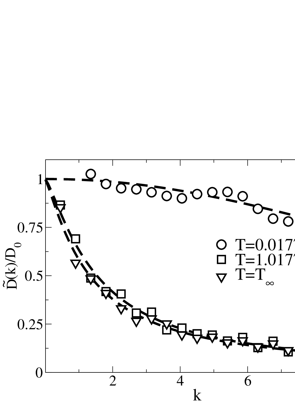
where $N$ is the number of ions and is thus a single particle property. In Fig. 1 (a) the intermediate scattering function is plotted for different wavevectors in the case of $T=0.0177$. Also, shown as punctured lines $f(k,t)=e^{-\frac{1}{6}\langle\Delta r^{2}\rangle k^{2}t}$, where $\langle\Delta r^{2}\rangle$ is the particle mean square displacement. It is seen that the Gaussian approximation holds surprisingly well for this model validating Eq.(19). The data are Fourier-Laplace transformed and the Gaussian diffusion kernel is found from Eq. (21); the results are plotted in Fig. 1 (b). The function

is fitted to data where the zero wavevector diffusion coefficient, $D_{0}$, is found from the mean square displacement $\langle\Delta r^{2}\rangle=2D_{0}t$ for $t\rightarrow\infty$. It is observed that the normalized kernel is identical for the two cases $T=1.0177$ and $T=T_{\infty}$. For $T=0.0177$ the diffusivity features a relative low wavevector dependency in the range studied here and we have $\widetilde{\chi}(k)\propto S_{ZZ}(k)$ according to Eq. (18).

Next the charge-charge structure is evaluated. This is defined as [2]

where $\rho_{q}(\mathbf{k},0)=\sum_{i}q_{i}e^{-i\mathbf{k}\cdot\mathbf{r}_{i}}$. Note, this is a collective property. For non-zero wavevectors $S_{zz}(k)$ can also be calculated from the radial distribution functions, see e.g. Ref. 1,

where $\Delta g(r)$ is the difference between the cation-cation and cation-anion radial distribution functions, $\Delta g(r)=g_{++}(r)-g_{+-}(r)$. The charge-charge structure is plotted in Fig. 2 for the three different systems; symbols are data from Eq. (24) and lines are $S_{zz}$ calculated from Eq. (25). As expected we observe a zero screening, $S_{zz}=1$, for $T=T_{\infty}$, but non-negligible screening for $T=1.0177$ and $T=0.0177$.

From Eq. (16) the Fourier components of $\chi$ can be evaluated, the results is shown in Fig. 3 (a). The evaluation is based on the fit of the diffusion kernel, Eq. (23), and the integral expression for the charge-charge structure, Eq. (25). First, for zero screening, $T=T_{\infty}$, the response function is monotonically decaying with respect to wavevector. This behavior is typically observed for the diffusion and viscosity kernels [8]. For non-zero screening the response features a maximum depending on temperature; the characteristic wave length $l=2\pi/k_{\text{max}}$ where $k_{\text{max}}$ is the wavevector corresponding to maximum in $\widetilde{\chi}$, is approximately $l=2.5$ for $T=1.0177$ and $l=1.6$ for $T=0.0177$. This means that application of an external field will result in a relatively small flux, $j_{i}^{e}$, on large length scales and a maximum for wavelength of roughly 2 atomic diameters. For $T=0.0177$, we have that $\lim_{k\rightarrow 0}\widetilde{\chi}(k)=0$ which means that the charge density is zero at these length scales; this is in agreement with perfect screening.

Another important point is that $\lim_{k\rightarrow\infty}S_{zz}=1$, and if $\lim_{k\rightarrow\infty}D=0$ as indicated in Fig. 1 we have that $\lim_{k\rightarrow\infty}\widetilde{\chi}=0$ according to Eq. (16).

In Fig. 3 (b) $\widetilde{\chi}(k)/\chi_{0}$ and $\widetilde{D}(k)/D_{0}$ are depicted for the case $T=T_{\infty}$. The data show good collapse, that is, there exists a master curve response function. This identical wavevector dependence indicates that the response functions are governed by the same underlying process. Specifically, it is here conjectured that the $\chi$-response is given by the diffusion processes in the system, i.e., cross correlation effects can be ignored. From Fig. 3 (a) one can immediately see that this collapse is not found for the $T=1.0177$ and $T=0.0177$ cases, hence, different processes are involved.

The theory is compared with the non-equilibrium simulations. Figure 4 (a) shows the charge density profile, $\rho_{q}$, for two wavevectors $k=2\pi/L$ and $k=8\pi/L$ at $T=0.0177$. The system length is $L=13.955$ and $m=1$, hence, the potential field amplitude is constant. It is observed that the charge density amplitude is larger for smaller wavelengths as expected. For $k>12\pi/L$ a simple spectral analysis shows that higher order modes are excited compromissing Eq. (13) and only results for $k<12\pi/L$ is shown.

Figure 4 (b) compares the amplitude for all three temperatures with the predictions from the theory, Eq. (14). The agreement is excellent. Of course, this comparison is equivalent to test the linear response, Eq.(15). The case of $m=0$ is also shown, however, the agreement is less satisfactory for low wavevectors, which is due to the diverging amplitude in the limit of zero wavevector causing a non-linear response and failure of the constitutive relation, Eq. (7).

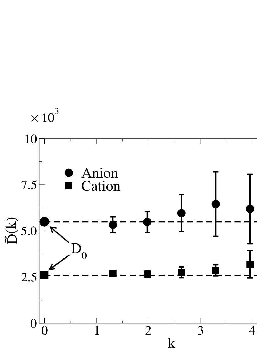
In Fig. 5 (a) the diffusion kernels are is shown for the ion liquid model. These are evaluated as explained in Sect. III.2. One sees that within statistical uncertainty the diffusion kernel is wavevector independent, at least up to $k=5$. Beyond this wavevector value the statistical error increases dramatically and the results are non-conclusive. The charge-charge structure, Fig. 5 (b), is calculated from the direct definition Eq. (24). It features relatively strong structure, that is, the system is in the screening regime. We can therefore expect the response function $\chi$ to resemble low temperature molten salt response function.

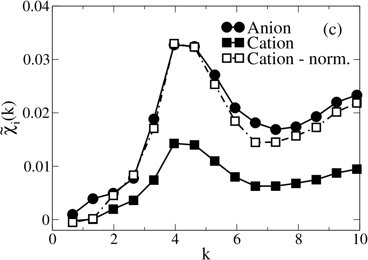
For the ionic liquid Eqs. (13)-(18) do not apply as $\chi_{+}\neq\chi_{-}$ and $D_{+}\neq D_{-}$, and $\widetilde{\chi}_{i}$ is found from non-equilibrium simulations using Eq. (10) directly. This also means that we cannot compare the predictions from these equations with simulation data. The amplitudes of the density profiles for both the anion and cation are analyzed giving $\widetilde{n}_{i}$. Note that only single modes are excited for the low external field applied, $E_{0}=0.05$. Substitution of $\widetilde{n}_{i}$ and $\widetilde{D}=D_{0}$ into Eq. (10) yields the results in Fig. 5 (c). The response features a maximum for $k\approx 4.25$ in good agreement with the maximum charge-charge structure.

To investigate if the two kernels can be mapped onto the same master curve, the results from the cation kernel is normalized with respect the maximum. The normalized result is shown in Fig. 5 (c) as squares connected with a punctured line. To a reasonable agreement the two kernels do follow a master curve which indicates that the underlying mechanisms responsible for the response are the same. This contrasts the wavevector independent diffusion kernel, that is, the system response seen in the mass flux due to the density gradient. Therefore, the physical mechanisms for the two fluxes $j_{i}^{d}$ and $j_{i}^{e}$ are fundamentally different; at least in the screening regime.

References

- [1] J. P. Hansen and I. R. McDonald. Statistical mechanics of dense ionized matter. IV. Density and charge fluctuations in a simple molten salt. Phys. Rev. A, 11:2111, 1975.
- [2] J. P. Hansen and I. R. McDonald. Theory of Simple Liquids. Academic Press, Amsterdam, 2006.
- [3] Stuart Smedley. The interpretation of ionic conductivity in liquids. Plenum Press, 1980.
- [4] K. Harris. Relations between the Fractional Stokes-Einstein and Nernst-Einstein Equations and Velocity Correlation Coefficients in Ionic Liquids and Molten Salts. J. Phys. Chem. B, 114:9572, 2010.
- [5] M. Kanakubo, K.R. Harris, N. Tsuchihashi, K. Ibuki, and M. Ueno. Effect of Pressure on Transport Properties of the Ionic Liquid 1-Butyl-3-methylimidazolium Hexafluorophosphate. J. Chem. Phys. B, 111:2062, 2007.
- [6] K.R. Harris, M. Kanakubo, N. Tsuchihashi, K. Ibuki, and M. Ueno. Effect of Pressure on the Transport Properties of Ionic Liquids: 1-Alkyl-3-methylimidazolium Salts. J. Phys. Chem. B, 112:9830, 2008.
- [7] D. J. Evans and G. P. Morriss. Statistical Mechanics of Nonequilibrium Liquids. Academic Press, 2008.
- [8] J.S. Hansen, J.C. Dyre, P.J. Daivis, B.D. Todd, and H. Bruus. Continuum Nanofluidics. Langmuir, 31:13275, 2015.
- [9] A. Furukawa and H. Tanaka. Nonlocal nature of the viscous transport in supercooled liquids: Complex fluid approach to supercooled liquids. Phys. Rev. Lett., 103:135703, 2009.
- [10] S. R. de Groot and P. Mazur. Non-equilibrium Thermodynamics. Dover Publications, 1984.
- [11] A. Baranyai, D. J. Evans, and P. J. Daivis. Isothermal shear-induced heat-flow. Phys. Rev. A, 46:7593, 1992.
- [12] H. Hoang and G. Galliero. Shear viscosity of inhomogeneous fluids. J. Chem. Phys., 136:124902, 2013.
- [13] B.A. Dalton, P.J. Daivis, J.S. Hansen, and B.D. Todd. Effects of nanoscale density inhomogeneities on shearing fluids. Phys. Rev. E, 88:052143, 2013.
- [14] H. Bruus. Theoretical Microfluidics. Oxford University Press, 2008.
- [15] G.A. Chapela, O. Guzmán, E. Díaz-Herrera, and F. del Rio. Room temperature ionic liquids: A simple model. Effect of chain length and size of intermolecular potential on critical temperature. J. Chem. Phys, 142:154508, 2015.
- [16] C. J. Fennell and J. D. Gezelter. Is the Ewald summation still necessary? Pairwise alternatives to the accecpted standard for long-ranged electrostatics. J. Chem. Phys., 124:234104, 2006.
- [17] J.S. Hansen, T.B. Schrøder, and J.C. Dyre. Simplistic Coulomb forces in Molecular Dynamics: Comparing the Wolf and Shifted-Force Approximations. J. Phys. Chem. B, 116:5738, 2012.
- [18] D. Frenkel and B. Smit. Understanding Molecular Simulation. Academic Press, London, 1996.
- [19] S. Nosé. A molecular dynamics method for simulation in the canonical ensemble. Mol. Phys., 52:255–268, 1984.
- [20] W. G. Hoover. Canonical dynamics: Equilibrium phase-space distributions. Phys. Rev. A, 31:1695–1697, 1985.
- [21] A. Y. Toukmaji and J. A. Board Jr. Ewald summation techniques in perspective: a survey. Comp. Phys. Comm., 95, 1996.
- [22] J. D. Weeks, D. Chandler, and H. C. Andersen. Role of repulsive forces in determining the equilibrium structure of simple liquids. J. Chem. Phys., 54:5237–5247, 1971.
- [23] R. Hayes, G. G. Warr, and R. Atkin. Structure and Nanosctructure in Ionic Liquids. Chem. Rev., 115:6357, 2015.
- [24] J. Sanchez-Badillo, M. Gallo, S. Alvarado, and D. Glossman-Mitnik. Solvation Thermodynamic Properties of Hydrogen Sulfide in [c4mim][pf6], [c44mim][bf4], and [c4mim][cl] Ionic Liquids, Determined by Molecular Simulations. J. Phys. Chem. B, 119:10727, 2015.
- [25] J.P. Boon and S. Yip. Molecular Hydrodynamics. Dover Publication, New York, 1991.