跳到论文正文
W Papers独立论文阅读器 arXiv:1611.02094 论文正文 计算阅读时间 · 0%
引用这篇论文根据当前论文元数据生成,正式投稿前建议核对。


License: arXiv.org perpetual non-exclusive license
arXiv:1611.02094v2 [hep-ph] 10 Nov 2016

Extending two Higgs doublet models for two-loop neutrino mass generation and one-loop neutrinoless double beta decay

Zhen Liu Email: liu-zhen@sjtu.edu.cn Affiliation: Department of Physics and Astronomy, Shanghai Jiao Tong University, 800 Dongchuan Road, Shanghai 200240, China    Pei-Hong Gu Email: peihong.gu@sjtu.edu.cn Affiliation: Department of Physics and Astronomy, Shanghai Jiao Tong University, 800 Dongchuan Road, Shanghai 200240, China
Abstract

We extend some two Higgs doublet models, where the Yukawa couplings for the charged fermion mass generation only involve one Higgs doublet, by two singlet scalars respectively carrying a singly electric charge and a doubly electric charge. The doublet and singlet scalars together can mediate a two-loop diagram to generate a tiny Majorana mass matrix of the standard model neutrinos. Remarkably, the structure of the neutrino mass matrix is fully determined by the symmetric Yukawa couplings of the doubly charged scalar to the right-handed leptons. Meanwhile, a one-loop induced neutrinoless double beta decay can arrive at a testable level even if the electron neutrino has an extremely small Majorana mass. We also study other experimental constraints and implications including some rare processes and Higgs phenomenology.

I Introduction

The massive and mixing neutrinos have been confirmed by the precise measurements on the atmospheric, solar, accelerator and reactor neutrino oscillations [1]. This fact implies the need for new physics beyond the S​U​(3)c×S​U​(2)L×U​(1)YSU(3)_{c}\times SU(2)_{L}\times U(1)_{Y} standard model (SM). On the other hand, the cosmological observations have indicated that the neutrino masses should be in a sub-eV range [1]. In order to understand the small neutrino masses, people have proposed various ideas, among which the tree-level seesaw [2, 3, 4, 5] mechanism is very popular [2, 3, 4, 5, 6, 7, 8, 9, 10, 11, 12]. However, the seesaw will not be easy to verify unless it is not at a naturally high scale. Alternatively, the neutrinos can acquire their tiny masses at loop order [13, 14, 15, 16, 17, 18, 19, 20, 21, 22, 23, 24, 25, 26, 27, 28, 29, 30, 31, 32, 33, 34, 35, 36, 37, 38, 39, 40, 41, 42, 43, 44, 45]. These models for the radiative neutrino mass generation contain additionally charged scalars so that they may be tested at colliders.

In principle the neutrinos can have a Majorana nature [46] since they do not carry any electric charges. One hence can expect a neutrinoless double beta decay (0​ν​β​β0\nu\beta\beta) [47] process mediated by the Majorana electron neutrinos. This 0​ν​β​β0\nu\beta\beta process is determined by one unknown parameter me​em_{ee}, i.e. the −11\!-\!1 element in the Majorana neutrino mass matrix, so that it can be seen in the running and planning experiments unless the me​em_{ee} parameter is big enough [48, 49]. However, there are other possibilities for a 0​ν​β​β0\nu\beta\beta process [5, 10, 50, 51, 52, 53, 54, 55, 56, 57, 58, 59, 60]. For example, some left-right symmetric models for a linear seesaw of tree-level neutrino mass generation can offer a nonconventional tree-level 0​ν​β​β0\nu\beta\beta process with an testable lifetime, which simply depends on the scale of the left-right symmetry breaking rather than the details of the Majorana neutrino mass matrix [61]. One may also consider other models which accommodate an observable 0​ν​β​β0\nu\beta\beta process at tree level and then give a negligible contribution to the neutrino masses at loop order [62]. These 0​ν​β​β0\nu\beta\beta processes, which are related to quite a few arbitrary parameters, thus can be free of the constraint from the neutrino mass matrix [63, 64, 65].

It should be interesting if an enhanced 0​ν​β​β0\nu\beta\beta process originates from a tiny me​em_{ee}. Some people have realized this scenario [37, 38, 39, 40, 41, 42, 43, 44, 45]. In a realistic model [37], after the SM Higgs doublet develops a vacuum expectation value (VEV) for spontaneously breaking the electroweak symmetry, a Higgs triplet without any Yukawa couplings can acquire an induced VEV up to a few GeV, meanwhile, its doubly charged component can mix with a doubly charged scalar singlet. Thanks to the gauge interactions, a two-loop induced Majorana neutrino mass matrix then can have a structure fully determined by the symmetric Yukawa couplings of the doubly charged scalar singlet to the right-handed leptons. As for the 0​ν​β​β0\nu\beta\beta process, it can appear at tree level through the same Yukawa interactions and the related gauge interactions.

In this paper we shall extend some two Higgs doublet models [66], where the Yukawa couplings for the charged fermion mass generation only involve one Higgs scalar, to generate the required neutrino masses and the enhanced 0​ν​β​β0\nu\beta\beta process. Specifically we shall introduce two scalar singlets among which one carries a singly electric charge while the other one carries a doubly electric charge. The singly charged scalar without any Yukawa couplings has a cubic term with the two Higgs scalars. The doubly charged scalar has the Yukawa couplings with the right-handed leptons, besides its trilinear coupling with the singly charged scalar. After the electroweak symmetry breaking, we can obtain a dominant Majorana neutrino mass matrix at two-loop and a negligible one at three-loop level. The symmetric Yukawa couplings of the doubly charged scalar to the right-handed leptons can fully determine the structure of the neutrino mass matrix. The 0​ν​β​β0\nu\beta\beta processes can be induced at tree, one-loop and two-loop level. The amplitudes of these 0​ν​β​β0\nu\beta\beta processes are all proportional to the electron neutrino mass. The one-loop 0​ν​β​β0\nu\beta\beta process can arrive at an observable level even if the electron neutrino mass is extremely small. We will also study other experimental constraints and implications including some rare processes and Higgs phenomenology.

II The models

In the fermion sector, the quarks and leptons are as same as the SM ones,

qL​(3,2,+16)=[uLdL],dR​(3,1,−13),uR​(3,1,+23),lL​(1,2,−12)=[νLeL],eR​(1,1,−1).\displaystyle\begin{array}[]{l}q_{L}(3,2,+\frac{1}{6})\end{array}\!=\!\left[\begin{array}[]{l}u_{L}\\[2.84526pt] d_{L}\end{array}\right],~\begin{array}[]{l}d_{R}(3,1,-\frac{1}{3})\end{array},~\begin{array}[]{l}u_{R}(3,1,+\frac{2}{3})\end{array},~\begin{array}[]{l}l_{L}(1,2,-\frac{1}{2})\end{array}\!=\!\left[\begin{array}[]{l}\nu_{L}\\[2.84526pt] e_{L}\end{array}\right],~\begin{array}[]{l}e_{R}(1,1,-1)\end{array}\,.

Here and thereafter the brackets following the fields describe the transformations under the S​U​(2)c×S​U​(2)L×U​(1)YSU(2)_{c}\times SU(2)_{L}\times U(1)_{Y} gauge groups. The scalar sector contains two charged singlets,

δ±​(1,1,±1),ξ±⁣±​(1,1,±2),\displaystyle\begin{array}[]{l}\delta^{\pm}(1,1,\pm 1)\end{array},~\begin{array}[]{l}\xi^{\pm\pm}(1,1,\pm 2)\end{array}\,,

besides two Higgs doublets,

ϕ1​(1,2,+12)=[ϕ1+ϕ10],ϕ2​(1,2,+12)=[ϕ2+ϕ20].\displaystyle\begin{array}[]{l}\phi_{1}(1,2,+\frac{1}{2})\end{array}\!=\!\left[\begin{array}[]{l}\phi^{+}_{1}\\[5.69054pt] \phi^{0}_{1}\end{array}\right],~\begin{array}[]{l}\phi_{2}(1,2,+\frac{1}{2})\end{array}\!=\!\left[\begin{array}[]{l}\phi^{+}_{2}\\[5.69054pt] \phi^{0}_{2}\end{array}\right]\,.

We impose a softly broken discrete symmetry 𝕊\mathbb{S} so that the Yukawa couplings for generating the charged fermion masses will only involve one Higgs doublet. For example, we can take 𝕊=Z2\mathbb{S}=Z_{2} under which one type or three types of the right-handed fermions and one Higgs scalar carry an odd parity while the other fermions and scalars carry an even parity. Alternatively, the 𝕊\mathbb{S} symmetry can be a global one. For instance, we can take 𝕊=U​(1)X\mathbb{S}=U(1)_{X} under which only one Higgs scalar is non-trivial. We further assume a softly broken lepton number, under which the doubly charged scalar carries a lepton number of two units while the Higgs scalars and the singly charged scalar do not carry any lepton numbers.

We then summarize the allowed Yukawa interactions as below,

  • •

    Case-1: The right-handed up-type quarks, down-type quarks and charged leptons couple to a same Higgs doublet,

    ℒY\displaystyle\mathcal{L}_{Y} =\displaystyle= −yu′​q¯L​ϕ~1​uR−yd′​q¯L​ϕ1​dR−ye′​l¯L​ϕ1​eR−12​f​ξ−⁣−​e¯R​eRc+H.c.​with​f=fT;\displaystyle-y^{\prime}_{u}\bar{q}_{L}\tilde{\phi}_{1}u_{R}-y^{\prime}_{d}\bar{q}_{L}\phi_{1}d_{R}-y^{\prime}_{e}\bar{l}_{L}\phi_{1}e_{R}-\frac{1}{2}f\xi^{--}\bar{e}_{R}e^{c}_{R}+\textrm{H.c.}~~\textrm{with}~~f=f^{T}\,; (21)
  • •

    Case-2: The right-handed up-type quarks and down-type quarks couple to a same Higgs doublet,

    ℒY\displaystyle\mathcal{L}_{Y} =\displaystyle= −yu′​q¯L​ϕ~1​uR−yd′​q¯L​ϕ1​dR−ye′​l¯L​ϕ2​eR−12​f​ξ−⁣−​e¯R​eRc+H.c.​with​f=fT;\displaystyle-y^{\prime}_{u}\bar{q}_{L}\tilde{\phi}_{1}u_{R}-y^{\prime}_{d}\bar{q}_{L}\phi_{1}d_{R}-y^{\prime}_{e}\bar{l}_{L}\phi_{2}e_{R}-\frac{1}{2}f\xi^{--}\bar{e}_{R}e^{c}_{R}+\textrm{H.c.}~~\textrm{with}~~f=f^{T}\,; (22)
  • •

    Case-3: The right-handed up-type quarks and charged leptons couple to a same Higgs doublet,

    ℒY\displaystyle\mathcal{L}_{Y} =\displaystyle= −yu′​q¯L​ϕ~1​uR−yd′​q¯L​ϕ2​dR−ye′​l¯L​ϕ1​eR−12​f​ξ−⁣−​e¯R​eRc+H.c.​with​f=fT;\displaystyle-y^{\prime}_{u}\bar{q}_{L}\tilde{\phi}_{1}u_{R}-y^{\prime}_{d}\bar{q}_{L}\phi_{2}d_{R}-y^{\prime}_{e}\bar{l}_{L}\phi_{1}e_{R}-\frac{1}{2}f\xi^{--}\bar{e}_{R}e^{c}_{R}+\textrm{H.c.}~~\textrm{with}~~f=f^{T}\,; (23)
  • •

    Case-4: The right-handed down-type quarks and charged leptons couple to a same Higgs doublet,

    ℒY\displaystyle\mathcal{L}_{Y} =\displaystyle= −yu′​q¯L​ϕ~1​uR−yd′​q¯L​ϕ2​dR−ye′​l¯L​ϕ2​eR−12​f​ξ−⁣−​e¯R​eRc+H.c.​with​f=fT.\displaystyle-y^{\prime}_{u}\bar{q}_{L}\tilde{\phi}_{1}u_{R}-y^{\prime}_{d}\bar{q}_{L}\phi_{2}d_{R}-y^{\prime}_{e}\bar{l}_{L}\phi_{2}e_{R}-\frac{1}{2}f\xi^{--}\bar{e}_{R}e^{c}_{R}+\textrm{H.c.}~~\textrm{with}~~f=f^{T}\,. (24)

We also write down the full scalar potential with the following quadratic, cubic and quartic terms,

V\displaystyle V =\displaystyle= μ12​|ϕ1|2+μ22​|ϕ2|2+μ122​(ϕ1†​ϕ2+H.c.)+λ1​|ϕ1|4+λ2​|ϕ2|4+λ12​|ϕ1|2​|ϕ2|2+λ12′​ϕ1†​ϕ2​ϕ2†​ϕ1\displaystyle\mu_{1}^{2}|\phi_{1}|^{2}+\mu_{2}^{2}|\phi_{2}|^{2}+\mu_{12}^{2}(\phi^{\dagger}_{1}\phi_{2}+\textrm{H.c.})+\lambda_{1}|\phi_{1}|^{4}+\lambda_{2}|\phi_{2}|^{4}+\lambda_{12}|\phi_{1}|^{2}|\phi_{2}|^{2}+\lambda^{\prime}_{12}\phi_{1}^{\dagger}\phi_{2}\phi_{2}^{\dagger}\phi_{1} (25)
+[λ12′′​(ϕ1†​ϕ2)2+H.c.]+(μδ2+λ1​δ​|ϕ1|2+λ2​δ​|ϕ2|2)​|δ|2+λδ​|δ|4+(μξ2+λ1​ξ​|ϕ1|2+λ2​ξ​|ϕ2|2)​|ξ|2+λξ​|ξ|4\displaystyle+[\lambda^{\prime\prime}_{12}(\phi_{1}^{\dagger}\phi_{2})^{2}+\textrm{H.c.}]+(\mu_{\delta}^{2}+\lambda_{1\delta}|\phi_{1}|^{2}+\lambda_{2\delta}|\phi_{2}|^{2})|\delta|^{2}+\lambda_{\delta}|\delta|^{4}+(\mu_{\xi}^{2}+\lambda_{1\xi}|\phi_{1}|^{2}+\lambda_{2\xi}|\phi_{2}|^{2})|\xi|^{2}+\lambda_{\xi}|\xi|^{4}
+λδ​ξ​|δ|2​|ξ|2+12​ω​(ξ+⁣+​δ−​δ−+H.c.)+σ12​(δ−​ϕ1T​i​τ2​ϕ2+H.c.).\displaystyle+\lambda_{\delta\xi}|\delta|^{2}|\xi|^{2}+\frac{1}{2}\omega(\xi^{++}\delta^{-}\delta^{-}+\textrm{H.c.})+\sigma_{12}(\delta^{-}\phi^{T}_{1}i\tau_{2}\phi_{2}+\textrm{H.c.})\,.

Note only the μ122\mu_{12}^{2}-term, the ω\omega-term and the σ12\sigma_{12}-term can softly break the additional 𝕊\mathbb{S} symmetry. So, if the 𝕊\mathbb{S} symmetry is a global one, the λ12′′\lambda^{\prime\prime}_{12}-term should be absent.

III Electroweak symmetry breaking and physical scalars

The two Higgs scalars ϕ1,2\phi_{1,2} can be always rotated by

χ=[χ+χ0]=ϕ1​cos⁡β−ϕ2​sin⁡β,φ=[φ+φ0]=ϕ1​sin⁡β+ϕ2​cos⁡β.\displaystyle\chi=\left[\begin{array}[]{c}\chi^{+}\\[2.84526pt] \chi^{0}\end{array}\right]=\phi_{1}\cos\beta-\phi_{2}\sin\beta\,,\quad\varphi=\left[\begin{array}[]{c}\varphi^{+}\\[2.84526pt] \varphi^{0}\end{array}\right]=\phi_{1}\sin\beta+\phi_{2}\cos\beta\,.

For a proper choice of the rotation angle β\beta, only one of the newly defined Higgs scalars χ\chi and φ\varphi will develop a nonzero VEV to spontaneously break the electroweak symmetry. Without loss of generality, we can denote

tan⁡β=⟨ϕ1⟩⟨ϕ2⟩=v1v2​with​⟨ϕ1⟩=[012​v1],⟨ϕ2⟩=[012​v2],\displaystyle\tan\beta=\frac{\langle\phi_{1}\rangle}{\langle\phi_{2}\rangle}=\frac{v_{1}}{v_{2}}~~\textrm{with}~~\langle\phi_{1}\rangle=\left[\begin{array}[]{c}0\\[5.69054pt] \frac{1}{\sqrt{2}}v_{1}\end{array}\right]\,,~~\langle\phi_{2}\rangle=\left[\begin{array}[]{c}0\\[5.69054pt] \frac{1}{\sqrt{2}}v_{2}\end{array}\right]\,,

and then take

⟨χ⟩=0,⟨φ⟩=[012​v]​with​v=v12+v22≃246​GeV.\displaystyle\langle\chi\rangle=0\,,\quad\langle\varphi\rangle=\left[\begin{array}[]{c}0\\[5.69054pt] \frac{1}{\sqrt{2}}v\end{array}\right]~~\textrm{with}~~v=\sqrt{v_{1}^{2}+v_{2}^{2}}\simeq 246\,\textrm{GeV}\,.\quad\quad

This means the Higgs scalar φ\varphi will be responsible for the electroweak symmetry breaking.

In the base with ⟨χ⟩=0\langle\chi\rangle=0, we can rewrite the scalar potential to be

V\displaystyle V =\displaystyle= μφ2​|φ|2+Mχ2​|χ|2+κ1​|φ|4+κ2​|χ|4+κ3​|φ|2​|χ|2+κ4​φ†​χ​χ†​φ+κ5​[(φ†​χ)2+H.c.]+(Mδ2+κφ​δ​|φ|2CLOSE\displaystyle\mu_{\varphi}^{2}|\varphi|^{2}+M_{\chi}^{2}|\chi|^{2}+\kappa_{1}|\varphi|^{4}+\kappa_{2}|\chi|^{4}+\kappa_{3}|\varphi|^{2}|\chi|^{2}+\kappa_{4}\varphi^{\dagger}\chi\chi^{\dagger}\varphi+\kappa_{5}[(\varphi^{\dagger}\chi)^{2}+\textrm{H.c.}]+(M_{\delta}^{2}+\kappa_{\varphi\delta}|\varphi|^{2} (39)
OPEN+κχ​δ​|χ|2+κφ​χ​δ​φ†​χ+H.c.)​|δ|2+κδ​|δ|4+(Mξ2+κφ​ξ​|φ|2+κχ​ξ​|χ|2+κφ​χ​ξ​φ†​χ+H.c.)​|ξ|2+κξ​|ξ|4\displaystyle+\kappa_{\chi\delta}|\chi|^{2}+\kappa_{\varphi\chi\delta}\varphi^{\dagger}\chi+\textrm{H.c.})|\delta|^{2}+\kappa_{\delta}|\delta|^{4}+(M_{\xi}^{2}+\kappa_{\varphi\xi}|\varphi|^{2}+\kappa_{\chi\xi}|\chi|^{2}+\kappa_{\varphi\chi\xi}\varphi^{\dagger}\chi+\textrm{H.c.})|\xi|^{2}+\kappa_{\xi}|\xi|^{4}
+κδ​ξ​|δ|2​|ξ|2+12​ω​(ξ+⁣+​δ−​δ−+H.c.)+σ⁡(δ−​φT​i​τ2​χ+H.c.).\displaystyle+\kappa_{\delta\xi}|\delta|^{2}|\xi|^{2}+\frac{1}{2}\omega(\xi^{++}\delta^{-}\delta^{-}+\textrm{H.c.})+\sigma(\delta^{-}\varphi^{T}i\tau_{2}\chi+\textrm{H.c.})\,.

Meanwhile, the Yukawa interactions can be expanded by

  • •

    Case-1:

    ℒY\displaystyle\mathcal{L}_{Y} =\displaystyle= −yu​q¯L​φ~​uR−yd​q¯L​φ​dR−ye​l¯L​φ​eR−(yu​cot⁡β)​q¯L​χ~​uR−(yd​cot⁡β)​q¯L​χ​dR−(ye​cot⁡β)​l¯L​χ​eR\displaystyle-y_{u}\bar{q}_{L}\tilde{\varphi}u_{R}-y_{d}\bar{q}_{L}\varphi d_{R}-y_{e}\bar{l}_{L}\varphi e_{R}-(y_{u}\cot\beta)\bar{q}_{L}\tilde{\chi}u_{R}-(y_{d}\cot\beta)\bar{q}_{L}\chi d_{R}-(y_{e}\cot\beta)\bar{l}_{L}\chi e_{R} (40)
    −12​f​ξ−⁣−​e¯R​eRc+H.c.;\displaystyle-\frac{1}{2}f\xi^{--}\bar{e}_{R}e^{c}_{R}+\textrm{H.c.}\,;
  • •

    Case-2:

    ℒY\displaystyle\mathcal{L}_{Y} =\displaystyle= −yu​q¯L​φ~​uR−yd​q¯L​φ​dR−ye​l¯L​φ​eR−(yu​cot⁡β)​q¯L​χ~​uR−(yd​cot⁡β)​q¯L​χ​dR+(ye​tan⁡β)​l¯L​χ​eR\displaystyle-y_{u}\bar{q}_{L}\tilde{\varphi}u_{R}-y_{d}\bar{q}_{L}\varphi d_{R}-y_{e}\bar{l}_{L}\varphi e_{R}-(y_{u}\cot\beta)\bar{q}_{L}\tilde{\chi}u_{R}-(y_{d}\cot\beta)\bar{q}_{L}\chi d_{R}+(y_{e}\tan\beta)\bar{l}_{L}\chi e_{R} (41)
    −12​f​ξ−⁣−​e¯R​eRc+H.c.;\displaystyle-\frac{1}{2}f\xi^{--}\bar{e}_{R}e^{c}_{R}+\textrm{H.c.}\,;
  • •

    Case-3:

    ℒY\displaystyle\mathcal{L}_{Y} =\displaystyle= −yu​q¯L​φ~​uR−yd​q¯L​φ​dR−ye​l¯L​φ​eR−(yu​cot⁡β)​q¯L​χ~​uR+(yd​tan⁡β)​q¯L​χ​dR−(ye​cot⁡β)​l¯L​χ​eR\displaystyle-y_{u}\bar{q}_{L}\tilde{\varphi}u_{R}-y_{d}\bar{q}_{L}\varphi d_{R}-y_{e}\bar{l}_{L}\varphi e_{R}-(y_{u}\cot\beta)\bar{q}_{L}\tilde{\chi}u_{R}+(y_{d}\tan\beta)\bar{q}_{L}\chi d_{R}-(y_{e}\cot\beta)\bar{l}_{L}\chi e_{R} (42)
    −12​f​ξ−⁣−​e¯R​eRc+H.c.;\displaystyle-\frac{1}{2}f\xi^{--}\bar{e}_{R}e^{c}_{R}+\textrm{H.c.}\,;
  • •

    Case-4:

    ℒY\displaystyle\mathcal{L}_{Y} =\displaystyle= −yu​q¯L​φ~​uR−yd​q¯L​φ​dR−ye​l¯L​φ​eR−(yu​cot⁡β)​q¯L​χ~​uR+(yd​tan⁡β)​q¯L​χ​dR+(ye​tan⁡β)​l¯L​χ​eR\displaystyle-y_{u}\bar{q}_{L}\tilde{\varphi}u_{R}-y_{d}\bar{q}_{L}\varphi d_{R}-y_{e}\bar{l}_{L}\varphi e_{R}-(y_{u}\cot\beta)\bar{q}_{L}\tilde{\chi}u_{R}+(y_{d}\tan\beta)\bar{q}_{L}\chi d_{R}+(y_{e}\tan\beta)\bar{l}_{L}\chi e_{R} (43)
    −12​f​ξ−⁣−​e¯R​eRc+H.c..\displaystyle-\frac{1}{2}f\xi^{--}\bar{e}_{R}e^{c}_{R}+\textrm{H.c.}\,.

After the Higgs scalar φ\varphi develops its VEV for the electroweak symmetry breaking, we can take

φ=[012​(v+h)],χ=[χ+12​(χR0+i​χI0)].\displaystyle\varphi=\left[\begin{array}[]{c}0\\[5.69054pt] \frac{1}{\sqrt{2}}(v+h)\end{array}\right],~~\chi=\left[\begin{array}[]{c}\chi^{+}\\[5.69054pt] \frac{1}{\sqrt{2}}(\chi^{0}_{R}+i\chi^{0}_{I})\end{array}\right]\,.

The scalar potential (39) then should give the mass terms as follows,

V⊃12​mh2​h2+12​mχR02​(χR0)2+12​mχI02​(χI0)2+mχ±2​χ+​χ−+mδ±2​δ+​δ−+mχ±​δ±2​(χ+​δ−+H.c.)+mξ±⁣±2​ξ+⁣+​ξ−⁣−,\displaystyle V\supset\frac{1}{2}m_{h}^{2}h^{2}+\frac{1}{2}m_{\chi^{0}_{R}}^{2}(\chi^{0}_{R})^{2}+\frac{1}{2}m_{\chi^{0}_{I}}^{2}(\chi^{0}_{I})^{2}+m_{\chi^{\pm}}^{2}\chi^{+}\chi^{-}+m_{\delta^{\pm}}^{2}\delta^{+}\delta^{-}+m_{\chi^{\pm}\delta^{\pm}}^{2}(\chi^{+}\delta^{-}+\textrm{H.c.})+m_{\xi^{\pm\pm}}^{2}\xi^{++}\xi^{--}\,, (49)

with

mh2\displaystyle m_{h}^{2} =\displaystyle= 2​κ1​v2=125​GeV,\displaystyle 2\kappa_{1}v^{2}=125\,\textrm{GeV}\,,
mχR02\displaystyle m_{\chi^{0}_{R}}^{2} =\displaystyle= Mχ2+(12​κ3+12​κ4+κ5)​v2>0,\displaystyle M_{\chi}^{2}+\left(\frac{1}{2}\kappa_{3}+\frac{1}{2}\kappa_{4}+\kappa_{5}\right)v^{2}>0\,,
mχI02\displaystyle m_{\chi^{0}_{I}}^{2} =\displaystyle= Mχ2+(12​κ3+12​κ4−κ5)​v2>0,\displaystyle M_{\chi}^{2}+\left(\frac{1}{2}\kappa_{3}+\frac{1}{2}\kappa_{4}-\kappa_{5}\right)v^{2}>0\,,
mχ±2\displaystyle m_{\chi^{\pm}}^{2} =\displaystyle= Mχ2+12​κ3​v2,\displaystyle M_{\chi}^{2}+\frac{1}{2}\kappa_{3}v^{2}\,,
mδ±2\displaystyle m_{\delta^{\pm}}^{2} =\displaystyle= Mδ2+12​κφ​δ​v2,\displaystyle M_{\delta}^{2}+\frac{1}{2}\kappa_{\varphi\delta}v^{2}\,,
mχ±​δ±2\displaystyle m_{\chi^{\pm}\delta^{\pm}}^{2} =\displaystyle= −12​v​σ,\displaystyle-\frac{1}{\sqrt{2}}v\sigma\,,
mξ±⁣±2\displaystyle m_{\xi^{\pm\pm}}^{2} =\displaystyle= Mξ2+12​κφ​ξ​v2>0.\displaystyle M_{\xi}^{2}+\frac{1}{2}\kappa_{\varphi\xi}v^{2}>0\,. (50)

Now the singly charged scalars δ±\delta^{\pm} and χ±\chi^{\pm} mix with each other. Their mass eigenstates should be

χ^±\displaystyle\hat{\chi}^{\pm} =\displaystyle= χ±​cos⁡θ−δ±​sin⁡θ​with​mχ^±2=mχ±2+mδ±2+(mχ±2−mδ±2)2+2​v2​σ22>0,\displaystyle\chi^{\pm}\cos\theta-\delta^{\pm}\sin\theta~~\textrm{with}~~m_{\hat{\chi}^{\pm}}^{2}=\frac{m_{\chi^{\pm}}^{2}+m_{\delta^{\pm}}^{2}+\sqrt{(m_{\chi^{\pm}}^{2}-m_{\delta^{\pm}}^{2})^{2}+2v^{2}\sigma^{2}}}{2}>0\,,
δ^±\displaystyle\hat{\delta}^{\pm} =\displaystyle= χ±​sin⁡θ+δ±​cos⁡θ​with​mδ^±2=mχ±2+mδ±2−(mχ±2−mδ±2)2+2​v2​σ22>0,\displaystyle\chi^{\pm}\sin\theta+\delta^{\pm}\cos\theta~~\textrm{with}~~m_{\hat{\delta}^{\pm}}^{2}=\frac{m_{\chi^{\pm}}^{2}+m_{\delta^{\pm}}^{2}-\sqrt{(m_{\chi^{\pm}}^{2}-m_{\delta^{\pm}}^{2})^{2}+2v^{2}\sigma^{2}}}{2}>0\,, (51)

where the rotation angle θ\theta is determined by

tan⁡2​θ\displaystyle\tan 2\theta =\displaystyle= 2​v​σmχ±2−mδ±2⇒sin2⁡2​θ=2​v2​σ2(mχ^±2−mδ^±2)2=2​(v2mξ±⁣±2)​(σ2mξ±⁣±2)(mχ^±2mξ±⁣±2−mδ^±2mξ±⁣±2)2≤1​for\displaystyle\frac{\sqrt{2}v\sigma}{m_{\chi^{\pm}}^{2}-m_{\delta^{\pm}}^{2}}\Rightarrow\sin^{2}2\theta=\frac{2v^{2}\sigma^{2}}{(m_{\hat{\chi}^{\pm}}^{2}-m_{\hat{\delta}^{\pm}}^{2})^{2}}=\frac{2\left(\frac{v^{2}}{m_{\xi^{\pm\pm}}^{2}}\right)\left(\frac{\sigma^{2}}{m_{\xi^{\pm\pm}}^{2}}\right)}{\left(\frac{m_{\hat{\chi}^{\pm}}^{2}}{m_{\xi^{\pm\pm}}^{2}}-\frac{m_{\hat{\delta}^{\pm}}^{2}}{m_{\xi^{\pm\pm}}^{2}}\right)^{2}}\leq 1~~\textrm{for}
Δ​m±2\displaystyle\Delta m_{\pm}^{2} ≡\displaystyle\equiv mχ^±2−mδ^±2=(mχ±2−mδ±2)2+2​v2​σ2≥2​v​|σ|.\displaystyle m_{\hat{\chi}^{\pm}}^{2}-m_{\hat{\delta}^{\pm}}^{2}=\sqrt{(m_{\chi^{\pm}}^{2}-m_{\delta^{\pm}}^{2})^{2}+2v^{2}\sigma^{2}}\geq\sqrt{2}v|\sigma|\,. (52)

The charged fermions can get their masses through the Yukawa couplings involving the Higgs scalar φ\varphi, i.e. [1]

m^u\displaystyle\hat{m}_{u} =\displaystyle= v2​y^u=diag​{mu,mc,mt}≃diag​{2.2​MeV,1.27​GeV,173​GeV},\displaystyle\frac{v}{\sqrt{2}}\hat{y}_{u}=\textrm{diag}\{m_{u},~m_{c},~m_{t}\}\simeq\textrm{diag}\{2.2\,\textrm{MeV},~1.27\,\textrm{GeV},~173\,\textrm{GeV}\}\,,
m^d\displaystyle\hat{m}_{d} =\displaystyle= v2​y^d=diag​{md,ms,mb}≃diag​{4.7​MeV,96​MeV,4.18​GeV},\displaystyle\frac{v}{\sqrt{2}}\hat{y}_{d}=\textrm{diag}\{m_{d},~m_{s},~m_{b}\}\simeq\textrm{diag}\{4.7\,\textrm{MeV},~96\,\textrm{MeV}\,,~4.18\,\textrm{GeV}\}\,,
m^e\displaystyle\hat{m}_{e} =\displaystyle= v2​y^e=diag​{me,mμ,mτ}≃diag​{0.511​MeV,107​MeV,1.78​GeV}.\displaystyle\frac{v}{\sqrt{2}}\hat{y}_{e}=\textrm{diag}\{m_{e},~m_{\mu},~m_{\tau}\}\simeq\textrm{diag}\{0.511\,\textrm{MeV},~107\,\textrm{MeV},~1.78\,\textrm{GeV}\}\,. (53)

Note the perturbation requirement |y^t′|<4​π|\hat{y}^{\prime}_{t}|<\sqrt{4\pi}, |y^b′|<4​π|\hat{y}^{\prime}_{b}|<\sqrt{4\pi} and |y^τ′|<4​π|\hat{y}^{\prime}_{\tau}|<\sqrt{4\pi} will constrain,

  • •

    Case-1:

    cot⁡β≲3.3​for​cot⁡β<2​π​v2mt2−1;\displaystyle\cot\beta\lesssim 3.3~~\textrm{for}~~\cot\beta<\sqrt{\frac{2\pi v^{2}}{m_{t}^{2}}-1}\,; (54)
  • •

    Case-2:

    0.3≲tan⁡β≲346​for​12​π​v2mt2−1<tan⁡β<2​π​v2mτ2−1;\displaystyle 0.3\lesssim\tan\beta\lesssim 346~~\textrm{for}~~\frac{1}{\sqrt{\frac{2\pi v^{2}}{m_{t}^{2}}-1}}<\tan\beta<\sqrt{\frac{2\pi v^{2}}{m_{\tau}^{2}}-1}\,; (55)
  • •

    Case-3:

    6.8×10⁻³≲cot⁡β≲3.3​for​12​π​v2mb2−1<cot⁡β<2​π​v2mt2−1;\displaystyle 6.8\times 10^{-3}\lesssim\cot\beta\lesssim 3.3~~\textrm{for}~~\frac{1}{\sqrt{\frac{2\pi v^{2}}{m_{b}^{2}}-1}}<\cot\beta<\sqrt{\frac{2\pi v^{2}}{m_{t}^{2}}-1}\,; (56)
  • •

    Case-4:

    0.3≲tan⁡β≲147​for​12​π​v2mt2−1<tan⁡β<2​π​v2mb2−1.\displaystyle 0.3\lesssim\tan\beta\lesssim 147~~\textrm{for}~~\frac{1}{\sqrt{\frac{2\pi v^{2}}{m_{t}^{2}}-1}}<\tan\beta<\sqrt{\frac{2\pi v^{2}}{m_{b}^{2}}-1}\,. (57)

Moreover, the cubic couplings ω\omega and σ\sigma in the potential (39) should also match the perturbation requirement. Roughly speaking, we have

ω≲max​{Mξ,Mδ},σ≲max​{Mδ,Mχ}.\displaystyle\omega\lesssim\textrm{max}\{M_{\xi},~M_{\delta}\}\,,~~\sigma\lesssim\textrm{max}\{M_{\delta},~M_{\chi}\}\,. (58)

IV Neutrino masses

Refer to caption
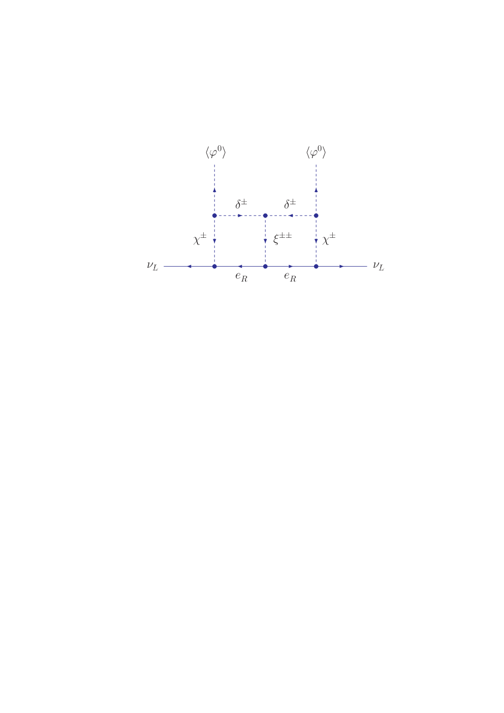
Figure 1: Two-loop diagram for Majorana neutrino masses.
Refer to caption
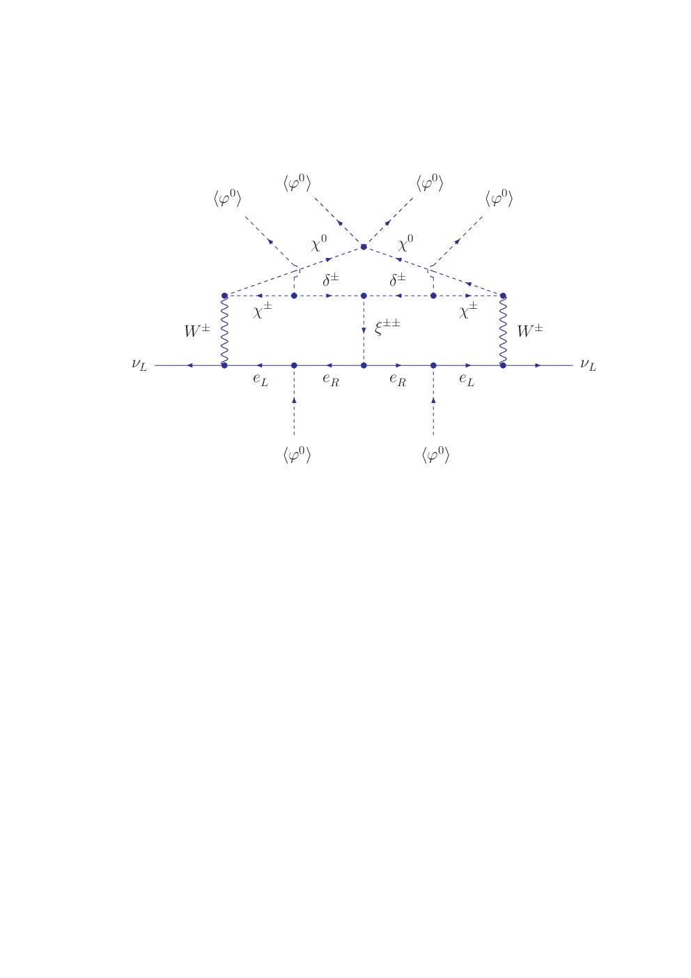
Figure 2: Three-loop diagram for Majorana neutrino masses.

As shown in Fig. 1, the left-handed neutrinos can obtain a Majorana mass term at two-loop level,

ℒ\displaystyle\mathcal{L} ⊃\displaystyle\supset −12​mν​ν¯L​νLc+H.c..\displaystyle-\frac{1}{2}m_{\nu}\bar{\nu}_{L}\nu_{L}^{c}+\textrm{H.c.}\,. (59)

It is easy to see that the two-loop neutrino mass matrix should have the structure as follows,

mν2-loop∝y^e​f​y^e∝m^e​f​m^e.\displaystyle m_{\nu}^{\textrm{2-loop}}\propto\hat{y}_{e}f\hat{y}_{e}\propto\hat{m}_{e}f\hat{m}_{e}\,. (60)

Although the three-loop diagram given in Fig. 2 also generates the neutrino masses,

mν3-loop∝m^e​f​m^e,\displaystyle m_{\nu}^{\textrm{3-loop}}\propto\hat{m}_{e}f\hat{m}_{e}\,, (61)

its contribution should be much smaller than the two-loop contribution (60). So, the neutrino mass matrix can be well described by

mν≃mν2-loop≫mν3-loop.\displaystyle m_{\nu}\simeq m_{\nu}^{\textrm{2-loop}}\gg m_{\nu}^{\textrm{3-loop}}\,. (62)
Refer to caption
Figure 3: The two-loop integral I2​(x12,x22)I_{2}(x_{1}^{2},x_{2}^{2}) as a function of the difference x2−x1x_{2}-x_{1} for a given x1x_{1}. The lines from top to bottom correspond to x1=0.1x_{1}=0.1, x1=1x_{1}=1, x1=10x_{1}=10 and x1=100x_{1}=100, respectively.

We calculate

mν=c​I2​sin2⁡2​θ2​(16​π2)2​y^e​f​y^e​ω=c​I2​sin2⁡2​θ28​π4​m^e​f​m^ev2​ωwithc={cot2⁡βin​​C​a​s​e−1,3,tan2⁡βin​​C​a​s​e−2,4.\displaystyle m_{\nu}=\frac{cI_{2}\sin^{2}2\theta}{2(16\pi^{2})^{2}}\hat{y}_{e}f\hat{y}_{e}\omega=\frac{cI_{2}\sin^{2}2\theta}{2^{8}\pi^{4}}\frac{\hat{m}_{e}f\hat{m}_{e}}{v^{2}}\omega\quad\textrm{with}\quad c=\left\{\begin{array}[]{ll}\cot^{2}\beta&\textrm{in}~\emph{Case-1,3}\,,\\[5.69054pt] \tan^{2}\beta&\textrm{in}~\emph{Case-2,4}\,.\end{array}\right.

Here I2I_{2} is given by the two-loop integral,

I2​(mδ^±2mξ±⁣±2,mχ^±2mξ±⁣±2)\displaystyle I_{2}\left(\frac{m_{\hat{\delta}^{\pm}}^{2}}{m_{\xi^{\pm\pm}}^{2}},\frac{m_{\hat{\chi}^{\pm}}^{2}}{m_{\xi^{\pm\pm}}^{2}}\right)\! =\displaystyle= F2​(mδ^±2mξ±⁣±2,mδ^±2mξ±⁣±2)+F2​(mχ^±2mξ±⁣±2,mχ^±2mξ±⁣±2)−2​F2​(mχ^±2mξ±⁣±2,mδ^±2mξ±⁣±2),\displaystyle\!F_{2}\left(\frac{m_{\hat{\delta}^{\pm}}^{2}}{m_{\xi^{\pm\pm}}^{2}},\frac{m_{\hat{\delta}^{\pm}}^{2}}{m_{\xi^{\pm\pm}}^{2}}\right)+F_{2}\left(\frac{m_{\hat{\chi}^{\pm}}^{2}}{m_{\xi^{\pm\pm}}^{2}},\frac{m_{\hat{\chi}^{\pm}}^{2}}{m_{\xi^{\pm\pm}}^{2}}\right)-2F_{2}\left(\frac{m_{\hat{\chi}^{\pm}}^{2}}{m_{\xi^{\pm\pm}}^{2}},\frac{m_{\hat{\delta}^{\pm}}^{2}}{m_{\xi^{\pm\pm}}^{2}}\right)\,, (66)

where the function F2​(x12,x22)F_{2}(x_{1}^{2},x_{2}^{2}) is defined by

F2​(x12,x22)=(16​π2)2​∫d4​q~1(2​π)4​d4​q~2(2​π)4​/q~1/q~2q~12​(q~12−x12)​q~22​(q~22−x22)​[(q~1+q~2)2−1],\displaystyle F_{2}(x_{1}^{2},x_{2}^{2})=(16\pi^{2})^{2}\int\frac{d^{4}\tilde{q}_{1}}{(2\pi)^{4}}\frac{d^{4}\tilde{q}_{2}}{(2\pi)^{4}}\frac{/\!\!\!\tilde{q}_{1}/\!\!\!\tilde{q}_{2}}{\tilde{q}_{1}^{2}(\tilde{q}_{1}^{2}-x_{1}^{2})\tilde{q}_{2}^{2}(\tilde{q}_{2}^{2}-x_{2}^{2})[(\tilde{q}_{1}+\tilde{q}_{2})^{2}-1]}\,, (67)

with q~1,2=q1,2/mξ±⁣±\tilde{q}_{1,2}=q_{1,2}/m_{\xi^{\pm\pm}} being the reduced momentum.

In Fig. 3, we show the numerical results of the two-loop integral I2​(x12,x22)I_{2}(x_{1}^{2},x_{2}^{2}) as a function of the difference x2−x1x_{2}-x_{1} for a given x1x_{1}. The lines from top to bottom correspond to x1=0.1x_{1}=0.1, x1=1x_{1}=1, x1=10x_{1}=10 and x1=100x_{1}=100, respectively. For a proper parameter choice, the two-loop integral I2I_{2} can be of the order of 𝒪⁡(1)\mathcal{O}(1). Note that I2​(x12,x22)≡0I_{2}(x_{1}^{2},x_{2}^{2})\equiv 0 for x1=x2x_{1}=x_{2}. We should also keep in mind that a bigger x2−x1x_{2}-x_{1} leads to a bigger I2I_{2} but a smaller sin2⁡2​θ\sin^{2}2\theta, see Eq. (52). The product I2​sin2⁡2​θI_{2}\sin^{2}2\theta thus cannot be very large. We hence would fail in enhancing the neutrino masses by choosing a bigger cubic coupling ω\omega, which is not allowed to be much bigger than the charged scalar masses. In other words, the charged scalars cannot be far above the electroweak scale.

Now the neutrino mass matrix has a structure fully determined by the symmetric Yukawa couplings fα​β=fβ​αf_{\alpha\beta}=f_{\beta\alpha} (α,β=e,μ,τ)(\alpha,\beta=e,\mu,\tau), i.e.

mα​β\displaystyle\!\!\!\!m_{\alpha\beta} ≡\displaystyle\equiv (mν)α​β=c​I2​sin2⁡2​θ28​π4​ω​mα​mβv2​fα​β.\displaystyle(m_{\nu})_{\alpha\beta}=\frac{cI_{2}\sin^{2}2\theta}{2^{8}\pi^{4}}\frac{\omega m_{\alpha}m_{\beta}}{v^{2}}f_{\alpha\beta}\,. (68)

Actually we read

me​e\displaystyle m_{ee} =\displaystyle= 6×10⁻⁴​eV​(fe​e4​π)​(c1)​(I21)​(sin2⁡2​θ1)​(ω1​TeV),\displaystyle 6\times 10^{-4}\,\textrm{eV}\left(\frac{f_{ee}}{\sqrt{4\pi}}\right)\left(\frac{c}{1}\right)\left(\frac{I_{2}}{1}\right)\left(\frac{\sin^{2}2\theta}{1}\right)\left(\frac{\omega}{1\,\textrm{TeV}}\right)\,,
mμ​μ\displaystyle m_{\mu\mu} =\displaystyle= 0.1​eV​(fμ​μ0.013)​(c1)​(I21)​(sin2⁡2​θ1)​(ω1​TeV),\displaystyle 0.1\,\textrm{eV}\left(\frac{f_{\mu\mu}}{0.013}\right)\left(\frac{c}{1}\right)\left(\frac{I_{2}}{1}\right)\left(\frac{\sin^{2}2\theta}{1}\right)\left(\frac{\omega}{1\,\textrm{TeV}}\right)\,,
mτ​τ\displaystyle m_{\tau\tau} =\displaystyle= 0.1​eV​(fτ​τ5×10⁻⁵)​(c1)​(I21)​(sin2⁡2​θ1)​(ω1​TeV),\displaystyle 0.1\,\textrm{eV}\left(\frac{f_{\tau\tau}}{5\times 10^{-5}}\right)\left(\frac{c}{1}\right)\left(\frac{I_{2}}{1}\right)\left(\frac{\sin^{2}2\theta}{1}\right)\left(\frac{\omega}{1\,\textrm{TeV}}\right)\,,
me​μ\displaystyle m_{e\mu} =\displaystyle= mμ​e=0.1​eV​(fe​μ2.9)​(c1)​(I21)​(sin2⁡2​θ1)​(ω1​TeV),\displaystyle m_{\mu e}=0.1\,\textrm{eV}\left(\frac{f_{e\mu}}{2.9}\right)\left(\frac{c}{1}\right)\left(\frac{I_{2}}{1}\right)\left(\frac{\sin^{2}2\theta}{1}\right)\left(\frac{\omega}{1\,\textrm{TeV}}\right)\,,
me​τ\displaystyle m_{e\tau} =\displaystyle= mτ​e=0.1​eV​(fe​τ0.17)​(c1)​(I21)​(sin2⁡2​θ1)​(ω1​TeV),\displaystyle m_{\tau e}=0.1\,\textrm{eV}\left(\frac{f_{e\tau}}{0.17}\right)\left(\frac{c}{1}\right)\left(\frac{I_{2}}{1}\right)\left(\frac{\sin^{2}2\theta}{1}\right)\left(\frac{\omega}{1\,\textrm{TeV}}\right)\,,
mμ​τ\displaystyle m_{\mu\tau} =\displaystyle= mτ​μ=0.1​eV​(fμ​τ8×10⁻⁴)​(c1)​(I21)​(sin2⁡2​θ1)​(ω1​TeV).\displaystyle m_{\tau\mu}=0.1\,\textrm{eV}\left(\frac{f_{\mu\tau}}{8\times 10^{-4}}\right)\left(\frac{c}{1}\right)\left(\frac{I_{2}}{1}\right)\left(\frac{\sin^{2}2\theta}{1}\right)\left(\frac{\omega}{1\,\textrm{TeV}}\right)\,. (69)

In turn, we can parametrize the Yukawa couplings ff by the neutrino mass matrix,

f\displaystyle f =\displaystyle= 28​π4​v2c​I2​sin2⁡2​θ​1m^e​mν​1m^e​1ω.\displaystyle\frac{2^{8}\pi^{4}v^{2}}{cI_{2}\sin^{2}2\theta}\frac{1}{\hat{m}_{e}}m_{\nu}\frac{1}{\hat{m}_{e}}\frac{1}{\omega}\,. (70)

V Neutrinoless double beta decay

It is well known that the electron neutrino with a Majorana mass can mediate a 0​ν​β​β0\nu\beta\beta process. This most popular 0​ν​β​β0\nu\beta\beta picture can be described by the effective operator as below,

𝒪2-loop\displaystyle\mathcal{O}^{\textrm{2-loop}} =\displaystyle= g42​mW4​u¯L​γμ​dL​u¯L​γν​dL​e¯L​γμ​γν​eLc​me​eq2=1Λ25​u¯L​γμ​dL​u¯L​γν​dL​e¯L​γμ​γν​eLc​with​1Λ25=16​GF2​me​eq2,\displaystyle\frac{g^{4}}{2m_{W}^{4}}\bar{u}_{L}\gamma^{\mu}d_{L}\bar{u}_{L}\gamma^{\nu}d_{L}\bar{e}_{L}\gamma_{\mu}\gamma_{\nu}e_{L}^{c}\frac{m_{ee}}{q^{2}}=\frac{1}{\Lambda_{2}^{5}}\bar{u}_{L}\gamma^{\mu}d_{L}\bar{u}_{L}\gamma^{\nu}d_{L}\bar{e}_{L}\gamma_{\mu}\gamma_{\nu}e_{L}^{c}~~\textrm{with}~~\frac{1}{\Lambda_{2}^{5}}=16\,G_{F}^{2}\frac{m_{ee}}{q^{2}}\,, (71)

where q=100−200​MeVq=100-200\,\textrm{MeV} is the transfer momentum. In the present model, the above 0​ν​β​β0\nu\beta\beta process actually is a two-loop effect since the neutrino masses are induced at two-loop level.

Refer to caption
Figure 4: Tree and one-loop diagrams for neutrinoless double beta decay.

As shown in Figs. 4a, our model can also generate the other 0​ν​β​β0\nu\beta\beta processes at tree level. The effective operators should be

𝒪tree\displaystyle\mathcal{O}^{\textrm{tree}} =\displaystyle= 1Λ015​u¯L​dR​u¯L​dR​e¯Rc​eR+1Λ025​u¯R​dL​u¯R​dL​e¯Rc​eR+1Λ035​u¯L​dR​u¯R​dL​e¯Rc​eR​with\displaystyle\frac{1}{\Lambda_{01}^{5}}\bar{u}_{L}d_{R}\bar{u}_{L}d_{R}\bar{e}_{R}^{c}e_{R}+\frac{1}{\Lambda_{02}^{5}}\bar{u}_{R}d_{L}\bar{u}_{R}d_{L}\bar{e}_{R}^{c}e_{R}+\frac{1}{\Lambda_{03}^{5}}\bar{u}_{L}d_{R}\bar{u}_{R}d_{L}\bar{e}_{R}^{c}e_{R}~~\textrm{with}
1Λ015\displaystyle\frac{1}{\Lambda_{01}^{5}} =\displaystyle= 14​y^d2​fe​e​c1​sin2⁡2​θ​ωmξ±⁣±2​(1mχ^±2−1mδ^±2)2=27​π4I2​c1c​md2me2​me​e​Δ​m±2mξ±⁣±2​mχ^±2​mδ^±2\displaystyle\frac{1}{4}\hat{y}_{d}^{2}f_{ee}c_{1}\sin^{2}2\theta\frac{\omega}{m^{2}_{\xi^{\pm\pm}}}\left(\frac{1}{m_{\hat{\chi}^{\pm}}^{2}}-\frac{1}{m_{\hat{\delta}^{\pm}}^{2}}\right)^{2}=\frac{2^{7}\pi^{4}}{I_{2}}\frac{c_{1}}{c}\frac{m_{d}^{2}}{m_{e}^{2}}\frac{m_{ee}\Delta m_{\pm}^{2}}{m^{2}_{\xi^{\pm\pm}}m_{\hat{\chi}^{\pm}}^{2}m_{\hat{\delta}^{\pm}}^{2}}
=\displaystyle= 2×(c1c)​(md3​MeV)2​(q100​MeV)2​(Δ​m±21​TeV2)​(1​TeVmξ±⁣±)2​(1​TeVmχ^±)2​(1​TeVmδ^±)2​1Λ25,\displaystyle 2\times\left(\frac{c_{1}}{c}\right)\left(\frac{m_{d}}{3\,\textrm{MeV}}\right)^{2}\left(\frac{q}{100\,\textrm{MeV}}\right)^{2}\left(\frac{\Delta m_{\pm}^{2}}{1\,\textrm{TeV}^{2}}\right)\left(\frac{1\,\textrm{TeV}}{m_{\xi^{\pm\pm}}}\right)^{2}\left(\frac{1\,\textrm{TeV}}{m_{\hat{\chi}^{\pm}}}\right)^{2}\left(\frac{1\,\textrm{TeV}}{m_{\hat{\delta}^{\pm}}}\right)^{2}\frac{1}{\Lambda_{2}^{5}}\,,
1Λ025\displaystyle\frac{1}{\Lambda_{02}^{5}} =\displaystyle= 14​y^u2​fe​e​c2​sin2⁡2​θ​ωmξ±⁣±2​(1mχ^±2−1mδ^±2)2=27​π4I2​c2c​mu2me2​me​e​Δ​m±2mξ±⁣±2​mχ^±2​mδ^±2\displaystyle\frac{1}{4}\hat{y}_{u}^{2}f_{ee}c_{2}\sin^{2}2\theta\frac{\omega}{m^{2}_{\xi^{\pm\pm}}}\left(\frac{1}{m_{\hat{\chi}^{\pm}}^{2}}-\frac{1}{m_{\hat{\delta}^{\pm}}^{2}}\right)^{2}=\frac{2^{7}\pi^{4}}{I_{2}}\frac{c_{2}}{c}\frac{m_{u}^{2}}{m_{e}^{2}}\frac{m_{ee}\Delta m_{\pm}^{2}}{m^{2}_{\xi^{\pm\pm}}m_{\hat{\chi}^{\pm}}^{2}m_{\hat{\delta}^{\pm}}^{2}}
=\displaystyle= 0.5×(c2c)​(mu1.5​MeV)2​(q100​MeV)2​(Δ​m±21​TeV2)​(1​TeVmξ±⁣±)2​(1​TeVmχ^±)2​(1​TeVmδ^±)2​1Λ25,\displaystyle 0.5\times\left(\frac{c_{2}}{c}\right)\left(\frac{m_{u}}{1.5\,\textrm{MeV}}\right)^{2}\left(\frac{q}{100\,\textrm{MeV}}\right)^{2}\left(\frac{\Delta m_{\pm}^{2}}{1\,\textrm{TeV}^{2}}\right)\left(\frac{1\,\textrm{TeV}}{m_{\xi^{\pm\pm}}}\right)^{2}\left(\frac{1\,\textrm{TeV}}{m_{\hat{\chi}^{\pm}}}\right)^{2}\left(\frac{1\,\textrm{TeV}}{m_{\hat{\delta}^{\pm}}}\right)^{2}\frac{1}{\Lambda_{2}^{5}}\,,
1Λ035\displaystyle\frac{1}{\Lambda_{03}^{5}} =\displaystyle= 14​y^d​y^u​fe​e​c3​sin2⁡2​θ​ωmξ±⁣±2​(1mχ^±2−1mδ^±2)2=27​π4I2​c3c​md​mume2​me​e​Δ​m±2mξ±⁣±2​mχ^±2​mδ^±2\displaystyle\frac{1}{4}\hat{y}_{d}\hat{y}_{u}f_{ee}c_{3}\sin^{2}2\theta\frac{\omega}{m^{2}_{\xi^{\pm\pm}}}\left(\frac{1}{m_{\hat{\chi}^{\pm}}^{2}}-\frac{1}{m_{\hat{\delta}^{\pm}}^{2}}\right)^{2}=\frac{2^{7}\pi^{4}}{I_{2}}\frac{c_{3}}{c}\frac{m_{d}m_{u}}{m_{e}^{2}}\frac{m_{ee}\Delta m_{\pm}^{2}}{m^{2}_{\xi^{\pm\pm}}m_{\hat{\chi}^{\pm}}^{2}m_{\hat{\delta}^{\pm}}^{2}} (72)
=\displaystyle= 1×(c3c)​(md3​MeV)​(mu1.5​MeV)​(q100​MeV)2​(Δ​m±21​TeV2)​(1​TeVmξ±⁣±)2​(1​TeVmχ^±)2​(1​TeVmδ^±)2​1Λ25,\displaystyle 1\times\left(\frac{c_{3}}{c}\right)\left(\frac{m_{d}}{3\,\textrm{MeV}}\right)\left(\frac{m_{u}}{1.5\,\textrm{MeV}}\right)\left(\frac{q}{100\,\textrm{MeV}}\right)^{2}\left(\frac{\Delta m_{\pm}^{2}}{1\,\textrm{TeV}^{2}}\right)\left(\frac{1\,\textrm{TeV}}{m_{\xi^{\pm\pm}}}\right)^{2}\left(\frac{1\,\textrm{TeV}}{m_{\hat{\chi}^{\pm}}}\right)^{2}\left(\frac{1\,\textrm{TeV}}{m_{\hat{\delta}^{\pm}}}\right)^{2}\frac{1}{\Lambda_{2}^{5}}\,,

where the coefficients c1,2,3c_{1,2,3} are defined by

(c1,c2,c3)={(c,c,c)in​​C​a​s​e−1,(1c,1c,1c)in​​C​a​s​e−2,(1c,c,1)in​​C​a​s​e−3,(c,1c,1)in​​C​a​s​e−4.\displaystyle(c_{1},c_{2},c_{3})=\left\{\begin{array}[]{ll}(c,c,c)&\textrm{in}~\emph{Case-1}\,,\\[5.69054pt] (\frac{1}{c},\frac{1}{c},\frac{1}{c})&\textrm{in}~\emph{Case-2}\,,\\[5.69054pt] (\frac{1}{c},c,1)&\textrm{in}~\emph{Case-3}\,,\\[5.69054pt] (c,\frac{1}{c},1)&\textrm{in}~\emph{Case-4}\,.\\[5.69054pt] \end{array}\right.
Refer to caption
Figure 5: The one-loop integral I~1​(x12,x22)≡I1​R​(x12,x22)\tilde{I}_{1}(x_{1}^{2},x_{2}^{2})\equiv I_{1R}(x_{1}^{2},x_{2}^{2}) or I~1​(x12,x22)≡I1​I​(x12,x22)\tilde{I}_{1}(x_{1}^{2},x_{2}^{2})\equiv I_{1I}(x_{1}^{2},x_{2}^{2}) as a function of the difference x2−x1x_{2}-x_{1} for a given x1x_{1}. The lines from top to bottom correspond to x1=0.1x_{1}=0.1, x1=1x_{1}=1, x1=10x_{1}=10 and x1=100x_{1}=100, respectively.

Furthermore, we can realize a 0​ν​β​β0\nu\beta\beta process at one-loop level. The relevant diagram is shown in Fig. 4b. The effective operator should be

𝒪1-loop\displaystyle\mathcal{O}^{\textrm{1-loop}} =\displaystyle= 1Λ15​u¯L​γμ​dL​u¯L​γμ​dL​e¯R​eRc​with\displaystyle\frac{1}{\Lambda_{1}^{5}}\bar{u}_{L}\gamma^{\mu}d_{L}\bar{u}_{L}\gamma_{\mu}d_{L}\bar{e}_{R}e_{R}^{c}~~\textrm{with}
1Λ15\displaystyle\frac{1}{\Lambda_{1}^{5}} =\displaystyle= 127​π2​g4mW4​ωmξ±⁣±2​fe​e​I1​sin2⁡2​θ=64​π2​GF2​v2mξ±⁣±2​me​eme2​I1I2​1c\displaystyle\frac{1}{2^{7}\pi^{2}}\frac{g^{4}}{m_{W}^{4}}\frac{\omega}{m^{2}_{\xi^{\pm\pm}}}f_{ee}I_{1}\sin^{2}2\theta=64\,\pi^{2}\,G_{F}^{2}\frac{v^{2}}{m_{\xi^{\pm\pm}}^{2}}\frac{m_{ee}}{m_{e}^{2}}\frac{I_{1}}{I_{2}}\frac{1}{c} (78)
=\displaystyle= 9×10⁴×(q100​MeV)2​(1​TeVmξ±⁣±)2​(I11)​(1I2)​(1c)​1Λ25.\displaystyle 9\times 10^{4}\times\left(\frac{q}{100\,\textrm{MeV}}\right)^{2}\left(\frac{1\,\textrm{TeV}}{m_{\xi^{\pm\pm}}}\right)^{2}\left(\frac{I_{1}}{1}\right)\left(\frac{1}{I_{2}}\right)\left(\frac{1}{c}\right)\frac{1}{\Lambda_{2}^{5}}\,.

Here I1I_{1} is given by the one-loop integral,

I1\displaystyle I_{1} =\displaystyle= I1​R​(mχ^±2mχR02,mδ^±2mχR02)−I1​I​(mχ^±2mχI02,mδ^±2mχI02),\displaystyle I_{1R}\left(\frac{m_{\hat{\chi}^{\pm}}^{2}}{m_{\chi^{0}_{R}}^{2}},\frac{m_{\hat{\delta}^{\pm}}^{2}}{m_{\chi^{0}_{R}}^{2}}\right)-I_{1I}\left(\frac{m_{\hat{\chi}^{\pm}}^{2}}{m_{\chi^{0}_{I}}^{2}},\frac{m_{\hat{\delta}^{\pm}}^{2}}{m_{\chi^{0}_{I}}^{2}}\right)\,,
I1​R​(mχ^±2mχR02,mδ^±2mχR02)\displaystyle I_{1R}\left(\frac{m_{\hat{\chi}^{\pm}}^{2}}{m_{\chi^{0}_{R}}^{2}},\frac{m_{\hat{\delta}^{\pm}}^{2}}{m_{\chi^{0}_{R}}^{2}}\right) =\displaystyle= F1​(mχ^±2mχR02,mχ^±2mχR02)+F1​(mδ^±2mχR02,mδ^±2mχR02)−2​F1​(mχ^±2mχR02,mδ^±2mχR02),\displaystyle F_{1}\left(\frac{m_{\hat{\chi}^{\pm}}^{2}}{m_{\chi^{0}_{R}}^{2}},\frac{m_{\hat{\chi}^{\pm}}^{2}}{m_{\chi^{0}_{R}}^{2}}\right)+F_{1}\left(\frac{m_{\hat{\delta}^{\pm}}^{2}}{m_{\chi^{0}_{R}}^{2}},\frac{m_{\hat{\delta}^{\pm}}^{2}}{m_{\chi^{0}_{R}}^{2}}\right)-2F_{1}\left(\frac{m_{\hat{\chi}^{\pm}}^{2}}{m_{\chi^{0}_{R}}^{2}},\frac{m_{\hat{\delta}^{\pm}}^{2}}{m_{\chi^{0}_{R}}^{2}}\right)\,,
I1​I​(mχ^±2mχI02,mδ^±2mχI02)\displaystyle I_{1I}\left(\frac{m_{\hat{\chi}^{\pm}}^{2}}{m_{\chi^{0}_{I}}^{2}},\frac{m_{\hat{\delta}^{\pm}}^{2}}{m_{\chi^{0}_{I}}^{2}}\right) =\displaystyle= F1​(mχ^±2mχI02,mχ^±2mχI02)+F1​(mδ^±2mχI02,mδ^±2mχI02)−2​F1​(mχ^±2mχI02,mδ^±2mχI02),\displaystyle F_{1}\left(\frac{m_{\hat{\chi}^{\pm}}^{2}}{m_{\chi^{0}_{I}}^{2}},\frac{m_{\hat{\chi}^{\pm}}^{2}}{m_{\chi^{0}_{I}}^{2}}\right)+F_{1}\left(\frac{m_{\hat{\delta}^{\pm}}^{2}}{m_{\chi^{0}_{I}}^{2}},\frac{m_{\hat{\delta}^{\pm}}^{2}}{m_{\chi^{0}_{I}}^{2}}\right)-2F_{1}\left(\frac{m_{\hat{\chi}^{\pm}}^{2}}{m_{\chi^{0}_{I}}^{2}},\frac{m_{\hat{\delta}^{\pm}}^{2}}{m_{\chi^{0}_{I}}^{2}}\right)\,, (79)

with the function F1​(a,b)F_{1}(a,b) being a double integral,

F1​(a,b)=∫01d​x​∫01−xd​y​ln⁡(1−x−y+a​x+b​y).\displaystyle F_{1}(a,b)=\int_{0}^{1}dx\int_{0}^{1-x}dy\ln(1-x-y+ax+by)\,. (80)

Clearly, I1≡0I_{1}\equiv 0 for mχR0=mχI0m_{\chi^{0}_{R}}=m_{\chi^{0}_{I}} or mξ^±=mδ^±m_{\hat{\xi}^{\pm}}=m_{\hat{\delta}^{\pm}}. In Fig. 5, we show the numerical results of I~1​(x12,x22)≡I1​R​(x12,x22)\tilde{I}_{1}(x_{1}^{2},x_{2}^{2})\equiv I_{1R}(x_{1}^{2},x_{2}^{2}) or I~1​(x12,x22)≡I1​I​(x12,x22)\tilde{I}_{1}(x_{1}^{2},x_{2}^{2})\equiv I_{1I}(x_{1}^{2},x_{2}^{2}) as a function of the difference x2−x1x_{2}-x_{1} for a given x1x_{1}. The lines from top to bottom correspond to x1=0.1x_{1}=0.1, x1=1x_{1}=1, x1=10x_{1}=10 and x1=100x_{1}=100, respectively. The one-loop integral I1=I1​R−I1​II_{1}=I_{1R}-I_{1I} can be of the order of 𝒪⁡(1)\mathcal{O}(1) for a proper parameter choice.

From Eqs. (71), (72) and (78), we can conclude

1Λ15>>1Λ015,1Λ025,1Λ035,1Λ25,\displaystyle\frac{1}{\Lambda_{1}^{5}}>>\frac{1}{\Lambda_{01}^{5}}\,,~\frac{1}{\Lambda_{02}^{5}}\,,~\frac{1}{\Lambda_{03}^{5}}\,,~\frac{1}{\Lambda_{2}^{5}}\,, (81)

for a reasonable parameter choice. The 0​ν​β​β0\nu\beta\beta thus should be dominated by the one-loop contribution. The lifetime is determined by [67]

1T1/20​ν\displaystyle\frac{1}{T_{1/2}^{0\nu}} =\displaystyle= G0​ν​|ηN​MN|2​with​ηN=16​π2c​I1I2​me​e​mp​v2mξ±⁣±2​me2,MN=mpme​[(fVfA)2​MF,N−MG​T,N],\displaystyle G_{0\nu}|\eta_{N}M_{N}|^{2}~~\textrm{with}~~\eta_{N}=\frac{16\pi^{2}}{c}\frac{I_{1}}{I_{2}}\frac{m_{ee}m_{p}v^{2}}{m_{\xi^{\pm\pm}}^{2}m_{e}^{2}}\,,~~M_{N}=\frac{m_{p}}{m_{e}}\left[\left(\frac{f_{V}}{f_{A}}\right)^{2}M_{F,N}-M_{GT,N}\right]\,, (82)

where G0​νG_{0\nu} is the phase space factor, MF,NM_{F,N} and MG​T,NM_{GT,N} are the nuclear matrix elements, while fV≈1f_{V}\approx 1 and fA≈1.26f_{A}\approx 1.26 normalize the hadronic current. For the Xe136{}^{136}\textrm{Xe} isotope with G0​ν=3.56×10⁻¹⁴​yr−1G_{0\nu}=3.56\times 10^{-14}\,\textrm{yr}^{-1}, MG​T,N=0.058M_{GT,N}=0.058 and MF,N=−0.0203M_{F,N}=-0.0203, as well as Ge76{}^{76}\textrm{Ge} isotope with G0​ν=5.77×10⁻¹⁵​yr−1G_{0\nu}=5.77\times 10^{-15}\,\textrm{yr}^{-1}, MG​T,N=0.113M_{GT,N}=0.113 and MF,N=−0.0407M_{F,N}=-0.0407 [67], we find

T1/20​ν(136Xe)\displaystyle T_{1/2}^{0\nu}(^{136}\textrm{Xe}) =\displaystyle= 1.25×1026​yr×(10−7​eV|me​e|)2​(mξ±⁣±1​TeV)4​(c1)2​(I21)2​(1I1)2,\displaystyle 1.25\times 10^{26}\,\textrm{yr}\times\left(\frac{10^{-7}\,\textrm{eV}}{|m_{ee}|}\right)^{2}\left(\frac{m_{\xi^{\pm\pm}}}{1\,\textrm{TeV}}\right)^{4}\left(\frac{c}{1}\right)^{2}\left(\frac{I_{2}}{1}\right)^{2}\left(\frac{1}{I_{1}}\right)^{2}\,,
T1/20​ν(76Ge)\displaystyle T_{1/2}^{0\nu}(^{76}\textrm{Ge}) =\displaystyle= 2.0×1026​yr×(10−7​eV|me​e|)2​(mξ±⁣±1​TeV)4​(c1)2​(I21)2​(1I1)2.\displaystyle 2.0\times 10^{26}\,\textrm{yr}\times\left(\frac{10^{-7}\,\textrm{eV}}{|m_{ee}|}\right)^{2}\left(\frac{m_{\xi^{\pm\pm}}}{1\,\textrm{TeV}}\right)^{4}\left(\frac{c}{1}\right)^{2}\left(\frac{I_{2}}{1}\right)^{2}\left(\frac{1}{I_{1}}\right)^{2}\,. (83)

Currently the experimental limits are T1/20​ν(136Xe)>1.07×1026yrT_{1/2}^{0\nu}(^{136}\textrm{Xe})>1.07\times 10^{26}\,\textrm{yr} from the KamLAND-Zen collaboration [68] and T1/20​ν(76Ge)>5.2×1025yrT_{1/2}^{0\nu}(^{76}\textrm{Ge})>5.2\times 10^{25}\,\textrm{yr} from the GERDA collaboration [69]. The 0​ν​β​β0\nu\beta\beta half-life sensitivity is expected to improve in the future, such as T1/20​ν(136Xe)>8×1026yrT_{1/2}^{0\nu}(^{136}\textrm{Xe})>8\times 10^{26}\,\textrm{yr} [70] and T1/20​ν(76Ge)>6×1027yrT_{1/2}^{0\nu}(^{76}\textrm{Ge})>6\times 10^{27}\,\textrm{yr} [71, 72].

VI Other constraints and implications

The Yukawa couplings of the doubly charged scalar ξ±⁣±\xi^{\pm\pm} to the right-handed leptons (eR±,μR±,τR±)(e_{R}^{\pm},\,\mu_{R}^{\pm},\,\tau_{R}^{\pm}) can result in other experimental implications [73, 74] such as e+​e−→e+​e−e^{+}e^{-}\rightarrow e^{+}e^{-}, e+​e−→μ+​μ−e^{+}e^{-}\rightarrow\mu^{+}\mu^{-}, μ−​e+→μ+​e−\mu^{-}e^{+}\rightarrow\mu^{+}e^{-}, μ→3​e\mu\rightarrow 3e, μ→e​γ\mu\rightarrow e\gamma, (g−2)μ(g-2)_{\mu} and so on. By integrating out the doubly charged scalar and then using the Fierz transformation, we can easily give the effective Lagrangian for the electron-positron reactions e+​e−→e+​e−e^{+}e^{-}\rightarrow e^{+}e^{-} and e+​e−→μ+​μ−e^{+}e^{-}\rightarrow\mu^{+}\mu^{-}, i.e.

ℒ\displaystyle\mathcal{L} ⊃\displaystyle\supset |fe​e|28​mξ±⁣±2​(e¯R​γμ​eR)​(e¯R​γμ​eR)+|fe​μ|22​mξ±⁣±2​(e¯R​γμ​eR)​(μ¯R​γμ​μR)\displaystyle\frac{|f_{ee}|^{2}}{8m_{\xi^{\pm\pm}}^{2}}(\bar{e}_{R}\gamma^{\mu}e_{R})(\bar{e}_{R}\gamma_{\mu}e_{R})+\frac{|f_{e\mu}|^{2}}{2m_{\xi^{\pm\pm}}^{2}}(\bar{e}_{R}\gamma^{\mu}e_{R})(\bar{\mu}_{R}\gamma_{\mu}\mu_{R}) (84)
=\displaystyle= 213​π8c2​I22​sin4⁡2​θ​v4​|me​e|2me4​mξ±⁣±2​ω2​(e¯R​γμ​eR)​(e¯R​γμ​eR)+215​π8c2​I22​sin4⁡2​θ​v4​|me​μ|2me2​mμ2​mξ±⁣±2​ω2​(e¯R​γμ​eR)​(μ¯R​γμ​μR).\displaystyle\frac{2^{13}\pi^{8}}{c^{2}I_{2}^{2}\sin^{4}2\theta}\frac{v^{4}|m_{ee}|^{2}}{m_{e}^{4}m_{\xi^{\pm\pm}}^{2}\omega^{2}}(\bar{e}_{R}\gamma^{\mu}e_{R})(\bar{e}_{R}\gamma_{\mu}e_{R})+\frac{2^{15}\pi^{8}}{c^{2}I_{2}^{2}\sin^{4}2\theta}\frac{v^{4}|m_{e\mu}|^{2}}{m_{e}^{2}m_{\mu}^{2}m_{\xi^{\pm\pm}}^{2}\omega^{2}}(\bar{e}_{R}\gamma^{\mu}e_{R})(\bar{\mu}_{R}\gamma_{\mu}\mu_{R})\,.

Similarly, we can give the effective Lagrangian for the muonium-antimuonium conversion μ−​e+→μ+​e−\mu^{-}e^{+}\rightarrow\mu^{+}e^{-} as below,

ℒ⊃fe​e​fμ​μ∗8​mξ±⁣±2​(e¯R​γμ​μR)​(e¯R​γμ​μR)+H.c.=213​π8c2​I22​sin4⁡2​θ​v4​me​e​mμ​μ∗me2​mμ2​mξ±⁣±2​ω2​(e¯R​γμ​μR)​(e¯R​γμ​μR)+H.c..\displaystyle\mathcal{L}\supset\frac{f_{ee}f_{\mu\mu}^{\ast}}{8m_{\xi^{\pm\pm}}^{2}}(\bar{e}_{R}\gamma^{\mu}\mu_{R})(\bar{e}_{R}\gamma_{\mu}\mu_{R})+\textrm{H.c.}=\frac{2^{13}\pi^{8}}{c^{2}I_{2}^{2}\sin^{4}2\theta}\frac{v^{4}m_{ee}m_{\mu\mu}^{\ast}}{m_{e}^{2}m_{\mu}^{2}m_{\xi^{\pm\pm}}^{2}\omega^{2}}(\bar{e}_{R}\gamma^{\mu}\mu_{R})(\bar{e}_{R}\gamma_{\mu}\mu_{R})+\textrm{H.c.}\,. (85)

For the rare three-body decay μ→3​e\mu\rightarrow 3e, it can be described by the effective Lagrangian,

ℒ⊃fe​e​fe​μ∗2​mξ±⁣±2​(e¯R​γμ​eR)​(e¯R​γμ​μR)+H.c.=215​π8c2​I22​sin4⁡2​θ​v4​me​e​me​μ∗me3​mμ​mξ±⁣±2​ω2​(e¯R​γμ​eR)​(e¯R​γμ​μR)+H.c.,\displaystyle\mathcal{L}\supset\frac{f_{ee}f_{e\mu}^{\ast}}{2m_{\xi^{\pm\pm}}^{2}}(\bar{e}_{R}\gamma^{\mu}e_{R})(\bar{e}_{R}\gamma_{\mu}\mu_{R})+\textrm{H.c.}=\frac{2^{15}\pi^{8}}{c^{2}I_{2}^{2}\sin^{4}2\theta}\frac{v^{4}m_{ee}m_{e\mu}^{\ast}}{m_{e}^{3}m_{\mu}m_{\xi^{\pm\pm}}^{2}\omega^{2}}(\bar{e}_{R}\gamma^{\mu}e_{R})(\bar{e}_{R}\gamma_{\mu}\mu_{R})+\textrm{H.c.}\,, (86)

and then its decay width can be computed by

Γμ→3​e=|fe​μ​fe​e|23×212​π3​mμ5mξ±⁣±4=220​π133​c4​I24​sin8⁡2​θ​v8​mμ3​|me​e|2​|me​μ|2me6​mξ±⁣±4​ω4.\displaystyle\Gamma_{\mu\rightarrow 3e}=\frac{|f_{e\mu}f_{ee}|^{2}}{3\times 2^{12}\pi^{3}}\frac{m_{\mu}^{5}}{m_{\xi^{\pm\pm}}^{4}}=\frac{2^{20}\pi^{13}}{3\,c^{4}I_{2}^{4}\sin^{8}2\theta}\frac{v^{8}m_{\mu}^{3}|m_{ee}|^{2}|m_{e\mu}|^{2}}{m_{e}^{6}m_{\xi^{\pm\pm}}^{4}\omega^{4}}\,. (87)

By taking into account the SM result of the muon total decay width,

Γμ≃Γμ→e​ν¯e​νμSM=GF2​mμ5192​π3,\displaystyle\Gamma_{\mu}\simeq\Gamma_{\mu\rightarrow e\bar{\nu}_{e}\nu_{\mu}}^{\textrm{SM}}=\frac{G_{F}^{2}m_{\mu}^{5}}{192\,\pi^{3}}\,, (88)

we can read the branching ratio,

B​r​(μ→3​e)=Γμ→3​eΓμ=226​π16c4​I24​sin8⁡2​θ​v8​|me​e|2​|me​μ|2GF2​me6​mμ2​mξ±⁣±4​ω4.\displaystyle Br(\mu\rightarrow 3e)=\frac{\Gamma_{\mu\rightarrow 3e}}{\Gamma_{\mu}}=\frac{2^{26}\pi^{16}}{c^{4}I_{2}^{4}\sin^{8}2\theta}\frac{v^{8}|m_{ee}|^{2}|m_{e\mu}|^{2}}{G_{F}^{2}m_{e}^{6}m_{\mu}^{2}m_{\xi^{\pm\pm}}^{4}\omega^{4}}\,. (89)

Clearly, we can get the similar formula for the other rare three-body decays τ−→3​μ\tau^{-}\rightarrow 3\mu, μ+​μ−​e−\mu^{+}\mu^{-}e^{-}, e+​μ−​μ−e^{+}\mu^{-}\mu^{-}, μ−​e+​e−\mu^{-}e^{+}e^{-}, μ+​e−​e−\mu^{+}e^{-}e^{-}, 3​e3e by replacing the related parameters mα​βm_{\alpha\beta} in Eq. (89). We also consider the lepton flavor changing decay μ→e​γ\mu\rightarrow e\gamma. The decay width should be

Γμ→e​γ\displaystyle\Gamma_{\mu\rightarrow e\gamma} =\displaystyle= α​mμ59×212​π3​|fμ​e​fe​e|2+|fμ​e​fμ​μ|2+4​|fμ​τ​fe​τ|2mξ±⁣±4\displaystyle\frac{\alpha m_{\mu}^{5}}{9\times 2^{12}\,\pi^{3}}\frac{|f_{\mu e}f_{ee}|^{2}+|f_{\mu e}f_{\mu\mu}|^{2}+4|f_{\mu\tau}f_{e\tau}|^{2}}{m_{\xi^{\pm\pm}}^{4}} (90)
=\displaystyle= 220​π13​α9​c4​I24​sin8⁡2​θ​v8mξ±⁣±4​ω4​(mμ3​|me​e|2​|me​μ|2me6+|me​μ|2​|mμ​μ|2me2​mμ+4​mμ3​|me​τ|2​|mμ​τ|2me2​mτ4),\displaystyle\frac{2^{20}\pi^{13}\alpha}{9\,c^{4}I_{2}^{4}\sin^{8}2\theta}\frac{v^{8}}{m_{\xi^{\pm\pm}}^{4}\omega^{4}}\left(\frac{m_{\mu}^{3}|m_{ee}|^{2}|m_{e\mu}|^{2}}{m_{e}^{6}}+\frac{|m_{e\mu}|^{2}|m_{\mu\mu}|^{2}}{m_{e}^{2}m_{\mu}}+4\frac{m_{\mu}^{3}|m_{e\tau}|^{2}|m_{\mu\tau}|^{2}}{m_{e}^{2}m_{\tau}^{4}}\right)\,,

and then the branching ratio,

B​r​(μ→e​γ)=Γμ→e​γΓμ=226​π16​α3​c4​I24​sin8⁡2​θ​v8GF2​mξ±⁣±4​ω4​(|me​e|2​|me​μ|2me6​mμ2+|me​μ|2​|mμ​μ|2me2​mμ6+4​|me​τ|2​|mμ​τ|2me2​mμ2​mτ4).\displaystyle Br(\mu\rightarrow e\gamma)=\frac{\Gamma_{\mu\rightarrow e\gamma}}{\Gamma_{\mu}}=\frac{2^{26}\pi^{16}\alpha}{3\,c^{4}I_{2}^{4}\sin^{8}2\theta}\frac{v^{8}}{G_{F}^{2}m_{\xi^{\pm\pm}}^{4}\omega^{4}}\left(\frac{|m_{ee}|^{2}|m_{e\mu}|^{2}}{m_{e}^{6}m_{\mu}^{2}}+\frac{|m_{e\mu}|^{2}|m_{\mu\mu}|^{2}}{m_{e}^{2}m_{\mu}^{6}}+4\frac{|m_{e\tau}|^{2}|m_{\mu\tau}|^{2}}{m_{e}^{2}m_{\mu}^{2}m_{\tau}^{4}}\right)\,. (91)

For simplicity, we do not show the similar formula for the other lepton flavor changing decays τ→μ​γ\tau\rightarrow\mu\gamma, e​γe\gamma. We then calculate the muon anomalous magnetic momnet (g−2)μ(g-2)_{\mu}, i.e.

Δ​aμ=−mμ296​π2​4​|fμ​e|2+|fμ​μ|2+4​|fμ​τ|2mξ±⁣±2=−211​π63​c2​I22​sin4⁡2​θ​v4mξ±⁣±2​ω2​(4​|me​μ|2me2+|mμ​μ|2mμ2+4​|mμ​τ|2mτ2).\displaystyle\Delta a_{\mu}=-\frac{m_{\mu}^{2}}{96\pi^{2}}\frac{4|f_{\mu e}|^{2}+|f_{\mu\mu}|^{2}+4|f_{\mu\tau}|^{2}}{m_{\xi^{\pm\pm}}^{2}}=-\frac{2^{11}\pi^{6}}{3\,c^{2}I_{2}^{2}\sin^{4}2\theta}\frac{v^{4}}{m_{\xi^{\pm\pm}}^{2}\omega^{2}}\left(4\frac{|m_{e\mu}|^{2}}{m_{e}^{2}}+\frac{|m_{\mu\mu}|^{2}}{m_{\mu}^{2}}+4\frac{|m_{\mu\tau}|^{2}}{m_{\tau}^{2}}\right)\,. (92)

We have checked that our model can escape from the above experimental constraints [1] for the parameter choice c=𝒪⁡(1)c=\mathcal{O}(1), I2=𝒪⁡(1)I_{2}=\mathcal{O}(1), sin⁡2​θ≤1\sin 2\theta\leq 1, mξ±⁣±=𝒪⁡(TeV)m_{\xi^{\pm\pm}}=\mathcal{O}(\textrm{TeV}), ω=𝒪⁡(TeV)\omega=\mathcal{O}(\textrm{TeV}), me​μ,e​τ,μ​μ,μ​τ,τ​τ=𝒪⁡(0.1​eV)m_{e\mu,e\tau,\mu\mu,\mu\tau,\tau\tau}=\mathcal{O}(0.1\,\textrm{eV}) and me​e≲𝒪⁡(10−4​eV)m_{ee}\lesssim\mathcal{O}(10^{-4}\,\textrm{eV}).

Refer to caption
Figure 6: One-loop diagrams for giving a dimension-6 term of the SM Higgs scalar.

We further consider the couplings of the non-SM scalars including the doublet χ\chi as well as the singlets δ±\delta^{\pm} and ξ±⁣±\xi^{\pm\pm} to the SM Higgs doublet φ\varphi. As shown in Fig. 6, these non-SM scalars can mediate some one-loop diagrams to give a dimension-6 operator [75] of the SM Higgs doublet φ\varphi. The Higgs potential thus should be

V\displaystyle V ⊃\displaystyle\supset μφ2​φ†​φ+κ1​(φ†​φ)2+1Λ62​(φ†​φ)3​with\displaystyle\mu_{\varphi}^{2}\varphi^{\dagger}\varphi+\kappa_{1}(\varphi^{\dagger}\varphi)^{2}+\frac{1}{\Lambda^{2}_{6}}(\varphi^{\dagger}\varphi)^{3}~~\textrm{with}
1Λ62\displaystyle\frac{1}{\Lambda^{2}_{6}} =\displaystyle= 116​π2{κ33+(κ3+κ4)3+(κ3+κ4)​|κ5|2Mχ2+κφ​δ3Mδ2+κφ​ξ3Mξ2\displaystyle\frac{1}{16\pi^{2}}\left\{\frac{\kappa_{3}^{3}+(\kappa_{3}+\kappa_{4})^{3}+(\kappa_{3}+\kappa_{4})|\kappa_{5}|^{2}}{M_{\chi}^{2}}+\frac{\kappa_{\varphi\delta}^{3}}{M_{\delta}^{2}}+\frac{\kappa_{\varphi\xi}^{3}}{M_{\xi}^{2}}\right. (93)
+σ6(Mχ2−Mδ2)4[Mχ4+10​Mχ2​Mδ2+Mδ43​Mχ2​Mδ2+2Mχ2+Mδ2Mχ2−Mδ2ln(Mδ2Mχ2)]}.\displaystyle\left.+\frac{\sigma^{6}}{(M_{\chi}^{2}-M_{\delta}^{2})^{4}}\left[\frac{M_{\chi}^{4}+10M_{\chi}^{2}M_{\delta}^{2}+M_{\delta}^{4}}{3M_{\chi}^{2}M_{\delta}^{2}}+2\frac{M_{\chi}^{2}+M_{\delta}^{2}}{M_{\chi}^{2}-M_{\delta}^{2}}\ln\left(\frac{M_{\delta}^{2}}{M_{\chi}^{2}}\right)\right]\right\}\,.

By minimizing this potential, the quadratic and trilinear terms of the Higgs boson hh can be extracted,

ℒ\displaystyle\mathcal{L} ⊃\displaystyle\supset −12​mh2​h2−κeff​v​h3​with​mh2=2​κ1​v2+3​v4Λ62,κeff=κ1+5​v22​Λ62=mh22​v2+v2Λ62.\displaystyle-\frac{1}{2}m_{h}^{2}h^{2}-\kappa_{\textrm{ef\mbox{}f}}vh^{3}~~\textrm{with}~~m_{h}^{2}=2\kappa_{1}v^{2}+3\frac{v^{4}}{\Lambda_{6}^{2}}\,,~~\kappa_{\textrm{ef\mbox{}f}}=\kappa_{1}+\frac{5v^{2}}{2\Lambda_{6}^{2}}=\frac{m_{h}^{2}}{2v^{2}}+\frac{v^{2}}{\Lambda_{6}^{2}}\,. (94)

The trilinear coupling of the Higgs boson yields a deviation from its SM value,

Rλ=λeff−λSMλSM=2​v4mh2​Λ62=0.12​(2​TeVΛ6)2​with​λSM=mh22​v2.\displaystyle R_{\lambda}=\frac{\lambda_{\textrm{ef\mbox{}f}}-\lambda_{\textrm{SM}}}{\lambda_{\textrm{SM}}}=\frac{2v^{4}}{m_{h}^{2}\Lambda_{6}^{2}}=0.12\left(\frac{2\,\textrm{TeV}}{\Lambda_{6}}\right)^{2}~~\textrm{with}~~\lambda_{\textrm{SM}}=\frac{m_{h}^{2}}{2v^{2}}\,. (95)

The dimension-6 operator (93) may have an interesting effect on the electroweak phase transition and hence the electroweak baryogenesis [75] and may be tested at the running and future colliders[76, 77, 78, 79, 80, 81, 82, 83]. We now check the Higgs to diphoton decay [85, 86, 87, 88, 89],

Rγ​γ\displaystyle R_{\gamma\gamma} ≡\displaystyle\equiv Γ⁡(h→γ​γ)ΓSM​(h→γ​γ)\displaystyle\frac{\Gamma\left(h\rightarrow\gamma\gamma\right)}{\Gamma_{\textrm{SM}}\left(h\rightarrow\gamma\gamma\right)} (96)
=\displaystyle= |1+κχ^±​v22​mχ^±2​A0​(τχ^±)A1​(τW)+43​A12​(τt)+κδ^±​v22​mδ^±2​A0​(τδ^±)A1​(τW)+43​A12​(τt)+2​κφ​ξ​v2mξ±⁣±2​A0​(τξ±⁣±)A1​(τW)+43​A12​(τt)|2\displaystyle\left|1+\frac{\kappa_{\hat{\chi}^{\pm}}v^{2}}{2m_{\hat{\chi}^{\pm}}^{2}}\frac{A_{0}\left(\tau_{\hat{\chi}^{\pm}}\right)}{A_{1}\left(\tau_{W}\right)+\frac{4}{3}A_{\frac{1}{2}}\left(\tau_{t}\right)}+\frac{\kappa_{\hat{\delta}^{\pm}}v^{2}}{2m_{\hat{\delta}^{\pm}}^{2}}\frac{A_{0}\left(\tau_{\hat{\delta}^{\pm}}\right)}{A_{1}\left(\tau_{W}\right)+\frac{4}{3}A_{\frac{1}{2}}\left(\tau_{t}\right)}+\frac{2\kappa_{\varphi\xi}v^{2}}{m_{\xi^{\pm\pm}}^{2}}\frac{A_{0}\left(\tau_{\xi^{\pm\pm}}\right)}{A_{1}\left(\tau_{W}\right)+\frac{4}{3}A_{\frac{1}{2}}\left(\tau_{t}\right)}\right|^{2}
with​κχ^±=κ3​cos2⁡θ+κφ​δ​sin2⁡θ−σ​sin⁡2​θ2​v,κδ^±=κ3​sin2⁡θ+κφ​δ​cos2⁡θ+σ​sin⁡2​θ2​v,τX=4​mX2mh2,\displaystyle\textrm{with}~~\kappa_{\hat{\chi}^{\pm}}=\kappa_{3}\cos^{2}\theta+\kappa_{\varphi\delta}\sin^{2}\theta-\frac{\sigma\sin 2\theta}{\sqrt{2}v}\,,~~\kappa_{\hat{\delta}^{\pm}}=\kappa_{3}\sin^{2}\theta+\kappa_{\varphi\delta}\cos^{2}\theta+\frac{\sigma\sin 2\theta}{\sqrt{2}v}\,,~~\tau_{X}=4\frac{m_{X}^{2}}{m_{h}^{2}}\,,
A0​(x)=−x2​(1x−arcsin2⁡1x),A1​(x)=−x2​[2x2+3x+3​(2x−1)​arcsin2​1x],\displaystyle~~~~~~~\,A_{0}(x)=-x^{2}\left(\frac{1}{x}-\arcsin^{2}\frac{1}{\sqrt{x}}\right)\,,~~A_{1}(x)=-x^{2}\left[\frac{2}{x^{2}}+\frac{3}{x}+3\left(\frac{2}{x}-1\right)\arcsin^{2}\frac{1}{\sqrt{x}}\right]\,,
A12​(x)=2​x2​[1x+(1x−1)​arcsin2​1x].\displaystyle~~~~~~~\,A_{\frac{1}{2}}(x)=2x^{2}\left[\frac{1}{x}+\left(\frac{1}{x}-1\right)\arcsin^{2}\frac{1}{\sqrt{x}}\right]\,.

We find for κχ^±=𝒪⁡(1)\kappa_{\hat{\chi}^{\pm}}=\mathcal{O}(1), κδ^±=𝒪⁡(1)\kappa_{\hat{\delta}^{\pm}}=\mathcal{O}(1), κφ​ξ=𝒪⁡(1)\kappa_{\varphi\xi}=\mathcal{O}(1), mχ^±=𝒪⁡(TeV)m_{\hat{\chi}^{\pm}}=\mathcal{O}(\textrm{TeV}), mδ^±=𝒪⁡(TeV)m_{\hat{\delta}^{\pm}}=\mathcal{O}(\textrm{TeV}) and mξ±⁣±=𝒪⁡(TeV)m_{\xi^{\pm\pm}}=\mathcal{O}(\textrm{TeV}), the value of Rγ​γR_{\gamma\gamma} can be much below the experimental limit [1].

VII Summary

In this paper we have demonstrated the Majorana neutrino mass generation in some extended two Higgs doublet models, where the Yukawa couplings for the charged fermion mass generation only involve one Higgs scalar. In our scenario, a singly charged scalar without any Yukawa couplings has a cubic term with the two Higgs scalars. Another doubly charged scalar has the Yukawa couplings with the right-handed leptons, besides its trilinear coupling with the singly charged scalar. After the electroweak symmetry breaking, we can obtain the desired neutrino masses at two-loop level. The symmetric Yukawa couplings of the doubly charged scalar to the right-handed leptons can fully determine the structure of the neutrino mass matrix. Meanwhile, a one-loop 0​ν​β​β0\nu\beta\beta process can arrive at an observable level even if the electron neutrino mass is extremely tiny. We have also checked the other experimental constraints and implications including some rare processes and Higgs phenomenology.

Acknowledgement: The authors were supported by the Recruitment Program for Young Professionals under Grant No. 15Z127060004, the Shanghai Jiao Tong University under Grant No. WF220407201 and the Shanghai Laboratory for Particle Physics and Cosmology under Grant No. 11DZ2260700. This work was also supported by the Key Laboratory for Particle Physics, Astrophysics and Cosmology, Ministry of Education.

References

  • [1] C. Patrignani et al., (Particle Data Group Collaboration), Chin. Phys. C 40, 1000001 (2016).
  • [2] P. Minkowski, Phys. Lett. B 67, 421 (1977).
  • [3] T. Yanagida, Proceedings of the Workshop on Unified Theory and the Baryon Number of the Universe, ed. O. Sawada and A. Sugamoto (Tsukuba 1979).
  • [4] M. Gell-Mann, P. Ramond, and R. Slansky, Supergravity, ed. F. van Nieuwenhuizen and D. Freedman (North Holland 1979).
  • [5] R.N. Mohapatra and G. Senjanović, Phys. Rev. Lett. 44, 912 (1980).
  • [6] M. Magg and C. Wetterich, Phys. Lett. B 94, 61 (1980).
  • [7] J. Schechter and J.W.F. Valle, Phys. Rev. D 22, 2227 (1980).
  • [8] T.P. Cheng and L.F. Li, Phys. Rev. D 22, 2860 (1980).
  • [9] G. Lazarides, Q. Shafi, and C. Wetterich, Nucl. Phys. B 181, 287 (1981).
  • [10] R.N. Mohapatra and G. Senjanović, Phys. Rev. D 23, 165 (1981).
  • [11] R. Foot, H. Lew, X.G. He, and G.C. Joshi, Z. Phys. C 44, 441 (1989).
  • [12] E. Ma, Phys. Rev. Lett. 81, 1171 (1998).
  • [13] A. Zee, Phys. Lett. B 93, 389 (1980).
  • [14] A. Zee, Phys. Lett. B 161, 141 (1985).
  • [15] K. S. Babu, Phys. Lett. B 203, 132 (1988).
  • [16] K.S. Babu and C.N. Leung, Nucl. Phys. B 619, 667 (2001).
  • [17] L.M. Krauss, S. Nasri, and M. Trodden, Phys. Rev. D 67, 085002 (2003).
  • [18] K. Cheung and O. Seto, Phys. Rev. D 69, 113009 (2004).
  • [19] E. Ma, Phys. Rev. D 73, 077301 (2006).
  • [20] Y. Liao and J.Y. Liu, and G.Z. Ning, Phys. Rev. D 79, 073003 (2009).
  • [21] S. Kanemura, O. Seto, and T. Shimomura, Phys. Rev. D 84, 016004 (2011).
  • [22] A. Ahriche, C.S. Chen, K.L. McDonald, and S. Nasri, Phys. Rev. D 90, 015024 (2014).
  • [23] A. Ahriche, K. L. McDonald, and S. Nasri, JHEP 1410, 167 (2014).
  • [24] D. Aristizabal Sierra, A. Degee, L. Dorame, and M. Hirsch, JHEP 1503, 040 (2015).
  • [25] J.C. Helo, M. Hirsch, T. Ota, and F. A. Pereira dos Santos, JHEP 1505, 092 (2015).
  • [26] E. Ma, Phys. Rev. Lett. 115, 011801 (2015).
  • [27] W.B. Lu and P.H. Gu, JCAP 1605, 040 (2016).
  • [28] A. Ahriche, K.L. McDonald, and S. Nasri, JHEP 1606, 182 (2016).
  • [29] A. Ahriche, A. Manning, K.L. McDonald, and S. Nasri, Phys. Rev. D 94, 053005 (2016).
  • [30] T. Nomura, H. Okada, Y. Orikasa, Phys. Rev. D 94, 055012 (2016).
  • [31] T. Nomura and H. Okada, Phys. Lett. B 761, 190 (2016).
  • [32] T. Nomura and H. Okada, Phys. Rev. D 94, 075021 (2016).
  • [33] P.H. Gu, E. Ma, and U. Sarkar, arXiv:1608.02118 [hep-ph].
  • [34] T. Nomura, H. Okada, and N. Okada, Phys. Lett. B 762, 409 (2016).
  • [35] S.Y. Guo, Z.L. Han, and Y. Liao, arXiv:1609.01018 [hep-ph].
  • [36] T. Nomura, H. Okada, and Y. Orikasa, arXiv:1610.04729 [hep-ph].
  • [37] C.S. Chen, C.Q. Geng, and J.N. Ng, Phys. Rev. D 75, 053004 (2007).
  • [38] C.S. Chen, C.Q. Geng, J.N. Ng, and J.M.S Wu, JHEP 0708, 022 (2007).
  • [39] C.S. Chen and C.Q. Geng, Phys. Rev. D 82, 105004 (2010).
  • [40] F. del Aguila, A. Aparici, S. Bhattacharya, A. Santamaria, and J. Wudka, JHEP 1205, 133 (2012).
  • [41] M. Gustafsson, J.M. No, and M.A. Rivera, Phys. Rev. Lett. 110, 211802 (2013).
  • [42] C.S. Chen, C.Q. Geng, D. Huang, and L.H. Tsai, Phys. Rev. D 87, 077702 (2013).
  • [43] M. Gustafsson, J.M. No, and M.A. Rivera, Phys.Rev. D 90, 013012 (2014).
  • [44] C.Q. Geng, D. Huang, L.H. Tsai, Phys. Rev. D 90, 113005 (2014).
  • [45] C.Q. Geng and L.H. Tsai, Annals Phys. 365, 210 (2016).
  • [46] E. Majorana, N. Cim. 14, 171 (1937).
  • [47] W.H. Furry, Phys. Rev. 56, 1184 (1939).
  • [48] W. Rodejohann, Int. J. Mod. Phys. E 20, 1833 (2011).
  • [49] P.S. Bhupal Dev, S. Goswami, M. Mitra, and W. Rodejohann, Phys. Rev. D 88, 091301(R) (2013).
  • [50] V. Tello, M. Nemevsek, F. Nesti, G. Senjanovic, and F. Vissani, Phys. Rev. Lett. 106, 151801 (2011).
  • [51] M.K. Parida and S. Patra, Phys. Lett. B 718, 1407 (2013).
  • [52] S. Das, F. Deppisch, O. Kittel, and J.W.F. Valle, Phys. Rev. D 86, 055006 (2012).
  • [53] R.L. Awasthi, M.K. Parida, and S. Patra, JHEP 1308, 122 (2013).
  • [54] J. Barry and W. Rodejohann, JHEP 1309, 153 (2013).
  • [55] W.C. Huang and J. Lopez-Pavon, Eur. Phys. J. C 74, 2853 (2014).
  • [56] F.F. Deppisch, T.E. Gonzalo, S. Patra, N. Sahu, and U. Sarkar, Phys. Rev. D 91, 015018 (2015).
  • [57] P.S. Bhupal Dev, S. Goswami, and M. Mitra, Phys. Rev. D 91, 113004 (2015).
  • [58] S.F. Ge, M. Lindner, and S. Patra, JHEP 1510, 077 (2015).
  • [59] R.L. Awasthi, P.S. Bhupal Dev, and M. Mitra, Phys. Rev. D 93, 011701 (2016).
  • [60] G. Bambhaniya, P.S. Bhupal Dev, S. Goswami, and M. Mitra, JHEP 1604, 046 (2016).
  • [61] P.H. Gu, JHEP 1609 152, (2016).
  • [62] J. Schechter and J.W.F. Valle, Phys. Rev. D 25, 2951 (1982).
  • [63] B. Brahmachari and E. Ma, Phys.Lett. B 536, 259 (2002).
  • [64] P.H. Gu, Phys. Rev. D 85, 093016 (2012).
  • [65] F. Bonnet, M. Hirsch, T. Ota, and W. Winter, JHEP 1303, 055 (2013).
  • [66] G.C. Branco et al., (KamLAND-Zen Collaboration), Phys. Rept. 516, 1 (2012).
  • [67] M. Hirsch, H.V. Klapdor-Kleingrothaus, and S.G. Kovalenko, Phys. Rev. D 53, 1329 (1996).
  • [68] J. Shirai et al., (KamLAND-Zen Collaboration), Talk at Neutrino 2016 Conference, London, July 4-9, 2016.
  • [69] M. Agostini et al., (GERDA Collaboration), Talk at Neutrino 2016 Conference, London, July 4-9, 2016.
  • [70] M. Auger et al., (EXO Collaboration), JINST 7, P05010 (2012).
  • [71] K.H. Ackermann et al., (GERDA Collaboration), Eur. Phys. J. C 73, 2330 (2013).
  • [72] N. Abgrall et al., (Majorana Collaboration), Adv. High Energy Phys. 2014, 365432 (2014).
  • [73] M. Nebot, J.F. Oliver, D. Palao, and A. Santamaria, Phys. Rev. D 77, 093013 (2008).
  • [74] J. Herrero-Garcia, M. Nebot, N. Rius, and A. Santamaria, Nucl. Phys. B 885, 542 (2014).
  • [75] X. Zhang, Phys. Rev. D 47, 3065 (1993).
  • [76] M. McCullough, Phys. Rev. D 90, 015001 (2014).
  • [77] C. Englert and M. McCullough, JHEP 1307, 168 (2013).
  • [78] F.P. Huang, P.H. Gu, P.F. Yin, Z.H. Yu, and X. Zhang, Phys. Rev. D 93, 103515 (2016).
  • [79] P. Huang, A. Joglekar, B. Li, and C.E. M. Wagner, Phys. Rev. D 93, 055049 (2016).
  • [80] P.H. Damgaard, A. Haarr, D. O’Connell, and A. Tranberg, JHEP 1602, 107 (2016).
  • [81] X. Zhao, Q. Li, Z. Li, and Q.S. Yan, arXiv:1604.04329 [hep-ph].
  • [82] P. Huang, A.J. Long, and L.T. Wang, Phys. Rev. D 94, 075008 (2016).
  • [83] A. Kobakhidze, N. Liu, L. Wu, and J. Yue, arXiv:1610.06676 [hep-ph].
  • [84] A. Kobakhidze, L. Wu, J. Yue, JHEP 1604, 011 (2016).
  • [85] M. Carena, I. Low and C.E.M. Wagner, JHEP 1208, 060 (2012).
  • [86] C. Englert et al., J. Phys. G 41, 113001 (2014).
  • [87] A. Cordero-Cid et al., JHEP 1407, 057 (2014).
  • [88] A. G. Akeroyd and S. Moretti, Phys. Rev. D 86, 035015 (2012).
  • [89] A. Arhrib et al., Phys. Rev. D 84, 095005 (2014).