Superfast Low-Rank Approximation and
Least Squares Regression Thanks: Some results of this paper have been presented at the Eleventh International Computer Science Symposium in Russia (CSR’2016) in St. Petersburg, Russia, June 2016, at the International Workshop on Sparse Direct Solvers, Purdue University, Center for Computational and Applied Mathematics (CCAM), November 12–13, 2016, and the SIAM Conference on Computational Science and Engineering, February–March 2017, Atlanta, Georgia, USA, and the INdAM Meeting on Structured Matrices in Numerical Linear Algebra: Analysis, Algorithms and Applications, Cortona, Italy, September 4-8, 2017.

Victor Y. Pan Affiliation: victor.pan@lehman.cuny.eduhttp://comet.lehman.cuny.edu/vpan/ Qi Luan Affiliation: Ph.D. Program in MathematicsThe Graduate Center of the City University of New YorkNew York, NY 10036 USA Affiliation: qi_luan@yahoo.com John Svadlenka Affiliation: Ph.D. Program in Computer ScienceThe Graduate Center of the City University of New YorkNew York, NY 10036 USA Affiliation: jsvadlenka@gradcenter.cuny.edu Liang Zhao Affiliation: lzhao1@gc.cuny.edu Affiliation: Department of Computer ScienceLehman College of the City University of New YorkBronx, NY 10468 USA

Abstract

•

Both Least Squares Regression and Low Rank Approximation of a matrix¹¹ 1 Hereafter we use the acronyms LSR and LRA. are fundamental for Matrix Computations and Big Data Mining and Analysis and both are hot research subjects.
•

The matrices that represent Big Data are frequently so immense that one can only access a tiny fraction of their entries and thus needs superfast algorithms, which use sublinear time and memory space, in contrast to fast algorithms, which use linear time and space.
•

Unfortunately all superfast algorithms for LSR and LRA fail in the case of the worst case inputs, but we prove that our superfast algorithms based on sparse sampling output accurate solutions of LRA and LSR for the average case inputs; this provides formal support, so far missing, for three well-known and challenging empirical observations.
•

In our study we unify various techniques for LRA and LSR, which includes random sampling, proposed in Computer Science, and Cross-Approximation iterations, proposed in Numerical Linear Algebra.²² 2 Hereafter we use the acronyms CS, NLA, and C–A. We specify some examples of synergy of these techniques for the computation of LRA.
•

Our tests with real world inputs are in good accordance with our formal study of LSR and LRA and its extension to the acceleration of the Fast Multiple Method to the Superfast Multiple Method.
•

Our progress should demonstrate the power of our novel insights and techniques and should motivate new efforts towards superfast matrix computations.

Key Words:

Low-rank approximation, Least Squares Regression, Sublinear time and space, Superfast algorithms, Average input, Sparse sampling, Duality, Superfast Multipole Method

2000 Math. Subject Classification:

15A52, 68W20, 65F30, 65F20

1 Introduction

1.1 Superfast LRA, LSR, and Multipole Method

Low-rank approximation (LRA) of a matrix is a hot research area of Numerical Linear Algebra (NLA) and Computer Science (CS), surveyed in [HMT11], [M11], [KS16]. This subject is highly and increasingly popular because of a variety of applications to the most fundamental matrix computations [HMT11] and numerous problems of data mining and analysis “ranging from term document data to DNA SNP data” [M11].

In particular modern computations with Big Data involve matrices so huge that realistically one can access and process only a very small fraction of their entries. So one seeks superfast solution algorithms, that is, the algorithms that use sublinear time and memory space, opposing to fast algorithms, which use linear time and space.

Quite typically these matrices have low numerical rank, that is, can be closely approximated by matrices of low rank, which one can handle superfast.

No superfast algorithm can output accurate LRA of the worst case inputs, as one can readily prove by applying the adversary argument (see Appendix E), but empirically the Cross-Approximation (C–A) iterations have been routinely computing accurate LRA for more than a decade worldwide.

Formal support for this empirical phenomenon has long remained a research challenge so far, and similarly for some successful empirical computations of LRA by means of random sampling, that is, by means of multiplication of an $m\times n$ input matrix by $n\times l$ random multipliers where the ratio $l/n$ is small.

Empirically the sampling algorithms with various families of random multipliers have consistently output accurate LRA, but formal support for this phenomenon has so far been limited to the application of Gaussian, SRHT and SRFT multipliers³³ 3 Here and hereafter “Gaussian” means “standard Gaussian (normal) random ” and “SRHT and SRFT” are the acronyms for “Subsample Random Hadamard and Fourier transforms”. (cf. [HMT11]), and with these multipliers the computations are not superfast.

Another challenge came from the paper [DMM08], where sampling amounts to the extraction of random sets of rows and columns of an input matrix. In the tests by the authors with real world data their algorithms have computed accurate LRA by sampling just moderate numbers of rows and columns, but in their proofs the authors as well as all their successors had to assume using much larger samples.

We provide analytic support for all three listed challenging empirical observations by studying them as special cases of LRA by means of dual sampling, that is, sampling with a fixed multiplier and a random input matrix – in contrast to the customary primal sampling, surveyed in [HMT11] and [M11], where an input matrix is fixed and a multiplier is random.

We unify the study of LRA by means of random sampling, proposed in Computer Science (CS), and by means of the C–A iterations, proposed in Numerical Linear Algebra (NLA); in Remark 7.4 we demonstrate synergy achieved based on this unification.

Dual sampling requires distinct analysis, but our estimates for the output errors are as strong as the primal estimates in [HMT11] and [TYUC17] provided that out multipliers are orthogonal or at least well-conditioned matrices of full rank. This includes sparse multipliers with which sampling is superfast.

The real world inputs are not random, but by averaging over all the Gaussian input parameters we extend our results to the average matrices allowing their LRA.

Some authors argue that the average matrices are not necessarily close to the real world inputs, for which our superfast algorithms can fail. We respond that the class of all such inputs that are hard for our algorithms is in a sense narrow and moreover that it becomes increasingly narrow when we seek superfast LRA of at least one of the matrices $M_{i}=MQ_{i}$ for a fixed input matrix $M$ and a sequence of square orthogonal matrices $Q_{i}$ , $i=1,2,\dots$ . Thus we expect to obtain accurate LRA in a small number of recursive applications of our superfast algorithms to these matrices $M_{i}$ (see more details in Sections 3.3, 6.4, and 6.6).

Our heuristic argument turned out to be in good accordance with the results of our extensive tests of all these superfast LRA algorithms applied to real world inputs.

Motivated by the challenge of providing formal support for some well-known empirical observations, we have actually gone farther. We proposed new recipes for choosing multipliers and using them recursively and arrived at superfast algorithms for LRA that accelerate the known ones, including the sampling and C–A algorithms.

Our progress should encourage research efforts towards superfast LRA. Our results should motivate bolder search for sparse multipliers that support superfast LRA by means of sampling. Our work should prompt new effort toward synergy of the study of LRA in the research communities of NLA and CS.

By-products of our study having independent interest include superfast randomized refinement of a crude but reasonably close LRA, superfast a posteriori error estimation and correctness verification for a candidate LRA of a matrix,⁴⁴ 4 Here we must make some additional assumptions because one cannot verify correctness of LRA for the worst case input, as we can readily prove by applying the adversary argument., superfast reduction of an LRA to its special CUR form, and a nontrivial proof that partial products of random bidiagonal and permutation matrices converge to a Gaussian matrix.

Our progress is readily extended to a variety of computations linked to LRA. We specify an extension to the acceleration of the Fast Multipole Method (which is one of the ten Top Algorithms of the 20th Century [C00]) to the Superfast Multipole Method.

Our duality approach is a natural tool in the study of various matrix computations besides LRA, as we have showed earlier in [PQY15], [PZ17a], and [PZ17b].

In Section 3 we propose superfast approximate solution of the celebrated and highly important problem of the Least Squares Regression (LSR), extensively studied worldwide [M11], [W14]. Then again we apply our duality approach and prove accuracy of our superfast solution for the average LSR input, and then again the results of our extensive tests with real world inputs are in good accordance with our formal study.

1.2 Related Works

We extend the study of the LSR problem in [M11] and [W14], and the references therein by presenting the first superfast solution for that problem, which we obtained by applying our duality techniques.

[M11] and [W14] also survey LRA and CUR LRA by means of random sampling, but this and other approaches to LRA are also covered in [HMT11], [KS16], [PLSZ17], [BW17], [SWZ17], [OZ18], and the references therein.

Next we comment on three subjects most relevant to our present work on LRA, that is, LRA via random sampling, LRA by means of C–A algorithms, and CUR LRA.

The random sampling algorithms for LRA, surveyed in [HMT11], [M11], and [KS16], have been introduced and developed in [FKV98/04], [DK03], [S06], [DKM06], [MRT06], and [DMM08] and most recently advanced in [BW17], [SWZ17], and [TYUC17].

C–A iterations are a natural extension of the Alternating Least Squares method of [CC70] and [H70]. Empirically they dramatically decreased quadratic memory space and cubic arithmetic time of the earlier LRA algorithms. The concept of C–A was implicit in [T96] and coined in [T00]; we credit [B00], [BR03], [MMD08], [MD09], [GOSTZ10], [OT10], [B11], and [KV16] for devising some efficient C–A algorithms.

The application of this approach to LRA is closely linked to the introduction and the study of CUR (aka CGR and pseudo-skeleton) approximation. This important special class of LRA was first studied as skeleton decomposition in [G59] and QRP factorization in [G65] and [BG65]; it was refined and redefined as rank-revealing factorization in [C87]. Pointers to subsequent algorithms for CUR LRA can be found in [OZ18] and [PLSZ17]. The algorithms were largely directed towards volume maximization, but later random sampling provided an alternative approach.⁵⁵ 5 LRA has long been the domain and a major subject of NLA until Computer Scientists proposed random sampling, but even earlier D.E. Knuth, a foremost Computer Scientist, published his pioneering paper [K85], which prompted the computation of CUR LRA based on volume maximization and eventually evolving into C–A algorithms for CUR LRA.

In spite of this long and extensive study, our papers [PLSZ16] and [PLSZ17] and our presentations at the four international conferences in 2016 and 2017 were the first papers and the first presentations that provided formal support for superfast and accurate LRA computation. Later the advanced paper [MW17] presented such a support in the special case of LRA of positive semidefinite inputs.

1.3 Our previous work and publications

Our paper extends the study in the papers [PQY15], [PZ16], [PLSZ16], [PZ17a], and [PZ17b], devoted to

(i) the efficiency of heuristic sparse and structured multipliers for LRA (see [PZ16], [PLSZ16]),

(ii) the approximation of trailing singular spaces associated with the $\nu$ smallest singular values of a matrix having numerical nullity $\nu$ (see [PZ17b]), and

(iii) using random multipliers instead of pivoting in Gaussian elimination (see [PQY15], [PZ17a]).⁶⁶ 6 Pivoting, that is, row or column interchange, is intensive in data movement and is quite costly nowadays.

The paper [PZ16] still studied fast but not superfast LRA algorithms, but the reports [PLSZ16] and [PLSZ17] have already covered most of the main results of our present paper on superfast LRA algorithms and their extension to Superfast Multipole Method. Currently we simplify, unify, and streamline these presentations by linking various LRA results and techniques to our dual sampling.

1.4 Organization of the paper

At the end of this section we recall some basic definitions.

In the next section we cover definitions and auxiliary results on matrix computations.

We devote Section 3 to the LSR problem.,

In Section 4 we define factor-Gaussian and average matrices and recall the known bounds on the norms of Gaussian matrices and their pseudo inverses.

We recall LRA problem and its fast solution by means of random sampling in Section 5.

In Section 6 we study superfast LRA by means of sampling and Cross-Approximation.

In Section 7 we study randomized computation of CUR LRA directed by leverage scores.

In Section 8 we cover generation of multipliers.

In Section 9 we extend our study of LRA to the acceleration of the Fast Multipole Method to the Superfast Multipole Method.

In Section 10 we present the results of our numerical tests.

In Appendix A we recall randomized error estimates for fast LRA from [HMT11].

In Appendix B we prove our error estimates for superfast LRA by means of sampling.

In Appendix C we recall the algorithms of [DMM08] for sampling and re-scaling.

In Appendix D we cover superfast transition from an LRA to a CUR LRA.

In Appendix E we specify two small families of hard inputs for superfast LRA.

In Appendix F we recall the well-known recipe for superfast a posteriori error estimation for LRA in a special case.

Some definitions

•

Typically we use the concepts “large”, “small”, “near”, “close”, “approximate”, “ill-conditioned”, and “well-conditioned” quantified in the context, but we specify them quantitatively as needed.
•

“ $\ll$ ” and “ $\gg$ ” mean “much less than” and “much greater than”, respectively.
•

“Flop” stands for “floating point arithmetic operation”, “iid” for “independent identically distributed”.

2 Matrix Computations: Definitions and Auxiliary Results

2.1 Basic definitions

•

$I_{s}$ is the $s\times s$ identity matrix. $O_{k,l}$ is the $k\times l$ matrix filled with zeros. We drop the subscripts when they are clear from context or not needed.
•

$(B_{1}~|~B_{2}~|~\dots~|~B_{h})$ denotes a $1\times h$ block matrix with $h$ blocks $B_{1},B_{2},\dots,B_{h}$ .
•

$\diag(B_{1},B_{2},\dots,B_{h})$ denotes a $h\times h$ block diagonal matrix with $h$ diagonal blocks $B_{1},B_{2},\dots,B_{h}$ .
•

$\mathcal{R}(M)$ denotes the range, that is, the column span, of a matrix $M$ .
•

$M^{T}$ and $M^{*}$ denote its transpose and Hermitian (aka complex conjugate) transpose, respectively.
•

An $m\times n$ matrix $M$ is called unitary (and also orthogonal if it is real) if $M^{*}M=I_{n}$ or $MM^{*}=I_{m}$ .

•

For a matrix $M=(m_{i,j})_{i,j=1}^{m,n}$ and two sets $\mathcal{I}\subseteq\{1,\dots,m\}$ and $\mathcal{J}\subseteq\{1,\dots,n\}$ , define the submatrices

M_{\mathcal{I},:}:=(m_{i,j})_{i\in\mathcal{I};j=1,\dots,n},M_{:,\mathcal{J}}:=(m_{i,j})_{i=1,\dots,m;j\in\mathcal{J}},~{\rm and}~M_{\mathcal{I},\mathcal{J}}:=(m_{i,j})_{i\in\mathcal{I};j\in\mathcal{J}}.

(2.1)

•

A vector ${\bf u}$ is said to be unit if $||{\bf u}||=1$ .
•

$Q(M)$ and $R(M)$ denote the $m\times n$ unitary factor and the $n\times n$ upper triangular factor in the thin QR factorization of an $m\times n$ matrix $M$ , respectively (see [GL13, Theorem 5.2.3]).
•

$||\cdot||$ and $||\cdot||_{F}$ denote the spectral and Frobenius matrix norms, respectively; $|\cdot|$ can denote either of them.
•

$\rank(M)$ denotes the rank of a matrix $M$ .
•

$\epsilon$ - $\rank(M)$ is argmin ${}_{|E|\leq\epsilon|M||}\rank(M+E)$ , called numerical rank, $\nrank(M)$ , if $\epsilon$ is small in context.
•

A matrix is Gaussian if all its entries are iid Gaussian (aka standard normal) variables.
•

$\mathbb{R}^{p\times q}$ and $\mathcal{G}^{p\times q}$ are the classes of $p\times q$ real and Gaussian matrices, respectively.
•

$G_{p,q}$ denotes a Gaussian matrix in $\mathcal{G}^{p\times q}$ .

For simplicity we assume dealing with real matrices throughout, except for Section 8, but our study can be quite readily extended to the complex case; in particular see [D88], [E88], [CD05], [ES05], and [TYUC17] for some relevant results about complex Gaussian matrices.

2.2 SVD, pseudo inverse, and conditioning

•

$M=S_{M}\Sigma_{M}T^{*}_{M}$ is Compact Singular Value Decomposition (SVD) of a matrix $M$ of rank $r$ where $S_{M,r}$ and $T_{M,r}$ are the unitary matrices of its singular vectors and $\Sigma_{M,r}=\diag(\sigma_{j}(M))_{j=1}^{r}$ is the diagonal matrix of its singular values, $\sigma_{1}(M)\geq\sigma_{2}(M)\geq\dots\geq\sigma_{r}(M)>0$ .
•

$M_{\rho}$ , its rank- $\rho$ truncation, is obtained by setting $\sigma_{j}(M)=0$ for $j>\rho$ .
•

SVD of $M_{\rho}$ is said to be its top rank- $\rho$ SVD (see Figure 1)

Figure 1: The top SVD of a matrix
•

$M^{+}=T_{M}\Sigma_{M}^{-1}S^{*}_{M}$ is its Moore–Penrose pseudo inverse.
•

$M^{+}_{r}$ denotes the pseudo inverse $(M_{r})^{+}$ of the rank- $r$ truncation of a matrix $M$ .
•

$\kappa(M)=||M||~||M^{+}||$ is the spectral condition number of $M$ .
•

A matrix $M$ is called ill-conditioned if its condition number $\kappa(M)$ is large in context, and it is called well-conditioned if this number is reasonably bounded. [A matrix is ill-conditioned if and only if it has a matrix of a smaller rank nearby or equivalently if and only if its rank exceeds its numerical rank; thus a matrix of full rank is well-conditioned if and only if it has full numerical rank.]

Recall the following well-known properties:

\sigma_{1}(M)=||M||,~\sigma_{r}(M)~||M^{+}||=1~{\rm if}~\rank(M)=r,~{\rm and~so}~\kappa(M)=\frac{\sigma_{1}(M)}{\sigma_{r}(M)}\geq 1;

(2.2)

furthermore $\kappa(M)=1$ if and only if $M$ is a unitary matrix.

2.3 Auxiliary results

Lemma 2.1.

[Orthogonal invariance of a Gaussian matrix.]

Suppose that $k$ , $m$ , and $n$ are three positive integers, $k\leq\min\{m,n\},$ $G_{m,n}\in\mathcal{G}^{m\times n}$ , $S\in\mathbb{R}^{k\times m}$ , $T\in\mathbb{R}^{n\times k}$ , and $S$ and $T$ are orthogonal matrices. Then $SG$ and $GT$ are Gaussian matrices.

Lemma 2.2.

(The norm of the pseudo inverse of a matrix product. See, e.g., [PLSZ17].)

Let $A\in\mathbb{R}^{k\times r}$ , $B\in\mathbb{R}^{r\times r}$ , and $C\in\mathbb{R}^{r\times l}$ and let the matrices $A$ , $B$ , and $C$ have full rank $r\leq\min\{k,l\}$ . Then $||(ABC)^{+}||\leq||A^{+}||~||B^{+}||~||C^{+}||$ .

Lemma 2.3.

(The minimal error of an LRA. [GL13, Theorem 2.4.8].)

For a matrix $M$ and a positive integer $\rho$ , the rank- $\rho$ truncation $M_{\rho}$ is a closest rank- $\rho$ approximation of $M$ under both spectral and Frobenius norms,

||M_{\rho}-M||=\sigma_{\rho+1}(M),~{\rm and}~\tau_{\rho+1}^{2}(M):=||M_{\rho}-M||_{F}^{2}=\sum_{j\geq\rho}\sigma_{j}^{2}(M)

or in a unified way

\tilde{\sigma}_{r+1}(M):=|M_{\rho}-M|=\min_{N:~\rank(N)=r}|M-N|.

Lemma 2.4.

(The norm of the pseudo inverse of a perturbed matrix. [B15, Theorem 2.2.4].)

If $\rank(M+E)=\rank(M)=r$ and $\eta=||M^{+}||~||E||<1$ , then

\frac{1}{\sqrt{r}}||(M+E)^{+}||_{F}\leq||(M+E)^{+}||\leq\frac{1}{1-\eta}||M^{+}||.

Lemma 2.5.

(The impact of a perturbation of a matrix on its pseudo inverse. [B15, Theorem 2.2.5].)

If $\rank(M+E)=\rank(M)=r$ for $M\in\mathbb{R}^{k\times l}$ , then

|M^{+}-(M+E)^{+}|\leq\mu~|M^{+}|~~|(M+E)^{+}|~~|E|.

Here $\mu=1$ where $|\cdot|=||\cdot||_{F}$ ,

$\mu=(1+\sqrt{5})/2$ where $|\cdot|=||\cdot||$ and $r<\min\{k,l\}$ ,

$\mu=\sqrt{2}$ where $|\cdot|=||\cdot||$ and $r=\min\{k,l\}$ .

Corollary 2.1.

For matrices $M$ and $E$ and scalars $\eta$ and $\mu$ of Lemmas 2.4 and 2.5 it holds that

\frac{1}{\sqrt{r}}||M^{+}-(M+E)^{+}||_{F}\leq||M^{+}-(M+E)^{+}||\leq\frac{\mu}{1-\eta}~||M^{+}||^{2}~||E||.

(2.3)

Lemma 2.6.

(The impact of a perturbation of a matrix on its Q factor. [S95, Theorem 5.1].)

Let $M$ and $M+E$ be a pair of $m\times n$ matrices and let the norm $||E||$ be small. Then

||Q(M+E)-Q(M)||\leq\sqrt{2}||M^{+}||~||E||_{F}+O(||E||_{F}^{2}).

Lemma 2.7.

(The impact of a perturbation of a matrix on its singular values. [GL13, Corollary 8.6.2].)

For $m\geq n$ and a pair of ${m\times n}$ matrices $M$ and $M+E$ it holds that

|\sigma_{j}(M+E)-\sigma_{j}(M)|\leq||E||~{\rm for}~j=1,\dots,n.

Hereafter write

t_{q,s,h}:=((q-s)sh^{2}+1)^{1/2}

(2.4)

for two integers $q$ and $s$ such that $q\geq s$ and a real $h\geq 1$ .

Theorem 2.1.

[Rank-revealing QR and LU factorizations of a matrix.]

Given a real $h\geq 1$ , three positive integers $m$ , $n$ , and $r$ such that $r\leq\min\{m,n\}$ , and an $m\times n$ orthogonal matrix $M$ , the algorithms of both papers [GE96] and [P00] use $O(mn\min\{m,n\})$ flops in order to compute an $r\times r$ submatrix $M_{r,r}$ of $M$ such that the ratio $\sigma_{r}(M)/\sigma_{r}(M_{r,r})$ is at most $t_{m,r,h}t_{n,r,h}$ in [GE96] and at most $t_{m,r,h}^{2}t_{n,r,h}^{2}$ in [P00].⁷⁷ 7 Numerical stability of the algorithms of [GE96] and [P00] is ensured under the choice of the parameter $h$ a little exceeding 1. The algorithms of [GE96] and [P00] rely on computing strong rank-revealing QR and LU factorization of $M$ , respectively (cf. [GE96], [GL13, Section 5.4], [S98, Chapter 5]).

Remark 2.1.

[The Impact of Sampling and Re-scaling on the Singular Values of a Matrix.]

For a fixed positive $\delta\leq 1$ and an $n\times r$ orthogonal matrix $M$ , Theorems C.2 and C.1 define a randomized alternative algorithm that computes an $n\times l$ sampling matrix $S$ and diagonal re-scaling matrix $D$ such that

1-\epsilon_{r,l,\delta}\leq\sigma_{i}^{2}(M^{T}SD)\leq 1+\epsilon_{r,l,\delta}~{\rm for}~\epsilon_{r,l,\delta}=\sqrt{4r\ln(2r/\delta)/l}~{\rm and}~i=1,\dots,r,

(2.5)

with a probability at least $1-\delta$ . For $l$ substantially exceeding $4r\ln(2r)$ , such a randomized algorithm dramatically decreases the factors $t_{m,r,h}t_{n,r,h}$ and $t^{2}_{m,r,h}t^{2}_{n,r,h}$ of Theorem 2.7. The cost of performing it is dominated by the cost $O(nr)$ of computing the norms of the $n$ column vectors of the matrix $V$ .

The following result implies that the top rank- $r$ SVD of a matrix $M$ is stable in its perturbation within a fraction of $\sigma_{r}(M)-\sigma_{r+1}(M)$ .

Theorem 2.2.

(The impact of a perturbation of a matrix on its top singular vectors. [GL13, Theorem 8.6.5].) Suppose that

g=:\sigma_{r}(M)-\sigma_{r+1}(M)>0~{\rm and}~||E||_{F}\leq 0.2g.

Then, for the left and right singular spaces associated with the $r$ largest singular values of the matrices $M$ and $M+E$ , there exist orthogonal matrix bases $B_{r,\rm left}(M)$ , $B_{r,\rm right}(M)$ , $B_{r,\rm left}(M+E)$ , and $B_{r,\rm right}(M+E)$ such that

\max\{||B_{r,\rm left}(M+E)-B_{r,\rm left}(M)||_{F},||B_{r,\rm right}(M+E)-B_{r,\rm right}(M)||_{F}\}\leq 4\frac{||E||_{F}}{g}.

For example, if $\sigma_{r}(M)\geq 2\sigma_{r+1}(M)$ , which implies that $g\geq 0.5~\sigma_{r}(M)$ , and if $||E||_{F}\leq 0.1~\sigma_{r}(M)$ , then the upper bound on the right-hand side is approximately $8||E||_{F}/\sigma_{r}(M)$ .

3 Least Squares Regression

3.1 The LSR problem and its fast exact and approximate solution

Problem 3.1.

[Least Squares Solution of an Overdetermined Linear System of Equations or Least Squares Regression (LSR).] Given two integers $m$ and $d$ such that $1\leq d<m$ , a matrix $A\in\mathbb{R}^{m\times d}$ , and a vector ${\bf b}\in\mathbb{R}^{m}$ , compute and output a vector ${\bf x}\in\mathbb{R}^{d}$ that minimizes the norm $||A{\bf x}-{\bf b}||$ or equivalently outputs the subvector ${\bf x}=(y_{i})_{i=0}^{d-1}$ of the vector

{\bf y}=(y_{i})_{i=0}^{d}={\rm argmin}||M{\bf y}||~{\rm where}~M=(A~|~{\bf b})~{\rm and}~\begin{pmatrix}{\bf x}\\ -1\end{pmatrix}.

(3.1)

The minimum norm solution to this problem is given by the vector ${\bf x}=A^{+}{\bf b}$ . The solution is unique and is equal to $(A^{T}A)^{-1}A^{T}{\bf b}$ if a matrix $A$ has full rank $d$ .

Sarlós in [S06] proposed the following randomized algorithm for approximate LSR.

Algorithm 3.1.

[Randomized Approximate LSR.]

Input:

An $m\times(d+1)$ matrix $W$ .

Output:

A vector ${\bf x}\in\mathbb{R}^{d}$ approximating a solution of Problem 3.1 for $M=W$ .

Initialization:

Fix an integer $k$ such that $1\leq k\ll m$ .

Computations:

1.

Generate a matrix $F$ such that ${\sqrt{k}}~F\in\mathcal{G}^{k\times m}$ .
2.

Compute and output a solution ${\bf x}$ of Problem 3.1 for the $k\times(d+1)$ matrix $M=FW$ .

The following theorem shows that the algorithm outputs approximate solution to Problem 3.1 whp.⁸⁸ 8 Such approximate solutions serve as pre-processors for practical implementation of numerical linear algebra algorithms for Problem 3.1 of least squares computation [M11, Section 4.5], [RT08], [AMT10].

Theorem 3.1.

(Error Bound for Algorithm 3.1. See [W14, Theorem 2.3].) Let us be given two integers $s$ and $d$ such that $0<d<s$ , a matrix $G=G_{s\times(d+1)}\in\mathcal{G}^{s\times(d+1)}$ , and two tolerance values $\gamma_{s}$ and $\xi_{s}$ such that

0<\gamma_{s}<1,~0<\xi_{s}<1,~{\rm and}~s=((d+\log(1/\gamma_{s})~\xi_{s}^{-2})~\eta

(3.2)

for a constant $\eta$ . Then

{\rm Probability}\Big\{1-\xi_{s}\leq\frac{1}{\sqrt{s}}~\frac{||G{\bf y}||}{||{\bf y}||}\leq 1+\xi_{s}~{\rm for~all~vectors}~{\bf y}\neq{\bf 0}\Big\}\geq 1-\gamma_{s}.

(3.3)

Corollary 3.1.

Bound (3.3) holds provided that $s=k$ , $G=\frac{1}{\sqrt{k}}M$ , the values $\gamma_{k}$ and $\xi_{k}$ satisfy (3.2) for $s=k$ , and $M=FW$ is the matrix of Algorithm 3.1.

For $m\gg k$ the transition to the matrix $FW$ substantially decreases the size of Problem 3.1; the computation of the matrix $FM$ , however, involves order of $dkm>d^{2}m$ flops, and this dominates the overall arithmetic computational cost of the solution. The current record upper estimate for this cost is $O(d^{2}m)$ (see [CW13], [W14, Section 2.1]), while the record lower bound of [CW09] has order $(k/\epsilon)(m+d)\log(md)$ provided that the relative output error norm is within a factor of $1+\epsilon$ from its minimal value.

3.2 Superfast dual LSR

We can accelerate Algorithm 3.1 to superfast level by choosing various sparse multipliers. For example, we need no flops in order to pre-multiply a matrix $M$ by the orthogonal matrix $\sqrt{\frac{m}{k}}~F=(I_{k}~|~O_{k,m-k})~P_{m}$ where $P_{m}$ is a fixed or random $m\times m$ permutation matrix. For such and any other superfast algorithm for LSR Problem 3.1, however, one can apply the adversary argument and readily specify some inputs for which the solution output by the algorithm is far from optimal.

Nevertheless the following result implies that except for a narrow class of hard inputs Algorithm 3.1 outputs accurate solution to Problem 3.1 as long as it is applied with any orthogonal multiplier $F$ , including sparse orthogonal multipliers with which the algorithm is superfast.

Theorem 3.2.

[Error Bounds for Superfast LSR.] Suppose that we are given three integers $k$ , $m$ , and $d$ such that $0<d<k<m$ , and four tolerance values $\gamma_{k}$ , $\gamma_{m}$ , $\xi_{k}$ , and $\xi_{m}$ satisfying (3.2) for $s=k$ and $s=m$ . Define an orthogonal matrix $Q_{k,m}\in\mathbb{R}^{k\times m}$ and a matrix $G_{m,d+1}\in\mathcal{G}^{m\times(d+1)}$ and write

F:=a~Q_{k,m}~{\rm and}~M:=b~G_{m,d+1}

(3.4)

for two scalars $a$ and $b$ such that $ab\sqrt{k}=1$ . Then

{\rm Probability}\Big\{\frac{1-\xi_{k}}{1+\xi_{m}}~\leq\frac{||FM{\bf z}||}{||{\bf z}||}\leq\frac{1+\xi_{k}}{1-\xi_{m}}~{\rm for~all~vectors}~{\bf z}\neq{\bf 0}\Big\}\geq 1-\gamma_{k}-\gamma_{m}.

Proof.

Apply Theorem 3.1 twice – for $s=m$ to the $m\times(d+1)$ matrix $\frac{1}{b}M$ , which is Gaussian by virtue of (3.4), and for $s=k$ to the $k\times(d+1)$ matrix $\frac{1}{ab}FM$ , which is Gaussian by virtue of Lemma 2.1. Combine the implied bounds on the norms $||M{\bf z}||$ and $||FM{\bf z}||$ . ∎

Unlike Algorithm 3.1 for a fixed input $M$ and scaled Gaussian multiplier $F$ we assume that $F$ is a fixed orthogonal multiplier and $M$ is a Gaussian matrix. In this case we call the LSR problem dual.

The real world inputs for LSR are not Gaussian, but the theorem also characterizes the average input of Problem 3.1 defined by means of averaging over Gaussian inputs, and thus the application of Algorithm 3.1 to the average matrix $M$ with using any fixed orthogonal multiplier $F$ outputs reasonably close approximate solution to Problem 3.1.

Thus we can argue that the algorithm fails only on a narrow class of pairs of $F$ and $M$ .

All of the heuristics above and in the next subsection are in very good accordance with the results of our tests in Section 10.

3.3 Dual implicit pre-processing of LSR

For any fixed orthogonal multiplier $F\in\mathbb{R}^{k\times m}$ we can readily choose a hard input matrix $M$ for which our superfast LSR algorithm fails, but Theorem 3.2 shows that the class of such hard inputs is rather narrow.

In Section 8 we cover some relevant classes of multipliers. The test results with multipliers of these classes and real world inputs are in rather good accordance with our analysis, testifying in favor of our approach.

Let us comment on two further recipes for choosing multipliers.

(i) Choose submatrices of the identity matrix, hereafter said to be sub-identity matrices. Their multiplication by any matrix involves no flops. This is still quite a general class of multipliers: any orthogonal multiplier $F\in\mathbb{R}^{k\times m}$ can be represented as the product $F=(I_{k}~|~O_{k,m-k})Q$ for a square orthogonal matrix $Q\in\mathbb{R}^{m\times m}$ and a sub-identity multiplier $(I_{k}~|~O_{k,m-k})$ . Recall that by virtue of Lemma 2.1 $QM$ is a Gaussian matrix if so is $M$ .

(ii) Intuitively, the small chances for the failure of our superfast LSR algorithm should decrease fast as we recursively apply Theorem 3.2 to a fixed multiplier $F$ and a sequence of input matrices $M_{i}=Q_{i}M$ for fixed or random $m\times m$ orthogonal matrices $Q_{i}$ and $i=1,2,\dots$ .

We perform this pre-processing $M_{i}=Q_{i}M\rightarrow M_{i}F$ implicitly – by applying Algorithm 3.1 to the matrix $M$ and sparse orthogonal multipliers $F_{i}=FQ_{i}$ , so that $FM_{i}=F_{i}M$ .

The computations are superfast if the matrices $F_{i}$ are sufficiently sparse and if the solution succeeds in a bounded number of applications of the theorem and its supporting algorithm to the pairs of $M$ and $F_{i}$ .

At the first success of such an application we would solve the original LSR problem by virtue of Theorem 3.2 applied to the multiplier $F_{i}$ replacing $F$ .

We call the above policy dual implicit pre-processing of LSR and extend it to LRA in Section 6.4.

Remark 3.1.

[LSR with Nonorthogonal Multipliers.] We can represent any $k\times m$ multiplier as $LF$ for a $k\times k$ lower triangular $L$ and a $k\times m$ orthogonal matrix $F$ . In this case the ratio $\frac{||FM{\bf z}||}{||{\bf z}||}$ still satisfies Theorem 3.2 and differs from the ratio $\frac{||LFM{\bf z}||}{||{\bf z}||}$ by factors in the range from $||L||$ to $||L^{-1}||$ .

In view of this remark well-conditioned multiplier can be nearly as efficient as orthogonal ones. In particular a properly scaled $k\times m$ Gaussian matrix is nearly orthogonal for $k\ll m$ ; its approximations by partial products of Section 8.10 can be considered among our candidate multipliers.

4 Random and Average Matrices

Next we recall some definitions and auxiliary results for computations with random matrices (cf. [HMT11]).

4.1 Random and average matrices of low rank and low numerical rank

Theorem 4.1.

[Nondegeneration of Gaussian Matrices with Probability 1.]

Let $F\in\mathcal{G}^{r\times m}$ , $H\in\mathcal{G}^{n\times r}$ , $M\in\mathbb{R}^{m\times n}$ , and $r\leq\rho:=\rank(M)=\min\{m,n\}$ . Then the matrices $F$ , $H$ , $FM$ , and $MH$ have full rank $r$ with probability 1.

Proof.

Fix any of the matrices $F$ , $H$ , $FM$ , and $MH$ and its $r\times r$ submatrix $B$ . Then the equation $\det(B)=0$ defines an algebraic variety of a lower dimension in the linear space of the entries of the matrix because in this case $\det(B)$ is a polynomial of degree $r$ in the entries of the matrix $F$ or $H$ (cf. [BV88, Proposition 1]). Clearly, such a variety has Lebesgue and Gaussian measures 0, both being absolutely continuous with respect to one another. This implies the theorem. ∎

Assumption 4.1.

[Nondegeneration of Gaussian Matrices.] Hereafter dealing with Gaussian matrices we ignore the probability 0 of their degeneration and assume that they have full rank.

Definition 4.1.

[Factor-Gaussian Matrices.] Let $r\leq\min\{m,n\}$ and let $\mathcal{G}_{r,B}^{m\times n}$ , $\mathcal{G}_{A,r}^{m\times n}$ , and $\mathcal{G}_{r,C}^{m\times n}$ denote the classes of matrices $G_{m,r}B$ , $AG_{r,n}$ , and $G_{m,r}CG_{r,n}$ , respectively, which we call left, right, and two-sided factor-Gaussian matrices of rank $r$ , respectively,⁹⁹ 9 Figure 1) actually represents both the top SVD and a two-sided factor-Gaussian matrix of low rank. provided that $G_{p,q}$ denotes a $p\times q$ Gaussian matrix and that $A\in\mathbb{R}^{m\times r}$ , $B\in\mathbb{R}^{r\times n}$ , and $C\in\mathbb{R}^{r\times r}$ are well-conditioned matrices of full rank $r$ .

Theorem 4.2.

The class $\mathcal{G}_{r,C}^{m\times n}$ of $m\times n$ two-sided factor-Gaussian matrices $G_{m,r}CG_{r,n}$ does not change when we define it replacing the factor $C$ by the diagonal matrix $\Sigma_{C}$ of its singular values.

Proof.

Let $C=S_{C}\Sigma_{C}T_{C}^{*}$ be SVD. Then $A=G_{m,r}S_{C}\in\mathcal{G}^{m\times r}$ and $B=T_{C}^{*}G_{r,n}\in\mathcal{G}^{r\times n}$ by virtue of Lemma 2.1, and so $G_{m,r}CG_{r,n}=A\Sigma_{C}B$ for $A\in\mathcal{G}^{m\times r}$ and $B\in\mathcal{G}^{r\times n}$ . ∎

Definition 4.2.

The relative norm of a perturbation of a Gaussian matrix is the ratio of the perturbation norm and the expected value of the norm of the matrix (estimated in Theorem 4.3).

We refer to all the three matrix classes above as factor-Gaussian matrices of rank $r$ , to their perturbations within a relative norm bound $\epsilon$ as factor-Gaussian matrices of $\epsilon$ -rank $r$ , and to their small-norm perturbations as factor-Gaussian matrices of numerical rank $r$ .

Hereafter “perturbation of a factor-Gaussian matrix” means a perturbation having a small relative norm.

Clearly $||(A\Sigma)^{+}||\leq||\Sigma^{-1}||~||A^{+}||$ and $||(\Sigma B)^{+}||\leq||\Sigma^{-1}||~||B^{+}||$ for a factor-Gaussian matrix $M=A\Sigma B$ of rank $r$ of Definition 4.1, and so whp such a matrix is both left and right factor-Gaussian of rank $r$ .

Definition 4.3.

[Average Matrices of a Fixed Rank and Fixed Numerical Rank.] Define the average $m\times n$ matrices of rank, $\epsilon$ -rank, and numerical rank $r$ by averaging over all Gaussian entries of the matrices $G_{m,r}\in\mathcal{G}^{m\times r}$ and $G_{r,n}\in\mathcal{G}^{r\times n}$ of Definition 4.1.

4.2 Norms of Gaussian matrices and of their pseudo inverses

Hereafter $\Gamma(x)=\int_{0}^{\infty}\exp(-t)t^{x-1}dt$ denotes the Gamma function, $e:=2.71828\dots$ , and $\mathbb{E}(v)$ denotes the expected value of a random variable $v$ . We write $\mathbb{E}||M||$ if $v=||M||$ and $\mathbb{E}||M||_{F}^{2}$ if $v=||M||_{F}^{2}.$

Definition 4.4.

[The Norms of Gaussian Matrices and of Their Pseudo Inverses.] Write $\nu_{m,n}=|G|$ , $\nu_{{\rm sp},m,n}=||G||$ , $\nu_{F,m,n}=||G||_{F}$ , $\nu_{m,n}^{+}=|G^{+}|$ , $\nu_{{\rm sp},m,n}^{+}=||G^{+}||$ , and $\nu_{F,m,n}^{+}=||G^{+}||_{F}$ , for a Gaussian $m\times n$ matrix $G$ . ( $\nu_{m,n}=\nu_{n,m}$ and $\nu_{m,n}^{+}=\nu_{n,m}^{+}$ for all pairs of $m$ and $n$ .)

Theorem 4.3.

[Estimates for the Norms of Gaussian Matrices.]

(i) $\nu_{F,m,n}^{2}=\chi^{2}(mn)$ is the $\chi^{2}$ -function of order $mn$ , having value strongly concentrated about its expected value $mn$ and having the probability density function $\frac{x^{0.5mn-1}\exp(-0.5x)}{2^{0.5mn}\Gamma(0.5mn)}$ and such that

{\rm Probability}\{\chi^{2}(r)-r\geq 2\sqrt{rx}+2rx\}\leq\exp(-x)~{\rm for~any}~x>0

(4.1)

(cf. [LM00, Lemma 1]). (ii) Probability $\{\nu_{{\rm sp},m,n}>t+\sqrt{m}+\sqrt{n}\}\leq\exp(-t^{2}/2)$ for all $t\geq 0$ and $\mathbb{E}(\nu_{{\rm sp},m,n})\leq\sqrt{m}+\sqrt{n}$ (cf. [DS01, Theorem II.7]).

Theorem 4.4.

[Estimates for the Norms of Pseudo Inverses of Gaussian Matrices. See Assumption 4.1.]

(i) Probability $\{\nu_{{\rm sp},m,n}^{+}\geq m/x^{2}\}<\frac{x^{m-n+1}}{\Gamma(m-n+2)}$ for $m\geq n\geq 2$ and all positive $x$ ,

(ii) Probability $\{\nu_{{\rm sp},n,n}^{+}\geq x\}\leq\frac{2.35\sqrt{n}}{x}$ for $n\geq 2$ and all positive $x$ ,

(iii) Probability $\{\nu_{F,m,n}^{+}\geq t\sqrt{\frac{3n}{m-n+1}}\}\leq t^{n-m}$ and Probability $\{\nu_{{\rm sp},m,n}^{+}\geq t\frac{e\sqrt{m}}{m-n+1}\}\leq t^{n-m}$ for all $t\geq 1$ provided that $m\geq 4$ , and

(iv) $\mathbb{E}((\nu^{+}_{F,m,n})^{2})=\frac{n}{m-n-1}$ and $\mathbb{E}(\nu^{+}_{{\rm sp},m,n})\leq\frac{e\sqrt{m}}{m-n}$ provided that $m\geq n+2\geq 4$ .

Proof.

See [CD05, Proof of Lemma 4.1] for claim (i), see [SST06, Theorem 3.3]) for claim (ii), and see [HMT11, Proposition 10.4 and equations (10.3) and (10.4)] for claims (iii) and (iv). ∎

Theorems 4.3 and 4.4 combined imply that an $m\times n$ Gaussian matrix is well-conditioned whp even where the integer $|m-n|$ is close to 0, and whp the upper bounds of Theorem 4.4 on the norm $\nu^{+}_{m,n}$ decrease very fast as the difference $|m-n|$ grows from 1.

We conclude with the following equations from [HMT11, Prposition 10.1].

Theorem 4.5.

Let $SGT$ be the product of three matrices $S$ , $G$ , and $T$ for a

\mathbb{E}||SGT||_{F}^{2}=||S||_{F}^{2}||T||_{F}^{2};~\mathbb{E}||SGT||=||S||~||T||_{F}+||S||_{F}~||T||.

5 Fast LRA by Means of Random Sampling

5.1 LRA problem and its solution by means of Range Finder

An $m\times n$ matrix $M$ can be represented (respectively, approximated) by a product $UV$ of two matrices $U\in\mathbb{R}^{m\times l}$ and $V\in\mathbb{R}^{l\times n}$ if and only if $l\geq r=\rank(M)$ (respectively, $l\geq\nrank(M)$ ), and next we study the computation of such a representation or approximation (see Figure 2).

Refer to caption — Figure 2: Rank- $r$ approximation of a matrix

By applying SVD one can compute optimal LRA with $|E|=\tilde{\sigma}(M)$ for $E:=M-UV$ and $\tilde{\sigma}(M)$ of Lemma 2.3, but next we recall faster randomized algorithms that compute nearly optimal LRA whp (see [HMT11, Algorithms 4.1–4.5] and Figure 3).

Algorithm 5.1.

[LRA via Range Finder. See Figures 3 and 4 and Remark 5.1.]

Input:

An $m\times n$ matrix $M$ and an integer $r$ (the target rank), $1\leq r\leq\min\{m,n\}$ .

Initialization:

Fix an integer $l$ , $r\leq l\leq n$ , and an $n\times l$ matrix $H$ of full numerical rank $l$ .

Computations:

1.

Compute the $m\times l$ matrix $MH$ . If $\nrank(MH)<r$ , output FAILURE.¹⁰¹⁰ 10 If the algorithm fails we can reapply it generating a new matrix $H$ . If failure persists, we can increase the target rank $r$ .
2.

Otherwise compute and output an $m\times l^{\prime}$ matrix $U$ of rank $r$ for $r\leq l^{\prime}\leq l$ such that

$\mathcal{R}(MH)\supseteq\mathcal{R}(U)\supseteq\mathcal{R}((MH)_{r}).$ (5.1)
3.

Compute and output the $l^{\prime}\times n$ matrix

$V:=U^{+}M={\rm argmin}|UV-M|.$ (5.2)

We define Algorithm 5.1a and Algorithm 5.1b, respectively, by specifying stage 2 as follows:

(a) $U:=\diag(I_{r},O)Q$ is the matrix made up of the $l^{\prime}$ leftmost columns of the factor $Q$ in a rank-revealing QR factorization of the matrix $MH$ (cf. [GE96], [GL13, Section 5.4], [S98, Chapter 5]);

(b) $U=(MH)_{r}$ .

Under both recipes, (5.1) holds and one can readily perform both stages 2 and 3 superfast for $l\ll n$ .

Remark 5.1.

[Decreasing the Rank of an LRA.] In Algorithm 5.1 we are given a target rank $r$ and seek a rank- $r$ approximation $UV$ of a matrix $M$ ,¹¹¹¹ 11 For the impact of the smaller singular values $\sigma_{j}(M)$ for $j>r$ of a matrix $M$ on its rank- $r$ approximation, see [TYUC17] and [YGL18]. although we can achieve this in two stages: first compute a close approximation $UV$ of a larger rank $l^{\prime}\ll\min\{m,n\}$ and then compute superfast its rank- $r$ truncation $(UV)_{r}$ , which still closely approximates the matrix $M$ . Namely Tropp et al. prove in [TYUC17, Section 6.2]) that

||(UV)_{r}-M||_{F}\leq\tau_{r+1}(M)+2||UV-M||_{F}

(5.3)

for $\tau_{r+1}(M)$ denoting the optimal error bound under the Frobenius norm (cf. Lemma 2.3). One may prefer to choose $l^{\prime}>r$ where our available lower bound on the ratio $\sigma_{r}(M)/\sigma_{r+1}(M)$ is close to 1.

Assumption 5.1.

Hereafter we simplify our exposition by assuming that $l^{\prime}=l$ .

5.2 LRA via Range Finder with pre-processing

The following algorithm is a variation of the algorithm by Tropp et al. from [TYUC17], where [CW09, Theorems 4.7 and 4.8] are cited as the source:¹²¹² 12 The algorithms and estimates of [CW09, Theorems 4.7 and 4.8] use Rademacher (rather than Gaussian) matrices.

Algorithm 5.2.

[LRA via Range Finder with pre-multiplication. See Figure 4.]

Input:

As in Algorithm 5.1.

Initialization:

Fix two integers $k$ and $l$ , $r\leq k\leq m,~$ $r\leq l\leq n$ , and two matrices $F\in\mathbb{R}^{k\times m}$ and $H\in\mathbb{R}^{n\times l}$ of full numerical ranks $k$ and $l$ , respectively.

Computations:

1.

As in Algorithm 5.1.
2.

As in Algorithm 5.1.
3.

Compute the matrices $FU\in\mathbb{R}^{k\times l}$ and $FM\in\mathbb{R}^{k\times n}$ .
4.

If $\nrank(FU)<r$ output FAILURE.¹³¹³ 13 If the algorithm fails we can reapply it with new matrices $F$ and $H$ . If failure persists, we can increase the target rank $r$ . Otherwise compute the $l\times m$ matrix $(FU)^{+}$ .
5.

Compute and output the $l\times n$ matrix

$V:=(FU)^{+}FM={\rm argmin}|(FU)V-FM|.$ (5.4)

By applying recipes (a) and (b) of the previous section at stage 2 arrive at Algorithms 5.2a and 5.2b.

5.3 The known error bounds

$\tilde{\sigma}_{r+1}(M)$ is a lower bound on $|M-UV|$ by virtue of Lemma 2.7.

Algorithm 5.1a nearly reaches this lower estimate, both in expectation and probability, when it is applied with a Gaussian multiplier $H$ (see [HMT11, pages 274–275]). It supports a weaker but still quite good randomized upper bounds with SRHT and SRFT multipliers $H$ (see [T11] and [HMT11, Theorem 11.2]). We recall these upper bounds in Appendix A.

Clarkson and Woodruff prove in [CW09] that their algorithm reaches the lower bound within a factor of $1+\epsilon$ whp if the multipliers $F\in\mathcal{G}^{k\times m}$ and $H\in\mathcal{G}^{n\times l}$ are iid Gaussian and if $k$ and $l$ are sufficiently large, having order of $r/\epsilon$ and $r/\epsilon^{2}$ for small $\epsilon$ , respectively.

Tropp et al. in [TYUC17, Section 1.7.3] point out practical benefits of the computation of LRA for smaller integers $k$ and $l$ and prove in [TYUC17, Theorem 4.3] that as long as the ratios $k/l=l/r$ noticeably exceed 1 the output of Algorithm 5.2a for Gaussian factors $F$ and $H$ is accurate in expectation, namely,

\mathbb{E}||M-UV||_{F}^{2}\leq\frac{kl}{(k-l)(l-r)}\tau_{r+1}^{2}(M).

(5.5)

For example, $\mathbb{E}||M-UV||_{F}^{2}$ is within a factor of 4 from its lower bound $\tau_{r+1}^{2}(M)$ for $k=2l=4r$ .

6 Superfast LRA by Means of Sampling and Cross-Approximation

6.1 Overview

For $l\ll n$ Algorithms 5.1 and 5.2 are superfast at stage 2 because $MH\in\mathbb{R}^{m\times l}$ . Likewise for $k\ll m$ Algorithm 5.2 is superfast at stage 4 because $FM\in\mathbb{R}^{k\times n}$ and $FU\in\mathbb{R}^{k\times l}$ .

We can perform the other stages superfast as well if we choose sufficiently sparse multipliers $F$ and $H$ .

Then the output LRAs as well as the output of any superfast LRA algorithm cannot be accurate for the worst case input and even for a small input family of Appendix E, but our Corollaries 6.1 and 6.2, Theorem 6.5, and estimates (6.9) and (6.10) together show that whp Algorithms 5.1 and 5.2 output accurate LRA of a perturbed factor-Gaussian matrix when we choose any fixed pair of multipliers $F$ and $H$ of full numerical ranks $k$ and $l$ , respectively.

In particular this holds where the multipliers are sufficiently sparse so that the algorithms are superfast.

We call such LRA algorithms dual sampling because we randomize an input for fixed multipliers versus customary randomization of multipliers for a fixed input, e.g., in [HMT11].

We present our results in the following two subsections but move some proofs into Appendix B.

As a by-product we deduce a formula for superfast a posteriori error estimation and correctness verification for a candidate rank- $r$ approximation of a matrix $M$ given with some upper bounds on the norms $||M||$ and $||M_{r}^{+}||=1/\sigma_{r}(M)$ (see Remark 6.2). Then, in Section 6.4, we propose some recipes for choosing multipliers and in Section 6.5 cover superfast computation of LRA in a special CUR form by means of sampling with sub-identity multipliers. Here we include the celebrated Cross-Approximation algorithm, which we link to recursive random sampling.

6.2 The impact of post-multiplication

Theorem 6.1.

Let Algorithm 5.1 be applied with an $n\times l$ multiplier $H$ of rank $l\geq r$ to a right factor-Gaussian matrix $M$ of rank $r$ , so that $M=AG_{r,n}\in\mathbb{R}^{m\times n}$ , for $G_{r,n}\in\mathcal{G}^{r\times n}$ and $\rank(A)=r$ . Then the algorithm outputs rank- $r$ decomposition $M=UV$ with probability 1.

Proof.

By virtue of Theorem 4.1 $\rank(M)=\rank(MH)=\rank(AG_{r,n}H)=r$ with probability 1, because $\rank(A)=r$ and $\rank(H)=l\geq r$ by assumption. Clearly $\mathcal{R}(M)\supseteq\mathcal{R}(MH)$ , and it follows that

\mathcal{R}(MH)=\mathcal{R}(M).

Consequently equations (5.1) and (5.2) combined imply the theorem.

∎

Our next three theorems rely on Corollary 2.1 and Lemma 2.6 and involve the random variables $\nu_{{\rm sp},r,l}$ , $\nu_{{\rm sp},r,n}$ , and $\nu_{{\rm sp},r,l}^{+}$ of Definition 4.4, the norms of the input, auxiliary and error matrices, and the terms $O(|E|^{2})$ that combine the values of order $|E|^{2}$ where $E$ is the matrix of perturbation of a rank- $r$ matrix $\tilde{M}$ into an input matrix $M$ .

Claims (i) of Theorems 6.2 and 6.3 apply to any rank- $r$ approximation $\tilde{M}=M-E$ of $M$ . The norm $|E|$ reaches its minimal value $\tilde{\sigma}_{r+1}(M)$ for $\tilde{M}=M_{r}$ , but in claims (ii) of Theorems 6.2 and 6.3 and in Theorem 6.4 we let $M$ be a perturbation of an $m\times n$ right factor-Gaussian matrix $\tilde{M}=M-E$ of rank $r$ such that

\tilde{M}=AG_{r,n},~A\in\mathbb{R}^{m\times r},G_{r,n}\in\mathcal{G}^{r\times n},~{\rm and}~\rank(A)=r,~|\tilde{M}|\leq|A|~\nu_{r,n}.

(6.1)

Then $\tilde{M}H=AG_{r,n}S_{H}\Sigma_{H}T_{H}^{*}=AG_{r,n}\Sigma_{H}T_{H}^{*}$ by virtue of Lemma 2.1, and we deduce from Lemma 2.2 that

|(\tilde{M}H)_{r}|\leq|A|~\nu_{{\rm sp},r,l}~|H_{r}|,~~~(|\tilde{M}H)_{r}^{+}|\leq|\tilde{M}^{+}|~|\nu_{{\rm sp}r,l}^{+}|H_{r}|.

(6.2)

Theorem 6.2.

[Estimates for the Output Error Norm of Algorithm 5.1a.]

Apply Algorithm 5.1a to a perturbation $M=\tilde{M}+E$ of a rank- $r$ matrix $\tilde{M}$ .

(i) Then

||M-UV||\leq 2||E||+\Big(||HE||+\sqrt{2}~||(\tilde{M}H)^{+}||~||HE||_{F}\Big)||(\tilde{M})||+O(||E||^{2}_{F})\leq

2||E||+\Big(1+\sqrt{2r}~||(\tilde{M}H)^{+}||\Big)||(\tilde{M})||~||HE|||+O(||E||^{2}_{F}).

(ii) Let $\tilde{M}$ be a rank- $r$ right factor-Gaussian matrix of (6.1) and write $\kappa:=\kappa(A)\kappa(H_{r})$ . Then

||M-UV||\leq\Big(2+\Big(||A||~||H||+\sqrt{2r}~\nu_{{\rm sp},r,l}^{+}\kappa\Big)~\nu_{{\rm sp},r,n}\Big)||E||+O(||E||_{F}^{2}).

Theorem 6.3.

[Estimates for the Output Error Norm of Algorithm 5.1b.]

Apply Algorithm 5.1b where $M=\tilde{M}+E$ , $\rank(\tilde{M})=r$ , and $\eta:=||(MH)_{r}^{+}||||E||<1$ .

(i) Then

||M-UV||\leq\Big(1+\kappa(\tilde{M}H)+\kappa(\tilde{M},H_{r})+\frac{\mu}{1-\eta}\kappa(\tilde{M}H)\kappa(\tilde{M},H_{r})\Big)~||E||+O(||E||^{2})

for $\mu\leq(1+\sqrt{5})/2$ of Lemma 2.5 and

\kappa(\tilde{M}H)\leq\kappa(\tilde{M},H):=||\tilde{M}||~||H||~||(\tilde{M}H)^{+}||\leq\kappa(\tilde{M})\kappa(H_{r}).

(ii) Let $\tilde{M}$ be a rank- $r$ right factor-Gaussian matrix of (6.1) and keep writing $\kappa:=\kappa(A)\kappa(H_{r})$ . Then

||M-UV||\leq\Big(1+\Big(\kappa(G_{r,l})+\nu_{{\rm sp},r,n}\nu_{{\rm sp},r,l}^{+}\Big(1+\frac{\mu}{1-\eta}\kappa(G_{r,l})\kappa\Big)\Big)\kappa\Big)||E||+O(||E||^{2})~{\rm for}~G_{r,l}\in\mathcal{G}^{r\times l}.

By including the term $O(||E||^{2})$ we simplified the estimates of Theorem 6.3; by extending its proof in Appendix B we can specify that term (cf. (B.5) and (B.6)). We extend this theorem in Remark 6.2 to superfast a posteriori error estimation for candidate LRA; we cannot obtain such estimation from our other theorems.

In our next theorem we assume that $\tilde{M}$ is a right factor-Gaussian matrix of rank $r$ , bound the ratio $||E||_{F}/(\sigma_{r}(M)-\sigma_{r+1}(M))$ , and then avoid using the term $O(||E||^{2})$ . Moreover the theorem refines the estimates of the latter two theorems and make them depend only on $|E|$ , $\kappa(H_{r})$ , $l$ , $n$ , and $r$ .

Theorem 6.4.

[Estimates in the Case of a Perturbed Factor-Gaussian Input.] Apply Algorithm 5.1 to a perturbation $M$ of a rank- $r$ right $m\times n$ factor-Gaussian matrix $\tilde{M}$ of (6.1) and suppose that

\alpha:=||E||_{F}/(\sigma_{r}(M)-\sigma_{r+1}(M))\leq 0.2~{\rm and}~\xi:=4\alpha\nu_{{\rm sp},r,n}\nu_{{\rm sp},r,l}^{+}\kappa(H_{r})<1.

(6.3)

Then

||M-UV||^{2}\leq\Big(1+\frac{1}{(1-\xi)^{2}}\kappa^{2}(H_{r})\nu_{{\rm sp},r,n}^{2}(\nu_{{\rm sp},r,l}^{+})^{2}\Big)||E||^{2}.

Theorems 6.2–6.4 involve the norm $|E|$ of a perturbation matrix $E$ . In our next estimates for the expected value $\mathbb{E}||M-UV||$ we use the relative spectral norm of that matrix (cf. Definition 4.2):

\Delta_{E,r,n}=\delta_{r,n}||E||~{\rm where}~\delta_{r,n}=\frac{1}{\mathbb{E}(\nu_{{\rm sp},r,n})}

(6.4)

and (see Theorem 4.3 or [L07]) where

\sqrt{n}~\delta_{r,n}=O(1)~{\rm as}~n\rightarrow\infty.

(6.5)

Now let $l\gg r$ , let $M$ be a perturbed right rank- $r$ factor-Gaussian matrix, combine Theorems 4.3, 4.4, and 6.2–6.4, and obtain that the norm $\mathbb{E}||M-UV||$ is strongly concentrated about its expected value $\mathbb{E}||M-UV||$ .

These theorems together also imply the following estimates for this value.

Corollary 6.1.

[Expected Error Norm of an LRA of a Perturbed Factor-Gaussian Matrix.]

Under the assumptions of Theorems 6.2–6.4 define $\delta_{r,n}$ and $\Delta_{E,r,n}$ by (6.4), write $e:=2.71828182\dots$ and $\kappa:=\kappa(A)\kappa(H_{r})$ (cf. Theorems 6.2 and 6.3), and use the constants $\mu$ and $\eta$ of Theorem 6.3 and $\xi$ of Theorem 6.4. Then

{\rm(i)}~~~~~~\mathbb{E}||M-UV||\leq\Big(2\delta_{r,n}+||A||~||H||+\frac{e\sqrt{2rl}}{l-r}~~\kappa\Big)\Delta_{E,r,l}+O(\Delta_{E,r,l}^{2});~~~~~~~~~

{\rm(ii)}~~~~~\mathbb{E}||M-UV||\leq((1+q_{1}\kappa)\delta_{r,n}+q_{2}\kappa^{2})\Delta_{E,r,l}+O(\Delta_{E,r,l}^{2})~~~~~~~~~~~~~~~~~~~~~~~~

~{\rm for}~q_{1}=e~\frac{l+\sqrt{lr}}{l-r}~{\rm and}~q_{2}=\Big(1+\frac{e\mu}{1-\eta}~\frac{l+\sqrt{lr})}{l-r}\Big)\frac{e\sqrt{l}}{l-r}

such that

q_{1}\approx e~{\rm if}~r\ll l~{\rm and}~q_{2}\approx\Big(1+\frac{e\mu}{1-\eta}\Big)\frac{1}{\sqrt{l}}~{\rm if}~r\ll l;

~~~~~~~~~{\rm(iii)}~~~~~\mathbb{E}||M-UV||^{2}\leq(\delta_{r,n}^{2}+s_{1}^{2}\kappa^{2}(H_{r}))||E||^{2}~{\rm for}~s_{1}=\frac{e}{1-\xi}~\frac{\sqrt{l}}{l-r}~~~~~~~~~~~~~~~~~~~~~~~~~~~

such that

s_{1}\approx\frac{e}{(1-\xi)\sqrt{l}}~{\rm if}~r\ll l.

Remark 6.1.

[Comparison of Estimates for the Expected Error Norms for the Outputs of Algorithms 5.1a and 5.1b.] Recall that $\kappa(A)$ is not large by assumption. Furthermore $\kappa(H_{r})=1$ in the case of orthogonal multipliers $H$ , and then both claims (ii) and (iii) of the corollary imply that $\mathbb{E}||M-UV||=O(1/\sqrt{l})$ if $r\ll l$ and if $\delta_{r,n}$ is small (this follows from (6.5) for large $n$ ); the upper bound of claim (i) is overly pessimistic because $||U^{+}||=1$ in Algorithm 5.1a while $||U^{+}||=O(\sqrt{l}/(l-r))$ in Algorithm 5.1b applied to a factor-Gaussian matrix.

6.3 The impact of pre-multiplication

Theorem 6.5.

[Impact of Pre-Multiplication on the Output Error Norm.]

Suppose that Algorithm 5.2 outputs a matrix $UV$ for $V=(FU)^{+}FM$ and that $m\geq k\geq l=\rank(U)$ . Then

M-UV=(I_{m}-U(FU)^{+}F)(M-UU^{+}M)

(6.6)

and hence

|M-UV|\leq f|M-UU^{+}M|~{\rm for}~f:=|I_{m}-U(FU)^{+}F|\leq 1+|U|~|(FU)^{+}|F|.

(6.7)

Proof.

Recall that $V=(FU)^{+}FM$ and notice that $(FU)^{+}FU=I_{m}$ for $k\geq l$ .

Therefore $V=U^{+}M+(FU)^{+}F(M-UU^{+}M)$ . Consequently (6.6) and (6.7) hold. ∎

We estimated the norm $||UU^{+}M-M||$ in the previous subsection; next we estimate the factor $f$ .

Recall that $(FU)^{+}=U^{+}F_{r}^{+}$ and $\rank(U(FU)^{+}F)=r$ ; therefore $f\geq 1$ for $r<m$ .

Next choose $k=l=r$ , apply Algorithm 5.2b, which computes an orthogonal $m\times r$ matrix $U=Q(MH)$ , and apply to it the algorithms of [GE96]. They output an $r\times m$ matrix $F$ being a submatrix of an $m\times m$ permutation matrix and such that

||(FU)^{+}||^{2}\leq t_{m,r,h}^{2}=(m-r)rh^{2}+1~{\rm~for~any~real}~h\geq 1

(6.8)

(see Theorem 2.1). Choose $h$ near 1.

QR factorization of the matrix $MH$ and the algorithms of [GE96] together use $O(mr^{2})$ flops, and so they are superfast for $r\ll m$ ; pre-multiplication of both matrices $U$ and $M$ by $F$ involves no flops.

Recall that $h\approx 1$ , $||U||=||F||=1$ and if $|||H||\approx 1$ as well, then (6.8) implies that

f\leq f^{\prime}\approx\sqrt{mr}~~~{\rm for}~r\ll m.

(6.9)

By alternatively combining Algorithm 5.2 with randomized algorithm of Remark 2.1 (rather than with deterministic algorithms of [GE96]), we decrease the factor $f$ whp to nearly 1 provided that $m\geq k\geq l$ and that $l$ noticeably exceeds $4r\ln(2r)$ . Namely in this case for a fixed positive $\delta\leq 1$ we deduce from Theorem C.1 that

f\leq 1+\sqrt{4r\ln(2r/\delta)/l}~~{\rm with~a~probability~at~least}~1-\delta.

(6.10)

Our bounds (6.9) and (6.10) hold where we apply Algorithm 5.2 to any $m\times n$ input matrix $M$ .

In our next theorem and corollary $M$ is restricted to be a two-sided factor-Gaussian matrix $M$ of rank $r$ for any choice of integers $r$ , $l$ , $k$ , $m$ , and $n$ such that $l\leq n$ and $1\leq r\leq l\leq k\leq m$ and for any choice of multipliers $F$ and $H$ , and then we only approximate the expected value of $f$ for such a random input.

Unlike (6.9) and (6.10), however, these more limited results cover the choice of $F=H^{*}$ , which supports the computation of Hermitian and Hermitian semidefinite LRA of Hermitian and Hermitian semidefinite inputs, respectively, by means of the algorithms of [TYUC17, Sections 5 and 6].

Theorem 6.6.

[Estimates for the Impact Factor $f$ in the Case of a Perturbed Factor-Gaussian Input.]

Suppose that Algorithm 5.2 outputs a matrix $UV$ for $V=(FU)^{+}FM$ where $m\geq k\geq l\geq\rank(U)\geq r\geq 1$ and $M$ is an $m\times n$ two-sided factor-Gaussian matrix of rank $r$ , that is, $M=G_{m,r}\Sigma G_{r,n}$ , $G_{m,r}\in\mathcal{G}^{m\times r}$ , $G_{r,n}\in\mathcal{G}^{r\times n}$ , and $\Sigma$ is a well-conditioned nonsingular diagonal matrix. Then

(i) $UV=M$ with probability 1,

(ii) $f-1\leq|U(FU)^{+}F|\leq\kappa(F)\kappa(H_{r})\kappa(\Sigma)~\kappa(G_{r,l})\nu^{+}_{k,r}\nu_{r,m}$ for $G_{r,l}\in\mathcal{G}^{r\times l}$ , and

(iii) a perturbation of the matrix $M$ by a matrix $E$ increases the bound on $f$ within $O(|E|)$ .

Proof.

Theorems 6.1 and 6.5 together imply claim (i) as long as $\rank(FU)=r$ with probability 1. Now recall that by assumption $\rank(M)=r\geq\rank(MH)$ , and so $U=(MH)_{r}=MH$ and $FU=FMH$ .

Let $F=S_{F}\Sigma_{F}T^{*}_{F}$ and $H=S_{H}\Sigma_{H}T^{*}_{H}$ be SVDs. By twice applying Lemma 2.1 deduce that

FU=FMH=S_{F}\Sigma_{F}G_{k,r}\Sigma G_{r,l}\Sigma_{H}T^{*}_{H}.

(6.11)

Hence $\rank(FU)=r$ with probability 1, and claim (i) of Theorem 6.6 follows.

Furthermore (6.11) implies that $(FU)^{+}=T_{H}\Sigma_{H}^{+}G_{r,l}^{+}\Sigma^{+}G_{k,r}^{+}\Sigma^{+}_{F}S_{F}^{*}$ . Recall that $S_{F}$ and $T_{H}$ are orthogonal matrices, apply Lemma 2.2, and obtain that

|(FU)^{+}|=|\Sigma_{H}^{+}G_{r,l}^{+}\Sigma^{+}G_{k,r}^{+}\Sigma^{+}_{F}|\leq|\Sigma_{H}^{+}|~|G_{r,l}^{+}|~|\Sigma^{+}|~|G_{k,r}^{+}|~|\Sigma^{+}_{F}|.

Substitute $G_{r,l}^{+}=\nu^{+}_{r,l}$ , $G_{k,r}^{+}=\nu^{+}_{k,r}$ , $|\Sigma^{+}_{F}|=|F^{+}|$ , and $|\Sigma^{+}_{H}|=|H_{r}^{+}|$ and obtain

|(FU)^{+}|\leq|F^{+}|~\nu^{+}_{r,l}|\Sigma^{+}|\nu^{+}_{k,r}|H_{r}^{+}|.

Together with the bound $|U|=|MH|\leq\nu_{r,m}|\Sigma|\nu_{r,l}|H|$ this implies claim (ii).

Notice that under a perturbation of $M$ by $E$ , $U$ changes by $EH$ and $FU$ by $FEH$ . Deduce from Corollary 2.1 that the implied impact on $(FU)^{+}$ is also within $O(|E|)$ , and then claim (iii) follows.¹⁴¹⁴ 14 Corollary 2.1 enables explicit estimates for that impact. ∎

For $r\ll l\leq k\ll m$ the upper bound of claim (ii) of Theorem 6.6 on the random variable $f$ is strongly concentrated about its expected value $f^{\prime\prime}$ . Let us estimate that value.

Theorem 6.6 shows that $\frac{f^{\prime\prime}-1}{\kappa(F)\kappa(H_{r})\kappa(\Sigma)}\leq\nu_{r,m}\nu_{r,l}\nu_{r,l}^{+}\nu_{k,r}^{+}$ . This upper bound decreases by a factor of $\mathbb{E}(\nu_{m,r})$ if we normalize the matrix $G_{m,r}$ by dividing it and an input matrix $M$ by this factor. Based on these observations we obtain the following estimates.

Corollary 6.2.

[Expected Value of a Factor $f$ .]

Under the assumptions of Theorem 6.6 let $r\ll l\leq k\ll m$ and write $e^{2}:=7.3890559\dots$ . Then

\mathbb{E}\Big(\frac{f^{\prime\prime}_{F}-1}{\kappa(F)\kappa(H_{r})\kappa(\Sigma)\mathbb{E}_{F,m,r}}\Big)=\frac{r\sqrt{lr}}{(k-r-1)^{1/2}(l-r-1)^{1/2}}\approx r\sqrt{\frac{r}{k}}~{\rm if}~r\ll\min\{k,l\}

\mathbb{E}\Big(\frac{f^{\prime\prime}_{\rm sp}-1}{\kappa(F)\kappa(H_{r})\kappa(\Sigma)\mathbb{E}_{{\rm sp},m,r}}\Big)=e^{2}\frac{l+\sqrt{lr}}{l-r}\frac{\sqrt{k}}{k-r}\approx e^{2}\sqrt{\frac{1}{k}}~{\rm if}~r\ll\min\{k,l\}.

Remark 6.2.

[Superfast a Posteriori Error Estimation.] Suppose that Algorithm 5.2b has computed a rank- $r$ approximation $UV$ of a matrix $M$ . Then relationships (B.1)–(B.3), (B.5), (B.6), and (6.7) combined enable us to bound the output error norm $||M-UV||$ in terms of the norms $||M||$ , $||E||$ , $||F||$ , $||H||$ , $||\tilde{U}||$ and $||\tilde{U}^{+}||$ . Observe, however, that in the proof of Lemma B.1 we can proceed based on the equation $M-UV-E=\tilde{U}\tilde{V}^{+}\tilde{M}-UV^{+}M$ rather than $M-UV-E=-(UV^{+}M-\tilde{U}\tilde{V}^{+}\tilde{M})$ ; then we arrive at a similar dual expression in terms of the norms $||\tilde{M}||$ , $||E||$ , $||F||$ , $||H||$ , $||U||$ and $||U^{+}||$ . We can choose any (e.g., orthogonal) matrices $F$ and $H$ , can readily estimate their norms, and can compute the matrices $U$ and $U^{+}$ and their norms superfast. Then we yield superfast a posteriori error estimation and correctness verification for Algorithm 5.2b as long as we have some upper bounds on the norms $||E||$ and $||\tilde{M}||\leq||M||+||E||$ .

6.4 Some Recipes for Choosing Multipliers for LRA

For a fixed superfast LRA algorithm and a fixed pair of multipliers $F\in\mathbb{R}^{k\times m}$ and $H\in\mathbb{R}^{r\times n}$ we can readily choose a hard input matrix $M$ for which the algorithm fails (cf. Appendix E), but our analysis has shown that the class of such hard inputs is rather narrow.

In Section 8 we cover various classes of multipliers. The test results with them and real world inputs are in rather good accordance with our analysis, testifying in favor of our approach.

Next we extend to the case of LRA recipes (i) and (ii) of Section 3.3 for choosing multipliers.

(i) Sub-identity multipliers of Section 3.3 are quite general in application to LRA as well: any triple of a matrix $M\in\mathbb{R}^{m\times n}$ and orthogonal multipliers $F\in\mathbb{R}^{k\times m}$ and $H\in\mathbb{R}^{n\times l}$ can be represented as a triple of a matrix $QM\bar{Q}\in\mathbb{R}^{m\times n}$ and sub-identity multipliers $(I_{k}~|~O_{k,m-k})$ and $(I_{l}~|~O_{n-l})^{T}$ such that $F=(I_{k}~|~O_{k,m-k})Q$ and $H=\bar{Q}(I_{l}~|~O_{n-l})^{T}$ . Recall that any orthogonal transformation $M\rightarrow QM\bar{Q}$ preserves all singular values of a matrix $M$ (and consequently its norm, rank, and numerical rank) as well as its property of being a perturbed factor-Gaussian matrix (cf. Lemma 2.1).

(ii) Apply Algorithm 5.1 to a fixed input matrix $M$ with multipliers $F_{i}=FV_{i}$ and $H_{i}=W_{i}H$ for orthogonal matrices $V_{i}\in\mathbb{R}^{m\times m}$ and $W_{i}\in\mathbb{R}^{n\times n}$ , $i=1,2,\dots,g$ , whose choice can be fixed or randomized (cf. the recipe for the computation of LSR at the end of Section 3). This is equivalent to the application of a single pair of multipliers $F$ and $H$ to the matrices $M_{i}=V_{i}MW_{i}$ for $i=1,2,\dots,g$ . Since for a fixed pair of multipliers $F$ and $H$ the class of hard inputs $M$ is narrow, it would be increasingly unlikely if all matrices $M_{1},\dots,M_{g}$ would keep landing in the narrow set of hard inputs for the pair of multiplier $F$ and $H$ as the integer $g$ grows.

Our Abridged Hadamard and Fourier multipliers of Section 8.3 define SRHT and SRFT multipliers in $g=\log_{2}n$ steps for $n=2^{g}$ . Then the application of our algorithms to an $m\times n$ matrix $M$ of low numerical rank would give us probabilistic guarantee of success with computation of accurate LRA if we apply multipliers computed at the end of this recursive process. In our extensive tests with real world inputs, however, we consistently succeeded in computing accurate LRA with Abridged Hadamard multipliers obtained much sooner, typically in three recursive steps.

Similar comments apply to recursive representation of Gaussian multipliers (cf. Section 8.10).

6.5 Primitive, Cynical, and Cross-Approximation Algorithms and CUR LRA

Choosing sub-identity multipliers $F\in\mathbb{R}^{k\times m}$ and $H\in\mathbb{R}^{n\times l}$ amounts to choosing $k$ rows and $l$ columns of the identity matrices $I_{m}$ and $I_{n}$ , respectively. The choice can be random or by a fixed recipe. In both cases we arrive at the following Primitive Algorithm for LRA.

•

Given an $m\times n$ matrix $M$ and a target rank $r$ , fix two integers $k$ and $l$ such that $r\leq k\leq m$ and $r\leq l\leq n$ and two submatrices $C=M_{:,\mathcal{J}}$ and $R=M_{\mathcal{I},:}$ made up of $l$ columns and $k$ rows of $M$ , respectively.
•

Let $M_{k,l}=M_{\mathcal{I},\mathcal{J}}$ denote the $k\times l$ submatrix made up of the common entries of $C$ and $R$ . Compute its rank- $r$ truncation $M_{k,l,r}:=(M_{k,l})_{r}$ .

[This is the only stage of the algorithm involving flops and is superfast for $kl\ll mn$ even if we perform it by using SVD.]
•

Compute the matrix $U=M_{k,l,r}^{+}$ .
•

Output the matrices $C$ , $U$ and $R$ , whose product $CUR$ is a 3-factor LRA of $M$ .

CUR LRA is defined by the row set $\mathcal{I}$ and the column set $\mathcal{J}$ or equivalently by the submatrix $M_{k,l}$ . We call $M_{k,l}$ the CUR generator of a matrix $M$ and call $U=M_{k,l,r}^{+}$ the nucleus of the CUR LRA.

For a matrix $M$ of rank $r$ the Primitive algorithm outputs its CUR decomposition, that is, CUR LRA with no errors (see Figure 5).

By combining the first or the last two factors of CUR LRA into a single one, we obtain a two-factor LRA. Conversely given a two-factor LRA of $M$ , the algorithms of Appendix D compute its CUR LRA superfast.

The Primitive Algorithm is a particular case of Algorithm 5.2 with orthogonal multipliers $F$ and $H$ , and so its output is accurate on the average input that allows its LRA and whp is accurate on a perturbed factor-Gaussian input of a low rank.

Clearly the algorithm is superfast for $k\ll m$ and $l\ll n$ even if we compute the nucleus from SVD of the CUR generator $M_{k,l}$ .

Next we generalize the Primitive algorithm. For a pair of integers $q$ and $s$ such that

0<r\leq k\leq q\leq m~{\rm and}~r\leq l\leq s\leq n,

(6.12)

fix a random $q\times s$ submatrix of an input matrix $M$ . Then by applying any auxiliary LRA algorithm compute a $k\times l$ CUR generator $M_{k,l}$ of this submatrix, consider it a CUR generator of the matrix $M$ , and build on it a CUR LRA of that matrix.

For $q=k$ and $s=l$ this is the Primitive algorithm again. Otherwise the algorithm is still quite primitive; we call it Cynical¹⁵¹⁵ 15 We allude to the benefits of the austerity and simplicity of primitive life, advocated by Diogenes the Cynic, and not to shamelessness and distrust associated with modern cynicism. (see Figure 6).

The algorithm is superfast if $pq\max{p,q}\ll mn$ even if we compute a CUR LRA of an $p\times q$ initial submatrix from its SVD. Clearly the output error bounds in the case of Cynical algorithms are not greater than in the case of the Primitive algorithm, and in our tests Cynical algorithms succeeded more consistently than the Primitive algorithm (see Tables 12.1 and 12.4).

The following recursive extension of the Cynical algorithms along the line of our recipe (i) of the previous section is said to be Cross-Approximation (C–A) iterations (see Figure 7).

•

Given an $m\times n$ matrix $M$ and a target rank $r$ , fix four integers $k$ , $l$ , $p$ and $q$ such that $r\leq k\leq m$ and $r\leq l\leq n$ .
•

Fix an $p\times n$ “horizontal” submatrix $M_{0}$ of the matrix $M$ , made up of its $p$ fixed rows.
•

By applying any (e.g., the Primitive, a Cynical, or SVD-based) algorithm compute a $k\times l$ CUR generator $M_{k,l}$ of this submatrix and reuse it for the matrix $M$ .

[This stage of the algorithm is superfast for $l^{2}\ll n$ even if we perform it by using SVD.]
•

Output the resulting CUR LRA of $M$ if it is close enough.
•

Otherwise swap $p$ and $q$ and reapply the algorithm to the transposed matrix $M^{T}$ .

[This is equivalent to fixing a $m\times q$ “vertical” submatrix $M_{1}$ of $M$ covering the submatrix $M_{k,l}$ and computing its $k\times l$ CUR generator. The computation is superfast for $p^{2}\ll m$ even if we perform it by using SVD.]
•

Recursively alternate such “horizontal” and “vertical” steps until an accurate CUR LRA is computed or until the number of recursive C–A steps exceeds a fixed tolerance bound.

Remark 6.3.

In a dual C–A iterations one begins with a “vertical” step. In the extension to LRA of $d$ -dimensional tensors, for $d>2$ , one has a variety of search directions in every C–A iteration, for example, among $d$ fibers or among about $0.5d^{2}$ slices.

Every C–A step of the algorithm is performed superfast for $p\ll m$ and $q\ll n$ even it is based on SVD and (according to our study in the previous sections) outputs accurate CUR LRA on the average input allowing LRA and whp on perturbed factor-Gaussian input of rank $r$ .

Remark 6.4.

In a highly efficient implementation in [GOSTZ10], it is sufficient to apply $O(nr^{2})$ flops in order to initialize the C–A algorithm in the case of $n\times n$ input and $p=q=r$ . Then the algorithm uses $O(rn)$ flops per C–A step.

Now suppose that a posteriori error estimation for CUR LRA of an input matrix $M$ is superfast (see Remark 6.2 and Appendix F) or drop the verification stage and just stop the algorithm in a fixed reasonably small number of C–A steps. Then the algorithm is superfast overall for every input matrix $M$ .

Empirically computation of an accurate CUR LRA in a quite small number of C--A steps has been observed, and not only on the average, but consistently in extensive worldwide application of C--A algorithm for more than a decade. The long and extensive efforts towards formal support of this empirical observation mostly relied on revealing and exploiting its link to maximization of the volume of a CUR generator.¹⁶¹⁶ 16 The volume of a matrix $M$ equals $|max\{|\det(M^{T}M)|,|\det(M^{T}M)|\}^{1/2}$ . This is $|\det(M)|$ if $M$ is a square matrix. Achieving maximization is sufficient in order to ensure close CUR LRA (see [GTZ97], [GT01], [OZ18], [PLSZ17], and the bibliography therein)). This long and important study had major impact on the design of more efficient C–A iterations (see, e.g., [GOSTZ10]), but formal support for the empirical power of C–A iterations first appeared only in [PLSZ16] and [PLSZ17], and the support available so far is more general when it relies on estimating the errors of LRA rather than on volume maximization.

6.6 Recovery of LRA in the case of nonsingular multipliers

Multiplicative pre-processing of an input matrix $M$ according the recipe (ii) of Section6.4 is an additional resource for enhancing the power of C–A iterations. In this case we should choose nonsingular multipliers $F$ and $H$ in order to support the recovery of an LRA of the original matrix from an LRA of the pre-processed one. Next we discuss this issue.

Suppose that we have computed LRA $\bar{U}\bar{V}$ of the matrix $\bar{M}=FMH$ for two nonsingular multipliers $F$ and $H$ . Then write $U=:F^{-1}\bar{U}$ and $V:=\bar{V}H^{-1}$ and obtain the induced LRA $UV$ that approximates the original matrix $M$ within the error norm $|M-UV|=|F^{-1}(\bar{M}-\bar{U}\bar{V})H^{-1}|$ , which is at most $|F^{-1}|~|\bar{M}-\bar{U}\bar{V}|~|H^{-1}||=\Delta~|F^{-1}|~|H^{-1}|$ for $\Delta=|\bar{M}-\bar{U}\bar{V}|$ .

If the multipliers $F$ and $H$ are orthogonal, then $F^{-1}=F^{T}$ , $H^{-1}=H^{T}$ , $|F^{-1}|=|H^{-1}|=1$ , and therefore $|M-UV|=\Delta$ .

If in addition the multipliers $F$ and $H$ are sufficiently sparse, then multiplication by them and by their transposes can be performed superfast.

If the LRA $\bar{U}\bar{V}$ is actually CUR LRA of the matrix $\bar{M}$ , then generally the recovered LRA $UV$ of the original matrix $M$ is not CUR LRA, but we can extend it to CUR LRA of $M$ superfast by applying the algorithms of Appendix D.

7 Randomized LRA Directed by Leverage Scores

We begin with a simple observation.

Theorem 7.1.

Algorithm 5.1 with an $n\times n$ orthogonal multiplier $H$ outputs an optimal LRA of an input matrix.

Proof.

If the matrix $H$ is orthogonal, then so are the matrices $C_{1}=T_{1}^{*}H$ and $C_{2}=T_{2}^{*}H$ in (A.1)–(A.3) as well. Hence $C_{1}^{+}=C_{1}^{*}=H^{*}T_{1}$ , $C_{2}C_{1}^{+}=T_{2}^{*}HH^{+}T_{1}=T_{2}^{*}T_{1}=O$ , and therefore $|M-UV|=|\Sigma_{2}|$ . ∎

In view of this observation one can speculate that Algorithms 5.1 and 5.2 output reasonably close LRAs when we apply them with orthogonal multipliers $F$ and $H$ where the ratios $k/m$ and $l/n$ are close to 1. Drineas et al., however, proved in [DMM08], by extending preceding work (cf. Section 1.2), that even where these ratios are not so large such algorithms output nearly optimal LRA whp under a proper random choice of sub-identity multipliers $F$ and $H$ complemented with diagonal scaling, which Drineas et al. call re-scaling; namely Drineas et al. proved that whp

||W-CUR||_{F}\leq(1+\epsilon)\tilde{\sigma}_{r+1}

(7.1)

for $\tilde{\sigma}_{r+1}$ of Lemma 2.3 and any fixed positive $\epsilon$ . Let us briefly recall and then extend their results.

7.1 Randomized CUR LRA of Drineas et al.

Let $W_{r}=S^{(r)}\Sigma^{(r)}T^{(r)*}$ be top SVD where $S^{(r)}\in\mathbb{C}^{m\times r}$ , $\Sigma^{(r)}\in\mathbb{C}^{r\times r}$ , and $T^{(r)^{*}}=({\bf t}_{j}^{(r)})_{j=1}^{n}\in\mathbb{C}^{r\times n}$ .

Fix scalars $p_{1},\dots,p_{n}$ , and $\beta$ such that

0<\beta\leq 1,~p_{j}\geq(\beta/r)||{\bf t}_{j}^{(r)}||^{2}~{\rm for}~j=1,\dots,n,~{\rm and}~\sum_{j=1}^{n}p_{j}=1.

(7.2)

Call the scalars $p_{1},\dots,p_{n}$ the SVD-based leverage scores for the matrix $W$ . They stay invariant if we pre-multiply the matrix $T^{(r)*}$ by an orthogonal matrix. Furthermore

p_{j}=||{\bf t}_{j}^{(r)}||^{2}/r~{\rm for}~j=1,\dots,n~{\rm if}~\beta=1.

(7.3)

For any $m\times n$ matrix $W$ , [HMT11, Algorithm 5.1] computes the matrix $V^{(r)}$ and leverage scores $p_{1},\dots,p_{n}$ by using $mn$ memory units and $O(mnr)$ flops.

Given an integer parameter $l$ , $1\leq l\leq n$ , and leverage scores $p_{1},\dots,p_{n}$ , Algorithms C.1 and C.2, reproduced from [DMM08], compute auxiliary sampling and re-scaling matrices, $S=S_{W,l}$ and $D=D_{W,l}$ , respectively. Namely Algorithm C.1 samples and re-scales exactly $l$ columns of an input matrix $W$ , while Algorithm C.2 samples and re-scales at most its $l$ columns in expectation – the $i$ th column with probability $p_{i}$ or $\min\{1,lp_{i}\}$ . Then [DMM08, Algorithms 1 and 2] compute a CUR LRA of a matrix $W$ as follows.

Algorithm 7.1.

[CUR LRA by using SVD-based leverage scores.]

Input:

A matrix $W\in C^{m\times n}$ with $\nrank(W)=r>0$ .

Initialization:

Choose two integers $k\geq r$ and $l\geq r$ and real $\beta$ and $\bar{\beta}$ in the range $(0,1]$ .

Computations:

1.

Compute the leverage scores $p_{1},\dots,p_{n}$ of (7.2).
2.

Compute sampling and re-scaling matrices $S$ and $D$ by applying Algorithm C.1 or C.2. Compute and output a CUR factor $C:=WS$ .
3.

Compute leverage scores $\bar{p}_{1},\dots,\bar{p}_{m}$ satisfying relationships (7.2) under the following replacements: $\{p_{1},\dots,p_{n}\}\leftarrow\{\bar{p}_{1},\dots,\bar{p}_{m}\}$ , $W\leftarrow(CD)^{T}$ and $\beta\leftarrow\bar{\beta}$ .
4.

By applying Algorithm C.1 or C.2 with these leverage scores compute $k\times l$ sampling matrix $\bar{S}$ and $k\times k$ re-scaling matrix $\bar{D}$ .
5.

Compute and output a CUR factor $R:=\bar{S}^{T}W$ .
6.

Compute and output a CUR factor $U:=DM^{+}\bar{D}$ for $M:=\bar{D}\bar{S}^{T}WSD$ .

Complexity estimates: Overall Algorithm 7.1 involves $kn+ml+kl$ memory cells and $O((m+k)l^{2}+kn)$ flops in addition to $mn$ cells and $O(mnr)$ flops used at the stage of computing SVD-based leverage scores at stage 1. Except for that stage the algorithm is superfast if $k+l^{2}\ll\min\{m,n\}$ .

Bound (7.1) is expected to hold for the output of the algorithm if we bound the integers $k$ and $l$ by combining [DMM08, Theorems 4 and 5] as follows.

Theorem 7.2.

[Randomized Estimates for the Output Error Norm of Algorithm 7.1.] Suppose that

(i) $W\in C^{m\times n}$ , $\nrank(W)=r>0$ , $\epsilon,\beta,\bar{\beta}\in(0,1]$ , and $\bar{c}$ is a sufficiently large constant,

(ii) four integers $k$ , $k_{-}$ , $l$ , and $l_{-}$ satisfy the bounds

0<l_{-}=3200r^{2}/(\epsilon^{2}\beta)\leq l\leq n~{\rm and}~0<k_{-}=3200l^{2}/(\epsilon^{2}\bar{\beta})\leq k\leq m

(7.4)

l_{-}=\bar{c}~r\log(r)/(\epsilon^{2}\beta)\leq l\leq n~{\rm and}~k_{-}=\bar{c}~l\log(l)/(\epsilon^{2}\bar{\beta})\leq k\leq m,

(7.5)

(iii) we apply Algorithm 7.1 invoking at stages 2 and 4 either Algorithm C.1 under (7.4) or Algorithm C.2 under (7.5).

Then bound (7.1) holds with a probability at least 0.7.

Remark 7.1.

[Linking Sample Size and Output Error Bounds.]

The bounds $k_{-}\leq m$ and $l_{-}\leq n$ imply that either $\epsilon^{6}\geq 3200^{3}r^{4}/(m\beta^{2}\bar{\beta})$ and $\epsilon^{2}\geq 3200r/(n\beta)$ if Algorithm C.1 is applied or $\epsilon^{4}\geq\bar{c}^{2}r\log(r)\log(\bar{c}r\log(r)/(\epsilon^{2}\beta))/(m\beta^{2}\bar{\beta})$ and $\epsilon^{2}\geq\bar{c}r\log(r)/(n\beta)$ if Algorithm C.2 is applied for a sufficiently large constant $\bar{c}$ .

Remark 7.2.

[Linking the Bounds on the Sample Size with the Parameter $\beta$ .] The estimates $k_{-}$ and $l_{-}$ of (7.4) and (7.5) are minimized for $\beta=\bar{\beta}=1$ and a fixed $\epsilon$ . By decreasing the values of $\beta$ and $\bar{\beta}$ we increase these two estimates by factors of $1/\beta$ and $1/(\beta^{2}\bar{\beta})$ , respectively, and then for any values of the leverage scores $p_{i}$ in the ranges (7.4) and (7.5) we can ensure randomized error bound (7.1).

Theorem 6.3 implies that the leverage scores are stable in perturbation of an input matrix.

Remark 7.3.

We can obtain the simpler alternative expressions $U:=(\bar{S}^{T}WS)^{+}=(S^{T}C)^{+}=(RS)^{+}$ at stage 6 of Algorithm 7.1, at the price of a little weakening numerical stability of the computation of a nucleus of a perturbed input matrix $W$ .

7.2 Refinement of an LRA by using leverage scores

Recall that for $k\ll m$ and $l\ll n$ the CUR LRA algorithms of [DMM08] are superfast except for the stage of the computation of leverage scores. Moreover observe that the latter stage is also superfast if we are given a crude but reasonably close LRA $UV=\tilde{M}\approx M$ of an input matrix $M$ where $\rank(V)=r$ . In view of the results of [DMM08] this enables superfast refinement of such an LRA.

Indeed first approximate top SVD of the matrix $W^{\prime}$ by applying to it Algorithm D.1, then fix a positive value $\beta^{\prime}\leq 1$ and compute leverage scores $p_{1}^{\prime},\dots,p_{n}^{\prime}$ of the matrix $W^{\prime}$ by applying (7.2) with $\beta^{\prime}$ replacing $\beta$ . Perform all these computations superfast.

By virtue of Theorem 2.2 the computed values $p_{1}^{\prime},\dots,p_{n}^{\prime}$ approximate the leverage scores $p_{1},\dots,p_{n}$ of the matrix $W$ , and so we satisfy (7.2) for an input matrix $W$ and properly chosen parameters $\beta$ and $\bar{\beta}$ . Then we arrive at a CUR LRA satisfying (7.1) if we sample $k$ rows and $l$ columns within the bounds of Theorem 7.2, which are inversely proportional to $\beta^{2}\bar{\beta}$ and $\beta$ , respectively.

Remark 7.4.

The two approaches to LRA – by means of C–A iterations and random sampling – have been proposed and mostly advanced independently of one another, in the NLA and CS research communities, respectively. Their joint study in this paper reveals good chances for synergy. For example, one can compute a crude but reasonably close LRA by applying C–A iterations and then refine it by applying sampling of the previous subsection. For another example, we can perform C–A iterations and at every C–A step apply the algorithms of [DMM08] supporting Theorem C.1. These applications are superfast because the inputs have small sizes.

7.3 Superfast LRA with leverage scores for random and average inputs

Next we estimate SVD-based leverage scores of the perturbations $M$ of a factor-Gaussian matrix $\tilde{M}$ .

Theorem 2.2 reduces our task to the case of factor-Gaussian matrix $M$ .

The following theorem further reduces it to the case of a Gaussian matrix.

Theorem 7.3.

Let $M=GH$ for $G\in\mathbb{C}^{m\times r}$ and $H\in\mathbb{C}^{r\times n}$ and let $r=\rank(G)=\rank(H)$ . Then the matrices $M^{T}$ and $M$ share their SVD-based leverage scores with the matrices $G^{T}$ and $H$ , respectively,

Proof.

Let $G=S_{G}\Sigma_{G}T^{*}_{G}\in\mathbb{C}^{m\times r}$ and $H=S_{H}\Sigma_{H}T^{*}_{H}$ be SVDs.

Write $W:=\Sigma_{G}T^{*}_{G}S_{H}\Sigma_{H}$ and let $W=S_{W}\Sigma_{W}T^{*}_{W}$ be SVD.

Notice that $\Sigma_{G}$ , $T^{*}_{G}$ , $S_{H}$ , and $\Sigma_{H}$ are $r\times r$ matrices.

Consequently so are the matrices $W$ , $S_{W}$ , $\Sigma_{W}$ , and $T^{*}_{W}$ .

Hence $M=\bar{S}_{G}\Sigma_{W}\bar{T}^{*}_{H}$ where $\bar{S}_{G}=S_{G}S_{W}$ and $\bar{T}^{*}_{H}=T^{*}_{W}T^{*}_{H}$ are unitary matrices.

Therefore $M=\bar{S}_{G}\Sigma_{W}\bar{T}^{*}_{H}$ is SVD.

Hence the columns of the orthogonal matrices $\bar{S}_{G}$ and $\bar{T}_{H}$ span the top rank- $r$ right singular spaces of the matrices $M^{T}$ and $M$ , respectively, and so do the columns of the matrices $S_{G}$ and $T_{H}$ as well because $\bar{S}_{G}=S_{G}S_{W}$ and $\bar{T}^{*}_{H}=T^{*}_{W}T^{*}_{H}$ where $S_{W}$ and $T^{*}_{W}$ are $r\times r$ orthogonal matrices. This proves the theorem. ∎

If $M=GH$ (resp. $M^{T}=H^{T}G^{T}$ ) is a right or two-sided factor-Gaussian matrix, then with probability 1 the matrices $W$ and $H$ (resp. $M^{T}$ and $G^{T}$ ) share their leverage scores by virtue of Theorem 7.3. If we only know that the matrix $M$ either a left or a right factor-Gaussian matrix, we can apply Algorithm 7.1 to both matrices $M$ and $M^{T}$ and in at least one case reduce the computation of the leverage scores to the case of Gaussian matrix.

Let us outline our further steps of the estimation of the leverage scores provided that $r\ll n$ .

Outline 7.1.

Recall from [E89, Theorem 7.3] or [RV09] that $\kappa(G)\rightarrow 1$ as $r/n\rightarrow 0$ for $G\in\mathcal{G}^{r\times n}$ . It follows that for $r\ll n$ the matrix $G$ is close to a scaled orthogonal matrix whp, and hence within a factor $\frac{1}{\sqrt{n}}$ it is close to the orthogonal matrix $T^{*}_{G}$ of its right singular space whp. Therefore the leverage scores $p_{j}$ of a Gaussian matrix $G=({\bf g}_{j})_{j=1}^{n}$ are close to the values $\frac{1}{rn}||{\bf g}_{j}||^{2}$ , $j=1,\dots,n$ . They, however, are invariant in $j$ and close to $1/n$ for all $j$ whp. This choice trivializes the approximation of the leverage scores of a Gaussian matrix and hence of a factor-Gaussian matrix. As soon as this bottleneck stage of Algorithm 7.1 has been made trivial, the entire algorithm becomes superfast.

Next we elaborate upon this outline.

Lemma 7.1.

Suppose that $G\in\mathcal{G}^{n\times r}$ , ${\bf u}\in\mathbb{R}^{r}$ , ${\bf v}=\frac{1}{\sqrt{n}}G{\bf u}$ , and $r\leq n$ . Fix $\bar{\epsilon}>0$ . Then

\mathrm{Probability}\{(1-\bar{\epsilon})||{\bf u}||^{2}\leq||{\bf v}||^{2}\leq(1+\bar{\epsilon})||{\bf u}||^{2}\}\geq 1-2e^{-(\bar{\epsilon}^{2}-\bar{\epsilon}^{3})\frac{n}{4}}.

Proof.

See [AV06, Lemma 2]. ∎

Lemma 7.2.

Fix the spectral or Frobenius norm $|\cdot|$ and let $W=S_{W}\Sigma_{W}T_{W}^{*}$ be SVD. Then $S_{W}T_{W}^{*}$ is an orthogonal matrix and

|W-S_{W}T_{W}^{*}|\leq|WW^{*}-I|.

Proof.

$S_{W}T_{W}^{*}$ is an orthogonal matrix because both matrices $S_{W}$ and $T_{W}^{*}$ are orthogonal and at least one of them is a square matrix.

Next observe that $W-S_{W}T_{W}^{*}=S_{W}\Sigma_{W}T_{W}^{*}-S_{W}T_{W}^{*}=S_{W}(\Sigma_{W}-I)T_{W}^{*}$ , and so

|W-S_{W}T_{W}^{*}|=|\Sigma_{W}-I|.

Likewise $WW^{*}-I=S_{W}\Sigma_{W}^{2}S_{W}^{*}-I=S_{W}(\Sigma_{W}^{2}-I)S_{W}^{*}$ , and so

|WW^{*}-I|=|\Sigma_{W}^{2}-I|.

Complement these equations for the norms with the inequality

|\Sigma_{W}^{2}-I|=|\Sigma_{W}-I|~|\Sigma_{W}+I|\geq|\Sigma_{W}-I|,

which holds because $\Sigma_{W}$ is a diagonal matrix having only nonnegative entries. ∎

Lemma 7.3.

Suppose that $\epsilon>0$ and that $n$ and $r<n$ are two integers such that $n$ is sufficiently large and exceeds $c\epsilon^{-2}r^{4}\log_{2}(r)$ for a positive constant $c$ . Furthermore let $G=({\bf g}_{j})_{j=1}^{n}\in\mathcal{G}^{r\times n}$ . Then whp

\Big|\Big|\frac{1}{n}GG^{*}-I_{r}\Big|\Big|^{2}_{F}<\epsilon.

Proof.

Write $\epsilon=\frac{2}{3r^{2}}\bar{\epsilon}$ . Then $\bar{\epsilon}=\frac{3}{2}r^{2}\epsilon$ and $n=\frac{9c}{4\bar{\epsilon}^{2}}r^{6}\log_{2}(r)$ .

Let ${\bf e}_{j}$ denote the $j$ th column of the identity matrix $I_{r}$ . Apply Lemma 7.1 for ${\bf u}$ equal to the vectors ${\bf e}_{j}$ and ${\bf e}_{i}-{\bf e}_{j}$ and to ${\bf v}=\frac{1}{\sqrt{n}}{\bf g}_{j}$ and for $i,j=1,\dots,r$ where $i\neq j$ , substitute $||{\bf e}_{j}||=1$ and $||{\bf e}_{i}-{\bf e}_{j}||^{2}=2$ for all $j$ and all $i\neq j$ , and deduce that whp

1-\bar{\epsilon}<||{\bf g}_{j}||^{2}/n<1+\bar{\epsilon}~{\rm and}~2-\bar{\epsilon}<||{\bf g}_{i}-{\bf g}_{j}||^{2}/n<2+\bar{\epsilon}

for all $j$ and for all $i\neq j$ .

Now, since the $(i,j)$ th entry of the matrix $GG^{*}$ is given by ${\bf g}_{i}^{*}{\bf g}_{j}$ , deduce that whp

\Big|\Big|\frac{1}{n}GG^{*}-I_{r}\Big|\Big|^{2}_{F}\leq\Big(\frac{3}{2}r^{2}-\frac{r}{2}\Big)\bar{\epsilon}<\frac{3}{2}r^{2}\bar{\epsilon}=\epsilon.

∎

Combine Lemmas 7.2 and 7.3 for $W=\frac{1}{\sqrt{n}}G$ and obtain the following result.

Corollary 7.1.

Under the assumptions of Lemma 7.3 let $\frac{1}{\sqrt{n}}G=S\Sigma T^{*}$ be SVD. Then whp

\Big|\Big|\frac{1}{\sqrt{n}}G-ST^{*}\Big|\Big|^{2}_{F}<~\epsilon.

Remark 7.5.

Under the assumptions of the corollary $\Sigma\rightarrow I_{r}$ as $\epsilon\rightarrow 0$ , and then the norm $||(\Sigma+I_{r})^{-1}||_{F}$ and consequently the ratio $\frac{||\Sigma-I_{r}||_{F}}{||\Sigma^{2}-I_{r}||_{F}}$ converge to 1/2.

Theorem 7.4.

Given two integers $n$ and $r$ and a positive $\epsilon$ satisfying the assumptions of Lemma 7.3, a Gaussian matrix $G=({\bf g}_{j})_{j=1}^{n}\in\mathcal{G}^{r\times n}$ , and SVD $\frac{1}{\sqrt{n}}G=S\Sigma T^{*}$ , write $T^{*}=({\bf t}_{j})_{j=1}^{n}$ and $\beta=1$ and define the SVD-based leverage scores of the matrix $\frac{1}{\sqrt{n}}G$ , that is, $p_{j}=||{\bf t}_{j}||^{2}/r$ for $j=1,\dots,n$ (cf. (7.2) and (7.3)). Then whp

\Big|p_{j}-\frac{||{\bf g}_{j}||^{2}}{nr}\Big|\leq\frac{\epsilon}{r}~\mathrm{for}~j=1,...,n.

Proof.

Notice that $||S{\bf t}_{j}||=||{\bf t}_{j}||$ for all $j$ since $S$ is a square orthogonal matrix; deduce from Corollary 7.1 that whp

\frac{1}{n}||{\bf g}_{j}||^{2}-||S{\bf t}_{j}||^{2}<\epsilon~\mathrm{for}~i=1,...,n.

∎

Remark 7.6.

The estimate of the theorem is readily extended to the case where the leverage scores are defined by (7.2) rather than (7.3).

Now observe that the norms $||{\bf g}_{j}||$ are iid chi-square random variables $\chi^{2}(r)$ and therefore are quite strongly concentrated in a reasonable range about the expected value of such a variable. Hence we obtain reasonably good approximations to SVD-based leverage scores for a Gaussian matrix $G=({\bf g}_{j})_{j=1}^{n}\in\mathcal{G}^{r\times n}$ by choosing $p_{j}=1/n$ for all $j$ , and then we satisfy bounds (7.2) and consequently (7.1) by choosing a reasonably small positive value $\beta$ .

Let us supply some further details.

Corollary 7.2.

Given two integers $n$ and $r$ and a positive $\epsilon$ satisfying the assumptions of Theorem 7.4, a Gaussian matrix $G=({\bf g}_{j})_{j=1}^{n}\in\mathcal{G}^{r\times n}$ , and denote its SVD-based leverage scores as $p_{j}$ for $j=1,...,n$ . Fix $0<\beta<r(n\epsilon+r)^{-1}$ such that $\Big(\frac{1}{\beta}-\frac{n\epsilon+r}{r}\Big)=\Theta(\ln{n})$ , then whp

\frac{1}{n}>\beta p_{j}~\mathrm{for}~j=1,...,n.

Proof.

Deduce from (4.1) that

	$\displaystyle\mathrm{Probability}\Big\{\frac{1}{n}>\beta\Big(\frac{\|\|{\bf g}_{j}\|\|^{2}}{nr}+\frac{\epsilon}{r}\Big)\Big\}$	$\displaystyle=1-\mathrm{Probability}\Big\{\|\|{\bf g}_{j}\|\|^{2}-r\geq\Big(\frac{1}{\beta}-\frac{n\epsilon+r}{r}\Big)r\Big\}$
		$\displaystyle\geq 1-\exp{(-f(\beta))}$

for $f(\beta)$ being the positive solution of $2\sqrt{rx}+2rx=\Big(\frac{1}{\beta}-\frac{n\epsilon+r}{r}\Big)r$ and any $j\in\{1,2,\dots,n\}$ .

Furthermore the random variables $||{\bf g}_{j}||^{2}$ are independent, and therefore

	$\displaystyle\mathrm{Probability}\Big\{\frac{1}{n}>\beta\Big(\frac{\|\|{\bf g}_{j}\|\|^{2}}{nr}+\frac{\epsilon}{r}\Big)\textrm{ for all}~j=1,2,\dots,n\Big\}$	$\displaystyle\geq\big(1-\exp(-f(\beta))\big)^{n}$
		$\displaystyle\geq 1-\exp\Big(-f(\beta)+\ln{n}\Big).$

It can be verified easily that $f(\beta)$ is dominated by $\Big(\frac{1}{\beta}-\frac{n\epsilon+r}{r}\Big)$ and combine this with the result from Theorem 7.4 and conclude that whp

\frac{1}{n}>\beta p_{j}~\mathrm{for}~j=1,...,n.

∎

We have completed our formal support for Outline 7.1 and arrived at the following result.

Theorem 7.5.

Suppose that the algorithms of [DMM08] have been applied with uniformly distributed leverage scores. Then the algorithms become superfast and whp output accurate CUR LRA provided that the input matrix $M$ is close enough to a factor-Gaussian matrix of rank $r$ , $r\gg\ln n$ , and $k$ and $l$ satisfy the bounds of Theorem 7.2.

7.4 Superfast CUR LRA with sampling fewer rows and columns

By virtue of Theorem 7.2 Algorithm 7.1 outputs nearly optimal CUR LRA, but the supporting estimates for the integers $l$ and particularly $k$ are fairly large, even for relatively large values of $\epsilon\leq 1$ (cf. Remark 7.1). Such estimates for the integers $l$ and $k$ , however, are overly pessimistic according to the tests in [DMM08, Section 7]: in these tests Algorithm 7.1 has computed accurate CUR LRA of various real world inputs by using just reasonably large integers $l$ and $k$ , dramatically exceeded by their upper estimates in Theorem 7.2, that we reproduced from [DMM08], as well as by the upper estimates in all subsequent papers.

In Sections 6.2 and 6.3 we proved that the outputs of superfast random sampling algorithms are accurate whp in the case of a factor-Gaussian input and hence for the average case input. This study covers application of the algorithms of [DMM08] with any non-degenerating leverage scores where we can use reasonable numbers $k$ and $l$ of the row and column samples. This provides formal support for the empirical results in [DMM08], which is their only formal support available so far.

8 Generation of Multipliers

8.1 Section overview

Next we describe various families of well-conditioned sparse and structured multipliers of full rank (mostlyreal orthogonal or complex unitary). According to our study, sampling with them enables accurate LRA of average and whp random inputs, and this can be achieved faster than with SRHT and SRFT multipliers; typically the multipliers remain sparse enough so that multiplication by them stays superfast (see classes 13–17 of Section 11.3).

We proceed in the following order. Given two integers $l$ and $n$ , $l\ll n$ , we first generate four classes of sparse primitive $n\times n$ orthogonal matrices, then combine them into some basic families of $n\times n$ matrices (we denote them $\widehat{B}$ in this section), and finally define multipliers $B$ as $n\times l$ submatrices made up of $l$ columns, which can be fixed (e.g., leftmost) or chosen at random. In this case $\kappa(B)\leq\kappa(\widehat{B})$ (cf. [GL13, Theorem 8.6.3]), and if the matrix $\widehat{B}$ is orthogonal, then so is the matrix $B$ .

In the next subsection we cover the four primitive types of square matrices for generation of multipliers.

In Section 8.3 we cover Family (i) of real orthogonal multipliers linked to Hadamard transforms and of complex unitary multipliers, involving complex roots of unity and linked to the discrete Fourier transform.

These matrices are further linked to Families (ii) and (iii) of circulant and sparse multipliers of Section 8.4 and 8.5.

In Section 8.6 we cover multipliers obtained by inverting bidiagonal matrices.

In Section 8.7 we estimate the number of random variables in all these multipliers and number of flops involved in their multiplication by a dense real and complex vectors.

In Sections 8.8 and 8.9 we recall some other families of multipliers.

In Section 8.10 we study approximation of a Gaussian matrix by the products of random bidiagonal and permutation matrices.

The readers may propose many other efficient multipliers.

8.2 Square matrices of four primitive types

1.

A fixed or random permutation matrix $P$ . Their block submatrices form the class of CountSketch matrices from the data stream literature (cf. [W14, Section 2.1], [CCF04], [TZ12]).
2.

A diagonal matrix $D=\diag(d_{i})_{i=0}^{n-1}$ , with fixed or random diagonal entries $d_{i}$ such that $|d_{i}|=1$ for all $i$ (and so all $n$ entries $d_{i}$ lie on the unit circle $\{x:~|z|=1\}$ , being either nonreal or $\pm 1$ ).

An $f$ -circular shift matrix

Z_{f}=\begin{pmatrix}0~&\dots&~~\dots~~&0&~f\\ 1&\ddots&&~0&~0\\ \vdots&\ddots&\ddots&~\vdots&~\vdots\\ \vdots&&\ddots&~0&~0\\ 0&~\dots&~~~\dots~~~~&1&~0\end{pmatrix}

and its transpose $Z_{f}^{*}$ for a scalar $f$ such that either $f=0$ or $|f|=1$ . We write $Z=Z_{0}$ , call $Z$ unit down-shift matrix, and call the special permutation matrix $Z_{1}$ the unit circulant matrix.

4.

A $2s\times 2s$ Hadamard primitive matrix $H^{(2s)}=\big(\begin{smallmatrix}I_{s}&~I_{s}\\ I_{s}&-I_{s}\end{smallmatrix}\big)$ for a positive integer $s$ (cf. [M11], [W14]).

All our primitive $n\times n$ matrices are very sparse and can be pre-multiplied by a vector in at most $2n$ flops. Except for the matrix $Z$ , they are unitary or real orthogonal, and so is any $n\times l$ submatrix of $Z$ of full rank $l$ . Next we combine primitives 1–4 into families of $n\times n$ sparse and/or structured multipliers $B$ .

8.3 Family (i): multipliers based on the Hadamard and Fourier processes

We first recall the following recursive definition of dense and orthogonal (up to scaling by constants) $n\times n$ matrices $H_{n}$ of Walsh-Hadamard transform for $n=2^{k}$ (cf. [M11, Section 3.1] and our Remark 8.1):

H_{2s}=\begin{pmatrix}H_{s}&H_{s}\\ H_{s}&-H_{s}\end{pmatrix}

(8.1)

for $s=2^{i}$ , $i=0,1,\dots,k-1$ , and the Hadamard primitive matrix $H_{2}=H^{(2)}=\big(\begin{smallmatrix}1&~~1\\ 1&-1\end{smallmatrix}\big)$ of type 4 for $s=1$ .

For demonstration, here are the matrices $H_{4}$ and $H_{8}$ shown with their entries,

H_{4}=\begin{pmatrix}1&1&1&1\\ 1&-1&1&-1\\ 1&1&-1&-1\\ 1&-1&-1&1\end{pmatrix}~{\rm and}~H_{8}=\begin{pmatrix}1&1&1&1&1&1&1&1\\ 1&-1&1&-1&1&-1&1&-1\\ 1&1&-1&-1&1&1&-1&-1\\ 1&-1&-1&1&1&-1&-1&1\\ 1&1&1&1&-1&-1&-1&-1\\ 1&-1&1&-1&-1&1&-1&1\\ 1&1&-1&-1&-1&-1&1&1\\ 1&-1&-1&1&-1&1&1&-1\end{pmatrix},

but for larger dimensions $n$ , recursive representation (8.1) enables much faster pre-multiplication of a matrix $H_{n}$ by a vector, namely it is sufficient to use $nk$ additions and subtractions for $n=2^{k}$ , and this representation can be efficiently computed in parallel (cf. Remark 8.4).

Next we sparsify this matrix by defining it by a shorter recursive process, that is, by fixing a recursion depth $d$ , $1\leq d<k$ , and applying equation (8.1) where $s=2^{i}s_{0}$ , $i=k-d,k-d+1,\dots,k-1$ , and $H_{s_{0}}=I_{s_{0}}$ for $n=2^{d}s_{0}$ . For two positive integers $d$ and $s$ , we denote the resulting $n\times n$ matrix $H_{n,d}$ and for $1\leq d<k$ call it $d$ –Abridged Hadamard (AH) matrix. In particular,

H_{n,1}=\begin{pmatrix}I_{s}&I_{s}\\ I_{s}&-I_{s}\end{pmatrix},~{\rm for}~n=2s;~H_{n,2}=\begin{pmatrix}I_{s}&I_{s}&I_{s}&I_{s}\\ I_{s}&-I_{s}&I_{s}&-I_{s}\\ I_{s}&I_{s}&-I_{s}&-I_{s}\\ I_{s}&-I_{s}&-I_{s}&I_{s}\end{pmatrix},~{\rm for}~n=4s,~{\rm and}

H_{n,3}=\begin{pmatrix}I_{s}&I_{s}&I_{s}&I_{s}&I_{s}&I_{s}&I_{s}&I_{s}\\ I_{s}&-I_{s}&I_{s}&-I_{s}&I_{s}&-I_{s}&I_{s}&-I_{s}\\ I_{s}&I_{s}&-I_{s}&-I_{s}&I_{s}&I_{s}&-I_{s}&-I_{s}\\ I_{s}&-I_{s}&-I_{s}&I_{s}&I_{s}&-I_{s}&-I_{s}&I_{s}\\ I_{s}&I_{s}&I_{s}&I_{s}&-I_{s}&-I_{s}&-I_{s}&-I_{s}\\ I_{s}&-I_{s}&I_{s}&-I_{s}&-I_{s}&I_{s}&-I_{s}&I_{s}\\ I_{s}&I_{s}&-I_{s}&-I_{s}&-I_{s}&-I_{s}&I_{s}&I_{s}\\ I_{s}&-I_{s}&-I_{s}&I_{s}&-I_{s}&I_{s}&I_{s}&-I_{s}\end{pmatrix},~{\rm for}~n=8s.

For a fixed $d$ , the matrix $H_{n,d}$ is still orthogonal up to scaling, has $2^{d}$ nonzero entries in every row and column, and hence is sparse unless $k-d$ is a small integer. Then again, for larger dimensions $n$ , we can pre-multiply such a matrix by a vector much faster if we represent it via recursive process (8.1), by using just $dn$ additions/subtractions.

We similarly obtain sparse matrices by shortening a recursive process of the generation of the $n\times n$ matrix $F_{n}$ of discrete Fourier transform (DFT) at $n$ points, for $n=2^{k}$ :

F_{n}=(\omega_{n}^{ij})_{i,j=0}^{n-1},~{\rm for}~n=2^{k}~{\rm and~a~primitive}~n{\rm th~root~of~unity}~\omega_{n}=\exp(2\pi{\bf i}/n),~{\bf i}=\sqrt{-1}.

(8.2)

In particular $F_{2}=H^{(2)}=\big(\begin{smallmatrix}1&~~1\\ 1&-1\end{smallmatrix}\big)$ ,

F_{4}=\begin{pmatrix}1&1&1&1\\ 1&{\bf i}&-1&-{\bf i}\\ 1&-1&1&-1\\ 1&-{\bf i}&-1&{\bf i}\end{pmatrix},~{\rm and}~F_{8}=\begin{pmatrix}1&1&1&1&1&1&1&1\\ 1&\omega_{8}&{\bf i}&{\bf i}\omega_{8}&-1&-\omega_{8}&-{\bf i}&-{\bf i}\omega_{8}\\ 1&{\bf i}&-1&-{\bf i}&1&{\bf i}&-1&-{\bf i}\\ 1&{\bf i}\omega_{8}&-{\bf i}&\omega_{8}&-1&-{\bf i}\omega_{8}&{\bf i}&-\omega_{8}\\ 1&-1&1&-1&1&-1&1&-1\\ 1&-\omega_{8}&{\bf i}&-{\bf i}\omega_{8}&-1&\omega_{8}&-{\bf i}&{\bf i}\omega_{8}\\ 1&-{\bf i}&-1&{\bf i}&1&-{\bf i}&-1&{\bf i}\\ 1&-{\bf i}\omega_{8}&-{\bf i}&-\omega_{8}&-1&{\bf i}\omega_{8}&{\bf i}&\omega_{8}\end{pmatrix}.

The matrix $F_{n}$ is unitary up to scaling by $\frac{1}{\sqrt{n}}$ . We can pre-multiply it by a vector by using $1.5nk$ flops, and we can efficiently parallelize this computation if instead of the representation by the entries we apply the following recursive representation (cf. [P01, Section 2.3] and our Remark 8.1):¹⁷¹⁷ 17 This is a representation of FFT, called decimation in frequency (DIF) radix-2 representation. Transposition turns it into an alternative representation of FFT, called decimation in time (DIT) radix-2 representation.

F_{2s}=\widehat{P}_{2s}\begin{pmatrix}F_{s}&~~F_{s}\\ F_{s}\widehat{D}_{s}&-F_{s}\widehat{D}_{s}\end{pmatrix},~\widehat{D}_{s}=\diag(\omega_{n}^{i})_{i=0}^{n-1}.

(8.3)

Here $\widehat{P}_{2s}$ is the matrix of odd/even permutations such that $\widehat{P}_{2^{i}}({\bf u})={\bf v}$ , ${\bf u}=(u_{j})_{j=0}^{2^{i}-1}$ , ${\bf v}=(v_{j})_{j=0}^{2^{i}-1}$ , $v_{j}=u_{2j}$ , $v_{j+2^{i-1}}=u_{2j+1}$ , $j=0,1,\ldots,2^{i-1}-1$ ; $s=2^{i}$ , $i=0,1,\dots,k$ , and $F_{1}=(1)$ is the scalar 1.

We can sparsify this matrix by defining it by a shorter recursive process, that is, by fixing a recursion depth $d$ , $1\leq d<k$ , replacing $F_{s}$ for $s=n/2^{d}$ by the identity matrix $I_{s}$ , and then applying equation (8.3) for $s=2^{i}$ , $i=k-d,k-d+1,\dots,k-1$ . For $1\leq d<k$ and $n=2^{d}s$ , we denote the resulting $n\times n$ matrix $F_{n,d}$ and call it $d$ -Abridged Fourier (AF) matrix. It is also unitary (up to scaling), has $s=2^{d}$ nonzero entries in every row and column, and thus is sparse unless $k-d$ is a small integer. Then again its pre-multiplication by a vector involves just $1.5dn$ flops and enables highly efficient parallel implementation if we rely on recursive representation (8.3).

By applying fixed or random permutation and scaling to AH matrices $H_{n,d}$ and AF matrices $F_{n,d}$ , we obtain the families of $d$ –Abridged Scaled and Permuted Hadamard (ASPH) matrices, $PDH_{n}$ , and $d$ –Abridged Scaled and Permuted Fourier (ASPF) $n\times n$ matrices, $PDF_{n}$ where $P$ and $D$ are two matrices of permutation and diagonal scaling of primitive classes 1 and 2, respectively. Likewise we define the families of ASH, ASF, APH, and APF matrices, $DH_{n,d}$ , $DF_{n,d}$ , $PH_{n,d}$ , and $PF_{n,d}$ , respectively. Each random permutation or scaling contributes up to $n$ random parameters.

Remark 8.1.

The following equations are equivalent to (8.1) and (8.3):

H_{2s}=\diag(H_{s},H_{s})H^{(2s)}~{\rm and}~F_{2s}=\widehat{P}_{2s}\diag(F_{s},F_{s}\widehat{D}_{s})H^{(2s)}.

Here $H^{(2s)}$ denotes a $2s\times 2s$ Hadamard’s primitive matrix of type 4. By extending the latter recursive representation we can define matrices that involve more random parameters. Namely we can recursively incorporate random permutations and diagonal scaling as follows:

\widehat{H}_{2s}=P_{2s}D_{2s}\diag(\widehat{H}_{s},\widehat{H}_{s})H^{(2s)}~{\rm and}~\widehat{F}_{2s}=P_{2s}D_{2s}\diag(F_{s},F_{s}\widehat{D}_{s})H^{(2s)}.

(8.4)

Here $P_{2s}$ are $2s\times 2s$ random permutation matrices of primitive class 1, while $D_{2s}$ are $2s\times 2s$ random matrices of diagonal scaling of primitive class 2, for all $s$ . Then again we define $d$ –abridged matrices $\widehat{H}_{n,d}$ and $\widehat{F}_{n,d}$ by applying only $d$ recursive steps (8.4) initiated at the primitive matrix $I_{s}$ , for $s=n/2^{d}$ .

With these recursive steps we can pre-multiply matrices $\widehat{H}_{n,d}$ and $\widehat{F}_{n,d}$ by a vector by using at most $2dn$ additions and subtractions and at most $2.5dn$ flops, respectively, provided that $2^{d}$ divides $n$ .

8.4 $f$ -circulant, sparse $f$ -circulant, and uniformly sparse matrices

An $f$ -circulant matrix

Z_{f}({\bf v})=\begin{pmatrix}v_{0}&fv_{n-1}&\cdots&fv_{1}\\ v_{1}&v_{0}&\ddots&\vdots\\ \vdots&\ddots&\ddots&fv_{n-1}\\ v_{n-1}&\cdots&v_{1}&v_{0}\end{pmatrix}=\sum_{i=0}^{n-1}v_{i}Z_{f}^{i}

for the matrix $Z_{f}$ of $f$ -circular shift, is defined by a scalar $f\neq 0$ and by the first column ${\bf v}=(v_{i})_{i=0}^{n-1}$ and is called circulant if $f=1$ and skew-circulant if $f=-1$ . Such a matrix is nonsingular with probability 1 (see Theorem 4.1) and whp is well-conditioned [PSZ15] if $|f|=1$ and if the vector ${\bf v}$ is Gaussian.

Remark 8.2.

One can compute the product of an $n\times n$ circulant matrix with an $n\times n$ Toeplitz or Toeplitz-like matrix by using $O(n\log(n))$ flops (see [P01, Theorem 2.6.4 and Example 4.4.1]).

FAMILY (ii) of sparse $f$ -circulant matrices $\widehat{B}=Z_{f}({\bf v})$ is defined by a fixed or random scalar $f$ , $|f|=1$ , and by the first column having exactly $s$ nonzero entries, for $s\ll n$ . The positions and the values of nonzeros can be randomized (and then the matrix would depend on up to $2n+1$ random values).

We can pre-multiply such a matrix by a vector by using at most $(2s-1)n$ flops or, in the real case where $f=\pm 1$ and $v_{i}=\pm 1$ for all $i$ , by using at most $sn$ additions and subtractions.

The same cost estimates apply in the case of the generalization of $Z_{f}({\bf v})$ to a uniformly sparse matrix with exactly $s$ nonzeros entries, $\pm 1$ , in every row and in every column for $1\leq s\ll n$ . Such a matrix is the sum $\widehat{B}=\sum_{i=1}^{s}\widehat{D}_{i}P_{i}$ for fixed or random matrices $P_{i}$ and $\widehat{D}_{i}$ of primitive types 1 and 2, respectively.

8.5 Abridged $f$ -circulant matrices

First recall the following well-known expression for a $g$ -circulant matrix:

Z_{g}({\bf v})=\sum_{i=0}^{n-1}v_{i}Z_{g}^{i}=D_{f}^{-1}F_{n}^{*}DF_{n}D_{f}

where $g=f^{n}$ , $D_{f}=\diag(f^{i})_{i=0}^{n-1}$ , ${\bf v}=(v_{i})_{i=0}^{n-1}=(F_{n}D_{f})^{-1}{\bf u}$ , ${\bf u}=(u_{i})_{i=0}^{n-1}$ , and $D=\diag(u_{i})_{i=0}^{n-1}$ (cf. [P01, Theorem 2.6.4]). For $f=1$ , the expression is simplified: $g=1$ , $D_{f}=I_{n}$ , and $Z_{g}({\bf v})=\sum_{i=0}^{n-1}v_{i}Z_{1}^{i}$ is a circulant matrix:

Z_{1}({\bf v})=F_{n}^{*}DF_{n},~D=\diag(u_{i})_{i=0}^{n-1},~{\rm for}~{\bf u}=(u_{i})_{i=0}^{n-1}=F_{n}{\bf v}.

(8.5)

Pre-multiplication of an $f$ -circulant matrix by a vector is reduced to pre-multiplication of each of the matrices $F$ and $F^{*}$ by a vector and in addition to performing $4n$ flops (or $2n$ flops in case of a circulant matrix). This involves $O(n\log(n))$ flops overall and then again allows efficient parallel implementation.

For a fixed scalar $f$ and $g=f^{n}$ , we can define the matrix $Z_{g}({\bf v})$ by any of the two vectors ${\bf u}$ or ${\bf v}$ . The matrix is unitary (up to scaling) if $|f|=1$ and if $|u_{i}|=1$ for all $i$ and is defined by $n+1$ real parameters (or by $n$ such parameters for a fixed $f$ ), which we can fix or choose at random.

Now suppose that $n=2^{d}s$ , $1\leq d<k$ , $d$ and $k$ are integers, and substitute a pair of AF matrices of recursion length $d$ for two factors $F_{n}$ in the above expressions. Then the resulting abridged $f$ -circulant matrix $Z_{g,d}({\bf v})$ of recursion depth $d$ is still unitary (up to scaling), defined by $n+1$ or $n$ parameters $u_{i}$ and $f$ , is sparse unless the positive integer $k-d$ is small, and can be pre-multiplied by a vector by using $(3d+3)n$ flops. Instead of AF matrices, we can substitute a pair of ASPF, APF, ASF, AH, ASPH, APH, or ASF matrices for the factors $F_{n}$ . All such matrices form FAMILY (iii) of $d$ –abridged $f$ -circulant matrices.

Remark 8.3.

Recall that $n\times l$ SRFT and SRHT matrices are the products $\sqrt{n/l}~DF_{n}R$ and $\sqrt{n/l}~DH_{n}R$ , respectively, where $H_{n}$ and $F_{n}$ are the matrices of (8.1) and (8.2), $D=\diag(u_{i})_{i=0}^{n-1}$ , $u_{i}$ are iid variables uniformly distributed on the circle $\{u:~|u|=\sqrt{n/l}\}$ , and $R$ is the $n\times l$ submatrix formed by $l$ columns of the identity matrix $I_{n}$ chosen uniformly at random. Equation (8.5) shows that we can obtain a SRFT matrix by pre-multiplying a circulant matrix by the matrix $F_{n}$ and post-multiplying it by the above matrix $R$ .

8.6 Inverses of bidiagonal matrices

FAMILY (iv) is formed by the inverses of $n\times n$ bidiagonal matrices

\widehat{B}=(I_{n}+DZ)^{-1}~{\rm or}~\widehat{B}=(I_{n}+Z^{T}D)^{-1}

for a matrix $D$ of primitive type 2 and the down-shift matrix $Z$ . In particular,

\widehat{B}=(I_{n}+DZ)^{-1}=\begin{pmatrix}~~1~&~~0&\dots&~\dots~~&0&0\\ ~~b_{2}b_{3}&~~1&0&&~0&~0\\ ~~-b_{2}b_{3}b_{4}&~~b_{3}b_{4}&~~1&\ddots&~\vdots&~\vdots\\ \vdots&\ddots&~~~\ddots&\ddots&~\vdots&~\vdots\\ &&\ddots&\ddots&\\ &&&&1&0\\ \pm b_{2}\cdots b_{n}&\dots&\dots&-b_{n-2}b_{n-1}b_{n}&b_{n-1}b_{n}&~1\end{pmatrix}

I_{n}+DZ=\begin{pmatrix}1~&0&~~\dots~~&0&~0\\ -b_{2}&1&\ddots&~0&~0\\ 0&-b_{3}&\ddots&~\vdots&~\vdots\\ \vdots&&\ddots&~1&~0\\ 0&~\dots&~~~\dots~~~~&-b_{n}&~1\end{pmatrix}.

In order to pre-multiply a matrix $\widehat{B}=(I_{n}+DZ)^{-1}$ by a vector ${\bf v}$ , however, we do not compute its entries, but solve the linear system of equations $(I_{n}+DZ){\bf x}={\bf v}$ by using $2n-1$ flops or, in the real case, just $n-1$ additions and subtractions.

We can randomize the matrix $\widehat{B}$ by choosing up to $n-1$ random diagonal entries of the matrix $D$ (whose leading entry makes no impact on $\widehat{B}$ ).

Finally, $||\widehat{B}||\leq\sqrt{n}$ because nonzero entries of the lower triangular matrix $\widehat{B}=(I_{n}+DZ)^{-1}$ have absolute values 1, and clearly $||\widehat{B}^{-1}||=||I_{n}+DZ||\leq\sqrt{2}$ . Hence $\kappa(\widehat{B})\leq\sqrt{2n}$ for $\widehat{B}=(I_{n}+DZ)^{-1}$ , and the same bound holds for $\widehat{B}=(I_{n}+Z^{T}D)^{-1}$ .

8.7 Flops and random variables involved

Table 8.1 shows upper bounds on

(a) the numbers of random variables involved into the $n\times n$ matrices $\widehat{B}$ of the four families (i)–(iv) and

(b) the numbers of flops for pre-multiplication of such a matrix by a (dense) vector.¹⁸¹⁸ 18 The asterisks in the table show that the matrices of families (i) AF, (i) ASPF, and (iii) involve nonreal roots of unity.
For comparison, $n^{2}$ random variables and $(2n-1)n$ flops are involved in the case of an $n\times n$ Gaussian multiplier and $2n$ variables and order of $n\log(n)$ real or complex flops are involved in the case of an $n\times n$ SRHT or SRFT multiplier, respectively.

One can readily extend the estimates to $n\times l$ submatrices $B$ of the matrices $\widehat{B}$ .

Table 8.1: The numbers of random variables and flops

family	(i) AH	(i) ASPH	(i) AF	(i) ASPF	(ii)	(iii)	(iv)
random variables	0	$2n$	0	$2n$	$2q+1$	$n$	$n-1$
flops complex	$dn$	$(d+1)n$	$1.5dn$	$(1.5d+1)n$	$(2q-1)n$	$(3d+2)n$	$2n-1$
flops in real case	$dn$	$(d+1)n$	*	*	$qn$	*	$n-1$

Remark 8.4.

Other observations besides the flop estimates can be decisive. For example, a special recursive structure of an ARSPH matrix $H_{2^{k},d}$ and an ARSPF matrix $F_{2^{k},d}$ allows highly efficient parallel implementation of their pre-multiplication by a vector based on Application Specific Integrated Circuits (ASICs) and Field-Programmable Gate Arrays (FPGAs), incorporating Butterfly Circuits [DE].

8.8 Other families of multipliers

In this subsection we recall some other interesting matrix families of candidate multipliers.

According to [HMT11, Remark 4.6], “among the structured random matrices …. one of the strongest candidates involves sequences of random Givens rotations”. They are dense unitary matrices

\frac{1}{\sqrt{n}}D_{1}G_{1}D_{2}G_{2}D_{3}F_{n},

for the DFT matrix $F_{n}$ , three random diagonal matrices $D_{1}$ , $D_{2}$ and $D_{3}$ of primitive type 2, and two chains of Givens rotations $G_{1}$ and $G_{2}$ , each of the form

G(\theta_{1},\dots,\theta_{n-1})=P\prod_{i=1}^{n-1}G(i,i+1,\theta_{i})

for a random permutation matrix $P$ ,

G(i,i+1,\theta_{i})=\diag(I_{i-1},\big(\begin{smallmatrix}c_{i}&s_{i}\\ -s_{i}&c_{i}\end{smallmatrix}\big),I_{n-i-1}),~c_{i}=\cos\theta_{i},~s_{i}=\sin\theta_{i},~c_{i}^{2}+s_{i}^{2}=1.

Here $\theta_{1},\dots,\theta_{n-1}$ denote $n-1$ random angles of rotation uniformly distributed in the range $0\leq\phi<2\pi$ .

The DFT factor $F_{n}$ makes the resulting matrices dense, but we sparsify them by replacing that factor by an AF, ASF, APF, or ASPF matrix having recursion depth $d<\log_{2}(n)$ . This would also decrease the number of flops involved in pre-multiplication of such a multiplier by a vector from order $n\log_{2}(n)$ to $1.5dn+O(n)$ . We turn Givens sequences into distinct candidate families of efficient multipliers by replacing either or both of the Givens products with sparse matrices of Householder reflections matrices of the form $I_{n}-\frac{2{\bf w}{\bf w}^{*}}{{\bf w}^{*}{\bf w}}$ for fixed or random sparse vectors ${\bf w}$ (cf. [GL13, Section 5.1]).

We obtain a variety of multiplier families by combining matrices of basic families (i)–(iv) and the above matrices. Besides linear combinations, we can apply block representation as in the following real $2\times 2$ block matrix $\frac{1}{\sqrt{n}}\begin{pmatrix}Z_{1}({\bf u})&Z_{1}({\bf v})\\ Z_{1}({\bf v})&-Z_{1}({\bf u})\end{pmatrix}D$ for two vectors ${\bf u}$ and ${\bf v}$ and a matrix $D$ of primitive class 2.

The reader can find other useful families of multipliers in our Section 10. For example, according to our tests in Section 10, it turned out to be efficient to use nonsingular well-conditioned (rather than unitary) diagonal factors in the definition of some of our basic matrix families.

8.9 Some heuristic recipes for multipliers

Our study implies that in a sense Algorithm 5.1 outputs accurate LRA for most of the pairs of inputs $M$ and well-conditioned full-rank multipliers $B$ , such as the sparse and structured multipliers of this section. In the unlikely case where the algorithm fails for such a pair $M$ and $B_{1}$ , one can stay with the same input and successively try other multipliers $B_{2}$ , $B_{3}$ , and so on. If the algorithm fails with $s$ multipliers $B_{1},\dots,B_{s}$ , one can heuristically try new multiplier of the form

B=\sum_{j=1}^{s}c_{j}B_{j}

where $c_{j}=\pm 1$ for all $j$ and for a fixed or random choice of the signs $\pm$ . Such a choice decreases the computational cost of the generation and application of a multiplier. This recipe has consistently worked in our extensive tests for benchmark inputs in Section 10, but we also succeeded when we applied the products $B=B_{1}B_{2}$ of two candidate multipliers $B_{1}$ and $B_{2}$ .

8.10 Generation of a Gaussian matrix from bidiagonal and permutation matrices

In this subsection we prove that partial products of random bidiagonal and permutation matrices converge to a Gaussian matrix and present the results of our numerical tests that show fast convergence.

We were motivated by the idea of recursive pre-processing with these partial products until we obtain accurate CUR LRA, but the result may have independent value for the study of Gaussian matrices.

Let $B_{i}$ be bidiagonal matrices with ones on the diagonal and $\pm 1$ on the first subdiagonal for random choice of the signs $\pm$ , let $P_{i}$ be random permutation matrices, for $i=1,2,\dots,q$ , and let $q$ be the minimal integer for which our selected superfast algorithm outputs accurate LRA of the matrix $WG_{q}:=W\prod_{i=1}^{q}B_{i}P_{i}$ .

A matrix that approximates a Gaussian matrix must be dense, and using it as a multiplier would be expensive, but based on our study in Sections 6 we expect that our goal can be achieved already for reasonably small integer $q$ for which pre-processing with the multiplier $G_{q}$ is still superfast.

In our tests we combined multiplication of twenty inverse-bidiagonal matrices with random column permutations. The output $1024\times 1024$ matrices turned out to be very close to Gaussian distribution and have passed the Kolmogorov-Smirnov test for normality in all tests repeated 1000 times (see Figure 8).

In the rest of this section we nontrivially prove convergence of the partial products of such matrices to a Gaussian matrix.

Suppose that $n$ is a positive integer, $P$ is a random permutation matrix, and define the $n\times n$ matrix

B:=\left[\begin{array}[]{ccccc}1&&&&\pm 1\\ \pm 1&1\\ &\pm 1&1\\ &&\cdots&\cdots\\ &&&\pm 1&1\\ \end{array}\right]P

(8.6)

where each $\pm 1$ represents an independent Bernoulli random variable.

Theorem 8.1.

Let $B_{0}$ , …, $B_{T}$ be independent random matrices of the form (8.6). As $T\rightarrow\infty$ , the distributions of the matrices $G_{T}:=\prod_{t=1}^{T}B_{t}$ converge to the distribution of a Gaussian matrix.

For demonstration of the approach first consider its simplified version. Let

A:=\left[\begin{array}[]{ccccc}1/2&&&&1/2\\ 1/2&1/2\\ &1/2&1/2\\ &&\cdots&\cdots\\ &&&&1/2\\ \end{array}\right]P

(8.7)

where $P$ is a random permutation matrix. We are going to prove the following theorem.

Theorem 8.2.

Let $A_{0}$ , …, $A_{T}$ be independent random matrices defined by (8.7). As $T\rightarrow\infty$ , the distributions of the matrices $\Pi_{T}:=\prod_{t=1}^{T}A_{t}$ converge to the distribution of the matrix

\left[\begin{array}[]{cccc}1/n&\cdots&\cdots&1/n\\ \vdots&\ddots&\ddots&\vdots\\ \vdots&\ddots&\ddots&\vdots\\ 1/n&\cdots&\cdots&1/n\\ \end{array}\right].

Proof.

First examine the effect of multiplying by such a random matrix $A_{i}$ : let

M:=({\bf m}_{1}~|~{\bf m}_{2}~|~...~|~{\bf m}_{n})

and let the permutation matrix of $A_{i}$ defines a column permutation $\sigma:\{1,...,n\}\rightarrow\{1,...,n\}$ . Then

MA_{i}=\Big(\frac{{\bf m}_{\sigma(1)}+{\bf m}_{\sigma(2)}}{2}~\Big|~\frac{{\bf m}_{\sigma(2)}+{\bf m}_{\sigma(3)}}{2}~\Big|~\dots~\Big|~\frac{{\bf m}_{\sigma(n)}+{\bf m}_{\sigma(1)}}{2}\Big).

Here each new column is written as a linear combination of $\{{\bf m}_{1},...,{\bf m}_{n}\}$ . More generally, if we consider $MA_{0}A_{1}\cdots A_{t}$ , i.e., $M$ multiplied with $t$ matrices of the form (8.7), each new column has the following linear expression:

MA_{0}A_{1}\cdots A_{t}=\Big(\sum_{k}\pi^{t}_{k1}{\bf m}_{k}~\Big|~\sum_{k}\pi^{t}_{k2}{\bf m}_{k}~\Big|~\dots~\Big|~\sum_{k}\pi^{t}_{kn}{\bf m}_{k}\Big).

Here $\pi^{t}_{ij}$ is the coefficient of ${\bf m}_{i}$ in the linear expression of the $j$ th column of the product matrix. Represent the column permutation defined by matrix of $A_{t}$ by the map

\sigma_{t}:\{1,...,n\}\rightarrow\{1,...,n\}

and readily verify the following lemma.

Lemma 8.1.

It holds that $\sum_{j}\pi^{t}_{ij}=1~{\rm for~all}~i$ and

\pi^{t+1}_{ij}=\frac{1}{2}(\pi^{t}_{i\sigma_{t}(j)}+\pi^{t}_{i\sigma_{t}(j+1)})~{\rm for~all~pairs~of}~i~{\rm and}~j.

Next we prove the following result.

Lemma 8.2.

For any triple of $i,j$ and $\epsilon>0$ ,

\lim_{T\rightarrow\infty}{\rm Probability}\Big(\Big|\pi^{T}_{ij}-\frac{1}{n}\Big|>\epsilon\Big)=0.

Proof. Fix $i$ , define

\mathcal{F}^{t}:=\sum_{j}\Big(\pi^{t}_{ij}-\frac{1}{n}\Big)^{2}.

Then

	$\displaystyle\mathcal{F}^{t+1}-\mathcal{F}^{t}$	$\displaystyle=\sum_{j}\Big(\pi^{t+1}_{ij}-\frac{1}{n}\Big)^{2}-\sum_{j}\Big(\pi^{t}_{ij}-\frac{1}{n}\Big)^{2}$
		$\displaystyle=\sum_{j}\Big[\Big(\Big(\frac{\pi^{t}_{i\sigma(j)}+\pi^{t}_{i\sigma(j+1)}}{2})-\frac{1}{n}\Big)^{2}-\frac{1}{2}\Big(\pi^{t}_{i\sigma(j)}-\frac{1}{n}\Big)^{2}-\frac{1}{2}\Big(\pi^{t}_{i\sigma(j+1)}-\frac{1}{n}\Big)^{2}\Big]$
		$\displaystyle=\sum_{j}\Big[\Big(\frac{\pi^{t}_{i\sigma(j)}+\pi^{t}_{i\sigma(j+1)}}{2}\Big)^{2}-\frac{1}{2}(\pi^{t}_{i\sigma(j)})^{2}-\frac{1}{2}(\pi^{t}_{i\sigma(j+1)})^{2}\Big]$
		$\displaystyle=\sum_{j}-\frac{1}{4}\big[(\pi^{t}_{i\sigma(j)})^{2}-2\pi^{t}_{i\sigma(j)}\pi^{t}_{i\sigma(j+1)}+(\pi^{t}_{i\sigma(j+1)})^{2}\big]$
		$\displaystyle=-\frac{1}{4}\sum_{j}\big(\pi^{t}_{i\sigma(j)}-\pi^{t}_{i\sigma(j+1)}\big)^{2}$
		$\displaystyle\leq-\frac{1}{4n}\big(\sum_{i}\|\pi^{t}_{i\sigma(j)}-\pi^{t}_{i\sigma(j+1)}\|\big)^{2}$
		$\displaystyle=-\frac{1}{4n}\big(\pi^{t}_{max}-\pi^{t}_{min}\big)^{2}.$

Here $\pi^{t}_{max}:=\max_{j}\{\pi^{t}_{ij}\}$ and $\pi^{t}_{min}:=\min_{j}\{\pi^{t}_{ij}\}$ .

Furthermore, since $\pi^{t}_{max}\geq\pi^{t}_{ij},\forall j$ and $\frac{1}{n}\geq\pi^{t}_{min}\geq 0$ , it follows that

\displaystyle\mathcal{F}^{t}=\sum_{j}(\pi^{t}_{ij}-\frac{1}{n})^{2}\leq n(\pi^{t}_{max}-\pi^{t}_{min})^{2}.

Therefore

\mathcal{F}^{t+1}-\mathcal{F}^{t}\leq-\frac{1}{4n}\big(\pi^{t}_{max}-\pi^{t}_{min}\big)^{2}\leq-\frac{1}{4n^{2}}\mathcal{F}^{t}.

Now our monotone decreasing sequence has the only stationary value when all values $\pi^{t}_{ij}$ coincide with each other. Together with Lemma 8.2 this implies

\lim_{T\rightarrow\infty}{\rm Probability}\Big(\Big|\pi^{T}_{ij}-\frac{1}{n}\Big|>\epsilon\Big)=0.

∎

Next we prove Theorem 8.1.

Proof.

Let $S^{t}_{i}$ denote the values $\pm 1$ on each row. By definition $S^{t}_{i^{\prime}}$ and $S^{t}_{i}$ are independent for $i\neq i^{\prime}$ . Moreover the following lemma can be readily verified.

Lemma 8.3.

$\prod_{t=1}^{T}S^{t}_{i_{t}}$ and $\prod_{t=1}^{T}S^{t}_{i^{\prime}_{t}}$ are independent as long as there is at least one index $t$ such that $i_{t}\neq i^{\prime}_{t}$ .

Write

MB_{0}B_{1}\cdots B_{t}=\Big(\sum_{k}\gamma^{t}_{k1}{\bf m}_{k}~\Big|~\sum_{k}\gamma^{t}_{k2}{\bf m}_{k}~\Big|~.\dots~\Big|~\sum_{k}\gamma^{t}_{kn}{\bf m}_{k}\Big)

and notice that each $\gamma^{T}_{ij}$ can be written as a sum of random values $\pm 1$ whose signs are determined by $\prod_{t=1}^{T}S^{t}_{i_{t}}$ . Since different signs are independent, we can represent $\gamma^{T}_{ij}$ as the difference of two positive integers $\alpha-\beta$ whose sum is $2^{T}\pi^{T}_{ij}$ .

Theorem 8.2 implies that the sequence $\pi^{T}_{ij}$ converges to $\frac{1}{n}$ almost surely as $T\rightarrow\infty$ .

Therefore $\gamma^{T}_{ij}/2^{T}$ converges to Gaussian distribution as $T\rightarrow\infty$ . Together with independence of the random values $\gamma^{T}_{ij}$ for all pairs $i$ and $j$ , this implies that eventually the entire matrix converges to a Gaussian matrix (with i.i.d. entries). ∎

The speed of the convergence to Gaussian distribution is determined by the speed of the convergence (i) of the values $\pi^{T}_{ij}$ to 1 as $T\rightarrow\infty$ and (ii) of the binomial distribution with the mean $\pi^{t}_{ij}$ to the Gaussian distribution. For (i), we have the following estimate:

\displaystyle|\pi^{t}_{ij}-1|\leq

\displaystyle\mathcal{F}^{t}\leq\Big(1-\frac{1}{4n^{2}}\Big)^{t-1}\mathcal{F}^{0};

and for (ii) we have the following Berry–Esseen theorem (cf. [B41]).

Theorem 8.3.

Let $X_{1}$ , $X_{2}$ , $\dots$ be independent random variables with $E(X_{i})=0$ , $E(X_{i}^{2})=\sigma_{i}^{2}>0$ and $E(|X_{i}|^{3})=\rho_{i}<\infty$ for all $i$ . Furthermore let

\displaystyle S_{n}:=\frac{X_{1}+\cdots+X_{n}}{\sqrt{\sigma_{1}^{2}+\sigma_{2}^{2}+\cdots+\sigma_{n}^{2}}}

be a normalized $n$ -th partial sum. Let $F_{n}$ and $\Phi$ denote the cumulative distribution functions of $S_{n}$ a Gaussian variable, respectively. Then for some constant $c$ and for all $n$ ,

\displaystyle\sup_{x\in\mathbb{R}}|F_{n}(x)-\Phi(x)|\leq c\cdot(\sum_{i=1}^{n}\sigma_{i}^{2})^{-3/2}\max_{1\leq i\leq n}\rho_{i}.

In our case, for any fixed pair of $i$ and $j$ , write $N_{t}=2^{t}\pi_{ij}^{t}$ and $\gamma_{ij}^{t}=X_{1}+\cdots+X_{N_{t}}$ where $X_{i}$ are i.i.d. $\pm 1$ variables. Then $E(X_{i})=0$ , $E(X_{i}^{2})=1$ , $E(X_{i}^{3})=1$ , and

\displaystyle S_{N_{t}}=\frac{X_{1}+\cdots+X_{N_{t}}}{\sqrt{\sigma_{1}^{2}+\sigma_{2}^{2}+\cdots+\sigma_{N_{t}}^{2}}}=\frac{\gamma_{ij}^{t}}{\sqrt{N_{t}}}=\frac{\sqrt{\pi_{ij}^{t}}\gamma_{ij}^{t}}{2^{t/2}}.

Furthermore

	$\displaystyle\sup_{x\in\mathbb{R}}\|F_{N}(x)-\Phi(x)\|\leq$	$\displaystyle c\cdot\Big(\sum_{i=1}^{N_{t}}\sigma_{i}^{2}\Big)^{-3/2}\max_{1\leq i\leq N_{t}}\rho_{i}$
	$\displaystyle\leq$	$\displaystyle~c\cdot N_{t}^{-3/2}~\rightarrow 0~{\rm as}~t\rightarrow\infty.$

9 An Application of LRA – Superfast Multipole Method

Our superfast algorithms can be extended to numerous important computational problems linked to LSR and LRA. Next we specify a sample acceleration of the Fast Multipole Method (FMM) to superfast level.

FMM has been devised for superfast multiplication by a vector of a special structured matrix, called HSS matrix, provided that low rank generators are available for its off-diagonal blocks. Such generators are not available in some important applications, however (see, e.g, [XXG12], [XXCB14], and [P15]), and then their computation by means of the known algorithms is not superfast. According to our study C–A and some other algorithms perform this stage superfast on the average input, thus turning FMM into Superfast Multipole Method.

Since the method is highly important we supply some details of its basic and bottleneck stage of HSS computations, which we perform superfast as soon as we incorporate superfast LRA at that stage.

HSS matrices naturally extend the class of banded matrices and their inverses, are closely linked to FMM, and are increasingly popular (see [BGH03], [GH03], [MRT05], [CGS07], [VVGM05], [VVM07/08], [B10], [X12], [XXG12], [EGH13], [X13], [XXCB14], and the bibliography therein).

Definition 9.1.

(Neutered Block Columns. See [MRT05].) With each diagonal block of a block matrix associate its complement in its block column, and call this complement a neutered block column.

Definition 9.2.

(HSS matrices. See [CGS07], [X12], [X13], [XXCB14].)

A block matrix $M$ of size $m\times n$ is called a $r$ -HSS matrix, for a positive integer $r$ ,

(i) if all diagonal blocks of this matrix consist of $O((m+n)r)$ entries overall and

(ii) if $r$ is the maximal rank of its neutered block columns.

Remark 9.1.

Many authors work with $(l,u)$ -HSS (rather than $r$ -HSS) matrices $M$ for which $l$ and $u$ are the maximal ranks of the sub- and super-diagonal blocks, respectively. The $(l,u)$ -HSS and $r$ -HSS matrices are closely related. If a neutered block column $N$ is the union of a sub-diagonal block $B_{-}$ and a super-diagonal block $B_{+}$ , then $\rank(N)\leq\rank(B_{-})+\rank(B_{+})$ , and so an $(l,u)$ -HSS matrix is a $r$ -HSS matrix, for $r\leq l+u$ , while clearly a $r$ -HSS matrix is a $(r,r)$ -HSS matrix.

The FMM exploits the $r$ -HSS structure of a matrix as follows:

(i) Cover all off-block-diagonal entries with a set of non-overlapping neutered block columns.

(ii) Express every neutered block column $N$ of this set as the product $FH$ of two generator matrices, $F$ of size $h\times r$ and $H$ of size $r\times k$ . Call the pair $\{F,H\}$ a length $r$ generator of the neutered block column $N$ .

(iii) Multiply the matrix $M$ by a vector by separately multiplying generators and diagonal blocks by subvectors, involving $O((m+n)r)$ flops overall, and

(iv) in a more advanced application of FMM solve a nonsingular $r$ -HSS linear system of $n$ equations by using $O(nr\log^{2}(n))$ flops under some mild additional assumptions on the input.

This approach is readily extended to the same operations with $(r,\xi)$ -HSS matrices, that is, matrices approximated by $r$ -HSS matrices within a perturbation norm bound $\xi$ where a positive tolerance $\xi$ is small in context (for example, is the unit round-off). Likewise, one defines an $(r,\xi)$ -HSS representation and $(r,\xi)$ -generators.

$(r,\xi)$ -HSS matrices (for $r$ small in context) appear routinely in matrix computations, and computations with such matrices are performed efficiently by using the above techniques.

In some applications of the FMM (see [BGP05], [VVVF10]) stage (ii) is omitted because short generators for all neutered block columns are readily available, but this is not the case in a variety of other important applications (see [XXG12], [XXCB14], and [P15]). This stage of the computation of generators is precisely LRA of the neutered block columns, which turns out to be the bottleneck stage of FMM in these applications, and superfast LRA algorithms provide a remedy.

Indeed apply a fast algorithm at this stage, e.g., the algorithm of [HMT11] with a Gaussian multiplier. Multiplication of a $q\times h$ matrix by an $h\times r$ Gaussian matrix requires $(2h-1)qr$ flops, while standard HSS-representation of an $n\times n$ HSS matrix includes $q\times h$ neutered block columns for $q\approx m/2$ and $h\approx n/2$ . In this case the cost of computing an $r$ -HSS representation of the matrix $M$ is at least of order $mnr$ . For $r\ll\min\{m,n\}$ , this is much greater than $O((m+n)r\log^{2}(n))$ flops, used at the other stages of the computations.

Can we alleviate such a problem? Yes, heuristically we can compute LRA to $(r,\xi)$ -generators superfast by applying superfast LRA algorithms of this paper, which are accurate for the average input and whp for a perturbed factor-Gaussian input.

10 Numerical Tests of Superfast Least Squares Regression (LSR)

In this section, we present the results of our tests of Algorithm 3.1 for the Least Squares Regression (LSR). We worked with random well-conditioned multipliers and computed the relative residual norms

\displaystyle\frac{\min_{\bf x}||LA{\bf x}-L{\bf b}||}{\min_{\bf x}||A{\bf x}-{\bf b}||}

for evaluation. In our tests they approximated one from above quite closely.

We performed the tests on a machine with Intel Core i7 processor running Windows 7 64bit; we invoked the lstsq function from Numpy 1.14.3 for solving the LSR problems.

We generated the test matrices $A\in\mathbb{R}^{m\times n}$ by following (with a few modifications) the recipes of extensive tests in [AMT10], which compared the running time of the regular LSR problems and the reduced ones with WHT, DCT, and DHT pre-processing.

We used test matrices $A$ of the following types: Gaussian matrices, ill-conditioned random matrices, semi-coherent matrices, and coherent matrices.

Table 10.1 displays the test results for Gaussian input matrices.

Table 10.2 displays the results for ill-conditioned random inputs generated through SVD $A=S\Sigma T^{*}$ , where we generated the orthogonal matrices $S$ and $T$ of singular vectors as the Q factors in the QR-factorization of independent Gaussian matrices and chose $\Sigma$ to have leading singular values $10^{t}$ with $t=4,3,2\dots,-9,$ and the rest $10^{-10}$ .

Table 10.3 displays the test results for semi-coherent input matrices

A_{m\times n}=\begin{bmatrix}G_{(m-n/2)\times n/2}&\\ &D_{n/2}\\ \end{bmatrix}

where $G_{(m-n/2)\times n/2}$ is a random Gaussian matrix and $D_{n/2}$ is a diagonal matrix with diagonal entries chosen independently uniformly from $\pm 1$ .

Table 10.4 displays the test results for coherent input matrices

A_{m\times n}=\begin{bmatrix}D_{n}\\ 0\end{bmatrix}

where $D_{n}$ is a random diagonal matrix defined in the same way as above.

The coherence of a matrix $A_{m\times n}=S\Sigma T^{T}$ is defined as the maximum squared row norm of its left singular matrix, with 1 being its maximum and $n/m$ being its minimum. If the test input has coherence 1, then in order to have an accurate result the multiplier must ”sample” the corresponding rows with maximum row norm in the left singular matrix.

The semi-coherent and coherent inputs have coherence $1$ and are the harder cases.

We applied random multipliers $L\in\mathbb{R}^{k\times m}$ , for $k\leq m$ , from the families introduced in Appendix 6.4, namely random circulant matrices, inverses of bidiagonal matrices, random matrices of Householder reflections, and ASPH matrices with recursion depth 3, 6, and 8, depending on the inputs. For comparison we also included the test results with Gaussian multipliers.

We defined our random circulant matrices by filling their first columns with random elements $\pm 1$ , with each sign $+$ or $-$ chosen with probability 1/2.

We generated bidiagonal matrices having 1 on the diagonal and random entries $\pm 1$ on the sub- or super-diagonal; then we used pairwise sums of the inverses of the sub- and super-bidiagonal matrices as our multipliers. These multipliers have substantially larger condition numbers than our other multipliers, and we consistently arrived at larger output errors when we used them – in good accordance with Remark 3.1.

We generated an $m\times m$ random Householder Reflection matrix $R=\prod_{i=1}^{k/2}P_{i}R_{i}$ for random permutation matrices $P_{i}$ and for $R_{i}=I_{n}-\frac{2{\bf w}_{i}{\bf w}_{i}^{T}}{{\bf w}_{i}^{T}{\bf w}_{i}}$ where ${\bf w}_{i}$ were Gaussian vectors.

Our input matrices $A$ are highly over-determined, having many more rows than columns.

We have empirically chosen $k=6n$ for the multipliers $L$ . We tried to choose the ratio $k/n$ smaller in order to accelerate the solution but had to keep it large enough in order to be able to obtain accurate solution.

In order to decrease the probability of failure in the cases of semi-coherent and coherent inputs, we simply generated three independent multipliers per input and chose the best performing one by comparing the ratios of residual norms.

We performed 100 tests for every triple of the input class, multiplier class, and test sizes, and computed the mean and standard deviation of the relative residual norm.

The test results displayed in Tables 10.1–10.4 show that our multipliers were consistently effective for random matrices. The performance was not affected by the conditioning of the input matrices. The outputs were less accurate where we used pairwise sums of the inverses of bidiagonal matrices for multipliers, and in the cases of semi-coherent and coherent inputs with random Householder Reflection matrices.

Multiplier	Matrix Sizes $(k,m,n)$	Mean	STD
Gaussian	(600, 4096, 100)	1.098	1.53E-2
Gaussian	(2400, 16384, 400)	1.095	7.20E-3
3-ASPH	(600, 4096, 100)	1.084	1.13E-2
3-ASPH	(2400, 16384, 400)	1.084	6.28E-3
Bidiagonal	(600, 4096, 100)	1.460	7.87E-2
Bidiagonal	(2400, 16384, 400)	1.479	4.53E-2
Circulant	(600, 4096, 100)	1.096	1.42E-2
Circulant	(2400, 16384, 400)	1.095	7.38E-3
Householder	(600, 4096, 100)	1.085	1.21E-2
Householder	(2400, 16384, 400)	1.084	6.92E-3

Table 10.1: Relative residual norms in tests with Gaussian input matrices

Multiplier	Matrix Sizes $(k,m,n)$	Mean	STD
Gaussian	(600, 4096, 100)	1.096	1.48E-2
Gaussian	(2400, 16384, 400)	1.095	6.96E-3
3-ASPH	(600, 4096, 100)	1.082	1.20E-2
3-ASPH	(2400, 16384, 400)	1.082	5.81E-3
Bidiagonal	(600, 4096, 100)	1.469	7.43E-2
Bidiagonal	(2400, 16384, 400)	1.471	3.80E-2
Circulant	(600, 4096, 100)	1.092	1.24E-2
Circulant	(2400, 16384, 400)	1.094	7.11E-3
Householder	(600, 4096, 100)	1.083	1.08E-2
Householder	(2400, 16384, 400)	1.084	6.71E-3

Table 10.2: Relative residual norms in the tests with ill-conditioned random inputs

Multiplier	Matrix Sizes $(k,m,n)$	Mean	STD
Gaussian	(600, 4096, 100)	1.084	9.70E-3
Gaussian	(2400, 16384, 400)	1.090	4.55E-3
6-ASPH	(600, 4096, 100)	1.074	8.47E-3
8-ASPH	(2400, 16384, 400)	1.079	4.83E-3
Circulant	(600, 4096, 100)	1.045	1.81E-2
Circulant	(2400, 16384, 400)	1.043	1.34E-2

Table 10.3: Relative residual norms in the tests with semi-coherent inputs

Multiplier	Matrix Sizes $(k,m,n)$	Mean	STD
Gaussian	(600, 4096, 100)	1.083	9.15E-3
Gaussian	(2400, 16384, 400)	1.090	5.24E-3
6-ASPH	(600, 4096, 100)	1.078	9.49E-2
8-ASPH	(2400, 16384, 400)	1.081	4.97E-3
Circulant	(600, 4096, 100)	1.044	2.03E-2
Circulant	(2400, 16384, 400)	1.043	1.48E-2

Table 10.4: Relative residual norms in the tests with coherent inputs

11 Tests for LRA by Means of Random Sampling

Liang Zhao has performed the tests for Tables 11.1–11.4 by using MATLAB in the Graduate Center of the City University of New York on a Dell computer with the Intel Core 2 2.50 GHz processor and 4G memory running Windows 7; in particular the standard normal distribution function randn of MATLAB has been applied in order to generate Gaussian matrices.

He has calculated the $\xi$ -rank, i.e., the number of singular values exceeding $\xi$ , by applying the MATLAB function ”svd()”. He has set $\xi=10^{-5}$ in Sections 11.1 and 11.2 and $\xi=10^{-6}$ in Section 11.3.

John Svadlenka has performed the tests for Tables 11.5–11.8 on a 64-bit Windows machine with an Intel i5 dual-core 1.70 GHz processor using custom programmed software in $C^{++}$ and compiled with LAPACK version 3.6.0 libraries.

11.1 Tests for LRA of inputs generated via SVD

In the tests of this subsection we generated $n\times n$ input matrices $M$ by extending the customary recipes of [H02, Section 28.3]. Namely, we first generated matrices $S_{M}$ and $T_{M}$ by means of the orthogonalization of $n\times n$ Gaussian matrices. Then we defined $n\times n$ matrices $M$ by their compact SVDs, $M=S_{M}\Sigma_{M}T_{M}^{*}$ , for $\Sigma_{M}=\diag(\sigma_{j})_{j=1}^{n}$ ; $\sigma_{j}=1/j,~j=1,\dots,r$ , $\sigma_{j}=10^{-10},~j=r+1,\dots,n$ , and $n=256,512,1024$ . (Hence $||M||=1$ and $\kappa(M)=10^{10}$ .)

Table 11.1 shows the average output error norms over 1000 tests of Algorithm 5.1a applied to these matrices $M$ for each pair of $n$ and $r$ , $n=256,512,1024$ , $r=8,32$ , and each of the following three groups of multipliers: 3-AH multipliers, 3-ASPH multipliers, both defined by Hadamard recursion (8.3), for $d=3$ , and dense multipliers $B=B(\pm 1,0)$ having iid entries $\pm 1$ and 0, each value chosen with probability 1/3.

Table 11.1: Error norms for SVD-generated inputs and 3-AH, 3-ASPH, and

B(\pm 1,0)

multipliers

$n$	$r$	3-AH	3-ASPH	$B(\pm 1,0)$
256	8	2.25e-08	2.70e-08	2.52e-08
256	32	5.95e-08	1.47e-07	3.19e-08
512	8	4.80e-08	2.22e-07	4.76e-08
512	32	6.22e-08	8.91e-08	6.39e-08
1024	8	5.65e-08	2.86e-08	1.25e-08
1024	32	1.94e-07	5.33e-08	4.72e-08

Table 11.2 displays the average error norms in the case of multipliers $B$ of eight kinds defined below, all generated from the following Basic Sets 1, 2 and 3 of $n\times n$ multipliers:

Basic Set 1: 3-APF multipliers defined by three Fourier recursive steps of equation (8.3), for $d=3$ , with no scaling, but with a random column permutation.

Basic Set 2: Sparse real circulant matrices $Z_{1}({}\bf v)$ of family (ii) of Section 8.4 (for $q=10$ ) having the first column vectors ${\bf v}$ filled with zeros, except for ten random coordinates filled with random integers $\pm 1$ .

Basic Set 3: Sum of two scaled inverse bidiagonal matrices. We first filled the main diagonals of both matrices with the integer 101 and their first subdiagonals with $\pm 1$ . Then we multiplied each matrix by a diagonal matrix $\diag(\pm 2^{b_{i}})$ , where $b_{i}$ were random integers uniformly chosen from 0 to 3.

For multipliers $B$ we used the $n\times r$ western (leftmost) blocks of $n\times n$ matrices of the following classes:

1.

a matrix from Basic Set 1;
2.

a matrix from Basic Set 2;
3.

a matrix from Basic Set 3;
4.

the product of two matrices of Basic Set 1;
5.

the product of two matrices of Basic Set 2;
6.

the product of two matrices of Basic Set 3;
7.

the sum of two matrices of Basic Sets 1 and 3, and
8.

the sum of two matrices of Basic Sets 2 and 3.

The tests produced the results similar to the ones of Table 11.1.

In sum, for all classes of input pairs $M$ and $B$ and all pairs of integers $n$ and $r$ , Algorithm 5.1a with our pre-processing has consistently output approximations to rank- $r$ input matrices with the average error norms ranged from $10^{-7}$ or $10^{-8}$ to about $10^{-9}$ in all our tests.

Table 11.2: Error norms for SVD-generated inputs and multipliers of eight classes

$n$	$r$	class 1	class 2	class 3	class 4	class 5	class 6	class 7	class 8
256	8	5.94e-09	4.35e-08	2.64e-08	2.20e-08	7.73e-07	5.15e-09	4.08e-09	2.10e-09
256	32	2.40e-08	2.55e-09	8.23e-08	1.58e-08	4.58e-09	1.36e-08	2.26e-09	8.83e-09
512	8	1.11e-08	8.01e-09	2.36e-09	7.48e-09	1.53e-08	8.15e-09	1.39e-08	3.86e-09
512	32	1.61e-08	4.81e-09	1.61e-08	2.83e-09	2.35e-08	3.48e-08	2.25e-08	1.67e-08
1024	8	5.40e-09	3.44e-09	6.82e-08	4.39e-08	1.20e-08	4.44e-09	2.68e-09	4.30e-09
1024	32	2.18e-08	2.03e-08	8.72e-08	2.77e-08	3.15e-08	7.99e-09	9.64e-09	1.49e-08

We summarize the results of the tests of this subsection for $n=1024$ and $r=8,32$ in Figure 9.

11.2 Tests for LRA of inputs generated via the discretization of a Laplacian operator and via the approximation of an inverse finite-difference operator

Next we present the test results for Algorithm 5.1a applied to input matrices for computational problems of two kinds, both taken from [HMT11], namely, the matrices of

(i) the discretized single-layer Laplacian operator and

(ii) the approximation of the inverse of a finite-difference operator.

Input matrices (i). We considered the Laplacian operator $[S\sigma](x)=c\int_{\Gamma_{1}}\log{|x-y|}\sigma(y)dy,x\in\Gamma_{2}$ , from [HMT11, Section 7.1], for two contours $\Gamma_{1}=C(0,1)$ and $\Gamma_{2}=C(0,2)$ on the complex plane. Its dscretization defines an $n\times n$ matrix $M=(m_{ij})_{i,j=1}^{n}$ where $m_{i,j}=c\int_{\Gamma_{1,j}}\log|2\omega^{i}-y|dy$ for a constant $c$ such that $||M||=1$ and for the arc $\Gamma_{1,j}$ of the contour $\Gamma_{1}$ defined by the angles in the range $[\frac{2j\pi}{n},\frac{2(j+1)\pi}{n}]$ .

We applied Algorithm 5.1a with multipliers $B$ being the $n\times r$ leftmost submatrices of $n\times n$ matrices of the following five classes:

•

Gaussian multipliers
•

Gaussian Toeplitz multipliers $T=(t_{i-j})_{i=0}^{n-1}$ for iid Gaussian variables $t_{1-n},\dots,t_{-1}$ , $t_{0},t_{1},\dots,t_{n-1}$
•

Gaussian circulant multipliers $\sum_{i=0}^{n-1}v_{i}Z_{1}^{i}$ , for iid Gaussian variables $v_{0},\dots,v_{n-1}$ and the unit circular matrix $Z_{1}$ of Section 8.2
•

Abridged permuted Fourier (3-APF) multipliers
•

Abridged permuted Hadamard (3-APH) multipliers.

As in the previous subsection, we defined each 3-APF and 3-APH matrix by applying three recursive steps of equation (8.3) followed by a single random column permutation.

We applied Algorithm 5.1a with multipliers of all five listed classes. For each setting we repeated the test 1000 times and calculated the mean and standard deviation of the error norm $||UV-M||$ .

Table 11.3: LRA of Laplacian matrices

$n$	multiplier	$r$	mean	std
200	Gaussian	3.00	1.58e-05	1.24e-05
200	Toeplitz	3.00	1.83e-05	7.05e-06
200	Circulant	3.00	3.14e-05	2.30e-05
200	3-APF	3.00	8.50e-06	5.15e-15
200	3-APH	3.00	2.18e-05	6.48e-14
400	Gaussian	3.00	1.53e-05	1.37e-06
400	Toeplitz	3.00	1.82e-05	1.59e-05
400	Circulant	3.00	4.37e-05	3.94e-05
400	3-APF	3.00	8.33e-06	1.02e-14
400	3-APH	3.00	2.18e-05	9.08e-14
2000	Gaussian	3.00	2.10e-05	2.28e-05
2000	Toeplitz	3.00	2.02e-05	1.42e-05
2000	Circulant	3.00	6.23e-05	7.62e-05
2000	3-APF	3.00	1.31e-05	6.16e-14
2000	3-APH	3.00	2.11e-05	4.49e-12
4000	Gaussian	3.00	2.18e-05	3.17e-05
4000	Toeplitz	3.00	2.52e-05	3.64e-05
4000	Circulant	3.00	8.98e-05	8.27e-05
4000	3-APF	3.00	5.69e-05	1.28e-13
4000	3-APH	3.00	3.17e-05	8.64e-12

Input matrices (ii). We similarly applied Algorithm 5.1a to the input matrix $M$ being the inverse of a large sparse matrix obtained from a finite-difference operator of [HMT11, Section 7.2] and observed similar results with all structured and Gaussian multipliers.

We performed 1000 tests for every class of pairs of $n\times n$ or $m\times n$ matrices of classes (i) or (ii), respectively, and $n\times r$ multipliers for every fixed triple of $m$ , $n$ , and $r$ or pair of $n$ and $r$ .

Tables 11.3 and 11.4 display the resulting data for the mean values and standard deviation of the error norms, and we summarize the results of the tests of this subsection in Figure 10.

Table 11.4: LRA of the matrices of discretized finite-difference operator

$m$	$n$	multiplier	$r$	mean	std
88	160	Gaussian	5.00	1.53e-05	1.03e-05
88	160	Toeplitz	5.00	1.37e-05	1.17e-05
88	160	Circulant	5.00	2.79e-05	2.33e-05
88	160	3-APF	5.00	4.84e-04	2.94e-14
88	160	3-APH	5.00	4.84e-04	5.76e-14
208	400	Gaussian	43.00	4.02e-05	1.05e-05
208	400	Toeplitz	43.00	8.19e-05	1.63e-05
208	400	Circulant	43.00	8.72e-05	2.09e-05
208	400	3-APF	43.00	1.24e-04	2.40e-13
208	400	3-APH	43.00	1.29e-04	4.62e-13
408	800	Gaussian	64.00	6.09e-05	1.75e-05
408	800	Toeplitz	64.00	1.07e-04	2.67e-05
408	800	Circulant	64.00	1.04e-04	2.67e-05
408	800	3-APF	64.00	1.84e-04	6.42e-12
408	800	3-APH	64.00	1.38e-04	8.65e-12

11.3 LRA tests with additional classes of multipliers

In this subsection we display the mean values and standard deviations of the error norms observed when we repeated the tests of the two previous subsections for the same three classes of input matrices (that is, SVD-generated, Laplacian, and matrices obtained by discretization of finite difference operators), but now we applied Algorithm 5.1a with seventeen additional classes of multipliers (besides its control application with Gaussian multipliers).

We tested Algorithm 5.1a applied to $1024\times 1024$ SVD-generated input matrices having numerical nullity $r=32$ , to $400\times 400$ Laplacian input matrices having numerical nullity $r=3$ , and to $408\times 800$ matrices having numerical nullity $r=263$ and representing finite-difference inputs.

Then again we repeated the tests 1000 times for each class of input matrices and each size of an input and a multiplier, and we display the resulting average error norms in Table 11.5 and Figures 11–13.

We used multipliers defined as the eighteen sums of $n\times r$ matrices of the following basic families:

•

3-ASPH matrices
•

3-APH matrices
•

Inverses of bidiagonal matrices
•

Random permutation matrices

We obtained every 3-APH matrix by applying three Hadamard’s recursive steps (8.1) followed by random column permutation defined by random permutation of the integers from 1 to $n$ inclusive. We similarly define every 3-ASPH matrix, but here we also apply random scaling with a diagonal matrix $D=\diag(d_{i})_{i=1}^{n}$ choosing the values of random iid variables $d_{i}$ under the uniform probability distribution from the set $\{4,-3,-2,-1,0,1,2,3,,4\}$ .

We permuted all inverses of bidiagonal matrices except for Class 5 of multipliers.

Describing our multipliers we use the following acronyms and abbreviations: “IBD” for “the inverse of a bidiagonal”, “MD” for “the main diagonal”, “SB” for “subdiagonal”, and “SP” for “superdiagonal”. We write “MD $i$ ”, “ $k$ th SB $i$ ” and “ $k$ th SP $i$ ” in order to denote that the main diagonal, the $k$ th subdiagonal, or the $k$ th superdiagonal of a bidiagonal matrix, respectively, was filled with the integer $i$ .

•

Class 0: Gaussian
•

Class 1: Sum of a 3-ASPH and two IBD matrices:
B1 with MD $-1$ and 2nd SB $-1$ and B2 with MD $+1$ and 1st SP $+1$
•

Class 2: Sum of a 3-ASPH and two IBD matrices:
B1 with MD $+1$ and 2nd SB $-1$ and B2 with MD $+1$ and 1st SP $-1$
•

Class 3: Sum of a 3-ASPH and two IBD matrices:
B1 with MD $+1$ and 1st SB $-1$ and B2 with MD $+1$ and 1st SP $-1$
•

Class 4: Sum of a 3-ASPH and two IBD matrices:
B1 with MD $+1$ and 1st SB $+1$ and B2 with MD $+1$ and 1st SP $-1$
•

Class 5: Sum of a 3-ASPH and two IBD matrices:
B1 with MD $+1$ and 1st SB $+1$ and B2 with MD $+1$ and 1st SP $-1$
•

Class 6: Sum of a 3-ASPH and three IBD matrices:
B1 with MD $-1$ and 2nd SB $-1$ , B2 with MD $+1$ and 1st SP $+1$ and B3 with MD $+1$ and 9th SB $+1$
•

Class 7: Sum of a 3-ASPH and three IBD matrices:
B1 with MD $+1$ and 2nd SB $-1$ , B2 with MD $+1$ and 1st SP $-1$ , and B3 with MD $+1$ and 8th SP $+1$
•

Class 8: Sum of a 3-ASPH and three IBD matrices:
B1 with MD $+1$ and 1st SB $-1$ , B2 with MD $+1$ and 1st SP $-1$ , and B3 with MD $+1$ and 4th SB $+1$
•

Class 9: Sum of a 3-ASPH and three IBD matrices:
B1 with MD $+1$ and 1st SB $+1$ , B2 with MD $+1$ and 1st SP $-1$ , and B3 with MD $-1$ and 3rd SP $+1$
•

Class 10: Sum of three IBD matrices:
B1 with MD $+1$ and 1st SB $+1$ , B2 with MD $+1$ and 1st SP $-1$ , and B3 with MD $-1$ and 3rd SP $+1$
•

Class 11: Sum of a 3-APH and three IBD matrices:
B1 with MD $+1$ and 2nd SB $-1$ , B2 with MD $+1$ and 1st SP $-1$ , and B3 with MD $+1$ and 8th SP $+1$
•

Class 12: Sum of a 3-APH and two IBD matrices:
B1 with MD $+1$ and 1st SB $-1$ and B2 with MD $+1$ and 1st SP $-1$
•

Class 13: Sum of a 3-ASPH and a permutation matrix
•

Class 14: Sum of a 3-ASPH and two permutation matrices
•

Class 15: Sum of a 3-ASPH and three permutation matrices
•

Class 16: Sum of a 3-APH and three permutation matrices
•

Class 17: Sum of a 3-APH and two permutation matrices

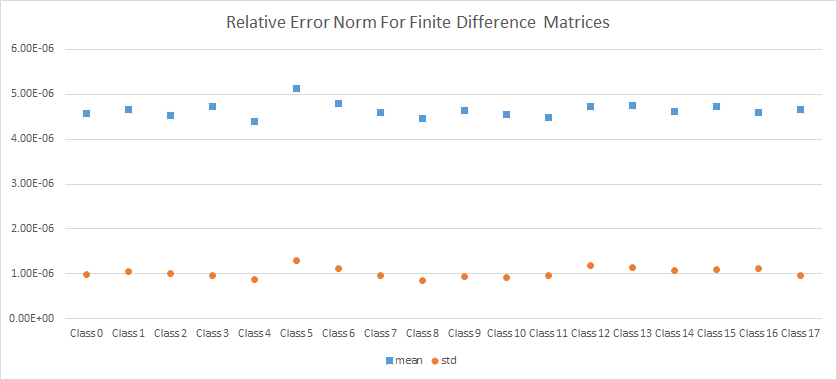
	SVD-generated Matrices		Laplacian Matrices		Finite Difference Matrices
Class No.	Mean	Std	Mean	Std	Mean	Std
Class 0	4.61e-09	4.71e-09	1.19e-07	1.86e-07	2.44e-06	2.52e-06
Class 1	4.47e-09	5.92e-09	1.04e-07	1.82e-07	2.32e-06	2.60e-06
Class 2	4.60e-09	5.82e-09	1.43e-07	2.17e-07	1.63e-06	1.79e-06
Class 3	3.47e-09	3.30e-09	7.71e-08	1.35e-07	2.07e-06	2.23e-06
Class 4	3.36e-09	3.70e-09	1.56e-07	2.64e-07	2.17e-06	2.55e-06
Class 5	4.05e-09	3.93e-09	1.34e-07	2.28e-07	1.95e-06	2.41e-06
Class 6	3.59e-09	3.32e-09	1.10e-07	1.46e-07	2.34e-06	2.47e-06
Class 7	4.21e-09	4.85e-09	1.11e-07	1.86e-07	2.28e-06	2.35e-06
Class 8	3.95e-09	3.74e-09	1.30e-07	2.18e-07	2.09e-06	2.39e-06
Class 9	3.93e-09	3.67e-09	1.19e-07	2.04e-07	2.63e-06	2.77e-06
Class 10	4.24e-09	6.16e-09	1.02e-07	1.79e-07	1.79e-06	1.77e-06
Class 11	3.77e-09	3.70e-09	1.12e-07	2.11e-07	2.31e-06	3.18e-06
Class 12	4.34e-09	4.98e-09	1.13e-07	1.83e-07	1.90e-06	2.09e-06
Class 13	5.01e-09	8.50e-09	2.32e-07	2.33e-07	5.99e-06	7.51e-06
Class 14	3.80e-09	4.37e-09	1.91e-07	2.13e-07	3.74e-06	4.49e-06
Class 15	4.30e-09	4.89e-09	1.66e-07	1.82e-07	2.64e-06	3.34e-06
Class 16	3.80e-09	4.73e-09	1.91e-07	1.95e-07	1.90e-06	2.48e-06
Class 17	3.95e-09	4.48e-09	1.81e-07	2.01e-07	2.71e-06	3.33e-06

Table 11.5: Relative Error Norms in Tests with Multipliers of Additional Classes

The outputs were quite accurate even where we applied Algorithm 5.1a with very sparse multipliers of classes 13–17.

We extended these tests of Algorithm 5.1a with additional classes of multipliers to the $n\times n$ input matrices of discretized Integral Equations from the San Jose University matrix database for $n=1000$ . The matrices came from discretization (based on Galerkin or quadrature methods) of the Fredholm Integral Equations of the first kind.

We applied our tests to the dense matrices with smaller ratios of “numerical rank/ $n$ ” from the built-in test problems in Regularization Tools,¹⁹¹⁹ 19 See http://www.math.sjsu.edu/singular/matrices and http://www2.imm.dtu.dk/ $\sim$ pch/Regutools For more details see Chapter 4 of the Regularization Tools Manual at
http://www.imm.dtu.dk/ $\sim$ pcha/Regutools/RTv4manual.pdf namely to the following six input classes from the Database:

baart: Fredholm Integral Equation of the first kind,

shaw: one-dimensional image restoration model,

gravity: 1-D gravity surveying model problem,

wing: problem with a discontinuous solution,

foxgood: severely ill-posed problem,

inverse Laplace: inverse Laplace transformation.

We summarize the results of the tests in Tables 11.6 and 11.7, where we provided the numerical rank of each input matrix in parentheses.

The results show high output accuracy with error norms in the range from about $10^{-6}$ to $10^{-9}$ with the exception of multiplier classes 13-17 for the inverse Laplace input matrix, in which case the range was from about $10^{-3}$ to $10^{-5}$ .

	wing (4)		baart (6)		inverse Laplace (25)
Class No.	Mean	Std	Mean	Std	Mean	Std
Class 0	1.20E-08	6.30E-08	1.82E-09	1.09E-08	2.72E-08	7.50E-08
Class 1	3.12E-09	1.23E-08	1.85E-09	1.71E-08	5.91E-08	2.32E-07
Class 2	1.10E-09	5.36E-09	2.01E-10	9.93E-10	4.31E-08	1.22E-07
Class 3	8.08E-09	5.77E-08	5.14E-10	3.15E-09	2.00E-08	4.95E-08
Class 4	2.62E-09	1.27E-08	2.10E-09	1.68E-08	2.13E-08	6.30E-08
Class 5	1.94E-09	9.99E-09	2.16E-09	1.91E-08	1.42E-07	5.12E-07
Class 6	2.34E-09	1.90E-08	3.81E-09	1.51E-08	2.83E-08	9.32E-08
Class 7	1.59E-09	8.88E-09	4.34E-10	2.40E-09	3.79E-08	9.40E-08
Class 8	1.78E-08	1.16E-07	1.32E-09	8.96E-09	1.65E-08	4.54E-08
Class 9	2.72E-08	2.56E-07	4.41E-10	2.11E-09	4.68E-08	1.92E-07
Class 10	4.68E-10	3.21E-09	1.12E-09	6.77E-09	3.07E-08	7.79E-08
Class 11	2.06E-09	1.40E-08	5.53E-10	2.50E-09	3.26E-08	7.80E-08
Class 12	2.19E-09	1.05E-08	3.28E-10	1.71E-09	2.35E-08	7.15E-08
Class 13	2.00E-09	1.34E-08	2.46E-09	1.40E-08	1.21E-03	4.13E-03
Class 14	7.96E-09	4.18E-08	5.31E-10	3.00E-09	6.61E-04	2.83E-03
Class 15	3.01E-09	2.23E-08	5.55E-10	2.74E-09	3.35E-04	1.81E-03
Class 16	2.27E-09	1.07E-08	2.10E-09	1.28E-08	3.83E-05	1.66E-04
Class 17	3.66E-09	1.57E-08	1.10E-09	5.58E-09	3.58E-04	2.07E-03

Table 11.6: Relative Error Norms for benchmark input matrices of discretized Integral Equations from the San Jose University singular matrix database in Tests with Multipliers of Additional Classes

	foxgood (10)		shaw (12)		gravity (25)
Class No.	Mean	Std	Mean	Std	Mean	Std
Class 0	1.56E-07	4.90E-07	2.89E-09	1.50E-08	2.12E-08	4.86E-08
Class 1	3.70E-07	2.33E-06	1.79E-08	8.70E-08	3.94E-08	1.14E-07
Class 2	2.03E-07	4.86E-07	1.99E-09	1.19E-08	1.98E-08	5.66E-08
Class 3	1.46E-07	4.06E-07	7.74E-09	4.15E-08	4.15E-08	1.15E-07
Class 4	8.45E-08	2.51E-07	7.18E-09	3.32E-08	3.22E-08	8.57E-08
Class 5	3.46E-07	1.21E-06	3.88E-09	2.11E-08	3.53E-08	9.66E-08
Class 6	1.05E-06	5.07E-06	7.11E-09	3.78E-08	3.86E-08	9.54E-08
Class 7	1.89E-07	5.36E-07	1.51E-08	5.48E-08	1.96E-08	6.43E-08
Class 8	1.30E-07	4.20E-07	7.88E-09	3.60E-08	5.12E-08	1.09E-07
Class 9	2.05E-07	5.74E-07	8.96E-09	3.45E-08	2.90E-08	7.73E-08
Class 10	1.69E-07	6.72E-07	1.07E-08	5.01E-08	2.66E-08	7.15E-08
Class 11	1.85E-07	6.20E-07	6.48E-09	3.29E-08	2.16E-08	7.46E-08
Class 12	7.60E-08	2.38E-07	9.21E-09	4.52E-08	3.98E-08	1.21E-07
Class 13	1.76E-06	3.76E-06	1.46E-08	5.92E-08	4.81E-08	1.26E-07
Class 14	9.77E-07	1.71E-06	1.11E-08	6.67E-08	2.82E-08	8.37E-08
Class 15	7.16E-07	1.14E-06	1.87E-08	1.04E-07	5.70E-08	2.52E-07
Class 16	7.52E-07	1.24E-06	4.77E-09	1.79E-08	6.32E-08	1.99E-07
Class 17	9.99E-07	2.27E-06	1.03E-08	3.81E-08	3.94E-08	1.00E-07

Table 11.7: Relative Error Norms for benchmark input matrices of discretized Integral Equations from the San Jose University singular matrix database in Tests with Multipliers of Additional Classes

11.4 Testing perturbation of leverage scores

Table 11.8 shows the means and standard deviations of the norms of the relative errors of approximation of the input matrix $W$ and of its LRA $AB$ and similar data for the maximum difference between the SVD-based leverage scores of the pairs of these matrices. We also include numerical ranks of the input matrices $W$ defined up to tolerance $10^{-6}$ .

In these tests we reused input matrices $W$ and their approximations $AB$ from our tests in Section 12.4 (using the Singular Matrix Database of San Jose University).

In addition, the last three lines of Table 11.8 show similar results for perturbed diagonally scaled factor-Gaussian matrices $GH$ with expected numerical rank $r$ approximating input matrices $W$ up to perturbations.

			LRA Rel Error		Leverage Score Error
Input Matrix	r	rank	mean	std	mean	std
baart	4	6	6.57e-04	1.17e-03	1.57e-05	5.81e-05
baart	6	6	7.25e-07	9.32e-07	5.10e-06	3.32e-05
baart	8	6	7.74e-10	2.05e-09	1.15e-06	3.70e-06
foxgood	8	10	5.48e-05	5.70e-05	7.89e-03	7.04e-03
foxgood	10	10	9.09e-06	8.45e-06	1.06e-02	6.71e-03
foxgood	12	10	1.85e-06	1.68e-06	5.60e-03	3.42e-03
gravity	23	25	3.27e-06	1.82e-06	4.02e-04	3.30e-04
gravity	25	25	8.69e-07	7.03e-07	4.49e-04	3.24e-04
gravity	27	25	2.59e-07	2.88e-07	4.64e-04	3.61e-04
laplace	23	25	2.45e-05	9.40e-05	4.85e-04	3.03e-04
laplace	25	25	3.73e-06	1.30e-05	4.47e-04	2.78e-04
laplace	27	25	1.30e-06	4.67e-06	3.57e-04	2.24e-04
shaw	10	12	6.40e-05	1.16e-04	2.80e-04	5.17e-04
shaw	12	12	1.61e-06	1.60e-06	2.10e-04	2.70e-04
shaw	14	12	4.11e-08	1.00e-07	9.24e-05	2.01e-04
wing	2	4	1.99e-02	3.25e-02	5.17e-05	2.07e-04
wing	4	4	7.75e-06	1.59e-05	7.17e-06	2.30e-05
wing	6	4	2.57e-09	1.15e-08	9.84e-06	5.52e-05
factor-Gaussian	25	25	1.61e-05	3.19e-05	4.05e-08	8.34e-08
factor-Gaussian	50	50	2.29e-05	7.56e-05	2.88e-08	6.82e-08
factor-Gaussian	75	75	4.55e-05	1.90e-04	1.97e-08	2.67e-08

Table 11.8: Tests for the perturbation of leverage scores

12 Numerical Tests of Primitive, Cynical, and Cross-Approximation (C–A) Algorithms for LRA and HSS matrices

12.1 Test Overview

We cover our tests of Primitive and C–A algorithms for CUR LRA of random input matrices and benchmark matrices of discretized Integral and Partial Differential Equations (PDEs). We have performed the tests in the Graduate Center of the City University of New York by using MATLAB. In particular we applied its standard normal distribution function ”randn()” in order to generate Gaussian matrices and calculated numerical ranks of the input matrices by using the MATLAB’s function ”rank(-,1e-6)”, which only counts singular values greater than $10^{-6}$ .

Our tables display the mean value of the spectral norm of the relative output error over 1000 runs for every class of inputs as well as the standard deviation (std).

In Section 11.3 we present the results of our tests where we incorporate C–A algorithms into the computation of low rank generators for HSS matrices.

12.2 Four algorithms used

In our tests we applied and compared the following four algorithms for computing CUR LRA to input matrices $W$ having numerical rank $r$ :

•

Tests 1 (The rtf5+ algorithm for $k=l=r$ ): Randomly choose two index sets $\mathcal{I}$ and $\mathcal{J}$ , both of cardinality $r$ , then compute a nucleus $U=W_{\mathcal{I},\mathcal{J}}^{-1}$ and define CUR LRA

$W^{\prime}:=CUR=W_{:,\mathcal{J}}\cdot W_{\mathcal{I},\mathcal{J}}^{-1}\cdot W_{\mathcal{I},\cdot}.$ (12.1)
•

Tests 2 (Five loops of C–A): Randomly choose an initial row index set $\mathcal{I}_{0}$ of cardinality $r$ , then perform five loops of C–A by applying Algorithm 1 of [P00] as a subalgorithm that produces $r\times r$ CUR generators. At the end compute a nucleus $U$ and define CUR LRA as in Tests 1.

•

Tests 3 (A Cynical algorithm for $p=q=4r$ and $k=l=r$ ): Randomly choose a row index set $\mathcal{K}$ and a column index set $\mathcal{L}$ , both of cardinality $4r$ , and then apply Algs. 1 and 2 from [P00] to compute a $r\times r$ submatrix $W_{\mathcal{I},\mathcal{J}}$ of $W_{\mathcal{K},\mathcal{L}}$ having locally maximal volume. Compute a nucleus and obtain CUR LRA by applying equation (12.1).
•

Tests 4 (Combination of a single C–A loop with Tests 3): Randomly choose a column index set $\mathcal{L}$ of cardinality $4r$ ; then perform a single C–A loop (made up of a single horizontal step and a single vertical step): First by applying Alg. 1 from [P00] find an index set $\mathcal{K}^{\prime}$ of cardinality $4r$ such that $W_{\mathcal{K}^{\prime},\mathcal{L}}$ has locally maximal volume in $W_{:,\mathcal{L}}$ , then by applying this algorithm to matrix $W_{\mathcal{K}^{\prime},:}$ find an index set $\mathcal{L}^{\prime}$ of cardinality $4r$ such that $W_{\mathcal{K}^{\prime},\mathcal{L}^{\prime}}$ has locally maximal volume in $W_{\mathcal{K}^{\prime},:}$ . Then proceed as in Tests 3 – find an $r\times r$ submatrix $W_{\mathcal{I},\mathcal{J}}$ having locally maximal volume in $W_{\mathcal{K}^{\prime},\mathcal{L}^{\prime}}$ , compute a nucleus, and define CUR LRA.

12.3 CUR LRA of random input matrices

In the tests of this subsection we computed CUR LRA with random row- and column-selection for a perturbed $n\times n$ factor-Gaussian matrices with expected rank $r$ , that is, matrices $W$ in the form

W=G_{1}*G_{2}+10^{-10}G_{3},

for three Gaussian matrices $G_{1}$ of size $n\times r$ , $G_{2}$ of size $r\times n$ , and $G_{3}$ of size $n\times n$ . Table 12.1 shows the test results for all four test algorithms for $n=256,512,1024$ and $r=8,16,32$ .

Tests 2 have output the mean values of the relative error norms in the range $[10^{-6},10^{-7}]$ ; other tests mostly in the range $[10^{-4},10^{-5}]$ .

		Tests 1		Tests 2		Tests 3		Tests 4
n	r	mean	std	mean	std	mean	std	mean	std
256	8	1.51e-05	1.40e-04	5.39e-07	5.31e-06	8.15e-06	6.11e-05	8.58e-06	1.12e-04
256	16	5.22e-05	8.49e-04	5.06e-07	1.38e-06	1.52e-05	8.86e-05	1.38e-05	7.71e-05
256	32	2.86e-05	3.03e-04	1.29e-06	1.30e-05	4.39e-05	3.22e-04	1.22e-04	9.30e-04
512	8	1.47e-05	1.36e-04	3.64e-06	8.56e-05	2.04e-05	2.77e-04	1.54e-05	7.43e-05
512	16	3.44e-05	3.96e-04	8.51e-06	1.92e-04	2.46e-05	1.29e-04	1.92e-05	7.14e-05
512	32	8.83e-05	1.41e-03	2.27e-06	1.55e-05	9.06e-05	1.06e-03	2.14e-05	3.98e-05
1024	8	3.11e-05	2.00e-04	4.21e-06	5.79e-05	3.64e-05	2.06e-04	1.49e-04	1.34e-03
1024	16	1.60e-04	3.87e-03	4.57e-06	3.55e-05	1.72e-04	3.54e-03	4.34e-05	1.11e-04
1024	32	1.72e-04	1.89e-03	3.20e-06	1.09e-05	1.78e-04	1.68e-03	1.43e-04	6.51e-04

Table 12.1: CUR LRA of random input matrices

12.4 CUR LRA of matrices of discretized Integral Equations

Table 12.2 displays the mean values of the relative error norms (mostly in the range $[10^{-6},10^{-7}]$ ) that we observed in Tests 2 applied to $1,000\times 1,000$ matrices from the Singular Matrix Database of the San Jose University. (Tests 1 produced much less accurate CUR LRA for the same input sets, and we do not display their results.) We have tested dense matrices with smaller ratios of ”numerical rank/ $\min(m,n)$ ” from the built-in test problems in Regularization Tools.²⁰²⁰ 20 See http://www.math.sjsu.edu/singular/matrices and http://www2.imm.dtu.dk/ $\sim$ pch/Regutools For more details see Chapter 4 of the Regularization Tools Manual at
http://www.imm.dtu.dk/ $\sim$ pcha/Regutools/RTv4manual.pdf The matrices came from discretization (based on Galerkin or quadrature methods) of the Fredholm Integral Equations of the first kind.

We applied our tests to the following six input classes from the Database:

baart: Fredholm Integral Equation of the first kind,

shaw: one-dimensional image restoration model,

gravity: 1-D gravity surveying model problem,

wing: problem with a discontinuous solution,

foxgood: severely ill-posed problem,

inverse Laplace: inverse Laplace transformation.

			Tests 2
Inputs	m	${\bf r}$	mean	std
baart	1000	4	1.69e-04	2.63e-06
	1000	6	1.94e-07	3.57e-09
	1000	8	2.42e-09	9.03e-10
shaw	1000	10	9.75e-06	3.12e-07
	1000	12	3.02e-07	6.84e-09
	1000	14	5.25e-09	3.02e-10
gravity	1000	23	1.32e-06	6.47e-07
	1000	25	3.35e-07	1.97e-07
	1000	27	9.08e-08	5.73e-08
wing	1000	2	9.23e-03	1.46e-04
	1000	4	1.92e-06	8.78e-09
	1000	6	8.24e-10	9.79e-11
foxgood	1000	8	2.54e-05	7.33e-06
	1000	10	7.25e-06	1.09e-06
	1000	12	1.57e-06	4.59e-07
inverse Laplace	1000	23	1.04e-06	2.85e-07
	1000	25	2.40e-07	6.88e-08
	1000	27	5.53e-08	2.00e-08

Table 12.2: CUR LRA of benchmark input matrices of discretized Integral Equations from the San Jose University Singular Matrix Database

12.5 Tests with bidiagonal pre-processing for benchmark input matrices from [HMT11]

Tables 12.3 and 12.4 display the results of Tests 1, 3, and 4 applied to pre-processed matrices of two kinds, from [HMT11, Section 7.1 and 7.2], namely, the matrices of classes (i) and (ii) from Section 11.2.

Application of Tests 1, 3, and 4 to the matrices of class (i) without pre-processing tended to produce results with large errors, and so we pre-processed every input matrix by multiplying it by 20 matrices, each obtained by means of random column permutations of a random bidiagonal matrix (see Section 8.10). Then we observed output errors in the range $[10^{-3},10^{-8}]$ , with Tests 4 showing the best performance.

In the case of the input matrices of class (ii) the results of application of Tests 1, 3, and 4 were similar with all structured and Gaussian multipliers.

		Tests 1		Tests 4
n	r	mean	std	mean	std
256	31	1.37e-04	2.43e-04	9.46e-05	2.11e-04
256	35	5.45e-05	7.11e-05	1.03e-05	1.08e-05
256	39	6.18e-06	6.32e-06	1.24e-06	1.72e-06
512	31	7.80e-05	6.00e-05	2.04e-05	1.52e-05
512	35	1.56e-04	1.53e-04	6.74e-05	1.79e-04
512	39	5.91e-05	1.10e-04	4.27e-05	1.20e-04
1024	31	9.91e-05	6.69e-05	2.79e-05	3.13e-05
1024	35	4.87e-05	4.35e-05	1.66e-05	1.50e-05
1024	39	6.11e-05	1.33e-04	3.83e-06	5.77e-06

Table 12.3: CUR LRA of Laplacian input matrices

		Tests 1		Tests 3		Tests 4
n	r	mean	std	mean	std	mean	std
800	78	4.85e-03	4.25e-03	3.30e-03	8.95e-03	3.71e-05	3.27e-05
800	82	2.67e-03	3.08e-03	4.62e-04	6.12e-04	2.23e-05	2.24e-05
800	86	2.14e-03	1.29e-03	4.13e-04	8.45e-04	6.73e-05	9.37e-05
1600	111	1.66e-01	4.71e-01	1.11e-03	1.96e-03	1.21e-04	1.17e-04
1600	115	3.75e-03	3.18e-03	1.96e-03	3.93e-03	4.03e-05	2.79e-05
1600	119	3.54e-03	2.27e-03	5.56e-04	7.65e-04	5.38e-05	8.49e-05
3200	152	1.87e-03	1.37e-03	3.23e-03	3.12e-03	1.68e-04	2.30e-04
3200	156	1.92e-03	8.61e-04	1.66e-03	1.65e-03	1.86e-04	1.17e-04
3200	160	2.43e-03	2.00e-03	1.98e-03	3.32e-03	1.35e-04	1.57e-04

Table 12.4: CUR LRA of finite difference matrices

12.6 Tests with abridged randomized Hadamard and Fourier pre-processing

Table 12.5 displays the results of our Tests 2 for CUR LRA with abridged randomized Hadamard and Fourier pre-processing. We used the same input matrices as in previous two subsections. For these input matrices Tests 1 have no longer output stable accurate LRA. For the data from discretized integral equations of Section 12.4 we observed relative error norm bounds in the range $[10^{-6},10^{-7}]$ ; for the data from Section 10 they were near $10^{-3}$ .

Multipliers				Hadamard		Fourier
Input Matrix	m	n	r	mean	std	mean	std
gravity	1000	1000	25	2.72e-07	3.95e-08	2.78e-07	4.06e-08
wing	1000	1000	4	1.22e-06	1.89e-08	1.22e-06	2.15e-08
foxgood	1000	1000	10	4.49e-06	6.04e-07	4.50e-06	5.17e-07
shaw	1000	1000	12	3.92e-07	2.88e-08	3.91e-07	2.98e-08
bart	1000	1000	6	1.49e-07	1.37e-08	1.49e-07	1.33e-08
inverse Laplace	1000	1000	25	3.62e-07	1.00e-07	3.45e-07	8.64e-08
Laplacian	256	256	15	4.08e-03	1.14e-03	3.94e-03	5.21e-04
	512	512	15	3.77e-03	1.34e-03	4.28e-03	6.07e-04
	1024	1024	15	3.97e-03	1.22e-03	4.09e-03	4.47e-04
finite difference	408	800	41	4.50e-03	1.12e-03	3.76e-03	8.36e-04
	808	1600	59	4.01e-03	1.10e-03	3.80e-03	1.70e-03
	1608	3200	80	4.60e-03	1.53e-03	3.85e-03	1.27e-03

Table 12.5: Tests 2 for CUR LRA with ARFT/ARHT pre-processors

12.7 Testing C–A acceleration of the random sampling algorithms of [DMM08]

Tables 6 and 7 display the results of our tests where we performed eight C–A iterations for the input matrices of Section 12.4 by applying Algorithm 1 of [DMM08] to all vertical and horizontal sketches (see the lines marked “C–A”), and, so overall the computations are superfast unless the C–A steps become too numerous. For comparison with this algorithm, we computed LRA of the same matrices by applying to them fast Algorithm 2 of [DMM08] (see the lines marked “CUR”). The columns of the tables marked with ”nrank” display the numerical rank of an input matrix. The columns of the tables marked with ” $k=l$ ” show the number of rows and columns in a square matrix of CUR generator. The fast algorithms have output closer approximations, but in most cases just slightly closer.

In these tests the superfast algorithm consistently yielded the same or nearly the same (within at most a factor of 10) output accuracy as the fast algorithm.

input	algorithm	m	n	nrank	k=l	mean	std
finite diff	C–A	608	1200	94	376	6.74e-05	2.16e-05
finite diff	CUR	608	1200	94	376	6.68e-05	2.27e-05
finite diff	C–A	608	1200	94	188	1.42e-02	6.03e-02
finite diff	CUR	608	1200	94	188	1.95e-03	5.07e-03
finite diff	C–A	608	1200	94	94	3.21e+01	9.86e+01
finite diff	CUR	608	1200	94	94	3.42e+00	7.50e+00
baart	C–A	1000	1000	6	24	2.17e-03	6.46e-04
baart	CUR	1000	1000	6	24	1.98e-03	5.88e-04
baart	C–A	1000	1000	6	12	2.05e-03	1.71e-03
baart	CUR	1000	1000	6	12	1.26e-03	8.31e-04
baart	C–A	1000	1000	6	6	6.69e-05	2.72e-04
baart	CUR	1000	1000	6	6	9.33e-06	1.85e-05
shaw	C–A	1000	1000	12	48	7.16e-05	5.42e-05
shaw	CUR	1000	1000	12	48	5.73e-05	2.09e-05
shaw	C–A	1000	1000	12	24	6.11e-04	7.29e-04
shaw	CUR	1000	1000	12	24	2.62e-04	3.21e-04
shaw	C–A	1000	1000	12	12	6.13e-03	3.72e-02
shaw	CUR	1000	1000	12	12	2.22e-04	3.96e-04

Table 12.6: LRA errors of Cross-Approximation (C–A) tests incorporating [DMM08, Algorithm 1] in comparison to the errors of stand-alone [DMM08, Algorithm 2] (for three input classes from Section 12.4).

input	algorithm	m	n	nrank	$k=l$	mean	std
foxgood	C–A	1000	1000	10	40	3.05e-04	2.21e-04
foxgood	CUR	1000	1000	10	40	2.39e-04	1.92e-04
foxgood	C–A	1000	1000	10	20	1.11e-02	4.28e-02
foxgood	CUR	1000	1000	10	20	1.87e-04	4.62e-04
foxgood	C–A	1000	1000	10	10	1.13e+02	1.11e+03
foxgood	CUR	1000	1000	10	10	6.07e-03	4.37e-02
wing	C–A	1000	1000	4	16	3.51e-04	7.76e-04
wing	CUR	1000	1000	4	16	2.47e-04	6.12e-04
wing	C–A	1000	1000	4	8	8.17e-04	1.82e-03
wing	CUR	1000	1000	4	8	2.43e-04	6.94e-04
wing	C–A	1000	1000	4	4	5.81e-05	1.28e-04
wing	CUR	1000	1000	4	4	1.48e-05	1.40e-05
gravity	C–A	1000	1000	25	100	1.14e-04	3.68e-05
gravity	CUR	1000	1000	25	100	1.41e-04	4.07e-05
gravity	C–A	1000	1000	25	50	7.86e-04	4.97e-03
gravity	CUR	1000	1000	25	50	2.22e-04	1.28e-04
gravity	C–A	1000	1000	25	25	4.01e+01	2.80e+02
gravity	CUR	1000	1000	25	25	4.14e-02	1.29e-01
inverse Laplace	C–A	1000	1000	25	100	4.15e-04	1.91e-03
inverse Laplace	CUR	1000	1000	25	100	5.54e-05	2.68e-05
inverse Laplace	C–A	1000	1000	25	50	3.67e-01	2.67e+00
inverse Laplace	CUR	1000	1000	25	50	2.35e-02	1.71e-01
inverse Laplace	C–A	1000	1000	25	25	7.56e+02	5.58e+03
inverse Laplace	CUR	1000	1000	25	25	1.26e+03	9.17e+03

Table 12.7: LRA errors of Cross-Approximation (C–A) tests incorporating [DMM08, Algorithm 1] in comparison to the errors of stand-alone [DMM08, Algorithm 2] (for four input classes from Section 12.4).

12.8 Computation of CUR LRAs for benchmark HSS matrices

We tested superfast computation of CUR LRA of the generators for the off-diagonal blocks of HSS matrices that approximate $1024\times 1024$ Cauchy-like matrices derived from benchmark Toeplitz matrices B, C, D, E, and F of [XXG12, Section 5]. For the computation of CUR LRA we applied the algorithm of [GOSTZ10].

Table 9.15 displays the relative errors of the approximation of the $1024\times 1024$ HSS input matrices in the spectral and Chebyshev norms averaged over 100 tests. Each approximation was obtained by means of combining the exact diagonal blocks and CUR LRA of the off-diagonal blocks (cf. Section 9). We computed CUR LRA of all these blocks superfast.

The numerical experiments covered in Table 12.8 were executed on a 64-bit Windows machine with an Intel i5 dual-core 1.70 GHz processor using software custom programmed in $C^{++}$ and compiled with LAPACK version 3.6.0 libraries.

As can be expected from our formal study, already the first C–A loop consistently yielded reasonably close CUR LRA, but our further improvement was achieved in five C–A loops in our tests for all but one of the five families of input matrices.

The reported HSS rank is the larger of the numerical ranks for the $512\times 512$ off-diagonal blocks. This HSS rank was used as an upper bound in our binary search that determined the numerical rank of each off-diagonal block for the purpose of computing its LRA. We based the binary search on minimizing the difference (in the spectral norm) between each off-diagonal block and its LRA.

The output error norms were quite low. Even in the case of the matrix C, obtained from Prolate Toeplitz matrices, known to be extremely ill-conditioned, they ranged form $10^{-3}$ to $10^{-6}$ .

We have also performed further numerical experiments on all the HSS input matrices by using a hybrid LRA algorithm: we used random pre-processing with Gaussian and Hadamard (abridged and permuted) multipliers by incorporating Algorithm 4.1 of [HMT11], but only for the off-diagonal blocks of smaller sizes while retaining our previous way for computing CUR LRA of the larger off-diagonal blocks. We have not displayed the results of these experiments because they yielded no substantial improvement in accuracy in comparison to the exclusive use of the less expensive CUR LRA on all off-diagonal blocks.

			Spectral Norm		Chebyshev Norm
Inputs	C–A loops	HSS rank	mean	std	mean	std
B	1	26	8.11e-07	1.45e-06	3.19e-07	5.23e-07
B	5	26	4.60e-08	6.43e-08	7.33e-09	1.22e-08
C	1	16	5.62e-03	8.99e-03	3.00e-03	4.37e-03
C	5	16	3.37e-05	1.78e-05	8.77e-06	1.01e-05
D	1	13	1.12e-07	8.99e-08	1.35e-07	1.47e-07
D	5	13	1.50e-07	1.82e-07	2.09e-07	2.29e-07
E	1	14	5.35e-04	6.14e-04	2.90e-04	3.51e-04
E	5	14	1.90e-05	1.04e-05	5.49e-06	4.79e-06
F	1	37	1.14e-05	4.49e-05	6.02e-06	2.16e-05
F	5	37	4.92e-07	8.19e-07	1.12e-07	2.60e-07

Table 12.8: CUR C–A approximation of HSS input matrices from [XXG12]

Appendix

Appendix A Randomized Error Estimates for LRA from [HMT11]

Halko et al. estimated the errors of Algorithm 5.1a based on the following deterministic bound on $|UV-M|$ in the case of any multiplier $H$ (they prove this bound in [HMT11, Section 10]):

|UV-M|^{2}\leq|\Sigma_{2}|^{2}+|\Sigma_{2}C_{2}C_{1}^{+}|^{2}

(A.1)

where

C_{1}=T^{*}_{1}H,~C_{2}=T^{*}_{2}H,

(A.2)

M=\begin{pmatrix}S_{1}&\Sigma_{1}&&T_{1}^{*}\\ S_{2}&&\Sigma_{2}&T_{2}^{*}\end{pmatrix},~M_{r}=S_{1}\Sigma_{1}T_{1}^{*},~{\rm and}~M-M_{r}=S_{2}\Sigma_{2}T_{2}^{*}

(A.3)

are SVDs of the matrices $M$ , its rank- $r$ truncation $M_{r}$ , and $M-M_{r}$ , respectively.

Notice that $T_{1}^{*}$ is the matrix of the top $r$ singular vectors of $M$ , $\Sigma_{2}=O$ and $UV=M$ if $\rank(M)=r$ , and the $r\times l$ matrix $C_{1}$ has full rank $r$ .

By nontrivially combining bound (A.1) with Lemma 2.1 and Theorems 4.3– 4.5, Halko et al. prove in [HMT11, Theorems 10.5 and 10.6] that

\mathbb{E}||M-UV||_{F}^{2}\leq\Big(1+\frac{r}{l-r-1}\Big)~\tau_{r+1}^{2}(M);

(A.4)

\mathbb{E}||M-UV||\leq\Big(1+\frac{r}{l-r-1}\Big)^{1/2}~\sigma_{r+1}(A)+\frac{e\sqrt{l}}{l-r}\tau_{r+1}(M),

(A.5)

in both cases provided that $2\leq r\leq l-2$ .

For $l\geq r+4$ [HMT11, Theorems 10.7 and 10.8] bound the norms $|M-UV|$ in probability as follows:

||M-UV||_{F}\leq\Big(1+t\cdot\sqrt{\frac{3r}{l-r+1}}\Big)\tau_{r+1}(M)+ut\frac{e\sqrt{l}}{l-r+1}\sigma_{r+1}(M);

(A.6)

||M-UV||\leq\Big[\Big(1+t\cdot\sqrt{\frac{3r}{l-r+1}}\Big)\sigma_{r+1}(A)+t\frac{e\sqrt{l}}{l-r+1}\tau_{r+1}(M)\Big]+ut\cdot\frac{e\sqrt{l}}{l-r+1}\sigma_{r+1}(M),

(A.7)

in both cases with a failure probability at most $2t^{r-l}+e^{-u^{2}/2}$ and in both cases Halko et al. first estimate the norms $|M-UV|$ in terms of the norms $|\Sigma_{2}|$ and $|B_{1}^{+}|$ and then invoke the assumption that $H$ is a Gaussian matrix and the estimates for the norms $|B_{1}^{+}|$ .

In the case of SRHT and SRFT multipliers [T11] and [HMT11, Theorem 11.2] prove that

|M-UV|\leq\sqrt{l+7n/l}~\tilde{\sigma}_{r+1}(M)

(A.8)

with a failure probability at most $O(1/r)$ provided that

4[\sqrt{r}+\sqrt{8\log(rn)}]^{2}\log(r)\leq l\leq n.

Appendix B Proofs of the Error Estimates for Superfast LRA

We keep writing $W_{r}$ for the rank- $r$ truncation of a matrix $W$ .

B.1 Proof of Theorems 6.2 and 6.3

Lemma B.1.

Suppose that Algorithm 5.1 has been applied to an an $m\times n$ rank- $r$ matrix $\tilde{M}$ and its perturbation $M=\tilde{M}+E$ and has output matrices $\tilde{U}$ , $\tilde{V}$ , $U$ , and $V$ , respectively, such that $\tilde{M}=\tilde{U}\tilde{V}$ . Then

M-UV=E-(W_{1}+W_{2}+W_{3}),

|M-UV|\leq|E|+|W_{1}|+|W_{2}|+|W_{3}|.

(B.1)

where

W_{1}=(U-\tilde{U})~U_{r}^{+}~M,~W_{2}=\tilde{U}~(U_{r}^{+}-\tilde{U}^{+})~M,~W_{3}=\tilde{U}~\tilde{U}^{+}~(M-\tilde{M}).

(B.2)

Furthermore

W_{1}=HEU_{r}^{+}~M,~W_{3}=\tilde{U}~\tilde{U}^{+}E,

(B.3)

|\tilde{M}H|\leq|A|\nu_{r,l}|H|~{\rm and}~|(\tilde{M}H)^{+}|\leq|H_{r}^{+}|\nu_{r,l}^{+}|A^{+}|.

(B.4)

Proof.

Substitute $M-E=\tilde{M}=\tilde{U}\tilde{V}$ , $V=U^{+}M$ , and $\tilde{V}=\tilde{U}^{+}\tilde{M}$ and obtain $M-UV-E=-(UV^{+}M-\tilde{U}\tilde{V}^{+}\tilde{M})$ . Then readily verify bounds (B.1)–(B.2). Substitute the equations $M-\tilde{M}=E$ and $U-\tilde{U}=HE$ into (B.2) and obtain (B.3). Finally deduce bounds (B.4) from Lemmas 2.1 and 2.2. ∎

Proof of Theorems 6.2. If Algorithm 5.1a is applied, then

|U|=|U^{+}|=|\tilde{U}|=|\tilde{U}^{+}|=1

and moreover

||\tilde{U}^{+}-U^{+}||\leq\sqrt{2}~||(\tilde{M}H)^{+}||~||EH||_{F}+O(||EH||_{F}^{2})

by virtue of Lemma 2.6. Thus the norm $|\tilde{U}^{+}-U^{+}|$ is in $O(|E|)$ , like $|\tilde{U}-U|$ , $|W_{1}|$ , and $|W_{3}|$ (cf. (B.3)). Now claim (i) of Theorem 6.2 readily follows from Lemma B.1; claim (ii) follows from bounds (B.4) and claim (i).

Proof of Theorem 6.3. Recall that by virtue of Corollary 2.1,

||\tilde{U}^{+}-U^{+}||\leq\frac{\mu}{1-\eta}||\tilde{U}^{+}||^{2}||\tilde{U}-U||~{\rm if}~\eta=1-||\tilde{U}^{+}||~||\tilde{U}-U||>0

(B.5)

(such a provision is assumed in Theorem 6.3) and if $\mu\leq(1+\sqrt{5})/2$ (cf. Lemma 2.5). Therefore in this case

||U^{+}||\leq||\tilde{U}^{+}||+\frac{\mu}{1-\eta}||\tilde{U}^{+}||^{2}||\tilde{U}-U||=||\tilde{U}^{+}||+O(|E|).

(B.6)

Combine the latter relationships with the equation $\tilde{U}=\tilde{M}H$ and Lemma B.1 and deduce claim (i) of Theorem 6.3. Its claim (ii) follows from claim (i) and (B.4).

B.2 Proof of Theorem 6.4

Readily deduce Theorem 6.4 by combining bound (A.1) with the following lemma.

Lemma B.2.

Under the assumptions of Theorem 6.4 let $\Sigma_{2}$ , $C_{1}$ , and $C_{2}$ denote the matrices of (A.1)–(A.3). Then (i) $|C_{2}|\leq|H|$ , (ii) $|\Sigma_{2}|\leq|E|$ , and (iii) $||C_{1}^{+}||^{-1}\geq(\nu_{{\rm sp},r,n}\nu_{{\rm sp},r,l}^{+}||H_{r}^{+}||)^{-1}-4\alpha||H||.$

Proof.

Claim (i) follows because the matrix $T_{2}^{*}$ is orthogonal, and so $|C_{2}|=|T_{2}^{*}H|\leq|T_{2}^{*}|~|H|\leq|H|$ .

Lemma 2.3 for $M=AB+E$ implies claim (ii).

It remains to estimate the norm $||C_{1}^{+}||$ . At first we do this in the special case where $E=O$ and $M=\tilde{M}=AB$ for $B\in\mathcal{G}^{r\times n}$ (cf. (6.1)); in this case we write $\tilde{C}_{1}:=C_{1}$ .

Let $A=S_{A}\Sigma_{A}T_{A}^{*}$ and $B=S_{B}\Sigma_{B}T_{B}^{*}$ be SVDs. Then

AB=S_{A}PT_{B}^{*}~{\rm for}~P=\Sigma_{A}T_{A}^{*}S_{B}\Sigma_{B},

where $P,\Sigma_{A}$ , $T_{A}^{*}$ , $S_{B}$ , and $\Sigma_{B}$ are $r\times r$ matrices. Let $P=S_{P}\Sigma_{P}T_{P}^{*}$ be SVD, write

\Sigma:=\Sigma_{P},~S:=S_{A}S_{P},~{\rm and}~T^{*}:=T_{P}^{*}T_{B}^{*},

and observe that $S$ and $T^{*}$ are orthogonal matrices of sizes $m\times r$ and $r\times n$ , respectively. Therefore $AB=S\Sigma T^{*}$ is SVD. Furthermore this is the top rank- $r$ SVD because $\rank(AB)=r$ .

Hence

\tilde{C}_{1}=T^{*}H=T_{P}^{*}T_{B}^{*}H.

Recall that $S_{B}$ and $\Sigma_{B}$ are $r\times r$ matrices and that $B\in\mathcal{G}^{r\times n}$ and deduce from SVD $B=S_{B}\Sigma_{B}T_{B}^{*}$ that $T_{B}^{*}=S_{B}^{*}\Sigma_{B}^{-1}B$ . Substitute this expression and obtain that

\tilde{C}_{1}=T_{P}^{*}S_{B}^{*}\Sigma_{B}^{-1}BH.

Notice that $T_{P}$ and $S_{B}$ are $r\times r$ orthogonal matrices, recall Lemma 2.2, and deduce that

|\tilde{C}_{1}^{+}|\leq|\Sigma_{B}|~|(BH)^{+}|.

Substitute $|\Sigma_{B}|=|B|=\nu_{r,n}$ and obtain

|\tilde{C}_{1}^{+}|\leq\nu_{r,n}|(BH)^{+}|.

Now let $H=S_{H}\Sigma_{H}T_{H}^{*}$ be SVD. Then $BS_{H}\in\mathcal{G}^{r\times l}$ by virtue of Lemma 2.1. Therefore

|(BH)^{+}|\leq\nu_{r,l}^{+}|\Sigma_{H_{r}}^{-1}|=\nu_{r,l}^{+}|H_{r}^{+}|.

Substitute this inequality into the above bound on $|\tilde{C}_{1}^{+}|$ and obtain

|\tilde{C}_{1}^{+}|\leq\nu_{r,n}\nu_{r,l}^{+}|H_{r}^{+}|.

(B.7)

Next let $M=AB+E$ where possibly $E\neq O$ , $\rank(M)>r$ , and $\tilde{C}_{1}\neq C_{1}$ , assume that

\alpha:=||E||_{F}/(\sigma_{r}(M)-\sigma_{r+1}(M))\leq 0.2

and deduce from Theorem 2.2 that there exists a unitary basis $B_{r,{\rm right}}$ of the space $\mathcal{R}(T_{M})$ of the top $r$ right singular vectors of $M$ within the Frobenius norm bound $4\alpha$ from a unitary basis for the space $\mathcal{R}(T_{AB})$ of the top $r$ right singular vectors of $M$ .

Recall that $||C_{1}^{+}||^{-1}=\sigma_{r}(C_{1})$ (cf. (2.2) and that the singular values of a matrix are invariant in its unitary transformation.

Furthermore perturbation of the matrix $T$ within the norm bound $4\alpha$ causes perturbation of $C_{1}$ within $4\alpha||H||$ and not more that that for $\sigma_{r}(C_{1})$ by virtue of Lemma 2.7. Hence

||C_{1}^{+}||^{-1}=\sigma_{r}(C_{1})\geq\sigma_{r}(\tilde{C}_{1})-4\alpha||H||=||(\tilde{C}_{1})^{+}||^{-1}-4\alpha||H||.

Substitute bound (B.7) and arrive at claim (iii) of Lemma B.2. ∎

Appendix C Computation of Sampling and Re-scaling Matrices

We begin with the following simple computations. Given an $n$ vectors ${\bf v}_{1},\dots,{\bf v}_{n}$ of dimension $l$ , write $V=({\bf v}_{i})_{i=1}^{n}$ and compute $n$ leverage scores

p_{i}={\bf v}_{i}^{T}{\bf v}_{i}/||V||^{2}_{F},i=1,\dots,n.

(C.1)

Notice that $p_{i}\geq 0$ for all $i$ and $\sum_{i=1}^{n}p_{i}=1$ .

Next assume that some leverage scores $p_{1},\dots,p_{n}$ are given to us and recall [DMM08, Algorithms 4 and 5]. For a fixed positive integer $l$ they sample either exactly $l$ columns of an input matrix $W$ (the $i$ th column with probability $p_{i}$ ) or at most $l$ its columns in expectation (the $i$ th column with probability $\min\{1,lp_{i}\}$ ), respectively.

Algorithm C.1.

[The Exactly( $l$ ) Sampling and Re-scaling.]

Input:: Two integers $l$ and $n$ such that $1\leq l\leq n$ and $n$ nonnegative scalars $p_{1},\dots,p_{n}$ such that $\sum_{i=1}^{n}p_{i}=1$ .
Initialization:: Write $S:=O_{n,l}$ and $D:=O_{l,l}$ .
Computations:: (1) For $t=1,\dots,l$ do

Pick $i_{t}\in\{1,\dots,n\}$ such that Probability $(i_{t}=i)=p_{i}$ ;

$s_{i_{t},t}:=1$ ;

$d_{t,t}=1/\sqrt{lp_{i_{t}}}$ ;

end

(2) Write $s_{i,t}=0$ for all pairs of $i$ and $t$ unless $i=i_{t}$ .
Output:: $n\times l$ sampling matrix $S=(s_{i},t)_{i,t=1}^{n,l}$ and $l\times l$ re-scaling matrix $D=\diag(d_{t,t})_{t=1}^{l}$ .

The algorithm performs $l$ searches in the set $\{1,\dots,n\}$ , $l$ multiplications, $l$ divisions, and the computation of $l$ square roots.

Algorithm C.2.

[The Expected( $l$ ) Sampling and Re-scaling.]

Input, Output and Initialization: are as in Algorithm C.1.
Computations:: Write $t:=1$ ;

for $t=1,\dots,l-1$ do

for $j=1,\dots,n$ do

Pick $j$ with probability $\min\{1,lp_{j}\}$ ;

if $j$ is picked, then

$s_{j,t}:=1$ ;

$d_{t,t}:=1/\min\{1,\sqrt{lp_{j}}\}$ ;

$t:=t+1$ ;

end

end

Algorithm C.2 involves $nl$ memory cells. $O((l+1)n)$ flops, and the computation of $l$ square roots.

Obtain the following results from [BW17, Lemmas 3.7 and 3.8] (cf. [RV07]).

Theorem C.1.

[The Impact of Sampling and Re-scaling on the Singular Values of a Matrix.]

Suppose that $n>r$ , $V\in\mathbb{C}^{n\times r}$ and $V^{T}V=I_{r}$ . Let $0<\delta\leq 1$ and $4r\ln(2r/\delta)<l$ . Define leverage scores by equations (C.1) and then compute the sampling and re-scaling matrices $S$ and $D$ by applying Algorithm C.2. Then bounds (2.5) hold with a probability at least $1-\delta$ .

Notice that $||D^{-1}||_{F}\leq\sqrt{r}$ .

Theorem C.2.

[The Impact of Sampling and Re-scaling on the Frobenius Norm of a Matrix.] Define the sampling and scaling matrices $S$ and $D$ as in Theorem C.1. Then for an $m\times n$ matrix $W$ it holds with a probability at least 0.9 that $||WSD||_{F}^{2}\leq||W||^{2}_{F}$ .

Appendix D Superfast Transition from an LRA to a CUR LRA

D.1 Superfast transition from an LRA to top SVD

Algorithm D.1.

(Superfast Transition from an LRA to the Top SVD. Cf. [HMT11, Algorithms 5.1 and 5.2].)

Input:

Four matrices $A\in\mathbb{C}^{m\times l}$ , $W\in\mathbb{C}^{l\times k}$ , $B\in\mathbb{C}^{k\times n}$ , and $M\in\mathbb{C}^{m\times n}$ such that

M=AWB+E,~||E||=O(\tilde{\sigma}_{r+1}),~r\leq\min\{k,l\},~k\ll m,~{\rm and}~l\ll n~{\rm for}~\tilde{\sigma}_{r+1}~{\rm of~Lemma~\ref{letrnc}}.

Output:

Three matrices $S\in\mathbb{C}^{m\times r}$ (unitary), $\Sigma\in\mathbb{C}^{r\times r}$ (diagonal), and $T^{*}\in\mathbb{C}^{r\times n}$ (unitary) such that $M=S\Sigma T^{*}+E^{\prime}$ for $||E^{\prime}||=O(\tilde{\sigma}_{r+1})$ .

Computations:

1.

Compute QRP rank-revealing factorization of the matrices $A$ and $B$ :

$A=(Q~|~E_{m,l-r})RP~{\rm and}~B=P^{\prime}R^{\prime}\begin{pmatrix}Q^{\prime}\\ E_{k-r,n}\end{pmatrix}$

where $Q\in\mathbb{C}^{m\times r}$ , $Q^{\prime}\in\mathbb{C}^{r\times n}$ and $||E_{m,l-r}||+||E_{k-r,n}||=O(\tilde{\sigma}_{r+1})$ . Substitute the expressions for $A$ and $B$ into the matrix equation $M=AWB+E$ and obtain $M=QUQ^{\prime}+E^{\prime}$ where $U=RPVP^{\prime}R^{\prime}\in\mathbb{C}^{r\times r}$ and $||E^{\prime}||=O(\tilde{\sigma}_{r+1})$ .
2.

Compute SVD $U=\bar{S}\Sigma\bar{T}^{*}$ . Output the $r\times r$ diagonal matrix $\Sigma$ .
3.

Compute and output the unitary matrices $S=Q\bar{S}$ and $T^{*}=\bar{T}^{*}Q^{\prime}$ .

This algorithm uses $ml+lk+kn$ memory cells and $O(ml^{2}+nk^{2})$ flops.

D.2 Superfast transition from top SVD to a CUR LRA

Given SVD of a rank- $r$ matrix $M$ , the following superfast algorithm computes CUR decomposition of $M$ .

Algorithm D.2.

[Superfast Transition from the Top SVD to a CUR LRA.]

Input:

Five integers $k$ , $l$ , $m$ , $n$ , and $r$ such that $1\leq r\leq k\leq m$ and $r\leq l\leq n$ and matrices $M\in\mathbb{C}^{m\times n}$ , $\Sigma\in\mathbb{C}^{r\times r}$ (diagonal), $S\in\mathbb{C}^{m\times r}$ , and $T\in\mathbb{C}^{n\times r}$ (both unitary) such that $1\leq r\ll\min\{m,n\}$ , $M=S\Sigma T^{*}E$ .

Output:

Three matrices $C\in\mathbb{C}^{m\times l}$ , $U\in\mathbb{C}^{l\times k}$ , and $R\in\mathbb{C}^{k\times n}$ such that $C$ and $R$ are submatrices of $M$ and

M=CUR.

Computations:

1.

By applying the algorithms of [GE96] or [P00] to the matrices $S$ and $T$ compute their $k\times r$ and $r\times l$ submatrices $S_{\mathcal{I},:}$ and $T^{*}_{:,\mathcal{J}}$ , respectively. Output the CUR factors $C=S\Sigma T^{*}_{:,\mathcal{J}}$ and $R=S_{\mathcal{I},:}\Sigma T^{*}$ .
2.

Compute and output a nucleus $U=M_{k,l,r}^{+}=M_{k,l}^{+}=T_{:,\mathcal{J}}\Sigma^{-1}S_{\mathcal{I},:}^{*}$ for the CUR generator $M_{k,l}=S_{\mathcal{I},:}\Sigma T^{*}_{:,\mathcal{J}}$ .

Correctness of the algorithm is immediately verified: $CUR=(S\Sigma T^{*}_{:,\mathcal{J}})(T_{:,\mathcal{J}}\Sigma^{-1}S_{\mathcal{I},:}^{*})(S_{\mathcal{I},:}\Sigma T^{*})=S\Sigma T^{*}$ .

The algorithm uses $kn+lm+kl$ memory cells and $O(ml^{2}+nk^{2})$ flops, and so it is superfast for $k\ll m$ and $l\ll n$ .

Let us estimate the norm $||U||$ . Clearly $||M_{k,l}||\leq||M||$ . Recall that by virtue of Theorem 2.1 $||S_{\mathcal{I},:}^{+}||\leq t_{m,l,h}$ and $||T_{:,\mathcal{J}}^{*+}||\leq t_{n,k,h}$ for $t_{q,s,h}$ of (2.4) (where we can choose, say, h=1.1) and that $||\Sigma^{-1}||=||M^{+}||=1/\sigma_{r}(M)$ . Combine these bounds with Lemma 2.2 and deduce that

||U||=||W_{k,l}^{+}||\leq||S_{\mathcal{I},:}^{+}||~||\Sigma^{-1}||~||T_{:,\mathcal{J}}^{*+}||\leq t_{m,l,h}t_{n,k,h}/\sigma_{r}(W).

(D.1)

Remark D.1.

At stage 1 we can apply the randomized algorithm of Remark 2.1, involving only $O((m+n)r+kl\min\{k,l\})$ flops, instead of the more expensive determinitic algorithms of [GE96] or [P00]. Moreover the following bound on the norm $||U||$ would replace (D.1):

||U||\leq\Big(1+\sqrt{4r\ln(2r/\delta_{1})/l}\Big)~\Big(1+\sqrt{4r\ln(2r/\delta_{2})/k}\Big)/\sigma_{r}(W)

(D.2)

with a probability at least $(1-\delta_{1})(1-\delta_{2})$ for any fixed pair of positive $\delta_{1}$ and $\delta_{2}$ not exceeding 1.

Appendix E Two Small Families of Hard Inputs for Superfast LRA

Example E.1.

Define $\delta$ -matrices of rank 1 filled with zeros except for a single entry filled with 1. There are exactly $mn$ such $m\times n$ matrices, e.g., four matrices of size $2\times 2$ :

\begin{pmatrix}1&0\\ 0&0\end{pmatrix},~\begin{pmatrix}0&1\\ 0&0\end{pmatrix},~\begin{pmatrix}0&0\\ 1&0\end{pmatrix},~\begin{pmatrix}0&0\\ 0&1\end{pmatrix}.

The output matrix of any superfast algorithm approximates nearly $50\%$ of all these matrices as poorly as the matrix filled with the vales 1/2 does. Indeed a superfast algorithm only depends on a small subset of all $mn$ input entries, and so its output is invariant in the input values at all the other entries. In contrast nearly $mn$ pairs of $\delta$ -matrices vary on these entries by 1. The approximation by a single value is off by at least 1/2 for one or both of the matrices of such a pair, that is, it is off at least as much as the approximation by the matrix filled with the values 1/2. Likewise if a superfast LRA algorithm is randomized and accesses an input entry with a probability $p$ , then with probability $1-p$ it approximates some $\delta$ -matrix with an error at least 1/2 at that entry.

Furthermore if a superfast algorithm has been applied to a perturbed $\delta$ -matrix $W$ and only accesses its nearly vanishing entries, then it would optimize LRA over the class of nearly vanishing matrices and would never detect its failure to approximate the only entry of the matrix $W$ close to 1.

Remark E.1.

$\delta$ -matrices are sparse, but subtract the rank-1 matrix filled with 1/2 from every $\delta$ -matrix and obtain a family of dense matrices of rank 2 that are not close to sparse matrices, but similarly to Example E.1, LRA of this family computed by any superfast algorithm is at best within 1/2, that is, no better than by the trivial matrix filled with zeros.

Appendix F Superfast a posteriori error estimation for LRA in a special case

In a very special but important case we obtain a posteriori error estimates simply by applying the customary basic rules of hypothesis testing for the variance of a Gaussian variable. In this case we need no upper bound on the error norm of rank- $r$ approximation.

Namely we can do this in the case where the error matrix $E$ of an LRA has enough entries, say, 100 or more, and where they are the observed i.i.d. values of a single random variable. This is realistic, for example, where the deviation of the matrix $W$ from its rank- $r$ approximation is due to the errors of measurement or rounding.

In this case the Central Limit Theorem implies that the distribution of the variable is close to Gaussian (see [EW07]). Fix a pair of integers $q$ and $s$ such that $qs$ is large enough (say, exceeds 100), but $qs=O((m+n)kl)$ and hence $qs\ll mn$ ; then apply our tests just to a random $q\times s$ submatrix of the $m\times n$ error matrix.

Under this policy we compute the error matrix at a dominated arithmetic cost in $O((m+n)kl)$ but still verify correctness with high confidence, by applying the rules of hypothesis testing for the variance of a Gaussian variable.

Let us specify this basic process for the sake of completeness. Suppose that we have observed the values $g_{1},\dots,g_{K}$ of a Gaussian random variable $g$ with a mean value $\mu$ and a variance $\sigma^{2}$ and that we have computed the observed average value and variance

\mu_{K}=\frac{1}{K}\sum_{i=1}^{K}g_{i}~{\rm and}~\sigma_{K}^{2}=\frac{1}{K}\sum_{i=1}^{K}|g_{i}-\mu_{K}|^{2},

respectively. Then, for a fixed reasonably large $K$ , both

{\rm Probability}~\{|\mu_{K}-\mu|\geq t|\mu|\}~{\rm and~Probability}\{|\sigma_{K}^{2}-\sigma^{2}|\geq t\sigma^{2}\}

converge to 0 exponentially fast as $t$ grows to the infinity (see [C46]).

Acknowledgements: Our work was supported by NSF Grants CCF–1563942 and CCF–133834 and PSC CUNY Award 69813 00 48. We are also very grateful to E. E. Tyrtyshnikov for the challenge of formally supporting empirical power of C–A iterations, to N. L. Zamarashkin for his ample comments on his work with A. Osinsky on LRA via volume maximization and on the first draft of [PLSZ17], and to S. A. Goreinov, I. V. Oseledets, A. Osinsky, E. E. Tyrtyshnikov, and N. L. Zamarashkin for valuable reprints and pointers to relevant bibliography.

References

[AMT10] H. Avron, P. Maymounkov, S. Toledo, Blendenpik: Supercharging LAPACK’s Least-squares Solver, SIAM Journal on Scientific Computing, 32, 1217–1236, 2010.
[AV06] R.I. Arriaga, S. Vempala, An Algorithmic Theory of Learning: Robust Concepts and Random Projection, Machine Learning, 63, 2, 161–182, May 2006.
[B41] A. C. Berry, The Accuracy of the Gaussian Approximation to the Sum of Independent Variates, Transactions of the American Mathematical Society, 49, 1, 122–136, 1941.
[B00] M. Bebendorf, Approximation of Boundary Element Matrices, Numer. Math., 86, 4, 565–589, 2000.
[B10] S. Börm, Efficient Numerical Methods for Non-local Operators: $\mathcal{H}^{2}$ -Matrix Compression, Algorithms and Analysis, European Math. Society, 2010.
[B11] M. Bebendorf, Adaptive Cross Approximation of Multivariate Functions, Constructive approximation, 34, 2, 149–179, 2011.
[B15] A. Björk, Numerical Methods in Matrix Computations, Springer, New York, 2015.
[BCDHKS14] G. Ballard, E. Carson, J. Demmel, M. Hoemmen, N. Knight, O. Schwartz, Communication Lower Bounds and Optimal Algorithms for Numerical Linear Algebra. Acta Numerica, 23, 1–155, 2014.
[BG65] P.A. Businger, G. H. Golub, Linear Least Squares Solutions by Householder Transformations, Numer. Math., 7, 269–276, 1965.
[BGH03] S. Börm, L. Grasedyck, W. Hackbusch, Introduction to Hierarchical Matrices with Applications, Engineering Analysis with Boundary Elements, 27, 5, 405–422, 2003.
[BGP05] A. Bini, L. Gemignani, V. Y. Pan, Fast and Stable QR Eigenvalue Algorithms for Generalized Semiseparable Matrices and Secular Equation, Numerische Mathematik, 100, 3, 373–408, 2005.
[BR03] M. Bebendorf, S. Rjasanow, Adaptive Low-Rank Approximation of Collocation Matrices, Computing, 70, 1, 1–24, 2003.
[BV88] W. Bruns, U. Vetter, Determinantal Rings, Lecture Notes in Math., 1327, Springer, 1988.
[BW14] C. Boutsidis, D. Woodruff, Optimal CUR Matrix Decompositions, ACM Symposium on Theory of Computing (STOC 2014), 353–362, ACM Press, New York, 2014. Full version in arXiv:1405.7910v2 [cs.DS] 16 July 2014.
[BW17] C. Boutsidis, D. Woodruff, Optimal CUR Matrix Decompositions, SIAM Journal on Computing, 46, 2, 543–589, 2017, DOI:10.1137/140977898.
[C46] Harald Cramér, Mathematical Methods of Statistics, Princeton University Press, 575 pages, 1999 (first edition 1946).
[C87] T. F. Chan, Rank Revealing QR-Factorizations, Linear Algebra and Its Appls., 88/89, 67–82, 1987.
[C00] B. A. Cipra, The Best of the 20th Century: Editors Name Top 10 Algorithms, SIAM News, 33, 4, 2, May 16, 2000.
[CC70] J. D. Carroll, J. J. Chang, Analysis of Individual Differences in Multidimensional Scaling via an N-Way Generalization of Eckart-Young Decomposition, Psychometrika, 35, 283–319, 1970.
[CCF04] M. Charikar, K. Chen, M. Farach-Colton, Finding Frequent Items in Data Streams, Theoretical Computer Science, 312, 1, 3–15, 2004.
[CD05] Z. Chen, J. J. Dongarra, Condition Numbers of Gaussian Random Matrices, SIAM. J. on Matrix Analysis and Applications, 27, 603–620, 2005.
[CGS07] S. Chandrasekaran, M. Gu, X. Sun, J. Xia, J. Zhu, A Superfast Algorithm for Toeplitz Systems of Linear Equations, SIAM. J. on Matrix Analysis and Applications, 29, 4, 1247–1266, 2007.
[CI94] S. Chandrasekaran, I. Ipsen, On Rank Revealing QR Factorizations, SIAM J. Matrix Anal. Appl., 15, 592–622, 1994.
[CW09] K. L. Clarkson, D. P. Woodruff, Numerical linear algebra in the streaming model, in Proc. 41st ACM Symposium on Theory of Computing (STOC 2009), pages 205–214, ACM Press, New York, 2009.
[CW13] K. L. Clarkson, D. P. Woodruff, Low Rank Approximation and Regression in Input Sparsity Time, Proceedings of the Forty-fifth Annual ACM Symposium on Theory of Computing (STOC ’13), 81–90, ACM New York, NY, USA, 2013. Full Version in arXiv:1207.6365.
[D88] J. Demmel, The Probability That a Numerical Analysis Problem Is Difficult, Math. of Computation, 50, 449–480, 1988.
[DE] Dillon Engineering, http://www.dilloneng.com/fft ip/parallel-fft.
[DK03] P. Drineas, R. Kannan, Pass Efficient Algorithms for Approximating Large Matrices, Proceedings of the 14th Annual ACM–SIAM Symposium on Discrete Algorithms (SODA 2003), pages 223–232, 2003.
[DKM06] P. Drineas, R. Kannan, M.W. Mahoney, Fast Monte Carlo Algorithms for Matrices II: Computing a Low-Rank Approximation to a Matrix, SIAM Journal on Computing, 36, 158–183, 2006.
[DMM08] P. Drineas, M.W. Mahoney, S. Muthukrishnan, Relative-error CUR Matrix Decompositions, SIAM Journal on Matrix Analysis and Applications, 30, 2, 844–881, 2008.
[DS01] K. R. Davidson, S. J. Szarek, Local Operator Theory, Random Matrices, and Banach Spaces, in Handbook on the Geometry of Banach Spaces (W. B. Johnson and J. Lindenstrauss editors), pages 317–368, North Holland, Amsterdam, 2001.
[E88] A. Edelman, Eigenvalues and Condition Numbers of Random Matrices, SIAM J. on Matrix Analysis and Applications, 9, 4, 543–560, 1988.
[E89] A. Edelman, Eigenvalues and Condition Numbers of Random Matrices, Ph.D. thesis, Massachusetts Institute of Technology, 1989.
[EGH13] Y. Eidelman, I. Gohberg, I. Haimovici, Separable Type Representations of Matrices and Fast Algorithms, volumes 1 and 2, Birkhäuser, 2013.
[ES05] A. Edelman, B. D. Sutton, Tails of Condition Number Distributions, SIAM J. on Matrix Analysis and Applications, 27, 2, 547–560, 2005.
[EW07] A. C. Elliott, W. A. Woodward, Statistical Analysis Quick Reference Guidebook: With SPSS Examples, Sage, 2007.
[FKV98/04] A. Frieze, R. Kannan, S. Vempala, Fast Monte-Carlo Algorithms for Finding Low-rank Approximations, J. of ACM, 51, 1025–1041, 2004. Proc. version in Proceedings of the 39th Annual IEEE Symposium on Foundations of Computer Science (FOCS 98), 370–378, IEEE Computer Soc. Press, 1998.
[G59] F. R. Gantmacher, Theory of Matrices, Chelsea, New York, 1959.
[G65] G. H. Golub, Numerical Methods for Solving Linear Least Squares Problem, Numerische Math., 7, 206–216, 1965.
[GE96] M. Gu, S.C. Eisenstat, An Efficient Algorithm for Computing a Strong Rank Revealing QR Factorization, SIAM J. Sci. Comput., 17, 848–869, 1996.
[GH03] L. Grasedyck, W. Hackbusch, Construction and Arithmetics of H-Matrices, Computing, 70, 4, 295–334, 2003.
[GL13] G. H. Golub, C. F. Van Loan, Matrix Computations, The Johns Hopkins University Press, Baltimore, Maryland, 2013 (fourth edition).
[GOSTZ10] S. Goreinov, I. Oseledets, D. Savostyanov, E. Tyrtyshnikov, N. Zamarashkin, How to Find a Good Submatrix, in Matrix Methods: Theory, Algorithms, Applications (dedicated to the Memory of Gene Golub, edited by V. Olshevsky and E. Tyrtyshnikov), pages 247–256, World Scientific Publishing, New Jersey, 2010. ISBN-13 978-981-283-601-4, ISBN-10-981-283-601-2.
[GT01] S. A. Goreinov, E. E. Tyrtyshnikov, The Maximal-Volume Concept in Approximation by Low Rank Matrices, Contemporary Mathematics, 208, 47–51, 2001.
[GTZ97] S. A. Goreinov, E. E. Tyrtyshnikov, N. L. Zamarashkin, A Theory of Pseudo-skeleton Approximations, Linear Algebra and Its Applications, 261, 1–21, 1997.
[H70] R. A. Harshman, Foundations of the PARAFAC Procedure: Models and Conditions for an ”Explanatory” Multi-Modal Factor Analysis, UCLA Working Papers in Phonetics, 16, 1–84, 1970.
[H02] N. J. Higham, Accuracy and Stability in Numerical Analysis, SIAM, Philadelphia, 2002.
[HMST11] N. Halko, P. G. Martinsson, Y. Shkolnisky, M. Tygert, An Algorithm for the Principal Component Analysis of Large Data Sets, SIAM J. Scientific Computation, 33, 5, 2580–2594, 2011.
[HMT11] N. Halko, P. G. Martinsson, J. A. Tropp, Finding Structure with Randomness: Probabilistic Algorithms for Constructing Approximate Matrix Decompositions, SIAM Review, 53, 2, 217–288, 2011.
[K85] D. E. Knuth, Semi-Optimal Bases for Linear Dependencies, Linear and Multilinear Algebra, 17, 1, 1–4, 1985.
[KS16] N. Kishore Kumar, J. Schneider, Literature Survey on Low Rank Approximation of Matrices, arXiv:1606.06511v1 [math.NA] 21 June 2016.
[KV16] B. N. Khoromskij, A. Veit, Efficient Computation of Highly Oscillatory Itegrals by Using QTT Tensor Approximation, Comp. Meth. Appl. Math. 16, 1, 145–159, 2016. Also available at arXiv:1408.5224, 2014.
[L07] M. Ledoux, Deviation inequalities on largest eigenvalues, Summer School on the Connections between Probability and Geometric Functional Analysis, Jerusalem, 14-19 June 2005. Geometric Aspects of Functional Analysis, Israel Seminar 2004-2005. Lecture Notes in Math. 1910, 167-219. Springer (2007) MR2349607 Zbl1130.15012
[LM00] B. Laurent, P. Massart, Adaptive Estimation of a Quadratic Functional by Model Selection, The Annals of Statistics 28, 5, 1302–1338, 2000.
Also see http://www.jstor.org/stable/2674095
[M11] M. W. Mahoney, Randomized Algorithms for Matrices and Data, Foundations and Trends in Machine Learning, NOW Publishers, 3, 2, 2011. Preprint: arXiv:1104.5557 (2011) (Abridged version in: Advances in Machine Learning and Data Mining for Astronomy, edited by M. J. Way et al., pp. 647–672, 2012.)
[MD09] M. W. Mahoney, P. Drineas, CUR Matrix Decompositions for Improved Data Analysis, Proc. Natl. Acad. Sci. USA, 106, 697–702, 2009.
[MMD08] M.W. Mahoney, M. Maggioni, P. Drineas, Tensor-CUR Decompositions for Tensor-Based Data, SIAM Journal on Matrix Analysis and Applications, 30, 3, 957–987, 2008.
[MRT05] P. G. Martinsson, V. Rokhlin, M. Tygert, A Fast Algorithm for the Inversion of General Toeplitz Matrices, Comput. Math. Appl., 50, 741–752, 2005.
[MRT06] P.-G. Martinsson, V. Rokhlin, M. Tygert. A Randomized Algorithm for the Approximation of Matrices, Applied and Computational Harmonic Analysis, 30, 1, 47–68, 2011. Also Technical Report YALEU/DCS/TR-1361, Yale University Department of Computer Science, New Haven, CT, June 2006.
[MW17] Cameron Musco, D. P. Woodruff, Sublinear Time Low-Rank Approximation of Positive Semidefinite Matrices, 58th IEEE FOCS, 672–683, 2017. DOI 10.1109/FOCS.2017.68
arXiv:1704.03371 [cs.DS], submitted to arXiv in Apr 2017, revised in Aug 2017.
[OT10] I.V. Oseledets, E.E. Tyrtyshinkov, TT-Cross Approximation for Multi- Dimensional Arrays, Linear Algebra and its Applications, 432, 70–88, 2010.
[OZ18] A.I. Osinsky, N. L. Zamarashkin, Pseudo-skeleton Approximations with Better Accuracy Estimates, Linear Algebra and Its Applications, 537, 221–249, 2018.
[P00] C.-T. Pan, On the Existence and Computation of Rank-Revealing LU Factorizations, Linear Algebra and its Applications, 316, 199–222, 2000.
[P01] V. Y. Pan, Structured Matrices and Polynomials: Unified Superfast Algorithms,
Birkhäuser/Springer, Boston/New York, 2001.
[P15] V. Y. Pan, Transformations of Matrix Structures Work Again, Linear Algebra and Its Applications, 465, 1–32, 2015.
[PLSZ16] V. Y. Pan, Q. Luan, J. Svadlenka, L.Zhao, Primitive and Cynical Low Rank Approximation, Preprocessing and Extensions, arXiv 1611.01391 (Submitted on 3 November, 2016).
[PLSZ17] V. Y. Pan, Q. Luan, J. Svadlenka, L. Zhao, Superfast Accurate Low Rank Approximation, preprint, arXiv:1710.07946 (Submitted on 22 October, 2017).
[PQY15] V. Y. Pan, G. Qian, X. Yan, Random Multipliers Numerically Stabilize Gaussian and Block Gaussian Elimination: Proofs and an Extension to Low-rank Approximation, Linear Algebra and Its Applications, 481, 202–234, 2015.
[PSZ15] V. Y. Pan, J. Svadlenka, L. Zhao, Estimating the Norms of Circulant and Toeplitz Random Matrices and Their Inverses, Linear Algebra and Its Applications, 468, 197–210, 2015.
[PW08] V. Y. Pan, X. Wang, Degeneration of Integer Matrices Modulo an Integer, Linear Algebra and Its Applications, 429, 2113–2130, 2008.
[PZ16] V. Y. Pan, L. Zhao, Low-rank Approximation of a Matrix: Novel Insights, New Progress, and Extensions, Proc. of the Eleventh International Computer Science Symposium in Russia (CSR’2016), (Alexander Kulikov and Gerhard Woeginger, editors), St. Petersburg, Russia, June 2016, Lecture Notes in Computer Science (LNCS), 9691, 352–366, Springer International Publishing, Switzerland (2016).
[PZ17a] V. Y. Pan, L. Zhao, New Studies of Randomized Augmentation and Additive Preprocessing, Linear Algebra and Its Applications, 2017. http://dx.doi.org/10.1016/j.laa.2016.09.035. Also arxiv 1412.5864.
[PZ17b] V. Y. Pan, L. Zhao, Numerically Safe Gaussian Elimination with No Pivoting, Linear Algebra and Its Applications, 527, 349–383, 2017. http://dx.doi.org/10.1016/j.laa.2017.04.007. Also arxiv 1501.05385
[RST09] V. Rokhlin, A. Szlam, M. Tygert, A Randomized Algorithm for Principal Component Analysis, SIAM Journal on Matrix Analysis and Applications, 31, 3, 1100–1124, 2009.
[RT08] V. Rokhlin, M. Tygert, A Fast Randomized Algorithm for Overdetermined Linear Least-squares Regression, Proc. Natl. Acad. Sci. USA, 105, 36, 13212–13217, 2008.
[RV07] M. Rudelson, R. Vershynin, Sampling from Large Matrices: an Approach through Geometric Functional Analysis, Journal of the ACM, 54, 4, Article number 1255449, 2007.
[RV09] M. Rudelson, R.Vershynin, Smallest Singular Value of a Random Rectangular Matrix, Comm. of Pure and Applied Mathematics, 62, 12, 1707–1739, 2009,
https://doi.org/10.1002/cpa.20294
[S95] J.-G. Sun, On Perturbation Bounds for QR Factorization, Linear Algebra and Its Applications, 215, 95–111, 1995.
[S98] G. W. Stewart, Matrix Algorithms, Vol I: Basic Decompositions, SIAM, Philadelphia, 1998.
[S06] T. Sarlós, Improved Approximation Algorithms for Large Matrices via Random Projections, Proceedings of IEEE Symposium on Foundations of Computer Science (FOCS), 143–152, 2006.
[SST06] A. Sankar, D. Spielman, S.-H. Teng, Smoothed Analysis of the Condition Numbers and Growth Factors of Matrices, SIAM J. on Matrix Analysis and Applics., 28, 2, 446–476, 2006.
[SWZ17] Z. Song, D. P. Woodruff, P. Zhong, Low Rank Approximation with Entrywise $l_{1}$ -Norm Error, Proceedings of the 49th Annual ACM Symposium on Theory of Computing (STOC 2017), 688–701, ACM Press, New York, 2017.
[T96] E.E. Tyrtyshnikov, Mosaic-Skeleton Approximations, Calcolo, 33, 1, 47–57, 1996.
[T00] E. Tyrtyshnikov, Incomplete Cross-Approximation in the Mosaic-Skeleton Method, Computing, 64, 367–380, 2000.
[T11] J. A. Tropp, Improved Analysis of the Subsampled Randomized Hadamard Transform, Adv. Adapt. Data Anal., 3, 1–2 (Special issue ”Sparse Representation of Data and Images”), 115–126, 2011. Also arXiv math.NA 1011.1595.
[TYUC17] J. A. Tropp, A. Yurtsever, M. Udell, V. Cevher, Practical Sketching Algorithms for Low-rank Matrix Approximation, SIAM J. Matrix Anal. Appl., 38, 4, 1454–1485, 2017. Also see arXiv:1609.00048 January 2018.
[TZ12] M. Thorup, Y. Zhang, Tabulation-based 5-independent Hashing with Applications to Linear Probing and Second Moment Estimation, SIAM J. on Computing, 41, 2, 293–331, 2012.
[VVGM05] R. Vandebril, M. Van Barel, G. Golub, N. Mastronardi, A Bibliography on Semiseparable Matrices, Calcolo, 42, 3–4, 249–270, 2005.
[VVM07/08] R. Vandebril, M. Van Barel, N. Mastronardi, Matrix Computations and Semiseparable Matrices (Volumes 1 and 2), The Johns Hopkins University Press, Baltimore, Maryland, 2007.
[VVVF10] M. Van Barel, R. Vandebril, P. Van Dooren, K. Frederix, Implicit Double Shift $QR$ -algorithm for Companion Matrices, Numerische Mathematik, 116, 177–212, 2010.
[W14] D.P. Woodruff, Sketching As a Tool for Numerical Linear Algebra, Foundations and Trends in Theoretical Computer Science, 10, 1–2, 1–157, 2014.
[WZ13] S. Wang, Z. Zhang, Improving CUR Matrix Decomposition and the Nyström Approximation via Adaptive Sampling, Journal of Machine Learning Research, 14, 1, 2729–2769, 2013.
[X12] J. Xia, On the Complexity of Some Hierarchical Structured Matrix Algorithms, SIAM J. Matrix Anal. Appl., 33, 388–410, 2012.
[X13] J. Xia, Randomized Sparse Direct Solvers, SIAM J. Matrix Anal. Appl., 34, 197–227, 2013.
[XXCB14] J. Xia, Y. Xi, S. Cauley, V. Balakrishnan, Superfast and Stable Structured Solvers for Toeplitz Least Squares via Randomized Sampling, SIAM J. Matrix Anal. Appl., 35, 44–72, 2014.
[XXG12] J. Xia, Y. Xi, M. Gu, A Superfast Structured Solver for Toeplitz Linear Systems via Randomized Sampling, SIAM J. Matrix Anal. Appl., 33, 837–858, 2012.
[YGL18] W. Yu, Y. Gu, Y. Li, Efficient Randomized Algorithms for the Fixed-Precision Low-Rank Matrix Approximation, arXiv:1606.09402. February 2018.