Computing The Analytic Connectivity of A Uniform Hypergraph
Abstract
The analytic connectivity, proposed as a substitute of the algebraic connectivity in the setting of hypergraphs, is an important quantity in spectral hypergraph theory. The definition of the analytic connectivity for a uniform hypergraph involves a series of polynomial optimization problems (POPs) associated with the Laplacian tensor of the hypergraph with nonnegativity constraints and a sphere constraint, which poses difficulties in computation. To reduce the involved computation, properties on the algebraic connectivity are further exploited, and several important structured uniform hypergraphs are shown to attain their analytic connectivities at vertices of the minimum degrees, hence admit a relatively less computation by solving a small number of POPs. To efficiently solve each involved POP, we propose a feasible trust region algorithm (FTR) by exploiting their special structures. The global convergence of FTR to the second-order necessary conditions points is established, and numerical results for both small and large size examples with comparison to other existing algorithms for POPs are reported to demonstrate the efficiency of our proposed algorithm.
Key words. Uniform hypergraph; Laplacian tensor; Analytic connectivity; Feasible trust region algorithm
AMS subject classifications. 05C65, 15A18, 90C55
1 Introductions
Spectral graph theory is a well-studied and highly applicable subject, which focuses on the connection between properties of a graph and the eigenvalues of matrices associated with the graph. Such matrices include the adjacency matrix, the Laplacian matrix and the signless Lpalacian matrix of the graph [3, 10, 15, 16, 39]. However, the study of graphs cannot fully meet the developments of modern science and technology, especially in big data analysis and complex networks. This motivates the study of hypergraphs, where an edge may connect more than two vertices [1, 2], comparing to two-vertices edges in ordinary graphs. Spectral hypergraph theory correspondingly emerged which was based upon matrix spectral analysis in its early stage.
In 2005, Lim [41] and Qi [49] independently introduced the concept of eigenvalues for tensors, which initiated the study of tensor spectral theory and paved a way for the development of spectral hypergraph theory via tensors. The related research include spectral hypergraph theory [12, 13, 23, 35, 36, 38, 45, 47, 53, 54, 59, 65], eigenvalues [29, 37, 46, 55, 56, 57, 58, 61, 63], connectivity [28, 40], Laplacian tensor [5, 30, 32, 48, 50, 64], structured tensors related [9, 14], special hypergraphs [6, 31, 34, 51, 62], hypergraph properties [7, 20, 22, 42, 43]. The tensors studied in these papers include adjacency tensors, Laplacian tensors and signless Laplacian tensors of hypergraphs. Benefitting from the high sparsity of these tensors, Chang, Chen and Qi [8] recently proposed a CEST algorithms for computing extremal eigenvalues of large-scale adjacency tensors, Laplacian tensors and signless Laplacian tensors of uniform hypergraphs, which provides a useful computational tool for spectral hypergraph theory via tensors.
It is well-known that in spectral graph theory, the algebraic connectivity [19], defined as the second smallest eigenvalue of the Laplacian matrix of a graph, is an important quantity. However, as Laplacian tensors of uniform hypergraphs may have complex eigenvalues, a different approach for generalizing this concept to hypergraphs was introduced by Qi in [50], where the analytic connectivity for a uniform hypergraph was defined via an optimization formulation
This is shown to be linked with the edge connectivity of the hypergraph. It was further studied by Li, Cooper and Chang in [40] where the analytic connectivity was shown to be connected with other important invariants of hypergraphs, such as the degree, the vertex connectivity, the diameter and the isoperimetric number.
To our best knowledge, no efficient algorithm has been proposed for computing the analytic connectivity of a uniform hypergraph in the literature. The definition of analytic connectivity involves a series of polynomial optimization problems. For dimension large enough, this is very costly. To fix this issue, we firstly explore some specific hypergraphs, and shown some properties on the vertices the analytic connectivity will possibly attained.
For each specific , we propose a feasible trust region algorithm for the computation of this quantity. Note that the analytic connectivity involves a series of optimization problems, each of which possesses nonnegativity constraints and a sphere constraint. Thus, they are special cases of the following general constrained optimization problem
| (1.1) |
where is a nonconvex polynomial function and is a nonlinear smooth function. Existing optimization algorithms for (1.1) can be roughly classified into three types. The first type includes the penalty methods, which incorporates the equality constrains into the objective function as a penalty term, and attempt to solve (1.1) by a sequential minimization problems of the form
where the objective function could be any penalty function such that the subproblem can be easily solved. For instance, the L-BFGS method [4], the gradient projection method [17, 18], and the active set method [26], etc. The solver MINOS belongs to this type. However, as the hard constraint has been relaxed as a penalty term in the objective, this type of methods usually result in an infeasible point for our sphere constraint. The second type of methods involves solving
where the objective function is always with some interior-point penalty of the nonnegativity constraint and the solver IPOPT belongs to this type. With the equality constraint in the above subproblem, this type of methods is always time consuming. The third type includes the sequential quadratic programming methods, which solves the subproblem
where the objective function is a quadratic function using the information of the Lagrangian function or its variants [21]. This type of methods show their strength when the constraints have significant nonlinearity, and the solver SNOPT belongs to this type.
Note that the constraint in this paper is actually the -norm sphere constraint. By exploring this special structure, we propose a feasible trust region method (FTR), the mixture of trust region method and the projection method, in which the projection step ensures the feasibility of each iteration and the trust region technique enhances the convergence. FTR was also used in [27] for computing Z-eigenvalues of symmetric tensors. While the main difference is that here we adopted the -norm trust region instead of the Euclidean norm, which remarkably facilitates the computation as at each iteration only a linear constrained quadratic subproblem needs to be handled. Infinity norm was also used in [24] for bound constrained problems, where advantages in terms of computational costs were demonstrated.
This paper is organized as follows. In Section 2, several related basic concepts and properties on hypergraphs and the analytic connectivity are reviewed. Further properties on the vertices attainable for the analytic connectivity is discussed in Section 3 to reduce the computation by cutting down the number of the involved POPs. For each POP, an FTR algorithm for computing the analytic connectivity of a uniform hypergraph is proposed in Section 4. The global convergence to the second order stationary points is established in Section 5. Numerical results are reported in Section 6, which demonstrates the efficiency of our proposed algorithm, and indicates that the analytic connectivity is a good choice to characterize the connectivity of the involved hypergraph as well. Conclusions are drawn in Section 7.
Notations throughout the paper are listed here. Let and be any two positive integers. We use to denote the space of all -th order -dimensional tensors. is used to stand for the set of all nonnegative vectors in . For any and any integer , denotes the -th component of , with any given positive integer , and is the diagonal matrix generated by . For any set , denotes the cardinality of . The index set is simply denoted as . The notation denotes the combinatorial number of choosing from .
2 Preliminaries
As a natural extension of a graph, a hypergraph with the vertex set and the edge set allows each of its edge joins any number of vertices. If each edge connects exactly vertices, this hypergraph is called a -uniform hypergraph, or simply called as a -graph. For more details on hypergraphs, refer to [1, 2, 12]. Obviously, is reduced to an ordinary graph when . Thus, we assume throughout the paper.
Many important structured hypergraphs have been introduced in the literature. Let be a uniform hypergraph. is called a sunflower if there is a disjoint partition of the vertex set as such that and , and ([31]); is called a hypercycle if there are subsets , , of the vertex set such that , and for the other cases, the intersections , , are mutually different, and ([32]); is called a squid if we can number the vertex set as such that the edge set , , , ([31]); More generally, is called a -path of length if and . Particularly, we call a -path hypergraph as a loose path; is called a complete -graph if .
Some related fundamental concepts of uniform hypergraphs are reviewed as follows.
Definition 2.1 ([12, 50]).
Let be a -graph. The adjacency tensor of is defined as the -th order -dimensional tensor whose -entry is:
Let be a -th order -dimensional diagonal tensor with its diagonal element being , the degree of vertex , for all . is called the degree tensor corresponding to . Then Laplacian tensor of is defined as , and the signless Laplacian tensor of as .
Definition 2.2 ([50]).
Let be a -graph with vertices. The analytic connectivity of is defined as
| (2.1) |
where
| (2.2) |
with the Laplacian tensor of .
Let be a -graph with vertices. For each vertex , denote by the set of edges containing the vertex , i.e., . The degree of the vertex is the cardinality of the set . Denote by , and the maximum, minimum and average degree of , respectively. Existing results on analytic connectivity of a uniform hypergraph include the following:
- •
[50] ; if and only if is connected;
- •
[50] , where is the edge connectivity of , defined as the minimum cardinality of an edge cut of ;
- •
[50] ;
- •
[40] , where is the complete -graph;
- •
[40] denote as the vertex connectivity of , defined as the minimum cardinality of a vertex cut of ,
(2.3) - •
[40] where is the isoperimetric number, or the Cheeger constant of , defined by , and is an edge cut of ;
- •
[40] , where diam is the diameter of , defined as the maximum distance between any pair of vertices of ;
- •
[40]
It is worth pointing out that the isoperimetric number or the Cheeger constant of an ordinary graph provides a numerical measure of whether or not a graph has a “bottleneck”, which has wide applications such as in constructing well-connected networks of computers and card shuffling. However, the computation of such an invariant is very difficult and the algebraic connectivity provides a reasonable good bound in terms of the well-known “Cheeger inequality” in the ordinary graph case. This result is in a certain sense theoretically extended to the uniform hypergraphs as stated above by Li, Cooper and Chang [40] where the analytical connectivity was adopted instead of the algebraic connectivity. In this regard, the computational algorithm presented in this paper makes the theoretical result of [40] practically feasible to efficiently bound the isoperimetric number of a -graph.
3 Properties on the analytic connectivity
In this section, we will discuss the properties on finding which vertices of a uniform hypergraph the analytic connectivity will possibly be attained at. This will henceforth play an essential role in reducing the required computation for the analytic connectivity by cutting down the number of POPs involved in Definition 2.2. We begin with the following important lemma.
Lemma 3.1.
Let be a -graph with , and be any two vertices with edge sets and . If , then , where and are defined as in (2.2).
Proof: Let and , where and are the degrees of vertices and , respectively. For any , denote as the Laplacian function corresponding to any given edge . For any satisfying , we have
For any satisfying , we have
Note that the vertex is only contained in the edges of and hence only exists in the first term of the right hand side of the above expression. To achieve the minimum value in (2.2), it is evident from the nonnegativity constraint that for any optimal solution of the problem (2.2) with , it holds that . Therefore, is also a feasible solution of the problem (2.2) with . This immediately shows the desired inequality. Q.E.D.
With the help of Lemma 3.1, we can show that for several important uniform hypergraphs, such as sunflowers, hypercycles, squids and loose path, the computation of their analytic connectivities can be significantly reduced by the following theorem.
Theorem 3.2.
Let be a -graph with the vertex set . If is a sunflower, or a hypercycle, or a squid, or a loose path, then , where is a vertex with the minimum degree.
Proof: Let be a -graph with . (i) If is a sunflower, then we can find a disjoint partition of the vertex set , says , such that and , and , where . Let . Obviously, has degree and other vertices all have degree . Moreover, for any , . Invoking of Lemma 3.1, the desired result follows readily in this case. (ii) If is a hypercycle, then there exist subsets , , of the vertex set such that , and for the other cases. From the definition of hypercycles, we know that each intersected vertex has degree two and others has degree one. And for any of degree two, there exists a vertex such that . Thus, by applying Lemma 3.1, the desired result is obtained in this case. (iii) If is a squid, then we can number the vertex set as such that the edge set , , , . Note that the vertices all have degree two and others all have degree one, and for every vertex with degree two, there exist vertex such that . Thus, from Lemma 3.1, we have . (iv) Similar to case (ii), we can prove the case when is a loose path by definition and Lemma 3.1. This completes the proof. Q.E.D.
Two more specific uniform hypergraphs are discussed whose analytic connectivities can be computed via solving (2.2) with special choices of . The first one is the -path with vertices which is plotted as follows.

Proposition 3.3.
Let be a -path -graph with vertices, defined as in Figure 3.1. Then , where could be any element in . Moreover, is monotonically decreasing with .
Proof: First we consider the first part of the proposition. It is trivial when . For , the desired result can be obtained immediately from the symmetric structure of and Lemma 3.1. Before proceeding for general cases of , we will introduce the following useful function for any given even integer ,
It is easy to see that from the homogeneous structure of the above minimization problem. Moreover, we claim that is decreasing with . Let , be any two even integers satisfying . For any optimal solution of problem with dimension , is a feasible solution of dimension . Hence
where the first equality comes from the fact that the formulation of is the same with . Furthermore, for any even integer , is negative. This comes from the claim above and the observation that given , .
For any even integer , it holds that Suppose that for some , , then the index set can be partitioned into , , and . Hence can be rewritten as
| (3.1) |
where , , and . Note that the variable in (3.1) are partitioned into three subvectors, thus
It follows from t is negative that , and the objective function is reduced to , as decreasing with , hence
where . Hence By direct computation we have and . When , it holds that ; otherwise, . Thus,
| (3.2) |
As is monotonically decreasing with , so is the analytic connectivity from (3.2). This completes the proof. Q.E.D.
The second specific one, termed as , is the -graph obtained by deleting an arbitrary edge from a complete -graph . For example, when , , the edge set of are , , , as shown in Figure 3.2.

Proposition 3.4.
Suppose is the hypergraph generated by deleting an edge from . Then , where is some vertex in , i.e.,
| (3.3) |
Proof: Without loss of generality, suppose that the edge is deleted. By the symmetric property of this hypergraph, to show (3.3), we only need to prove . For satisfying and , we have
If ,
| (3.4) |
otherwise,
| (3.5) |
For the case , it holds that . It follows from (3.4) that
where the last inequality follows from the arithmetic-geometric mean inequality that for all . In fact, the lower bound can be achieved by set as
Hence,
As discussed above, those vertices of the smallest degree are highly possible to help attain the analytic connectivity of a uniform hypergraph. A conjecture comes as follows.
Conjecture 3.1 Let be a -graph. for some of the smallest degree.
4 A feasible trust region algorithm
In this section, we propose the feasible trust region method (FTR) for solving (2.1). Noting that the projection to the -norm sphere and nonnegative space are easy. Hence, we manage to project the iterate points to the feasible set, while maintaining the convergence.
The problem (2.2) can be rewritten as follows
| s.t. | ||||
| (4.1) |
which is equivalent to
| s.t. | ||||
| (4.2) |
where is the subtensor of indexed by .
Before describing the details of FTR algorithm, the following functions are given. The Lagrangian function of (4.2) is
| (4.3) |
and its gradient vector and Hessian matrix are
| (4.4) | ||||
| (4.5) |
where , , , . Here, is a vector with the -th element being
and with the -th element denoted as
The function vector is the subvetcor of , indexed by , and the matrix is submatrix of .
4.1 The feasible trust region algorithm
Given the current point , the trust region subproblem of (4.2) can be reformulated as follows,
| s.t. | ||||
| (4.6) |
where , , , is the trust region radius updated in (4.11).
In order to facilitate the computation of (4.6), we utilize the following strategies. Firstly, we adopt the -norm in (4.6), and hence all the constrains will be linear. Secondly, at each iteration, the feasibility of implies that , which ensures the feasibility of the resulting trust region subproblem. Consequently, each subproblem is formulated as
| s.t. | ||||
| (4.7) |
Specifically, at each iteration, if the trial step is accepted, the iterate is projected to be feasible by setting , where
| (4.8) |
is a projection operator to the -norm sphere and is the -norm of . Set
| (4.9) |
which is actually the Lagrange multiplier as will be clarified in (5.2).
The following definitions are commonly used in trust region methods. Denote the ratio of actual decrease and predicted decrease as
| (4.10) |
This is an important value for evaluating the error between and at . If is large enough, we are confident to increase the trust region radius ; but if is less than a threshold, we have to decrease the radius. Specifically, is updated as follows
| (4.11) |
where are constants with and . We only update in the next iteration when is greater than or equal to some threshold,
| (4.12) |
where is a constant. It should be noted that when updated, is defined as the projection instead of .
The detailed descriptions of the FTR method for computing the analytic connectivity (2.1) of symmetric tensors is as follows. The algorithm includes two steps: the outer step and the inner step. In the outer step, given an index , let , and compute . In the inner step, the problem (4.7) is solved by the feasible trust region algorithm to compute .
- Step 0.
-
Given an initial point , set the parameters , , . Let , =0.
- Step 1.
- Step 2.
-
Let . Output and .
It is worth pointing out that if the involved uniform hypergraph has some special structure, such as those discussed in Section 3, then the computation in Algorithm 1 can be significantly reduced since the number of the outer loop can be cut down by merely considering those of the minimum degree.
5 Convergence analysis
The first-order and the second-order optimality conditions of (4.2) are stated, and the global convergence of Algorithm 1 is established in this section.
5.1 Optimality conditions
For any local minimizer of (4.2), the fact implies that the set is linearly independent, where is the identity vector with the -th element being one while the other elements are zero, and is the active set of . Thus, the linear independence constraint qualification (LICQ) holds automatically. This observation immediately leads to the following first-order and second-order necessary conditions for (4.2) by invoking Theorems 12.1 and 12.5 in [44].
Lemma 5.1.
(First-order necessary conditions) Suppose that is a local solution of (4.2). Then there is a Lagrange multiplier such that
| (5.1) |
where . Further, we have
| (5.2) |
5.2 Global convergence
In this subsection, we establish the global convergence of the inner problem of Algorithm 1; i.e., using feasible trust region algorithm to solve the problem (4.2). We shall employ the techniques in traditional trust region methods to derive the results. However, there are two key difficulties. Firstly, is updated by instead of in order to keep the feasibility. We should estimate the error between with its second order approximation, instead of . Secondly, -norm is applied, hence the outline of proof is different from Euclidean-norm cases.
To simplify our analysis, define
Then the gradient and the Hessian of are
| (5.5) |
where . A key property is that when and , we have
| (5.6) |
and
| (5.7) |
That is, the feasible direction satisfying , the second order approximations of and are the same. Several technical lemmas are presented for the convergence analysis.
Lemma 5.3.
Proof. They are obvious since , and are smooth and bounded on the closed sets. Q.E.D.
Lemma 5.4.
Proof. By the mean value theorem for integration, we have
for some . It follows from , (5.6) and (5.7) that
To show the above inequality by Lemma 5.3 (), we still need to prove and are positive. The feasible point satisfies . As two norms are equivalent, i.e., for if , then
Hence, it follows from that for , . Furthermore, it follows from , and that . Therefore,
As a result, both and are lower bounded. Q.E.D.
Lemma 5.5.
Proof. Suppose the theorem is false, we assume that
| (5.14) |
If (5.14) fails, there exists a const , such that for infinite many , it holds that
| (5.15) |
Denote the set of satisfying (5.15) as . Without loss of generality, suppose
According to our assumption, is not a stationary point of (4.2), hence is not the optimal solution of the following system
| s.t. | ||||
| (5.16) |
Denote as its solution, then
It follows from Lemma 5.6 that
for all large enough. As a result, for all large enough . This contradicts to . The contradiction indicates that (5.14) holds.
If (5.14) holds, there exists a subsequence such that
| (5.17) |
Without loss of generality, suppose
| (5.18) |
According to our assumption, is not a stationary point of (4.2), hence is not the optimal solution of the following system
| s.t. | ||||
| (5.19) |
Denote as its solution, then
As is the solution of (5.19) with the trust region radius replaced by . Then . It follows from Lemma 5.6 that
| (5.20) |
for all large enough, where the last inequality comes from . Further,
| (5.21) |
This, together with (5.20), derives , which contradicts with (5.17). This completes the proof. Q.E.D.
Lemma 5.6.
Proof. As satisfies , there exists at least an index such that . For two points and near , there exists a positive value such that
where the last inequality follows from that is bounded, and is continuous. If and or and , then is a feasible solution for
| s. t. | ||||
| (5.23) |
Otherwise, suppose that , from that there exists some positive index such that and , hence is a feasible solution for the above problem. Therefore, from the fact that the objective function of (5.23) is continuous and that is only a feasible solution, we have
On the other hand, we can show . Therefore, (5.22) holds true. Q.E.D.
Theorem 5.7.
Proof. We show this theorem by contradiction. Suppose that there exists a negative eigenvalue satisfying
| (5.24) |
It follows from the definition of (5.4) that is a feasible solution of (4.7) with replaced by , and replaced by 1. For all , either or , and for all , , hence
| (5.25) |
When is close enough to , it follows from the proof of Lemma 5.6 and that is a feasible point for the problem (4.7), where is small enough to be bounded by . Furthermore, it follows from (5.25) that is small, . Hence is an decrease direction for the problem (4.7). Therefore,
Since , , then and
| (5.26) |
It follows from (5.21) that . Therefore, there exists large enough such that
| (5.27) |
which derives that . This contradicts with . Thus, (5.24) is false. Q.E.D.
6 Numerical experiments
In this section, we present several numerical results of computing the analytic connectivity. Our codes are implemented in MATLAB (R2014a). All the experiments are preformed on a Dell desktop with Intel dual core i7-4770 CPU at 3.40 GHz and 8GB of memory running Windows 7. The parameters are set as
We execute the FTR algorithm 100 times with different initial points, and report the average results. The initial points are generated by the following Matlab commands
for rd = 1:100; randn(’seed’, rd); x0 = randn(n-1,1); end;
which obey the Gaussian distribution. Afterwards, is restricted to the feasible set of (4.2) by doing the projection .
FTR is compared with an Sparse Nonlinear OPTimizer solver SNOPT [52], which is called by the free trial software TOMLAB 11 1 http://tomopt.com/tomlab/. The exact gradient and the Hessian are provided for FTR and SNOPT, and both the quadratic programming subproblems of FTR and SNOPT are computed by SQOPT. Furthermore, for small dimensional problems, we utilize the global optimization software GloptiPoly 3 [33] 22 2 http://homepages.laas.fr/henrion/software/gloptipoly/ to solve (4.2), which can help us to judge whether our solution is the global optimal solution. GloptiPoly 3 relaxes the polynomial problem into a hierarchy of semidefinite subproblems, which are solved by SDPNAL+ [60].
Noting that the main computation of FTR includes calculating , and . To deal with this, we adopt the methods in Chang, Chen and Qi [8] to calculate , , where they store a uniform hypergraph by a compact matrix , where is the number of edges, and is the number of vertices in an edge; namely, the -th edges of the hypergraph is the -th row of as
The computational method for follows the same strategy. Thus, the computation cost for , , are , and , respectively. It should also be noted that the sparsity ratio of is
Thus our method enjoys fast computation when the sparsity property is utilized.
6.1 Comparison of FTR with SNOPT and GloptiPoly 3 for small size hypergraphs
In this subsection, we show the numerical results of our FTR algorithm, compared with SNOPT and GloptiPoly 3. We will use the hypergraphs in Figure 6.1 which are found in [8, 31, 32, 50] as the testing instances.

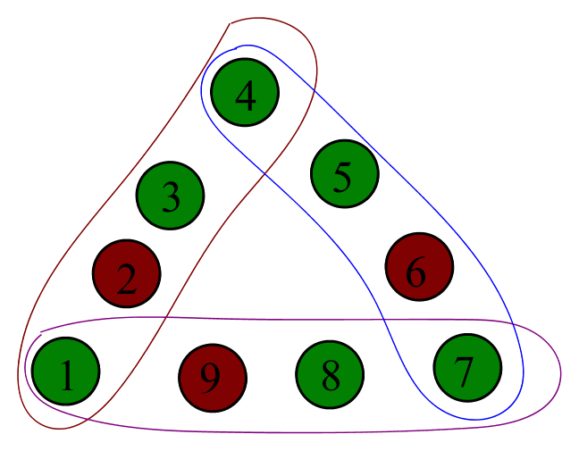


In Table 6.1, ‘’ is the number of edges of the hypergraph, ‘’ is the number of vertices, is the number of vertices in an edge. ‘’ means the analytic connectivity returned by FTR and SNOPT, ‘’ stands for the analytic connectivity computed from the global optimization software GloptiPoly 3, ‘ratio’ means the ratio FTR and SNOPT get the same result with GloptiPoly 3, and ‘iter’ is the average number of iterations of 100 runs with random initializations. ‘time (s)’ denotes the average CPU time of seconds consumed by FTR and SNOPT, or the total CPU time of GloptiPoly 3.
| SNOPT | FTR | GloptiPoly 3 | |||||||||
|---|---|---|---|---|---|---|---|---|---|---|---|
| Hypergraph | () | ratio | iter | time (s) | ratio | iter | time (s) | time (s) | |||
| (a) | (3, 8, 4) | 0.2516 | 100% | 323.61 | 0.3065 | 0.2516 | 100% | 75.42 | 0.0332 | 0.2516 | 59.515 |
| (b) | (3, 9, 4) | 0.2100 | 100% | 403.64 | 0.3619 | 0.2100 | 100% | 83.65 | 0.0365 | 0.2100 | 110.14 |
| (c) | (3, 7, 3) | 0.1607 | 100% | 142.15 | 0.1007 | 0.1607 | 97% | 48.15 | 0.0185 | 0.1607 | 74.136 |
| (d) | (8, 8, 3) | 0.4300 | 100% | 151.46 | 0.1216 | 0.4300 | 100% | 67.03 | 0.0263 | 0.4300 | 110.10 |
| (e) | (2, 4, 3) | 0.5344 | 100% | 42.28 | 0.0381 | 0.5344 | 100% | 25.28 | 0.0080 | 0.5344 | 23.052 |
| (f) | (4, 13, 4) | 0.0592 | 100% | 850.18 | 0.8496 | 0.0592 | 97% | 131.77 | 0.0603 | 0.0592 | 18.877 |
Table 6.1 shows that both SNOPT and FTR produce the same results with GloptiPoly3 for almost 100%. This is in accord with Theorem 5.7 that FTR converges to second order necessary points, which has a high possibility to converge to global optimal point. Besides, the average iteration number that FTR takes is relatively small comparing to that of SNOPT, since FTR has utilized the trust region technique. As the main computation costs in each iteration for both FTR and SNOPT are to solve the quadratic programming, this makes FTR take less CPU time than SNOPT, as one can see from Table 6.1. Additionally, it is known from Table 6.1 that, among the above six hypergraph instances, the hypergraph (f) has the smallest analytic connectivity, while (d) and (e) have relatively large ones. This, to some extent, reflects the connectivity of the corresponding hypergraphs as can be seen from Figure 6.1.
6.2 Larger dimensional problems
In this subsection, we are ready to compute relatively large dimensional problems by FTR, and compare its performance with that of SNOPT. As GloptiPoly 3 will be too costly both in time and in space for large problems, we will not consider this algorithm here. Similar to the small dimensional cases, we also give 100 initial points, and show the overall and average results. We take the -path -graph as discussed in Proposition 3.3 and in Proposition 3.4 for testing instances with different values of . The computational results are shown in Tables 6.2 and 6.3, where ‘’ is the analytic connectivity in question, and ‘ratio’ stands for the percentage from 100 experiments to achieve that minimal value.
| FTR | SNOPT | |||||||
|---|---|---|---|---|---|---|---|---|
| ratio | iter | time (s) | ratio | iter | time (s) | |||
| 10 | 1.21e-01 | 100% | 11.67 | 0.0058 | 1.21e-01 | 100% | 48.66 | 0.0408 |
| 50 | 4.11e-03 | 92% | 12.46 | 0.0095 | 4.11e-03 | 95% | 186.16 | 0.1426 |
| 100 | 1.01e-03 | 82% | 15.00 | 0.0233 | 1.01e-03 | 86% | 268.11 | 0.2554 |
| 200 | 2.49e-04 | 98% | 14.92 | 0.0872 | 2.49e-04 | 79% | 534.81 | 1.3374 |
| 300 | 1.10e-04 | 95% | 14.86 | 0.2274 | 1.10e-04 | 73% | 816.92 | 4.6972 |
| 400 | 6.20e-05 | 96% | 14.50 | 0.4935 | 6.20e-05 | 87% | 1039.38 | 11.7781 |
| 500 | 3.96e-05 | 94% | 14.71 | 0.9096 | 3.96e-05 | 89% | 1329.87 | 26.4040 |
We can see from Table 6.2 that both FTR and SNOPT produce the same optimal value for each of the above instances, and the successful ratio is above 70%, while FTR is slightly better than SNOPT. Comparing to those small size problems as computed in Subsection 6.1, large dimensional problems here are relatively hard to achieve the global optimum with local optimal algorithms such as FTR and SNOPT. For the iteration number, we find that FTR scales well for dimension as large as 500, while SNOPT takes far more iteration steps for larger dimensional problems. This leads to overwhelming superiority of FTR in computation time comparing to SNOPT, as one can see from Table 6.2. Besides, it is worth pointing out that the sparse ratio of the Hessian matrix for this problem is about , and both the quadratic subproblems of FTR and SNOPT have taken this advantage. Thus, the overall computation time is not long even when the iteration number as big as more than 1000. Additionally, we can see that as increases, is monotonically decreasing, which fits the result in Proposition 3.3.
The numerical results for with and different values of are shown in Table 6.3, with the comparison on performances of FTR and SNOPT, and the upper bounds given in (2.3). As already known from Proposition 3.4, . Combining with the inherited symmetric structure of , we only need to compute .
| FTR | SNOPT | upper bound | |||||||
|---|---|---|---|---|---|---|---|---|---|
| ratio | iter | time (s) | ratio | iter | time (s) | ||||
| 10 | 7.7736 | 100% | 6.82 | 0.0031 | 7.7736 | 100% | 30.01 | 0.0262 | 7.7778 |
| 20 | 17.8943 | 100% | 7.27 | 0.0072 | 17.8943 | 100% | 17.56 | 0.0226 | 17.8947 |
| 30 | 27.9309 | 100% | 8.03 | 0.0242 | 27.9309 | 100% | 14.48 | 0.0455 | 27.9310 |
| 40 | 37.9487 | 100% | 8.67 | 0.0764 | 37.9487 | 100% | 13.29 | 0.1578 | 37.9487 |
| 50 | 47.9592 | 100% | 8.54 | 0.2082 | 47.9592 | 100% | 14.72 | 0.5159 | 47.9592 |
| 60 | 57.9661 | 100% | 8.38 | 0.4900 | 57.9661 | 100% | 15.18 | 1.8829 | 57.9661 |
| 70 | 67.9710 | 100% | 8.01 | 1.6986 | 67.9710 | 100% | 15.85 | 7.1758 | 67.9710 |
| 80 | 77.9747 | 100% | 8.00 | 3.2806 | 77.9747 | 100% | 14.80 | 20.4195 | 77.9747 |
| 90 | 87.9775 | 100% | 8.01 | 6.1458 | 87.9775 | 100% | 15.09 | 45.8924 | 87.9775 |
| 100 | 97.9798 | 100% | 8.00 | 13.7736 | 97.9798 | 100% | 15.42 | 89.7867 | 97.9798 |
From Table 6.3, we can see that FTR takes less iterations and hence less CPU time than that of SNOPT, and the upper bound given in (2.3) is quite tight as it is pretty close to the value from computation. In addition, as the hypergraph is well connected by definition, the analytic connectivity is relatively high comparing to all the others in this section, which again verify that the analytic connectivity is a good choice to measure the connectivity of hypergraphs. However, as one can see from Tables 6.2 and 6.3, big analytic connectivities of hypergraphs result in more CPU time for the corresponding hypergraphs with the same .
7 Conclusions
In this paper, we have exploited properties on the analytic connectivity and have shown that several structured uniform hypergraphs attain their analytic connectivities at vertices of the minimum degrees. To efficiently compute the analytic connectivity of any general uniform hypergraph, we have proposed a feasible trust region algorithm with global convergence, and have conducted numerical experiments to shown the advantages of our algorithm in comparison of other existing ones. All the numerical results have verified that the analytic connectivity is a good choice to measure the connectivity of a hypergraph. Moreover, the efficiency of the proposed algorithm makes the extended version of “Cheeger inequality” in the setting of uniform hypergraphs practically feasible to efficient bound the Cheeger numbers of uniform hypergraphs.
Acknowledgements
The first author thank Professor Wei Li and Miss Lizhu Sun for their useful discussions on Conjecture 3.1. The first, third and forth authors were supported in part by the Research Grants Council (RGC) of Hong Kong (Project C1007-15G), the second author’s work was supported by the National Natural Science Foundation of China (11301022,11431002), and the third author’s work was supported by Grants No. PolyU 501212, 501913, 15302114 and 15300715.
References
- [1] C. Berge, Hypergraphs, Combinatorics of Finite Sets, 3rd edn., North-Holland, 1989.
- [2] A. Bretto, Hypergraph Theory: An Introduction, Springer, 2013.
- [3] A.E. Brouwer and W.H. Haemers, Spectra of Graphs, Springer, 2011.
- [4] R. H. Byrd, P. Lu, J. Nocedal, et al. “A limited memory algorithm for bound constrained optimization”, SIAM Journal on Scientific Computing 16(5) (1995) 1990-1208.
- [5] C. Bu, Y. Fan and J. Zhou, “Laplacian and signless Laplacian Z-eigenvalues of uniform hypergraphs”, Frontiers of Mathematics in China (2015) 1-10.
- [6] C. Bu, J. Zhou and Y. Wei, “E-cospectral hypergraphs and some hypergraphs determined by their spectra”, Linear Algebra and Its Applications 459 (2014) 397-403.
- [7] S.R. Bulò and M. Pelillo, “New bounds on the clique number of graphs based on spectral hypergraph theory”, International Conference on Learning and Intelligent Optimization, Springer Verlag, Berlin (2009) 45-58.
- [8] J. Chang, Y. Chen and L. Qi, “Computing eigenvalues of large scale sparse tensors arising from a hypergraph”, to appear in: SIAM Journal on Scientific Computing (2016).
- [9] Z. Chen and L. Qi, “Circulant tensors with applications to spectral hypergraph theory and stochastic process”, Journal of Industrial and Management Optimization 12 (2016) 1227-1247.
- [10] F.R.K. Chung, Spectral Graph Theory, American Mathematical Society, 1997.
- [11] A.R. Conn, N.M. Gould and P.L. Toint, “A globally convergent augmented Lagrangian algorithm for optimization with general constraints and simple bounds”, SIAM Journal on Numericl Analysis 28 (1991) 545-572.
- [12] J. Cooper and A. Dutle, “Spectra of uniform hypergraphs”, Linear Algebra and Its Applications 436 (2012) 3268-3292.
- [13] J. Cooper and A. Dutle, “Computing hypermatrix spectra with the Poisson product formula”, Linear and Multilinear Algebra 63 (2015) 956-970.
- [14] R. Cui, W. Li and M. Ng, “Primitive tensors and directed hypergraphs”, Linear Algebra and Its Applications 471 (2015) 96-108.
- [15] D.M. Cvetković, M. Doob, I. Gutman and A. Torgas̈ev, Recent Results in the Theory of Graph Spectra, North Holland, Amsterdam, 1988.
- [16] D.M. Cvetković, M. Doob and H. Sachs, Spectra of Graphs, Theory and Application, Academic Press, 1980.
- [17] P. H. Calamai, J. J. Moré, “Projected gradient methods for linearly constrained problems”, Mathematical Programming 39 (1987) 93-116.
- [18] Y. Dai , R. Fletcher, “New algorithms for singly linearly constrained quadratic programs subject to lower and upper bounds”, Mathematical Programming 106 (2006) 403-421.
- [19] M. Fiedler, “Algebraic connectivity of graphs”, Czechoslovak mathematical journal 23 (1973) 298-305.
- [20] Y. Fan, Y. Tan, X. Peng and A. Liu, “Maximizing spectral radii of uniform hypergraphs with few edges”, to appear in: Discussiones Mathematicae Graph Theory (2016).
- [21] M. P. Friedlander and M. A. Saunders, “A globally convergent linearly constrained lagrangian method for nonlinear optimization”, SIAM Journal on Optimization 15 (2005) 863-897.
- [22] D. Ghoshdastidar and A. Dukkipati, “Consistency of spectral partitioning of uniform hypergraphs under planted partition model”, Advances in Neural Information Processing Systems (2014) 397-405.
- [23] D. Ghoshdastidar and A. Dukkipati, “A Provable Generalized Tensor Spectral Method for Uniform Hypergraph Partitioning”, Proceedings of the 32nd International Conference on Machine Learning, Lille, France (2015) 400-409.
- [24] S. Gratton, M. Mouffe, P. L. Toint and M. Weber-Mendonca, “ A recursive-trust-region method for bound-constrained nonlinear optimization”, IMA Journal of Numerical Analysis 28(4) (2008), 827-861.
- [25] W. Hager, B. Mair and H. Zhang, “An affine-scaling interior-point CBB method for box-constrained optimization”, Mathematical Programming 119 (2009) 1-32.
- [26] W. Hager and H. Zhang, “A New Active Set Algorithm for Box Constrained Optimization”, SIAM Journal on Optimization 17 (2006) 526-557.
- [27] C. Hao, C. Cui and Y. Dai, “A feasible trust region method for calculating extreme Z-eigenvalues of symmetric tensors”, Pacific Journal of Optimization 11 (2015) 291-307.
- [28] S. Hu and L. Qi, “Algebraic connectivity of an even uniform hypergraph”, Journal of Combinatorial Optimization 24 (2012) 564-579.
- [29] S. Hu and L. Qi, “The eigenvectors associated with the zero eigenvalues of the Laplacian and signless Laplacian tensors of a uniform hypergraph”, Discrete Applied Mathematics 169 (2014) 140-151.
- [30] S. Hu and L. Qi, “The Laplacian of a uniform hypergraph”, Journal of Combinatorial Optimization 29 (2015) 331-366.
- [31] S. Hu, L. Qi and J. Shao, “Cored hypergraphs, power hypergraphs and their Laplacian eigenvalues”, Linear Algebra and Its Applications 439 (2013) 2980-2998.
- [32] S. Hu, L. Qi and J. Xie, “The largest Laplacian and signless Laplacian H-eigenvalues of a uniform hypergraph”, Linear Algebra and Its Applications 469 (2015) 1-27.
- [33] D. Henrion, J. Lasserre and J. Löfberg, “GloptiPoly 3: moments, optimization and semidefinite programming”, Optimization Methods & Software 24 (2009) 761-779.
- [34] L. Kang, V. Nikiforov and X. Yuan, “The -spectral radius of -partite and -chromatic uniform hypergraphs”, Linear Algebra and Its Applications 478 (2015) 81-107.
- [35] M. Khan and Y. Fan, “On the spectral radius of a class of non-odd-bipartite even uniform hypergraphs”, Linear Algebra and Its Applications 480 (2015) 93-106.
- [36] M. Khan, Y. Fan and Y. Tan, “The H-spectra of a class of generalized power hypergraphs”, Discrete Mathematics 339 (2016) 1682-1689.
- [37] G. Li, L. Qi and G. Yu, “The Z-eigenvalues of a symmetric tensor and its application to spectral hypergraph theory”, Numerical Linear Algebra with Applications 20 (2013) 1001-1029.
- [38] H. Li, J. Shao and L. Qi, “The extremal spectral radii of -uniform supertrees”, Journal of Combinatorial Optimization 32 (2016) 741-764.
- [39] X.L. Li, Y.T. Shi and I. Gutman, Graph Energy, Springer, 2012.
- [40] W. Li, J. Cooper and A. Chang, “Analytic connectivity of -uniform hypergraphs”, Linear and Multilinear Algebra, doi/abs/10.1080/03081087.2016.1234575 (2016).
- [41] L-H. Lim, “Singular values and eigenvalues of tensors: A variational approach”, Proceedings of the 1st IEEE International Workshop on Computational Advances in Multi-Sensor Adaptive Processing (CAMSAP), December 13-15 (2005) 129-132.
- [42] V. Nikiforov, “Analytic methods for uniform hypergraphs”, Linear Algebra and Its Applications 457 (2014) 455-535.
- [43] V. Nikiforov, “Some extremal problems for hereditary properties of graphs”, The Electronic Journal of Combinatorics 21 (2014) 1-17.
- [44] J. Nocedal and S. Wright, Numerical optimization, Springer Science & Business Media, 2006.
- [45] K. Pearson, “Spectral hypergraph theory of the adjacency hypermatrix and matroids”, Linear Algebra and Its Applications 465 (2015) 176-187.
- [46] K. Pearson and T. Zhang, “Eigenvalues on the adjacency tensor of products of hypergraphs”, International Journal on Contemporary Mathematical Sciences 8 (2013) 151-158.
- [47] K. Pearson and T. Zhang, “On spectral hypergraph theory of the adjacency tensor”, Graphs and Combinatorics 30 (2014) 1233-1248.
- [48] K. Pearson and T. Zhang, “The Laplacian tensor of a multi-hypergraph”, Discrete Mathematics 338 (2015) 972-982.
- [49] L. Qi, “Eigenvalues of a real supersymmetric tensor”, Journal of Symbolic Computation 40 (2005) 1302-1324,
- [50] L. Qi, “-Eigenvalues of Laplacian and signless Lapaclian tensors”, Communications in Mathematical Sciences 12 (2014) 1045-1064.
- [51] L. Qi, J. Shao and Q. Wang, “Regular uniform hypergraphs, -cycles, -paths and their largest Laplacian H-eigenvalues”, Linear Algebra and Its Applications 443 (2014) 215-227.
- [52] P. E. Gill, M. Walter, and M. A. Saunders. “SNOPT: An SQP algorithm for large-scale constrained optimization”, SIAM review 47 (2005) 99-131.
- [53] J. Shao, L. Qi and S. Hu, “Some new trace formulas of tensors with applications in spectral hypergraph theory”, Linear and Multilinear Algebra 63 (2015) 971-992.
- [54] J. Shao, H. Shan and B. Wu, “Some spectral properties and characterizations of connected odd-bipartite uniform hypergraphs”, Linear and Multilinear Algebra 63 (2015) 2359-2372.
- [55] J. Xie and A. Chang, “On the Z-eigenvalues of the signless Laplacian tensor for an even uniform hypergraph”, Numerical Linear Algebra with Applications 20 (2013) 1030-1045.
- [56] J. Xie and A. Chang, “On the Z-eigenvalues of the adjacency tensors for uniform hypergraphs”, Linear Algebra and Its Applications 430 (2013) 2195-2204.
- [57] J. Xie and A. Chang, “H-eigenvalues of the signless Laplacian tensor for an even uniform hypergraph”, Frontiers of Mathematics in China 8 (2013) 107-128.
- [58] J. Xie and L. Qi, “The clique and coclique numbers’ bounds based on the H-eigenvalues of uniform hypergraphs”, International Journal of Numerical Analysis & Modeling 12 (2015) 318-327.
- [59] J. Xie and L. Qi, “Spectral directed hypergraph theoy via tensors”, Linear and Multilinear Algebra 64 (2016) 780-794.
- [60] L. Yang, D. Sun and K. Toh, “SDPNAL+: a majorized semismooth Newton-CG augmented Lagrangian method for semidefinite programming with nonnegative constraints”, Mathematical Programming Computation 7 (2015) 331-366.
- [61] X. Yuan, L. Qi and J. Shao, “The proof of a conjecture on largest Laplacian and signless Laplacian H-eigenvalues of uniform hypergraphs”, Linear Algebra and Its Applications 490 (2016) 18-30.
- [62] X. Yuan, J. Shao and H. Shan, “Ordering of some uniform supertrees with larger spectral radii”, Linear Algebra and Its Applications 495 (2016) 206-222.
- [63] X. Yuan, M. Zhang and M. Lu, “Some upper bounds on the eigenvalues of uniform hypergraphs”, Linear Algebra and Its Applications 484 (2015) 540-549.
- [64] J. Yue, L. Zhang and M. Lu, “The largest adjacency, signless Laplacian, and Laplacian H-eigenvalues of loose paths”, Frontiers of Mathematics in China (2016) 1-23.
- [65] J. Zhou, L. Sun, W. Wang and C. Bu, “Some spectral properties of uniform hypergraphs”, The Electronic Journal of Combinatorics 21 (2014) 4-24.