Dynamical Space-Time and Gravitational Waves
Abstract
According to General Relativity gravity is the result of the interaction between matter and space-time geometry. In this interaction space-time geometry itself is dynamical: it can store and transport energy and momentum in the form of gravitational waves. We give an introductory account of this phenomenon and discuss how the observation of gravitational waves may open up a fundamentally new window on the universe.
1 Gravity
One hundred years ago Albert Einstein published his first papers on a new theory of gravitational interactions: General Relativity (GR) [1, 2] . It is a marvelous achievement as it connected two hitherto completely separate braches of mathematics in one physical framework: field theory and geometry. It is such a rich theory that even hundred years later we have not yet worked out all aspects of it. Moreover in spite of many creative ideas and numerous efforts the question how it fits together with quantum theory has yet to find a completely convincing and satisfying answer.
The connection between geometry and the physics of gravity can be approached from both sides.
The physical approach is to start from elementary observations about free fall. Such observations
suggest two principles underlying the nature of gravity:
a. Universality: all bodies are subject to gravity independent of their nature and composition.
b. Equivalence principle: all other circumstances being equal bodies of different mass fall with
the same gravitational acceleration.
The equivalenc principle was established in the 16th century by an experiment with lead balls
dropped from the tower of the New Church of Delft in the Netherlands by the flemish engineer and
mathematician Simon Stevin and his dutch friend Johan de Groot. Stevin published a description of
this experiment in his widely read book Principles of the art of weighing [3].
Both principles were embodied by Newton in his theory of gravity. Newton’s law states that the gravitational force between two bodies depends only on their masses and and the relative distance , and is proportional to the product of the masses
whilst the acceleration of any one of the bodies, say that of mass , is the ratio of the force and its mass
Thus the acceleration depends on the mass of the other body which can be considered the source of the gravitational force experienced by , but not on that of the body falling toward itself.
A weakness of Newton’s theory, recognized by Newton himself, was that it required instantaneous action at a distance. Two centuries later it was replaced by Einstein’s theory of General Relativity, which also incorporates the universality and equivalence principle but attributes them to the geometry of the space-time in which bodies are moving, not to some force acting instantaneously over arbitrary large distances. This theory is build around the concept of a dynamical space-time, the properties of which are determined by the masses and motion of the objects it contains. At the same time these motions are constrained by the geometry of the space-time, making space-time itself the medium through which gravitational interactions between bodies take place.
2 Field Theory
Field theory was developed in the 19th century, mainly in connection with understanding the phenomena of electricity and magnetism. Based on the work by such people as Ampère, Oersted and Faraday eventually Maxwell came up with a unified theory of electric and magnetic phenomena created by charges and currents, in which the idea of fields permeating all of space was essential. The appearance of a charge at some point in space created a local change in the field which propagated to other places at large but finite speed, eventually influencing the motion of other charges. Maxwell’s theory does not require instantaneous action at a distance, as all interactions between charges and fields are local. Moreover Maxwell’s theory has another feature which was only understood after great effort, mostly by the work of Lorentz: it incorporates special relativity as it is invariant under rotations and Lorentz transformations. Once Einstein recognized this to be a universal feature of physical phenomena it then motivated Minkowski to introduce the concept of unified space-time as a framework for physics, rather than separate newtonian space and time.
It may strike the reader that there exist close similarities between this description of fields mediating electro-magnetic interactions and the decription of space-time geometry mediating gravitational interactions. There is indeed a field-theoretic approach to General Relativity that allows the reconstruction of GR starting from the theory of a symmetric tensor field [4]. However, having the full theory of General Relativity at our disposal, it is easier and more convenient to reverse the procedure and derive the linear theory of a symmetric tensor field as a limit of GR for small-curvature perturbations in a Minkowski space-time. According to this procedure gravity can be described in the limit of weak fields in a flat space-time by a Lorentz-covariant tensor field subject to the following inhomogenous linear field equation11 1 Unless stated otherwise we use natural units in which .:
| (1) |
Here is a symmetric tensor representing the source of the field and is a coupling constant defining the strength of the interaction between the field and the source . For consistency the divergence of the tensor has to vanish:
| (2) |
This is an important point to be addressed in detail in the following. First we turn to General Relativity and the Einstein equations, and show how to obtain and interpret eq. (1) as its Minkowski limit.
3 General Relativity
According to General Relativity gravity is an effect of space-time geometry. The mathematical ingredients of this geometry are the metric, the connection and the curvature. We briefly introduce these concepts here with the additonal aim to introduce our notation; more details can be found in the literature [5, 6].
The metric is the tool which allows us to convert co-ordinate measurements into physical space and time intervals. In particular a proper-time interval measured in a local rest frame can be expressed in terms of a quadratic form of co-ordinate intervals:
| (3) |
Proper time is used to parametrize time-like curves , in particular the world-lines of massive particles. The unit tangent vector of the world-line is the 4-velocity:
| (4) |
As usual the overdot denotes an ordinary proper-time derivative. The inverse of the metric is used very often as well, and is distinguished by using superscripts for its components:
| (5) |
The connection is a quantity defining geodesics, the world-lines of particles in free fall. On such world-lines the 4-velocity only changes by parallel transport:
| (6) |
Here is the Riemann-Christoffel connection and is called the covariant derivative along the world-line. The covariant derivative and the connection are defined in such a way that the metic itself is covariantly constant:
| (7) |
which implies that we can identify the connection with a linear combination of gradients of the metric:
| (8) |
Because of this property it is clear that in free fall (on time-like geodesics) the metric changes only by parallel transport as well:
| (9) |
Finally the curvature measures the relative acceleration of geodesics; it is encoded in the Riemann tensor
| (10) |
Suppose we have two particles on world lines and ; see fig. 1. For small separation can be replaced by the tangent vector of the geodesic cutting the two world-lines in points of equal proper time . The second derivative of this vector w.r.t. proper time then represents the proper acceleration between the particles on the two world-lines.
t]
Again defining its covariant derivative by parallel transport:
by some straightforward algebra it can be established that up to quadratic corrections satisfies the condition
| (11) |
Thus the components of the Riemann tensor at some point in space-time can be measured by determining the proper acceleration between various geodesics passing through that point. Obviously if the curvature vanishes there will be no relative acceleration, and the world-lines are straight as expected in flat space.
From the Riemann tensor one can construct the Ricci tensor and the Riemann scalar by contraction:
| (12) |
Like the metric, the Ricci tensor is symmetric. Therefore the Einstein equations can fix the local geometry of space-time by relating the Ricci tensor directly to the energy-momentum distributions of matter and radiation as described by the symmetric energy-momentum tensor :
| (13) |
where the constant of proportionality is related to Newtons constant of gravity:
| (14) |
Equation (13) provides 10 independent inhomogeneous partial differential equations for the 10 independent components of the metric.
The simplest solution of the Einstein equations in empty space is Minkowski space-time. It has a constant metric which can be taken in the form
| (15) |
corresponding to pseudo-euclidean co-ordinates in which the proper-time element reads
| (16) |
As mentioned above this space-time has no curvature: the Riemann tensor vanishes, and geodesics are straight lines.
Next we consider geometries with non-vanishing but small curvature. The metric of such a space-time will be close to the Minkowski metric (13) and we expand it as
| (17) |
As the metric itself is dimensionless, the constant is introduced to give the canonical dimensions of a tensor field in 4-dimensional space-time. We can now compute the connection and the Ricci tensor under the assumption . This guarantees that the geometry does not deviate strongly from Minkowski space-time. Therefore in calculating other geometrical quantities we may restrict ourselves to expressions linear in ; in this limit the connection becomes
| (18) |
where the switch from upper- to lower-index vectors and tensors has been made using the Minkowski metric. Similarly the Ricci tensor and the Riemann scalar take the form
| (19) |
Here the box operator represents the usual d’alembertian in Minkoswki space-time:
| (20) |
From this result it follows that the Einstein equations expanded to first order in reduce to equation (1). Thus we see that this linear field equation for the symmetric tensor field describes the fluctuations of space-time geometry close to flat Minkowski geometry.
4 Gravitational Waves
An important property of eq. (1) for the symmetric tensor field is its invariance under local gauge transformations
| (21) |
From the geometrical point of view of General Relativity these gauge transformations represent the reduction of general co-ordinate transformations to the theory of small fluctutations of Minkowski geometry. From the point of view of tensor field theory in Minkowski space-time the gauge invariance guarantees that the 10 components of the field actually describe only two propagating physical modes and that as a consequence a number of components of are redundant. Let us see in more detail how this works.
First we are going to simplify the field equation by considering its trace; this results in
| (22) |
Therefore we can rewrite the tensor field equation in the form
| (23) |
As we have only rewritten the equation by grouping the elements differently the equation is still invariant under the gauge transformations (21). We now use this freedom to impose additional conditions on the tensor field. For example, we can perform a gauge transformation with parameters which are solutions of the equation
| (24) |
Then the transformed field satisfies both the field equation (23) and in addition the gauge condition
| (25) |
Moreover the field equation (23) then simplifies further to
| (26) |
In particular in empty space the equation reduces to the massless wave equation
| (27) |
showing that the free tensor field describes gravitational waves propagating with the speed of light in Minkowski space-time.
Next we recall a mathematical theorem stating that Poincaré invariance (invariance under translations and Lorentz transformations) in 4-dimensional space-time implies that massless waves of vector and tensor fields possess only 2 transverse polarisation modes. This is actually well-known in the case of electro-magnetic waves, as the electric and magnetic fields are always directed at right angles to the direction of propagation. Here we derive the corresponding result for the symmetric tensor field. In brief the argument uses the observation that eq. (24) specifies the gauge parameters only up to solutions of the homogeneous equation
| (28) |
Gauge transformations of this type can be used to eliminate still more components of the field. For example, one can eliminate the trace with the result that also the 4-dimensional divergence of the field vanishes:
| (29) |
The full analysis is most conveniently done in momentum space. Thus we expand the field in plane waves
| (30) |
where the reality of requires . Then eqs. (25) and (27) are replaced by
| (31) |
whilst the residual gauge transformations (21), (28) imply freedom to make redefinitions
| (32) |
provided the momenta take values on the light-cone . Now clearly also eq. (31) allows non-zero solutions for only if the momenta are on the light-cone. Therefore we can write
| (33) |
such that
| (34) |
Substitution of this expression for in the plane-wave expansion (30) allows us to perform the integral over the time component , with the result
| (35) |
The two terms arise from the two solutions for in eq. (34). In the second term we can now replace the integration variable and use the complex conjugation condition on in eq. (33) to finally get
| (36) |
In addition the gauge condition (31) for the amplitude implies after splitting space- and time-components and the replacement :
| (37) |
Here and in the following we extend the summation convention for repeated indices to apply also for 3-dimensional space-like indices .
Recall that the residual gauge transformations (32) are also defined on the light-cone . On the amplitudes they act as
| (38) |
If we make the following choice for the gauge parameters:
| (39) |
it is straightforward to show with the help of the first equation (37) that
| (40) |
By the second equation (37) it follows in addition that
| (41) |
In summary, starting from the field equation we can by mere gauge transformations restrict the plane-wave solutions for the tensor field to the light-cone and make them purely spatial, traceless and transverse. For example if the 3-momentum points in the -direction: , the amplitude can be decomposed as
| (42) |
where represent the individual mode-amplitudes contributing to the Fourier integral and the polarisation tensors are of the form
| (43) |


These polarization modes can be easily visualized. The -mode defines a change in the metric components and of opposite sign. Hence when physical distances in the -direction increase, those in the -direction decrease by the same amount, and vice versa. The -mode changes the distances at 45∘ to the - and -axes in a similar way. If one imagines a ring of test masses in a plane perpendicular to the direction of the wave, this ring will deformed by the two polarization modes of a wave as sketched in figure 2.
5 Energy considerations
With the gauge choice (25) the original wave equation (1) reduces to
| (44) |
This equation can actually be derived from a hamiltonian as we now show. This hamiltonian is an expression in the fields and conjugate momenta :
| (45) |
The standard Hamilton equations of motion read
| (46) |
Using the expression (45) this gives:
| (47) |
Combining these equations one gets back eq. (44). Now consider some volume in space; the integral (45) restricted to this volume at a fixed time may be considered as the total energy of the field in that volume. Its variation in time is
| (48) |
Here is the boundary surface of the volume , is a surface element of the boundary and is the normal component of the gradient to that surface element. The physical interpretation of this equation is, that the energy inside the volume changes only by a flux of gravitational radiation through the boundary, up to changes in the material energy-momentum density inside. In particular for stationary sources the energy can only change by radiation flowing through the surface .
The energy flux itself is given by
| (49) |
This establishes a quantitative relation between energy flux and amplitude of gravitational waves. For example, if we take a plane wave in the -direction like in eq. (42), (43) they generate a dimensionless metric fluctuation
| (50) |
and the energy flux in the -direction per unit of area is
| (51) |
where we have restored the the factors of so we can express the quantities in SI units. For example an energy flux of mW/m2 for a single polarisation mode at a frequency Hz corresponds to an amplitude
| (52) |
From this example one can learn two things:
(i) The amplitude of metric deformations by gravitational waves are extremely small; the metric
deformation for the wave in our example implies that the distance between the mirrors of an interferometer
with an arm length of 1 km changes by 1/100th of the diameter of a proton.
(ii) Space is extremely stiff: it takes very large energy densities to create even small deviations from
flatness. For comparison: in spite of the very small amplitude the energy flux in our example corresponds
to a spectral brightness of Jy, which is 15 - 25 orders of magnitude larger than those customary
in radio astronomy. Therefore only strong astrophysical sources may have detectable effects.
6 Gravitational Wave Emission
Suppose that we have a source consisting of one or several masses like a pulsar, a supernova or a binary star system with energy-momentum tensor . We would like to compute the gravitational-wave flux observed at a large distance far away form the source itself. We imagine a large spherical surface with radius centered on the source but sufficiently far away that vanishes on the surface. We can then use eq. (48) with spherical surface element
| (53) |
to compute the energy flux through the spherical angle :
| (54) |
Clearly contributions to the amplitude falling off faster than will not contribute at large , hence they will be neglected in this computation. Now in view of the field equation (44) it is actually convenient to redefine the field variables:
| (55) |
This new field variable now satisfies
| (56) |
Conveniently the equation for the energy flux is the same in terms of and :
| (57) |
Equation (56) has the standard retarded-time solution
| (58) |
modulo terms vanishing faster than . Next we can argue that the time-components of the field don’t contribute to the flux. Indeed as the divergence of vanishes, the time derivative of is turned into a boundary term which vanishes as well:
| (59) |
Thus we are left only with the spatial components . Far away from the source they behave like free fields and therefore the contributions to the flux come from the components which are traceless and transverse. On the spherical surface with outward normal unit vector this implies
| (60) |
where is the traceless part of the retarded volume integral of :
| (61) |
Indeed, this expression satisfies the conditions
| (62) |
Now one can replace in the integrand (61) by the second moment of as follows:
| (63) |
The proof requires applying the vanishing divergence of the energy-momentum tensor twice:
| (64) |
and then performing two partial integrations. As a result we get
| (65) |
Observe that for non-relativistic sources the energy density is dominated by the mass density, and reduces to a second time-derivative of the quadrupole moment of the mass distribution:
| (66) |
Therefore
| (67) |
Finally in computing the energy flux we can use the fact that depends only on , and therefore
| (68) |
Hence the distant energy flux is given by
| (69) |
where the triple overdots denote the third derivative w.r.t. time and the minus sign signifies that energy is leaving the spherical volume. If the radiation is isotropic we can average over all directions, using
| (70) |
Then integrating the spherical angle over the full range and resoring the factors of the total flux equals
| (71) |
7 Newtonian Binaries
A straightforward and relevant application of the theory of gravitational-wave emission in Minkoswki space-time is the energy-loss of non-relativistic binary star systems, for example consisting of white dwarf and neutron stars in the newtonian limit as sketched in figure 3.
t]
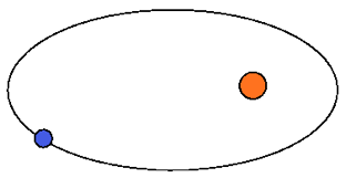
We treat the stars as point masses with positions . Writing and Newtons law of gravity provides the equation of motion
| (72) |
For simplicity we consider circular orbits constant, with the center of mass at rest. Conservation of angular momentum guarantees that the joint orbit lies in a plane, which we take to be the equatorial plane. Then the motion of the individual masses can be parametrized by
| (73) |
where the angular frequency is given in accordance with Keplers law by
| (74) |
For point masses the quadrupole moment is a sum of terms rather than an integral:
| (75) |
where is the reduced mass of the system. This expression for the quadrupole moment can now be substituted in eq. (71) to give the energy loss as
| (76) |
Observe, that one can also write this as
| (77) |
where denotes the corresponding Schwarzschild radius
| (78) |
The results obtained here can be applied for example to the case of binary neutron stars or white dwarfs; for equal mass systems
| (79) |
Now if this the gravitational energy flux is measured at a large distance on average the flux will be
| (80) |
We can compare this with the flux formula (51) for plane waves to get an estimate of the amplitude
| (81) |
where we have used the expression (74) for the frequency:
| (82) |
Equating the results (80) and (81) we get for the amplitude
| (83) |
For example two neutron stars of 1.4 solar mass each revolving around each other at a distance of km and observed from a distance of 6.4 kpc create gravitational waves of amplitude and frequency Hz.

These numbers are similar to those of the binary neutron star discovered in 1975 by Hulse and Taylor; they identified a pulsar which was part of a close binary system with a period of orbital revolution of about 7.5 hours. The masses of the stars were determined to be and and their distance to the solar system is kpc. Due to the emission of gravitational waves the orbit is expected to decay: the radius shrinks and the orbital period should decrease. As for this system the orbit is quite non-circular this change in period implies a shift in the periastron in addition to the one predicted by General Relativity for stable orbits around a star. Such a shift has been observed indeed over a period of more than 30 years, see figure 4; it is in close quantitative agreement with the expectations for gravitational wave emission [7]. The challenge this observation and similar later ones set is of course to detect these gravitational waves directly.
The result (77) also provides theoretical limit on the energy output of two revolving compact masses in gravitational radiation: as can never become smaller than we get
| (84) |
for two equal masses orbiting close to horizon distance. Apart from the fact that this limit presupposes the masses to be black holes, the estimate actually neglects all relativistic effects on the orbits as wel as radiation reaction. In practice the limit is actually more restrictive. Nevertheless the energy output can be enormous, up to 25 orders of magnitude larger than the present total energy output of the sun.
8 Observing gravitational waves
In view of the strong sources required and the small amplitudes involved the observation of gravitational waves is a major challenge. Common strategies to detect gravitational waves use apparatus exchanging energy with the wave field, either by absorption or emission. Two different strategies have been tried so far. The first one was the use of mechanical resonant oscillators, like solid bars or spheres. A second option is to use laser interferometry, either on the surface of the earth or in space. In addition there are strategies to establish the effects of gravitational waves on astronomical or cosmological phenomena, like the motion of pulsars or the imprint on the cosmic microwave background (CMB). We will briefly discuss some basic principles of these strategies. More detailed information is presented in the other lectures at this school and in the literature [5, 8, 9].
Resonant detectors
The first attempts to detect gravitational waves were made by J. Weber 45 years ago [12].
He equipped two massive aluminum cylinders with accelerometers at the end surfaces. When a
gravitational wave passes the apparatus, it will change its length by squeezing or stretching; if this
is done in resonance with the fundamental vibration mode of the cylinder the energy of vibration can
be changed. Subsequently a mechanical transducer can be used to amplify the change in amplitude
to a detectable level. Modern versions of these mechanical detectors operate at cryogenic temperatures
by cooling with liquid helium to reduce thermal noise. The best detectors have reached strain sensitivities
of about over a bandwidth of 1 Hz near the frequency of the fundamental mode, typically in
the range 900-1000 Hz. In spite of Weber’s original claims, no detection has ever been confirmed so far.
Interferometers
An interferometer consists of two –usually orthogonal– arms and a beam of light which is split at the
point where the arms join to create two beams traveling along each arm. At the end of the arms there
are mirrors reflecting the light beams back to the splitting point where the two beams can be compared
to find out differences in traveling time. The technical details are much more sophisticated, but this
description suffices for an understanding of the principles.
When a gravitational wave hits the interferometer the distances between the mirrors and the beam splitter change; the -polarization mode with respect to the axes defined by the lay-out of the interferometer, as sketched in figure 2, will cause one arm to become shorter and the other one longer. As a result the light beams arrive back at the splitter after a round trip at different times. In addition the collision with the accelerated mirror at the time of reflection creates a change in wavelength. The upshot is a measurable difference in phase and amplitude of the recombined light beams from which information about the amplitude and frequency of the gravitational wave can be reconstructed.
Large-scale interferometers presently operate in the USA: two LIGO detectors [13], and in Europe: VIRGO [14] an GEO-600 [15]. Similar devices are being planned elsewhere, e.g. in Japan and India. In the first round of operation LIGO and VIRGO reached typical strain sensitivities of in the frequency domain between 50-1000 Hz. Presently upgrades of the instruments are underway to improve these sensitivities by yet another order of magnitude.
Although these broad-band frequency sensitivities are quite impressive, unfortunately interferometers are mostly insensitive to the associated -polarization modes of gravitational-wave signals which create no difference in arrival times of the light beams. This also makes it very difficult to determine the polarization plane of the waves and their direction. Hence a single interferometer can detect a signal, but cannot identify its source. However by comparing the arrival times of signals at three interferometers not in the transversal polarization plane of the wave, it does become possible to obtain information about the direction of the wave and thus of its source. Therefore the existing large-scale interferometers mentioned above all combine data to allow for better and more accurate identification of gravitational wave signals.
Most resonant detectors actually suffer from the same problem of directional insensitivity, as the bar-type detectors also register a single polarization mode. An exception to this are spherical resonant detectors, like mini-Grail once operational at Leiden University [16], which was equally sensitive to all polarization modes and could in principle determine the direction of propagation of the wave.
Space based detectors
Terrestrial interferometers also suffer from the problem that they cannot operate at frequencies
below about 20 Hz due to seismic noise which drowns any signal. In particular the gravitational
waves emitted by the known binary pulsars, in the range of mHz and below, arre unobservable
with existing instruments. That problem could be solved by building a free-floating interferometer
in space. Plans for such an instrument exist at the European Space Agency. The eLISA project
[17] aims to bring three satellites carrying laser equipment in an orbit following the earth
around the sun. The distance between the satellites creating the arms of this interferometric type
of instrument will be about 1 000 000 km and be sensitive to gravitational waves with amplitudes
of in the mHz range from more or less anywhere in the universe. A first test with
instrumentation will be made during the Pathfinder mission to be launched in December 2015.
The actual mission of eLISA itself is scheduled in the years after 2030.
Pulsar timing
A completely different approach to observe very low frequency gravitational waves is offered by the
method of pulsar timing. Pulsars are rapidly spinning neutron stars emitting beams of radio-frequency
radiation rotating with the star. If the beam sweeps over the earth this results in extremely regular
pulses of radiowaves. As some pulsars spin at rates of several tens to several hundreds cycles
per second, pulsars act as millisecond clocks, which are actually stable to one part in a million or
better. Therefore pulsars can be used to keep time at the nanosecond level. Now the pulsars we
observe with such regularity are located in our galaxy, typically at distances of several hundreds of
parsecs (1 pc = 3.1 light years). Therefore the travel time of the radiosignals is of the order of
seconds. Thus in principle one can to determine variations in the travel time of the
signal of 1 part in - . By monitoring a sufficiently large set of pulsars
(typically 20-50) with this accuracy to get statistically significant data on the relative motion of
the pulsars with respect to earth it may become possible to discover variations due to the passage
of gravitational waves. This method has maximal sensitivity for waves in the frequency range of
- Hz, well below the eLISA range. It might be of importance to measure
gravitational radiation from binary supermassive black holes, which can be created in the merging
of galaxies. Several international research groups have started the timing of such pulsar networks;
they collaborate in the International Pulsar Timing Array network [18].
Polarization of the CMB
The cosmic microwave background is a diffuse thermal background of photons originating
from the time of formation of primordial neutral hydrogen and helium in the early universe,
when it was approximately 350 000 years old. Presently the average temperature of these
photons is 2.7 K which implies the spectrum peaks in the microwave range ( 100 GHz).
The density fluctuations in primordial matter have been measured with great precision from the
variations in temperature of the CMB over the sky. Gravitational waves from the early universe
would create tensor fluctuations in the CMB, resulting in polarization patterns known as
-modes: patterns with non-vanishing curl. Typically gravitational waves of primordial
origin visible years later in the CMB have frequencies of the order of Hz,
again orders of magnitude below those searched for by the pulsar timing arrays. One
experiment, BICEP2 located in Antarctica, has claimed to have detected evidence for -mode
polarization in the CMB [19], but this has not been confirmed by other observations
like those made by the Planck satellite mission [20].
9 Conclusions and outlook
We can summarize our findings as follows. The linear abelian spin-2 field theory in Minkowski space-time is a first-order approximation to fluctuations of the space-time metric in a near-Minkowski space-time. The fluctuations have two transverse polarization states and propagate at the speed of light and are identified with gravitational waves. The waves can be sourced by a time-variable quadrupole moment of matter and the intensity of such waves has been calculated. Even for strong and massive astrophysical sources the resulting amplitudes of gravitational waves are extremely small and will be detectable only with great effort.
We have discussed only the simplest case of gravitational waves in flat space-time. However, it is possible to proceed in analogous ways to calculate wave propagation in curved space-times, like cosmological geometries for an expanding universe or the strong-curvature regime of black holes [9, 10, 11]. Especially the merger phase of compact objects —white dwarfs, neutron stars or black holes— will produce strong and interesting wave signals from wich we can learn about gravity in the strong-field regime. Gravitational waves can even carry information about the earliest phase in the history of the universe before the universe became transparent to light or neutrinos.
Indirect evidence for the emission of gravitational waves by binary neutron stars is quite strong by now. It remains to observe this interesting phenomenon directly. Once the technology is in place a new era in astronomy and astrophysics will open.
Acknowledgements.
The work of the author is supported by the Foundation for Fundamental Reserach of Matter (FOM).References
- (1)
A. Einstein, Die Feldgleichungen der Gravitation
Sitzungsberichte der Preussischen Akademie der Wissenschaften zu Berlin (1915), 844 - (2)
A. Einstein, Die Grundlage der allgemeinen Relativitätstheorie
Annalen der Physik vierte Folge. Band 49 (1916) 769 - (3) S. Stevin, Beghinselen der Weeghconst (Plantijn; Leiden, 1586)
- (4)
M. Veltman, Quantum Theory of Gravitation, in: Methods in Field Theory
XXVIII Les Houches Summerschool, eds. R. Balian and J. Zinn-Justin (North-Holland, 1975) - (5) S. Weinberg, Gravitation and Cosmology (J. Wiley, 1972)
- (6) J.B. Hartle. Gravity, (Addison Wesley, 2003)
- (7)
J. M. Weisberg and J. H. Taylor
Relativistic Binary Pulsar B1913+16: Thirty Years of Observations and Analysis
in: Binary Radio Pulsars, Proc. Aspen Conference, ASP Conf. Series,
eds. F.A. Rasio & I.H. Stairs; arXiv:astro-ph/0407149 - (8)
P.R. Saulson, Fundamentals of Interferometric Gravitational Wave Detectors
(World Scientific, 1994) - (9) M. Maggiore, Gravitational Waves (Oxford Univ. Press, 2008)
- (10) K. Martel and E. Poisson, Gravitational perturbations of the Schwarzschild spacetime: a practical covariant and gauge-invariant formalism, Phys. Rev. D71 (2005), 104003
- (11)
G. Koekoek and J.W. van Holten,
Geodesic deviations: modeling extreme mass-ratio systems and their gravitational waves
Class. Quantum Grav. 28 (2011), 225022;
arXiv:1103.5612 [gr-qc] - (12) J. Weber, Gravitational-Wave-Detector Events, Phys. Rev. Lett. 20 (1968), 1307
- (13) The LIGO website: http://www.ligo.org
- (14) The VIRGO website: http://public.virgo-gw.eu
- (15) The GEO600 website: http://www.geo600.org
- (16) The miniGrail homepage: http://www.minigrail.nl
- (17) The eLISA homepage: http://www.elisascience.org
- (18) The International Pulsar Timing Array homepage: http://www.ipta4gw.org
- (19)
P.A.R. Ade et al.,
BICEP2 I: Detection Of B-mode Polarization at Degree Angular Scales
Phys. Rev. Lett. 112, 241101 (2014); arXiv:1403.3985 [astro-ph.CO] - (20)
The Planck Collaboration, Planck 2015 results. XIII. Cosmological parameters
arXiv:1502.01589 [astro-ph.CO]