Escape and trapping of low-frequency gravitationally lensed rays by compact objects within plasma
Abstract
We consider the gravitational lensing of rays emitted by a compact object (CO) within a distribution of plasma with power-law density . For the simplest case of a cloud of spherically symmetric cold non-magnetized plasma, the diverging effect of the plasma and the converging effect of gravitational lensing compete with one another. When , the plasma effect dominates over the vacuum Schwarzschild curvature, potentially shifting the radius of the unstable circular photon orbit outside the surface of the CO. When this occurs, we define two relatively narrow radio-frequency bands in which plasma effects are particularly significant. Rays in the escape window have and are free to propagate to infinity from the CO surface. To a distant observer, the visible portion of the CO surface appears to shrink as the observed frequency is reduced, and vanishes entirely at , in excess of the plasma frequency at the CO surface. We define the anomalous propagation window for frequencies . Rays emitted from the CO surface within this frequency range are dominated by optical effects from the plasma and curve back to the surface of the CO, effectively cloaking the star from distant observers. We conclude with a study of neutron star (NS) compactness ratios for a variety of nuclear matter equations of state (EoS). For , NSs generated from stiff EoS should display significant frequency dependence in the EW, and lower values of with softer EoS can also show these effects.
Keywords:
gravitation – plasmas – stars: neutron – pulsars: general1 Introduction
Gravitational lensing and plasma effects were first considered in the literature by Synge (1960), and later applied by Muhleman & Johnston (1966) and Muhleman, Ekers & Fomalont (1970), who calculated the effect of the solar plasma on the deviation of background starlight. The combination of gravitational lensing and plasma effects were significantly expanded on by Perlick (2000) and Bisnovatyi-Kogan & Tsupko (2009), leading to studies that range from the scale of stellar mass black holes in X-ray binaries (Bisnovatyi-Kogan & Tsupko, 2010) to galaxy-scale lenses (Er & Mao, 2014). This work has been extended to include rotation using the Kerr metric (Morozova, Ahmedov & Tursunov, 2013). The effect of plasma on the shadows of black holes in general relativity has also been explored (Atamurotov, Ahmedov & Abdujabbarov, 2015; Perlick, Tsupko & Bisnovatyi-Kogan, 2015; Abdujabbarov et al., 2016a), as well as near exotic objects (Abdujabbarov et al., 2015; Abdujabbarov et al., 2016b) and in gravity (Dastan, Saffari & Soroushfar, 2016). For a detailed overview of gravitational lensing effects within distributions of plasma, we refer to the thorough review provided by Bisnovatyi-Kogan & Tsupko (2015).
The plasma frequency defines a low-frequency cutoff for electromagnetic wave propagation. The index of refraction for radiation below this frequency is imaginary, which indicates that such low-frequency radiation is absorbed by the plasma. Generally the effect of plasma on ray trajectories near the compact object (CO) is expressed as an additional term in the effective potential. Kulsrud & Loeb (1992) showed that a constant plasma density provides an effective mass for light rays through this potential term. However, inhomogeneous distributions of plasma can generate more interesting effects (Tsupko & Bisnovatyi-Kogan, 2013). Rogers (2015) considered rays passing a massive object sheathed in a distribution of cold, non-magnetized plasma with a power-law density distribution for integer , and presented detailed calculations of the effect of the plasma with on the pulse profiles of a central neutron star (NS) with two emitting polar caps. Due to the dipolar magnetic field of the NS, the case was primarily investigated.
In this work, we investigate the consequences of low-frequency emission from a CO sheathed in plasma with . For this case, the plasma term in the effective potential drops off more slowly than the Schwarzschild vacuum term. When this occurs the diverging-lens behaviour of the plasma dominates for low-frequency rays, such that a potential maximum exists external to the stellar radius for sufficiently compact stars. Thus, low-frequency radiation is affected by turning points of the effective potential, causing rays which would usually escape the surface of the CO in the vacuum case to turn back towards the stellar surface. A wide range of other novel behaviour exists for rays that escape the CO surface with frequencies . We define this frequency range as the escape window (EW), and the trapped rays with are within the anomalous propagation window (APW). Ray trapping in the APW is analogous to the anomalous propagation of radio signals in the Earth’s atmosphere, and has profound effects on the appearance of a CO to distant observers, such as reducing the apparent radius of a CO as a function of frequency. In fact, the CO appears to vanish entirely as the observed frequency approaches , effectively ‘cloaking’ the stellar surface from a distant observer when observed at low frequencies. These frequency windows do not exist when the plasma density drops off more rapidly than the vacuum term in the effective gravitational potential for null geodesics in the Schwarzschild space–time.
We review the details of the geometrical optics approach to gravitational lensing within a plasma distribution in Section 2, provide the details of the frequency windows in Section 2.1 and derive the maximum impact parameter as a function of frequency in Section 2.2. We discuss our results in Section 3 and summarize our conclusions in Section 4.
2 Theory
Previous work (Rogers, 2015) examined modifications to ray trajectories introduced by a simple choice of dispersion relation in the case of spherical symmetry, following the general approach and notation of Tsupko & Bisnovatyi-Kogan (2013). We will briefly review the assumptions behind this physical scenario here.
We make use of the Schwarzschild metric to describe the space–time surrounding a spherically symmetric CO,
| (1) |
with the metric function
| (2) |
and abbreviating . In these definitions and for the rest of this paper, we use units which have . Let us assume the index of refraction for a cold plasma
| (3) |
with plasma frequency
| (4) |
that has a plasma particle charge and mass given by and , respectively, as well as the plasma number density . An often used plasma density in the literature is a radial power-law (Tsupko & Bisnovatyi-Kogan, 2013), such that
| (5) |
This puts the plasma frequency into a simple form,
| (6) |
where is a constant and is the power-law exponent. For simplicity, we set the constant in our numerical calculations. Throughout the text we refer to frequencies detected by a distant observer with the subscript , from the redshift relation
| (7) |
and do not explicitly state the radial dependence of . The Hamiltonian for rays in curved space–time and under the effects of an optical medium with index of refraction (Synge, 1960) using cold non-magnetized plasma is
| (8) |
The equations of motion are given in terms of an arbitrary curve parameter :
| (9) |
| (10) |
From these relationships equation 10 immediately gives
| (11) |
The vanishing derivatives show that the , and components must be constant. By spherical symmetry, we choose to work in the equatorial plane so take . The and quantities are interpreted as the energy and angular momentum of a ray,
| (12) |
and
| (13) |
where is the impact parameter of an escaping ray. Finally, the derivative of the radial momentum is
| (14) |
We can find an expression for the radial momentum directly from the vanishing of the Hamiltonian, such that
| (15) |
and the sign of depends on the ray trajectory, with positive indicating an outgoing ray and negative for an incoming ray. The coordinate derivatives using equation 9 give
| (16) |
| (17) |
| (18) |
and working in the equatorial plane implies
| (19) |
For an initial position , ray energy and angular momentum , as well as a choice of sign for , equations 11 to 19 form a system of equations that are easily solved using an integration scheme for second-order ordinary differential equations, such as the fourth-order Runge–Kutta method. The solution to this system gives points along the path of a ray trajectory launched from in the direction of our choice. We stop integration when the ray returns to the surface of the CO (), or when it escapes to a sufficiently great distance ().
The trajectory of a ray near the CO is described in terms of an effective potential. We denote , and use equations 15 and 17 to give an energy conservation equation
| (20) |
with
| (21) |
where the vacuum contribution is the first term in the square brackets and the second term is entirely due to the plasma. Setting the square of the ray energy equal to the effective potential gives the propagation condition
| (22) |
which must be satisfied at every point along the trajectory for rays to escape from the surface of the CO and travel to infinity. The impact parameter of an escaping ray with asymptotic frequency is
| (23) |
This ray will intersect the radial normal vector at with an angle . A ray passing with a grazing incidence and escaping to reach an observer at infinity defines the maximum impact parameter, at a particular frequency. All rays that pass with impact parameter will intersect at smaller angles.
In analogy to equation 7, we use the effective redshift formula to define the plasma frequency at infinity,
| (24) |
where is the position of the maximum density along the path of a given ray. The rays that propagate through plasma that are visible to distant observers require everywhere along their trajectory. Note that the plasma frequency at infinity is equivalent to the square root of the effective potential (equation 21) with . This means that radially directed rays with sufficiently low asymptotic frequency will be absorbed since the index of refraction vanishes for rays at the asymptotic plasma frequency. These rays have absorption points rather than turning points. However, rays with finite at these same frequencies can propagate freely since they remain above the plasma frequency cutoff at all times due to the contribution of to the effective potential.
2.1 Frequency windows
For plasma density distributions with power-law index , the propagation of low-frequency rays is complicated by the presence of a turning point that can be external to the stellar surface. The dependence between the radius of the photon sphere and was discussed by Perlick, Tsupko & Bisnovatyi-Kogan (2015) in their work on black hole shadows in plasma. However, the effect has additional implications for objects with surfaces that produce low-frequency emission.
We define the EW as a range of frequencies within which rays are strongly affected by the plasma, but are still free to escape to an observer at infinity. At , the effective potential allows a circular orbit at the exact surface of the CO for the maximum impact parameter given by equation 23 with . This condition remains valid for higher frequencies as these have circular orbit radii within the stellar surface. At the lower limit of the EW only the fiducial ray with frequency escapes to a distant observer.
To describe these effects quantitatively, let the circular orbit radius be called , the position of the potential maximum where the derivative of the effective potential vanishes. This condition gives the critical angular momentum required for a circular orbit in terms of ,
| (25) |
with in terms of the observed frequency at infinity, and we write the critical impact parameter as . The upper frequency limit of the EW is found when the circular orbit and stellar surface coincide at , with the corresponding angular momentum , and . Above this limit, , the circular orbit is within the stellar surface and all rays are generally free to escape to infinity with maximum impact parameter . For this reason, we will restrict ourselves to cases for which , in which ray paths are significantly altered from their vacuum behaviour. The angular momentum can be used to define a corresponding asymptotic frequency which we call the upper limit of the EW, . With the effective potential (equation 21), and using the equality in the propagation condition (equation 22), we find an expression for the corresponding asymptotic frequency
| (26) |
From this expression, we see that the upper frequency limit vanishes when , and real values of the upper frequency limit exist only for plasma distributions with .
Rays with frequencies can enter a circular orbit outside the CO surface. The presence of the unstable circular orbit external to the stellar surface implies a maximum in the potential. Therefore a ray escaping the CO surface must have energy in excess of this maximum to escape and avoid a turning (absorption) point in the trajectory. Thus, the effective potential maximum defines the lower limit of the EW, , which a distant observer detects as an asymptotic frequency
| (27) |
This is the threshold frequency for rays to escape the stellar surface.
The existence of the EW provides a constraint on the maximum compactness ratio of a CO, . Let us consider a radially directed ray () that is at the threshold of escape. Equation 25 vanishes for a ray that is radially directed. With this condition the position of the potential maximum for general is
| (28) |
The existence of a turning point at or external to the CO surface is necessary for the existence of the EW. Let us set for the most conservative limiting case. Combined with the condition implied by equation 26, we find a minimum compactness ratio
| (29) |
This compactness ratio is a realistic lower bound for NSs, which we will discuss further in Section 3.
Finally, we also note the simplification introduced for radially directed rays at the minimum EW frequency . Using equation 28 in equation 27 gives the lower EW limit for a radially directed ray,
| (30) |
In the specific case and ,
| (31) |
This is the minimum frequency limit for rays to escape along a radial trajectory, and equals the asymptotic plasma frequency (equation 24).
For rays with frequencies lower than the EW, we define the APW, in which the diverging effect of the plasma dominates ray propagation. The APW is the range of frequencies given by . Since implies a potential maximum of , the APW is bounded from below by
| (32) |
Rays in the APW that are emitted by the CO have frequencies larger than the local plasma frequency for radii , but below the asymptotic plasma frequency at required for escape. Thus, these rays are effectively trapped in the environment of the CO. Rays in the APW reach a maximum distance where they encounter a turning point due to the potential barrier and subsequently reverse direction to curve back to the CO surface. Rays external to the circular orbit radius with frequencies in the APW that approach the CO from infinity reach a minimum turning distance and are reflected away from the CO by the potential boundary, returning to infinity. To find the external turning radius as a function of impact parameter, let us consider the polynomial expression for the turning points (Rogers, 2015),
| (33) |
For a given , the solutions of equation 33 give the external turning points . For rays emitted from the surface of the CO in the APW, we substitute to find the corresponding interior turning points in terms of . The simplest example is a radially directed ray. Using and setting eliminates the terms, giving
| (34) |
However, as seen from the effective potential and equation 24, radially outgoing rays experience absorption at the turning points due to the plasma frequency. Thus, rays are absorbed at , but all other rays with non-vanishing are free to propagate.
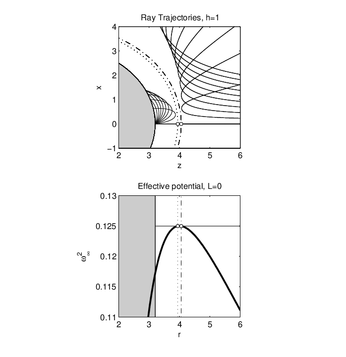
We demonstrate the behaviour of trapped and deflected rays in the APW in Fig. 1. In this and the remainder of the examples in this work we assume and use with . We assume a ray frequency near the ceiling of the APW, . The top panel of this figure illustrates trajectories that are emitted from the CO surface with varying from to in increments of . The fiducial radially directed rays with reach , marked as a dotted circle and are absorbed. The exact position of the absorption point of the fiducial ray is marked as an open circle. Rays with finite reach a maximum altitude and turn back to the CO. The exterior rays which are turned away from the CO are shown with impact parameters , using the corresponding angular momenta for the interior rays. These trajectories turn away from the CO. The closest approach for the fiducial ray is marked as a dash–dotted circle, and the absorption point is explicitly marked for the external fiducial ray. The other rays are turned away from the CO and return to infinity.
The effective potential for the fiducial rays is shown in the lower panel of Fig. 1 as the thick curved line. The fiducial rays are represented by the horizontal thin lines, with the absorption points marked as open circles, and the corresponding radii marked with vertical dotted and dash–dotted lines. The interior of the CO is shown in both panels by the light grey area. Thus, when observed at frequencies within the APW (), the CO is effectively ‘cloaked’ from detection by distant observers.
2.2 Maximum impact parameter for rays within the EW
The maximum impact parameter for rays at and above the high-frequency end of the EW is found by setting in equation 23,
| (35) |
with emission angle for a ray that makes a grazing escape from the CO surface. However, for COs sheathed in power-law distributions of plasma with , frequencies in the EW have the maximum impact parameter reduced since . At , the maximum impact parameter for rays to escape vanishes entirely, and the image of the stellar surface to a distant observer appears to be a single point. We call the maximum impact parameter in the EW .
In general, the maximum impact parameter is the limiting case for which equation 33 has a single solution. A ray with maximum impact parameter () will enter the circular orbit at . Thus, the maximum impact parameter is found by evaluating equation 23 at ,
| (36) |
However, this expression presents a difficulty since solving for from the potential derivative requires the angular momentum , which itself is limited by for escaping rays at a particular frequency. Therefore, we propose to use the turning point relationship (equation 33) directly to discover the maximum impact parameter given only and without a priori knowledge of explicitly.
For general , the solution of the turning point equation must be found using numerical methods since terms with fractional exponents will be present. Analytical solutions exist for integer values of , however the homogeneous case simply reproduces the behaviour of a massive particle with mass (Kulsrud & Loeb, 1992), though the general procedure used below can also provide the analytical solution. For the remainder of this section we examine the case, for which equation 33 reduces to a cubic with the general form
| (37) |
A unique solution for this equation can be found by enforcing the discriminant to vanish. This discriminant condition results in a second cubic equation in , solved by standard methods (Holmes, 2002). To state the solution explicitly, we define
| (38) |
| (39) |
| (40) |
along with
| (41) |
and
| (42) |
In terms of these quantities, the maximum impact parameter that causes the discriminant to vanish is
| (43) |
When the function is given in terms of hyperbolic functions (Holmes, 2002). For and ,
| (44) |
and for ,
| (45) |
With the maximum impact parameter we find the corresponding angular momentum for a given frequency, , and the critical radius follows. Numerical evaluation confirms that equations 43 and 36 produce identical results.
The angle that a ray with the maximum impact parameter makes with respect to the normal direction at the stellar surface is
| (46) |
This shows that near , rays that escape have small and are close to the radial direction . As the observed frequency increases, rays arriving at the observer will leave the CO at increasing angles, with the maximum at the top of the EW. We show rays with impact parameter for frequencies ranging logarithmically across the EW using the radial limit of (equation 30) to for in Fig. 2.

We demonstrate how elements of the CO surface appear on the sky of a distant observer in Fig. 3. In the top panel of this figure, we launch rays from the surface of the CO to an observer located a great distance away in the direction. For illustrative purposes we choose four frequencies in the EW, which we parametrize as , where is the width of the EW, and ranges from to . For convenience, we will refer to these frequencies simply in terms of . We choose to have the arbitrary values , , and , respectively. For each of these frequencies, we find the maximum impact parameter and consider the arbitrary impact parameter to avoid the circular orbit at . These rays are illustrated in the top panel of Fig. 3 and increase in from the fiducial ray in the direction. Let us then define the angle between the position of the ray on the stellar surface and the fiducial direction as the surface angle. To illustrate the effect that the plasma has on the appearance of a CO to a distant observer, we shade each of the surface angle elements in the top panel of Fig. 3 with an alternating light dark scheme. Due to spherical symmetry these surface regions define shaded rings on the surface of the CO concentric with respect to the line of sight. The surface angle regions contain all impact parameters . We plot these regions as a series of concentric discs on the lower panels. For each frequency, the surface angle regions are projected to the observer’s sky. These plots show how the plasma distorts the view of the CO as a function of frequency.
For , the surface of the CO appears pointlike, and at the large surface angle regions occupy a narrow range of large impact parameters and appear extremely compressed to the observer, subtending a small region at the limb of the CO disc. These areas subtend a larger solid angle on the sky as the frequency is increased. The and frequencies most clearly illustrate this point. Despite the maximum impact parameter for the and rays subtending nearly the same angle over the surface of the CO (i.e. in the top panel of Fig. 3), these regions project to different solid angles on the sky as seen in the bottom row of the figure. In these panels, the exterior dark grey ring represents the same region of the CO surface but it is markedly smaller in the panel with respect to the other solid angle elements. This shows that increasing the frequency does not simply scale the view of the CO surface to a larger size, but changes the proportions of the visible surface angle elements relative to one another. The demagnifying nature of the relativistic images produced by COs is well known and has been extensively studied in the lensing literature (Virbhadra & Ellis, 2000; Virbhadra, 2009), as well as in studies of the solid angles of NS surface elements projected to an observer in vacuum conditions (Pechenick, Ftaclas & Cohen, 1983; Dąbrowski & Osarczuk, 1995).

We show the evolution of the pulse profile as a function of frequency in Fig. 4. The pulse profile is calculated using the method from Rogers (2015), with a single isotropically emitting radio-loud cap on the CO surface that has angular radius centred on the pole. The pole is set to an angle with respect to the rotation axis. This configuration aligns the line of sight and the centre of the polar cap at , where is the rotation frequency of the CO. The cap is on the opposite side of the star at . All other properties are as in Fig. 3. The curves show the evolution of the pulse profile with frequency. The large peak that occurs when the polar cap is facing away from the viewer in the vacuum case is due to multiple imaging of the cap as rays are bent around the CO. In this configuration, the polar cap appears to the observer as a bright ring around the periphery of the NS. As the visible surface area decreases with frequency, the magnitude of this peak is correspondingly reduced. At the bottom of the EW, , the pulse profile vanishes entirely. In addition to the frequency-dependent pulse morphology, the propagation of beamed pulsar radiation through plasma also results in a frequency-dependent time delay, which is strongly affected by the plasma properties (Rogers, 2015).

3 Discussion
In the analytical examples worked in the previous sections, we have assumed a CO with , slightly larger than the vacuum photon sphere at . Since we find the location of a turning point with , the maximum possible compactness of a CO is relevant. To address the question of how compact a CO can be, we examined parametrized analytical fits to separate equations of state (EoS) for neutron matter (Gungor & Eksi, 2012) that include a large cross-section of unique physics ranging from conventional npe matter to hybrid stars that possess exotic baryon condensates in their cores. For each of these EoS fits, we solve the Tolman–Oppenheimer–Volkov equations (Glendenning, 2000) to derive the mass–radius relationship. We also additionally include two examples for strange stars, based on perturbative QCD calculations (Fraga, Pisarski & Schaffner-Bielich, 2001; Orsaria et al., 2011). The WFF1 equation of state (Wiringa, Fiks & Fabrocini, 1988; Gungor & Eksi, 2012) gives the smallest compactness ratio at above our lower limit of found from equation 29. This implies that highly compact NSs that are sheathed in power-law distributions of plasma can allow for the frequency effects studied in Section 2 provided that the plasma density drops off slowly enough (). The soft EoS that produces COs with requires to show joint effects from gravitational lensing and plasma. While our results focus specifically on the power-law case, the frequency windows exist for any plasma distribution with density that drops off sufficiently slowly.
The case has particular relevance for the study of pulsar wind nebulae. An aligned rotating NS produces a particle wind with a density that is proportional to (Contopoulos, Kazanas & Fendt, 1999; Harding, Contopoulos & Kazanas, 1999; Kirk, Lyubarsky & Petri, 2009; Tong, Xu, Song & Qiao, 2013). Provided radio emission from low altitudes in the pulsar magnetosphere (Hassall et al., 2012; Jones, 2016a), both general relativistic effects and the refractive index of the magnetospheric plasma may be relevant. These effects may also be significant for models of eclipsing binary NSs or NS-black hole systems that are nearly edge-on with respect to the observer (Keane et al., 2015; Shao et al., 2015).
Finally, let us consider the ratios of the upper and lower EW limits with respect to the plasma frequency. For the cases with , the asymptotic value of the plasma frequency is calculated with respect to the stellar surface. Evaluating equation 24 at the stellar surface gives
| (47) |
However, when , the circular orbit radius is external to the stellar surface, . The propagation condition requires that observable rays have frequency in excess of the asymptotic plasma frequency in order to escape the CO. Thus, for the asymptotic plasma frequency must be evaluated with respect to the circular orbit radius at the potential maximum. Since the most significant observable effects due to the plasma occur within the EW, it is of interest to compare the enhancement of the EW limits with respect to the asymptotic plasma frequency evaluated at the surface of the CO. Using equations 26 and 24 we find
| (48) |
For a radially directed ray, we use equation 30 to find
| (49) |
Note that besides the mass and radius of the CO, the ratios depend only on the power-law exponent, such that the specific details of the plasma contained in the constant drop out entirely.
As an example, let us return to the case with and a compactness ratio . With these parameters, we use equation 49 to find the lower limit of the EW at and equation 48 evaluates to . In Rogers (2015), we estimated an upper limit of the plasma frequency of the order of MHz, which is boosted to MHz from the effects presented in this work. Within this frequency range the pulse profiles should be drastically affected as shown in Fig. 4. While the increase in the cutoff frequency for is modest, in the limit the limiting frequency ratio over the EW varies between and , a moderate boost compared to the plasma frequency cutoff at the stellar surface. Therefore, due to the increase in the frequency range of the EW from a potential maximum external to the CO surface, the combined action of plasma and gravitational effects may occur in COs at slightly higher frequencies than previously estimated in the literature (Bisnovatyi-Kogan & Tsupko, 2015; Rogers, 2015). Despite this modification, the values above represent a rough estimate since relativistic plasma in a pulsar magnetosphere must have a plasma frequency MHz (Gedalin, Melrose & Gruman, 1998; Melrose & Gedalin, 1999; Jones, 2016b).
The calculations in Section 2 and the pulse profiles shown in Fig. 4 are a first approximation. In general, we expect other significant factors must also be taken into account to describe real COs. The assumption that pulsed radio emission occurs near the surface is most reasonable for millisecond pulsars with small magnetospheres (Gil & Kijak, 1993; Kijak & Gil, 1998) and rapid rotation that causes distortions of the pulse profile through the Doppler effect (Cadeau et al., 2007). We have also treated the plasma as cold and ignored the magnetic field; however, both of these factors should play a significant role in describing the distribution of plasma within the magnetosphere and the propagation of electromagnetic radiation through it (Kulsrud & Loeb, 1992; Gedalin & Melrose, 2001; Petrova, 2002). A complete description requires the full treatment of covariant radiative transfer, derived in Broderick & Blandford (2003a) and Broderick & Blandford (2004). In fact, polarized emission can be used as a probe of the plasma density around X-ray binaries and pulsars (Broderick & Blandford, 2003a).
The narrow, low-frequency bands required to observe pulse profiles provide the greatest challenge to detecting the effects described in this work directly. However, there are a number of instruments suited to studying the low-frequency pulsed emission and time delays required, in particular the Low-Frequency Array (van Haarlem et al, 2013, LOFAR;), which observes in the frequency range – MHz (Stappers et al., 2011), the Long Wavelength Array between and MHz (Stoval et al., 2015, LWA;), the Ukrainian T-shaped Radio Telescope in the range of – MHz (Zakharenko et al., 2013, UTR-2;) and the Murchison Widefield Array between and MHz (Tremblay et al., 2015, MWA;). Extremely low frequency observations ( MHz) are complicated by a number of effects, including scattering from the interstellar medium, radio frequency interference from man-made sources and transmission through the Earth’s atmosphere. Below MHz radio signals are completely attenuated by ionospheric propagation effects. Despite these difficulties, anomalous X-ray pulsars have been studied at – MHz (Malov & Malofeev, 2010; Malov, 2014), and a large sample of pulsar light curves have been studied over a broad range of frequencies by LOFAR (Bilous et al., 2016; Kondratiev et al., 2016), down to as low as MHz (Pilia et al., 2016). Generally, a low-frequency turnover in the spectrum of radio pulsars is associated with a corresponding evolution of the pulse profile, related to processes occurring near the rest-frame plasma frequency above the polar cap (Sieber, 1970; Malofeev & Malov, 1980). While many NSs do not show evidence of such a turnover (Bilous et al., 2016; Kondratiev et al., 2016), this feature has been identified in a number of objects. For our purposes, we focus on the pulsars with a low-frequency turnover, such as PSR B1133+16 (Jones, 2013), the millisecond pulsars J2145–0750 (Kuzmin & Losovsky, 1996; Stappers, 2008; Dowell et al., 2013; Kuniyoshi et al., 2015) and J1012+5307 (Kuzmin & Losovsky, 2001; Kondratiev et al., 2016), as well as a handful of additional systems (Kuniyoshi et al., 2015; Kondratiev et al., 2016, see for example). We do not suggest that lensing and plasma effects account for these observations in their entirety, but if components of the radio beam arise from emission near the surface of the NS, these components can be affected by joint effects of gravity and the surrounding plasma environment.
The Square Kilometre Array (Karastergiou et al., 2015, SKA;) is projected to be in operation by 2020. The sensitivity of the SKA will be vital for studying the emission properties of PSRs and detecting new systems. However, extreme measures are required to overcome the fundamental limitations of low-frequency observations imposed by artificial and ionospheric sources of radio interference. A proposed solution has been to place an antenna array composed of a swarm of satellites in a lunar orbit (Bergman et al., 2009; Boonstra et al., 2010; Baan et al., 2012; Rajan et al., 2016). In principle, such a space-based radio telescope could be sensitive to ultralow frequencies in the range kHz– MHz, opening a new avenue of inquiry into the emission processes active in NSs.
4 Conclusions
In the vacuum case, all frequencies of electromagnetic waves are affected equally by the lensing effects of the Schwarzschild metric. However, for a power-law distribution of plasma in the curved space–time around a CO, the issue of whether a star is observable at a particular frequency is more subtle, since the apparent radius of the star is frequency dependent with respect to a distant observer.
To quantify the behaviour of rays as a function of frequency, we defined two frequency windows for power-law plasma distributions with : the EW is the window in which rays originating from the CO surface can escape to a distant observer, , and the APW spans the frequency range . In the APW, a family of rays exist that are emitted from and return to the CO surface. These behaviours are dependent on the presence of a plasma that drops off more slowly than the contribution from the vacuum term in the effective potential. The frequency windows are found analytically for power-law distributions and have analytical expressions for integer , but must be solved numerically for non-integer values. The maximum impact parameter for rays in the EW is given as a function of frequency from analysis of the classical turning points of the effective potential.
Finally, we studied plasma effects on the appearance of a CO formed on the sky of a distant observer. For a range of angles on the surface of a CO, we found the corresponding projection on the observer’s sky. The solid angle subtended by the CO appears to change apparent size when the observing frequency is increased. At frequencies much larger than the upper limit of the EW, vacuum behaviour is recovered.
Acknowledgements
It is my pleasure to acknowledge and thank Samar Safi-Harb for support through the Natural Sciences and Engineering Research Council of Canada (NSERC) Canada Research Chairs Program. I acknowledge Xinzhong Er for many interesting discussions and helpful comments that improved the clarity and flow of this manuscript, and thank Charlene Pawluck for proofreading and helpful suggestions for improving the text. I also acknowledge and thank the anonymous referee for providing valuable feedback that improved the manuscript.
References
- Abdujabbarov et al. (2015) Abdujabbarov A., Toshmatov B., Stuchlik Z., Ahmedov B., 2015, preprint (arXiv:1512.05206)
- Abdujabbarov et al. (2016a) Abdujabbarov A., Amir M., Ahmedov B., Ghosh S., 2016a, Phys. Rev. D, 93, 10
- Abdujabbarov et al. (2016b) Abdujabbarov A., Juraev B., Ahmedov B., Stuchlik Z., 2016b, Ap&SS, 361, 7
- Atamurotov, Ahmedov & Abdujabbarov (2015) Atamurotov F., Ahmedov B., Abdujabbarov A., 2015, Phys. Rev. D, 92, 084005
- Baan et al. (2012) Baan W., 2012, Proc. Sci., Vol. 1, From Antikythera to the Square Kilometre Array: Lessons from the Ancients, SISSA, Trieste, PoS(Antikythera & SKA)045
- Bergman et al. (2009) Bergman J. E. S., Blott R. J., Forbes A. B., Humphreys D. A., Robinson D. W., Stavrinidis C., 2009, CEAS 2009, preprint (arXiv:0911.0991)
- Bilous et al. (2016) Bilous A. V. et al. 2016, A&A, 591, A134
- Bisnovatyi-Kogan & Tsupko (2009) Bisnovatyi-Kogan G. S., Tsupko O. Yu., 2009, Gravit. Cosmology, 15, 20
- Bisnovatyi-Kogan & Tsupko (2010) Bisnovatyi-Kogan G. S., Tsupko O. Yu., 2010, MNRAS, 404, 1790
- Bisnovatyi-Kogan & Tsupko (2015) Bisnovatyi-Kogan G. S., Tsupko O. Yu., 2015, Plasma Phys. Rep., 41, 562
- Boonstra et al. (2010) Boonstra A.-J., Saks N., Bentum M. J., van’t Klooster K., Falcke H., 2010, in Proc. 61st Int. Astron. Congress, Vol. 10, p. 8036
- Broderick & Blandford (2003a) Broderick A., Blandford R., 2003, MNRAS, 342, 1280
- Broderick & Blandford (2004) Broderick A., Blandford R., 2004, MNRAS, 349, 994
- Cadeau et al. (2007) Cadeau C., Morsink S. M., Leahy D., Campbell S. S., 2007, ApJ, 654, 458
- Contopoulos, Kazanas & Fendt (1999) Contopoulos I., Kazanas D., Fendt C., 1999, ApJ, 511, 351
- Dastan, Saffari & Soroushfar (2016) Dastan S., Saffari R., Soroushfar S., 2016, preprint (arXiv:1606.06994)
- Dąbrowski & Osarczuk (1995) Dąbrowski M. P., Osarczuk J., 1995, Ap&SS, 229, 139
- Dowell et al. (2013) Dowell J. et al., 2013, ApJ, 775, L28
- Er & Mao (2014) Er X., Mao S., 2014, MNRAS, 437, 2180
- Fraga, Pisarski & Schaffner-Bielich (2001) Fraga E. S., Pisarski R. D., Schaffner-Bielich J. S. 2001, Phys. Rev. D, 63, 12, 121702
- Gedalin & Melrose (2001) Gedalin M., Melrose D. B., 2001, Phys. Rev. E, 64, 027401
- Gedalin, Melrose & Gruman (1998) Gedalin M., Melrose D. B., Gruman E., 1998, Phys. Rev. E, 57, 3399
- Gil & Kijak (1993) Gil J. A., Kijak J., 1993, A&A, 273, 563
- Glendenning (2000) Glendenning N. K., 2000, Compact Stars - Nuclear Physics, Particle Physics, and General Relativity. Springer, New York
- Gungor & Eksi (2012) Gungor C., Eksi K. Y. 2012, in Capuzzo Dolcetta R., Limongei M., Tomambe A., Giobbi G. eds., Proc. Advances in Computational Astrophysics: Methods, Tools and Outcomes, Cefaulu, Sicily, Italy
- Harding, Contopoulos & Kazanas (1999) Harding A. K., Contopoulos I., Kazanas D., 2013, ApJ, 525, L125
- Hassall et al. (2012) Hassall T. E. et al. 2012, A&A 543, A66
- Holmes (2002) Holmes G. C. 2002, Math. Gaz., 86, 473
- Jones (2013) Jones P. B., 2013, MNRAS, 435, L11
- Jones (2016a) Jones P. B., 2016a, MNRAS, 455, 3814
- Jones (2016b) Jones P. B., 2016b, MNRAS, 459, 3307
- Karastergiou et al. (2015) Karastergiou A. et al., 2015, in Bourke T. L. et al., eds, Proc. Sci., Advancing Astrophysics with the Square Kilometre Array (AASKA14), Giardini Naxos, Italy, 38
- Keane et al. (2015) Keane E. F. et al. 2015, in Bourke T. L. et al., eds, Proc. Sci., Advancing Astrophysics with the Square Kilometre Array (AASKA14), Giardini Naxos, Italy, 40
- Kijak & Gil (1998) Kijak J., Gil J. A., 1998, MNRAS, 299, 855
- Kirk, Lyubarsky & Petri (2009) Kirk J. G., Lyubarsky Y., Petri J., 2009, in Becker W., ed, Astrophysics and Space Science Library, Vol. 357, Neutron Stars and Pulsars. Springer, Berlin, p. 697
- Kondratiev et al. (2016) Kondratiev V. I. et al., 2016, A&A, 585, A128
- Kulsrud & Loeb (1992) Kulsrud R., Loeb A., 1992, Phys. Rev. D, 45, 525
- Kuniyoshi et al. (2015) Kuniyoshi M., Verbiest J. P. W., Lee K. J., Adebahr B., Kramer M., Noutsos A., 2015, MNRAS, 453, 828
- Kuzmin & Losovsky (1996) Kuzmin A. D., Losovsky B. Y., 1996, A&A, 308, 91
- Kuzmin & Losovsky (2001) Kuzmin A. D., Losovsky B. Ya., 2001, A&A, 368, 230
- Malofeev & Malov (1980) Malofeev V. M., Malov I. F., 1980, Astron. Zh., 1, 90
- Malov (2014) Malov I. F., 2014, Astron. Rep., 58, 733
- Malov & Malofeev (2010) Malov O. I., Malofeev V. M., 2010, Astron. Rep., 54, 210
- Melrose & Gedalin (1999) Melrose D. B., Gedalin M. E., 1999, ApJ, 521, 351
- Morozova, Ahmedov & Tursunov (2013) Morozova V. S., Ahmedov B. J., Tursunov A. A., 2013, Ap&SS, 346, 513
- Muhleman & Johnston (1966) Muhleman D. O., Johnston I. D., 1966, Phys. Rev. Lett., 17, 455
- Muhleman, Ekers & Fomalont (1970) Muhleman D. O., Ekers R.D., Fomalont E. B., 1977, Phys. Rev. Lett., 24, 1377
- Orsaria et al. (2011) Orsaria M., Ranea-Sandoval I. F., Vucetich H., 2011, ApJ, 734, 41
- Pechenick, Ftaclas & Cohen (1983) Pechenick K. R., Ftaclas C., Cohen J. M., 1983, ApJ, 274, 846
- Perlick (2000) Perlick V., 2000, Ray Optics, Fermat’s Principle and Applications to General Relativity. Springer-Verlag, Heidelberg
- Perlick, Tsupko & Bisnovatyi-Kogan (2015) Perlick V., Tsupko O. Yu., Bisnovatyi-Kogan G. S., 2015, Phys. Rev. D., 92, 104031
- Petrova (2002) Petrova S. A., 2002, A&A, 383, 1067
- Pilia et al. (2016) Pilia M. et al. 2016, A&A, 586, A92
- Rajan et al. (2016) Rajan R. T., Boonstra A.-J., Bentum M., Klein-Wolt M., Belien F., Arts M., Saks N., van der Veen A.-J., 2016, Exp. Astron., 41, 271
- Rogers (2015) Rogers A. 2015, MNRAS, 451, 17
- Shao et al. (2015) Shao L. et al. 2015, in Bourke T. L. et al., eds, Proc. Sci., Advancing Astrophysics with the Square Kilometre Array (AASKA14), Giardini Naxos, Italy, 42
- Sieber (1970) Sieber W., 1970, A&A, 28, 237
- Stappers (2008) Stappers B. W., Karappusamy R., Hessels J. W. T., 2008, in Bassa C., Wang Z., Cumming A., & Kaspi V. M. eds, AIP Conf. Proc. Vol. 983, 40 Years of Pulsars: Millisecond Pulsars. Am. Inst. Phys., New York, p. 593
- Stappers et al. (2011) Stappers B. W. et al., 2011, A&A, 530, A80
- Stoval et al. (2015) Stovall K. et al. 2015, ApJ, 808, 156
- Synge (1960) Synge J. L., 1960, Relativity: The General Theory. North-Holland, Amsterdam
- Tong, Xu, Song & Qiao (2013) Tong H., Xu R. X., Song L. M., Qiao G. J., 2013, ApJ, 768, 144
- Tremblay et al. (2015) Tremblay, S. E. et al. 2015, PASA, 32, 5
- Tsupko & Bisnovatyi-Kogan (2013) Tsupko O. Y., Bisnovatyi-Kogan G. S., 2013, Phys. Rev. D, 87, 124009
- van Haarlem et al (2013) van Haarlem M. P. et al., 2013, A&A, 556, A2
- Virbhadra (2009) Virbhadra K. S. 2009, Phys. Rev. D, 79, 083004
- Virbhadra & Ellis (2000) Virbhadra K. S., Ellis G. F. R. 2000, Phys. Rev. D, 62, 084003
- Wiringa, Fiks & Fabrocini (1988) Wiringa R. B., Fiks V., Fabrocini A., 1988, Phys. Rev. C, 38, 1010
- Zakharenko et al. (2013) Zakharenko V. V. et al., 2013, MNRAS, 431, 3624