A field theory can sometimes be approximated by a simpler, so-called ”effective” theory, in a given region of phase space. ¹¹ 1 One often encounters low-energy effective theories in the literature, but there are other regions of phase space where an effective theory approach can be used. For example, an effective theory for singlet resonances has been described in [8]. Consider an ultraviolet (UV) theory that lies at a scale $\Lambda$ which is much larger than the typical energy scale $E$ of a given experiment $(\Lambda\gg E)$. From the UV point of view, the low-energy effective theory is obtained by expanding the correlation functions computed within the UV theory with respect to the parameter $E/\Lambda$.

It is very plausible that the Standard Model is not the ultimate UV-complete theory of nature and its Lagrangian corresponds to the relevant and marginal sector of a low-energy effective theory. In this picture, the full SM effective Lagrangian also contains a series of operators of dimension higher than four, built from SM fields and invariant under SM symmetries, which are suppressed by inverse powers of the new physics scale $\Lambda$. To the low-energy observer, these higher dimensional operators parametrize the new physics effects, which appear as new interactions between the known particles, including vertices with extra derivatives. The SM effective Lagrangian takes the general form

where

The effective operators $\mathcal{O}_{I}^{(d)}$ have mass dimension $d>4$ and $\alpha_{I}^{(d)}$ are dimensionless coefficients. In general, these coefficients can be complex, depending on the operator. However one can always split the operator into its real and imaginary parts in order to end up with only real coefficients. Because of this, in the following we will consider only real coefficients, without loss of generality.

Identifying $\Lambda$ with the mass scale of a heavy particle, the effective field theory is valid only at energies

and the contributions of the effective operators to any given observable are arranged as an expansion in $E/\Lambda$. ²² 2 Another bound comes from requiring a perturbative expansion of the effective interactions, which implies $$\frac{|\alpha|}{\Lambda^{2}}<\frac{4\pi}{E^{2}}\,.$$ (4) Moreover, requiring perturbative couplings in the UV theory implies a bound on $\alpha$, that depends on the number of fields $n$ in the effective operator (or equivalently to the number of legs of the corresponding UV amplitudes). For dimension-6 operators one has $$|\alpha|<(4\pi)^{n-2}\,,$$ (5) with $n\leq 6$. More details about the validity of the SM effective field theory in relation to possible UV completions can be found in [9]. The power of the effective theory approach lies in the fact that this series can be consistently truncated in order to match a desired precision, which can be chosen accordingly to the available experimental uncertainties. At any given order of truncation, new physics effects are described by a finite set of universal coefficients. Larger effects are expected to come from operators with lower dimension: for example, the leading contributions to Higgs observables come from the dimension-6 Lagrangian $\mathcal{L}^{(6)}$, while the leading contributions to quartic neutral gauge boson interactions come from the dimension-8 Lagrangian $\mathcal{L}^{(8)}$. ³³ 3 There can sometimes be selection rules suppressing the interference of certain dimension-6 operators with the SM [10]. In that case dimension-6 and 8 operators have comparable impact. Just in case, we stress that such feature has nothing to do with a possible breakdown of the $E/\Lambda$ expansion. The effects of operators with $d>8$ are still expected to be suppressed by powers of $E/\Lambda$ with respect to the leading effects. Possible selection rules on the $d>8$ operators would only increase even more this suppression. Here and in the following we will truncate the EFT expansion at dimension 6. The complete list of independent dimension-6 SM effective operators have been reported in [11].

Let us consider, for concreteness, the case of a single dimension-6 effective operator. The general case involving an arbitrary number of higher dimensional operators is very similar. The effective lagrangian is then given by

In the presence of the effective operator of Eq. (6), a generic amplitude $\mathcal{M}$ can be expressed as

where $\mathcal{M}^{\rm SM}$ is the SM piece and $\mathcal{M}^{\rm BSM}$ represents the leading BSM contribution obtained by one insertion of the effective operator. The subleading contributions are given by Feynman diagrams with more than one insertion of the effective operator. Notice that, in general, the BSM component $\mathcal{M}^{\rm BSM}$ is not proportional to $\mathcal{M}^{\rm SM}$.

Physical observables, like the ones measured at the LHC, are described statistically by event rates $\sigma$ that are given by the integral of the squared amplitude $|\mathcal{M}|^{2}$ over some phase space domain $\mathcal{D}$ –which can be chosen by the experimentalist to some extent. Typical examples of such observables are total cross-sections and decay widths. In the presence of the effective operator of Eq. (6), the observable event rate $\sigma$ is given by ⁴⁴ 4 In the following we will refer to differential cross sections as event rates. We remind that, strictly speaking, an event rate is rather defined as a cross section times the instantaneous luminosity of the collision.

where $\mathcal{M}$ is given by Eq. (7) and $\int_{\mathcal{D}}d\Phi$ denotes the integral over the phase space domain. This event rate $\sigma$ can be further decomposed as a sum of three leading contributions

where

The ellipses in Eq. (9) represent both contributions of higher order in $1/\Lambda$, and $O(\Lambda^{-4})$ terms coming from the interference of higher-order diagrams with the SM component. It will be made clear in next subsection why all the terms in Eq. (9) should be kept in order to describe the leading effects of new physics.

The leading components of a square matrix element in terms of Feynman diagrams is illustrated in Fig. 1. The component $\sigma^{\rm SM}$ corresponds to the pure SM contribution, which remains in the limit $\alpha/\Lambda^{2}\rightarrow 0$. The component $\sigma^{\rm int}$ is obtained from the interference between the SM and BSM amplitudes, while the component $\sigma^{\rm BSM}$ is the pure BSM contribution. From the point of view of a new physics searcher, these two latter components together constitute the new physics signal $\sigma^{\rm NP}=\sigma-\sigma^{\rm SM}$, while $\sigma^{\rm SM}$ constitutes the irreducible background. ⁵⁵ 5 A necessary condition for the shape analysis of a differential distribution to provide information on new physics is that $\mathcal{M}^{\rm BSM}$ be not proportional $\mathcal{M}^{\rm SM}$. In practice, this condition is realized most of the time. Notice that, by definition, $\sigma^{\rm int}$ and $\sigma^{\rm BSM}$ have not the same dimension as $\sigma^{\rm SM}$.

Finally, we notice the general fact that the modulus of the interference term has an upper bound

This is obtained using

where last step we have used the Cauchy-Schwartz inequality. In the following, we will refer to Eq. (11) as the “Cauchy-Schwartz bound” on the interference.

We can now consider various limit cases of signal and background over a given phase space domain. Consider first a region of phase space $\mathcal{D}_{1}$ where the SM contribution is much larger than the BSM contribution

The Cauchy-Schwartz bound automatically implies that the interference is much smaller than $\sigma^{\rm SM}$, namely $\sigma^{\rm SM}\gg|\alpha\Lambda^{-2}\sigma^{\rm int}|$. The modulus of the interference term can in principle take any value between zero and $2|\alpha|\Lambda^{-2}\sqrt{\sigma^{\rm SM}\sigma^{\rm BSM}}$. If we assume the case of an unsuppressed interference then we have

In this case, the SM background is large with respect to the signal, and the signal appears predominantly through the interference term $\sigma^{\rm int}$. The component $\sigma^{\rm BSM}$ can thus be neglected at leading order in the effective theory expansion. For practical purposes, one may notice that the $\sigma^{\rm BSM}$ term can also be kept, as long as it is negligible. Whenever the $\sigma^{\rm BSM}$ term becomes non-negligible, the truncation of the EFT expansion has to be pushed to next-to-leading order: The higher order diagrams in Eq. (7) have to be taken into account, as well as the contributions from higher-order operators. In this paper our focus is merely on the leading effects new physics, thus aspects of the EFT at next-to-leading order are beyond our scope.

Still in the case described by Eq. (13), if the interference is vanishing, then the signal comes mainly from $\sigma^{\rm BSM}$. In such case, one should be careful with the next-to-leading order contributions of the EFT, as described in the paragraph above. The $\sigma^{\rm BSM}$ component being $O(1/\Lambda^{4})$, other $O(1/\Lambda^{4})$ contributions coming from the interference of higher order diagrams or dimension-8 operators with the SM amplitude can be present. These observations have also been made in [9, 10].

Consider now a phase space domain $\mathcal{D}_{2}$ where the SM contribution is much smaller than the BSM contribution

Using again the Cauchy-Schwartz bound, Eq. (15) automatically implies that the interference term is much smaller than the BSM contribution, namely $\alpha^{2}\Lambda^{-4}\sigma^{\rm BSM}\gg|\alpha\Lambda^{-2}\sigma^{\rm int}|$. Assuming an unsuppressed interference, we have

This is the typical situation of a search for “rare events”, where the SM background is vanishing and each signal event carries a high statistical significance. In this case, the new physics signal appears predominantly through the pure BSM term $\sigma^{\rm BSM}$. This implies that, even at leading order in the EFT expansion, one has to keep the $\sigma^{\rm BSM}$ term. This fact might seem puzzling at first view, as one ends up with a $O(1/\Lambda^{4})$ term at leading order. Naively, there are other $O(1/\Lambda^{4})$ contributions coming from the interference of higher order diagrams or dimension-8 operators with the SM amplitude. However, one can easily check that the contribution $\sigma^{\rm BSM}$ is actually the dominant one, because the other $O(\Lambda^{-4})$ contributions would come from an interference with the SM amplitude, which is small by assumption (see Eq. (15)).

We conclude from the above analysis that in general, both the interference term $\sigma^{\rm int}$ and the quadratic BSM term $\sigma^{\rm BSM}$ have to be kept in order to describe the leading effects of new physics for any background configuration. The $\sigma^{\rm int}$ piece dominates when $\left|\mathcal{M}^{\rm SM}\right|\gg\left|\alpha\Lambda^{-2}\mathcal{M}^{\rm BSM}\right|$ –provided that the interference is not suppressed–while the $\sigma^{\rm BSM}$ piece dominates for $\left|\mathcal{M}^{\rm SM}\right|\ll\left|\alpha\Lambda^{-2}\mathcal{M}^{\rm BSM}\right|$.

Finally, let us comment about specific event rates encountered in collider experiment. In the case of resonant production of an unstable particle, the propagator is resummed, so that the amplitude has not initially the form Eq. (7), but the form

where $\Gamma_{\rm tot}$ is the total decay width. This is instead the total width which has the form of a quadratic function, $\Gamma_{\rm tot}=\Gamma^{\rm SM}+\alpha\Lambda^{-2}\Gamma^{\rm int}+\alpha^{2}\Lambda^{-4}\Gamma^{\rm BSM}$. However, if the EFT expansion is valid, one can always expand $|\mathcal{M}|^{2}_{\rm res}$ with respect to $s/\Lambda^{2}$ and $m^{2}/\Lambda^{2}$, to end up with a quadratic form $|\mathcal{M}|^{2}_{\rm res,SM}+\alpha\Lambda^{-2}|\mathcal{M}|^{2}_{\rm res,int}+\alpha^{2}\Lambda^{-4}|\mathcal{M}|^{2}_{\rm res,BSM}+O(\Lambda^{-6})$. Similarly, when using the narrow-width approximation in a production+decay process, the event rates take the form $\sigma_{i}\equiv\sigma_{\rm prod}\Gamma_{i}/\Gamma_{\rm tot}$, where $\sigma_{\rm prod}$ is a production cross-section and $\Gamma_{i}$ a partial decay width. Again, the three quantities $\sigma_{\rm prod}$, $\Gamma_{i}$, $\Gamma_{\rm tot}$ are in principle quadratic functions of $\alpha$. However, if the EFT expansion is valid, one can always expand $\sigma_{i}$ to quadratic order so that $\sigma_{i}=\sigma^{\rm SM}+\alpha\Lambda^{-2}\sigma^{\rm int}+\alpha^{2}\Lambda^{-4}\sigma^{\rm BSM}+O(\Lambda^{-6})$.

We can see that the EFT expansion always allows us to express the event rate as a quadratic function in $\alpha/\Lambda^{2}$, even in case of resonances. The discussion of this section applies similarly to the case of an arbitrary number of effective operators.

Assuming we have a way of evaluating a differential rate in presence of effective operators with coefficients fixed to given values, we can now wonder how to efficiently determine the deformations induced by the effective operators.

We first consider the case of a unique dimension-6 operator. We have seen in Sec. 2 that the expansion of the event rate has to be kept up to quadratic order in $\alpha$ and the same argument applies also to the differential rate $\sigma_{X}$. Being $\sigma_{X}$ a quadratic function of $\alpha$ (see Eq. (23)), in principle, it is sufficient to know $\sigma_{X}$ for only three different values of $\alpha$, namely $\alpha_{0}$, $\alpha_{1}$ and $\alpha_{2}$, in order to reconstruct the exact form of $\sigma_{X}(\alpha)$. Whenever these three evaluations of $\sigma_{X}$ are available, that we denote by $\sigma_{X}^{i}=\sigma_{X}(\alpha_{i})$, $i=0,1,2$, then the three components $\sigma^{\rm SM}_{X}$, $\sigma^{\rm int}_{X}$ and $\sigma^{\rm BSM}_{X}$ are obtained by just solving a $3\times 3$ linear system and this simple task needs to be carried out only once.

In the case in which the estimations are made by means of Monte Carlo simulations, one directly deals with the binned rates $\sigma_{r}$ which are extracted from the histogram of the $\sigma_{X}$ distribution. The three components $\sigma^{\rm SM}_{r}$, $\sigma^{\rm int}_{r}$, $\sigma^{\rm BSM}_{r}$ are obtained by solving a $3\times 3$ linear system for each bin. The $\sigma^{\rm SM}_{r}$ component can be obtained by simply setting $\alpha=\alpha_{0}=0$ in the MC simulation. The components $\sigma^{\rm int}_{r}$ and $\sigma^{\rm BSM}_{r}$ are instead obtained by running the MC simulation for two non-zero values of $\alpha$, namely $\alpha_{1}$ and $\alpha_{2}$. Therefore, we end up with the following solution of our linear system

where $\sigma_{r}^{0}=\sigma_{r}(0)$, $\sigma_{r}^{1}=\sigma_{r}(\alpha_{1})$ and $\sigma_{r}^{2}=\sigma_{r}(\alpha_{2})$. These components can then be used in Eq. (26), “reconstructing” the formula that gives $\sigma_{r}$ for any value of $\alpha$.

Let us consider the general case of $n$ effective operators. We present only the case of dimension-6 operators for simplicity. A similar analysis applies to the case of operators with arbitrary dimension. The amplitude has in general the form

The $n$ BSM contributions $\mathcal{M}^{\rm BSM}_{I}$ are in general different one from each other. The differential event rate $\sigma_{X}$ is proportional to the squared modulus of the amplitude and can be decomposed as

It is convenient to rewrite the sum of the BSM quadratic contributions as

where $\sigma^{\rm BSM}_{X,IJ}={\rm Re}(\mathcal{M}^{\rm BSM}_{I}\mathcal{M}_{J}^{\rm BSM*})$. The last piece of Eq. (30) corresponds to the interferences term of the effective operators among themselves.

In addition to $n$ interference terms $\sigma^{\rm int}_{X,I}$ we have $n$ terms $\sigma^{\rm BSM}_{X,II}$ and $n(n-1)/2$ terms $\sigma^{\rm BSM}_{X,IJ}$. Including the $\sigma_{X}^{\rm SM}$ component, the total number of terms to compute is $(n+1)(n+2)/2$. We conclude that $(n+1)(n+2)/2$ simulations are enough to exactly know the event rate $\sigma_{X}$ as a function of the operators coefficients. The components are obtained by simply solving a $(n+1)(n+2)/2\times(n+1)(n+2)/2$ linear system. This operations needs to be done only once. If one uses histograms, the system has to be solved once for each bin, just like in the case of a single operator.

We conclude that the complexity of the simple reconstruction method describe hereabove grows quadratically with the number of operators, once simplifications provided by the EFT expansion are taken into account.

The numerical evaluations of $\sigma_{X}$ that are needed to reconstruct $\sigma_{X}(\alpha)$ are usually endowed with an intrinsic uncertainty. The correct approach is to think about estimators of $\sigma_{X}$ for each value of the chosen $\alpha$. In the case of a single dimension-6 operator the estimators are three and we denote them by $\hat{\sigma}_{X}^{i}=\hat{\sigma}_{X}(\alpha_{i})$, $i=0,1,2$. The uncertainties associated to these estimators are naturally propagated to the $\sigma_{X}^{\rm SM}$, $\sigma_{X}^{\rm int}$, $\sigma_{X}^{\rm BSM}$ components, because these quantities are linear combinations of the $\sigma_{X}^{i}$. In turn, these uncertainties are propagated to the reconstructed $\sigma_{X}(\alpha)$ distribution because of the relation in Eq. (23) and, when it comes to confronting $\sigma_{X}(\alpha)$ to the observed distribution $\sigma_{X}^{\rm obs}$, the uncertainty on $\sigma_{X}(\alpha)$ should be taken into account. It is therefore important to have a measure of this uncertainty, that is given by the covariance matrix of the estimators of the $\sigma_{X}^{\rm SM}$, $\sigma_{X}^{\rm int}$, $\sigma_{X}^{\rm BSM}$ components.

In principle, there is a freedom in choosing the $\alpha$ coefficients that are used to perform the numerical estimations of $\sigma_{X}$ which are needed to reconstruct $\sigma_{X}(\alpha)$. If there were no uncertainties, any set of values would work fine. However, in presence of uncertainties, it turns out that the choice of the $\alpha$ coefficients has a crucial impact on the reconstruction uncertainties. In the following we will determine the values of $\alpha$ that minimize these uncertainties.

Let us work with the binned distributions $\sigma_{r}$ and focus on a bin $r$. The three estimators are denoted by $\hat{\sigma}_{r}^{0}=\hat{\sigma}_{r}(\alpha_{0})$, $\hat{\sigma}_{r}^{1}=\hat{\sigma}_{r}(\alpha_{1})$, $\hat{\sigma}_{r}^{2}=\hat{\sigma}_{r}(\alpha_{2})$. We introduce the relative variance of each estimator $\bar{V}_{r}^{i}$, which is given by

where $E[\hat{y}]$ represents the expectation value of the random variable $\hat{y}$. No correlation is assumed among estimators related to different values of $\alpha_{i}$. Furthermore, we assume that the three relative variances have the same magnitude, namely

In case the estimators are obtained through Monte Carlo simulations with $N_{\rm MC}$ points, we have $\bar{V}_{r}\sim 1/N_{\rm MC}$.

The estimators of our interest are $\hat{\sigma}^{\rm SM}_{r}$, $\hat{\sigma}^{\rm int}_{r}$ and $\hat{\sigma}^{\rm BSM}_{r}$, which are expressed in terms of some linear combinations of the $\hat{\sigma}_{r}^{i}$ as shown in Eq. (27). The quantity at the center of our analysis is the relative covariance matrix of these estimators which is given by

It is important to notice that for the sake of determining the $\sigma_{X}^{\rm SM}$, $\sigma_{X}^{\rm int}$ and $\sigma_{X}^{\rm BSM}$ components, there is no need to use values of $\alpha$ and $\Lambda$ that respect the EFT validity bounds of Eq. (3). Note that to apply this trick, the possible higher order terms in the expressions of the event rates must be set to zero to avoid any disturbance. ⁷⁷ 7 We notice that, as the EFT validity bounds do not matter for the sake of determining the components of $\sigma_{r}(\alpha)$, only the $\alpha/\Lambda^{2}$ combination actually appears in the problem. A value for $\Lambda$ could thus be fixed without loss of generality. In the text we will not make such assumption. For Fig. 2, it will be convenient to choose $\Lambda$ so that $$\sigma^{\rm SM}_{r}\sim\frac{1}{\Lambda^{4}}\sigma^{\rm BSM}_{r}\,.$$ (34)

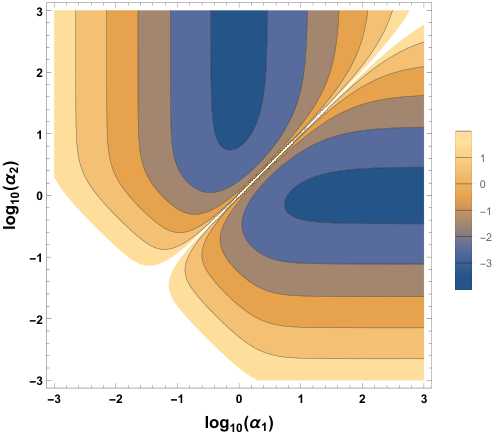
After these preliminary steps, we can discuss the uncertainties that affect the $\hat{\sigma}^{\rm SM}_{r}$, $\hat{\sigma}^{\rm int}_{r}$ and $\hat{\sigma}^{\rm BSM}_{r}$ estimators. We aim at minimizing simultaneously the uncertainties for every component. We should therefore consider the trace of the relative covariance matrix of Eq. (33). Let us first notice that choosing $\alpha_{0}=0$ gives simply $\hat{\sigma}^{\rm SM}_{r}=\hat{\sigma}^{0}_{r}$ and therefore the relative variance for $\hat{\sigma}^{\rm SM}_{r}$ is simply $\bar{V}_{r}^{\rm SM}=\bar{V}_{r}$. This choice is arguably optimal and we are left with finding optimal values for $\alpha_{1}$ and $\alpha_{2}$.

For a fixed value of $\alpha_{1}$ it turns out that $\operatorname{tr}\bar{C}_{r}(0,\alpha_{1},\alpha_{2})$ is minimized for $\alpha_{2}$ going to infinity ⁸⁸ 8 Because of the symmetry in ($\alpha_{1}$, $\alpha_{2}$) the same is also true for fixed $\alpha_{2}$ and $\alpha_{1}\to\infty$. and this runaway direction can be seen in Fig. 2. In this limit, the $\hat{\sigma}_{r}^{2}$ estimator corresponds exactly to $\hat{\sigma}^{\rm BSM}_{r}$ with relative variance equal to $\bar{V}_{r}$ and vanishing correlation with $\hat{\sigma}^{\rm SM}_{r}$. In this limit the relative covariance matrix takes the form

The trace of the relative variance matrix goes to infinity for both $\alpha_{1}\rightarrow 0,\infty$ because the linear system becomes degenerate in these limits. Studying further the behaviour of $\operatorname{tr}\bar{C}_{r}(0,\alpha_{1},\infty)$ we find out that it admits two minima for

It is a non-trivial feature that this expression is independent on $\sigma_{r}^{\rm int}$. This implies that the optimization does not depend on whether the interference is suppressed.

The behaviour of the trace of $\bar{C}_{r}(0,\alpha_{1},\alpha_{2})$ is shown in Fig. 2, where we have taken $\Lambda$ to be such that Eq. (34) is verified. One can observe from the plot that the minimum of the trace of the relative covariance matrix occurs for $\alpha_{1}=1$, $\alpha_{2}=\infty$ or vice-versa. The relative covariance matrix at the positive optimal $\alpha_{1}$ takes the following form

where

Notice that the minimal relative covariance being by definition dimensionless, it can depend on the components of the differential rate only through the combination $\bar{\sigma}_{r}/\sigma_{r}^{\rm int}$. This quantity is also the one appearing in the Cauchy-Schwartz bound of Eq. (12) that now can be rewritten as $|\sigma_{r}^{\rm int}|\leq 2\bar{\sigma}_{r}$.

Considering the two values of $\sigma_{r}^{\rm int}$ that saturate the Cauchy-Schwartz bound, the relative covariance matrix at the minimum assumes the following form

for $\sigma^{\rm int}_{r}=+2\bar{\sigma}_{r}$ and $\sigma^{\rm int}_{r}=-2\bar{\sigma}_{r}$ respectively. The relative uncertainty on the interference component is given by the square root of $(\bar{C}_{r})_{22}$. From Eq. (39) one sees that the uncertainty on the interference component is larger than the ones on $\sigma^{\rm SM}_{r}$, $\sigma^{\rm BSM}_{r}$ by at least a factor $3/\sqrt{2}$ when $\sigma^{\rm int}_{r}$ is positive. In case of a maximal negative interference, the optimal $\alpha_{1}$ corresponds in fact to a fully destructive interference, $\sigma_{r}^{1}=0$, and the expected uncertainty associated to this result is vanishing. This can be directly seen in the covariance matrix (Eq. (39), right side), which features a zero eigenvalue. This situation of a large negative interference gives the smallest uncertainties possible. In contrast, whenever the interference is suppressed, $|\sigma^{\rm int}_{r}|<2\bar{\sigma}_{r}$, the uncertainty on the interference component quickly blows up. For example, taking $\sigma^{\rm int}_{r}=\pm 0.2\bar{\sigma}_{r}$, we get $(\bar{C}_{r})_{22}\approx 175$ and $(\bar{C}_{r})_{22}\approx 130$ respectively. Our calculation provides a quantitative estimate of the difficulties that will be encountered for determining the interference component.

If one evaluates the minimal relative covariance matrix at the negative optimal $\alpha_{1}$ of Eq. (36), Eq. (39) and the subsequent expressions and discussions are valid up to a sign flip of $\sigma^{\rm int}_{r}$. Let us notice that if the sign of $\sigma^{\rm int}_{r}$ is known in advance, the sign of the optimal $\alpha_{1}$ can then be chosen so that the interference term is negative, which gives a better uncertainty on the estimation of $\sigma^{\rm int}_{r}$. But this refinement matters mostly for an interference near the Cauchy-Schwartz bound.

Finally, one may notice that the optimization is in principle different for each bin, as made clear by the $r$-dependence of the optimal point given in Eq. (36). However a simpler version of the optimization can also be obtained by using the $\alpha_{1}$ that minimizes the uncertainty on the total rates, namely $\alpha_{1}=\Lambda^{2}(\sigma^{\rm SM}/\sigma^{\rm BSM})^{1/2}$.

Let us discuss the reconstruction method in the case of $n$ effective operators. We have seen in section 3.1 that $(n+1)(n+2)/2$ simulations have to be performed to fully reconstruct the event rate $\sigma_{X}$ as function of the $\alpha_{I}$’s. In practice, it turns out it is sufficient to switch on one or two effective operators at a time in order to reconstruct all the components. Using the results of the previous section, we can provide the complete list of $(n+1)(n+2)/2$ optimized points to be used for the simulations. We have:

1. 1)

   One point with all $\alpha_{I}=0$.

2. 2)

   For every $I$, a single non-zero $\alpha_{I}$ satisfying $\alpha_{I}\gg 1$. These are $n$ points.

3. 3)

   For every $I$, a single non-zero $\alpha_{I}$ satisfying $\alpha_{I}\sim\Lambda^{2}\frac{(\sigma_{X}^{\rm SM})^{1/2}}{(\sigma^{\rm BSM}_{X,II})^{1/2}}$. These are $n$ points.

4. 4)

   For every pair $(I,J)$, a single non-zero pair $(\alpha_{I},\alpha_{J})$ satisfying $\alpha_{I,J}\gg 1$ and $\alpha_{I}\sigma^{\rm BSM}_{X,II}\sim\alpha_{J}\sigma^{\rm BSM}_{X,JJ}$. These are $n(n-1)/2$ points.

We thus end up with a system of $(n+1)(n+2)/2$ linear equations that has to be solved. A useful side effect of the optimization described in the previous subsection is that the calculation of the various components becomes more transparent. In particular, 1) provides $\sigma_{X}^{\rm SM}$ and 2) provides the $\sigma^{\rm BSM}_{X,II}$ components. 3) provides the interference terms $\sigma^{\rm int}_{X,I}$ which can be simply obtained by subtracting $\sigma_{X}^{\rm SM}+\alpha_{I}^{2}\Lambda^{-4}\sigma^{\rm BSM}_{X,II}$ from the outcome of the simulations in 3), instead of using the exact formulas of Eqs. (27). This simplification is a consequence of having used arbitrary large $\alpha_{I}$’s in 2). Similarly, 4) provides the $\sigma^{\rm BSM}_{X,IJ}$ components, which are obtained by subtracting $\alpha_{I}^{2}\sigma^{\rm BSM}_{X,II}+\alpha_{J}^{2}\sigma^{\rm BSM}_{X,JJ}$ from the outcome of the simulations in 4). An analysis similar to the one of section 3.2 shows that the uncertainty on the $\sigma^{\rm BSM}_{X,IJ}$ terms is minimized for $\alpha_{I}\sigma^{\rm BSM}_{X,II}\sim\alpha_{J}\sigma^{\rm BSM}_{X,JJ}$.

References

- (1) CMS Collaboration, S. Chatrchyan et al., Observation of a new boson at a mass of 125 GeV with the CMS experiment at the LHC, Phys.Lett. B716 (2012) 30–61, [arXiv:1207.7235].
- (2) ATLAS Collaboration, G. Aad et al., Observation of a new particle in the search for the Standard Model Higgs boson with the ATLAS detector at the LHC, Phys.Lett. B716 (2012) 1–29, [arXiv:1207.7214].
- (3) J. Ellis, V. Sanz, and T. You, The Effective Standard Model after LHC Run I, JHEP 03 (2015) 157, [arXiv:1410.7703].
- (4) T. Corbett, O. J. P. Eboli, D. Goncalves, J. Gonzalez-Fraile, T. Plehn, and M. Rauch, The Higgs Legacy of the LHC Run I, JHEP 08 (2015) 156, [arXiv:1505.05516].
- (5) A. Butter, O. J. P. Éboli, J. Gonzalez-Fraile, M. C. Gonzalez-Garcia, T. Plehn, and M. Rauch, The Gauge-Higgs Legacy of the LHC Run I, JHEP 07 (2016) 152, [arXiv:1604.03105].
- (6) S. Fichet, New likelihoods for shape analysis, Int. J. Mod. Phys. A30 (2015), no. 09 1550039, [arXiv:1407.1865].
- (7) J. Alwall, M. Herquet, F. Maltoni, O. Mattelaer, and T. Stelzer, MadGraph 5 : Going Beyond, JHEP 06 (2011) 128, [arXiv:1106.0522].
- (8) S. Fichet and G. von Gersdorff, Effective theory for neutral resonances and a statistical dissection of the ATLAS diboson excess, JHEP 12 (2015) 089, [arXiv:1508.04814].
- (9) R. Contino, A. Falkowski, F. Goertz, C. Grojean, and F. Riva, On the Validity of the Effective Field Theory Approach to SM Precision Tests, JHEP 07 (2016) 144, [arXiv:1604.06444].
- (10) A. Azatov, R. Contino, C. S. Machado, and F. Riva, Helicity Selection Rules and Non-Interference for BSM Amplitudes, arXiv:1607.05236.
- (11) B. Grzadkowski, M. Iskrzynski, M. Misiak, and J. Rosiek, Dimension-Six Terms in the Standard Model Lagrangian, JHEP 1010 (2010) 085, [arXiv:1008.4884].
- (12) G. Cowan, K. Cranmer, E. Gross, and O. Vitells, Asymptotic formulae for likelihood-based tests of new physics, Eur.Phys.J. C71 (2011) 1554, [arXiv:1007.1727].
- (13) K. Hagiwara, R. Peccei, D. Zeppenfeld, and K. Hikasa, Probing the Weak Boson Sector in e+ e- –¿ W+ W-, Nucl.Phys. B282 (1987) 253.
- (14) S. Fichet and G. von Gersdorff, Anomalous gauge couplings from composite Higgs and warped extra dimensions, JHEP03(2014)102 (2013) [arXiv:1311.6815].
- (15) CMS Collaboration, V. Khachatryan et al., Measurement of the cross section in pp collisions at 8 TeV and limits on anomalous gauge couplings, Eur. Phys. J. C76 (2016), no. 7 401, [arXiv:1507.03268].
- (16) A. Alloul, N. D. Christensen, C. Degrande, C. Duhr, and B. Fuks, FeynRules 2.0 - A complete toolbox for tree-level phenomenology, Comput. Phys. Commun. 185 (2014) 2250–2300, [arXiv:1310.1921].
- (17) T. Sjostrand, S. Mrenna, and P. Z. Skands, PYTHIA 6.4 Physics and Manual, JHEP 05 (2006) 026, [hep-ph/0603175].
- (18) A. Falkowski, M. Gonzalez-Alonso, A. Greljo, D. Marzocca, and M. Son, Anomalous Triple Gauge Couplings in the Effective Field Theory Approach at the LHC, arXiv:1609.06312.
- (19) S. Fichet, Taming systematic uncertainties at the LHC with the central limit theorem, Nucl. Phys. B911 (2016) 623–637, [arXiv:1603.03061].
- (20) L. Brenner, N. Belyaev, V. Bortolotto, C. D. Burgard, M. Duehrssen-Debling, K. M. Ecker, S. Gadatsch, D. S. Gray, A. Kaluza, K. Koeneke, R. Konoplich, S. Kortner, K. Prokofiev, C. Schmitt, and W. Verkerke, A morphing technique for signal modelling in a multidimensional space of coupling parameters, .
- (21) A morphing technique for signal modelling in a multidimensional space of coupling parameters, Tech. Rep. ATL-PHYS-PUB-2015-047, CERN, Geneva, Nov, 2015.