跳到论文正文
W Papers独立论文阅读器 arXiv:1611.01129 论文正文 计算阅读时间 · 0%
引用这篇论文根据当前论文元数据生成,正式投稿前建议核对。


License: CC BY-SA 4.0
arXiv:1611.01129v2 [stat.ME] 27 Nov 2018

Cross: Efficient Low-rank Tensor Completion

Anru Zhang?? abel=u1    url]www.stat.wisc.edu/∼\scriptstyle\simanruzhang/

The completion of tensors, or high-order arrays, attracts significant attention in recent research. Current literature on tensor completion primarily focuses on recovery from a set of uniformly randomly measured entries, and the required number of measurements to achieve recovery is not guaranteed to be optimal. In addition, the implementation of some previous methods is NP-hard. In this article, we propose a framework for low-rank tensor completion via a novel tensor measurement scheme we name Cross. The proposed procedure is efficient and easy to implement. In particular, we show that a third order tensor of Tucker rank-(r1,r2,r3)(r_{1},r_{2},r_{3}) in p1p_{1}-by-p2p_{2}-by-p3p_{3} dimensional space can be recovered from as few as r1​r2​r3+r1​(p1−r1)+r2​(p2−r2)+r3​(p3−r3)r_{1}r_{2}r_{3}+r_{1}(p_{1}-r_{1})+r_{2}(p_{2}-r_{2})+r_{3}(p_{3}-r_{3}) noiseless measurements, which matches the sample complexity lower-bound. In the case of noisy measurements, we also develop a theoretical upper bound and the matching minimax lower bound for recovery error over certain classes of low-rank tensors for the proposed procedure. The results can be further extended to fourth or higher-order tensors. Simulation studies show that the method performs well under a variety of settings. Finally, the procedure is illustrated through a real dataset in neuroimaging.

University of Wisconsin-Madison

1 Introduction

Tensors, or high-order arrays, commonly arise in a wide range of applications, including neuroimaging (Zhou et al., 2013; Li et al., 2013; Guhaniyogi et al., 2017; Li and Zhang, 2016; Sun and Li, 2016), recommender systems (Karatzoglou et al., 2010; Rendle and Schmidt-Thieme, 2010; Sun et al., 2015), hyperspectral image compression (Li and Li, 2010), multi-energy computed tomography (Semerci et al., 2014; Li et al., 2014), computer vision (Liu et al., 2013), 3D light field displays (Wetzstein et al., 2012) and scientific computation (Oseledets and Tyrtyshnikov, 2009). With the revolutionary development of modern technologies, the rapid increase in data dimension, memory and time expenses outgrows the power of computing devices, which makes it difficult to work directly on the complete datasets and models. For example, a tensor of dimension 10410^{4}-by-10410^{4}-by-10410^{4} would be difficult to upload into the Random Access Memory (RAM) of a typical computer, making it hard to directly perform operations that involves all entries of the tensor. In order to conduct various statistical tensor data analyses, such as SVD or PCA (Richard and Montanari, 2014; Zhang and Xia, 2018) and Monte-Carlo algorithms for computations on large tensors (Guhaniyogi et al., 2017; Johndrow et al., 2017) when limited computation power is available, a fast and sufficient tensor compression is essential. To this end, a natural idea is to sample a small portion of entries from the original tensor dataset that preserves the important structural information and allows efficient recovery. By storing these entries to RAM, the follow-up tensor data analysis can be highly facilitated.

Tensor completion, whose central goal is to recover low-rank tensors based on limited numbers of measurable entries, is a plausible idea for compression and decompression of high-dimensional low-rank tensors. Such problems have been central and well-studied for order-2 tensors (i.e. matrices) in the fields of high-dimensional statistics and machine learning for the last decade. A large body of matrix completion literatures focused on the scenario of uniformly randomly sampled observations (Keshavan et al., 2009; Candès and Tao, 2010; Koltchinskii et al., 2011; Rohde et al., 2011; Negahban and Wainwright, 2011; Agarwal et al., 2012), but there exists another line of works where the observations are collected by other means, such as deterministically sampling patterns (Pimentel-Alarcón et al., 2016), column-subset-selection (Rudelson and Vershynin, 2007; Krishnamurthy and Singh, 2013; Wang and Singh, 2015; Cai et al., 2016) and general sampling distributions (Klopp, 2014). There are efficient procedures for matrix completion with strong theoretical guarantees. For example, for a p1p_{1}-by-p2p_{2} matrix of rank-rr, whenever roughly O⁡(r⁡(p1+p2)​polylog​(p1+p2))O(r(p_{1}+p_{2})\text{polylog}(p_{1}+p_{2})) uniformly randomly selected entries are observed, one can achieve nice recovery with high probability using convex algorithms such as matrix nuclear norm minimization (Candès and Tao, 2010; Recht, 2011) and max-norm minimization (Srebro and Shraibman, 2005; Cai and Zhou, 2016). For matrix completion, the required number of measurements nearly matches the degrees of freedom, O⁡((p1+p2)​r)O((p_{1}+p_{2})r), for p1p_{1}-by-p2p_{2} matrices of rank-rr.

Although significant progress has been made for matrix completion, similar problems for order-3 or higher tensors are far more difficult. There have been some recent literature, including Gandy et al. (2011); Kressner et al. (2014); Yuan and Zhang (2014); Mu et al. (2014); Bhojanapalli and Sanghavi (2015); Shah et al. (2015); Barak and Moitra (2016); Yuan and Zhang (2016), that studied tensor completion based on similar formulations. To be specific, let 𝐗∈ℝp1×p2×p3{\mathbf{X}}\in\mathbb{R}^{p_{1}\times p_{2}\times p_{3}} be an order-33 low-rank tensor, and 𝛀\boldsymbol{\Omega} be a subset of [1:p1]×[1:p2]×[1:p3][1:p_{1}]\times[1:p_{2}]\times[1:p_{3}]. The goal of tensor completion is to recover 𝐗{\mathbf{X}} based on the observable entries indexed by 𝛀\boldsymbol{\Omega}. Most of the previous literature focuses on the setting where the indices of the observable entries are uniformly randomly selected. For example, Gandy et al. (2011); Liu et al. (2013) proposed the matricization nuclear norm minimization, which requires O⁡(r​p2​polylog​(p))O(rp^{2}\text{polylog}(p)) observations to recover order-3 tensors of dimension pp-by-pp-by-pp and Tucker rank-(r,r,r)(r,r,r). Later, Jain and Oh (2014); Bhojanapalli and Sanghavi (2015) considered an alternative minimization method for completion of low-rank tensors with CP decomposition and orthogonal factors. Yuan and Zhang (2014); Yuan and Zhang (2016) proposed the tensor nuclear norm minimization algorithm for tensor completion with noiseless observations and further proved that their proposed method has guaranteed performance for pp-by-pp-by-pp tensors of Tucker rank-(r,r,r)(r,r,r) with high probability when |𝛀|≥O⁡((r1/2​p3/2+r2​p)​polylog​(p))|\boldsymbol{\Omega}|\geq O((r^{1/2}p^{3/2}+r^{2}p)\text{polylog}(p)). However, it is unclear whether the required number of measurements in this literature could be further improved or not. In addition, some of these proposed procedures, such as tensor matrix nuclear norm minimization, are proved to be computationally NP-hard, making them very difficult to apply in real problems. Recently, Barak and Moitra (2016) further showed that the completion of pp-by-pp-by-pp low-rank tensors is computationally infeasible when only O⁡(p3/2)O(p^{3/2}) uniform random entries are observable, unless a more efficient algorithm exists for boolean satisfiability problem.

The central goal of this paper is to address the following question: is it possible to perform efficient low-rank tensor completion with a small number of observable entries? If so, what is the sample complexity, i.e., the minimal number of entries one needs to observe, so that there exist fast algorithms for tensor completion with guaranteed performance? This problem is important to statistical learning theory and is inevitable in many high-dimensional tensor data analyses. Given the previous discussions, to sample entries uniformly at random may not be an optimal strategy to achieve the central goal. Instead, we propose a novel tensor measurement scheme and the corresponding efficient low-rank tensor completion algorithm. We name our methods Cross Tensor Measurement Scheme because the measurement set is in the shape of a high-dimensional cross contained in the tensor. We show that one can recover an unknown, Tucker rank-(r1,r2,r3)(r_{1},r_{2},r_{3}), and p1p_{1}-by-p2p_{2}-by-p3p_{3} tensor 𝐗{\mathbf{X}} with

|𝛀|=r1​r2​r3+r1​(p1−r1)+r2​(p2−r2)+r3​(p3−r3)|\boldsymbol{\Omega}|=r_{1}r_{2}r_{3}+r_{1}(p_{1}-r_{1})+r_{2}(p_{2}-r_{2})+r_{3}(p_{3}-r_{3})

noiseless Cross tensor measurements. This outperforms the previous methods in literature, and matches the degrees of freedom for all rank-(r1,r2,r3)(r_{1},r_{2},r_{3}) tensors of dimensions p1p_{1}-by-p2p_{2}-by-p3p_{3}. To the best of our knowledge, we are among the first to achieve this optimal rate. We also develop the corresponding recovery method for more general cases where measurements are taken with noise. The central idea is to transform the observable matricizations by singular value decomposition and perform the adaptive trimming scheme to denoise each block.

To illustrate the properties of the proposed procedure, both theoretical analyses and simulation studies are provided. We derive upper and lower bound results to show that the proposed recovery procedure can accommodate different levels of noise and achieve the optimal rate of convergence for a large class of low-rank tensors. Although the exact low-rank assumption is used in the theoretical analysis, some simulation settings show that such an assumption is not really necessary in practice, as long as the singular values of each matricization of the original tensor decays sufficiently.

It is worth emphasizing that because the proposed algorithms only involve basic matrix operations such as matrix multiplication and singular value decomposition, it is tuning-free in many general situations and can be implemented efficiently to handle large scale problems. In fact, our simulation study shows that the recovery of a 500-by-500-by-500 tensor can be done stably within, on average, 10 seconds.

We also apply the proposed procedure to a 3-d MRI imaging dataset that comes from a study on Attention-deficit/hyperactivity disorder (ADHD). We show that with a limited number of Cross tensor measurements and the corresponding tensor completion algorithm, one can estimate the underlying low-rank structure of 3-d images as well as if one observes all entries of the image.

This work also relates to some previous results other than tensor completion in the literature. Mahoney et al. (2008) considered the tensor CUR decomposition, which aims to represent the tensor as the product of a sub-tensor and two matrices. However, simply applying their work cannot lead to optimal results in tensor completion since treating tensors as matrix slices would lose useful structures of tensors. Krishnamurthy and Singh (2013) proposed a sequential tensor completion algorithm under adaptive samplings. Their result requires O⁡(p​r2.5​log⁡(r))O(pr^{2.5}\log(r)) number of entries for pp-by-pp-by-pp order-3 tensors under the more restrictive CP rank-rr condition, which is much larger than that of our method. Rauhut et al. (2016) considered a tensor recovery setting where each observation is a general linear projections of the original tensor. However, their theoretical analysis heavily relies on a conjecture that is difficult to check. Oseledets et al. (2008) provided an existence proof for rank-rr Tucker-like approximations for pp-by-pp-by-pp tensors with O⁡(r3+p​r)O(r^{3}+pr) parameters. Caiafa and Cichocki (2010) introduced representations for p1p_{1}-by-p2p_{2}-by-p3p_{3} Tucker rank-(r,r,r)(r,r,r) tensors based on r3+r⁡(p1+p2+p3)r^{3}+r(p_{1}+p_{2}+p_{3}) selected entries. In Caiafa and Cichocki (2015), they further introduced a multi-way projection scheme for stable, robust, and fast low-rank tensor reconstruction, which requires O⁡(p​r2)O(pr^{2}) measurements and some tuning parameters, such as the rank of the tensor, for implementation. To the extent of our knowledge, we are among the first to develop the tensor completion scheme that is efficient, easy to implement, tuning-free, and allows exact tensor completion in the noiseless setting and achieves optimal estimation error in the noisy setting under the minimal sample size.

The rest of the paper is organized as follows. After an introduction to the notations and preliminaries in Section 2.1, we present the Cross tensor measurement scheme in Section 2.2. Based on the proposed measurement scheme, the tensor completion algorithms for both noiseless and noisy case are introduced in Sections 2.3 and 2.4 respectively. We further analyze the theoretical performance of the proposed algorithms in Section 3. The numerical performance of algorithms are investigated in a variety of simulation studies in Section 4. We then apply the proposed procedure to a real dataset of brain MRI imaging in Section 5. In Section 6, we briefly discuss the extensions of main results. The proofs of the main results are finally collected in the supplement materials.

2 Cross Tensor Measurements & Completion: Methodology

2.1 Basic Notations and Preliminaries

We start with basic notations and results that will be used throughout the paper. The upper case letters, e.g., X,Y,ZX,Y,Z, are generally used to represent matrices. For X∈ℝp1×p2X\in\mathbb{R}^{p_{1}\times p_{2}}, the singular value decomposition can be written as X=U​Σ​V⊤X=U\Sigma V^{\top}. Suppose diag⁡(Σ)=(σ1​(X),…,σmin⁡{p1,p2}​(X)){\rm diag}(\Sigma)=(\sigma_{1}(X),\ldots,\sigma_{\min\{p_{1},p_{2}\}}(X)), then σ1​(X)≥σ2​(X)≥…≥σmin⁡{p1,p2}​(X)≥0\sigma_{1}(X)\geq\sigma_{2}(X)\geq\ldots\geq\sigma_{\min\{p_{1},p_{2}\}}(X)\geq 0 are the singular values of XX. Especially, we note σmin​(X)=σmin⁡{p1,p2}​(X)\sigma_{\min}(X)=\sigma_{\min\{p_{1},p_{2}\}}(X) and σmax​(X)=σ1​(X)\sigma_{\max}(X)=\sigma_{1}(X) as the smallest and largest singular value of XX. Additionally, the matrix spectral norm and Frobenius norm are denoted as ‖X‖=maxu∈ℝp2⁡‖X​u‖2‖u‖2\|X\|=\max_{u\in\mathbb{R}^{p_{2}}}\frac{\|Xu\|_{2}}{\|u\|_{2}} and ‖X‖F=∑i=1p1∑j=1p2Xi​j2=∑i=1min⁡{p1,p2}σi2​(X)\|X\|_{F}=\sqrt{\sum_{i=1}^{p_{1}}\sum_{j=1}^{p_{2}}X_{ij}^{2}}=\sqrt{\sum_{i=1}^{\min\{p_{1},p_{2}\}}\sigma_{i}^{2}(X)}, respectively. We denote ℙX∈ℝp1×p1\mathbb{P}_{X}\in\mathbb{R}^{p_{1}\times p_{1}} as the projection operator onto the column space of XX. Specifically, ℙX=X​(X⊤​X)†​X⊤=X​X†\mathbb{P}_{X}=X(X^{\top}X)^{\dagger}X^{\top}=XX^{\dagger}. Here (⋅)†(\cdot)^{\dagger} is the Moore-Penrose pseudo-inverse. Let 𝕆p,r\mathbb{O}_{p,r} be the set of all pp-by-rr orthogonal columns, i.e., 𝕆p,r={V∈ℝp×r:V⊤​V=Ir}\mathbb{O}_{p,r}=\{V\in\mathbb{R}^{p\times r}:V^{\top}V=I_{r}\}, where IrI_{r} represents the identity matrix of dimension rr.

We use bold upper case letters, e.g., 𝐗,𝐘,𝐙{\mathbf{X}},{\mathbf{Y}},{\mathbf{Z}} to denote tensors. If 𝐗∈ℝp1×p2×p3{\mathbf{X}}\in\mathbb{R}^{p_{1}\times p_{2}\times p_{3}}, Et∈ℝmt×ptE_{t}\in\mathbb{R}^{m_{t}\times p_{t}}, t=1,2,3t=1,2,3. The mode products (tensor-matrix product) is defined as

𝐗×1E1∈ℝm1×p2×p3,(𝐗×1E1)i​j​k=∑s=1p1E1,i​s​𝐗s​j​k,{\mathbf{X}}\times_{1}E_{1}\in\mathbb{R}^{m_{1}\times p_{2}\times p_{3}},\quad\left({\mathbf{X}}\times_{1}E_{1}\right)_{ijk}=\sum_{s=1}^{p_{1}}E_{1,is}{\mathbf{X}}_{sjk},

where i∈[1:m1],j∈[1:p2],k∈[1:p3]i\in[1:m_{1}],j\in[1:p_{2}],k\in[1:p_{3}]. The mode-2 product 𝐗×2E2{\mathbf{X}}\times_{2}E_{2} and mode-3 product 𝐗×3E3{\mathbf{X}}\times_{3}E_{3} can be defined similarly. Interestingly, the products along different modes satisfy the commutative law, e.g., 𝐗×tEt×sEs=𝐗×sEs×tEt{\mathbf{X}}\times_{t}E_{t}\times_{s}E_{s}={\mathbf{X}}\times_{s}E_{s}\times_{t}E_{t} if s≠ts\neq t. The matricization (or unfolding, flattening in literature), ℳt​(𝐗)\mathcal{M}_{t}({\mathbf{X}}), maps a tensor 𝐗∈ℝp1×p2×p3{\mathbf{X}}\in\mathbb{R}^{p_{1}\times p_{2}\times p_{3}} into a matrix ℳt​(𝐗)∈ℝpt×∏s≠tps\mathcal{M}_{t}({\mathbf{X}})\in\mathbb{R}^{p_{t}\times\prod_{s\neq t}p_{s}}, so that for any i∈{1,⋯,p1},j∈{1,⋯,p2},k∈{1,⋯,p3}i\in\{1,\cdots,p_{1}\},j\in\{1,\cdots,p_{2}\},k\in\{1,\cdots,p_{3}\},

𝐗i​j​k=(ℳ1​(𝐗))[i,(j+p2​(k−1))]=(ℳ2​(𝐗))[j,(k+p3​(i−1))]=(ℳ3​(𝐗))[k,(i+p1​(j−1))].\begin{split}{\mathbf{X}}_{ijk}=(\mathcal{M}_{1}({\mathbf{X}}))_{[i,(j+p_{2}(k-1))]}=(\mathcal{M}_{2}({\mathbf{X}}))_{[j,(k+p_{3}(i-1))]}=(\mathcal{M}_{3}({\mathbf{X}}))_{[k,(i+p_{1}(j-1))]}.\end{split}

The tensor Hilbert Schmidt norm and tensor spectral norm, which are defined as

‖𝐗‖HS=∑i=1p1∑j=1p2∑k=1p3𝐗i​j​k2,‖𝐗‖op=maxu∈ℝp1,v∈ℝp2,w∈ℝp3⁡𝐗×1u×2v×3w‖u‖2​‖v‖2​‖w‖2,\|{\mathbf{X}}\|_{\rm HS}=\sqrt{\sum_{i=1}^{p_{1}}\sum_{j=1}^{p_{2}}\sum_{k=1}^{p_{3}}{\mathbf{X}}_{ijk}^{2}},\quad\left\|{\mathbf{X}}\right\|_{\rm op}=\max_{u\in\mathbb{R}^{p_{1}},v\in\mathbb{R}^{p_{2}},w\in\mathbb{R}^{p_{3}}}\frac{{\mathbf{X}}\times_{1}u\times_{2}v\times_{3}w}{\|u\|_{2}\|v\|_{2}\|w\|_{2}},

will be intensively used in this paper. It is also noteworthy that the general calculation of the tensor operator norm is NP-hard (Hillar and Lim, 2013). Unlike matrices, there is no universal definition of rank for third or higher order tensors. Standing out from various definitions, the Tucker rank (Tucker, 1966) has been widely utilized in literature, and its definition is closely associated with the following Tucker decomposition: for 𝐗∈ℝp1×p2×p3{\mathbf{X}}\in\mathbb{R}^{p_{1}\times p_{2}\times p_{3}},

𝐗=𝐒×1U1×2U2×3U3,or equivalently𝐗i​j​k=∑i′​j′​k′si′​j′​k′U1,i​i′U2,j​j′U3,k​k′.{\mathbf{X}}={\mathbf{S}}\times_{1}U_{1}\times_{2}U_{2}\times_{3}U_{3},\quad\text{or equivalently}\quad{\mathbf{X}}_{ijk}=\sum_{i^{\prime}j^{\prime}k^{\prime}}s_{i^{\prime}j^{\prime}k^{\prime}}U_{1,ii^{\prime}}U_{2,jj^{\prime}}U_{3,kk^{\prime}}. (2.1)

Here 𝐒∈ℝr1×r2×r3{\mathbf{S}}\in\mathbb{R}^{r_{1}\times r_{2}\times r_{3}} is referred to as the core tensor, Uk∈𝕆pk,rkU_{k}\in\mathbb{O}_{p_{k},r_{k}}. The minimum number of triplets (r1,r2,r3)(r_{1},r_{2},r_{3}) are defined as the Tucker rank of 𝐗{\mathbf{X}} which we denote as rank⁡(𝐗)=(r1,r2,r3){\rm rank}({\mathbf{X}})=(r_{1},r_{2},r_{3}). The Tucker rank can be calculated easily by the rank of each matricization: rt=rank⁡(ℳt​(𝐗))r_{t}={\rm rank}(\mathcal{M}_{t}({\mathbf{X}})). It is also easy to prove that the triplet (r1,r2,r3)(r_{1},r_{2},r_{3}) satisfies rt≤pt,max2⁡{r1,r2,r3}≤r1​r2​r3r_{t}\leq p_{t},\max^{2}\{r_{1},r_{2},r_{3}\}\leq r_{1}r_{2}r_{3}. For a more detailed survey of tensor decomposition, readers are referred to Kolda and Bader (2009).

We also use the following symbols to represent sub-arrays. For any subsets Ω1,Ω2\Omega_{1},\Omega_{2}, etc., we use X[Ω1,Ω2]X_{[\Omega_{1},\Omega_{2}]} to represent the sub-matrix of XX with row indices Ω1\Omega_{1} and column indices Ω2\Omega_{2}. The sub-tensors are denoted similarly: 𝐗[Ω1,Ω2,Ω3]{\mathbf{X}}_{[\Omega_{1},\Omega_{2},\Omega_{3}]} represents the tensors with mode-tt indices in Ωt\Omega_{t} for t=1,2,3t=1,2,3. For better presentation, we use bracket to represent index sets. Particularly for any integers a≤ba\leq b, let [a:b]={a,…,b}[a:b]=\{a,\ldots,b\} and let “:” alone represent the whole index set. Thus, U[:,1:r]U_{[:,1:r]} represents the first rr columns of UU; 𝐗[Ω1,Ω2,:]{\mathbf{X}}_{[\Omega_{1},\Omega_{2},:]} represents the sub-tensor of 𝐗{\mathbf{X}} with mode-1 indices Ω1\Omega_{1}, mode-2 indices Ω2\Omega_{2} and all mode-3 indices.

Now we establish the lower bound for the minimum number of measurements for Tucker low-rank tensor completion based on counting the degrees of freedom.

Proposition 1 (Degrees of freedom for rank-(r1,r2,r3)(r_{1},r_{2},r_{3}) tensors in ℝp1×p2×p3\mathbb{R}^{p_{1}\times p_{2}\times p_{3}}).

Assume that r1≤p1,r2≤p2,r3≤p3r_{1}\leq p_{1},r_{2}\leq p_{2},r_{3}\leq p_{3}, max2⁡{r1,r2,r3}≤r1​r2​r3\max^{2}\{r_{1},r_{2},r_{3}\}\leq r_{1}r_{2}r_{3}, then the degrees of freedom of all rank-(r1,r2,r3)(r_{1},r_{2},r_{3}) tensors in ℝp1×p2×p3\mathbb{R}^{p_{1}\times p_{2}\times p_{3}} is

r1​r2​r3+(p1−r1)​r1+(p2−r2)​r2+(p3−r3)​r3.r_{1}r_{2}r_{3}+(p_{1}-r_{1})r_{1}+(p_{2}-r_{2})r_{2}+(p_{3}-r_{3})r_{3}.
Remark 1.

Beyond order-3 tensors, we can show the degrees of freedom for rank-(r1,…,rd)(r_{1},\ldots,r_{d}) order-dd tensors in ℝp1×⋯×pd\mathbb{R}^{p_{1}\times\cdots\times p_{d}} is ∏t=1drt+∑t=1drt​(pt−rt)\prod_{t=1}^{d}r_{t}+\sum_{t=1}^{d}r_{t}(p_{t}-r_{t}) similarly.

Proposition 1 provides a lower bound and the benchmark for the number of measurements to guarantee low-rank tensor completion, i.e., r1​r2​r3+∑t=13rt​(pt−rt)r_{1}r_{2}r_{3}+\sum_{t=1}^{3}r_{t}(p_{t}-r_{t}). Since the previous methods are not guaranteed to achieve this lower bound, we focus on developing the first measurement scheme that can both work efficiently and reach this benchmark.

2.2 Cross Tensor Measurements

In this section, we propose a novel Cross tensor measurement scheme. Suppose the targeting unknown tensor 𝐗{\mathbf{X}} is of p1p_{1}-by-p2p_{2}-by-p3p_{3}, we let

Ω1⊆[1:p1],Ω2⊆[1:p2],Ω3⊆[1:p3],|Ωt|=mt,t=1,2,3;Ξ1⊆Ω2×Ω3,Ξ2⊆Ω3×Ω1,Ξ3⊆Ω1×Ω2,|Ξt|=gt,t=1,2,3.\begin{split}&\Omega_{1}\subseteq[1:p_{1}],\quad\Omega_{2}\subseteq[1:p_{2}],\quad\Omega_{3}\subseteq[1:p_{3}],\quad|\Omega_{t}|=m_{t},\quad t=1,2,3;\\ &\Xi_{1}\subseteq\Omega_{2}\times\Omega_{3},\quad\Xi_{2}\subseteq\Omega_{3}\times\Omega_{1},\quad\Xi_{3}\subseteq\Omega_{1}\times\Omega_{2},\quad|\Xi_{t}|=g_{t},\quad t=1,2,3.\end{split} (2.2)

Then we measure the entries of 𝐗{\mathbf{X}} using the following indices set

𝛀=(Ω1×Ω2×Ω3)∪([1:p1]×Ξ1)∪([1:p2]×Ξ2)∪([1:p3]×Ξ3),\boldsymbol{\Omega}=\left(\Omega_{1}\times\Omega_{2}\times\Omega_{3}\right)\cup\left([1:p_{1}]\times\Xi_{1}\right)\cup\left([1:p_{2}]\times\Xi_{2}\right)\cup\left([1:p_{3}]\times\Xi_{3}\right), (2.3)

where

Ω1×Ω2×Ω3={(i,j,k):i∈Ω1,j∈Ω2,k∈Ω3}are body measurements;[1:p1]×Ξ1={(i,j,k):i∈[1:p1],(j,k)∈Ξ1}[1:p2]×Ξ2={(i,j,k):j∈[1:p2],(k,i)∈Ξ2}[1:p3]×Ξ3={(i,j,k):k∈[1:p3],(i,j)∈Ξ3}}arearm measurements.\begin{split}\Omega_{1}\times\Omega_{2}\times\Omega_{3}=\left\{(i,j,k):i\in\Omega_{1},j\in\Omega_{2},k\in\Omega_{3}\right\}\quad&\text{are \emph{body measurements;}}\\ \left.\begin{array}[]{ll}~[1:p_{1}]\times\Xi_{1}=\left\{(i,j,k):i\in[1:p_{1}],(j,k)\in\Xi_{1}\right\}\\ ~[1:p_{2}]\times\Xi_{2}=\left\{(i,j,k):j\in[1:p_{2}],(k,i)\in\Xi_{2}\right\}\\ ~[1:p_{3}]\times\Xi_{3}=\left\{(i,j,k):k\in[1:p_{3}],(i,j)\in\Xi_{3}\right\}\\ \end{array}\right\}\quad&\text{are\emph{arm measurements}.}\end{split} (2.4)

Meanwhile, the intersections among body and arm measurements, which we refer to as joint measurements, also play important roles in our analysis:

Ω1×Ξ1=(Ω1×Ω2×Ω3)∩([1:p1]×Ξ1)={(i,j,k):i∈Ω1,(j,k)∈Ξ1},Ω2×Ξ2=(Ω1×Ω2×Ω3)∩([1:p2]×Ξ2)={(i,j,k):j∈Ω2,(k,i)∈Ξ2},Ω3×Ξ3=(Ω1×Ω2×Ω3)∩([1:p3]×Ξ3)={(i,j,k):k∈Ω3,(i,j)∈Ξ3}.\begin{split}&\Omega_{1}\times\Xi_{1}=\left(\Omega_{1}\times\Omega_{2}\times\Omega_{3}\right)\cap\left([1:p_{1}]\times\Xi_{1}\right)=\{(i,j,k):i\in\Omega_{1},(j,k)\in\Xi_{1}\},\\ &\Omega_{2}\times\Xi_{2}=\left(\Omega_{1}\times\Omega_{2}\times\Omega_{3}\right)\cap\left([1:p_{2}]\times\Xi_{2}\right)=\{(i,j,k):j\in\Omega_{2},(k,i)\in\Xi_{2}\},\\ &\Omega_{3}\times\Xi_{3}=\left(\Omega_{1}\times\Omega_{2}\times\Omega_{3}\right)\cap\left([1:p_{3}]\times\Xi_{3}\right)=\{(i,j,k):k\in\Omega_{3},(i,j)\in\Xi_{3}\}.\end{split} (2.5)

A pictorial illustration of the body, arm and joint measurements is provided in Figure 1. Since the measurements are generally cross-shaped, we refer to 𝛀\boldsymbol{\Omega} as the Cross Tensor Measurement Scheme. It is easy to see that the total number of measurements for the proposed scheme is m1​m2​m3+g1​(p1−m1)+g2​(p2−m2)+g3​(p3−m3)m_{1}m_{2}m_{3}+g_{1}(p_{1}-m_{1})+g_{2}(p_{2}-m_{2})+g_{3}(p_{3}-m_{3}) and the sampling ratio is

#​Observable samples#​All parameters=m1​m2​m3+∑t=13gt​(pt−mt)p1​p2​p3.\frac{\#\text{Observable samples}}{\#\text{All parameters}}=\frac{m_{1}m_{2}m_{3}+\sum_{t=1}^{3}g_{t}(p_{t}-m_{t})}{p_{1}p_{2}p_{3}}. (2.6)

Based on these measurements, we focus on the following model,

𝐘𝛀=𝐗𝛀+𝐙𝛀,i.e.Yi​j​k=Xi​j​k+Zi​j​k,(i,j,k)∈𝛀,{\mathbf{Y}}_{\boldsymbol{\Omega}}={\mathbf{X}}_{\boldsymbol{\Omega}}+{\mathbf{Z}}_{\boldsymbol{\Omega}},\quad\text{i.e.}\quad Y_{ijk}=X_{ijk}+Z_{ijk},\quad(i,j,k)\in\boldsymbol{\Omega}, (2.7)

where 𝐗,𝐘{\mathbf{X}},{\mathbf{Y}} and 𝐙{\mathbf{Z}} correspond to the original tensor, observed values and unknown noise term, respectively.


Refer to caption
(a) Ωt,Ξt\Omega_{t},\Xi_{t} illustration
Refer to caption
(b) All measurements
Refer to caption
(c) Body measurements 𝐘[Ω1,Ω2​Ω3]{\mathbf{Y}}_{[\Omega_{1},\Omega_{2}\Omega_{3}]}
Refer to caption
(d) Arm measurements 𝐘Ξ1{\mathbf{Y}}_{\Xi_{1}}
Refer to caption
(e) Arm measurements 𝐘Ξ2{\mathbf{Y}}_{\Xi_{2}}
Refer to caption
(f) Arm measurements 𝐘Ξ3{\mathbf{Y}}_{\Xi_{3}}
Refer to caption
(g) Joint measurements 𝐘Ω1×Ξ1{\mathbf{Y}}_{\Omega_{1}\times\Xi_{1}}
Refer to caption
(h) Joint measurements 𝐘Ω2×Ξ2{\mathbf{Y}}_{\Omega_{2}\times\Xi_{2}}
Refer to caption
(i) Joint measurements 𝐘Ω3×Ξ3{\mathbf{Y}}_{\Omega_{3}\times\Xi_{3}}
Fig 1: Illustrative example for Cross Tensor Measurements Scheme. For better illustration here we assume Ωt=[1:mt]\Omega_{t}=[1:m_{t}], p1=p2=p3=10,m1=m2=m3=g1=g2=g3=4p_{1}=p_{2}=p_{3}=10,m_{1}=m_{2}=m_{3}=g_{1}=g_{2}=g_{3}=4.

2.3 Recovery Algorithm – Noiseless Case

When 𝐗{\mathbf{X}} is exactly low-rank and the observations are noiseless, i.e. 𝐘i​j​k=𝐗i​j​k{\mathbf{Y}}_{ijk}={\mathbf{X}}_{ijk}, we can recover 𝐗{\mathbf{X}} with the following algorithm. We first construct the arm matricizations, joint matricizations and body matricizations based on (2.4) and (2.5),

YΞt=ℳt(𝐘[1:pt]×Ξt)∈ℝpt×gt,\displaystyle Y_{\Xi_{t}}=\mathcal{M}_{t}({\mathbf{Y}}_{[1:p_{t}]\times\Xi_{t}})\in\mathbb{R}^{p_{t}\times g_{t}},\quad (Arm matricizations) (2.8)
Yt,Ω=ℳt​(𝐘[Ω1,Ω2,Ω3])∈ℝmt×∏s≠tms,\displaystyle Y_{t,\Omega}=\mathcal{M}_{t}({\mathbf{Y}}_{[\Omega_{1},\Omega_{2},\Omega_{3}]})\in\mathbb{R}^{m_{t}\times\prod_{s\neq t}m_{s}},\quad (Body matricizations) (2.9)
YΩt×Ξt=ℳt​(𝐘Ωt×Ξt)∈ℝmt×gt.\displaystyle Y_{\Omega_{t}\times\Xi_{t}}=\mathcal{M}_{t}({\mathbf{Y}}_{\Omega_{t}\times\Xi_{t}})\in\mathbb{R}^{m_{t}\times g_{t}}.\quad (Joint matricizations) (2.10)

In the noiseless setting, we propose the following formula to complete 𝐗{\mathbf{X}}:

𝐗^=𝐘[Ω1,Ω2,Ω3]×1R1×2R2×3R3,\hat{{\mathbf{X}}}={\mathbf{Y}}_{[\Omega_{1},\Omega_{2},\Omega_{3}]}\times_{1}R_{1}\times_{2}R_{2}\times_{3}R_{3}, (2.11)
whereRt=YΞt​YΩt×Ξt†∈ℝpt×mt,t=1,2,3.\text{where}\quad R_{t}=Y_{\Xi_{t}}Y_{\Omega_{t}\times\Xi_{t}}^{\dagger}\in\mathbb{R}^{p_{t}\times m_{t}},\quad t=1,2,3. (2.12)

The procedure is summarized in Algorithm 1. The theoretical guarantee for this proposed algorithm is provided in Theorem 1.

Algorithm 1 Cross: Tensor Completion with Noiseless Observations
1: Input: noiseless observations 𝐘i​j​k{\mathbf{Y}}_{ijk}, (i,j,k)∈𝛀(i,j,k)\in\boldsymbol{\Omega} from (2.3).
2: Construct YΞ1,YΞ2,XΞ3,YΩ1×Ξ1,YΩ2×Ξ2,YΩ3×Ξ3Y_{\Xi_{1}},Y_{\Xi_{2}},X_{\Xi_{3}},Y_{\Omega_{1}\times\Xi_{1}},Y_{\Omega_{2}\times\Xi_{2}},Y_{\Omega_{3}\times\Xi_{3}} as (2.8).
3: Calculate
R1=YΞ1​YΩ1×Ξ1†∈ℝp1×m1,R2=YΞ2​YΩ2×Ξ2†∈ℝp2×m2,R3=YΞ3​YΩ3×Ξ3†∈ℝp3×m3.R_{1}=Y_{\Xi_{1}}Y_{\Omega_{1}\times\Xi_{1}}^{\dagger}\in\mathbb{R}^{p_{1}\times m_{1}},~~R_{2}=Y_{\Xi_{2}}Y_{\Omega_{2}\times\Xi_{2}}^{\dagger}\in\mathbb{R}^{p_{2}\times m_{2}},~~R_{3}=Y_{\Xi_{3}}Y_{\Omega_{3}\times\Xi_{3}}^{\dagger}\in\mathbb{R}^{p_{3}\times m_{3}}.
4: Calculate the final estimator
𝐗^=𝐘[Ω1,Ω2,Ω3]×1R1×2R2×3R3.\hat{{\mathbf{X}}}={\mathbf{Y}}_{[\Omega_{1},\Omega_{2},\Omega_{3}]}\times_{1}R_{1}\times_{2}R_{2}\times_{3}R_{3}.
Theorem 1 (Exact recovery in noiseless setting).

Suppose 𝐗∈ℝp1×p2×p3{\mathbf{X}}\in\mathbb{R}^{p_{1}\times p_{2}\times p_{3}}, rank⁡(𝐗)=(r1,r2,r3){\rm rank}({\mathbf{X}})=(r_{1},r_{2},r_{3}). Assume all Cross tensor measurements are noiseless, i.e. 𝐘𝛀=𝐗𝛀{\mathbf{Y}}_{\boldsymbol{\Omega}}={\mathbf{X}}_{\boldsymbol{\Omega}}. If rank⁡(YΩt×Ξt)=rt{\rm rank}(Y_{\Omega_{t}\times\Xi_{t}})=r_{t} and min⁡{mt,gt}≥rt\min\{m_{t},g_{t}\}\geq r_{t} for t=1,2,3t=1,2,3 (so that |𝛀|≥r1​r2​r3+r1​(p1−r1)+r2​(p2−r2)+r3​(p3−r3)|\boldsymbol{\Omega}|\geq r_{1}r_{2}r_{3}+r_{1}(p_{1}-r_{1})+r_{2}(p_{2}-r_{2})+r_{3}(p_{3}-r_{3})), then

𝐗=𝐘[Ω1,Ω2,Ω3]×1R1×2R2×3R3,Rt=YΞtYΩt×Ξt†,t=1,2,3.{\mathbf{X}}={\mathbf{Y}}_{[\Omega_{1},\Omega_{2},\Omega_{3}]}\times_{1}R_{1}\times_{2}R_{2}\times_{3}R_{3},\quad R_{t}=Y_{\Xi_{t}}Y_{\Omega_{t}\times\Xi_{t}}^{\dagger},\quad t=1,2,3. (2.13)

Moreover, if there are M~t∈ℝmt×rt\tilde{M}_{t}\in\mathbb{R}^{m_{t}\times r_{t}}, N~t∈ℝgt×rt\tilde{N}_{t}\in\mathbb{R}^{g_{t}\times r_{t}} such that M~t⊤​XΩt×Ξt​N~t∈ℝrt×rt\tilde{M}_{t}^{\top}X_{\Omega_{t}\times\Xi_{t}}\tilde{N}_{t}\in\mathbb{R}^{r_{t}\times r_{t}} is non-singular for t=1,2,3t=1,2,3, then we further have

𝐗=𝐘[Ω1,Ω2,Ω3]×1R~1×2R~2×3R~3,R~t=YΞtN~t⊤(M~⊤YΩt×ΞtN~)−1M~t⊤.{\mathbf{X}}={\mathbf{Y}}_{[\Omega_{1},\Omega_{2},\Omega_{3}]}\times_{1}\tilde{R}_{1}\times_{2}\tilde{R}_{2}\times_{3}\tilde{R}_{3},\quad\tilde{R}_{t}=Y_{\Xi_{t}}\tilde{N}_{t}^{\top}\left(\tilde{M}^{\top}Y_{\Omega_{t}\times\Xi_{t}}\tilde{N}\right)^{-1}\tilde{M}_{t}^{\top}.

Theorem 1 shows that, in the noiseless setting, as long as min⁡{mt,gt}≥rt\min\{m_{t},g_{t}\}\geq r_{t}, both ℳt​(𝐘)\mathcal{M}_{t}({\mathbf{Y}}) and its mtm_{t}-by-gtg_{t} submatrix YΩt×ΞtY_{\Omega_{t}\times\Xi_{t}} are of rank rtr_{t}, exact recovery by Algorithm 1 can be guaranteed. Therefore, the minimum required number of measurements for the proposed Cross tensor measurement scheme is r1​r2​r3+r1​(p1−r1)+r2​(p2−r2)+r3​(p3−r3)r_{1}r_{2}r_{3}+r_{1}(p_{1}-r_{1})+r_{2}(p_{2}-r_{2})+r_{3}(p_{3}-r_{3}) when we set mt=gt=rtm_{t}=g_{t}=r_{t}, which exactly matches the lower bound established in Proposition 1 and outperforms the previous methods in the literature.

On the other hand, Algorithm 1 heavily relies on the noiseless assumption. In fact, calculating YΩt×Ξt†=(XΩt×Ξt+ZΩt×Ξt)†Y_{\Omega_{t}\times\Xi_{t}}^{\dagger}=(X_{\Omega_{t}\times\Xi_{t}}+Z_{\Omega_{t}\times\Xi_{t}})^{\dagger} is unstable even with low levels of noise, which ruins the performance of Algorithm 1. Since we rarely have noiseless observations in practice, we focus on the setting with non-zero noise for the rest of the paper.

2.4 Recovery Algorithm – Noisy Case

In this section we propose the following procedure for recovery in the noisy setting. The proposed algorithm is divided into four steps and an illustrative example is provided in Figure 2 for readers’ better understanding.

  • •

    (Step 1: Construction of Matricizations) Same as Algorithm 1, Construct the arm, body and joint matricizations as (2.8) and (2.9) (see Figure 2(a)),

    Arm:YΞ1,YΞ2,YΞ3;Body:Y1,Ω,Y2,Ω,Y3,Ω;Joint:YΩ1×Ξ1,YΩ2×Ξ2,YΩ3×Ξ3.\begin{split}\text{Arm:}~Y_{\Xi_{1}},Y_{\Xi_{2}},Y_{\Xi_{3}};~\text{\rm Body:}Y_{1,\Omega},Y_{2,\Omega},Y_{3,\Omega};~\text{Joint:}~Y_{\Omega_{1}\times\Xi_{1}},Y_{\Omega_{2}\times\Xi_{2}},Y_{\Omega_{3}\times\Xi_{3}}.\end{split}
  • •

    (Step 2: Rotation) For t=1,2,3t=1,2,3, we calculate the singular value decompositions of YΞtY_{\Xi_{t}} and Yt,ΩY_{t,\Omega}, then store

    Vt(A)∈𝕆gtas the right singular vectors of YΞt,Ut(B)∈𝕆mtas the left singular vectors of Yt,Ω.\begin{split}V_{t}^{(A)}\in\mathbb{O}_{g_{t}}&\quad\text{as the right singular vectors of $Y_{\Xi_{t}}$},\\ U_{t}^{(B)}\in\mathbb{O}_{m_{t}}&\quad\text{as the left singular vectors of $Y_{t,\Omega}$}.\end{split} (2.14)

    Here the superscripts “(A), (B)” represent arm and body, respectively. We calculate the following rotation for arm and joint matricizations based on SVDs (See Figure 2(b), (c)).

    At=YΞt⋅Vt(A)∈ℝpt×gt,Jt=(Ut(B))⊤⋅YΩt×Ξt⋅Vt(A)∈ℝmt×gt.\begin{split}A_{t}=&Y_{\Xi_{t}}\cdot V_{t}^{(A)}\in\mathbb{R}^{p_{t}\times g_{t}},\\ J_{t}=&(U_{t}^{(B)})^{\top}\cdot Y_{\Omega_{t}\times\Xi_{t}}\cdot V_{t}^{(A)}\in\mathbb{R}^{m_{t}\times g_{t}}.\end{split} (2.15)

    As we can see from Figure 2(c), the magnitude of AtA_{t}’s columns and JtJ_{t}’s both columns and rows decreases front to back. Therefore, the important factors of YΞtY_{\Xi_{t}} and YΩt×ΞtY_{\Omega_{t}\times\Xi_{t}} are moved to front rows and columns in this step.

  • •

    (Step 3: Adaptive Trimming) Since AtA_{t} and JtJ_{t} are contaminated with noise, in this step we denoise them by trimming the lower ranking columns of AtA_{t} and both lower ranking columns and rows of JtJ_{t}. To decide the number of rows and columns to trim, it will be good to have an estimate for (r1,r2,r3)(r_{1},r_{2},r_{3}), say (r^1,r^2,r^3)(\hat{r}_{1},\hat{r}_{2},\hat{r}_{3}). We will show later in theoretical analysis that a good choice of r^t\hat{r}_{t} should satisfy

    (Jt)[1:r^t,1:r^t] is non-singularand‖(At)[:,1:r^t](Jt)[1:r^t,1:r^t]−1‖≤λt(J_{t})_{[1:\hat{r}_{t},1:\hat{r}_{t}]}\text{ is non-singular}\quad\text{and}\quad\left\|(A_{t})_{[:,1:\hat{r}_{t}]}(J_{t})^{-1}_{[1:\hat{r}_{t},1:\hat{r}_{t}]}\right\|\leq\lambda_{t} (2.16)

    for t=1,2,3t=1,2,3. λt=ct​pt/mt\lambda_{t}=c_{t}\sqrt{p_{t}/m_{t}} is the tuning parameter here, and the discussion of selection method is provided a little while later. Our final estimator for rtr_{t} is the largest r^t\hat{r}_{t} that satisfies Condition (2.16), and can be found by verifying (2.16) for all possible rtr_{t}’s. It is worth mentioning that this step shares similar ideas with structured matrix completion in Cai et al. (2016). (See Figure 2(d) and (e)).

  • •

    (Step 4: Assembling) Finally, given r^1,r^2,r^3\hat{r}_{1},\hat{r}_{2},\hat{r}_{3} obtained from Step 3, we calculate

    R¯t=(At)[:,1:r^t](Jt)[1:r^t,1:r^t]−1(Ut,[1:r^t,:](B))⊤∈ℝpt×mt,t=1,2,3,\bar{R}_{t}=(A_{t})_{[:,1:\hat{r}_{t}]}(J_{t})^{-1}_{[1:\hat{r}_{t},1:\hat{r}_{t}]}(U_{t,[1:\hat{r}_{t},:]}^{(B)})^{\top}\in\mathbb{R}^{p_{t}\times m_{t}},\quad t=1,2,3, (2.17)

    and recover the original low-rank tensor 𝐗{\mathbf{X}} by

    𝐗^=𝐘[Ω1,Ω2,Ω3]×1R¯1×2R¯2×3R¯3.\hat{{\mathbf{X}}}={\mathbf{Y}}_{[\Omega_{1},\Omega_{2},\Omega_{3}]}\times_{1}\bar{R}_{1}\times_{2}\bar{R}_{2}\times_{3}\bar{R}_{3}. (2.18)

The procedure is summarized as Algorithm 2. It is worth mentioning that both Algorithms 1 and 2 can be easily extended to fourth and higher order tensors.


Refer to caption
(a) Step 1. All matricizations: Yt,Ω,YΞtY_{t,\Omega},Y_{\Xi_{t}} and YΩt×ΞtY_{\Omega_{t}\times\Xi_{t}}
Refer to caption
(b) Heatmap illustration of YΞt,YΩt×ΞtY_{\Xi_{t}},Y_{\Omega_{t}\times\Xi_{t}} (darker blocks mean larger absolute values)
Refer to caption
(c) Step 2. We obtain At,JtA_{t},J_{t} after rotation
 
Refer to caption
(d) Step 3. Intermediate process of trimming
Refer to caption
(e) Step 3. Eventually located at r^t=4\hat{r}_{t}=4
Fig 2: Illustration of the proposed procedure in noisy setting
Algorithm 2 Noisy Tensor Completion with Cross Measurements
1: Input: entries 𝐘i​j​k{\mathbf{Y}}_{ijk}, (i,j,k)∈𝛀(i,j,k)\in\boldsymbol{\Omega} from (2.3), λ1,λ2,λ3\lambda_{1},\lambda_{2},\lambda_{3}.
2: Construct arm, body and joint matricizations as (2.8) and (2.9),
YΞt∈ℝpt×gt,YΩt×Ξt∈ℝmt×gt,Yt,Ω∈ℝmt×(∏s≠tms),t=1,2,3.Y_{\Xi_{t}}\in\mathbb{R}^{p_{t}\times g_{t}},\quad Y_{\Omega_{t}\times\Xi_{t}}\in\mathbb{R}^{m_{t}\times g_{t}},\quad Y_{t,\Omega}\in\mathbb{R}^{m_{t}\times\left(\prod_{s\neq t}m_{s}\right)},\quad t=1,2,3.
3: Calculate Ut(B)U^{(B)}_{t} and Vt(A)V^{(A)}_{t} via SVDs:
Ut(B)∈𝕆mt, as the left singular vectors of ​XΞt;Vt(A)∈𝕆gt, as the right singular vectors of ​Xt,Ω.\begin{split}U^{(B)}_{t}\in\mathbb{O}_{m_{t}},&\text{ as the left singular vectors of }X_{\Xi_{t}};\\ V^{(A)}_{t}\in\mathbb{O}_{g_{t}},&\text{ as the right singular vectors of }X_{t,\Omega}.\end{split}
4: Rotate the arm and joint measurements as
At=XΞt⋅V(A)∈ℝpt×gt,Jt=(U(B))⊤⋅XΩt×Ξt⋅V(A)∈ℝmt×gt.A_{t}=X_{\Xi_{t}}\cdot V^{(A)}\in\mathbb{R}^{p_{t}\times g_{t}},\quad J_{t}=\left(U^{(B)}\right)^{\top}\cdot X_{\Omega_{t}\times\Xi_{t}}\cdot V^{(A)}\in\mathbb{R}^{m_{t}\times g_{t}}.
5: for t = 1, 2, 3 do
6:   for s=min⁡{gt,mt}:−1:1s=\min\{g_{t},m_{t}\}:-1:1 do
7:    if Jt,[1:s,1:s]J_{t,[1:s,1:s]} is not singular and ∥At,[:,1:s]Jt,[1:s,1:s]−1∥≤λt\|A_{t,[:,1:s]}J_{t,[1:s,1:s]}^{-1}\|\leq\lambda_{t} then
8:      r^t=s\hat{r}_{t}=s; break from the loop;
9:    end if
10:   end for
11:   If r^t\hat{r}_{t} is still unassigned then r^t=0\hat{r}_{t}=0.
12: end for
13: Calculate
R¯t=At,[:,1:s]Jt,[1:s,1:s]−1(Vt,[1:r^t,:](A))⊤∈ℝpt×mt,t=1,2,3.\bar{R}_{t}=A_{t,[:,1:s]}J_{t,[1:s,1:s]}^{-1}(V_{t,[1:\hat{r}_{t},:]}^{(A)})^{\top}\in\mathbb{R}^{p_{t}\times m_{t}},\quad t=1,2,3.
14: Compute the final estimator
𝐗^=𝐘[Ω1,Ω2,Ω3]×1R¯1×2R¯2×3R¯3.\hat{{\mathbf{X}}}={\mathbf{Y}}_{[\Omega_{1},\Omega_{2},\Omega_{3}]}\times_{1}\bar{R}_{1}\times_{2}\bar{R}_{2}\times_{3}\bar{R}_{3}.

Selection of tuning parameter: The tuning parameter λt\lambda_{t} is a key factor to the performance of final estimation. Intuitively speaking, a larger value of λt\lambda_{t} yields a higher trimming level and a lower-rank estimation. As we will illustrate in the theoretical and numerical analyses, one can simply choose λt=3​pt/mt\lambda_{t}=3\sqrt{p_{t}/m_{t}} in a variety of situations. When more computing power is available, a practical data-driven approach for selecting ctc_{t} via KK-fold subsampling cross-validation can be applied instead. The procedure is described as below, and the detailed numerical analyses for tuning parameter selection is provided in Section 4.

Suppose the body and arms of 𝐗{\mathbf{X}} are observed as (2.2)–(2.7) and let T⊆[1.5,4]T\subseteq[1.5,4] be a grid of candidate values of ctc_{t}. For l=1,…,Ll=1,\ldots,L, we randomly select subset Ωt(t​r​a​i​n,l)⊆Ωt\Omega_{t}^{(train,l)}\subseteq\Omega_{t} with cardinality |Ωt(t​r​a​i​n,l)|≈|Ωt|⋅(K−1)/K|\Omega_{t}^{(train,l)}|\approx|\Omega_{t}|\cdot(K-1)/K. Recall Ξt⊆Ωt+1×Ωt+2\Xi_{t}\subseteq\Omega_{t+1}\times\Omega_{t+2}, we further denote Ξt(t​r​a​i​n,l)=Ξt∩(Ωt+1(t​r​a​i​n,l)×Ωt+2(t​r​a​i​n,l))\Xi_{t}^{(train,l)}=\Xi_{t}\cap(\Omega_{t+1}^{(train,l)}\times\Omega_{t+2}^{(train,l)}). Apply our proposed procedure based on the Cross measurements

𝛀(t​r​a​i​n,l)=Ω1(t​r​a​i​n,l)×Ω2(t​r​a​i​n,l)×Ω3(t​r​a​i​n,l)∪([1:p1]×Ξ1(t​r​a​i​n,l))∪([1:p2]×Ξ2(t​r​a​i​n,l))∪([1:p3]×Ξ3(t​r​a​i​n,l))\begin{split}\boldsymbol{\Omega}^{(train,l)}=&\Omega_{1}^{(train,l)}\times\Omega_{2}^{(train,l)}\times\Omega_{3}^{(train,l)}\\ &\cup\big([1:p_{1}]\times\Xi_{1}^{(train,l)}\big)\cup\big([1:p_{2}]\times\Xi_{2}^{(train,l)}\big)\cup\big([1:p_{3}]\times\Xi_{3}^{(train,l)}\big)\end{split}

with each ct∈Tc_{t}\in T, then denote the resulting estimation as 𝐗^l​(ct)\hat{{\mathbf{X}}}^{l}(c_{t}) for l=1,…,Nl=1,\ldots,N. Next, the prediction error is evaluated on the observations outside the training set,

R^​(ct)=∑l=1L∑(i,j,k)∈𝛀\𝛀(t​r​a​i​n,l)|(𝐗^l​(ct))i​j​k−𝐘i​j​k|2,ct∈T,\hat{R}(c_{t})=\sum_{l=1}^{L}\sum_{(i,j,k)\in\boldsymbol{\Omega}\backslash\boldsymbol{\Omega}^{(train,l)}}\left|(\hat{{\mathbf{X}}}^{l}(c_{t}))_{ijk}-{\mathbf{Y}}_{ijk}\right|^{2},\quad c_{t}\in T,

where 𝛀\boldsymbol{\Omega} is defined (2.3). Finally we select ct∗=arg​minct∈T⁡R^​(ct)c_{t}^{\ast}=\mathop{\rm arg\min}_{c_{t}\in T}\hat{R}(c_{t}), and apply the proposed procedure again with tuning parameter λt=ct∗​pt/mt\lambda_{t}=c_{t}^{\ast}\sqrt{p_{t}/m_{t}}.

3 Theoretical Analysis

In this section, we investigate the theoretical performance for the proposed procedure in the last section. Recall that our goal is to recover 𝐗{\mathbf{X}} from 𝐘𝛀{\mathbf{Y}}_{\boldsymbol{\Omega}} based on (2.3). Similarly, one can further define the arm, joint and body matricizations for 𝐗{\mathbf{X}}, 𝐙{\mathbf{Z}}, i.e. XΞtX_{\Xi_{t}}, XΩt×ΞtX_{\Omega_{t}\times\Xi_{t}}, Xt,ΩX_{t,\Omega}, ZΞtZ_{\Xi_{t}}, ZΩt×ΞtZ_{\Omega_{t}\times\Xi_{t}} and Zt,ΩZ_{t,\Omega} for t=1,2,3t=1,2,3 in the same fashion as YΞtY_{\Xi_{t}}, YΩt×ΞtY_{\Omega_{t}\times\Xi_{t}} and Yt,ΩY_{t,\Omega} in (2.8), (2.9) and (2.10). We first present the following theoretical guarantees for low-rank tensor completion based on noisy observations via Algorithm 2.

Theorem 2.

Suppose 𝐗∈ℝp1×p2×p3{\mathbf{X}}\in\mathbb{R}^{p_{1}\times p_{2}\times p_{3}}, rank(𝐗)=(r1,r2,r3)({\mathbf{X}})=(r_{1},r_{2},r_{3}). Assume we observe 𝐘𝛀{\mathbf{Y}}_{\boldsymbol{\Omega}} based on Cross tensor measurement scheme (2.4), where 𝐗Ω{\mathbf{X}}_{\Omega} satisfies rank⁡(XΩt×Ξt)=rt{\rm rank}(X_{\Omega_{t}\times\Xi_{t}})=r_{t} and

σrt​(XΩt×Ξt)>5​‖ZΩt×Ξt‖,σrt​(XΞt)>5​‖ZΞt‖,σrt​(Xt,Ω)>5​‖Zt,Ω‖.\sigma_{r_{t}}\left(X_{\Omega_{t}\times\Xi_{t}}\right)>5\left\|Z_{\Omega_{t}\times\Xi_{t}}\right\|,\quad\sigma_{r_{t}}\left(X_{\Xi_{t}}\right)>5\left\|Z_{\Xi_{t}}\right\|,\quad\sigma_{r_{t}}\left(X_{t,\Omega}\right)>5\left\|Z_{t,\Omega}\right\|. (3.1)

We further define

ξt=‖XΩt×Ξt†Xt,Ω‖,t=1,2,3.\xi_{t}=\left\|X^{\dagger}_{\Omega_{t}\times\Xi_{t}}X_{t,\Omega}\right\|,\quad t=1,2,3. (3.2)

Applying Algorithm 2 with λ1,λ2,λ3\lambda_{1},\lambda_{2},\lambda_{3} satisfying

λt≥2‖Xt,ΞtXΩt×Ξt†‖,t=1,2,3,\lambda_{t}\geq 2\left\|X_{t,\Xi_{t}}X_{\Omega_{t}\times\Xi_{t}}^{\dagger}\right\|,\quad t=1,2,3, (3.3)

we have the following upper bound results for some uniform constant CC,

‖𝐗^−𝐗‖HS≤C​λ1​λ2​λ3​‖𝐙[Ω1,Ω2,Ω3]‖HS+C​λ1​λ2​λ3​(∑t=13ξt​‖ZΩt×Ξt‖F+C​∑t=13ξtλt​‖ZΞt‖F),\begin{split}\left\|\hat{{\mathbf{X}}}-{\mathbf{X}}\right\|_{\rm HS}\leq&C\lambda_{1}\lambda_{2}\lambda_{3}\|{\mathbf{Z}}_{[\Omega_{1},\Omega_{2},\Omega_{3}]}\|_{\rm HS}\\ &+C\lambda_{1}\lambda_{2}\lambda_{3}\left(\sum_{t=1}^{3}\xi_{t}\|Z_{\Omega_{t}\times\Xi_{t}}\|_{F}+C\sum_{t=1}^{3}\frac{\xi_{t}}{\lambda_{t}}\|Z_{\Xi_{t}}\|_{F}\right),\end{split}
‖𝐗^−𝐗‖op≤C​λ1​λ2​λ3​‖𝐙[Ω1,Ω2,Ω3]‖op+C​λ1​λ2​λ3​(∑t=13ξt​‖ZΩt×Ξt‖+C​∑t=13ξtλt​‖ZΞt‖).\begin{split}\left\|\hat{{\mathbf{X}}}-{\mathbf{X}}\right\|_{\rm op}\leq&C\lambda_{1}\lambda_{2}\lambda_{3}\|{\mathbf{Z}}_{[\Omega_{1},\Omega_{2},\Omega_{3}]}\|_{\rm op}\\ &+C\lambda_{1}\lambda_{2}\lambda_{3}\left(\sum_{t=1}^{3}\xi_{t}\|Z_{\Omega_{t}\times\Xi_{t}}\|+C\sum_{t=1}^{3}\frac{\xi_{t}}{\lambda_{t}}\|Z_{\Xi_{t}}\|\right).\end{split}

It is helpful to explain the meanings of the conditions used in Theorem 2. The singular value gap condition (3.1) is assumed in order to guarantee that signal dominates the noise in the observed blocks. λt\lambda_{t} and ξt\xi_{t} are important factors in our analysis which represent “arm-joint” and “joint-body” ratio respectively. These factors roughly indicate how much information is contained in the body and arm measurements and how much impact the noisy terms have on the upper bound, all of which implicitly indicate the difficulty of the problem. Based on λt,ξt\lambda_{t},\xi_{t}, we consider the following classes of low-rank tensors, the perturbation 𝐙{\mathbf{Z}}, and indices of observations,

ℱ=ℱ{λt},{ξt}={(𝐗,𝐙,Ωt,Ξt):𝐗∈ℝp1×p2×p3,rank(𝐗)≤(r1,r2,r3);‖XΞtXΩt×Ξt†‖≤λt,‖XΩt×Ξt†Xt,Ω‖≤ξt.σrt(XΩt×Ξt)≥5∥ZΩt×Ξt∥,σrt(XΞt)≥5∥ZΞt∥,σrt​(Xt,Ω)≥5​‖Zt,Ω‖;}\begin{split}\mathcal{F}=&\mathcal{F}_{\{\lambda_{t}\},\{\xi_{t}\}}\\ =&\left\{({\mathbf{X}},{\mathbf{Z}},\Omega_{t},\Xi_{t}):\begin{array}[]{l}{\mathbf{X}}\in\mathbb{R}^{p_{1}\times p_{2}\times p_{3}},{\rm rank}({\mathbf{X}})\leq(r_{1},r_{2},r_{3});\\ \left\|X_{\Xi_{t}}X_{\Omega_{t}\times\Xi_{t}}^{\dagger}\right\|\leq\lambda_{t},\left\|X_{\Omega_{t}\times\Xi_{t}}^{\dagger}X_{t,\Omega}\right\|\leq\xi_{t}.\\ \sigma_{r_{t}}(X_{\Omega_{t}\times\Xi_{t}})\geq 5\|Z_{\Omega_{t}\times\Xi_{t}}\|,\sigma_{r_{t}}(X_{\Xi_{t}})\geq 5\|Z_{\Xi_{t}}\|,\\ \sigma_{r_{t}}(X_{t,\Omega})\geq 5\|Z_{t,\Omega}\|;\\ \end{array}\right\}\end{split} (3.4)

and provide the following lower bound result over ℱ{λt},{ξt}\mathcal{F}_{\{\lambda_{t}\},\{\xi_{t}\}}.

Theorem 3 (Lower Bound).

Suppose positive integers rt,ptr_{t},p_{t} satisfy 4≤rt≤pt/24\leq r_{t}\leq p_{t}/2. The arm, body and joint measurement errors are bounded as

‖𝐙[Ω1,Ω2,Ω3]‖HS≤C(B),‖Zt,Ξt‖F≤Ct(A),‖Zt,Ωt×Ξt‖F≤Ct(J).\|{\mathbf{Z}}_{[\Omega_{1},\Omega_{2},\Omega_{3}]}\|_{\rm HS}\leq C^{(B)},\quad\|Z_{t,\Xi_{t}}\|_{F}\leq C^{(A)}_{t},\quad\|Z_{t,\Omega_{t}\times\Xi_{t}}\|_{F}\leq C^{(J)}_{t}. (3.5)

If Ct(J)≤min⁡{Ct(A),C(B)}C_{t}^{(J)}\leq\min\{C_{t}^{(A)},C^{(B)}\}, ξt≥3,λt>1\xi_{t}\geq 3,\lambda_{t}>1, then there exists uniform constant c>0c>0 such that

inf𝐗^sup(𝐗,𝐙,Ωt,Ξt)∈ℱ𝐙​ satisfies (3.5)‖𝐗^−𝐗‖HS≥c​λ1​λ2​λ3​C(B)+c​λ1​λ2​λ3​∑t=13(ξt​Ct(J)+ξtλt​Ct(A)).\inf_{\hat{{\mathbf{X}}}}\sup_{\begin{subarray}{c}({\mathbf{X}},{\mathbf{Z}},\Omega_{t},\Xi_{t})\in\mathcal{F}\\ {\mathbf{Z}}\text{ satisfies \eqref{ineq:Z_upper_bound}}\end{subarray}}\left\|\hat{{\mathbf{X}}}-{\mathbf{X}}\right\|_{\rm HS}\geq c\lambda_{1}\lambda_{2}\lambda_{3}C^{(B)}+c\lambda_{1}\lambda_{2}\lambda_{3}\sum_{t=1}^{3}\left(\xi_{t}C^{(J)}_{t}+\frac{\xi_{t}}{\lambda_{t}}C_{t}^{(A)}\right). (3.6)

Similarly, suppose C(B),Ct(A),Ct(J)C^{(B)},C_{t}^{(A)},C_{t}^{(J)} are the upper bound for arm, body and joint measurement errors in tensor and matrix operator norms respectively, i.e.

‖𝐙[Ω1,Ω2,Ω3]‖op≤C(B),‖Zt,Ξt‖≤Ct(A),‖Zt,Ωt×Ξt‖≤Ct(J).\|{\mathbf{Z}}_{[\Omega_{1},\Omega_{2},\Omega_{3}]}\|_{\rm op}\leq C^{(B)},\quad\|Z_{t,\Xi_{t}}\|\leq C^{(A)}_{t},\quad\|Z_{t,\Omega_{t}\times\Xi_{t}}\|\leq C^{(J)}_{t}. (3.7)

Suppose Ct(J)≤min⁡{Ct(A),C(B)}C_{t}^{(J)}\leq\min\{C_{t}^{(A)},C^{(B)}\}, ξt≥3,λt>1\xi_{t}\geq 3,\lambda_{t}>1, then

inf𝐗^sup(𝐗,𝐙,Ωt,Ξt)∈ℱ𝐙​ satisfies (3.7)‖𝐗^−𝐗‖op≥c​λ1​λ2​λ3​C(B)+c​λ1​λ2​λ3​∑t=13(ξt​Ct(J)+ξtλt​Ct(A)).\inf_{\hat{{\mathbf{X}}}}\sup_{\begin{subarray}{c}({\mathbf{X}},{\mathbf{Z}},\Omega_{t},\Xi_{t})\in\mathcal{F}\\ {\mathbf{Z}}\text{ satisfies \eqref{ineq:Z_upper_bound_op}}\end{subarray}}\left\|\hat{{\mathbf{X}}}-{\mathbf{X}}\right\|_{\rm op}\geq c\lambda_{1}\lambda_{2}\lambda_{3}C^{(B)}+c\lambda_{1}\lambda_{2}\lambda_{3}\sum_{t=1}^{3}\left(\xi_{t}C^{(J)}_{t}+\frac{\xi_{t}}{\lambda_{t}}C_{t}^{(A)}\right). (3.8)
Remark 2.

Theorems 2 and 3 together yield the optimal rate of recovery in ℱ\mathcal{F} in both Hilbert-Schmidt and operator norms:

inf𝐗^sup(𝐗,𝐙,Ωt,Ξt)∈ℱ𝐙​ satisfies (3.5)‖𝐗^−𝐗‖HS≍λ1​λ2​λ3​{C(B)+∑t=13(ξt​Ct(J)+ξtλt​Ct(A))}.\inf_{\hat{{\mathbf{X}}}}\sup_{\begin{subarray}{c}({\mathbf{X}},{\mathbf{Z}},\Omega_{t},\Xi_{t})\in\mathcal{F}\\ {\mathbf{Z}}\text{ satisfies \eqref{ineq:Z_upper_bound}}\end{subarray}}\left\|\hat{{\mathbf{X}}}-{\mathbf{X}}\right\|_{\rm HS}\asymp\lambda_{1}\lambda_{2}\lambda_{3}\left\{C^{(B)}+\sum_{t=1}^{3}\left(\xi_{t}C^{(J)}_{t}+\frac{\xi_{t}}{\lambda_{t}}C_{t}^{(A)}\right)\right\}.
inf𝐗^sup(𝐗,𝐙,Ωt,Ξt)∈ℱ𝐙​ satisfies (3.7)‖𝐗^−𝐗‖op≍λ1​λ2​λ3​{C(B)+∑t=13(ξt​Ct(J)+ξtλt​Ct(A))}.\inf_{\hat{{\mathbf{X}}}}\sup_{\begin{subarray}{c}({\mathbf{X}},{\mathbf{Z}},\Omega_{t},\Xi_{t})\in\mathcal{F}\\ {\mathbf{Z}}\text{ satisfies \eqref{ineq:Z_upper_bound_op}}\end{subarray}}\left\|\hat{{\mathbf{X}}}-{\mathbf{X}}\right\|_{\rm op}\asymp\lambda_{1}\lambda_{2}\lambda_{3}\left\{C^{(B)}+\sum_{t=1}^{3}\left(\xi_{t}C^{(J)}_{t}+\frac{\xi_{t}}{\lambda_{t}}C_{t}^{(A)}\right)\right\}.
Remark 3.

There have been a number of existing lower bound results on the estimation error in matrix/tensor estimation literatures. For example, Negahban and Wainwright (2012) considered the setting that one observes uniformly randomly selected entries with noise; Candes and Plan (2011) developed a sharp oracle lower bound when the measurement matrices satisfies restrict isometry property (RIP), Rohde et al. (2011); Koltchinskii et al. (2011) considered the setting that the measurement matrices/tensors are i.i.d. randomly generated. Raskutti et al. (2017) considered multi-response regularized tensor regression, auto-regressive regression and interaction model with random Gaussian measurements. As the proposed Cross tensor measurement scheme does not satisfies the assumptions of these existing settings, these previous results cannot be directly applied.

As we can see from the theoretical analyses, the choice of λt\lambda_{t} is crucial towards the recovery performance of Algorithm 2. Theorem 2 provides a guideline for such a choice depending on the unknown parameter ‖XΞt​XΩt×Ξt†‖\left\|X_{\Xi_{t}}X_{\Omega_{t}\times\Xi_{t}}^{\dagger}\right\|, which is hard to obtain in practice. However, we can choose λt=3​pt/mt\lambda_{t}=3\sqrt{p_{t}/m_{t}} in a variety of settings. Specifically in the analysis below, we show under random sampling scheme that Ω1,Ω2,Ω3,Ξ1,Ξ2,Ξ3\Omega_{1},\Omega_{2},\Omega_{3},\Xi_{1},\Xi_{2},\Xi_{3} are uniformly randomly selected from [1:p1],[1:p2],[1:p3][1:p_{1}],[1:p_{2}],[1:p_{3}], Ω2×Ω3\Omega_{2}\times\Omega_{3}, Ω3×Ω1\Omega_{3}\times\Omega_{1}, Ω1×Ω2\Omega_{1}\times\Omega_{2}, Algorithm 2 with λt=3​pt/mt\lambda_{t}=3\sqrt{p_{t}/m_{t}} will have guaranteed performance. The choice of λt=3​pt/mt\lambda_{t}=3\sqrt{p_{t}/m_{t}} and the one by cross-validation will be further examined in simulation studies later.

Theorem 4.

Suppose 𝐗{\mathbf{X}} is with Tucker decomposition 𝐗=𝐒×1U1×2U2×3U3{\mathbf{X}}={\mathbf{S}}\times_{1}U_{1}\times_{2}U_{2}\times_{3}U_{3}, where 𝐒∈ℝr1×r2×r3,U1∈𝕆p1,r1,U2∈𝕆p2,r2,U3∈𝕆p3,r3{\mathbf{S}}\in\mathbb{R}^{r_{1}\times r_{2}\times r_{3}},U_{1}\in\mathbb{O}_{p_{1},r_{1}},U_{2}\in\mathbb{O}_{p_{2},r_{2}},U_{3}\in\mathbb{O}_{p_{3},r_{3}} and U1,U2,U3,ℳ1(𝐒×2U2×3U3),ℳ2(𝐒×1U1×3U3),ℳ3(𝐒×1U1×2U2)U_{1},U_{2},U_{3},\mathcal{M}_{1}({\mathbf{S}}\times_{2}U_{2}\times_{3}U_{3}),\mathcal{M}_{2}({\mathbf{S}}\times_{1}U_{1}\times_{3}U_{3}),\mathcal{M}_{3}({\mathbf{S}}\times_{1}U_{1}\times_{2}U_{2}) all satisfy the matrix incoherence conditions:

ptrt​max1≤j≤pt​‖ℙUt​ej(pt)‖22≤ρ,∏s≠tpsrtmax1≤j≤∏s≠tps‖ℙℳt(𝐒×(t+1)Ut+1×(t+2)Ut+2)⊤⋅ej(∏s≠tps)‖22≤ρ,\begin{split}&\frac{p_{t}}{r_{t}}\max_{1\leq j\leq p_{t}}\left\|\mathbb{P}_{U_{t}}e_{j}^{(p_{t})}\right\|_{2}^{2}\leq\rho,\\ &\frac{\prod_{s\neq t}p_{s}}{r_{t}}\max_{1\leq j\leq\prod_{s\neq t}p_{s}}\left\|\mathbb{P}_{\mathcal{M}_{t}({\mathbf{S}}\times_{(t+1)}U_{t+1}\times_{(t+2)}U_{t+2})^{\top}}\cdot e_{j}^{(\prod_{s\neq t}p_{s})}\right\|_{2}^{2}\leq\rho,\end{split} (3.9)

where ej(p)e_{j}^{(p)} is the jj-th canonical basis in ℝp\mathbb{R}^{p}. Suppose we are given random Cross tensor measurements that Ωt\Omega_{t} and Ξt\Xi_{t} are uniformly randomly chosen mtm_{t} and gtg_{t} values from {1,…,pt}\{1,\ldots,p_{t}\} and ∏s≠tΩs\prod_{s\neq t}\Omega_{s}, respectively. If for t=1,2,3t=1,2,3,

σmin​(ℳt​(𝐒))≥max⁡{10​p1​p2​p3mt​gt​‖ZΩt×Ξt‖,10​p1​p2​p3m1​m2​m3​‖Zt,Ω‖,19​p1​p2​p3pt​gt​‖ZΞt‖},\begin{split}&\sigma_{\min}\left(\mathcal{M}_{t}({\mathbf{S}})\right)\\ \geq&\max\left\{10\sqrt{\frac{p_{1}p_{2}p_{3}}{m_{t}g_{t}}}\|Z_{\Omega_{t}\times\Xi_{t}}\|,10\sqrt{\frac{p_{1}p_{2}p_{3}}{m_{1}m_{2}m_{3}}}\|Z_{t,\Omega}\|,19\sqrt{\frac{p_{1}p_{2}p_{3}}{p_{t}g_{t}}}\|Z_{\Xi_{t}}\|\right\},\end{split} (3.10)

Algorithm 2 with λt=3​pt/mt\lambda_{t}=3\sqrt{p_{t}/m_{t}} yields

‖𝐗^−𝐗‖HS≤C​p1​p2​p3m1​m2​m3​‖𝐙[Ω1,Ω2,Ω3]‖HS+Cp1​p2​p3∑t=13(‖ZΩt×Ξt‖Fgt​mt+‖ZΞt‖Fgt​pt),\begin{split}\left\|\hat{{\mathbf{X}}}-{\mathbf{X}}\right\|_{\rm HS}\leq&C\sqrt{\frac{p_{1}p_{2}p_{3}}{m_{1}m_{2}m_{3}}}\|{\mathbf{Z}}_{[\Omega_{1},\Omega_{2},\Omega_{3}]}\|_{\rm HS}\\ &+C\sqrt{p_{1}p_{2}p_{3}}\sum_{t=1}^{3}\left(\frac{\|Z_{\Omega_{t}\times\Xi_{t}}\|_{F}}{\sqrt{g_{t}m_{t}}}+\frac{\|Z_{\Xi_{t}}\|_{F}}{\sqrt{g_{t}p_{t}}}\right),\end{split}
‖𝐗^−𝐗‖op≤C​p1​p2​p3m1​m2​m3​‖𝐙[Ω1,Ω2,Ω3]‖op+Cp1​p2​p3∑t=13(‖ZΩt×Ξt‖gt​mt+‖ZΞt‖gt​pt),\begin{split}\left\|\hat{{\mathbf{X}}}-{\mathbf{X}}\right\|_{\rm op}\leq&C\sqrt{\frac{p_{1}p_{2}p_{3}}{m_{1}m_{2}m_{3}}}\left\|{\mathbf{Z}}_{[\Omega_{1},\Omega_{2},\Omega_{3}]}\right\|_{\rm op}\\ &+C\sqrt{p_{1}p_{2}p_{3}}\sum_{t=1}^{3}\left(\frac{\|Z_{\Omega_{t}\times\Xi_{t}}\|}{\sqrt{g_{t}m_{t}}}+\frac{\|Z_{\Xi_{t}}\|}{\sqrt{g_{t}p_{t}}}\right),\end{split}

with probability at least 1−2∑t=13rt{exp(−mt/(16rtρ))+exp(−gt/(64rtρ))}1-2\sum_{t=1}^{3}r_{t}\left\{\exp(-m_{t}/(16r_{t}\rho))+\exp(-g_{t}/(64r_{t}\rho))\right\}.

Remark 4.

The incoherence conditions (3.9) are widely used in matrix and tensor completion literature (see, e.g., Candès and Tao (2010); Recht (2011); Yuan and Zhang (2016)). Their conditions basically characterize every entry of XX as containing a similar level of information for the whole tensor. Therefore, we should have enough knowledge to recover the original tensor based on the observable entries.

Remark 5.

For a better illustration of the proposed procedure, it is helpful to briefly discuss the matrix counterpart of Cross tensor measurement scheme and recovery algorithm here. Suppose XX is a p1p_{1}-by-p2p_{2} unknown low-rank matrix, a row index subset Ω1⊆[1:p1]\Omega_{1}\subseteq[1:p_{1}] and a column index subset Ω2⊆[1:p2]\Omega_{2}\subseteq[1:p_{2}] are randomly generated, and one observe the rows X[Ω1,:]X_{[\Omega_{1},:]} and columns X[:,Ω2]X_{[:,\Omega_{2}]}. We aim to recover the original low-rank matrix XX from observations of X[Ω1,Ω2]X_{[\Omega_{1},\Omega_{2}]}, X[Ω1,Ω2c]X_{[\Omega_{1},\Omega_{2}^{c}]} and X[Ω1c,Ω2]X_{[\Omega_{1}^{c},\Omega_{2}]}. This problem, which has been studied recently in Wagner and Zuk (2015) and Cai et al. (2016) in the context of row and column matrix completion and structured matrix completion, would be a matrix analogy to tensor completion via Cross tensor measurements. In the noiseless setting, it was shown that the low-rank matrix XX can be recovered by the well-regarded Schur complement,

X^=X,whereX^=X[:,Ω2]X[Ω1,Ω2]†X[Ω1,:].\hat{X}=X,\quad\text{where}\quad\hat{X}=X_{[:,\Omega_{2}]}X_{[\Omega_{1},\Omega_{2}]}^{\dagger}X_{[\Omega_{1},:]}. (3.11)

In the noisy setting, the estimation scheme based on a sequential truncation and MLE-based approach were proposed and analyzed in Wagner and Zuk (2015) and Cai et al. (2016), respectively.

Although the Cross tensor measurement scheme shares similarities with the above matrix completion setting, the proposed tensor recovery procedure shows distinct aspects and is much more difficult to analyze in various ways. First, in matrix settings one fully observes an “L” shaped region including 𝐗[Ω1,Ω2]{\mathbf{X}}_{[\Omega_{1},\Omega_{2}]}, 𝐗[Ω1c,Ω2]{\mathbf{X}}_{[\Omega_{1}^{c},\Omega_{2}]} and 𝐗[Ω1,Ω2c]{\mathbf{X}}_{[\Omega_{1},\Omega_{2}^{c}]} (Wagner and Zuk, 2015; Cai et al., 2016). However, the analog of the “L” shape in tensor settings, 𝐗[Ω1c,Ω2,Ω3]{\mathbf{X}}_{[\Omega_{1}^{c},\Omega_{2},\Omega_{3}]}, 𝐗[Ω1,Ω2c,Ω3]{\mathbf{X}}_{[\Omega_{1},\Omega_{2}^{c},\Omega_{3}]} and 𝐗[Ω1,Ω2,Ω3c]{\mathbf{X}}_{[\Omega_{1},\Omega_{2},\Omega_{3}^{c}]}, include O⁡(p1​m2​m3+m1​p2​m3+m1​m2​p3)O(p_{1}m_{2}m_{3}+m_{1}p_{2}m_{3}+m_{1}m_{2}p_{3}) entries in total, which is far more than the level achieved by Cross. Such difference also makes it difficult to directly apply the original analysis in matrix setting to Cross. Second, the Cross tensor measurement scheme involves more complicated tensor operations than its matrix counterpart. In particular, the tensor recovery formula (2.13) involves seven terms with three inverses including body, arms and joints, making its analysis far more demanding than that of (3.11) where only three submatrices and one inverse are involved. Third, the analysis of the proposed tensor completion algorithm relies on tensor terminology and algebra, which are much more complicated than the matrix ones. For example, the ℓ2\ell_{2} and Frobenius norms of a matrix can be well characterized by its singular values. However there is no such correspondence for tensors.

4 Simulation Study

In this section, we investigate the numerical performance of the proposed procedure in a variety of settings. We repeat each setting 1000 times and record the average relative loss in Hilbert Schmidt norm, i.e., ‖𝐗^−𝐗‖HS/‖𝐗‖HS\|\hat{{\mathbf{X}}}-{\mathbf{X}}\|_{\rm HS}/\|{\mathbf{X}}\|_{\rm HS}.

We first focus on the setting with i.i.d. Gaussian noise. To be specific, we randomly generate 𝐗=𝐒×1E1×2E2×E3{\mathbf{X}}={\mathbf{S}}\times_{1}E_{1}\times_{2}E_{2}\times E_{3}, where 𝐒∈ℝr1×r2×r3{\mathbf{S}}\in\mathbb{R}^{r_{1}\times r_{2}\times r_{3}}, E1∈ℝp1×r1,E2∈ℝp2×r2,E3∈ℝp3×r3E_{1}\in\mathbb{R}^{p_{1}\times r_{1}},E_{2}\in\mathbb{R}^{p_{2}\times r_{2}},E_{3}\in\mathbb{R}^{p_{3}\times r_{3}} are all with i.i.d. standard Gaussian entries. We can verify that 𝐗{\mathbf{X}} becomes a rank-(r1,r2,r3)(r_{1},r_{2},r_{3}) tensor with probably 1 whenever r1,r2,r3r_{1},r_{2},r_{3} satisfy max2⁡(r1,r2,r3)≤r1​r2​r3\max^{2}(r_{1},r_{2},r_{3})\leq r_{1}r_{2}r_{3}. Then we generate the Cross tensor measurement 𝛀\boldsymbol{\Omega} as in (2.3) with Ωt\Omega_{t} including uniformly randomly selected mtm_{t} values from [1:pt][1:p_{t}] and Ξt\Xi_{t} including uniformly randomly selected gtg_{t} values from ∏s≠tΩs\prod_{s\neq t}\Omega_{s}, and contaminate 𝐗𝛀{\mathbf{X}}_{\boldsymbol{\Omega}} with i.i.d. Gaussian noise: 𝐘𝛀=𝐗𝛀+𝐙𝛀{\mathbf{Y}}_{\boldsymbol{\Omega}}={\mathbf{X}}_{\boldsymbol{\Omega}}+{\mathbf{Z}}_{\boldsymbol{\Omega}}, where Zi​j​k​∼i​i​d​(0,σ2)Z_{ijk}\overset{iid}{\sim}(0,\sigma^{2}). Under such configuration, we study the influence of different factors, including λt,σ,mt,gt,pt\lambda_{t},\sigma,m_{t},g_{t},p_{t} to the numerical performance.

Under the Gaussian noise setting, we first compare different choices of tuning parameters λt\lambda_{t}. To be specific, set p1=p2=p3∈{50,80}p_{1}=p_{2}=p_{3}\in\{50,80\}, m1=m2=m3=g1=g2=g3∈{10,15}m_{1}=m_{2}=m_{3}=g_{1}=g_{2}=g_{3}\in\{10,15\}, r1=r2=r3=3r_{1}=r_{2}=r_{3}=3 and let σ\sigma range from 1 to 0.01. We consider both the fixed tuning parameters: λt∈[1.5​pt/mt,3.5​pt/mt]\lambda_{t}\in\left[1.5\sqrt{p_{t}/m_{t}},3.5\sqrt{p_{t}/m_{t}}\right], and the one selected by 5-fold cross-validation. The average relative Hilbert Schmidt norm loss of 𝐗^\hat{{\mathbf{X}}} from Algorithm 2 is reported in Figure 3. It can be seen that the average relative loss decays when the noise level is decreasing. After comparing different choices of λt\lambda_{t}, 3​pt/mt3\sqrt{p_{t}/m_{t}} and cross-validation scheme works the best under different σ\sigma, which matches our previous suggestions.

We also compare the effects of mt=|Ωt|m_{t}=\left|\Omega_{t}\right| and gt=|Ξt|g_{t}=\left|\Xi_{t}\right| in the numerical performance of Algorithm 2. We set p1=p2=p3=50,r1=r2=r3=3,σ=0.3p_{1}=p_{2}=p_{3}=50,r_{1}=r_{2}=r_{3}=3,\sigma=0.3, let gt,mtg_{t},m_{t} vary from 6 to 30 and let λt\lambda_{t} be either fixed as 3​pt/mt3\sqrt{p_{t}/m_{t}} or chosen by 5-fold cross-validation. The average relative Hilbert-Schmidt norm loss are plotted in Figure 3(c) and (d). It can be seen that as gt,mtg_{t},m_{t} grow, namely when more entries are observable, better recovery performance can be achieved. The performance of λt=3​pt/mt\lambda_{t}=3\sqrt{p_{t}/m_{t}} is still similar to the one by cross-validation.

To further study the impact of high-dimensionality to the proposed procedure, we consider the setting where the dimension of 𝐗{\mathbf{X}} further grows. Here, r1=r2=r3=3,σ=0.3r_{1}=r_{2}=r_{3}=3,\sigma=0.3, m1=m2=m3=g1=g2=g3∈{10,15,20,25}m_{1}=m_{2}=m_{3}=g_{1}=g_{2}=g_{3}\in\{10,15,20,25\}, p1,p2,p3p_{1},p_{2},p_{3} grow from 100 to 500 and λt=3​pt/mt\lambda_{t}=3\sqrt{p_{t}/m_{t}}. The average relative loss in Hilbert-Schmidt norm and average running time are provided in Figure 3(e) and (f), respectively. Particularly, the recovery of 500-by-500-by-500 tensors involves 125,000,000 variables, but the proposed procedure provides stable recovery within 10 seconds on average by the PC with 3.1 GHz CPU, which demonstrates the efficiency of our proposed algorithm.


Refer to caption
(a) Varying noise level σ\sigma and stop criteria (pt=50p_{t}=50, mt=10m_{t}=10)
(b) Varying noise level σ\sigma and stop criteria (pt=80p_{t}=80, mt=15m_{t}=15)
Refer to caption
(c) Varying gtg_{t} and mtm_{t}: λt=3​pt/mt\lambda_{t}=3\sqrt{p_{t}/m_{t}}
Refer to caption
(d) Varying gtg_{t} and mtm_{t}: λt\lambda_{t} selected by CV
Refer to caption
(e) Average relative loss when pt,mt,gtp_{t},m_{t},g_{t} are varying
Refer to caption
(f) Average time cost when ptp_{t}, mt,gtm_{t},g_{t} are varying
Fig 3: Numerical performance under Gaussian noise settings

The next simulation setting is designed to compare the proposed Algorithm 2 with the Low-rank Tensor Completion (LRTC) proposed by Liu et al. (2013). LRTC is a convexified tensor completion method based on matricization nuclear norm minimization. To avoid non-convergence runs of LRTC, we set the maximum number of iterations as 500 and all the other tuning parameters as the default values. Let p1=p2=p3=50p_{1}=p_{2}=p_{3}=50, r1=r2=r3=3r_{1}=r_{2}=r_{3}=3, we consider two settings: (i) σ2=0.3\sigma^{2}=0.3, mt,gtm_{t},g_{t} vary from 6 to 20; (ii) mt=gt=10m_{t}=g_{t}=10, σ2\sigma^{2} varies from 0.01 to 1. We apply both LRTC (with the package downloaded from the authors’ website) and our proposed procedure, then present the estimation error in relative Hilbert-Schmidt norm and average running time in Figure 4. It is clear that our proposed procedure achieves significantly smaller estimation error in much shorter running time, which substantially outperforms LRTC.

   

(a) Average relative loss with varying mt,gt∈[6:20]m_{t},g_{t}\in[6:20]
(b) Average running time with varying mt,gt∈[6:20]m_{t},g_{t}\in[6:20]
(c) Average relative loss with varying σ2∈[0.01,1]\sigma^{2}\in[0.01,1]
(d) Average running time with varying σ2∈[0.01,1]\sigma^{2}\in[0.01,1]
Fig 4: Average relative loss and running time for Cross and LRTC.

Refer to caption
(a) Poisson model with varying mt,gtm_{t},g_{t} and intensity HH
Refer to caption
(b) Multinomial model with varying mt,gtm_{t},g_{t}, total count NN
Fig 5: Average relative loss in HS norm based on Poisson and multinomial observations. Here, p1=p2=p3=50,r1=r2=r3=3p_{1}=p_{2}=p_{3}=50,r_{1}=r_{2}=r_{3}=3.

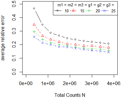
Then we move on to the setting where observations take discrete random values. High-dimensional count data commonly appear in a wide range of applications, including fluorescence microscopy, network flow, and microbiome (see, e.g., Nowak and Kolaczyk (2000); Jiang et al. (2015); Cao and Xie (2016); Cao et al. (2017), etc.), where Poisson and multinomial distributions are often used in modeling the counts. In this simulation study, we generate 𝐒∈ℝr1×r2×r3,Et∈ℝpt×rt{\mathbf{S}}\in\mathbb{R}^{r_{1}\times r_{2}\times r_{3}},E_{t}\in\mathbb{R}^{p_{t}\times r_{t}} as absolute values of i.i.d. standard normal random variables, and calculate

𝐗=𝐒×1E1×2E2×3E3∑i=1p1∑j=1p2∑k=1p3(𝐒×1E1×2E2×3E3)i​j​k.{\mathbf{X}}=\frac{{\mathbf{S}}\times_{1}E_{1}\times_{2}E_{2}\times_{3}E_{3}}{\sum_{i=1}^{p_{1}}\sum_{j=1}^{p_{2}}\sum_{k=1}^{p_{3}}\left({\mathbf{S}}\times_{1}E_{1}\times_{2}E_{2}\times_{3}E_{3}\right)_{ijk}}.

Ωt,Ξt\Omega_{t},\Xi_{t} are generated similarly as before, p1=p2=p3=50p_{1}=p_{2}=p_{3}=50, r1=r2=r3=3r_{1}=r_{2}=r_{3}=3, m1=m2=m3=g1=g2=g3∈{10,15,20,25}m_{1}=m_{2}=m_{3}=g_{1}=g_{2}=g_{3}\in\{10,15,20,25\}, and 𝐘=(𝐘i​j​k)1≤i≤p1,1≤j≤p2,1≤k≤p3{\mathbf{Y}}=({\mathbf{Y}}_{ijk})_{1\leq i\leq p_{1},1\leq j\leq p_{2},1\leq k\leq p_{3}} are Poisson or multinomial distributed:

𝐘i​j​k∼Poisson​(H​𝐗i​j​k),or𝐘i​j​k∼Multinomial​(N,𝐗).{\mathbf{Y}}_{ijk}\sim\text{Poisson}(H{\mathbf{X}}_{ijk}),\quad\text{or}\quad{\mathbf{Y}}_{ijk}\sim\text{Multinomial}(N;{\mathbf{X}}).

Here HH is a known intensity parameter in Poisson observations and NN is the total count parameter in multinomial observations. As shown in Figure 5, the proposed Algorithm 2 performs stably for these two types of noisy structures.

Although 𝐗{\mathbf{X}} is assumed to be exactly low-rank in all theoretical studies, it is not necessary in practice. In fact, our simulation study shows that Algorithm (2) performs well when 𝐗{\mathbf{X}} is only approximately low-rank. Specifically, we fix p1=p2=p3=50p_{1}=p_{2}=p_{3}=50, generate 𝐖∈ℝp1×p2×p3{\mathbf{W}}\in\mathbb{R}^{p_{1}\times p_{2}\times p_{3}} from i.i.d. standard normal, set U1∈𝕆p1,U2∈𝕆p2,U3∈𝕆p3U_{1}\in\mathbb{O}_{p_{1}},U_{2}\in\mathbb{O}_{p_{2}},U_{3}\in\mathbb{O}_{p_{3}} as uniform random orthogonal matrices, and Et=diag⁡(1,1,1−α,⋯,(pt−2)−α)E_{t}={\rm diag}(1,1,1^{-\alpha},\cdots,(p_{t}-2)^{-\alpha}). 𝐗{\mathbf{X}} is then constructed as

𝐗=𝐖×1(E1U1)×2(E2U2)×3(E3U3).{\mathbf{X}}={\mathbf{W}}\times_{1}\left(E_{1}U_{1}\right)\times_{2}\left(E_{2}U_{2}\right)\times_{3}\left(E_{3}U_{3}\right).

Here, α\alpha measures the decaying rate of singular values of each matricization of 𝐗{\mathbf{X}} and 𝐗{\mathbf{X}} becomes exactly rank-(3, 3, 3) when α=∞\alpha=\infty. We consider different decay rates α\alpha, noise levels σ\sigma, and observation set sizes mtm_{t} and gtg_{t}. The corresponding average relative Hilbert-Schmidt norm loss is reported in Figure 6. It can be seen that although 𝐗{\mathbf{X}} is not exactly low rank, as long as the singular values of each matricization of 𝐗{\mathbf{X}} decay sufficiently fast, a desirable completion of 𝐗{\mathbf{X}} can still be achieved, which again demonstrates the robustness of the proposed procedure.


Refer to caption
(a) Fixed mt=gt=10m_{t}=g_{t}=10, varying singular value decaying rate α\alpha and noise level σ\sigma.
Refer to caption
(b) Fixed σ=0.3\sigma=0.3, varying singular value decaying rate α\alpha and mt,gtm_{t},g_{t}.
Fig 6: Average relative loss for approximate low-rank tensors.

5 Real Data Illustration

In this section, we apply the proposed Cross tensor measurements scheme to a real dataset on attention hyperactivity disorder (ADHD) available from ADHD-200 Sample Initiative ( http://fcon_1000.projects.nitrc.org/indi/adhd200/). ADHD is a common disease that affects at least 5-7% of school-age children and may accompany patients throughout their life with direct costs of at least $36 billion per year in the United States. Despite being the most common mental disorder in children and adolescents, the cause of ADHD is largely unclear. To investigate the disease, the ADHD-200 study covered 285 subjects diagnosed with ADHD and 491 control subjects. After data cleaning, the dataset contains 776 tensors of dimension 121-by-145-by-121: 𝐘i,i=1,…,776{\mathbf{Y}}_{i},i=1,\dots,776. The storage space for these data through naive format is 121×145×121×776×4121\times 145\times 121\times 776\times 4B ≈\approx 6.137 GB, which makes it difficult and costly for sampling, storage and computation. Therefore, we hope to reduce the sampling size for ADHD brain imaging data via the proposed Cross tensor measurement scheme.

Figure 7 shows the singular values of each matricization of a randomly selected 𝐘i{\mathbf{Y}}_{i}. We can see that 𝐘i{\mathbf{Y}}_{i} is approximately Tucker low-rank.

Refer to caption
Refer to caption
Refer to caption
Fig 7: Singular value decompositions for each matricization of 𝐘{\mathbf{Y}}

Similar to previous simulation settings, we uniformly randomly select Ωt⊆[1:pt]\Omega_{t}\subseteq[1:p_{t}], Ξt⊆∏s≠tΩs\Xi_{t}\subseteq\prod_{s\neq t}\Omega_{s} such that |Ωt|=mt,|Ξt|=gt|\Omega_{t}|=m_{t},|\Xi_{t}|=g_{t}. Particularly, we choose mt=round​(ρ⋅pt),gt=round​(m1​m2​m3/pt)m_{t}=\text{round}(\rho\cdot p_{t}),\quad g_{t}=\text{round}(m_{1}m_{2}m_{3}/p_{t}), where ρ\rho varies from 0.1 to 0.5 and round(⋅\cdot) is the function that rounds its input to the nearest integer. After observing partial entries of each tensor, we apply Algorithm 2 with λt=3​pt/mt\lambda_{t}=3\sqrt{p_{t}/m_{t}} to obtain 𝐗^\hat{{\mathbf{X}}}. Different from some of the previous studies (e.g. Zhou et al. (2013)), our algorithm is adaptive and tuning-free so that we do not need to subjectively specify the rank of the target tensors beforehand.

Suppose rank⁡(𝐗^)=(r^1,r^2,r^3){\rm rank}(\hat{{\mathbf{X}}})=(\hat{r}_{1},\hat{r}_{2},\hat{r}_{3}), U^1∈𝕆p1,r1,U^2∈𝕆p2,r2,U^3∈𝕆p3,r3\hat{U}_{1}\in\mathbb{O}_{p_{1},r_{1}},\hat{U}_{2}\in\mathbb{O}_{p_{2},r_{2}},\hat{U}_{3}\in\mathbb{O}_{p_{3},r_{3}} are the left singular vectors of ℳ1​(𝐗^),ℳ2​(𝐗^),ℳ3​(𝐗^)\mathcal{M}_{1}(\hat{{\mathbf{X}}}),\mathcal{M}_{2}(\hat{{\mathbf{X}}}),\mathcal{M}_{3}(\hat{{\mathbf{X}}}), respectively. We are interested in investigating the performance of 𝐗^\hat{\mathbf{X}}, but the absence of the true tank of the underlying tensor 𝐗{\mathbf{X}} makes it difficult to directly compare 𝐗^\hat{{\mathbf{X}}} and 𝐗{\mathbf{X}}. Instead, we compare 𝐗^\hat{{\mathbf{X}}} with 𝐗~\tilde{{\mathbf{X}}}, where 𝐗~\tilde{{\mathbf{X}}} is the rank-(r^1,r^2,r^3)(\hat{r}_{1},\hat{r}_{2},\hat{r}_{3}) tensor obtained through the high-order singular value decomposition (HOSVD) (see e.g. Kolda and Bader (2009)) based on all observations in 𝐘{\mathbf{Y}}:

𝐗~=𝐘×1ℙU~1×2ℙU~2×3ℙU~3.\tilde{{\mathbf{X}}}={\mathbf{Y}}\times_{1}\mathbb{P}_{\tilde{U}_{1}}\times_{2}\mathbb{P}_{\tilde{U}_{2}}\times_{3}\mathbb{P}_{\tilde{U}_{3}}. (5.1)

Here U~1∈𝕆p1,r1,U~2∈𝕆p2,r2,U~3∈𝕆p3,r3\tilde{U}_{1}\in\mathbb{O}_{p_{1},r_{1}},\tilde{U}_{2}\in\mathbb{O}_{p_{2},r_{2}},\tilde{U}_{3}\in\mathbb{O}_{p_{3},r_{3}} are the first r1,r2r_{1},r_{2} and r3r_{3} left singular vectors of ℳ1​(𝐘)\mathcal{M}_{1}({\mathbf{Y}}), ℳ2​(𝐘)\mathcal{M}_{2}({\mathbf{Y}}) and ℳ3​(𝐘)\mathcal{M}_{3}({\mathbf{Y}}), respectively.

mtm_{t} Sampling Ratio(See (2.6))\begin{subarray}{c}\text{Sampling Ratio}\\ \text{(See \eqref{eq:sampling_ratio})}\end{subarray} ‖𝐗^−𝐘‖HS‖𝐗~−𝐘‖HS\frac{\|\hat{{\mathbf{X}}}-{\mathbf{Y}}\|_{\rm HS}}{\|\tilde{{\mathbf{X}}}-{\mathbf{Y}}\|_{\rm HS}} 1r^1​‖U^1⊤​U~1‖F\frac{1}{\sqrt{\hat{r}_{1}}}\|\hat{U}_{1}^{\top}\tilde{U}_{1}\|_{F} 1r^2​‖U^2⊤​U~2‖F\frac{1}{\sqrt{\hat{r}_{2}}}\|\hat{U}_{2}^{\top}\tilde{U}_{2}\|_{F} 1r^3​‖U^3⊤​U~3‖F\frac{1}{\sqrt{\hat{r}_{3}}}\|\hat{U}_{3}^{\top}\tilde{U}_{3}\|_{F}
round​(.1​pt)\text{round}(.1p_{t}) 0.0035 1.5086 0.8291 0.8212 0.8318
round​(.2​pt)\text{round}(.2p_{t}) 0.0267 1.2063 0.9352 0.9110 0.9155
round​(.3​pt)\text{round}(.3p_{t}) 0.0832 1.0918 0.9650 0.9571 0.9634
round​(.4​pt)\text{round}(.4p_{t}) 0.1766 1.0506 0.9769 0.9745 0.9828
round​(.5​pt)\text{round}(.5p_{t}) 0.3066 1.0312 0.9832 0.9840 0.9905
Table 1: Comparison between 𝐗^\hat{{\mathbf{X}}} and 𝐗~\tilde{{\mathbf{X}}} for ADHD brain imaging data.

Particularly, we compare ‖𝐗^−𝐘‖HS\|\hat{{\mathbf{X}}}-{\mathbf{Y}}\|_{\rm HS} and ‖𝐗~−𝐘‖HS\|\tilde{{\mathbf{X}}}-{\mathbf{Y}}\|_{\rm HS}, i.e. the rank-(r1,r2,r3)(r_{1},r_{2},r_{3}) approximation based on limited number of Cross tensor measurements and the approximation based on all measurements. We also compare U^1,U^2,U^3\hat{U}_{1},\hat{U}_{2},\hat{U}_{3} and U~1,U~2,U~3\tilde{U}_{1},\tilde{U}_{2},\tilde{U}_{3} by calculating 1r^t​‖U^t⊤​U~t‖F\frac{1}{\sqrt{\hat{r}_{t}}}\|\hat{U}_{t}^{\top}\tilde{U}_{t}\|_{F}. The study is performed on 10 randomly selected images and repeated 100 times for each of them. We can immediately see from the result in Table 1 that on average, ‖𝐗^−𝐘‖HS\|\hat{{\mathbf{X}}}-{\mathbf{Y}}\|_{\rm HS}, i.e. rank-(r1,r2,r3)(r_{1},r_{2},r_{3}) approximation error with limited numbers of Cross tensor measurements, can get very close to ‖𝐗~−𝐘‖HS\|\tilde{{\mathbf{X}}}-{\mathbf{Y}}\|_{\rm HS}, i.e. rank-(r1,r2,r3)(r_{1},r_{2},r_{3}) approximation error with the whole tensor 𝐘{\mathbf{Y}}. Besides, 1r^t​‖U^t⊤​U~t‖F\frac{1}{\sqrt{\hat{r}_{t}}}\|\hat{U}_{t}^{\top}\tilde{U}_{t}\|_{F} is close to 1, which means the singular vectors calculated from limited numbers of Cross tensor measurements are not too far from the ones calculated from the whole tensor.

Therefore, by the proposed Cross Tensor Measurement Scheme and a small fraction of observable entries, we can approximate the leading principle component of the original tensor just as if we have observed all voxels. This illustrates the power of the proposed algorithm.

6 Discussions: Extensions to Fourth and higher order Tensors

In this paper, we propose a novel tensor measurement scheme called Cross and the corresponding low-rank tensor completion algorithm. The theoretical analyses are provided for the proposed procedure to guarantee the optimality in both the sample size requirement and the completion error. The proposed procedure is efficient and easy to implement even for large-scale dataset.

Throughout the paper, we focus our presentations and analyses on order-3 tensors. Moreover, the proposed methods can be easily extended for fourth or higher order tensors. Suppose we aim to complete an unknown, order-dd, and rank-(r1,…,rd)(r_{1},\ldots,r_{d}) tensor: 𝐗∈ℝp1×⋯×pd{\mathbf{X}}\in\mathbb{R}^{p_{1}\times\cdots\times p_{d}}. Similarly, we introduce the order-dd Cross Tensor Measurement Scheme as

Ωt⊆[1:pt],where|Ωt|=mt,t=1,…,d,\Omega_{t}\subseteq[1:p_{t}],\quad\text{where}\quad|\Omega_{t}|=m_{t},\quad t=1,\ldots,d,
Ξt=∏s≠tΩs,where|Ξt|=gt,t=1,…,d,\Xi_{t}=\prod_{s\neq t}\Omega_{s},\quad\text{where}\quad|\Xi_{t}|=g_{t},\quad t=1,\ldots,d,
𝛀=(∏t=1dΩt)⋃t=1d([1:pt]×Ξt).\boldsymbol{\Omega}=\left(\prod_{t=1}^{d}\Omega_{t}\right)\bigcup\limits_{t=1}^{d}\left([1:p_{t}]\times\Xi_{t}\right).

By observing 𝐘𝛀=𝐗𝛀+𝐙𝛀{\mathbf{Y}}_{\boldsymbol{\Omega}}={\mathbf{X}}_{\boldsymbol{\Omega}}+{\mathbf{Z}}_{\boldsymbol{\Omega}}, we can construct the body, arm, and joint matricizations as

Yt,Ω=ℳt(𝐘[Ω1,…,Ωd]),YΞt=ℳt(𝐘[1:pt]×Ξt),YΩt×Ξt=ℳt(𝐘Ωt×Ξt).Y_{t,\Omega}=\mathcal{M}_{t}\left({\mathbf{Y}}_{[\Omega_{1},\ldots,\Omega_{d}]}\right),\quad Y_{\Xi_{t}}=\mathcal{M}_{t}\left({\mathbf{Y}}_{[1:p_{t}]\times\Xi_{t}}\right),\quad Y_{\Omega_{t}\times\Xi_{t}}=\mathcal{M}_{t}\left({\mathbf{Y}}_{\Omega_{t}\times\Xi_{t}}\right).

Similarly to Theorem 1, we can prove that 𝐗{\mathbf{X}} can be recovered by

𝐗^=𝐘[Ω1,…,Ωd]×1R1×2⋯×dRd,whereRt=YΞtYΩt×Ξt†,t=1,…,d,\hat{{\mathbf{X}}}={\mathbf{Y}}_{[\Omega_{1},\ldots,\Omega_{d}]}\times_{1}R_{1}\times_{2}\cdots\times_{d}R_{d},\quad\text{where}\quad R_{t}=Y_{\Xi_{t}}Y_{\Omega_{t}\times\Xi_{t}}^{\dagger},\quad t=1,\ldots,d,

in the noiseless setting, provided that min⁡{mt,gt}≥rt\min\{m_{t},g_{t}\}\geq r_{t} (so that |𝛀|≥∏t=1drt+∑t=1drt​(pt−rt)|\boldsymbol{\Omega}|\geq\prod_{t=1}^{d}r_{t}+\sum_{t=1}^{d}r_{t}(p_{t}-r_{t})) and some other mild assumptions holds. This result achieves the optimal sampling requirement since the degrees of freedom for rank-(r1,…,rd)(r_{1},\ldots,r_{d}) tensors in ℝp1×⋯×pd\mathbb{R}^{p_{1}\times\cdots\times p_{d}} is exactly ∏t=1drt+∑t=1drt​(pt−rt)\prod_{t=1}^{d}r_{t}+\sum_{t=1}^{d}r_{t}(p_{t}-r_{t}) (see Proposition 1 and Remark 1). Additionally, the procedure for order-dd tensor completion with noisy Cross measurements essentially follow from the proposed procedure in Algorithm 2, as long as we replace “t=1,2,3t=1,2,3” by “t=1,…,dt=1,\ldots,d”. An interesting problem for further exploration is on how to select the tuning parameter λt\lambda_{t} for the general order-dd tensor completion.

The main results on Cross tensor measurements can be further extended from the entry-wise observations to the more general projection settings. Suppose Pt∈𝕆pt,mtP_{t}\in\mathbb{O}_{p_{t},m_{t}} and Qt∈𝕆mt+1​mt+2,gtQ_{t}\in\mathbb{O}_{m_{t+1}m_{t+2},g_{t}} are orthogonal matrices for t=1,2,3t=1,2,3. We observe the following body, arm, and joint projections of 𝐗{\mathbf{X}},

𝐗(B)=𝐗×1P1⊤×2P2⊤×3P3⊤∈ℝm1×m2×m3,Xt(A)=ℳ1(𝐗×2P2⊤×3P3⊤)⋅Q1∈ℝpt×gt,t=1,2,3,Xt(J)=P1⊤⋅ℳ1(𝐗×2P2⊤×3P3⊤)⋅Q1∈ℝmt×gt,t=1,2,3.\begin{split}{\mathbf{X}}^{(B)}=&{\mathbf{X}}\times_{1}P_{1}^{\top}\times_{2}P_{2}^{\top}\times_{3}P_{3}^{\top}\in\mathbb{R}^{m_{1}\times m_{2}\times m_{3}},\\ X^{(A)}_{t}=&\mathcal{M}_{1}\left({\mathbf{X}}\times_{2}P_{2}^{\top}\times_{3}P_{3}^{\top}\right)\cdot Q_{1}\in\mathbb{R}^{p_{t}\times g_{t}},\quad t=1,2,3,\\ X^{(J)}_{t}=&P_{1}^{\top}\cdot\mathcal{M}_{1}\left({\mathbf{X}}\times_{2}P_{2}^{\top}\times_{3}P_{3}^{\top}\right)\cdot Q_{1}\in\mathbb{R}^{m_{t}\times g_{t}},\quad t=1,2,3.\end{split} (6.1)

The regular Cross tensor measurements discussed in Section 2.2 can be seen as a special case of (6.1), where

(Pt)i​j=1{i=Ωt(j)},1≤i≤pt,1≤j≤mt;(Qt)i​j=1{i=Ξt(j)},1≤i≤mt+1mt+2,1≤j≤gt.\begin{split}(P_{t})_{ij}=&1_{\{i=\Omega_{t}(j)\}},\quad 1\leq i\leq p_{t},\quad 1\leq j\leq m_{t};\\ (Q_{t})_{ij}=&1_{\{i=\Xi_{t}(j)\}},\quad 1\leq i\leq m_{t+1}m_{t+2},\quad 1\leq j\leq g_{t}.\end{split}

When 𝐗(B),Xt(A),Xt(J){\mathbf{X}}^{(B)},X_{t}^{(A)},X_{t}^{(J)} are observed without noise, by the similar argument of Theorem 1, one can show that

𝐗=𝐗(B)×1R1×R2×3R3,Rt=Xt(A)(Xt(J))†,t=1,2,3.{\mathbf{X}}={\mathbf{X}}^{(B)}\times_{1}R_{1}\times R_{2}\times_{3}R_{3},\quad R_{t}=X^{(A)}_{t}(X^{(J)}_{t})^{\dagger},\quad t=1,2,3.

In the noisy setting, one can similarly apply the proposed Algorithm 2 to recover 𝐗{\mathbf{X}}. Suppose the additive observation noises are

𝐙(B)=𝐘(B)−𝐗(B)∈ℝm1×m2×m3,Zt(A)=Yt(A)−Xt(A)∈ℝpt×gt,t=1,2,3,Zt(J)=Yt(J)−Xt(J)∈ℝmt×gt,t=1,2,3.\begin{split}{\mathbf{Z}}^{(B)}=&{\mathbf{Y}}^{(B)}-{\mathbf{X}}^{(B)}\in\mathbb{R}^{m_{1}\times m_{2}\times m_{3}},\\ Z_{t}^{(A)}=&Y_{t}^{(A)}-X_{t}^{(A)}\in\mathbb{R}^{p_{t}\times g_{t}},\quad t=1,2,3,\\ Z_{t}^{(J)}=&Y_{t}^{(J)}-X_{t}^{(J)}\in\mathbb{R}^{m_{t}\times g_{t}},\quad t=1,2,3.\end{split}

If 𝐗^\hat{{\mathbf{X}}} is the output from Algorithm 2, by similar procedure of Theorem 2, one can show that

‖𝐗^−𝐗‖HS≤C​λ1​λ2​λ3​‖𝐙(B)‖HS+C​λ1​λ2​λ3​(∑t=13ξt​‖Zt(J)‖F+C​∑t=13ξtλt​‖Zt(A)‖F).\begin{split}\left\|\hat{{\mathbf{X}}}-{\mathbf{X}}\right\|_{\rm HS}&\leq C\lambda_{1}\lambda_{2}\lambda_{3}\|{\mathbf{Z}}^{(B)}\|_{\rm HS}\\ &+C\lambda_{1}\lambda_{2}\lambda_{3}\left(\sum_{t=1}^{3}\xi_{t}\|Z_{t}^{(J)}\|_{F}+C\sum_{t=1}^{3}\frac{\xi_{t}}{\lambda_{t}}\|Z_{t}^{(A)}\|_{F}\right).\end{split} (6.2)

where λt≥2​‖X(A)​(Xt(J))†‖,ξt=‖(Xt(J))†​ℳt​(𝐗(B))‖\lambda_{t}\geq 2\|X^{(A)}(X^{(J)}_{t})^{\dagger}\|,\xi_{t}=\|(X^{(J)}_{t})^{\dagger}\mathcal{M}_{t}({\mathbf{X}}^{(B)})\|. This extension yields a possible application of Cross to general tensor estimation problems. Suppose one aims to recover low-rank tensor 𝐗{\mathbf{X}} from limited number of (not necessarily entry-wise) measurements. If one can obtain reasonable estimations for the following low-dimensional projections of 𝐗{\mathbf{X}},

𝐗(B)=𝐗×1P1×P2×P3∈ℝm1×m2×m3,andX(A)t=ℳt(𝐗×t+1Pt+1⊤×t+2Pt+2⊤)Qt∈ℝpt×gt,\begin{split}&{\mathbf{X}}^{(B)}={\mathbf{X}}\times_{1}P_{1}\times P_{2}\times P_{3}\in\mathbb{R}^{m_{1}\times m_{2}\times m_{3}},\\ ~~\text{and}~~&X^{(A)}_{t}=\mathcal{M}_{t}\left({\mathbf{X}}\times_{t+1}P_{t+1}^{\top}\times_{t+2}P_{t+2}^{\top}\right)Q_{t}\in\mathbb{R}^{p_{t}\times g_{t}},\end{split}

the proposed Algorithm 2 yields an efficient estimation for 𝐗{\mathbf{X}} with guaranteed performance (6.2). It would be an interesting future topic to apply Cross tensor measurement scheme to develop efficient algorithm for other low-rank tensor estimation problems, such as tensor completion with uniform random measurements, tensor regression and tensor denoising.

Acknowledgments

The author would like to thank Lexin Li for sharing the ADHD dataset and helpful discussion. The author would also like to thank the editor, associate editor, and anonymous referees for valuable suggestions on improving the paper.

References

  • Agarwal et al. (2012) Agarwal, A., Negahban, S., and Wainwright, M. J. (2012). Noisy matrix decomposition via convex relaxation: Optimal rates in high dimensions. The Annals of Statistics, pages 1171–1197.
  • Barak and Moitra (2016) Barak, B. and Moitra, A. (2016). Noisy tensor completion via the sum-of-squares hierarchy. In 29th Annual Conference on Learning Theory, pages 417–445.
  • Bhojanapalli and Sanghavi (2015) Bhojanapalli, S. and Sanghavi, S. (2015). A new sampling technique for tensors. arXiv preprint arXiv:1502.05023.
  • Cai et al. (2016) Cai, T., Cai, T. T., and Zhang, A. (2016). Structured matrix completion with applications to genomic data integration. Journal of the American Statistical Association, 111(514):621–633.
  • Cai and Zhang (2018) Cai, T. T. and Zhang, A. (2018). Rate-optimal perturbation bounds for singular subspaces with applications to high-dimensional statistics. The Annals of Statistics, 46(1):60–89.
  • Cai and Zhou (2016) Cai, T. T. and Zhou, W.-X. (2016). Matrix completion via max-norm constrained optimization. Electronic Journal of Statistics, 10(1):1493–1525.
  • Caiafa and Cichocki (2010) Caiafa, C. F. and Cichocki, A. (2010). Generalizing the column–row matrix decomposition to multi-way arrays. Linear Algebra and its Applications, 433(3):557–573.
  • Caiafa and Cichocki (2015) Caiafa, C. F. and Cichocki, A. (2015). Stable, robust, and super fast reconstruction of tensors using multi-way projections. IEEE Transactions on Signal Processing, 63(3):780–793.
  • Candes and Plan (2011) Candes, E. J. and Plan, Y. (2011). Tight oracle inequalities for low-rank matrix recovery from a minimal number of noisy random measurements. IEEE Transactions on Information Theory, 57(4):2342–2359.
  • Candès and Tao (2010) Candès, E. J. and Tao, T. (2010). The power of convex relaxation: Near-optimal matrix completion. IEEE Transactions on Information Theory, 56(5):2053–2080.
  • Cao and Xie (2016) Cao, Y. and Xie, Y. (2016). Poisson matrix recovery and completion. IEEE Transactions on Signal Processing, 64(6):1609–1620.
  • Cao et al. (2017) Cao, Y., Zhang, A., and Li, H. (2017). Microbial composition estimation from sparse count data. arXiv preprint arXiv:1706.02380.
  • Gandy et al. (2011) Gandy, S., Recht, B., and Yamada, I. (2011). Tensor completion and low-n-rank tensor recovery via convex optimization. Inverse Problems, 27(2):025010.
  • Gross and Nesme (2010) Gross, D. and Nesme, V. (2010). Note on sampling without replacing from a finite collection of matrices. arXiv preprint arXiv:1001.2738.
  • Guhaniyogi et al. (2017) Guhaniyogi, R., Qamar, S., and Dunson, D. B. (2017). Bayesian tensor regression. Journal of Machine Learning Research, (to appear).
  • Hillar and Lim (2013) Hillar, C. J. and Lim, L.-H. (2013). Most tensor problems are np-hard. Journal of the ACM (JACM), 60(6):45.
  • Jain and Oh (2014) Jain, P. and Oh, S. (2014). Provable tensor factorization with missing data. In Advances in Neural Information Processing Systems, pages 1431–1439.
  • Jiang et al. (2015) Jiang, X., Raskutti, G., and Willett, R. (2015). Minimax optimal rates for poisson inverse problems with physical constraints. IEEE Transactions on Information Theory, 61(8):4458–4474.
  • Johndrow et al. (2017) Johndrow, J. E., Bhattacharya, A., Dunson, D. B., et al. (2017). Tensor decompositions and sparse log-linear models. The Annals of Statistics, 45(1):1–38.
  • Karatzoglou et al. (2010) Karatzoglou, A., Amatriain, X., Baltrunas, L., and Oliver, N. (2010). Multiverse recommendation: n-dimensional tensor factorization for context-aware collaborative filtering. In Proceedings of the fourth ACM conference on Recommender systems, pages 79–86. ACM.
  • Keshavan et al. (2009) Keshavan, R. H., Oh, S., and Montanari, A. (2009). Matrix completion from a few entries. In 2009 IEEE International Symposium on Information Theory, pages 324–328. IEEE.
  • Klopp (2014) Klopp, O. (2014). Noisy low-rank matrix completion with general sampling distribution. Bernoulli, 20(1):282–303.
  • Kolda and Bader (2009) Kolda, T. G. and Bader, B. W. (2009). Tensor decompositions and applications. SIAM review, 51(3):455–500.
  • Koltchinskii et al. (2011) Koltchinskii, V., Lounici, K., and Tsybakov, A. B. (2011). Nuclear-norm penalization and optimal rates for noisy low-rank matrix completion. The Annals of Statistics, pages 2302–2329.
  • Kressner et al. (2014) Kressner, D., Steinlechner, M., and Vandereycken, B. (2014). Low-rank tensor completion by riemannian optimization. BIT Numerical Mathematics, 54(2):447–468.
  • Krishnamurthy and Singh (2013) Krishnamurthy, A. and Singh, A. (2013). Low-rank matrix and tensor completion via adaptive sampling. In Advances in Neural Information Processing Systems, pages 836–844.
  • Li et al. (2014) Li, L., Chen, Z., Wang, G., Chu, J., and Gao, H. (2014). A tensor prism algorithm for multi-energy ct reconstruction and comparative studies. Journal of X-ray science and technology, 22(2):147–163.
  • Li and Zhang (2016) Li, L. and Zhang, X. (2016). Parsimonious tensor response regression. Journal of the American Statistical Association, (just-accepted).
  • Li and Li (2010) Li, N. and Li, B. (2010). Tensor completion for on-board compression of hyperspectral images. In 2010 IEEE International Conference on Image Processing, pages 517–520. IEEE.
  • Li et al. (2013) Li, X., Zhou, H., and Li, L. (2013). Tucker tensor regression and neuroimaging analysis. arXiv preprint arXiv:1304.5637.
  • Liu et al. (2013) Liu, J., Musialski, P., Wonka, P., and Ye, J. (2013). Tensor completion for estimating missing values in visual data. IEEE Transactions on Pattern Analysis and Machine Intelligence, 35(1):208–220.
  • Mahoney et al. (2008) Mahoney, M. W., Maggioni, M., and Drineas, P. (2008). Tensor-cur decompositions for tensor-based data. SIAM Journal on Matrix Analysis and Applications, 30(3):957–987.
  • Mu et al. (2014) Mu, C., Huang, B., Wright, J., and Goldfarb, D. (2014). Square deal: Lower bounds and improved relaxations for tensor recovery. In ICML, pages 73–81.
  • Negahban and Wainwright (2011) Negahban, S. and Wainwright, M. J. (2011). Estimation of (near) low-rank matrices with noise and high-dimensional scaling. The Annals of Statistics, pages 1069–1097.
  • Negahban and Wainwright (2012) Negahban, S. and Wainwright, M. J. (2012). Restricted strong convexity and weighted matrix completion: Optimal bounds with noise. Journal of Machine Learning Research, 13(May):1665–1697.
  • Nowak and Kolaczyk (2000) Nowak, R. D. and Kolaczyk, E. D. (2000). A statistical multiscale framework for poisson inverse problems. IEEE Transactions on Information Theory, 46(5):1811–1825.
  • Oseledets et al. (2008) Oseledets, I. V., Savostianov, D., and Tyrtyshnikov, E. E. (2008). Tucker dimensionality reduction of three-dimensional arrays in linear time. SIAM Journal on Matrix Analysis and Applications, 30(3):939–956.
  • Oseledets and Tyrtyshnikov (2009) Oseledets, I. V. and Tyrtyshnikov, E. E. (2009). Breaking the curse of dimensionality, or how to use svd in many dimensions. SIAM Journal on Scientific Computing, 31(5):3744–3759.
  • Pimentel-Alarcón et al. (2016) Pimentel-Alarcón, D. L., Boston, N., and Nowak, R. D. (2016). A characterization of deterministic sampling patterns for low-rank matrix completion. IEEE Journal of Selected Topics in Signal Processing, 10(4):623–636.
  • Raskutti et al. (2017) Raskutti, G., Yuan, M., and Chen, H. (2017). Convex regularization for high-dimensional multi-response tensor regression. arXiv preprint arXiv:1512.01215v2.
  • Rauhut et al. (2016) Rauhut, H., Schneider, R., and Stojanac, Z. (2016). Low rank tensor recovery via iterative hard thresholding. arXiv preprint arXiv:1602.05217.
  • Recht (2011) Recht, B. (2011). A simpler approach to matrix completion. Journal of Machine Learning Research, 12(Dec):3413–3430.
  • Rendle and Schmidt-Thieme (2010) Rendle, S. and Schmidt-Thieme, L. (2010). Pairwise interaction tensor factorization for personalized tag recommendation. In Proceedings of the third ACM international conference on Web search and data mining, pages 81–90. ACM.
  • Richard and Montanari (2014) Richard, E. and Montanari, A. (2014). A statistical model for tensor pca. In Advances in Neural Information Processing Systems, pages 2897–2905.
  • Rohde et al. (2011) Rohde, A., Tsybakov, A. B., et al. (2011). Estimation of high-dimensional low-rank matrices. The Annals of Statistics, 39(2):887–930.
  • Rudelson and Vershynin (2007) Rudelson, M. and Vershynin, R. (2007). Sampling from large matrices: An approach through geometric functional analysis. Journal of the ACM (JACM), 54(4):21.
  • Semerci et al. (2014) Semerci, O., Hao, N., Kilmer, M. E., and Miller, E. L. (2014). Tensor-based formulation and nuclear norm regularization for multienergy computed tomography. IEEE Transactions on Image Processing, 23(4):1678–1693.
  • Shah et al. (2015) Shah, P., Rao, N., and Tang, G. (2015). Optimal low-rank tensor recovery from separable measurements: Four contractions suffice. arXiv preprint arXiv:1505.04085.
  • Srebro and Shraibman (2005) Srebro, N. and Shraibman, A. (2005). Rank, trace-norm and max-norm. In International Conference on Computational Learning Theory, pages 545–560. Springer.
  • Sun and Li (2016) Sun, W. W. and Li, L. (2016). Sparse low-rank tensor response regression. arXiv preprint arXiv:1609.04523.
  • Sun et al. (2015) Sun, W. W., Lu, J., Liu, H., and Cheng, G. (2015). Provable sparse tensor decomposition. Journal of Royal Statistical Association.
  • Tucker (1966) Tucker, L. R. (1966). Some mathematical notes on three-mode factor analysis. Psychometrika, 31(3):279–311.
  • Wagner and Zuk (2015) Wagner, A. and Zuk, O. (2015). Low-rank matrix recovery from row-and-column affine measurements. In Proceedings of the 32nd International Conference on Machine Learning (ICML-15), pages 2012–2020.
  • Wang and Singh (2015) Wang, Y. and Singh, A. (2015). Provably correct algorithms for matrix column subset selection with selectively sampled data. arXiv preprint arXiv:1505.04343.
  • Wetzstein et al. (2012) Wetzstein, G., Lanman, D., Hirsch, M., and Raskar, R. (2012). Tensor displays: compressive light field synthesis using multilayer displays with directional backlighting.
  • Weyl (1912) Weyl, H. (1912). Das asymptotische verteilungsgesetz der eigenwerte linearer partieller differentialgleichungen (mit einer anwendung auf die theorie der hohlraumstrahlung). Mathematische Annalen, 71(4):441–479.
  • Yuan and Zhang (2014) Yuan, M. and Zhang, C.-H. (2014). On tensor completion via nuclear norm minimization. Foundations of Computational Mathematics, pages 1–38.
  • Yuan and Zhang (2016) Yuan, M. and Zhang, C.-H. (2016). Incoherent tensor norms and their applications in higher order tensor completion. arXiv preprint arXiv:1606.03504.
  • Zhang et al. (2018) Zhang, A., Brown, L. D., and Cai, T. T. (2018). Semi-supervised inference: General theory and estimation of means. The Annals of Statistics, to appear.
  • Zhang and Xia (2018) Zhang, A. and Xia, D. (2018). Tensor svd: statistical and computational limits. IEEE Transactions on Information Theory, 64:1–28.
  • Zhou et al. (2013) Zhou, H., Li, L., and Zhu, H. (2013). Tensor regression with applications in neuroimaging data analysis. Journal of the American Statistical Association, 108(502):540–552.

Supplement to “Cross: Efficient Low-rank Tensor Completion”

Anru Zhang11 1 E-mail: anruzhang@stat.wisc.edu

University of Wisconsin-Madison

Abstract

  • In this Supplement, we provide proofs for the main results and technical lemmas. For better presentation for the long proof of Theorem 2, we also provide a table of used notations to Table 2.

A Proofs

We collect the proofs for the main results in this section.

A.1 Proof of Theorem 1

First, we shall note that 𝐘=𝐗{\mathbf{Y}}={\mathbf{X}} in the exact low-rank and noiseless setting. For each t=1,2,3t=1,2,3, according to definitions, XΞtX_{\Xi_{t}} is a collection of columns of ℳt​(𝐗)\mathcal{M}_{t}({\mathbf{X}}) and XΩt×ΞtX_{\Omega_{t}\times\Xi_{t}} is a collection of rows of XΞtX_{\Xi_{t}}. Then we have rank⁡(XΩt×Ξt)≤rank⁡(XΞt)≤rank⁡(ℳt​(𝐘)){\rm rank}(X_{\Omega_{t}\times\Xi_{t}})\leq{\rm rank}(X_{\Xi_{t}})\leq{\rm rank}(\mathcal{M}_{t}({\mathbf{Y}})). Given the assumptions, we have rank⁡(XΩt×Ξt)=rank⁡(ℳt​(𝐗))=rt{\rm rank}(X_{\Omega_{t}\times\Xi_{t}})={\rm rank}(\mathcal{M}_{t}({\mathbf{X}}))=r_{t}. Thus,

rank⁡(XΩt×Ξt)=rank⁡(XΞt)=rank⁡(ℳt​(𝐗))=rt.{\rm rank}(X_{\Omega_{t}\times\Xi_{t}})={\rm rank}(X_{\Xi_{t}})={\rm rank}(\mathcal{M}_{t}({\mathbf{X}}))=r_{t}.

Then ℳt​(𝐗)\mathcal{M}_{t}({\mathbf{X}}) and XΞtX_{\Xi_{t}} share the same column subspace and there exists a matrix Wt∈ℝgt×∏s≠tpsW_{t}\in\mathbb{R}^{g_{t}\times\prod_{s\neq t}p_{s}} such that ℳt​(𝐗)=XΞt⋅Wt.\mathcal{M}_{t}({\mathbf{X}})=X_{\Xi_{t}}\cdot W_{t}. On the other hand, since XΞtX_{\Xi_{t}} and XΩt×ΞtX_{\Omega_{t}\times\Xi_{t}} have the same row subspace, we have

XΞt=XΞt⋅(XΩt×Ξt)†⋅XΩt×Ξt=Rt⋅XΩt×Ξt.X_{\Xi_{t}}=X_{\Xi_{t}}\cdot(X_{\Omega_{t}\times\Xi_{t}})^{\dagger}\cdot X_{\Omega_{t}\times\Xi_{t}}=R_{t}\cdot X_{\Omega_{t}\times\Xi_{t}}. (A.1)

Additionally, XΞtX_{\Xi_{t}} and XΩt×ΞtX_{\Omega_{t}\times\Xi_{t}} can be factorized as XΞt=P1​QX_{\Xi_{t}}=P_{1}Q, XΩt×Ξt=P2​QX_{\Omega_{t}\times\Xi_{t}}=P_{2}Q, where P1∈ℝpt×rt,P2∈ℝmt×rtP_{1}\in\mathbb{R}^{p_{t}\times r_{t}},P_{2}\in\mathbb{R}^{m_{t}\times r_{t}}, Q∈ℝrt×gtQ\in\mathbb{R}^{r_{t}\times g_{t}} and rank⁡(P1)=rank⁡(P2)=rank⁡(Q)=rt{\rm rank}(P_{1})={\rm rank}(P_{2})={\rm rank}(Q)=r_{t}. In this case, for any matrices M~∈ℝmt×rt,N~∈ℝgt×rt\tilde{M}\in\mathbb{R}^{m_{t}\times r_{t}},\tilde{N}\in\mathbb{R}^{g_{t}\times r_{t}} with rank⁡(M~⊤​XΩt×Ξt​N~)=rt{\rm rank}(\tilde{M}^{\top}X_{\Omega_{t}\times\Xi_{t}}\tilde{N})=r_{t}, we have

R~t⋅XΩt×Ξt=XΞt​N~​(M~⊤​XΩt×Ξt​N~)−1​M~⊤⋅XΩt×Ξt=P1​Q​N~​(M~⊤​P2​Q​N~)−1​M~⊤​P2​Q=P1​Q​N~​(Q​N~)−1​(M~⊤​P2)−1​M~⊤​P2​Q=P1​Q=XΞt.\begin{split}\tilde{R}_{t}\cdot X_{\Omega_{t}\times\Xi_{t}}=&X_{\Xi_{t}}\tilde{N}\left(\tilde{M}^{\top}X_{\Omega_{t}\times\Xi_{t}}\tilde{N}\right)^{-1}\tilde{M}^{\top}\cdot X_{\Omega_{t}\times\Xi_{t}}\\ =&P_{1}Q\tilde{N}\left(\tilde{M}^{\top}P_{2}Q\tilde{N}\right)^{-1}\tilde{M}^{\top}P_{2}Q\\ =&P_{1}Q\tilde{N}(Q\tilde{N})^{-1}(\tilde{M}^{\top}P_{2})^{-1}\tilde{M}^{\top}P_{2}Q=P_{1}Q=X_{\Xi_{t}}.\end{split} (A.2)

Right multiplying WtW_{t} to (A.1) and (A.2), we obtain

ℳt​(𝐗)=XΞt⋅Wt=Rt⋅XΩt×Ξt⋅Wt=Rt⋅(ℳt(𝐘))[Ωt,:],=R~t⋅XΩt×Ξt⋅Wt=R~t⋅(ℳt(𝐘))[Ωt,:].\begin{split}\mathcal{M}_{t}({\mathbf{X}})=X_{\Xi_{t}}\cdot W_{t}=&R_{t}\cdot X_{\Omega_{t}\times\Xi_{t}}\cdot W_{t}=R_{t}\cdot\left(\mathcal{M}_{t}({\mathbf{Y}})\right)_{[\Omega_{t},:]},\\ =&\tilde{R}_{t}\cdot X_{\Omega_{t}\times\Xi_{t}}\cdot W_{t}=\tilde{R}_{t}\cdot\left(\mathcal{M}_{t}({\mathbf{Y}})\right)_{[\Omega_{t},:]}.\end{split}

By folding ℳt​(𝐗)\mathcal{M}_{t}({\mathbf{X}}) back to the tensors and Lemma 3, we obtain

𝐗=𝐗[Ω1,:,:]×1R1=𝐗[:,Ω2,:]×2R2=𝐗[:,:,Ω3]×3R3=𝐗[Ω1,:,:]×1R~1=𝐗[:,Ω2,:]×2R~2=𝐗[:,:,Ω3]×3R~3.\begin{split}{\mathbf{X}}=&{\mathbf{X}}_{[\Omega_{1},:,:]}\times_{1}R_{1}={\mathbf{X}}_{[:,\Omega_{2},:]}\times_{2}R_{2}={\mathbf{X}}_{[:,:,\Omega_{3}]}\times_{3}R_{3}\\ =&{\mathbf{X}}_{[\Omega_{1},:,:]}\times_{1}\tilde{R}_{1}={\mathbf{X}}_{[:,\Omega_{2},:]}\times_{2}\tilde{R}_{2}={\mathbf{X}}_{[:,:,\Omega_{3}]}\times_{3}\tilde{R}_{3}.\end{split}

By the equation above,

𝐗[Ω1,Ω2,Ω3]×1R1=𝐗[Ω1,Ω2,Ω3]×1R~1=𝐗[:,Ω2,Ω3],𝐗[:,Ω2,Ω3]×2R2=𝐗[:,Ω2,Ω3]×2R~2=𝐗[:,:,Ω3],𝐗[:,:,Ω3]×3R3=𝐗[:,:,Ω3]×3R~3=𝐗.\begin{split}&{\mathbf{X}}_{[\Omega_{1},\Omega_{2},\Omega_{3}]}\times_{1}R_{1}={\mathbf{X}}_{[\Omega_{1},\Omega_{2},\Omega_{3}]}\times_{1}\tilde{R}_{1}={\mathbf{X}}_{[:,\Omega_{2},\Omega_{3}]},\\ &{\mathbf{X}}_{[:,\Omega_{2},\Omega_{3}]}\times_{2}R_{2}={\mathbf{X}}_{[:,\Omega_{2},\Omega_{3}]}\times_{2}\tilde{R}_{2}={\mathbf{X}}_{[:,:,\Omega_{3}]},\\ &{\mathbf{X}}_{[:,:,\Omega_{3}]}\times_{3}R_{3}={\mathbf{X}}_{[:,:,\Omega_{3}]}\times_{3}\tilde{R}_{3}={\mathbf{X}}.\end{split}

Therefore,

𝐗[Ω1,Ω2,Ω3]×1R1×2R2×3R3=𝐗[Ω1,Ω2,Ω3]×1R~1×2R~2×3R~3=𝐗,{\mathbf{X}}_{[\Omega_{1},\Omega_{2},\Omega_{3}]}\times_{1}R_{1}\times_{2}R_{2}\times_{3}R_{3}={\mathbf{X}}_{[\Omega_{1},\Omega_{2},\Omega_{3}]}\times_{1}\tilde{R}_{1}\times_{2}\tilde{R}_{2}\times_{3}\tilde{R}_{3}={\mathbf{X}},

which concludes the proof of Theorem 1.  □\square

A.2 Proof of Theorem 2

Based on the proof for Theorem 1, we know

𝐗=𝐗[Ω1,Ω2,Ω3]×1R~1×2R~2×3R~3,{\mathbf{X}}={\mathbf{X}}_{[\Omega_{1},\Omega_{2},\Omega_{3}]}\times_{1}\tilde{R}_{1}\times_{2}\tilde{R}_{2}\times_{3}\tilde{R}_{3},

where

R~t=XΞt​N~​(M~⊤​XΩt×Ξt​N~)−1​M~⊤∈ℝpt×mt,\tilde{R}_{t}=X_{\Xi_{t}}\tilde{N}\left(\tilde{M}^{\top}X_{\Omega_{t}\times\Xi_{t}}\tilde{N}\right)^{-1}\tilde{M}^{\top}\in\mathbb{R}^{p_{t}\times m_{t}}, (A.3)

for any M~∈ℝmt×rt,N~∈ℝgt×rt\tilde{M}\in\mathbb{R}^{m_{t}\times r_{t}},\tilde{N}\in\mathbb{R}^{g_{t}\times r_{t}} satisfying M~⊤​XΩt×Ξt​N~\tilde{M}^{\top}X_{\Omega_{t}\times\Xi_{t}}\tilde{N} is non-singular. The proof for Theorem 2 is relatively long. For better presentation, we divide the proof into steps. Before going into detailed discussions, we list all notations with the definitions and possible simple explanations in Table 2 in the supplementary materials.

(Step 1.) Denote

N^t,Nt∈𝕆gt,rt​ as the first rt right singular vectors of YΞt, XΞt;M^t,Mt∈𝕆mt,rt​ as the first rt left singular vectors of Yt,Ω, Xt,Ω.\begin{split}\hat{N}_{t},N_{t}\in\mathbb{O}_{g_{t},r_{t}}\text{ as the first $r_{t}$ right singular vectors of $Y_{\Xi_{t}}$, $X_{\Xi_{t}}$};\\ \hat{M}_{t},M_{t}\in\mathbb{O}_{m_{t},r_{t}}\text{ as the first $r_{t}$ left singular vectors of $Y_{t,\Omega}$, $X_{t,\Omega}$}.\end{split} (A.4)

It is easy to see that alternate characterization for N^t\hat{N}_{t} and M^t\hat{M}_{t} are

N^t=V(A)[:,1:rt],M^t=U(B)[:,1:rt].\hat{N}_{t}=V^{(A)}_{[:,1:r_{t}]},\quad\hat{M}_{t}=U^{(B)}_{[:,1:r_{t}]}. (A.5)

Denote τ=1/5\tau=1/5. In this step, we prove that M^t,Mt\hat{M}_{t},M_{t}; N^t,Nt\hat{N}_{t},N_{t} are close by providing the upper bounds on singular subspace perturbations,

‖sin⁡Θ⁡(M^t,Mt)‖≤τ2/(1−2​τ),‖sin⁡Θ⁡(N^t,Nt)‖≤τ2/(1−2​τ);\|\sin\Theta(\hat{M}_{t},M_{t})\|\leq\tau^{2}/(1-2\tau),\quad\|\sin\Theta(\hat{N}_{t},N_{t})\|\leq\tau^{2}/(1-2\tau); (A.6)

as well as the inequality which ensures that JtJ_{t} is bounded away from being singular,

σmin​(M^t⊤​XΩt×Ξt​N^t)≥(1−τ4/(1−2​τ)2)​σmin​(XΩt×Ξt),σmin​(M^t⊤​YΩt×Ξt​N^t)≥(1−τ4/(1−2​τ)2−τ)​σmin​(XΩt×Ξt).\begin{split}\sigma_{\min}(\hat{M}_{t}^{\top}X_{\Omega_{t}\times\Xi_{t}}\hat{N}_{t})\geq&\left(1-\tau^{4}/(1-2\tau)^{2}\right)\sigma_{\min}(X_{\Omega_{t}\times\Xi_{t}}),\\ \sigma_{\min}(\hat{M}_{t}^{\top}Y_{\Omega_{t}\times\Xi_{t}}\hat{N}_{t})\geq&\left(1-\tau^{4}/(1-2\tau)^{2}-\tau\right)\sigma_{\min}(X_{\Omega_{t}\times\Xi_{t}}).\end{split} (A.7)

Actually, based on Assumption (3.1) , we have

σrt​(YΞt​Nt)≥σrt​(XΞt​Nt)−‖ZΞt​Nt‖≥σrt​(XΞt)−τ​σrt​(XΞt)=(1−τ)​σrt​(AΞt);\begin{split}&\sigma_{r_{t}}(Y_{\Xi_{t}}N_{t})\geq\sigma_{r_{t}}(X_{\Xi_{t}}N_{t})-\|Z_{\Xi_{t}}N_{t}\|\\ \geq&\sigma_{r_{t}}(X_{\Xi_{t}})-\tau\sigma_{r_{t}}(X_{\Xi_{t}})=(1-\tau)\sigma_{r_{t}}(A_{\Xi_{t}});\end{split}
σrt+1​(XΞt)≤σr+1​(XΞt)+‖ZΞt‖≤τ​σrt​(AΞt);\sigma_{r_{t}+1}(X_{\Xi_{t}})\leq\sigma_{r+1}(X_{\Xi_{t}})+\|Z_{\Xi_{t}}\|\leq\tau\sigma_{r_{t}}(A_{\Xi_{t}});
‖ℙXΞt​Nt​XΞt​(Nt)⟂‖≤‖XΞt​(Nt)⟂‖=‖AΞt​(Nt)⟂+ZΞt​(Nt)⟂‖≤‖ZΞt‖≤τ​σrt​(AΞt).\begin{split}&\left\|\mathbb{P}_{X_{\Xi_{t}}N_{t}}X_{\Xi_{t}}(N_{t})_{\perp}\right\|\leq\left\|X_{\Xi_{t}}(N_{t})_{\perp}\right\|=\left\|A_{\Xi_{t}}(N_{t})_{\perp}+Z_{\Xi_{t}}(N_{t})_{\perp}\right\|\\ \leq&\|Z_{\Xi_{t}}\|\leq\tau\sigma_{r_{t}}(A_{\Xi_{t}}).\end{split}

Here (Nt)⟂(N_{t})_{\perp} is the orthogonal complement matrix, i.e. [Nt​(Nt)⟂]∈𝕆gt[N_{t}~(N_{t})_{\perp}]\in\mathbb{O}_{g_{t}}. By setting A=XΞtA=X_{\Xi_{t}}, W=NtW=N_{t} in the scenario of the unilateral perturbation bound (Proposition 1 in Cai and Zhang (2018)), we then obtain

‖sin⁡Θ⁡(N^t,Nt)‖≤σrt+1​(XΞt)​‖ℙ(XΞt​Nt)​ZΞt​(Nt)⟂‖σrt2​(XΞt​Nt)−σrt+12​(XΞt)≤τ⋅τ(1−τ)2−τ2=τ2/(1−2​τ).\begin{split}&\left\|\sin\Theta(\hat{N}_{t},N_{t})\right\|\leq\frac{\sigma_{r_{t}+1}(X_{\Xi_{t}})\left\|\mathbb{P}_{(X_{\Xi_{t}}N_{t})}Z_{\Xi_{t}}(N_{t})_{\perp}\right\|}{\sigma_{r_{t}}^{2}(X_{\Xi_{t}}N_{t})-\sigma_{r_{t}+1}^{2}(X_{\Xi_{t}})}\\ \leq&\frac{\tau\cdot\tau}{(1-\tau)^{2}-\tau^{2}}=\tau^{2}/(1-2\tau).\end{split}

Here ‖sin⁡Θ⁡(⋅,⋅)‖\|\sin\Theta(\cdot,\cdot)\| is a commonly used distance between orthogonal subspaces. Similarly, based on the assumption that τ​σrt​(At,Ω)≥‖Zt,Ω‖\tau\sigma_{r_{t}}(A_{t,\Omega})\geq\|Z_{t,\Omega}\|, we can derive

‖sin⁡Θ⁡(M^t,Mt)‖≤τ2/(1−2​τ),\left\|\sin\Theta(\hat{M}_{t},M_{t})\right\|\leq\tau^{2}/(1-2\tau),

which proves (A.6). Based on the property for sin⁡Θ\sin\Theta distance (Lemma 1 in Cai and Zhang (2018)),

σmin​(N^t⊤​Nt)=1−‖sin⁡Θ⁡(N^t,Nt)‖2≥1−τ4​(1−2​τ)2;σmin​(M^t⊤​Mt)=1−‖sin⁡Θ⁡(M^t,Mt)‖2≥1−τ4/(1−2​τ)2.\begin{split}\sigma_{\min}(\hat{N}_{t}^{\top}N_{t})=\sqrt{1-\|\sin\Theta(\hat{N}_{t},N_{t})\|^{2}}\geq\sqrt{1-\tau^{4}(1-2\tau)^{2}};\\ \sigma_{\min}(\hat{M}_{t}^{\top}M_{t})=\sqrt{1-\|\sin\Theta(\hat{M}_{t},M_{t})\|^{2}}\geq\sqrt{1-\tau^{4}/(1-2\tau)^{2}}.\end{split}

Also, since Mt,NtM_{t},N_{t} coincide with the left and right singular subspaces of XΩt×ΞtX_{\Omega_{t}\times\Xi_{t}} respectively, we have

σmin​(M^t⊤​XΩt×Ξt​N^t)=σmin​(M^t⊤​ℙMt​XΩt×Ξt​ℙNt​N^t)=σmin​(M^t⊤​Mt​Mt⊤​XΩt×Ξt​Nt​Nt⊤​N^t)≥σmin​(M^t⊤​Mt)​σmin​(Mt⊤​XΩt×Ξt​Nt)​σmin​(Nt⊤​N^t)≥(1−τ4/(1−τ)2)​σmin​(XΩt×Ξt)\begin{split}&\sigma_{\min}(\hat{M}_{t}^{\top}X_{\Omega_{t}\times\Xi_{t}}\hat{N}_{t})\\ =&\sigma_{\min}(\hat{M}_{t}^{\top}\mathbb{P}_{M_{t}}X_{\Omega_{t}\times\Xi_{t}}\mathbb{P}_{N_{t}}\hat{N}_{t})=\sigma_{\min}(\hat{M}_{t}^{\top}M_{t}M_{t}^{\top}X_{\Omega_{t}\times\Xi_{t}}N_{t}N_{t}^{\top}\hat{N}_{t})\\ \geq&\sigma_{\min}(\hat{M}_{t}^{\top}M_{t})\sigma_{\min}(M_{t}^{\top}X_{\Omega_{t}\times\Xi_{t}}N_{t})\sigma_{\min}(N_{t}^{\top}\hat{N}_{t})\\ \geq&(1-\tau^{4}/(1-\tau)^{2})\sigma_{\min}(X_{\Omega_{t}\times\Xi_{t}})\end{split}
σmin​(M^t⊤​YΩt×Ξt​N^t)≥σmin​(M^t⊤​XΩt×Ξt​N^t)−‖ZΩt×Ξt‖≥(1−τ4/(1−2​τ)2−τ)​σmin​(XΩt×Ξt),\begin{split}&\sigma_{\min}(\hat{M}_{t}^{\top}Y_{\Omega_{t}\times\Xi_{t}}\hat{N}_{t})\geq\sigma_{\min}(\hat{M}_{t}^{\top}X_{\Omega_{t}\times\Xi_{t}}\hat{N}_{t})-\|Z_{\Omega_{t}\times\Xi_{t}}\|\\ \geq&(1-\tau^{4}/(1-2\tau)^{2}-\tau)\sigma_{\min}(X_{\Omega_{t}\times\Xi_{t}}),\end{split}

which has finished the proof for (A.7).

(Step 2.) In this step, we prove that under the given setting, r^t≥rt\hat{r}_{t}\geq r_{t} for t=1,2,3t=1,2,3. We only need to show that for each t=1,2,3t=1,2,3, the stopping criterion holds when s=rts=r_{t}, i.e.

‖(At)[:,1:rt](Jt)[1:rt,1:rt]−1‖≤λt.\left\|(A_{t})_{[:,1:r_{t}]}(J_{t})_{[1:r_{t},1:r_{t}]}^{-1}\right\|\leq\lambda_{t}. (A.8)

According to the definitions in (2.15), At,JtA_{t},J_{t} and M^t,N^t\hat{M}_{t},\hat{N}_{t} can be related as

(At)[:,1:rt]=YΞtV[:,1:rt](A)=(A.5)YΞtN^t=(XΞt+ZΞt)N^t,(A_{t})_{[:,1:r_{t}]}=Y_{\Xi_{t}}V^{(A)}_{[:,1:r_{t}]}\overset{\eqref{eq:hat_N_t_hat_M_t_U_V_related}}{=}Y_{\Xi_{t}}\hat{N}_{t}=(X_{\Xi_{t}}+Z_{\Xi_{t}})\hat{N}_{t},
(Jt)[1:rt,1:rt]=(U(B)[:,1:rt])⊤YΩt×ΞtV(A)[:,1:rt]=(A.5)M^t⊤YΩ×ΞtN^t=M^t⊤​(XΩ×Ξt+ZΩ×Ξt)​N^t.\begin{split}(J_{t})_{[1:r_{t},1:r_{t}]}=&(U^{(B)}_{[:,1:r_{t}]})^{\top}Y_{\Omega_{t}\times\Xi_{t}}V^{(A)}_{[:,1:r_{t}]}\overset{\eqref{eq:hat_N_t_hat_M_t_U_V_related}}{=}\hat{M}_{t}^{\top}Y_{\Omega\times\Xi_{t}}\hat{N}_{t}\\ =&\hat{M}_{t}^{\top}(X_{\Omega\times\Xi_{t}}+Z_{\Omega\times\Xi_{t}})\hat{N}_{t}.\end{split}

Therefore, in order to show (A.8), we only need to prove that M^t⊤​YΩt×Ξt​N^t\hat{M}_{t}^{\top}Y_{\Omega_{t}\times\Xi_{t}}\hat{N}_{t} is non-singular and

‖(XΞt+ZΞt)​N^t⋅(M^t⊤​(XΩt×Ξt+ZΩt×Ξt)​N^t)−1‖≤λt.\left\|(X_{\Xi_{t}}+Z_{\Xi_{t}})\hat{N}_{t}\cdot\left(\hat{M}_{t}^{\top}(X_{\Omega_{t}\times\Xi_{t}}+Z_{\Omega_{t}\times\Xi_{t}})\hat{N}_{t}\right)^{-1}\right\|\leq\lambda_{t}. (A.9)

Recall that Ut∈𝕆pt,rtU_{t}\in\mathbb{O}_{p_{t},r_{t}} is the singular subspace for ℳt​(𝐗)\mathcal{M}_{t}({\mathbf{X}}), so there exists another matrix Q∈ℝrt×gtQ\in\mathbb{R}^{r_{t}\times g_{t}} such that XΞtX_{\Xi_{t}}, a set of columns of ℳt​(𝐗)\mathcal{M}_{t}({\mathbf{X}}), can be written as

XΞt=Ut⋅Q, then XΩt×Ξt=Ut,Ω⋅Q.X_{\Xi_{t}}=U_{t}\cdot Q,\quad\text{ then }\quad X_{\Omega_{t}\times\Xi_{t}}=U_{t,\Omega}\cdot Q. (A.10)

Here Ut,Ω=(Ut)[Ωt,:]U_{t,\Omega}=(U_{t})_{[\Omega_{t},:]} is a collection of rows from UtU_{t}, and

XΞt​XΩt×Ξt†=Ut​Q​(Ut,Ω​Q)†=Ut​Ut,Ω†,then‖XΞt​XΩt×Ξt†‖=σmin−1​(Ut,Ω).X_{\Xi_{t}}X_{\Omega_{t}\times\Xi_{t}}^{\dagger}=U_{t}Q\left(U_{t,\Omega}Q\right)^{\dagger}=U_{t}U_{t,\Omega}^{\dagger},\quad\text{then}\quad\left\|X_{\Xi_{t}}X_{\Omega_{t}\times\Xi_{t}}^{\dagger}\right\|=\sigma_{\min}^{-1}(U_{t,\Omega}).

For convenience, we denote

λ¯t=1σmin​(Ut,Ω)=‖XΞt​XΩt×Ξt†‖​≤(3.3)​12​λt.\bar{\lambda}_{t}=\frac{1}{\sigma_{\min}(U_{t,\Omega})}=\left\|X_{\Xi_{t}}X_{\Omega_{t}\times\Xi_{t}}^{\dagger}\right\|\overset{\eqref{ineq:assumption_arm_body}}{\leq}\frac{1}{2}\lambda_{t}. (A.11)

In this case,

‖XΞt​N^t​(M^t⊤​XΩt×Ξt​N^t)−1‖=‖Ut​Q​N^t​(M^t⊤​Ut,Ω​Q​N^t)−1‖=‖Ut​(M^t⊤​Ut,Ω)−1‖=‖(M^t⊤​Ut,Ω)−1‖≤1σmin​(Ut,Ω)=λ¯t.\begin{split}&\left\|X_{\Xi_{t}}\hat{N}_{t}(\hat{M}_{t}^{\top}X_{\Omega_{t}\times\Xi_{t}}\hat{N}_{t})^{-1}\right\|=\left\|U_{t}Q\hat{N}_{t}(\hat{M}_{t}^{\top}U_{t,\Omega}Q\hat{N}_{t})^{-1}\right\|\\ =&\left\|U_{t}\left(\hat{M}_{t}^{\top}U_{t,\Omega}\right)^{-1}\right\|=\left\|\left(\hat{M}_{t}^{\top}U_{t,\Omega}\right)^{-1}\right\|\leq\frac{1}{\sigma_{\min}(U_{t,\Omega})}=\bar{\lambda}_{t}.\end{split} (A.12)

Furthermore,

σrt​(XΩ×Ξt)=σmin​(Ut,Ω⋅Q)≥σmin​(Ut,Ω)⋅σmin​(Q)=σmin​(Ut,Ω)⋅σmin​(Ut​Q)=σmin​(Ut,Ω)⋅σrt​(XΞt).\begin{split}&\sigma_{r_{t}}(X_{\Omega\times\Xi_{t}})=\sigma_{\min}(U_{t,\Omega}\cdot Q)\geq\sigma_{\min}(U_{t,\Omega})\cdot\sigma_{\min}(Q)\\ =&\sigma_{\min}(U_{t,\Omega})\cdot\sigma_{\min}(U_{t}Q)=\sigma_{\min}(U_{t,\Omega})\cdot\sigma_{r_{t}}(X_{\Xi_{t}}).\end{split} (A.13)

Therefore,

‖(XΞt+ZΞt)​N^t⋅(M^t⊤​(XΩt×Ξt+ZΩt×Ξt)​N^t)−1‖≤‖XΞt​N^t⋅(M^t⊤​(XΩt×Ξt+ZΩt×Ξt)​N^t)−1‖+‖ZΞt​N^t⋅(M^t⊤​(XΩt×Ξt+ZΩt×Ξt)​N^t)−1‖≤Lemma 5∥XΞtN^t⋅(M^t⊤XΩt×ΞtN^t)−1(M^t⊤ZΩt×ΞtN^t)⋅(M^⊤(XΩt×Ξt+ZΩt×Ξt)N^t)−1M^t∥+‖XΞt​N^t⋅(M^t⊤​XΩt×Ξt​N^t)−1‖+‖ZΞt‖σmin​(M^t⊤​YΩt×Ξt​N^t)≤(A.7)(A.12)λ¯t+λ¯t​‖ZΩt×Ξt‖(1−τ4/(1−2​τ)2−τ)​σmin​(XΩt×Ξt)+‖ZΞt‖(1−τ4/(1−2​τ)2−τ)​σmin​(XΩt×Ξt)≤(3.1)λ¯t+λ¯t​τ1−τ4/(1−2​τ)2−τ+τ​σrt​(XΞt)(1−τ4/(1−2​τ)2−τ)​σmin​(XΩt×Ξt)≤(A.13)λ¯t​(1+2​τ1−τ4/(1−2​τ)2−τ)​≤(A.11)​λt,\begin{split}&\left\|(X_{\Xi_{t}}+Z_{\Xi_{t}})\hat{N}_{t}\cdot\left(\hat{M}_{t}^{\top}\left(X_{\Omega_{t}\times\Xi_{t}}+Z_{\Omega_{t}\times\Xi_{t}}\right)\hat{N}_{t}\right)^{-1}\right\|\\ \leq&\left\|X_{\Xi_{t}}\hat{N}_{t}\cdot\left(\hat{M}_{t}^{\top}\left(X_{\Omega_{t}\times\Xi_{t}}+Z_{\Omega_{t}\times\Xi_{t}}\right)\hat{N}_{t}\right)^{-1}\right\|\\ &+\left\|Z_{\Xi_{t}}\hat{N}_{t}\cdot\left(\hat{M}_{t}^{\top}\left(X_{\Omega_{t}\times\Xi_{t}}+Z_{\Omega_{t}\times\Xi_{t}}\right)\hat{N}_{t}\right)^{-1}\right\|\\ \overset{\text{Lemma 5}}{\leq}&\Big\|X_{\Xi_{t}}\hat{N}_{t}\cdot\left(\hat{M}_{t}^{\top}X_{\Omega_{t}\times\Xi_{t}}\hat{N}_{t}\right)^{-1}\left(\hat{M}_{t}^{\top}Z_{\Omega_{t}\times\Xi_{t}}\hat{N}_{t}\right)\\ &\quad\quad\quad\cdot\left(\hat{M}^{\top}(X_{\Omega_{t}\times\Xi_{t}}+Z_{\Omega_{t}\times\Xi_{t}})\hat{N}_{t}\right)^{-1}\hat{M}_{t}\Big\|\\ &+\left\|X_{\Xi_{t}}\hat{N}_{t}\cdot\left(\hat{M}_{t}^{\top}X_{\Omega_{t}\times\Xi_{t}}\hat{N}_{t}\right)^{-1}\right\|+\frac{\|Z_{\Xi_{t}}\|}{\sigma_{\min}(\hat{M}_{t}^{\top}Y_{\Omega_{t}\times\Xi_{t}}\hat{N}_{t})}\\ \overset{\eqref{ineq:sigma_min-MXN}\eqref{ineq:X_leq_bar_lambda_t}}{\leq}&\bar{\lambda}_{t}+\bar{\lambda}_{t}\frac{\|Z_{\Omega_{t}\times\Xi_{t}}\|}{\left(1-\tau^{4}/(1-2\tau)^{2}-\tau\right)\sigma_{\min}(X_{\Omega_{t}\times\Xi_{t}})}\\ &+\frac{\|Z_{\Xi_{t}}\|}{\left(1-\tau^{4}/(1-2\tau)^{2}-\tau\right)\sigma_{\min}(X_{\Omega_{t}\times\Xi_{t}})}\\ \overset{\eqref{ineq:assumption_gap}}{\leq}&\bar{\lambda}_{t}+\frac{\bar{\lambda}_{t}\tau}{1-\tau^{4}/(1-2\tau)^{2}-\tau}\\ &+\frac{\tau\sigma_{r_{t}}(X_{\Xi_{t}})}{\left(1-\tau^{4}/(1-2\tau)^{2}-\tau\right)\sigma_{\min}(X_{\Omega_{t}\times\Xi_{t}})}\\ \overset{\eqref{ineq:sigma_rX_ratio}}{\leq}&\bar{\lambda}_{t}\left(1+\frac{2\tau}{1-\tau^{4}/(1-2\tau)^{2}-\tau}\right)\overset{\eqref{ineq:bar_lambda_t}}{\leq}\lambda_{t},\end{split}

which has proved our claim that r^t≥rt\hat{r}_{t}\geq r_{t} for t=1,2,3t=1,2,3.

(Step 3.) In this step, we provide an important decomposition of 𝐗^\hat{{\mathbf{X}}} under the scenario that r^t≥rt\hat{r}_{t}\geq r_{t}. One major difficulty is measuring the difference between Jt,[1:r^t,1:r^t]−1J_{t,[1:\hat{r}_{t},1:\hat{r}_{t}]}^{-1} and Jt,[1:rt,1:rt]−1J_{t,[1:r_{t},1:r_{t}]}^{-1}. For convenience, we further introduce the following notations,

Jr^t∈ℝr^t×r^t,Jr^t:=Jt,[1:r^t,1:r^t]=U(B)⊤t,[:,1:r^t]YΩt×ΞtVt,[:,1:r^t](A),J_{\hat{r}_{t}}\in\mathbb{R}^{\hat{r}_{t}\times\hat{r}_{t}},\quad J_{\hat{r}_{t}}:=J_{t,[1:\hat{r}_{t},1:\hat{r}_{t}]}=U^{(B)\top}_{t,[:,1:\hat{r}_{t}]}Y_{\Omega_{t}\times\Xi_{t}}V_{t,[:,1:\hat{r}_{t}]}^{(A)}, (A.14)
Jr^t(X):=U(B)⊤t,[:,1:r^t]XΩt×ΞtVt,[:,1:r^t],Jr^t(Z):=U(B)⊤t,[:,1:r^t]ZΩt×ΞtVt,[:,1:r^t],thenJr^t=Jr^t(X)+Jr^t(Z).\begin{split}J_{\hat{r}_{t}}^{(X)}:=&U^{(B)\top}_{t,[:,1:\hat{r}_{t}]}X_{\Omega_{t}\times\Xi_{t}}V_{t,[:,1:\hat{r}_{t}]},\quad J_{\hat{r}_{t}}^{(Z)}:=U^{(B)\top}_{t,[:,1:\hat{r}_{t}]}Z_{\Omega_{t}\times\Xi_{t}}V_{t,[:,1:\hat{r}_{t}]},\\ &\text{then}\quad J_{\hat{r}_{t}}=J_{\hat{r}_{t}}^{(X)}+J_{\hat{r}_{t}}^{(Z)}.\end{split} (A.15)
Ar^t∈ℝpt×r^t,Ar^t:=At,[:,1:r^t]=YΞtVt,[:,1:r^t](A),A_{\hat{r}_{t}}\in\mathbb{R}^{p_{t}\times\hat{r}_{t}},\quad A_{\hat{r}_{t}}:=A_{t,[:,1:\hat{r}_{t}]}=Y_{\Xi_{t}}V_{t,[:,1:\hat{r}_{t}]}^{(A)}, (A.16)
Ar^t(X):=XΞtV(A)t,[:,1:r^t],Ar^t(Z):=ZΞtV(A)t,[:,1:r^t],thenAr^t=Jr^t(X)+Jr^t(Z).A_{\hat{r}_{t}}^{(X)}:=X_{\Xi_{t}}V^{(A)}_{t,[:,1:\hat{r}_{t}]},\quad A_{\hat{r}_{t}}^{(Z)}:=Z_{\Xi_{t}}V^{(A)}_{t,[:,1:\hat{r}_{t}]},\quad\text{then}\quad A_{\hat{r}_{t}}=J_{\hat{r}_{t}}^{(X)}+J_{\hat{r}_{t}}^{(Z)}. (A.17)

Let the singular value decompositions of Jr^tJ_{\hat{r}_{t}} be

Jr^t=KtΛtLt⊤=[Kt​1Kt​2]⋅[Λt​1Λt​2]⋅[Lt​1⊤Lt​2⊤],t=1,2,3.J_{\hat{r}_{t}}=K_{t}\Lambda_{t}L_{t}^{\top}=\begin{bmatrix}K_{t1}&K_{t2}\end{bmatrix}\cdot\begin{bmatrix}\Lambda_{t1}&\\ &\Lambda_{t2}\end{bmatrix}\cdot\begin{bmatrix}L_{t1}^{\top}\\ L_{t2}^{\top}\end{bmatrix},\quad t=1,2,3. (A.18)

Here Kt,Lt∈𝕆r^tK_{t},L_{t}\in\mathbb{O}_{\hat{r}_{t}}, Kt​1,Lt​1∈𝕆r^t,rt,Kt​2,Lt​2∈𝕆r^t,rtK_{t1},L_{t1}\in\mathbb{O}_{\hat{r}_{t},r_{t}},K_{t2},L_{t2}\in\mathbb{O}_{\hat{r}_{t},r_{t}} are the singular vectors, Λt∈ℝr^t×r^t\Lambda_{t}\in\mathbb{R}^{\hat{r}_{t}\times\hat{r}_{t}}, Λt​1∈ℝrt×rt\Lambda_{t1}\in\mathbb{R}^{r_{t}\times r_{t}} and Λt​2∈ℝ(r^t−rt)×(r^t−rt)\Lambda_{t2}\in\mathbb{R}^{(\hat{r}_{t}-r_{t})\times(\hat{r}_{t}-r_{t})} are the singular values. Based on these SVDs, we can correspondingly decompose R¯t\bar{R}_{t} (defined in (2.17)) as

R¯t=At,[:,1:r^t]Jr^t−1U(B)t,[:,1:r^t]=At,[:,1:r^t](Kt​1Λt​1Lt​1⊤+Kt​2Λt​2Lt​2⊤)−1U(B)t,[:,1:r^t]=At,[:,1:r^t](Lt​1Λt​1−1Kt​1⊤+Lt​2Λt​2−1Kt​2⊤)U(B)t,[:,r^t]=At,[:,1:r^t]Lt​1Λt​1−1Kt​1⊤U(B)t,[:,1:r^t]+At,[:,1:r^t]Lt​2Λt​2−1Kt​2⊤U(B)t,[:,1:r^t]=YΞtVt,[:,1:r^t](A)Lt​1(Kt​1⊤Jr^tLt​1)−1Kt​1⊤U(B)t,[:,1:r^t]+YΞtVt,[:,1:r^t](A)Lt​2(Kt​2⊤Jr^tLt​2)−1Kt​2⊤U(B)t,[:,1:r^t].\begin{split}\bar{R}_{t}=&A_{t,[:,1:\hat{r}_{t}]}J_{\hat{r}_{t}}^{-1}U^{(B)}_{t,[:,1:\hat{r}_{t}]}=A_{t,[:,1:\hat{r}_{t}]}\left(K_{t1}\Lambda_{t1}L_{t1}^{\top}+K_{t2}\Lambda_{t2}L_{t2}^{\top}\right)^{-1}U^{(B)}_{t,[:,1:\hat{r}_{t}]}\\ =&A_{t,[:,1:\hat{r}_{t}]}\left(L_{t1}\Lambda_{t1}^{-1}K_{t1}^{\top}+L_{t2}\Lambda_{t2}^{-1}K_{t2}^{\top}\right)U^{(B)}_{t,[:,\hat{r}_{t}]}\\ =&A_{t,[:,1:\hat{r}_{t}]}L_{t1}\Lambda_{t1}^{-1}K_{t1}^{\top}U^{(B)}_{t,[:,1:\hat{r}_{t}]}+A_{t,[:,1:\hat{r}_{t}]}L_{t2}\Lambda_{t2}^{-1}K_{t2}^{\top}U^{(B)}_{t,[:,1:\hat{r}_{t}]}\\ =&Y_{\Xi_{t}}V_{t,[:,1:\hat{r}_{t}]}^{(A)}L_{t1}\left(K_{t1}^{\top}J_{\hat{r}_{t}}L_{t1}\right)^{-1}K_{t1}^{\top}U^{(B)}_{t,[:,1:\hat{r}_{t}]}\\ &+Y_{\Xi_{t}}V_{t,[:,1:\hat{r}_{t}]}^{(A)}L_{t2}\left(K_{t2}^{\top}J_{\hat{r}_{t}}L_{t2}\right)^{-1}K_{t2}^{\top}U^{(B)}_{t,[:,1:\hat{r}_{t}]}.\end{split} (A.19)

Here, the first term above associated with Kt​1,Lt​1​…K_{t1},L_{t1}... stands for the major part in R¯t\bar{R}_{t} while the second associated with Kt​2,Kt​2K_{t2},K_{t2} stands for the minor part. Based on this decomposition, we introduce the following notations: for any t=1,2,3t=1,2,3 (indicating Mode-1, 2 or 3) and s=1,2s=1,2 (indicating the major or minor parts),

At​s(X):=Ar^t(X)Lt​s=XΞtVt,[:,1:r^t](A)Lt​s,At​s(Z):=Ar^s(Z)Lt​s=ZΞtVt,[:,1:r^t](A)Lt​sA_{ts}^{(X)}:=A_{\hat{r}_{t}}^{(X)}L_{ts}=X_{\Xi_{t}}V_{t,[:,1:\hat{r}_{t}]}^{(A)}L_{ts},\quad A_{ts}^{(Z)}:=A_{\hat{r}_{s}}^{(Z)}L_{ts}=Z_{\Xi_{t}}V_{t,[:,1:\hat{r}_{t}]}^{(A)}L_{ts} (A.20)
At​s:=Ar^tLt​s=YΞtVt,[:,1:r^t](A)Lt​s=At​s(X)+At​s(Z).A_{ts}:=A_{\hat{r}_{t}}L_{ts}=Y_{\Xi_{t}}V_{t,[:,1:\hat{r}_{t}]}^{(A)}L_{ts}=A_{ts}^{(X)}+A_{ts}^{(Z)}. (A.21)
Jt​s(X):=Kt​s⊤Jr^tLt​s=Kt​s⊤Jr^t(X)Lt​s=Kt​s⊤U(B)⊤t,[:,1:r^t]XΩt×ΞtVt,[:,1:r^t](A)Lt​s,Jt​s(Z):=Kt​s⊤​Jr^t​Lt​s=Kt​s†​Ar^t​Lt​s=Kt​s⊤​Jr^t(A)​Lt​s=Kt​s⊤U(B)⊤t,[:,1:r^t]ZΩt×ΞtVt,[:,1:r^t](A)Lt​s,\begin{split}&J_{ts}^{(X)}:=K_{ts}^{\top}J_{\hat{r}_{t}}L_{ts}=K_{ts}^{\top}J_{\hat{r}_{t}}^{(X)}L_{ts}=K_{ts}^{\top}U^{(B)\top}_{t,[:,1:\hat{r}_{t}]}X_{\Omega_{t}\times\Xi_{t}}V_{t,[:,1:\hat{r}_{t}]}^{(A)}L_{ts},\\ &J_{ts}^{(Z)}:=K_{ts}^{\top}J_{\hat{r}_{t}}L_{ts}=K_{ts}^{\dagger}A_{\hat{r}_{t}}L_{ts}=K_{ts}^{\top}J_{\hat{r}_{t}}^{(A)}L_{ts}\\ &\quad\quad~=K_{ts}^{\top}U^{(B)\top}_{t,[:,1:\hat{r}_{t}]}Z_{\Omega_{t}\times\Xi_{t}}V_{t,[:,1:\hat{r}_{t}]}^{(A)}L_{ts},\end{split} (A.22)
Jt​s:=Jt​s(X)+Jt​s(Z)=Kt​s⊤U(B)⊤t,[:,1:r^t]YΩt×ΞtVt,[:,1:r^t](A)Lt​s.J_{ts}:=J_{ts}^{(X)}+J_{ts}^{(Z)}=K_{ts}^{\top}U^{(B)\top}_{t,[:,1:\hat{r}_{t}]}Y_{\Omega_{t}\times\Xi_{t}}V_{t,[:,1:\hat{r}_{t}]}^{(A)}L_{ts}. (A.23)

Also, for s1,s2,s3∈{1,2}3s_{1},s_{2},s_{3}\in\{1,2\}^{3}, we define the projected body measurements

𝐁s1​s2​s3(X)=𝐗[Ω1,Ω2,Ω3]×t=13(Kt​st⊤Ut,[1:r^t](B)){\mathbf{B}}^{(X)}_{s_{1}s_{2}s_{3}}={\mathbf{X}}_{[\Omega_{1},\Omega_{2},\Omega_{3}]}\times_{t=1}^{3}\left(K_{ts_{t}}^{\top}U_{t,[1:\hat{r}_{t}]}^{(B)}\right) (A.24)
𝐁s1​s2​s3(Z)=𝐙[Ω1,Ω2,Ω3]×t=13(Kt​st⊤Ut,[1:r^t](B)){\mathbf{B}}^{(Z)}_{s_{1}s_{2}s_{3}}={\mathbf{Z}}_{[\Omega_{1},\Omega_{2},\Omega_{3}]}\times_{t=1}^{3}\left(K_{ts_{t}}^{\top}U_{t,[1:\hat{r}_{t}]}^{(B)}\right) (A.25)
𝐁s1​s2​s3=𝐘[Ω1,Ω2,Ω3]×t=13(Kt​st⊤Ut,[1:r^t](B))=𝐁(X)s1​s2​s3+𝐁(Z)s1​s2​s3.\begin{split}{\mathbf{B}}_{s_{1}s_{2}s_{3}}=&{\mathbf{Y}}_{[\Omega_{1},\Omega_{2},\Omega_{3}]}\times_{t=1}^{3}\left(K_{ts_{t}}^{\top}U_{t,[1:\hat{r}_{t}]}^{(B)}\right)={\mathbf{B}}^{(X)}_{s_{1}s_{2}s_{3}}+{\mathbf{B}}^{(Z)}_{s_{1}s_{2}s_{3}}.\end{split} (A.26)

Combining (A.19)-(A.26), we can write down the following decomposition for 𝐗^\hat{{\mathbf{X}}}.

𝐗^=𝐘[Ω1,Ω2,Ω3]×1R¯1×2R¯2×3R¯3=(∑s1,s2,s3=12𝐁s1​s2​s3)×1(A11J11−1+A12J12−1)×2(A21J21−1+A22J22−1)×3(A31J31−1+A32J32−1)=∑s1,s2,s3=12𝐁s1​s2​s3×1A1​s1(J1​s1)−1×2A2​s2(J2​s2)−1×3A3​s3(J3​s3)−1.\begin{split}&\hat{{\mathbf{X}}}={\mathbf{Y}}_{[\Omega_{1},\Omega_{2},\Omega_{3}]}\times_{1}\bar{R}_{1}\times_{2}\bar{R}_{2}\times_{3}\bar{R}_{3}\\ =&\left(\sum_{s_{1},s_{2},s_{3}=1}^{2}{\mathbf{B}}_{s_{1}s_{2}s_{3}}\right)\times_{1}\left(A_{11}J_{11}^{-1}+A_{12}J_{12}^{-1}\right)\times_{2}\left(A_{21}J_{21}^{-1}+A_{22}J_{22}^{-1}\right)\\ &\quad\quad\quad\quad\quad\quad\quad\quad\quad\times_{3}\left(A_{31}J_{31}^{-1}+A_{32}J_{32}^{-1}\right)\\ =&\sum_{s_{1},s_{2},s_{3}=1}^{2}{\mathbf{B}}_{s_{1}s_{2}s_{3}}\times_{1}A_{1s_{1}}\left(J_{1s_{1}}\right)^{-1}\times_{2}A_{2s_{2}}\left(J_{2s_{2}}\right)^{-1}\times_{3}A_{3s_{3}}\left(J_{3s_{3}}\right)^{-1}.\end{split} (A.27)

This form is very helpful in our analysis later.

(Step 4.) In this step, we derive a few formulas for the terms in (A.27). To be specific, we shall prove the following results.

  • •

    Lower bound for singular value of the joint major part: for t=1,2,3t=1,2,3,

    σmin​(Jt​1(X))≥(1−τ12)​(1−τ4/(1−2​τ)2)​σmin​(XΩt×Ξt),τ1=τ2(1−τ4/(1−2​τ)2−τ)2−τ2.\begin{split}\sigma_{\min}\left(J_{t1}^{(X)}\right)\geq&(1-\tau_{1}^{2})(1-\tau^{4}/(1-2\tau)^{2})\sigma_{\min}(X_{\Omega_{t}\times\Xi_{t}}),\\ \tau_{1}=&\frac{\tau^{2}}{(1-\tau^{4}/(1-2\tau)^{2}-\tau)^{2}-\tau^{2}}.\end{split} (A.28)

    In fact, according to definitions, M^t⊤XΩt×ΞtN^t=(Jr^t(X))[1:rt,1:rt]\hat{M}_{t}^{\top}X_{\Omega_{t}\times\Xi_{t}}\hat{N}_{t}=(J_{\hat{r}_{t}}^{(X)})_{[1:r_{t},1:r_{t}]}, i.e., M^t⊤​XΩt×Ξt​N^t\hat{M}_{t}^{\top}X_{\Omega_{t}\times\Xi_{t}}\hat{N}_{t} is a sub-matrix of Jr^t(X)J_{\hat{r}_{t}}^{(X)}, we have

    σrt​(Jr^t(X))≥σrt​(M^⊤​XΩt×Ξt​N^)​=(A.7)​(1−τ4/(1−2​τ)2)​σmin​(XΩt×Ξt).\sigma_{r_{t}}(J_{\hat{r}_{t}}^{(X)})\geq\sigma_{r_{t}}\left(\hat{M}^{\top}X_{\Omega_{t}\times\Xi_{t}}\hat{N}\right)\overset{\eqref{ineq:sigma_min-MXN}}{=}(1-\tau^{4}/(1-2\tau)^{2})\sigma_{\min}(X_{\Omega_{t}\times\Xi_{t}}).

    Let

    K¯t∈𝕆r^t,rt,L¯t∈𝕆r^t,rt​ be the left and right singular vectorsfor rank-​rt​ matrix ​Jr^t(X).\begin{split}&\bar{K}_{t}\in\mathbb{O}_{\hat{r}_{t},r_{t}},\bar{L}_{t}\in\mathbb{O}_{\hat{r}_{t},r_{t}}\text{ be the left and right singular vectors}\\ &\text{for rank-}r_{t}\text{ matrix }J_{\hat{r}_{t}}^{(X)}.\end{split} (A.29)

    We summarize some facts here:

    • –

      Jr^t=Jr^t(X)+Jr^t(Z)J_{\hat{r}_{t}}=J_{\hat{r}_{t}}^{(X)}+J_{\hat{r}_{t}}^{(Z)};

    • –

      K¯t,L¯t\bar{K}_{t},\bar{L}_{t} are the left and right singular vectors of rank-rtr_{t} matrix Jr^t(X)J_{\hat{r}_{t}}^{(X)};

    • –

      Kt​1,Lt​1K_{t1},L_{t1} are the first rtr_{t} left and right singular vectors of Jr^tJ_{\hat{r}_{t}}.

    • –

      σrt+1​(Jr^t)​≤ Weyl (1912)​σrt+1​(Jr^t(X))+‖Jr^t(Z)‖≤τ​σmin​(XΩt×Ξt)\sigma_{r_{t}+1}(J_{\hat{r}_{t}})\overset{\text{ \cite[cite]{\@@bibref{Authors Phrase1YearPhrase2}{weyl1912asymptotische}{\@@citephrase{(}}{\@@citephrase{)}}}}}{\leq}\sigma_{r_{t}+1}(J_{\hat{r}_{t}}^{(X)})+\|J_{\hat{r}_{t}}^{(Z)}\|\leq\tau\sigma_{\min}(X_{\Omega_{t}\times\Xi_{t}}).

    • –

      σrt​(Jr^t​L¯t)​≥ Weyl (1912)​σrt​(Jr^t(X)​L¯t)−‖Jr^t(Z)‖=σrt​(Jr^t(X))−‖Jr^t(Z)‖\sigma_{r_{t}}(J_{\hat{r}_{t}}\bar{L}_{t})\overset{\text{ \cite[cite]{\@@bibref{Authors Phrase1YearPhrase2}{weyl1912asymptotische}{\@@citephrase{(}}{\@@citephrase{)}}}}}{\geq}\sigma_{r_{t}}(J_{\hat{r}_{t}}^{(X)}\bar{L}_{t})-\|J_{\hat{r}_{t}}^{(Z)}\|=\sigma_{r_{t}}(J_{\hat{r}_{t}}^{(X)})-\|J_{\hat{r}_{t}}^{(Z)}\|
      ≥(1−τ4/(1−2​τ)2−τ)​σmin​(XΩt×Ξt)\geq(1-\tau^{4}/(1-2\tau)^{2}-\tau)\sigma_{\min}(X_{\Omega_{t}\times\Xi_{t}}).

    Then by the unilateral perturbation bound result (Proposition 1 and Lemma 1 in Cai and Zhang (2018)) and the facts above,

    ‖sin⁡Θ⁡(L¯t,Lt​1)‖≤σrt+1​(Jr^t)⋅‖ℙ(Jr^t​L¯t)​Jr^t(Z)‖σrt2​(Jr^t​L¯t)−σrt+12​(Jr^t)≤(A.30)τ2(1−τ4/(1−2​τ)2−τ)2−τ2:=τ1.\begin{split}\left\|\sin\Theta(\bar{L}_{t},L_{t1})\right\|\leq&\frac{\sigma_{r_{t}+1}(J_{\hat{r}_{t}})\cdot\|\mathbb{P}_{(J_{\hat{r}_{t}}\bar{L}_{t})}J_{\hat{r}_{t}}^{(Z)}\|}{\sigma_{r_{t}}^{2}(J_{\hat{r}_{t}}\bar{L}_{t})-\sigma^{2}_{r_{t}+1}(J_{\hat{r}_{t}})}\\ \overset{\eqref{ineq:J_t1_Z}}{\leq}&\frac{\tau^{2}}{(1-\tau^{4}/(1-2\tau)^{2}-\tau)^{2}-\tau^{2}}:=\tau_{1}.\end{split}
    σmin​(Lt​1⊤​L¯t)≥1−τ12.\sigma_{\min}(L_{t1}^{\top}\bar{L}_{t})\geq\sqrt{1-\tau_{1}^{2}}.

    Similarly, σmin​(Kt​1⊤​K¯t)≥1−τ12\sigma_{\min}(K_{t1}^{\top}\bar{K}_{t})\geq\sqrt{1-\tau_{1}^{2}}. Therefore,

    σmin​(Jt​1(X))=σmin​(Kt​1⊤​Jr^t(X)​Lt​1)​=(A.29)​σmin​(Kt​1⊤​ℙK¯t​Jr^t(X)​ℙL¯t​Lt​1)=σmin​(Kt​1⊤​K¯t​K¯t⊤​Jr^t(X)​L¯t​L¯t⊤​Lt​1)≥σmin​(Kt​1⊤​K¯t)​σmin​(K¯t⊤​Jr^t(X)​L¯t)​σmin​(Lt​1⊤​L¯t)≥(1−τ12)​σrt​(Jr^t(X))≥(1−τ12)​(1−τ4/(1−2​τ)2)​σmin​(XΩt×Ξt).\begin{split}\sigma_{\min}\left(J_{t1}^{(X)}\right)=&\sigma_{\min}\left(K_{t1}^{\top}J_{\hat{r}_{t}}^{(X)}L_{t1}\right)\overset{\eqref{eq:def_K_t_L_t}}{=}\sigma_{\min}\left(K_{t1}^{\top}\mathbb{P}_{\bar{K}_{t}}J_{\hat{r}_{t}}^{(X)}\mathbb{P}_{\bar{L}_{t}}L_{t1}\right)\\ =&\sigma_{\min}\left(K_{t1}^{\top}\bar{K}_{t}\bar{K}_{t}^{\top}J_{\hat{r}_{t}}^{(X)}\bar{L}_{t}\bar{L}_{t}^{\top}L_{t1}\right)\\ \geq&\sigma_{\min}(K_{t1}^{\top}\bar{K}_{t})\sigma_{\min}\left(\bar{K}_{t}^{\top}J_{\hat{r}_{t}}^{(X)}\bar{L}_{t}\right)\sigma_{\min}(L_{t1}^{\top}\bar{L}_{t})\\ \geq&(1-\tau_{1}^{2})\sigma_{r_{t}}(J_{\hat{r}_{t}}^{(X)})\\ \geq&(1-\tau_{1}^{2})(1-\tau^{4}/(1-2\tau)^{2})\sigma_{\min}(X_{\Omega_{t}\times\Xi_{t}}).\end{split}

    which has finished the proof for (A.28).

  • •

    Upper bound for all terms related to perturbation “ZZ:” for example,

    ‖Jt​1(Z)‖≤‖ZΩt×Ξt‖≤τ​σmin​(XΩt×Ξt),\|J_{t1}^{(Z)}\|\leq\|Z_{\Omega_{t}\times\Xi_{t}}\|\leq\tau\sigma_{\min}(X_{\Omega_{t}\times\Xi_{t}}), (A.30)
    ‖At​1(Z)‖≤‖ZΞt‖≤τ​σmin​(XΞt).\|A_{t1}^{(Z)}\|\leq\|Z_{\Xi_{t}}\|\leq\tau\sigma_{\min}(X_{\Xi_{t}}).
    ‖𝐁s1​s2​s3(Z)‖HS≤‖𝐙[Ω1,Ω2,Ω3]‖HS,‖𝐁s1​s2​s3(Z)‖op≤‖𝐙[Ω1,Ω2,Ω3]‖op.\left\|{\mathbf{B}}_{s_{1}s_{2}s_{3}}^{(Z)}\right\|_{\rm HS}\leq\|{\mathbf{Z}}_{[\Omega_{1},\Omega_{2},\Omega_{3}]}\|_{\rm HS},\quad\left\|{\mathbf{B}}_{s_{1}s_{2}s_{3}}^{(Z)}\right\|_{\rm op}\leq\|{\mathbf{Z}}_{[\Omega_{1},\Omega_{2},\Omega_{3}]}\|_{\rm op}. (A.31)

    Since all these terms related to perturbation “(Z)(Z)” are essentially projections of ZΞtZ_{\Xi_{t}}, ZΩt×ΞtZ_{\Omega_{t}\times\Xi_{t}}, Zt,ΩZ_{t,\Omega} or 𝐙[Ω1,Ω2,Ω3]{\mathbf{Z}}_{[\Omega_{1},\Omega_{2},\Omega_{3}]}, they can be derived easily.

  • •

    Upper bounds in spectral norm for “arm ⋅\cdot joint-1” and “joint-1 ⋅\cdot body”:

    ‖At​1(X)​(Jt​1(X))−1‖≤λ¯t;\left\|A_{t1}^{(X)}(J_{t1}^{(X)})^{-1}\right\|\leq\bar{\lambda}_{t}; (A.32)
    if ​(s1,s2,s3)∈{1,2}3,t∈{1,2,3},‖(Jt​st(X))−1​ℳt​(𝐁s1​s2​s3(X))‖≤ξt;\text{if }(s_{1},s_{2},s_{3})\in\{1,2\}^{3},t\in\{1,2,3\},\quad\left\|(J^{(X)}_{ts_{t}})^{-1}\mathcal{M}_{t}({\mathbf{B}}_{s_{1}s_{2}s_{3}}^{(X)})\right\|\leq\xi_{t}; (A.33)
    ‖At​1​(Jt​1)−1‖≤λ¯t+2​λ¯t​τ(1−τ12)​(1−τ4/(1−2​τ)2)−τ;\left\|A_{t1}\left(J_{t1}\right)^{-1}\right\|\leq\bar{\lambda}_{t}+\frac{2\bar{\lambda}_{t}\tau}{(1-\tau_{1}^{2})(1-\tau^{4}/(1-2\tau)^{2})-\tau}; (A.34)
    ‖At​2​(Jt​2)−1‖≤λt+λ¯t+2​λ¯t​τ(1−τ12)​(1−τ4/(1−2​τ)2)−τ.\left\|A_{t2}\left(J_{t2}\right)^{-1}\right\|\leq\lambda_{t}+\bar{\lambda}_{t}+\frac{2\bar{\lambda}_{t}\tau}{(1-\tau_{1}^{2})(1-\tau^{4}/(1-2\tau)^{2})-\tau}. (A.35)

    Recall (A.10) that XΞt=Ut​QX_{\Xi_{t}}=U_{t}Q, XΩt×Ξt=Ut,Ω​QX_{\Omega_{t}\times\Xi_{t}}=U_{t,\Omega}Q, the definition for At​1(X)A_{t1}^{(X)}, Jt​1(X)J_{t1}^{(X)} and the fact that σmin​(Jt​1(X))>0\sigma_{\min}(J_{t1}^{(X)})>0, we have

    ‖At​1(X)​(Jt​1(X))−1‖=‖(XΞtV(A)t,[1:r^t]Lt​1)(Kt​1⊤Ut,[:,1:r^t](B)⊤XΩt×ΞtVt,[:,1:r^t](A)⊤Lt​1)−1‖=‖UtQV(A)t,[1:r^t]Lt​1(Kt​1⊤Ut,[:,1:r^t](B)⊤Ut,ΩQVt,[:,1:r^t](A)⊤Lt​1)−1‖=‖UtQV(A)t,[1:r^t]Lt​1(QVt,[:,1:r^t](A)⊤Lt​1)−1(Kt​1⊤Ut,[:,1:r^t](B)⊤Ut,Ω)−1‖=1σmin(Kt⊤U(B)⊤t,[:,1:r^t]Ut,Ω)≤1σmin​(Ut,Ω)=λ¯t,\begin{split}&\left\|A_{t1}^{(X)}(J_{t1}^{(X)})^{-1}\right\|\\ =&\left\|\left(X_{\Xi_{t}}V^{(A)}_{t,[1:\hat{r}_{t}]}L_{t1}\right)\left(K_{t1}^{\top}U_{t,[:,1:\hat{r}_{t}]}^{(B)\top}X_{\Omega_{t}\times\Xi_{t}}V_{t,[:,1:\hat{r}_{t}]}^{(A)\top}L_{t1}\right)^{-1}\right\|\\ =&\left\|U_{t}QV^{(A)}_{t,[1:\hat{r}_{t}]}L_{t1}\left(K_{t1}^{\top}U_{t,[:,1:\hat{r}_{t}]}^{(B)\top}U_{t,\Omega}QV_{t,[:,1:\hat{r}_{t}]}^{(A)\top}L_{t1}\right)^{-1}\right\|\\ =&\left\|U_{t}QV^{(A)}_{t,[1:\hat{r}_{t}]}L_{t1}\left(QV_{t,[:,1:\hat{r}_{t}]}^{(A)\top}L_{t1}\right)^{-1}\left(K_{t1}^{\top}U_{t,[:,1:\hat{r}_{t}]}^{(B)\top}U_{t,\Omega}\right)^{-1}\right\|\\ =&\frac{1}{\sigma_{\min}\left(K_{t}^{\top}U^{(B)\top}_{t,[:,1:\hat{r}_{t}]}U_{t,\Omega}\right)}\leq\frac{1}{\sigma_{\min}\left(U_{t,\Omega}\right)}=\bar{\lambda}_{t},\end{split}

    which has proved (A.32). The proof for (A.33) is similar. Since XΩt×ΞtX_{\Omega_{t}\times\Xi_{t}} is a collection of columns of Xt,ΩX_{t,\Omega} and rank⁡(XΩt×Ξt)=rank⁡(𝐗t,Ω)=rt{\rm rank}(X_{\Omega_{t}\times\Xi_{t}})={\rm rank}({\mathbf{X}}_{t,\Omega})=r_{t}, these two matrices share the same column subspace. In this case,

    XΩt×Ξt​(XΩt×Ξt†​Xt,Ω)=ℙXΩt×Ξt​Xt,Ω=Xt,Ω.X_{\Omega_{t}\times\Xi_{t}}\left(X_{\Omega_{t}\times\Xi_{t}}^{\dagger}X_{t,\Omega}\right)=\mathbb{P}_{X_{\Omega_{t}\times\Xi_{t}}}X_{t,\Omega}=X_{t,\Omega}.

    Given the assumption (3.3) that ‖XΩt×Ξt†​Xt,Ω‖≤ξt\|X_{\Omega_{t}\times\Xi_{t}}^{\dagger}X_{t,\Omega}\|\leq\xi_{t}, the rest of the proof for (A.33) essentially follows from the proof for (A.32).

    The proof for (A.34) is relatively more complicated. Note that

    ‖Jt​1(Z)‖≤‖ZΩt×Ξt‖≤τ​σmin​(XΩt×Ξt),‖At​1(Z)‖≤‖ZΞt‖≤τ​σrt​(XΞt)≤τ​σrt​(Q)=τ​σmin​(Q)≤τ​σmin​(Ut,Ω​Q)σmin​(Ut,Ω)≤τ​λ¯t​σmin​(XΩt×Ξt),\begin{split}\|J_{t1}^{(Z)}\|\leq&\|Z_{\Omega_{t}\times\Xi_{t}}\|\leq\tau\sigma_{\min}(X_{\Omega_{t}\times\Xi_{t}}),\\ \|A_{t1}^{(Z)}\|\leq&\|Z_{\Xi_{t}}\|\leq\tau\sigma_{r_{t}}(X_{\Xi_{t}})\leq\tau\sigma_{r_{t}}(Q)=\tau\sigma_{\min}(Q)\\ \leq&\frac{\tau\sigma_{\min}(U_{t,\Omega}Q)}{\sigma_{\min}(U_{t,\Omega})}\leq\tau\bar{\lambda}_{t}\sigma_{\min}(X_{\Omega_{t}\times\Xi_{t}}),\end{split} (A.36)

    we can calculate that

    ‖At​1​(Jt​1)−1‖=‖(At​1(X)+At​1(Z))​(Jt​1(X)+Jt​1(Z))−1‖≤‖At​1(X)​(Jt​1(X))−1‖+‖At​1(X)​((Jt​1(X)+Jt​1(Z))−1−(Jt​1(X))−1)‖+‖At​1(Z)​(Jt​1(X)+Jt​1(Z))−1‖=Lemma 5‖At​1(X)​(Jt​1(X))−1‖+‖At​1(X)​(Jt​1(X))−1​Jt​1(Z)​(Jt​1(X)+Jt​1(Z))−1‖+‖At​1(Z)‖​σmin−1​(Jt​1(X)+Jt​1(Z))=(A.32)λ¯t+λ¯t​‖Jt​1(Z)‖σmin​(Jt​1(X))−‖Jt​1(Z)‖+‖At​1(Z)‖σmin​(Jt​1(X))−‖Jt​1(Z)‖≤(A.36)(A.28)λ¯t+2​λ¯t​τ(1−τ12)​(1−τ4/(1−2​τ)2)−τ.\begin{split}&\left\|A_{t1}\left(J_{t1}\right)^{-1}\right\|=\left\|\left(A_{t1}^{(X)}+A_{t1}^{(Z)}\right)\left(J_{t1}^{(X)}+J_{t1}^{(Z)}\right)^{-1}\right\|\\ \leq&\left\|A_{t1}^{(X)}(J_{t1}^{(X)})^{-1}\right\|+\left\|A_{t1}^{(X)}\left(\left(J_{t1}^{(X)}+J_{t1}^{(Z)}\right)^{-1}-\left(J_{t1}^{(X)}\right)^{-1}\right)\right\|\\ &+\left\|A_{t1}^{(Z)}\left(J_{t1}^{(X)}+J_{t1}^{(Z)}\right)^{-1}\right\|\\ \overset{\text{Lemma 5}}{=}&\left\|A_{t1}^{(X)}(J_{t1}^{(X)})^{-1}\right\|+\left\|A_{t1}^{(X)}\left(J_{t1}^{(X)}\right)^{-1}J_{t1}^{(Z)}\left(J_{t1}^{(X)}+J_{t1}^{(Z)}\right)^{-1}\right\|\\ &+\left\|A_{t1}^{(Z)}\right\|\sigma_{\min}^{-1}\left(J_{t1}^{(X)}+J_{t1}^{(Z)}\right)\\ \overset{\eqref{ineq:A_t1^-1J_t1}}{=}&\bar{\lambda}_{t}+\bar{\lambda}_{t}\frac{\|J_{t1}^{(Z)}\|}{\sigma_{\min}(J_{t1}^{(X)})-\|J_{t1}^{(Z)}\|}+\frac{\|A_{t1}^{(Z)}\|}{\sigma_{\min}(J_{t1}^{(X)})-\|J_{t1}^{(Z)}\|}\\ \overset{\eqref{ineq:J_t1^Z, A_t1^Z leq}\eqref{ineq:sigma_min_J_t1}}{\leq}&\bar{\lambda}_{t}+\frac{2\bar{\lambda}_{t}\tau}{(1-\tau_{1}^{2})(1-\tau^{4}/(1-2\tau)^{2})-\tau}.\end{split}

    This has finished the proof for (A.34).

    Next, we move on to (A.35). Recall the definitions of Ar^tA_{\hat{r}_{t}} and Jr^tJ_{\hat{r}_{t}}, and the fact that Kt​1,Kt​2K_{t1},K_{t2}; Lt​1,Lt​2L_{t1},L_{t2} are orthogonal, we have Kt​1⊤​Kt​1=Lt​1⊤​Lt​1=IK_{t1}^{\top}K_{t1}=L_{t1}^{\top}L_{t1}=I, Kt​2⊤​Kt​2=Lt​2⊤​Lt​2=IK_{t2}^{\top}K_{t2}=L_{t2}^{\top}L_{t2}=I, Kt​1⊤​Kt​2=Lt​1⊤​Lt​2=0K_{t1}^{\top}K_{t2}=L_{t1}^{\top}L_{t2}=0. Then,

    Ar^t​Jr^t−1=(Ar^t​Lt​1​Lt​1⊤+Ar^t​Lt​2​Lt​2⊤)​(Kt​1​Kt​1⊤​Jr^t​Lt​1​Lt​1⊤+Kt​1​Kt​1⊤​Jr^t​Lt​2​Lt​2⊤)−1=(At​1​Lt​1⊤+At​2​Lt​2⊤)​(Kt​1​Jt​1​Lt​1⊤+Kt​2​Jt​2​Lt​2)−1=(At​1​Lt​1⊤+At​2​Lt​2⊤)​(Lt​1​Jt​1−1​Kt​1⊤+Lt​2​Jt​2−1​Kt​2)=At​1​Jt​1−1​Kt​1⊤+A21​Jt​2−1​Kt​2⊤.\begin{split}&A_{\hat{r}_{t}}J_{\hat{r}_{t}}^{-1}\\ =&\left(A_{\hat{r}_{t}}L_{t1}L_{t1}^{\top}+A_{\hat{r}_{t}}L_{t2}L_{t2}^{\top}\right)\left(K_{t1}K_{t1}^{\top}J_{\hat{r}_{t}}L_{t1}L_{t1}^{\top}+K_{t1}K_{t1}^{\top}J_{\hat{r}_{t}}L_{t2}L_{t2}^{\top}\right)^{-1}\\ =&\left(A_{t1}L_{t1}^{\top}+A_{t2}L_{t2}^{\top}\right)\left(K_{t1}J_{t1}L_{t1}^{\top}+K_{t2}J_{t2}L_{t2}\right)^{-1}\\ =&\left(A_{t1}L_{t1}^{\top}+A_{t2}L_{t2}^{\top}\right)\left(L_{t1}J_{t1}^{-1}K_{t1}^{\top}+L_{t2}J_{t2}^{-1}K_{t2}\right)\\ =&A_{t1}J_{t1}^{-1}K_{t1}^{\top}+A_{21}J_{t2}^{-1}K_{t2}^{\top}.\end{split}

    On the other hand, ‖Ar^t​Jr^t−1‖≤λt\left\|A_{\hat{r}_{t}}J_{\hat{r}_{t}}^{-1}\right\|\leq\lambda_{t}. Thus, (A.35) can shown by

    ‖At​2​(Jt​2)−1‖≤‖Ar^t​Jr^t−1‖+‖At​1​Jt​1−1​Kt​1⊤‖≤‖Ar^t​Jr^t−1‖+‖At​1​Jt​1−1‖≤λt+λ¯t+2​λ¯t​τ(1−τ12)​(1−τ4/(1−2​τ)2)−τ.\begin{split}&\left\|A_{t2}\left(J_{t2}\right)^{-1}\right\|\leq\left\|A_{\hat{r}_{t}}J_{\hat{r}_{t}}^{-1}\right\|+\left\|A_{t1}J_{t1}^{-1}K_{t1}^{\top}\right\|\\ \leq&\left\|A_{\hat{r}_{t}}J_{\hat{r}_{t}}^{-1}\right\|+\left\|A_{t1}J_{t1}^{-1}\right\|\leq\lambda_{t}+\bar{\lambda}_{t}+\frac{2\bar{\lambda}_{t}\tau}{(1-\tau_{1}^{2})(1-\tau^{4}/(1-2\tau)^{2})-\tau}.\end{split}
  • •

    Upper bounds in Frobenius and operator norm for “arm⋅\cdot(joint)-1⋅\cdotbody:” for the major part:

    ‖At​1​(Jt​1)−1​ℳt​(B111(X))−At​1(X)​(Jt​1(X))−1​ℳt​(B111(X))‖F≤C​λ¯t​ξt​‖ZΩt×Ξt‖F+C​ξt​‖ZΞt‖F.\begin{split}&\left\|A_{t1}\left(J_{t1}\right)^{-1}\mathcal{M}_{t}(B_{111}^{(X)})-A_{t1}^{(X)}\left(J_{t1}^{(X)}\right)^{-1}\mathcal{M}_{t}(B_{111}^{(X)})\right\|_{F}\\ \leq&C\bar{\lambda}_{t}\xi_{t}\|Z_{\Omega_{t}\times\Xi_{t}}\|_{F}+C\xi_{t}\|Z_{\Xi_{t}}\|_{F}.\end{split} (A.37)
    ‖At​1​(Jt​1)−1​ℳt​(B111(X))−At​1(X)​(Jt​1(X))−1​ℳt​(B111(X))‖≤C​λ¯t​ξt​‖ZΩt×Ξt‖+C​ξt​‖ZΞt‖.\begin{split}&\left\|A_{t1}\left(J_{t1}\right)^{-1}\mathcal{M}_{t}(B_{111}^{(X)})-A_{t1}^{(X)}\left(J_{t1}^{(X)}\right)^{-1}\mathcal{M}_{t}(B_{111}^{(X)})\right\|\\ \leq&C\bar{\lambda}_{t}\xi_{t}\|Z_{\Omega_{t}\times\Xi_{t}}\|+C\xi_{t}\|Z_{\Xi_{t}}\|.\end{split} (A.38)

    In order to show these two results, we need to use Lemma 5 and Zhang et al. (2018), which is an expansion formula for inverse matrix. Actually,

    ‖At​1​(Jt​1)−1​ℳt​(B111(X))−At​1(X)​(Jt​1(X))−1​ℳt​(B111(X))‖F=∥(At​1(X)+At​1(Z))(Jt​1(X)+Jt​1(Z))−1ℳt(B111(X))−At​1(X)(Jt​1(X))−1ℳt(B111(X))∥F≤‖At​1(X)​((Jt​1(X)+Jt​1(Z))−1−(Jt​1(X))−1)​ℳt​(B111(X))‖F+‖At​1(Z)​(Jt​1(X)+Jt​1(Z))−1​ℳt​(B111(X))‖F≤Lemma 5∥At​1(X)(Jt​1(X))−1(Jt​1(Z)−Jt​1(Z)(Jt​1(X)+Jt​1(Z))−1Jt​1(Z))⋅(Jt​1(X))−1ℳt(B111(X))∥F+‖At​1(Z)​(−(Jt​1(X)+Jt​1(Z))−1​Jt​1(Z)+I)​(Jt​1(X))−1​ℳt​(B111(X))‖F≤(A.32)(A.33)C​λ¯t​ξt​‖Jt​1(Z)−Jt​1(Z)​(Jt​1(X)+Jt​1(Z))−1​Jt​1(Z)‖F+Cξt‖At​1(Z)‖F⋅‖−(Jt​1(X)+Jt​1(Z))−1Jt​1(Z)+I‖≤(A.30)(A.28)C​λ¯t​ξt​‖Jt​1(Z)‖F+C​ξt​‖At​1(Z)‖F≤C​λ¯t​ξt​‖ZΩt×Ξt‖F+C​ξt​‖ZΞt‖F.\begin{split}&\left\|A_{t1}\left(J_{t1}\right)^{-1}\mathcal{M}_{t}(B_{111}^{(X)})-A_{t1}^{(X)}\left(J_{t1}^{(X)}\right)^{-1}\mathcal{M}_{t}(B_{111}^{(X)})\right\|_{F}\\ =&\Big\|(A_{t1}^{(X)}+A_{t1}^{(Z)})\left(J_{t1}^{(X)}+J_{t1}^{(Z)}\right)^{-1}\mathcal{M}_{t}(B_{111}^{(X)})\\ &\quad-A_{t1}^{(X)}\left(J_{t1}^{(X)}\right)^{-1}\mathcal{M}_{t}(B_{111}^{(X)})\Big\|_{F}\\ \leq&\left\|A_{t1}^{(X)}\left(\left(J_{t1}^{(X)}+J_{t1}^{(Z)}\right)^{-1}-\left(J_{t1}^{(X)}\right)^{-1}\right)\mathcal{M}_{t}(B_{111}^{(X)})\right\|_{F}\\ &+\left\|A_{t1}^{(Z)}\left(J_{t1}^{(X)}+J_{t1}^{(Z)}\right)^{-1}\mathcal{M}_{t}(B_{111}^{(X)})\right\|_{F}\\ \overset{\text{Lemma 5}}{\leq}&\Big\|A_{t1}^{(X)}\left(J_{t1}^{(X)}\right)^{-1}\left(J_{t1}^{(Z)}-J_{t1}^{(Z)}\left(J_{t1}^{(X)}+J_{t1}^{(Z)}\right)^{-1}J_{t1}^{(Z)}\right)\\ &\quad\quad\cdot\left(J_{t1}^{(X)}\right)^{-1}\mathcal{M}_{t}(B_{111}^{(X)})\Big\|_{F}\\ &+\left\|A_{t1}^{(Z)}\left(-\left(J_{t1}^{(X)}+J_{t1}^{(Z)}\right)^{-1}J_{t1}^{(Z)}+I\right)\left(J_{t1}^{(X)}\right)^{-1}\mathcal{M}_{t}(B_{111}^{(X)})\right\|_{F}\\ \overset{\eqref{ineq:A_t1^-1J_t1}\eqref{ineq:J_t1^-1B_111}}{\leq}&C\bar{\lambda}_{t}\xi_{t}\left\|J_{t1}^{(Z)}-J_{t1}^{(Z)}\left(J_{t1}^{(X)}+J_{t1}^{(Z)}\right)^{-1}J_{t1}^{(Z)}\right\|_{F}\\ &+C\xi_{t}\left\|A_{t1}^{(Z)}\right\|_{F}\cdot\left\|-\left(J_{t1}^{(X)}+J_{t1}^{(Z)}\right)^{-1}J_{t1}^{(Z)}+I\right\|\\ \overset{\eqref{ineq:J_t1_Z}\eqref{ineq:sigma_min_J_t1}}{\leq}&C\bar{\lambda}_{t}\xi_{t}\|J_{t1}^{(Z)}\|_{F}+C\xi_{t}\|A_{t1}^{(Z)}\|_{F}\leq C\bar{\lambda}_{t}\xi_{t}\|Z_{\Omega_{t}\times\Xi_{t}}\|_{F}+C\xi_{t}\|Z_{\Xi_{t}}\|_{F}.\end{split}

    which has proved (A.37). The proof for (A.38) essentially follows from the proof for (A.37) when we replace the Frobenius norms with the spectral norm.

  • •

    Upper bounds for minor “body” part:

    if ​(s1,s2,s3)∈{1,2}3​ and ​st=2,then {‖𝐁s1​s2​s3‖HS≤2​ξt​‖ZΩt×Ξt‖F+‖𝐙[Ω1,Ω2,Ω3]‖HS,‖𝐁s1​s2​s3‖op≤2​ξt​‖ZΩt×Ξt‖+‖𝐙[Ω1,Ω2,Ω3]‖op.\begin{split}&\text{if }(s_{1},s_{2},s_{3})\in\{1,2\}^{3}\text{ and }s_{t}=2,\quad\text{then }\\ &\left\{\begin{array}[]{ll}\left\|{\mathbf{B}}_{s_{1}s_{2}s_{3}}\right\|_{\rm HS}\leq 2\xi_{t}\left\|Z_{\Omega_{t}\times\Xi_{t}}\right\|_{F}+\left\|{\mathbf{Z}}_{[\Omega_{1},\Omega_{2},\Omega_{3}]}\right\|_{\rm HS},\\ \left\|{\mathbf{B}}_{s_{1}s_{2}s_{3}}\right\|_{\rm op}\leq 2\xi_{t}\left\|Z_{\Omega_{t}\times\Xi_{t}}\right\|+\left\|{\mathbf{Z}}_{[\Omega_{1},\Omega_{2},\Omega_{3}]}\right\|_{\rm op}.\end{array}\right.\end{split} (A.39)

    Instead of considering the “body” part above directly, we detour and discuss the “joint” part first. It is noteworthy that Jt​2J_{t2} is the rt+1,…,r^tr_{t}+1,\ldots,\hat{r}_{t}-th principle components for Jr^t=Jr^t(X)+Jr^t(Z)J_{\hat{r}_{t}}=J_{\hat{r}_{t}}^{(X)}+J_{\hat{r}_{t}}^{(Z)}. As rank⁡(Jr^t(X))=rt{\rm rank}(J_{\hat{r}_{t}}^{(X)})=r_{t}, by Lemma 1 in Cai et al. (2016) (which provides inequalities of singular values in the low-rank perturbed matrix),

    σi​(Jt​2)=σrt+i​(Jr^t)≤σi​(Jr^t(Z)),∀1≤i≤r^t−rt⇒‖Jt​2‖F=∑i=1r^t−rtσi2​(Jt​2)≤∑i=1r^t−rtσi2​(Jr^t(Z))=‖Jr^t(Z)‖F≤‖ZΩt×Ξt‖F,⇒‖Jt​2(X)‖F≤‖Jt​2‖F+‖Jt​2(Z)‖F≤2​‖ZΩt×Ξt‖F,⇒(A.33)‖ℳt​(𝐁s1​s2​s3(X))‖F≤‖Jt​2(X)‖F​‖(Jt​2(X))−1​ℳt​(𝐁s1​s2​s3(X))‖≤2​ξt​‖ZΩt×Ξt‖F⇒‖𝐁s1​s2​s3‖HS≤‖𝐁s1​s2​s3(X)‖HS+‖𝐁s1​s2​s3(Z)‖HS≤‖ℳt​(𝐁s1​s2​s3)‖F+‖𝐙[Ω1,Ω2,Ω3]‖HS≤2​ξt​‖ZΩt×Ξt‖F+‖𝐙[Ω1,Ω2,Ω3]‖HS.\begin{split}&\sigma_{i}(J_{t2})=\sigma_{r_{t}+i}(J_{\hat{r}_{t}})\leq\sigma_{i}(J_{\hat{r}_{t}}^{(Z)}),\quad\forall 1\leq i\leq\hat{r}_{t}-r_{t}\\ \Rightarrow\quad&\|J_{t2}\|_{F}=\sqrt{\sum_{i=1}^{\hat{r}_{t}-r_{t}}\sigma_{i}^{2}(J_{t2})}\leq\sqrt{\sum_{i=1}^{\hat{r}_{t}-r_{t}}\sigma_{i}^{2}(J_{\hat{r}_{t}}^{(Z)})}\\ &\quad\quad\quad=\|J_{\hat{r}_{t}}^{(Z)}\|_{F}\leq\|Z_{\Omega_{t}\times\Xi_{t}}\|_{F},\\ \Rightarrow\quad&\|J_{t2}^{(X)}\|_{F}\leq\|J_{t2}\|_{F}+\|J_{t2}^{(Z)}\|_{F}\leq 2\|Z_{\Omega_{t}\times\Xi_{t}}\|_{F},\\ \overset{\eqref{ineq:J_t1^-1B_111}}{\Rightarrow}\quad&\left\|\mathcal{M}_{t}({\mathbf{B}}^{(X)}_{s_{1}s_{2}s_{3}})\right\|_{F}\leq\left\|J_{t2}^{(X)}\right\|_{F}\left\|\left(J_{t2}^{(X)}\right)^{-1}\mathcal{M}_{t}({\mathbf{B}}^{(X)}_{s_{1}s_{2}s_{3}})\right\|\\ &\quad\quad\quad\quad\quad\quad\quad\leq 2\xi_{t}\|Z_{\Omega_{t}\times\Xi_{t}}\|_{F}\\ {\Rightarrow}\quad&\|{\mathbf{B}}_{s_{1}s_{2}s_{3}}\|_{\rm HS}\leq\left\|{\mathbf{B}}_{s_{1}s_{2}s_{3}}^{(X)}\right\|_{\rm HS}+\left\|{\mathbf{B}}_{s_{1}s_{2}s_{3}}^{(Z)}\right\|_{\rm HS}\\ &\quad\quad\quad\quad\quad\leq\|\mathcal{M}_{t}({\mathbf{B}}_{s_{1}s_{2}s_{3}})\|_{F}+\|{\mathbf{Z}}_{[\Omega_{1},\Omega_{2},\Omega_{3}]}\|_{\rm HS}\\ &\quad\quad\quad\quad\quad\leq 2\xi_{t}\|Z_{\Omega_{t}\times\Xi_{t}}\|_{F}+\|{\mathbf{Z}}_{[\Omega_{1},\Omega_{2},\Omega_{3}]}\|_{\rm HS}.\end{split}

    We can similarly derive that ‖𝐁s1​s2​s3‖op≤2​ξt​‖ZΩt×Ξt‖+‖𝐙[Ω1,Ω2,Ω3]‖op\|{\mathbf{B}}_{s_{1}s_{2}s_{3}}\|_{\rm op}\leq 2\xi_{t}\|Z_{\Omega_{t}\times\Xi_{t}}\|+\|{\mathbf{Z}}_{[\Omega_{1},\Omega_{2},\Omega_{3}]}\|_{\rm op}, which has proved (A.39).

  • •

    Equality for the original tensor 𝐗{\mathbf{X}}:

    𝐗=𝐁111(X)×1A11(X)(J11(X))−1×2A21(X)(J21(X))−1×3A31(X)(J31(X))−1.{\mathbf{X}}={\mathbf{B}}_{111}^{(X)}\times_{1}A_{11}^{(X)}\left(J_{11}^{(X)}\right)^{-1}\times_{2}A_{21}^{(X)}\left(J_{21}^{(X)}\right)^{-1}\times_{3}A_{31}^{(X)}\left(J_{31}^{(X)}\right)^{-1}. (A.40)

    In fact, according to the definitions (A.20) - (A.26),

    𝐁111(X)×1A11(X)×2A21(X)×3A31(X)=𝐗[Ω1,Ω2,Ω3]×t=13{XΞt(Vt,[:,1:r^t](A)Lt​1)⋅((U(B)t,[:,1:r^t]Kt​1)⊤XΩt×Ξt(Vt,[:,1:r^t](A)Lt​1))−1(U(B)1,[:,1:r^1]K11)⊤}\begin{split}&{\mathbf{B}}_{111}^{(X)}\times_{1}A_{11}^{(X)}\times_{2}A_{21}^{(X)}\times_{3}A_{31}^{(X)}\\ =&{\mathbf{X}}_{[\Omega_{1},\Omega_{2},\Omega_{3}]}\times_{t=1}^{3}\Bigg\{X_{\Xi_{t}}\left(V_{t,[:,1:\hat{r}_{t}]}^{(A)}L_{t1}\right)\\ &\quad\quad\quad\cdot\left(\left(U^{(B)}_{t,[:,1:\hat{r}_{t}]}K_{t1}\right)^{\top}X_{\Omega_{t}\times\Xi_{t}}\left(V_{t,[:,1:\hat{r}_{t}]}^{(A)}L_{t1}\right)\right)^{-1}\left(U^{(B)}_{1,[:,1:\hat{r}_{1}]}K_{11}\right)^{\top}\Bigg\}\\ \end{split}

    Based on (A.28), Jt​1(X)=Kt​1⊤(U1,[:,1:r^t](B))⊤XΩt×ΞtVt,[:,1:r^t](A)Lt​1J_{t1}^{(X)}=K_{t1}^{\top}(U^{(B)}_{1,[:,1:\hat{r}_{t}]})^{\top}X_{\Omega_{t}\times\Xi_{t}}V_{t,[:,1:\hat{r}_{t}]}^{(A)}L_{t1} is non-singular, then by Theorem 1, we can show the term above equals 𝐗{\mathbf{X}}, which has proved (A.40).

(Step 5.) Now we are ready to analyze the estimation error of 𝐗^\hat{{\mathbf{X}}} based on all the preparations in the previous steps. Based on the decompositions of 𝐗^\hat{{\mathbf{X}}} (A.27) and 𝐗{\mathbf{X}} (A.40), one has

‖𝐗^−𝐗‖HS≤∥𝐁111×1A11J11−1×2A21J21−1×3A31J31−1−𝐁111(X)×1A11(X)(J11(X))−1×2A21(X)(J21(X))−1×3A31(X)(J31(X))−1∥HS+∑s1,s2,s3=1(s1,s2,s3)≠(1,1,1)2‖𝐁s1​s2​s3×1A1​s1J1​s1−1×2A2​s2J2​s2−1×3A3​s3J3​s3−1‖HS≤‖(𝐁111−𝐁111(X))×1A11J11−1×2A21J21−1×3A31J31−1‖HS+‖𝐁111(X)×1A11J11−1×2A21J21−1×3(A31J31−1−A31(X)(J31(X))−1)‖HS+‖𝐁111(X)×1A11J11−1×2(A21J21−1−A21(X)J21(X)−1)×3A31(X)J31(X)−1‖HS+‖𝐁111(X)×1(A11J11−1−A11(X)J11(X)−1)×2A21(X)J21(X)−1×3A31(X)J31(X)−1‖HS+∑s1,s2,s3=1(s1,s2,s3)≠(1,1,1)2‖𝐁s1​s2​s3×1A1​s1J1​s1−1×2A2​s2J2​s2−1×3A3​s3J3​s3−1‖HS.\begin{split}&\left\|\hat{{\mathbf{X}}}-{\mathbf{X}}\right\|_{\rm HS}\\ \leq&\Big\|{\mathbf{B}}_{111}\times_{1}A_{11}J_{11}^{-1}\times_{2}A_{21}J_{21}^{-1}\times_{3}A_{31}J_{31}^{-1}\\ &-{\mathbf{B}}_{111}^{(X)}\times_{1}A_{11}^{(X)}\left(J_{11}^{(X)}\right)^{-1}\times_{2}A_{21}^{(X)}\left(J_{21}^{(X)}\right)^{-1}\times_{3}A_{31}^{(X)}\left(J_{31}^{(X)}\right)^{-1}\Big\|_{\rm HS}\\ &+\sum_{\begin{subarray}{c}s_{1},s_{2},s_{3}=1\\ (s_{1},s_{2},s_{3})\neq(1,1,1)\end{subarray}}^{2}\left\|{\mathbf{B}}_{s_{1}s_{2}s_{3}}\times_{1}A_{1s_{1}}J_{1s_{1}}^{-1}\times_{2}A_{2s_{2}}J_{2s_{2}}^{-1}\times_{3}A_{3s_{3}}J_{3s_{3}}^{-1}\right\|_{\rm HS}\\ \leq&\left\|\left({\mathbf{B}}_{111}-{\mathbf{B}}_{111}^{(X)}\right)\times_{1}A_{11}J_{11}^{-1}\times_{2}A_{21}J_{21}^{-1}\times_{3}A_{31}J_{31}^{-1}\right\|_{\rm HS}\\ &+\left\|{\mathbf{B}}_{111}^{(X)}\times_{1}A_{11}J_{11}^{-1}\times_{2}A_{21}J_{21}^{-1}\times_{3}\left(A_{31}J_{31}^{-1}-A_{31}^{(X)}(J_{31}^{(X)})^{-1}\right)\right\|_{\rm HS}\\ &+\left\|{\mathbf{B}}_{111}^{(X)}\times_{1}A_{11}J_{11}^{-1}\times_{2}\left(A_{21}J_{21}^{-1}-A_{21}^{(X)}J_{21}^{(X)-1}\right)\times_{3}A_{31}^{(X)}J_{31}^{(X)-1}\right\|_{\rm HS}\\ &+\left\|{\mathbf{B}}_{111}^{(X)}\times_{1}\left(A_{11}J_{11}^{-1}-A_{11}^{(X)}J_{11}^{(X)-1}\right)\times_{2}A_{21}^{(X)}J_{21}^{(X)-1}\times_{3}A_{31}^{(X)}J_{31}^{(X)-1}\right\|_{\rm HS}\\ &+\sum_{\begin{subarray}{c}s_{1},s_{2},s_{3}=1\\ (s_{1},s_{2},s_{3})\neq(1,1,1)\end{subarray}}^{2}\left\|{\mathbf{B}}_{s_{1}s_{2}s_{3}}\times_{1}A_{1s_{1}}J_{1s_{1}}^{-1}\times_{2}A_{2s_{2}}J_{2s_{2}}^{-1}\times_{3}A_{3s_{3}}J_{3s_{3}}^{-1}\right\|_{\rm HS}.\end{split} (A.41)

For each term separately above, we have

‖(𝐁111−𝐁111(X))×1A11J11−1×2A21J21−1×3A31J31−1‖HS≤‖A11​J11−1‖⋅‖A21​J21−1‖⋅‖A31​J31−1‖​‖𝐁111(Z)‖HS≤(A.31)(A.32)​C​λ1​λ2​λ3​‖𝐙[Ω1,Ω2,Ω3]‖HS.\begin{split}&\quad\quad\ \left\|\left({\mathbf{B}}_{111}-{\mathbf{B}}_{111}^{(X)}\right)\times_{1}A_{11}J_{11}^{-1}\times_{2}A_{21}J_{21}^{-1}\times_{3}A_{31}J_{31}^{-1}\right\|_{\rm HS}\\ &~~\quad\leq\left\|A_{11}J_{11}^{-1}\right\|\cdot\left\|A_{21}J_{21}^{-1}\right\|\cdot\left\|A_{31}J_{31}^{-1}\right\|\left\|{\mathbf{B}}_{111}^{(Z)}\right\|_{\rm HS}\\ &\overset{\eqref{ineq:B^Z}\eqref{ineq:A_t1^-1J_t1}}{\leq}C\lambda_{1}\lambda_{2}\lambda_{3}\|{\mathbf{Z}}_{[\Omega_{1},\Omega_{2},\Omega_{3}]}\|_{\rm HS}.\end{split}
‖𝐁111(X)×1A11J11−1×2A21J21−1×3(A31J31−1−A31(X)(J31(X))−1)‖HS≤‖A11​J11−1‖⋅‖A21​J21−1‖⋅‖(A31​J31−1−A31(X)​(J31(X))−1)​ℳ3​(𝐁111(X))‖F≤(A.37)(A.32)​C​λ1​λ2​λ3​ξ3​‖ZΩ3×Ξ3‖F+C​λ1​λ2​ξ3​‖ZΞ3‖F,\begin{split}&\left\|{\mathbf{B}}_{111}^{(X)}\times_{1}A_{11}J_{11}^{-1}\times_{2}A_{21}J_{21}^{-1}\times_{3}\left(A_{31}J_{31}^{-1}-A_{31}^{(X)}(J_{31}^{(X)})^{-1}\right)\right\|_{\rm HS}\\ &\leq\left\|A_{11}J_{11}^{-1}\right\|\cdot\left\|A_{21}J_{21}^{-1}\right\|\cdot\left\|\left(A_{31}J_{31}^{-1}-A_{31}^{(X)}(J_{31}^{(X)})^{-1}\right)\mathcal{M}_{3}({\mathbf{B}}^{(X)}_{111})\right\|_{F}\\ &\overset{\eqref{ineq:arm-joint-body-1}\eqref{ineq:A_t1^-1J_t1}}{\leq}C\lambda_{1}\lambda_{2}\lambda_{3}\xi_{3}\|Z_{\Omega_{3}\times\Xi_{3}}\|_{F}+C\lambda_{1}\lambda_{2}\xi_{3}\|Z_{\Xi_{3}}\|_{F},\end{split}
‖𝐁111(X)×1A11J11−1×2(A21J21−1−A21(X)J21(X)−1)×3A31(X)J31(X)−1‖HS≤‖A11​J11−1‖⋅‖A31(X)​(J31(X))−1‖⋅‖(A21​J21−1−A21(X)​(J21(X))−1)​ℳ2​(𝐁111(X))‖F≤(A.34)(A.37)(A.32)​C​λ1​λ2​λ3​ξ2​‖ZΩ2×Ξ2‖F+C​λ1​λ3​ξ2​‖ZΞ2‖F,\begin{split}&\left\|{\mathbf{B}}_{111}^{(X)}\times_{1}A_{11}J_{11}^{-1}\times_{2}\left(A_{21}J_{21}^{-1}-A_{21}^{(X)}J_{21}^{(X)-1}\right)\times_{3}A_{31}^{(X)}J_{31}^{(X)-1}\right\|_{\rm HS}\\ &\leq\left\|A_{11}J_{11}^{-1}\right\|\cdot\left\|A_{31}^{(X)}(J_{31}^{(X)})^{-1}\right\|\cdot\left\|\left(A_{21}J_{21}^{-1}-A_{21}^{(X)}(J_{21}^{(X)})^{-1}\right)\mathcal{M}_{2}({\mathbf{B}}_{111}^{(X)})\right\|_{F}\\ &\overset{\eqref{ineq:A^X+A^Z_J^X+J^Z}\eqref{ineq:arm-joint-body-1}\eqref{ineq:A_t1^-1J_t1}}{\leq}C\lambda_{1}\lambda_{2}\lambda_{3}\xi_{2}\|Z_{\Omega_{2}\times\Xi_{2}}\|_{F}+C\lambda_{1}\lambda_{3}\xi_{2}\|Z_{\Xi_{2}}\|_{F},\end{split}
‖𝐁111(X)×1(A11J11−1−A11(X)J11(X)−1)×2A21(X)J21(X)−1×3A31(X)J31(X)−1‖HS≤‖A21(X)​(J21(X))−1‖⋅‖A31(X)​(J31(X))−1‖⋅‖(A11​J11−1−A11(X)​(J11(X))−1)​ℳ1​(𝐁111(X))‖F≤(A.34)(A.37)(A.32)​C​λ1​λ2​λ3​ξ1​‖ZΩ1×Ξ1‖F+C​λ2​λ3​ξ1​‖ZΞ1‖F.\begin{split}&\left\|{\mathbf{B}}_{111}^{(X)}\times_{1}\left(A_{11}J_{11}^{-1}-A_{11}^{(X)}J_{11}^{(X)-1}\right)\times_{2}A_{21}^{(X)}J_{21}^{(X)-1}\times_{3}A_{31}^{(X)}J_{31}^{(X)-1}\right\|_{\rm HS}\\ \leq&\left\|A_{21}^{(X)}(J_{21}^{(X)})^{-1}\right\|\cdot\left\|A_{31}^{(X)}(J_{31}^{(X)})^{-1}\right\|\\ &\cdot\left\|\left(A_{11}J_{11}^{-1}-A_{11}^{(X)}(J_{11}^{(X)})^{-1}\right)\mathcal{M}_{1}({\mathbf{B}}_{111}^{(X)})\right\|_{F}\\ &\overset{\eqref{ineq:A^X+A^Z_J^X+J^Z}\eqref{ineq:arm-joint-body-1}\eqref{ineq:A_t1^-1J_t1}}{\leq}C\lambda_{1}\lambda_{2}\lambda_{3}\xi_{1}\|Z_{\Omega_{1}\times\Xi_{1}}\|_{F}+C\lambda_{2}\lambda_{3}\xi_{1}\|Z_{\Xi_{1}}\|_{F}.\end{split}

Last but not least, for any s1,s2,s3∈{1,2}3s_{1},s_{2},s_{3}\in\{1,2\}^{3} such that (s1,s2,s3)≠(1,1,1,)(s_{1},s_{2},s_{3})\neq(1,1,1,), let us specify that st=2s_{t}=2 for some 1≤t≤11\leq t\leq 1. Then

‖𝐁s1​s2​s3×1A1​s1J1​s1−1×2A2​s2J2​s2−1×3A3​s3J3​s3−1‖HS≤‖A1​s1​J1​s1−1‖⋅‖A2​s2​J2​s2−1‖⋅‖A2​s2​J1​s1−1‖⋅‖𝐁s1​s2​s3‖HS≤(A.32)(A.35)(A.39)C​λ1​λ2​λ3​(ξt​‖ZΩt×Ξt‖F+‖𝐙[Ω1,Ω2,Ω3]‖HS).\begin{split}&\left\|{\mathbf{B}}_{s_{1}s_{2}s_{3}}\times_{1}A_{1s_{1}}J_{1s_{1}}^{-1}\times_{2}A_{2s_{2}}J_{2s_{2}}^{-1}\times_{3}A_{3s_{3}}J_{3s_{3}}^{-1}\right\|_{\rm HS}\\ \leq&\left\|A_{1s_{1}}J_{1s_{1}}^{-1}\right\|\cdot\left\|A_{2s_{2}}J_{2s_{2}}^{-1}\right\|\cdot\left\|A_{2s_{2}}J_{1s_{1}}^{-1}\right\|\cdot\left\|{\mathbf{B}}_{s_{1}s_{2}s_{3}}\right\|_{\rm HS}\\ \overset{\eqref{ineq:A_t1^-1J_t1}\eqref{ineq:A_t2_J^X_t2^-1}\eqref{ineq:B_s1s2s3}}{\leq}&C\lambda_{1}\lambda_{2}\lambda_{3}\left(\xi_{t}\|Z_{\Omega_{t}\times\Xi_{t}}\|_{F}+\|{\mathbf{Z}}_{[\Omega_{1},\Omega_{2},\Omega_{3}]}\|_{\rm HS}\right).\end{split}

Combing all terms above, we have proved the targeted upper bound for ‖𝐗^−𝐗‖HS\|\hat{{\mathbf{X}}}-{\mathbf{X}}\|_{\rm HS}. By similar argument, we can show the upper bound for ‖𝐗^−𝐗‖op\|\hat{{\mathbf{X}}}-{\mathbf{X}}\|_{\rm op}. Therefore, we have finished the proof for Theorem 2.  □\square

A.3 Proof of Proposition 1

In order to calculate the degrees of freedom for rank-(r1,r2,r3)(r_{1},r_{2},r_{3}) tensors in ℝp1×p2×p3\mathbb{R}^{p_{1}\times p_{2}\times p_{3}}, we consider the following process to generate such tensors. A pictorial illustration of the whole process is provided in Figure 8.

  1. (a)

    First, the top corner 𝐗[1:r1,1:r2,1:r3]{\mathbf{X}}_{[1:r_{1},1:r_{2},1:r_{3}]} is free to choose all values, which includes r1​r2​r3r_{1}r_{2}r_{3} degrees of freedom (Panel (a)).

  2. (b)

    After 𝐗[1:r1,1:r2,1:r3]{\mathbf{X}}_{[1:r_{1},1:r_{2},1:r_{3}]} is set up, the following p1−r1p_{1}-r_{1} slices 𝐗[r1+1,1:r2,1:r3],…,𝐗[p1,1:r2,1:r3]{\mathbf{X}}_{[r_{1}+1,1:r_{2},1:r_{3}]},\ldots,{\mathbf{X}}_{[p_{1},1:r_{2},1:r_{3}]} are the linear combinations of r1r_{1} slices – 𝐗[1,1:r2,1:r3],…,X[r1,1:r2,1:r3]{\mathbf{X}}_{[1,1:r_{2},1:r_{3}]},\ldots,X_{[r_{1},1:r_{2},1:r_{3}]}, which contributes r1​(p1−r1)r_{1}(p_{1}-r_{1}) degrees of freedom. (Panel (b))

  3. (c)

    Next, the p2−r2p_{2}-r_{2} slices 𝐗[1:p1,r2+1,1:r3],…,𝐗[1:p1,p2,1:r3]{\mathbf{X}}_{[1:p_{1},r_{2}+1,1:r_{3}]},\ldots,{\mathbf{X}}_{[1:p_{1},p_{2},1:r_{3}]} are the linear combination of r2r_{2} slices – 𝐗[1,1:r2,1:r3],…,X[r1,1:r2,1:r3]{\mathbf{X}}_{[1,1:r_{2},1:r_{3}]},\ldots,X_{[r_{1},1:r_{2},1:r_{3}]}, which means there are r2​(p2−r2)r_{2}(p_{2}-r_{2}) degrees of freedom. (Panel (c))

  4. (d)

    Finally, the rest of the undetermined block can be divided into p3−r3p_{3}-r_{3} slices:

    𝐗[1:p1,1:p2,r3+1],…,𝐗[1:p1,1:p2,p3].{\mathbf{X}}_{[1:p_{1},1:p_{2},r_{3}+1]},\ldots,{\mathbf{X}}_{[1:p_{1},1:p_{2},p_{3}]}.

    According to the low-rank assumption, these slices are linear combinations of

    𝐗[1:p1,1:p2,r3+1],…,𝐗[1:p1,1:p2,p3].{\mathbf{X}}_{[1:p_{1},1:p_{2},r_{3}+1]},\ldots,{\mathbf{X}}_{[1:p_{1},1:p_{2},p_{3}]}.

    Then there are r3​(p3−r3)r_{3}(p_{3}-r_{3}) degrees of freedom in the selection. (Panel (d))

Refer to caption
Refer to caption
Refer to caption
Refer to caption
Fig 8: Illustrative example with p1=p2=p3=8,r1=r2=r3=3p_{1}=p_{2}=p_{3}=8,r_{1}=r_{2}=r_{3}=3 for four steps in Proposition 1.

To sum up, the total number of degrees of freedom of rank-(r1,r2,r3)(r_{1},r_{2},r_{3}) tensors in ℝp1×p2×p3\mathbb{R}^{p_{1}\times p_{2}\times p_{3}} is r1​r2​r3+(p1−r1)​r1+(p2−r2)​r2+(p3−r3)​r3r_{1}r_{2}r_{3}+(p_{1}-r_{1})r_{1}+(p_{2}-r_{2})r_{2}+(p_{3}-r_{3})r_{3}.  □\square

A.4 Proof of Theorem 3

The idea for proving this theorem is to construct two pairs of tensors (𝐗1,𝐙1)({\mathbf{X}}_{1},{\mathbf{Z}}_{1}) and (𝐗2,𝐙2)({\mathbf{X}}_{2},{\mathbf{Z}}_{2}) such that they both satisfy the criterion and share the same values in the observed indices, while retaining different values in the others. This is characterized by the following lemma.

Lemma 1.

Suppose 𝒢\mathcal{G} is any collection of tuples (𝐗,𝐙,Ωt,Ξt)({\mathbf{X}},{\mathbf{Z}},\Omega_{t},\Xi_{t}). If there exists Ωt,Ξt\Omega_{t},\Xi_{t} and two pairs of tensors (𝐗1,𝐙1)({\mathbf{X}}_{1},{\mathbf{Z}}_{1}) and (𝐗2,𝐙2)({\mathbf{X}}_{2},{\mathbf{Z}}_{2}) such that

(𝐗1,𝐙1,Ωt,Ξt),(𝐗2,𝐙2,Ωt,Ξt)∈𝒢,({\mathbf{X}}_{1},{\mathbf{Z}}_{1},\Omega_{t},\Xi_{t}),({\mathbf{X}}_{2},{\mathbf{Z}}_{2},\Omega_{t},\Xi_{t})\in\mathcal{G},
(𝐗1+𝐙1)𝛀=(𝐗2+𝐙2)𝛀,where 𝛀 represents the observable entries;\left({\mathbf{X}}_{1}+{\mathbf{Z}}_{1}\right)_{\boldsymbol{\Omega}}=\left({\mathbf{X}}_{2}+{\mathbf{Z}}_{2}\right)_{\boldsymbol{\Omega}},\quad\text{where $\boldsymbol{\Omega}$ represents the observable entries;}

then for any tensor norms ∥⋅∥\|\cdot\|,

inf𝐗^sup(𝐗,𝐙,Ωt,Ξt)∈𝒢‖𝐗^−𝐗‖≥12​‖𝐗1−𝐗2‖.\inf_{\hat{{\mathbf{X}}}}\sup_{({\mathbf{X}},{\mathbf{Z}},\Omega_{t},\Xi_{t})\in\mathcal{G}}\left\|\hat{{\mathbf{X}}}-{\mathbf{X}}\right\|\geq\frac{1}{2}\|{\mathbf{X}}_{1}-{\mathbf{X}}_{2}\|.

The proof for Lemma 1 is provided later. For the proof of Theorem 3, let r=min⁡{r1,r2,r3}r=\min\{r_{1},r_{2},r_{3}\}, we focus on the scenario that rr is a even number first. The case for odd number is slightly more complicated but essentially follows if we replace rt/2r_{t}/2 by ⌊rt/2⌋\lfloor r_{t}/2\rfloor. For convenience, we also treat the indices of tt as mod-3, e.g., Ω4=Ω1,Ξ5=Ξ2\Omega_{4}=\Omega_{1},\Xi_{5}=\Xi_{2}, etc.

  1. 1.

    We first set Ωt=[1:r]\Omega_{t}=[1:r], Ξt=[1:(r/2)]×[(r/2+1):r]⊆Ωt+1×Ωt+2\Xi_{t}=\left[1:(r/2)\right]\times\left[(r/2+1):r\right]\subseteq\Omega_{t+1}\times\Omega_{t+2}. It is easy to see that the following sets have no overlap:

    Ω1×Ξ1={(i,j,k):i∈Ω1,(j,k)∈Ξ1},Ω2×Ξ2={(i,j,k):j∈Ω2,(k,i)∈Ξ2},Ω3×Ξ3={(i,j,k):k∈Ω3,(i,j)∈Ξ3},[1:r2,1:r2,1:r2],[(r2+1):r,(r2+1):r,(r2+1):r].\begin{split}&\Omega_{1}\times\Xi_{1}=\{(i,j,k):i\in\Omega_{1},(j,k)\in\Xi_{1}\},\\ &\Omega_{2}\times\Xi_{2}=\{(i,j,k):j\in\Omega_{2},(k,i)\in\Xi_{2}\},\\ &\Omega_{3}\times\Xi_{3}=\{(i,j,k):k\in\Omega_{3},(i,j)\in\Xi_{3}\},\\ &\left[1:\frac{r}{2},1:\frac{r}{2},1:\frac{r}{2}\right],\quad\left[\left(\frac{r}{2}+1\right):r,\left(\frac{r}{2}+1\right):r,\left(\frac{r}{2}+1\right):r\right].\end{split}
  2. 2.

    In this step, we construct a full rank core tensor 𝐒∈ℝr×r×r{\mathbf{S}}\in\mathbb{R}^{r\times r\times r} with the following procedure. We first construct 𝐀,𝐁∈ℝ(r/2)×(r/2)×(r/2){\mathbf{A}},{\mathbf{B}}\in\mathbb{R}^{(r/2)\times(r/2)\times(r/2)},

    𝐀i​j​k={1,i=j=k,0,otherwise;,𝐁i​j​k={1,i=(j−1)=(k−2)​ Mod ​(r/2),0,otherwise.{\mathbf{A}}_{ijk}=\left\{\begin{array}[]{ll}1,&i=j=k,\\ 0,&\text{otherwise};\end{array}\right.,\quad{\mathbf{B}}_{ijk}=\left\{\begin{array}[]{ll}1,&i=(j-1)=(k-2)\text{ Mod }(r/2),\\ 0,&\text{otherwise}.\end{array}\right.

    Then we partition 𝐒{\mathbf{S}} into eight parts:

    𝐒s1​s2​s3=𝐒[r⁡(s1−1)2+1:r​s12,r⁡(s2−1)2+1:r​s22,r⁡(s3−1)2+1:r​s32],s1,s2,s3∈{1,2},{\mathbf{S}}_{s_{1}s_{2}s_{3}}={\mathbf{S}}_{\left[\frac{r(s_{1}-1)}{2}+1:\frac{rs_{1}}{2},\frac{r(s_{2}-1)}{2}+1:\frac{rs_{2}}{2},\frac{r(s_{3}-1)}{2}+1:\frac{rs_{3}}{2}\right]},\quad s_{1},s_{2},s_{3}\in\{1,2\}, (A.42)

    and assign

    𝐒111=𝐀,𝐒112=3ξ1𝐁,𝐒121=3ξ3𝐁,𝐒122=3ξ3𝐀,𝐒211=3ξ2𝐁,𝐒212=3ξ1𝐀,𝐒221=3ξ2𝐀,𝐒222=𝐁.\begin{split}&{\mathbf{S}}_{111}={\mathbf{A}},\quad{\mathbf{S}}_{112}=\frac{3}{\xi_{1}}{\mathbf{B}},\quad{\mathbf{S}}_{121}=\frac{3}{\xi_{3}}{\mathbf{B}},\quad{\mathbf{S}}_{122}=\frac{3}{\xi_{3}}{\mathbf{A}},\\ &{\mathbf{S}}_{211}=\frac{3}{\xi_{2}}{\mathbf{B}},\quad{\mathbf{S}}_{212}=\frac{3}{\xi_{1}}{\mathbf{A}},\quad{\mathbf{S}}_{221}=\frac{3}{\xi_{2}}{\mathbf{A}},\quad{\mathbf{S}}_{222}={\mathbf{B}}.\end{split} (A.43)

    Now we denote St=ℳt(𝐒),SΞt=(ℳt(𝐒))[:,Ξt]S_{t}=\mathcal{M}_{t}({\mathbf{S}}),S_{\Xi_{t}}=(\mathcal{M}_{t}({\mathbf{S}}))_{[:,\Xi_{t}]}. It is not hard to see from the definition of 𝐒{\mathbf{S}} that

    SΞt=[3ξt​ℳt​(𝐀)3ξt​ℳt​(𝐁)](equality holds may up to row/column permutation),S_{\Xi_{t}}=\begin{bmatrix}\frac{3}{\xi_{t}}\mathcal{M}_{t}({\mathbf{A}})\\ \frac{3}{\xi_{t}}\mathcal{M}_{t}({\mathbf{B}})\end{bmatrix}\quad\text{(equality holds may up to row/column permutation),}

    Given the definition of 𝐀{\mathbf{A}} and 𝐁{\mathbf{B}}, we can see

    σmin​(SΞt)=σmax​(SΞt)=3ξt\sigma_{\min}(S_{\Xi_{t}})=\sigma_{\max}(S_{\Xi_{t}})=\frac{3}{\xi_{t}} (A.44)

    holds for t=1,2,3t=1,2,3. So there exists a construction of 𝐒{\mathbf{S}} in the way of (A.42) and (A.43), which also satisfies (A.44).

  3. 3.

    In this step, we prove that based on the construction of 𝐒{\mathbf{S}} in the last step, ‖St​SΞt†‖<ξt\|S_{t}S_{\Xi_{t}}^{\dagger}\|<\xi_{t}. Here, St=ℳt​(𝐒)S_{t}=\mathcal{M}_{t}({\mathbf{S}}) is the matricization of 𝐒{\mathbf{S}}. First, by (A.42), (A.43), S1S_{1} can be written as (up to row/column permutation)

    S1=[ℳ1​(𝐀)3ξ1​ℳ1​(𝐁)3ξ3​ℳ1​(𝐁)3ξ3​ℳ1​(𝐀)3ξ2​ℳ1​(𝐁)3ξ1​ℳ1​(𝐀)3ξ2​ℳ1​(𝐀)ℳ1​(𝐁).]S_{1}=\begin{bmatrix}\mathcal{M}_{1}({\mathbf{A}})&\frac{3}{\xi_{1}}\mathcal{M}_{1}({\mathbf{B}})&\frac{3}{\xi_{3}}\mathcal{M}_{1}({\mathbf{B}})&\frac{3}{\xi_{3}}\mathcal{M}_{1}({\mathbf{A}})\\ \frac{3}{\xi_{2}}\mathcal{M}_{1}({\mathbf{B}})&\frac{3}{\xi_{1}}\mathcal{M}_{1}({\mathbf{A}})&\frac{3}{\xi_{2}}\mathcal{M}_{1}({\mathbf{A}})&\mathcal{M}_{1}({\mathbf{B}}).\end{bmatrix}

    Then given ξt≥3\xi_{t}\geq 3, we have

    σmax​(S1)≤(‖[ℳ1​(𝐀)3ξ2​ℳ1​(𝐁)]‖2+‖[3ξ1​ℳ1​(𝐁)3ξ1​ℳ1​(𝐀)]‖2+‖[3ξ3​ℳ1​(𝐁)3ξ2​ℳ1​(𝐀)]‖2+‖[3ξ3​ℳ1​(𝐀)ℳ1​(𝐁)]‖2)1/2≤2​‖[ℳ1​(𝐀)ℳ1​(𝐁)]‖=2⋅ξ13​‖SΞ1‖​≤(A.44)​2.\begin{split}&\sigma_{\max}\left(S_{1}\right)\\ \leq&\left(\left\|\begin{bmatrix}\mathcal{M}_{1}({\mathbf{A}})\\ \frac{3}{\xi_{2}}\mathcal{M}_{1}({\mathbf{B}})\end{bmatrix}\right\|^{2}+\left\|\begin{bmatrix}\frac{3}{\xi_{1}}\mathcal{M}_{1}({\mathbf{B}})\\ \frac{3}{\xi_{1}}\mathcal{M}_{1}({\mathbf{A}})\end{bmatrix}\right\|^{2}+\left\|\begin{bmatrix}\frac{3}{\xi_{3}}\mathcal{M}_{1}({\mathbf{B}})\\ \frac{3}{\xi_{2}}\mathcal{M}_{1}({\mathbf{A}})\end{bmatrix}\right\|^{2}+\left\|\begin{bmatrix}\frac{3}{\xi_{3}}\mathcal{M}_{1}({\mathbf{A}})\\ \mathcal{M}_{1}({\mathbf{B}})\end{bmatrix}\right\|^{2}\right)^{1/2}\\ \leq&2\left\|\begin{bmatrix}\mathcal{M}_{1}({\mathbf{A}})\\ \mathcal{M}_{1}({\mathbf{B}})\end{bmatrix}\right\|=2\cdot\frac{\xi_{1}}{3}\left\|S_{\Xi_{1}}\right\|\overset{\eqref{ineq:lower_bound_positive_probablity}}{\leq}2.\end{split}

    Similar results also hold for S2,S3S_{2},S_{3}. As a consequence,

    ‖SΞt†​St‖≤σmin−1​(SΞt)​σmax​(St)≤23ξt<ξt.\begin{split}\left\|S_{\Xi_{t}}^{\dagger}S_{t}\right\|\leq&\sigma_{\min}^{-1}(S_{\Xi_{t}})\sigma_{\max}(S_{t})\leq\frac{2}{\frac{3}{\xi_{t}}}<\xi_{t}.\end{split}
  4. 4.

    In this step we construct 𝐗1{\mathbf{X}}_{1} and 𝐙1{\mathbf{Z}}_{1}. Let

    Et=rrIrrλt2/2−1⋅Irpt−2​r0,t=1,2,3,E_{t}=\begin{array}[]{cc}&r\\ r&I_{r}\\ r&\sqrt{\lambda_{t}^{2}/2-1}\cdot I_{r}\\ p_{t}-2r&0\\ \end{array},\quad t=1,2,3,

    and

    𝐗1=T⋅𝐒×1E1×2E2×3E3∈ℝp1×p2×p3,𝐙1=0∈ℝp1×p2×p3.{\mathbf{X}}_{1}=T\cdot{\mathbf{S}}\times_{1}E_{1}\times_{2}E_{2}\times_{3}E_{3}\in\mathbb{R}^{p_{1}\times p_{2}\times p_{3}},\quad{\mathbf{Z}}_{1}=0\in\mathbb{R}^{p_{1}\times p_{2}\times p_{3}}.

    Here T>0T>0 is a large constant to be determined later. Then,

    σmin​((X1)Ωt×Ξt†​(X1)t,Ω)=σmin​(SΞt†​St)<ξt;\sigma_{\min}\left((X_{1})_{\Omega_{t}\times\Xi_{t}}^{\dagger}(X_{1})_{t,\Omega}\right)=\sigma_{\min}\left(S_{\Xi_{t}}^{\dagger}S_{t}\right)<\xi_{t}; (A.45)
    σmax​((X1)Ξt​(X1)Ωt×Ξt†)=σmax​([SΞtλt2/2−1⋅SΞt]⋅SΞt†)=λt/2<λt.\sigma_{\max}\left((X_{1})_{\Xi_{t}}(X_{1})_{\Omega_{t}\times\Xi_{t}}^{\dagger}\right)=\sigma_{\max}\left(\begin{bmatrix}S_{\Xi_{t}}\\ \sqrt{\lambda_{t}^{2}/2-1}\cdot S_{\Xi_{t}}\end{bmatrix}\cdot S_{\Xi_{t}}^{\dagger}\right)=\lambda_{t}/\sqrt{2}<\lambda_{t}. (A.46)

    Similarly, ‖𝐗[Ω1,Ω2,Ω3]×t(XΩt×Ξt†)⊤‖op<ξt\|{\mathbf{X}}_{[\Omega_{1},\Omega_{2},\Omega_{3}]}\times_{t}(X_{\Omega_{t}\times\Xi_{t}}^{\dagger})^{\top}\|_{\rm op}<\xi_{t}. In contrast, 𝐙1=0{\mathbf{Z}}_{1}=0. Therefore, (𝐗1,𝐙1,Ωt,Ξt)({\mathbf{X}}_{1},{\mathbf{Z}}_{1},\Omega_{t},\Xi_{t}) satisfies all criterion in (3.4), (3.5) and (3.7).

    In order to show (3.6), we can separately prove the following inequalities:

    inf𝐗^sup(𝐗,𝐙,Ωt,Ξt)∈ℱ𝐙​ satisfies (3.5)‖𝐗^−𝐗‖HS≥c​λ1​λ2​λ3​C(B),inf𝐗^sup(𝐗,𝐙,Ωt,Ξt)∈ℱ𝐙​ satisfies (3.7)‖𝐗^−𝐗‖op≥c​λ1​λ2​λ3​C(B);\begin{split}&\inf_{\hat{{\mathbf{X}}}}\sup_{\begin{subarray}{c}({\mathbf{X}},{\mathbf{Z}},\Omega_{t},\Xi_{t})\in\mathcal{F}\\ {\mathbf{Z}}\text{ satisfies \eqref{ineq:Z_upper_bound}}\end{subarray}}\left\|\hat{{\mathbf{X}}}-{\mathbf{X}}\right\|_{\rm HS}\geq c\lambda_{1}\lambda_{2}\lambda_{3}C^{(B)},\\ &\inf_{\hat{{\mathbf{X}}}}\sup_{\begin{subarray}{c}({\mathbf{X}},{\mathbf{Z}},\Omega_{t},\Xi_{t})\in\mathcal{F}\\ {\mathbf{Z}}\text{ satisfies \eqref{ineq:Z_upper_bound_op}}\end{subarray}}\left\|\hat{{\mathbf{X}}}-{\mathbf{X}}\right\|_{\rm op}\geq c\lambda_{1}\lambda_{2}\lambda_{3}C^{(B)};\end{split} (A.47)
    inf𝐗^sup(𝐗,𝐙,Ωt,Ξt)∈ℱ𝐙​ satisfies (3.5)‖𝐗^−𝐗‖HS≥c​λ1​λ2​λ3​ξtλt​Ct(A),inf𝐗^sup(𝐗,𝐙,Ωt,Ξt)∈ℱ𝐙​ satisfies (3.7)‖𝐗^−𝐗‖op≥c​λ1​λ2​λ3​ξtλt​Ct(A);\begin{split}&\inf_{\hat{{\mathbf{X}}}}\sup_{\begin{subarray}{c}({\mathbf{X}},{\mathbf{Z}},\Omega_{t},\Xi_{t})\in\mathcal{F}\\ {\mathbf{Z}}\text{ satisfies \eqref{ineq:Z_upper_bound}}\end{subarray}}\left\|\hat{{\mathbf{X}}}-{\mathbf{X}}\right\|_{\rm HS}\geq c\lambda_{1}\lambda_{2}\lambda_{3}\frac{\xi_{t}}{\lambda_{t}}C_{t}^{(A)},\\ &\inf_{\hat{{\mathbf{X}}}}\sup_{\begin{subarray}{c}({\mathbf{X}},{\mathbf{Z}},\Omega_{t},\Xi_{t})\in\mathcal{F}\\ {\mathbf{Z}}\text{ satisfies \eqref{ineq:Z_upper_bound_op}}\end{subarray}}\left\|\hat{{\mathbf{X}}}-{\mathbf{X}}\right\|_{\rm op}\geq c\lambda_{1}\lambda_{2}\lambda_{3}\frac{\xi_{t}}{\lambda_{t}}C_{t}^{(A)};\end{split} (A.48)
    inf𝐗^sup(𝐗,𝐙,Ωt,Ξt)∈ℱ𝐙​ satisfies (3.5)‖𝐗^−𝐗‖HS≥c​λ1​λ2​λ3​ξt​Ct(J),inf𝐗^sup(𝐗,𝐙,Ωt,Ξt)∈ℱ𝐙​ satisfies (3.7)‖𝐗^−𝐗‖op≥c​λ1​λ2​λ3​ξt​Ct(J).\begin{split}&\inf_{\hat{{\mathbf{X}}}}\sup_{\begin{subarray}{c}({\mathbf{X}},{\mathbf{Z}},\Omega_{t},\Xi_{t})\in\mathcal{F}\\ {\mathbf{Z}}\text{ satisfies \eqref{ineq:Z_upper_bound}}\end{subarray}}\left\|\hat{{\mathbf{X}}}-{\mathbf{X}}\right\|_{\rm HS}\geq c\lambda_{1}\lambda_{2}\lambda_{3}\xi_{t}C^{(J)}_{t},\\ &\inf_{\hat{{\mathbf{X}}}}\sup_{\begin{subarray}{c}({\mathbf{X}},{\mathbf{Z}},\Omega_{t},\Xi_{t})\in\mathcal{F}\\ {\mathbf{Z}}\text{ satisfies \eqref{ineq:Z_upper_bound_op}}\end{subarray}}\left\|\hat{{\mathbf{X}}}-{\mathbf{X}}\right\|_{\rm op}\geq c\lambda_{1}\lambda_{2}\lambda_{3}\xi_{t}C^{(J)}_{t}.\end{split} (A.49)

    In the next three steps, we prove (A.47), (A.48) and (A.49), respectively. It is noteworthy that the construction of (𝐗2,𝐙2)({\mathbf{X}}_{2},{\mathbf{Z}}_{2}) is different for each of the three scenarios.

  5. 5.

    We prove (A.47) in this step, while we focus on the first part as the second part essentially follows. Let

    𝐒′∈ℝr1×r2×r3,Si​j​k′={(1+ε)​𝐒i​j​k,i∈[1:r1/2],j∈[1:r2/2],k∈[1:r3/2];𝐒i​j​k,otherwise{\mathbf{S}}^{\prime}\in\mathbb{R}^{r_{1}\times r_{2}\times r_{3}},\quad S_{ijk}^{\prime}=\left\{\begin{array}[]{ll}(1+\varepsilon){\mathbf{S}}_{ijk},&i\in[1:r_{1}/2],j\in[1:r_{2}/2],k\in[1:r_{3}/2];\\ {\mathbf{S}}_{ijk},&\text{otherwise}\end{array}\right.

    where ε=C(B)/(T∥S[1:r1/2,1:r2/2,1:r3/2]∥HS)\varepsilon=C^{(B)}/(T\|S_{[1:r_{1}/2,1:r_{2}/2,1:r_{3}/2]}\|_{\rm HS}). In other words, 𝐒′{\mathbf{S}}^{\prime} and 𝐒{\mathbf{S}} are only slightly different in the top [1:r1/2,1:r2/2,1:r3/2][1:r_{1}/2,1:r_{2}/2,1:r_{3}/2] block. Next, let

    𝐗2=T⋅𝐒′×1E1×2E2×3E3,𝐙2=T⋅(𝐒−𝐒′)×1E1×2E2×3E3.{\mathbf{X}}_{2}=T\cdot{\mathbf{S}}^{\prime}\times_{1}E_{1}\times_{2}E_{2}\times_{3}E_{3},\quad{\mathbf{Z}}_{2}=T\cdot({\mathbf{S}}-{\mathbf{S}}^{\prime})\times_{1}E_{1}\times_{2}E_{2}\times_{3}E_{3}.

    Based on our construction,

    (𝐙2)Ξt=0,(𝐙2)Ωt×Ξt=0,({\mathbf{Z}}_{2})_{\Xi_{t}}=0,\quad({\mathbf{Z}}_{2})_{\Omega_{t}\times\Xi_{t}}=0,
    ‖(𝐙2)[Ω1,Ω2,Ω3]‖HS=‖ε⋅T⋅𝐒[1:r1/2,1:r2/2,1:r3/2]‖HS=C(B).\left\|({\mathbf{Z}}_{2})_{[\Omega_{1},\Omega_{2},\Omega_{3}]}\right\|_{\rm HS}=\left\|\varepsilon\cdot T\cdot{\mathbf{S}}_{[1:r_{1}/2,1:r_{2}/2,1:r_{3}/2]}\right\|_{\rm HS}=C^{(B)}.
    ‖𝐗1−𝐗2‖HS=‖(𝐒−𝐒′)×1E1×2E2×3E3‖HS≥Lemma 3ε‖T⋅𝐒[1:r1/2,1:r2/2,1:r3/2]‖HSλ1λ2λ3/(22)=λ1λ2λ3C(B)/(22).\begin{split}&\left\|{\mathbf{X}}_{1}-{\mathbf{X}}_{2}\right\|_{\rm HS}=\left\|({\mathbf{S}}-{\mathbf{S}}^{\prime})\times_{1}E_{1}\times_{2}E_{2}\times_{3}E_{3}\right\|_{\rm HS}\\ \overset{\text{Lemma \ref{lm:property}}}{\geq}&\varepsilon\left\|T\cdot{\mathbf{S}}_{[1:r_{1}/2,1:r_{2}/2,1:r_{3}/2]}\right\|_{\rm HS}\lambda_{1}\lambda_{2}\lambda_{3}/(2\sqrt{2})=\lambda_{1}\lambda_{2}\lambda_{3}C^{(B)}/(2\sqrt{2}).\end{split}

    When T→∞T\to\infty, ε→0\varepsilon\to 0, we have

    (X2)Ωt×Ξt†​(X2)t,Ω→(X1)Ωt×Ξt†​(X1)t,Ω,(X2)Ξt​(X2)Ωt×Ξt†→(X1)Ξt​(X1)Ωt×Ξt†.(X_{2})^{\dagger}_{\Omega_{t}\times\Xi_{t}}(X_{2})_{t,\Omega}\to(X_{1})^{\dagger}_{\Omega_{t}\times\Xi_{t}}(X_{1})_{t,\Omega},\quad(X_{2})_{\Xi_{t}}(X_{2})_{\Omega_{t}\times\Xi_{t}}^{\dagger}\to(X_{1})_{\Xi_{t}}(X_{1})_{\Omega_{t}\times\Xi_{t}}^{\dagger}.

    Thus, by selecting T>0T>0 large enough, we are able to ensure the following inequalities hold for t=1,2,3t=1,2,3,

    ‖((X2)Ωt×Ξt†​(X2)t,Ω)‖≤ξt,‖((X2)Ξt​(X2)Ωt×Ξt†)‖≤λt,\left\|\left((X_{2})^{\dagger}_{\Omega_{t}\times\Xi_{t}}(X_{2})_{t,\Omega}\right)\right\|\leq\xi_{t},\quad\left\|\left((X_{2})_{\Xi_{t}}(X_{2})_{\Omega_{t}\times\Xi_{t}}^{\dagger}\right)\right\|\leq\lambda_{t},
    ‖(Z2)Ξt‖≤15​σr​((X2)Ξt),‖(Z2)Ωt×Ξt‖≤15​σr​((X2)Ωt×Ξt),\left\|(Z_{2})_{\Xi_{t}}\right\|\leq\frac{1}{5}\sigma_{r}\left((X_{2})_{\Xi_{t}}\right),\quad\left\|(Z_{2})_{\Omega_{t}\times\Xi_{t}}\right\|\leq\frac{1}{5}\sigma_{r}\left((X_{2})_{\Omega_{t}\times\Xi_{t}}\right),
    ‖(Z2)t,Ω‖≤15​σr​((X2)t,Ω).\left\|(Z_{2})_{t,\Omega}\right\|\leq\frac{1}{5}\sigma_{r}\left((X_{2})_{t,\Omega}\right).

    In this case, (𝐗2,𝐙2,Ωt,Ξt)∈ℱ({\mathbf{X}}_{2},{\mathbf{Z}}_{2},\Omega_{t},\Xi_{t})\in\mathcal{F} and 𝐙1,𝐙2{\mathbf{Z}}_{1},{\mathbf{Z}}_{2} both satisfy (3.5). Since 𝐗1+𝐙1=𝐗2+𝐙2,{\mathbf{X}}_{1}+{\mathbf{Z}}_{1}={\mathbf{X}}_{2}+{\mathbf{Z}}_{2}, by Lemma 1, we have proved the first part of (A.47). The second part of (A.47) essentially follows as we only need to replace the value of ε\varepsilon by C(B)/(T∥𝐒[1:r1/2,1:r2/2,1:r3/2]∥op)C^{(B)}/(T\|{\mathbf{S}}_{[1:r_{1}/2,1:r_{2}/2,1:r_{3}/2]}\|_{\rm op}).

  6. 6.

    In this step, we prove (A.48). By symmetry, we only need to prove the inequality for t=1t=1. To be specific, let

    E~1=rr1Ir1r1(λ12/2−1+ε)​Ir1p1−2​r10,Et=rrIrrλt2/2−1​Irpt−2​r0,t=2,3,\tilde{E}_{1}=\begin{array}[]{cc}&r\\ r_{1}&I_{r_{1}}\\ r_{1}&\left(\sqrt{\lambda_{1}^{2}/2-1}+\varepsilon\right)I_{r_{1}}\\ p_{1}-2r_{1}&0\\ \end{array},\quad E_{t}=\begin{array}[]{cc}&r\\ r&I_{r}\\ r&\sqrt{\lambda_{t}^{2}/2-1}I_{r}\\ p_{t}-2r&0\\ \end{array},\quad t=2,3,

    where ε=C1(A)/(T​‖SΞ1‖F)\varepsilon=C_{1}^{(A)}/\left(T\|S_{\Xi_{1}}\|_{F}\right) is a small constant. Now we define

    𝐗2=T⋅𝐒×1E~1×2E2×3E3,𝐙2=T⋅𝐒×1(E1−E~1)×2E2×3E3.{\mathbf{X}}_{2}=T\cdot{\mathbf{S}}\times_{1}\tilde{E}_{1}\times_{2}E_{2}\times_{3}E_{3},\quad{\mathbf{Z}}_{2}=T\cdot{\mathbf{S}}\times_{1}\left(E_{1}-\tilde{E}_{1}\right)\times_{2}E_{2}\times_{3}E_{3}.

    Based on the construction,

    𝐗1+𝐙1=𝐗2+𝐙2;{\mathbf{X}}_{1}+{\mathbf{Z}}_{1}={\mathbf{X}}_{2}+{\mathbf{Z}}_{2};
    ‖ZΞ1‖F=εT⋅‖SΞ1‖F≤C1(A),ZΞ2=0,ZΞ3=0;\begin{split}&\left\|Z_{\Xi_{1}}\right\|_{F}=\varepsilon T\cdot\left\|S_{\Xi_{1}}\right\|_{F}\leq C_{1}^{(A)},\quad Z_{\Xi_{2}}=0,\quad Z_{\Xi_{3}}=0;\end{split}
    𝐙[Ω1,Ω2,Ω3]=0;ZΩt×Ξt=0,t=1,2,3;{\mathbf{Z}}_{[\Omega_{1},\Omega_{2},\Omega_{3}]}=0;\quad Z_{\Omega_{t}\times\Xi_{t}}=0,\quad t=1,2,3;
    ‖𝐗1−𝐗2‖HS=‖T⋅𝐒×1(E1−E~1)×2E2×3E3‖HS≥‖T⋅𝐒‖HS​σmin​(E1−E~1)​σmin​(E2)​σmin​(E3)=T​‖S1‖F​ε⋅λ2​λ3/2=C(A)​‖S1‖F/‖SΞ1‖F⋅λ2​λ3/2≥C1(A)​λ2​λ3/2⋅‖𝐒111‖HS2+‖𝐒222‖HS2‖𝐒112‖HS2+‖𝐒212‖HS2=C(A)​λ2​λ3​ξ1/28.(by (A.43) and definition of Ξ1)\begin{split}&\left\|{\mathbf{X}}_{1}-{\mathbf{X}}_{2}\right\|_{\rm HS}\\ =&\left\|T\cdot{\mathbf{S}}\times_{1}\left(E_{1}-\tilde{E}_{1}\right)\times_{2}E_{2}\times_{3}E_{3}\right\|_{\rm HS}\\ \geq&\left\|T\cdot{\mathbf{S}}\right\|_{\rm HS}\sigma_{\min}(E_{1}-\tilde{E}_{1})\sigma_{\min}(E_{2})\sigma_{\min}(E_{3})\\ =&T\|S_{1}\|_{F}\varepsilon\cdot\lambda_{2}\lambda_{3}/2=C^{(A)}\|S_{1}\|_{F}/\|S_{\Xi_{1}}\|_{F}\cdot\lambda_{2}\lambda_{3}/2\\ \geq&C_{1}^{(A)}\lambda_{2}\lambda_{3}/2\cdot\sqrt{\frac{\|{\mathbf{S}}_{111}\|^{2}_{\rm HS}+\|{\mathbf{S}}_{222}\|^{2}_{\rm HS}}{\|{\mathbf{S}}_{112}\|_{\rm HS}^{2}+\|{\mathbf{S}}_{212}\|_{\rm HS}^{2}}}=C^{(A)}\lambda_{2}\lambda_{3}\xi_{1}/28.\\ &\quad\text{(by \eqref{eq:S_construction2} and definition of $\Xi_{1}$)}\end{split}

    Similarly to the previous step, select large enough TT to ensure

    (𝐗2,𝐙2,Ωt,Ξt)∈ℱ,while𝐙1​𝐙2​ both satisfy (3.5).({\mathbf{X}}_{2},{\mathbf{Z}}_{2},\Omega_{t},\Xi_{t})\in\mathcal{F},\quad\text{while}\quad{\mathbf{Z}}_{1}{\mathbf{Z}}_{2}\text{ both satisfy \eqref{ineq:Z_upper_bound}}.

    By Lemma 1, we have proved the first part of (A.48). The second part of (A.48) can be shown similarly, where we only need to specify ε\varepsilon as C1(A)/(T​‖SΞt‖)C_{1}^{(A)}/(T\|S_{\Xi_{t}}\|).

  7. 7.

    We finally prove (A.49) in this step, where we still focus on the case of t=1t=1. Particularly, let

    𝐒′′∈ℝr1×r2×r3,Si​j​k′′={(1+ε)​Si​j​k,(i,j,k)∈Ω1×Ξ1;Si​j​k,otherwise,\begin{split}{\mathbf{S}}^{\prime\prime}\in\mathbb{R}^{r_{1}\times r_{2}\times r_{3}},\quad S_{ijk}^{\prime\prime}=\left\{\begin{array}[]{ll}(1+\varepsilon)S_{ijk},\quad(i,j,k)\in\Omega_{1}\times\Xi_{1};\\ S_{ijk},\quad\text{otherwise},\end{array}\right.\end{split}
    E¯1=rr1Ir1r1λ12/2−11+ε​Ir1p1−2​r10,Et=rrIrrλt2/2−1​Irpt−2​r0,t=2,3,\bar{E}_{1}=\begin{array}[]{cc}&r\\ r_{1}&I_{r_{1}}\\ r_{1}&\frac{\sqrt{\lambda_{1}^{2}/2-1}}{1+\varepsilon}I_{r_{1}}\\ p_{1}-2r_{1}&0\\ \end{array},\quad E_{t}=\begin{array}[]{cc}&r\\ r&I_{r}\\ r&\sqrt{\lambda_{t}^{2}/2-1}I_{r}\\ p_{t}-2r&0\\ \end{array},\quad t=2,3,
    𝐗2=T⋅𝐒′′×1E¯1×2E2×3E3,{\mathbf{X}}_{2}=T\cdot{\mathbf{S}}^{\prime\prime}\times_{1}\bar{E}_{1}\times_{2}E_{2}\times_{3}E_{3},
    𝐙2=𝐗1+𝐙1−𝐗2=T⋅(𝐒−𝐒′′)×1E¯1×2E2×3E3+T⋅𝐒×1(E1−E¯1)×2E2×3E3.{\mathbf{Z}}_{2}={\mathbf{X}}_{1}+{\mathbf{Z}}_{1}-{\mathbf{X}}_{2}=T\cdot({\mathbf{S}}-{\mathbf{S}}^{\prime\prime})\times_{1}\bar{E}_{1}\times_{2}E_{2}\times_{3}E_{3}+T\cdot{\mathbf{S}}\times_{1}\left(E_{1}-\bar{E}_{1}\right)\times_{2}E_{2}\times_{3}E_{3}.

    Here ε=C1(J)/(T​‖SΞ1‖F)\varepsilon=C^{(J)}_{1}/(T\|S_{\Xi_{1}}\|_{F}). We also assume TT is large enough such that ε≤1\varepsilon\leq 1, (𝐗2,𝐙2,Ωt,Ξt)∈ℱ({\mathbf{X}}_{2},{\mathbf{Z}}_{2},\Omega_{t},\Xi_{t})\in\mathcal{F}. Based on our construction, 𝐒′′{\mathbf{S}}^{\prime\prime} and 𝐒{\mathbf{S}} are different only in Ω1×Ξ1\Omega_{1}\times\Xi_{1} blocks, but not in the other parts of [Ω1,Ω2,Ω3][\Omega_{1},\Omega_{2},\Omega_{3}]. Thus,

    ‖ZΩ1,Ξ1‖F=C1(J),‖ZΩ2,Ξ2‖F=‖ZΩ3,Ξ3‖F=0.\left\|Z_{\Omega_{1},\Xi_{1}}\right\|_{F}=C^{(J)}_{1},\quad\left\|Z_{\Omega_{2},\Xi_{2}}\right\|_{F}=\left\|Z_{\Omega_{3},\Xi_{3}}\right\|_{F}=0.

    According to the assumption that Ct(J)≤min⁡{C(B),Ct(A)}C^{(J)}_{t}\leq\min\{C^{(B)},C_{t}^{(A)}\}, we have

    ‖(𝐙2)[Ω1,Ω2,Ω3]‖HS=‖T​𝐒−T​𝐒′′‖HS=ε​T​‖SΞ1‖F=C1(J)≤C(B),\left\|({\mathbf{Z}}_{2})_{[\Omega_{1},\Omega_{2},\Omega_{3}]}\right\|_{\rm HS}=\left\|T{\mathbf{S}}-T{\mathbf{S}}^{\prime\prime}\right\|_{\rm HS}=\varepsilon T\left\|S_{\Xi_{1}}\right\|_{F}=C^{(J)}_{1}\leq C^{(B)},
    ‖(Z2)Ξ1‖F=‖[(Z2)Ω1×Ξ1(Z2)Ω1c×Ξ1]‖F=‖[ε​T​SΞ1(1+ε)​T​S1⋅λ12/2−11+ε​Ir1−T​S1​λ12/2−1]‖F=ε​T​‖SΞ1‖F=C1(J)≤C1(A).\begin{split}&\left\|(Z_{2})_{\Xi_{1}}\right\|_{F}=\left\|\begin{bmatrix}(Z_{2})_{\Omega_{1}\times\Xi_{1}}\\ (Z_{2})_{\Omega_{1}^{c}\times\Xi_{1}}\end{bmatrix}\right\|_{F}=\left\|\begin{bmatrix}\varepsilon TS_{\Xi_{1}}\\ (1+\varepsilon)TS_{1}\cdot\frac{\sqrt{\lambda_{1}^{2}/2-1}}{1+\varepsilon}I_{r_{1}}-TS_{1}\sqrt{\lambda_{1}^{2}/2-1}\end{bmatrix}\right\|_{F}\\ =&\varepsilon T\|S_{\Xi_{1}}\|_{F}=C_{1}^{(J)}\leq C_{1}^{(A)}.\end{split}

    Thus, 𝐙1,𝐙2{\mathbf{Z}}_{1},{\mathbf{Z}}_{2} both satisfy (3.5). Besides, we shall note that SΞ1′′=(1+ε)​SΞ1S_{\Xi_{1}}^{\prime\prime}=(1+\varepsilon)S_{\Xi_{1}}, SΞ1c′′=SΞccS_{\Xi_{1}^{c}}^{\prime\prime}=S_{\Xi_{c}^{c}}. Therefore,

    ‖𝐗1−𝐗2‖HS=‖𝐙2‖HS≥‖T​𝐒′′×1E¯1−T​𝐒×E1‖HS⋅σmin​(E2)⋅σmin​(E3)=Lemma 3‖ℳ1​(𝐒′′)​E¯1⊤−ℳ1​(𝐒)​E1⊤‖F⋅T​λ2​λ3/2=‖[SΞ1′′−SΞ1SΞ1c′′−SΞ1cλ12/2−11+ε​SΞ1′′−λ12/2−1​SΞ1λ12/2−11+ε​SΞ1c′′−λ12/2−1​SΞ1c]‖F⋅T​λ2​λ3/2=T​λ2​λ3/2​ε2​‖SΞ1‖F2+(λ12/2−1)​ε2(1+ε)2​‖SΞ1c‖F2≥T​λ2​λ3/2⋅λ12/2−1⋅ε1+ε⋅‖SΞ1c‖F≥T​λ2​λ3/2⋅(λ1/2)⋅(ε/2)⋅‖𝐒111‖HS2+‖𝐒222‖HS2(by λ1≥2,ε<1 and (A.43))≥C1(J)​λ1​λ2​λ3/8⋅‖𝐒111‖HS2+‖𝐒222‖HS2‖𝐒112‖HS2+‖𝐒212‖HS2(by (A.43) and definition of Ξ1)≥C1(J)​λ1​λ2​λ3​ξ1/112.\begin{split}&\left\|{\mathbf{X}}_{1}-{\mathbf{X}}_{2}\right\|_{\rm HS}=\|{\mathbf{Z}}_{2}\|_{\rm HS}\geq\left\|T{\mathbf{S}}^{\prime\prime}\times_{1}\bar{E}_{1}-T{\mathbf{S}}\times E_{1}\right\|_{\rm HS}\cdot\sigma_{\min}(E_{2})\cdot\sigma_{\min}(E_{3})\\ \overset{\text{Lemma \ref{lm:property}}}{=}&\left\|\mathcal{M}_{1}({\mathbf{S}}^{\prime\prime})\bar{E}_{1}^{\top}-\mathcal{M}_{1}({\mathbf{S}})E_{1}^{\top}\right\|_{F}\cdot T\lambda_{2}\lambda_{3}/2\\ =&\left\|\begin{bmatrix}S^{\prime\prime}_{\Xi_{1}}-S_{\Xi_{1}}&S^{\prime\prime}_{\Xi_{1}^{c}}-S_{\Xi_{1}^{c}}\\ \frac{\sqrt{\lambda_{1}^{2}/2-1}}{1+\varepsilon}S^{\prime\prime}_{\Xi_{1}}-\sqrt{\lambda_{1}^{2}/2-1}S_{\Xi_{1}}&\frac{\sqrt{\lambda_{1}^{2}/2-1}}{1+\varepsilon}S^{\prime\prime}_{\Xi_{1}^{c}}-\sqrt{\lambda_{1}^{2}/2-1}S_{\Xi_{1}^{c}}\end{bmatrix}\right\|_{F}\cdot T\lambda_{2}\lambda_{3}/2\\ =&T\lambda_{2}\lambda_{3}/2\sqrt{\varepsilon^{2}\|S_{\Xi_{1}}\|_{F}^{2}+\frac{\left(\lambda_{1}^{2}/2-1\right)\varepsilon^{2}}{(1+\varepsilon)^{2}}\|S_{\Xi_{1}^{c}}\|_{F}^{2}}\\ \geq&T\lambda_{2}\lambda_{3}/2\cdot\sqrt{\lambda_{1}^{2}/2-1}\cdot\frac{\varepsilon}{1+\varepsilon}\cdot\|S_{\Xi_{1}^{c}}\|_{F}\\ \geq&T\lambda_{2}\lambda_{3}/2\cdot(\lambda_{1}/2)\cdot(\varepsilon/2)\cdot\sqrt{\|{\mathbf{S}}_{111}\|_{\rm HS}^{2}+\|{\mathbf{S}}_{222}\|_{\rm HS}^{2}}\quad\text{(by $\lambda_{1}\geq 2,\varepsilon<1$ and \eqref{eq:S_construction2})}\\ \geq&C_{1}^{(J)}\lambda_{1}\lambda_{2}\lambda_{3}/8\cdot\sqrt{\frac{\|{\mathbf{S}}_{111}\|^{2}_{\rm HS}+\|{\mathbf{S}}_{222}\|^{2}_{\rm HS}}{\|{\mathbf{S}}_{112}\|_{\rm HS}^{2}+\|{\mathbf{S}}_{212}\|_{\rm HS}^{2}}}\quad\text{(by \eqref{eq:S_construction2} and definition of $\Xi_{1}$)}\\ \geq&C_{1}^{(J)}\lambda_{1}\lambda_{2}\lambda_{3}\xi_{1}/112.\end{split}

    By Lemma 1 again, we obtain the first part of (A.49). For the second part of (A.49), it can be shown based on the similar construction of 𝐗2,𝐙2{\mathbf{X}}_{2},{\mathbf{Z}}_{2} if we choose ε=C1(J)/(T​‖SΞ1‖)\varepsilon=C_{1}^{(J)}/(T\|S_{\Xi_{1}}\|).

To sum up, we have finished the proof for this theorem.  □\square

A.5 Proof of Theorem 4.

In order to prove this theorem, we first introduce the following lemma. The lemma contains two parts that treat the least singular values sub-matrix and sub-tensor, respectively. The proof is postponed to Section B.1.

Lemma 2.

The following results hold regarding the sub-matrix and sub-tensors.

  • •

    Suppose D∈ℝp×dD\in\mathbb{R}^{p\times d} satisfies rank⁡(D)=r{\rm rank}(D)=r and the incoherence condition with constant ρ\rho, i.e. rp​‖ℙD​ei‖≤ρ\frac{r}{p}\|\mathbb{P}_{D}e_{i}\|\leq\rho. Suppose Ω\Omega contains uniformly randomly selected mm numbers from [1:p][1:p] with or without replacement and DΩ=D[:,Ω]D_{\Omega}=D_{[:,\Omega]} is the collection of columns of DD. Then for any m>rm>r, 0<ε<10<\varepsilon<1,

    P(rank(DΩ)=r,andp(1+ε)​m≤σr2(DDΩ†)≤σmax2(DDΩ†)≤p(1−ε)​m)≥1−2rexp(−m(1−ε)2/(4ρr)).\begin{split}&P\left({\rm rank}(D_{\Omega})=r,\quad\text{and}\quad\frac{p}{(1+\varepsilon)m}\leq\sigma_{r}^{2}(DD_{\Omega}^{\dagger})\leq\sigma_{\max}^{2}(DD_{\Omega}^{\dagger})\leq\frac{p}{(1-\varepsilon)m}\right)\\ \geq&1-2r\exp\left(-m(1-\varepsilon)^{2}/(4\rho r)\right).\end{split} (A.50)
  • •

    Suppose 𝐗∈ℝp1×p2×p3{\mathbf{X}}\in\mathbb{R}^{p_{1}\times p_{2}\times p_{3}} is a tensor with Tucker decomposition 𝐗=𝐒×1U1×2U2×3U3{\mathbf{X}}={\mathbf{S}}\times_{1}U_{1}\times_{2}U_{2}\times_{3}U_{3}, where 𝐒∈ℝr1×r2×r3{\mathbf{S}}\in\mathbb{R}^{r_{1}\times r_{2}\times r_{3}}, Ut∈𝕆pt,rtU_{t}\in\mathbb{O}_{p_{t},r_{t}}. Assume that U1,U2,U3,ℳ1(𝐒×2U2×3U3),ℳ2(𝐒×3U3×1U1),ℳ3(𝐒×1U1×2U2)U_{1},U_{2},U_{3},\mathcal{M}_{1}({\mathbf{S}}\times_{2}U_{2}\times_{3}U_{3}),\mathcal{M}_{2}({\mathbf{S}}\times_{3}U_{3}\times_{1}U_{1}),\mathcal{M}_{3}({\mathbf{S}}\times_{1}U_{1}\times_{2}U_{2}) are all full rank and satisfy the incoherence condition, i.e.

    ptrt​‖ℙUt​ej‖22≤ρ,∀ej∈ℝptpt+1​pt+2rt∥ℙℳt(𝐒×t+1Ut+1×t+2Ut+2)ej∥22≤ρ,∀ej∈ℝpt+1​pt+2.\begin{split}&\frac{p_{t}}{r_{t}}\left\|\mathbb{P}_{U_{t}}e_{j}\right\|_{2}^{2}\leq\rho,\quad\forall e_{j}\in\mathbb{R}^{p_{t}}\\ &\frac{p_{t+1}p_{t+2}}{r_{t}}\|\mathbb{P}_{\mathcal{M}_{t}({\mathbf{S}}\times_{t+1}U_{t+1}\times_{t+2}U_{t+2})}e_{j}\|_{2}^{2}\leq\rho,\quad\forall e_{j}\in\mathbb{R}^{p_{t+1}p_{t+2}}.\end{split}

    Suppose Ω1,Ω2,Ω3\Omega_{1},\Omega_{2},\Omega_{3} are uniform randomly selected m1m_{1}, m2m_{2} and m3m_{3} numbers from [1:p1][1:p_{1}], [1:p2][1:p_{2}] and [1:p3][1:p_{3}], respectively. Conditioning on the selection of Ω1,Ω2\Omega_{1},\Omega_{2}, Ω3\Omega_{3}, let Ξt\Xi_{t} be uniform randomly selected gtg_{t} values from Ωt+1×Ωt+2\Omega_{t+1}\times\Omega_{t+2}. Denote the body, joint and arm matricizations as

    Xt,Ω=ℳt(𝐗[Ω1,Ω2,Ω3]),XΩt×Ξt=(ℳt(𝐗))[Ωt,Ξt],XΞt=(ℳt(𝐗))[1:pt,Ξt].X_{t,\Omega}=\mathcal{M}_{t}({\mathbf{X}}_{[\Omega_{1},\Omega_{2},\Omega_{3}]}),\quad X_{\Omega_{t}\times\Xi_{t}}=(\mathcal{M}_{t}({\mathbf{X}}))_{[\Omega_{t},\Xi_{t}]},\quad X_{\Xi_{t}}=(\mathcal{M}_{t}({\mathbf{X}}))_{[1:p_{t},\Xi_{t}]}.

    Then with probability at least

    1−2∑t=13rtexp(−mt(1−ε)2/(4ρrt))−2∑t=13rtexp(−gt(1−ε)4/(4ρrt)),1-2\sum_{t=1}^{3}r_{t}\exp(-m_{t}(1-\varepsilon)^{2}/(4\rho r_{t}))-2\sum_{t=1}^{3}r_{t}\exp\left(-g_{t}(1-\varepsilon)^{4}/(4\rho r_{t})\right),

    the following hold: for t=1,2,3t=1,2,3,

    rank⁡(XΩt×Ξt)=rt,σrt(XΞtXΩt×Ξt†)=σmax−1(Ut,[Ωt,:]),σmax(XΞtXΩt×Ξt†)=σmin−1(Ut,[Ωt,:]),pt(1+ε)​mt≤σrt2​(XΞt​XΩt×Ξt†)≤σmax2​(XΞt​XΩt×Ξt†)≤pt(1−ε)​mt,mt+1​mt+2(1+ε)​gt≤σrt2​(XΩt×Ξt†​Xt,Ω)≤σmax2​(XΩt×Ξt†​Xt,Ω)≤mt+1​mt+2(1−ε)​gt.\begin{split}&{\rm rank}(X_{\Omega_{t}\times\Xi_{t}})=r_{t},\\ &\sigma_{r_{t}}\left(X_{\Xi_{t}}X_{\Omega_{t}\times\Xi_{t}}^{\dagger}\right)=\sigma_{\max}^{-1}(U_{t,[\Omega_{t},:]}),\quad\sigma_{\max}\left(X_{\Xi_{t}}X_{\Omega_{t}\times\Xi_{t}}^{\dagger}\right)=\sigma_{\min}^{-1}(U_{t,[\Omega_{t},:]}),\\ &\frac{p_{t}}{(1+\varepsilon)m_{t}}\leq\sigma_{r_{t}}^{2}\left(X_{\Xi_{t}}X_{\Omega_{t}\times\Xi_{t}}^{\dagger}\right)\leq\sigma_{\max}^{2}\left(X_{\Xi_{t}}X_{\Omega_{t}\times\Xi_{t}}^{\dagger}\right)\leq\frac{p_{t}}{(1-\varepsilon)m_{t}},\\ &\frac{m_{t+1}m_{t+2}}{(1+\varepsilon)g_{t}}\leq\sigma_{r_{t}}^{2}\left(X^{\dagger}_{\Omega_{t}\times\Xi_{t}}X_{t,\Omega}\right)\leq\sigma_{\max}^{2}\left(X^{\dagger}_{\Omega_{t}\times\Xi_{t}}X_{t,\Omega}\right)\leq\frac{m_{t+1}m_{t+2}}{(1-\varepsilon)g_{t}}.\end{split} (A.51)

Now let us move back to the proof for Theorem 4. By the second part of Lemma 2, setting ε=1/2\varepsilon=1/2, we know

ξt=‖XΩt×Ξt†​Xt,Ω‖≤2​m2​m3g1.\begin{split}\xi_{t}=\|X_{\Omega_{t}\times\Xi_{t}}^{\dagger}X_{t,\Omega}\|\leq\sqrt{\frac{2m_{2}m_{3}}{g_{1}}}.\end{split} (A.52)
2​pt3​mt≤σrt​(XΞt​XΩt×Ξt†)≤‖XΞt​XΩt×Ξt†‖≤2​ptmt.\begin{split}&\sqrt{\frac{2p_{t}}{3m_{t}}}\leq\sigma_{r_{t}}\left(X_{\Xi_{t}}X_{\Omega_{t}\times\Xi_{t}}^{\dagger}\right)\leq\left\|X_{\Xi_{t}}X_{\Omega_{t}\times\Xi_{t}}^{\dagger}\right\|\leq\sqrt{\frac{2p_{t}}{m_{t}}}.\end{split} (A.53)

with probability at least 1−2∑t=13rt{exp(−mt/(16rtρ))+exp(−gt/(64rtρ))}1-2\sum_{t=1}^{3}r_{t}\left\{\exp(-m_{t}/(16r_{t}\rho))+\exp(-g_{t}/(64r_{t}\rho))\right\}. Under such situation, we also have

2​‖XΞt​XΩt×Ξt†‖≤λt=3​pt/mt,mt2​pt≤σmin(Ut,[Ωt,:])≤σmax(Ut,[Ωt,:])≤3​mt2​pt,\begin{split}&2\left\|X_{\Xi_{t}}X_{\Omega_{t}\times\Xi_{t}}^{\dagger}\right\|\leq\lambda_{t}=3\sqrt{p_{t}/m_{t}},\\ &\sqrt{\frac{m_{t}}{2p_{t}}}\leq\sigma_{\min}\left(U_{t,[\Omega_{t},:]}\right)\leq\sigma_{\max}\left(U_{t,[\Omega_{t},:]}\right)\leq\sqrt{\frac{3m_{t}}{2p_{t}}},\end{split}

which means the arm-joint ratio is bounded by λt=3​pt/mt\lambda_{t}=3\sqrt{p_{t}/m_{t}}. Since 𝐒×1U1,[Ω1,:]×2U2,[Ω2,:]×3U3,[Ω3,:]=𝐗[Ω1,Ω2,Ω3]{\mathbf{S}}\times_{1}U_{1,[\Omega_{1},:]}\times_{2}U_{2,[\Omega_{2},:]}\times_{3}U_{3,[\Omega_{3},:]}={\mathbf{X}}_{[\Omega_{1},\Omega_{2},\Omega_{3}]}, by Lemma 3, we obtain

X1,Ω=U1,[Ω1,:]⋅ℳ1(𝐒)⋅(U2,[Ω2,:]⊗U3,[Ω3,:])⊤,X_{1,\Omega}=U_{1,[\Omega_{1},:]}\cdot\mathcal{M}_{1}({\mathbf{S}})\cdot\left(U_{2,[\Omega_{2},:]}\otimes U_{3,[\Omega_{3},:]}\right)^{\top},

where U1,[Ω1,:]∈ℝm1×r1U_{1,[\Omega_{1},:]}\in\mathbb{R}^{m_{1}\times r_{1}}, ℳ1(𝐒)∈ℝr1×(r2​r3),(U2,[Ω2,:]⊗U3,[Ω3,:])⊤∈ℝ(r2​r3)×(m2​m3)\mathcal{M}_{1}({\mathbf{S}})\in\mathbb{R}^{r_{1}\times(r_{2}r_{3})},\left(U_{2,[\Omega_{2},:]}\otimes U_{3,[\Omega_{3},:]}\right)^{\top}\in\mathbb{R}^{(r_{2}r_{3})\times(m_{2}m_{3})}. Similar equalities can be obtained for X2,ΩX_{2,\Omega} and X3,ΩX_{3,\Omega}. Thus,

σrt(Xt,Ω)≥Lemma 3σrt(Ut,[Ω,:])⋅σrt(ℳt(𝐒))⋅σmin(Ut+1,[Ωt+1,:])σmin(Ut+2,[Ωt+2,:])≥(3.10)(A.53)13​p1​p2​p3m1​m2​m3​‖Z1,Ω‖⋅2​m13​p1⋅2​m23​p2⋅2​m33​p3=13​8/27​‖Z1,Ω‖≥5​‖Z1,Ω‖.\begin{split}&\sigma_{r_{t}}\left(X_{t,\Omega}\right)\overset{\text{Lemma \ref{lm:property}}}{\geq}\sigma_{r_{t}}\left(U_{t,[\Omega,:]}\right)\cdot\sigma_{r_{t}}(\mathcal{M}_{t}({\mathbf{S}}))\cdot\sigma_{\min}\left(U_{t+1,[\Omega_{t+1},:]}\right)\sigma_{\min}\left(U_{t+2,[\Omega_{t+2},:]}\right)\\ \overset{\eqref{ineq:th_min_S_condition}\eqref{ineq:lambda_t geq U}}{\geq}&13\sqrt{\frac{p_{1}p_{2}p_{3}}{m_{1}m_{2}m_{3}}}\|Z_{1,\Omega}\|\cdot\sqrt{\frac{2m_{1}}{3p_{1}}}\cdot\sqrt{\frac{2m_{2}}{3p_{2}}}\cdot\sqrt{\frac{2m_{3}}{3p_{3}}}=13\sqrt{8/27}\|Z_{1,\Omega}\|\geq 5\|Z_{1,\Omega}\|.\end{split}

Next, since Xt,Ω=ℙXΩt×Ξt​Xt,Ω=XΩt×Ξt​XΩt×Ξt†​Xt,ΩX_{t,\Omega}=\mathbb{P}_{X_{\Omega_{t}\times\Xi_{t}}}X_{t,\Omega}=X_{\Omega_{t}\times\Xi_{t}}X_{\Omega_{t}\times\Xi_{t}}^{\dagger}X_{t,\Omega},

σrt​(Xt,Ω)​≤Lemma 3​σrt​(XΩt×Ξt)​‖XΩt×Ξt†​Xt,Ω‖≤2​mt+1​mt+2gt​σrt​(XΩt×Ξt).\sigma_{r_{t}}(X_{t,\Omega})\overset{\text{Lemma \ref{lm:property}}}{\leq}\sigma_{r_{t}}\left(X_{\Omega_{t}\times\Xi_{t}}\right)\|X_{\Omega_{t}\times\Xi_{t}}^{\dagger}X_{t,\Omega}\|\leq\sqrt{\frac{2m_{t+1}m_{t+2}}{g_{t}}}\sigma_{r_{t}}\left(X_{\Omega_{t}\times\Xi_{t}}\right).

Thus,

σrt​(XΩt×Ξt)≥σrt​(Xt,Ω)2​mt+1​mt+2/gt≥σmin(U1,[Ω1,:])σmin(U2,[Ω2,:])σmin(U3,[Ω3,:])⋅σrt(ℳt(𝐒))2​mt+1​mt+2/gt≥8​m1​m2​m3/(27​p1​p2​p3)⋅10​p1​p2​p3/mt​gt​‖ZΩt×Ξt‖2​mt+1​mt+2/gt≥10​8/27​‖ZΩt×Ξt‖≥5​‖ZΩt×Ξt‖.\begin{split}&\sigma_{r_{t}}\left(X_{\Omega_{t}\times\Xi_{t}}\right)\geq\frac{\sigma_{r_{t}}(X_{t,\Omega})}{\sqrt{2m_{t+1}m_{t+2}/g_{t}}}\\ \geq&\frac{\sigma_{\min}\left(U_{1,[\Omega_{1},:]}\right)\sigma_{\min}\left(U_{2,[\Omega_{2},:]}\right)\sigma_{\min}\left(U_{3,[\Omega_{3},:]}\right)\cdot\sigma_{r_{t}}(\mathcal{M}_{t}({\mathbf{S}}))}{\sqrt{2m_{t+1}m_{t+2}/g_{t}}}\\ \geq&\frac{\sqrt{8m_{1}m_{2}m_{3}/(27p_{1}p_{2}p_{3})}\cdot 10\sqrt{p_{1}p_{2}p_{3}/m_{t}g_{t}}\|Z_{\Omega_{t}\times\Xi_{t}}\|}{\sqrt{2m_{t+1}m_{t+2}/g_{t}}}\\ \geq&10\sqrt{8/27}\|Z_{\Omega_{t}\times\Xi_{t}}\|\geq 5\|Z_{\Omega_{t}\times\Xi_{t}}\|.\end{split} (A.54)

Then, we shall note that

XΞ1=(ℳ1(𝐗))[1:p1]×Ξ1=(U1⋅ℳ1(𝐒)⋅(U2⊗U3)⊤)[:,Ξ1],X_{\Xi_{1}}=\left(\mathcal{M}_{1}\left({\mathbf{X}}\right)\right)_{[1:p_{1}]\times\Xi_{1}}=\left(U_{1}\cdot\mathcal{M}_{1}({\mathbf{S}})\cdot(U_{2}\otimes U_{3})^{\top}\right)_{[:,\Xi_{1}]},
XΩ1×Ξ1=(ℳ1(𝐗[Ω1,:,:]))[1:p1]×Ξ1=(U1,[Ω1,:]⋅ℳ1(𝐒)⋅(U2⊗U3)⊤)[:,Ξ1],X_{\Omega_{1}\times\Xi_{1}}=\left(\mathcal{M}_{1}\left({\mathbf{X}}_{[\Omega_{1},:,:]}\right)\right)_{[1:p_{1}]\times\Xi_{1}}=\left(U_{1,[\Omega_{1},:]}\cdot\mathcal{M}_{1}({\mathbf{S}})\cdot(U_{2}\otimes U_{3})^{\top}\right)_{[:,\Xi_{1}]},

which means U1,[Ω1,:]U1⊤XΞ1=XΩ1×Ξ1U_{1,[\Omega_{1},:]}U_{1}^{\top}X_{\Xi_{1}}=X_{\Omega_{1}\times\Xi_{1}}. Similarly equalities also hold for XΩ2×Ξ2X_{\Omega_{2}\times\Xi_{2}} and XΩ3×Ξ3X_{\Omega_{3}\times\Xi_{3}}. Then

σrt​(XΞt)​≥Lemma 3σrt​(XΩt×Ξt)σmax(Ut,[Ω1,:]Ut⊤)≥(A.54)σmin(U1,[Ω,:])σmin(U2,[Ω,:])σmin(U2,[Ω,:])⋅σrt(ℳt(𝐒))2​mt+1​mt+2/gtσmax(Ut,[Ωt,:])≥8​m1​m2​m3/(27​p1​p2​p3)2​mt+1​mt+2/gt⋅2​mt/pt⋅19​pt+1​pt+2gt​‖ZΞt‖≥5​‖ZΞt‖.\begin{split}\sigma_{r_{t}}(X_{\Xi_{t}})\overset{\text{Lemma \ref{lm:property}}}{\geq}&\frac{\sigma_{r_{t}}(X_{\Omega_{t}\times\Xi_{t}})}{\sigma_{\max}(U_{t,[\Omega_{1},:]}U_{t}^{\top})}\\ \overset{\eqref{ineq:signal_dominate_noise_joint}}{\geq}&\frac{\sigma_{\min}\left(U_{1,[\Omega,:]}\right)\sigma_{\min}\left(U_{2,[\Omega,:]}\right)\sigma_{\min}\left(U_{2,[\Omega,:]}\right)\cdot\sigma_{r_{t}}(\mathcal{M}_{t}({\mathbf{S}}))}{\sqrt{2m_{t+1}m_{t+2}/g_{t}}\sigma_{\max}(U_{t,[\Omega_{t},:]})}\\ \geq&\frac{\sqrt{8m_{1}m_{2}m_{3}/(27p_{1}p_{2}p_{3})}}{\sqrt{2m_{t+1}m_{t+2}/g_{t}}\cdot\sqrt{2m_{t}/p_{t}}}\cdot 19\sqrt{\frac{p_{t+1}p_{t+2}}{g_{t}}}\|Z_{\Xi_{t}}\|\\ \geq&5\|Z_{\Xi_{t}}\|.\end{split}

Thus, the singular value gap condition in Theorem 2 holds. Finally, by Theorem 2, we have obtained the targeted result:

‖𝐗^−𝐗‖HS≤C​λ1​λ2​λ3​‖𝐙[Ω1,Ω2,Ω3]‖HS+C​λ1​λ2​λ3​∑t=13(ξt​‖ZΩt×Ξt‖F+ξtλt​‖ZΞt‖F)≤C​p1​p2​p3m1​m2​m3​‖𝐙[Ω1,Ω2,Ω3]‖HS+C​p1​p2​p3​∑t=13(‖ZΩt×Ξt‖Fgt​mt+‖ZΞt‖Fgt​pt);\begin{split}\left\|\hat{{\mathbf{X}}}-{\mathbf{X}}\right\|_{\rm HS}\leq&C\lambda_{1}\lambda_{2}\lambda_{3}\|{\mathbf{Z}}_{[\Omega_{1},\Omega_{2},\Omega_{3}]}\|_{\rm HS}+C\lambda_{1}\lambda_{2}\lambda_{3}\sum_{t=1}^{3}\left(\xi_{t}\|Z_{\Omega_{t}\times\Xi_{t}}\|_{F}+\frac{\xi_{t}}{\lambda_{t}}\|Z_{\Xi_{t}}\|_{F}\right)\\ \leq&C\sqrt{\frac{p_{1}p_{2}p_{3}}{m_{1}m_{2}m_{3}}}\|{\mathbf{Z}}_{[\Omega_{1},\Omega_{2},\Omega_{3}]}\|_{\rm HS}+C\sqrt{p_{1}p_{2}p_{3}}\sum_{t=1}^{3}\left(\frac{\|Z_{\Omega_{t}\times\Xi_{t}}\|_{F}}{\sqrt{g_{t}m_{t}}}+\frac{\|Z_{\Xi_{t}}\|_{F}}{\sqrt{g_{t}p_{t}}}\right);\end{split}
‖𝐗^−𝐗‖op≤C​λ1​λ2​λ3​‖𝐙[Ω1,Ω2,Ω3]‖op+C​λ1​λ2​λ3​∑t=13(ξt​‖ZΩt×Ξt‖+ξt(o​p)λt​‖ZΞt‖)≤C​p1​p2​p3m1​m2​m3​‖𝐙[Ω1,Ω2,Ω3]‖op+C​p1​p2​p3​∑t=13(‖ZΩt×Ξt‖gt​mt+‖ZΞt‖gt​pt).\begin{split}\left\|\hat{{\mathbf{X}}}-{\mathbf{X}}\right\|_{\rm op}\leq&C\lambda_{1}\lambda_{2}\lambda_{3}\|{\mathbf{Z}}_{[\Omega_{1},\Omega_{2},\Omega_{3}]}\|_{\rm op}+C\lambda_{1}\lambda_{2}\lambda_{3}\sum_{t=1}^{3}\left(\xi_{t}\|Z_{\Omega_{t}\times\Xi_{t}}\|+\frac{\xi_{t}^{(op)}}{\lambda_{t}}\|Z_{\Xi_{t}}\|\right)\\ \leq&C\sqrt{\frac{p_{1}p_{2}p_{3}}{m_{1}m_{2}m_{3}}}\left\|{\mathbf{Z}}_{[\Omega_{1},\Omega_{2},\Omega_{3}]}\right\|_{\rm op}+C\sqrt{p_{1}p_{2}p_{3}}\sum_{t=1}^{3}\left(\frac{\|Z_{\Omega_{t}\times\Xi_{t}}\|}{\sqrt{g_{t}m_{t}}}+\frac{\|Z_{\Xi_{t}}\|}{\sqrt{g_{t}p_{t}}}\right).\end{split}

□\square

B Technical Lemmas

We collect some important technical lemmas in this section. The first lemma is about some basic properties of order-3 tensors. It is also noteworthy that the result can be further extended to order-4 or higher tensors.

Lemma 3 (Some properties of tensors).

The following properties hold for order-3 tensors.

  1. 1.

    (Tensor operator norm and matricization spectral norm) For any tensor 𝐗{\mathbf{X}},

    ‖𝐗‖op≤min⁡{‖ℳ1​(𝐗)‖,‖ℳ2​(𝐗)‖,‖ℳ3​(𝐗)‖}.\left\|{\mathbf{X}}\right\|_{\rm op}\leq\min\{\|\mathcal{M}_{1}({\mathbf{X}})\|,\|\mathcal{M}_{2}({\mathbf{X}})\|,\|\mathcal{M}_{3}({\mathbf{X}})\|\}.
  2. 2.

    (Matricization of tensor mode product) For two matrices A∈ℝp1×p2,B∈ℝq1×q2A\in\mathbb{R}^{p_{1}\times p_{2}},B\in\mathbb{R}^{q_{1}\times q_{2}}, A⊗B∈ℝ(p1​q1)×(p2​q2)A\otimes B\in\mathbb{R}^{(p_{1}q_{1})\times(p_{2}q_{2})} is defined as

    (A⊗B)i1+j1​(p1−1),i2+j2​(p2−1)=Ai1,i2​Bj1,j2,\begin{split}&(A\otimes B)_{i_{1}+j_{1}(p_{1}-1),i_{2}+j_{2}(p_{2}-1)}=A_{i_{1},i_{2}}B_{j_{1},j_{2}},\end{split}

    for 1≤i1≤p1,1≤i2≤p2,1≤j1≤q1,1≤j2≤q21\leq i_{1}\leq p_{1},1\leq i_{2}\leq p_{2},1\leq j_{1}\leq q_{1},1\leq j_{2}\leq q_{2}. Now suppose 𝐒∈ℝr1×r2×r3{\mathbf{S}}\in\mathbb{R}^{r_{1}\times r_{2}\times r_{3}}, Et∈ℝpt×rtE_{t}\in\mathbb{R}^{p_{t}\times r_{t}} for t=1,2,3t=1,2,3, then

    ℳ1(𝐒×1E1×2E2×3E3)=E1⋅ℳt(𝐗)⋅(E2⊗E3)⊤,\mathcal{M}_{1}\left({\mathbf{S}}\times_{1}E_{1}\times_{2}E_{2}\times_{3}E_{3}\right)=E_{1}\cdot\mathcal{M}_{t}({\mathbf{X}})\cdot(E_{2}\otimes E_{3})^{\top},

    where `​`⋅"``\cdot" is the usual matrix product, `​`⊗"``\otimes" is the outer product. Similar results hold for ℳ2(𝐗×1E1×2E2×3E3)\mathcal{M}_{2}\left({\mathbf{X}}\times_{1}E_{1}\times_{2}E_{2}\times_{3}E_{3}\right) and ℳ3(𝐗×1E1×2E2×3E3)\mathcal{M}_{3}\left({\mathbf{X}}\times_{1}E_{1}\times_{2}E_{2}\times_{3}E_{3}\right).

  3. 3.

    (Tensor operator and Hilbert-Schmidt norm for mode product) Suppose 𝐒∈ℝr1×r2×r3{\mathbf{S}}\in\mathbb{R}^{r_{1}\times r_{2}\times r_{3}}, E∈​ℝpt×rtE_{\in}\mathbb{R}^{p_{t}\times r_{t}}, then

    ∥𝐒∥HS∏t=13σrt(Et)≤‖𝐒×1E1×2E2×3E3‖HS≤∥𝐒∥HS∏t=13‖Et‖.\|{\mathbf{S}}\|_{\rm HS}\prod_{t=1}^{3}\sigma_{r_{t}}(E_{t})\leq\left\|{\mathbf{S}}\times_{1}E_{1}\times_{2}E_{2}\times_{3}E_{3}\right\|_{\rm HS}\leq\|{\mathbf{S}}\|_{\rm HS}\prod_{t=1}^{3}\left\|E_{t}\right\|.
    ∥𝐒∥op∏t=13σrt(Et)≤‖𝐒×1E1×2E2×3E3‖op≤∥𝐒∥op∏t=13‖Et‖.\|{\mathbf{S}}\|_{\rm op}\prod_{t=1}^{3}\sigma_{r_{t}}(E_{t})\leq\left\|{\mathbf{S}}\times_{1}E_{1}\times_{2}E_{2}\times_{3}E_{3}\right\|_{\rm op}\leq\|{\mathbf{S}}\|_{\rm op}\prod_{t=1}^{3}\left\|E_{t}\right\|.

Lemma 4 discusses the relationship between the singular values among A,BA,B and A⋅BA\cdot B.

Lemma 4.

For any two matrices A∈ℝp×rA\in\mathbb{R}^{p\times r}, B∈ℝr×qB\in\mathbb{R}^{r\times q} (without specifying the order of p,r,qp,r,q), we have

σr​(A​B)≥σr​(A)​σr​(B),\sigma_{r}(AB)\geq\sigma_{r}(A)\sigma_{r}(B), (B.1)
σp​(A​B)≥σp​(A)​σr​(B),σq​(A​B)≥σr​(A)​σq​(B).\sigma_{p}(AB)\geq\sigma_{p}(A)\sigma_{r}(B),\quad\sigma_{q}(AB)\geq\sigma_{r}(A)\sigma_{q}(B). (B.2)

The next lemma focus on expansion of the inverse matrix (G+H)−1(G+H)^{-1}.

Lemma 5.

Suppose G,HG,H are two squared matrices such that G,G+HG,G+H are both invertible, then for any k≥1k\geq 1 and 0≤i≤k0\leq i\leq k,

(G+H)−1=∑i=0k−1(−1)i​G−1​(H​G−1)i+(−1)k⋅(G−1​H)i​(G+H)−1​(H​G−1)k−i.(G+H)^{-1}=\sum_{i=0}^{k-1}(-1)^{i}G^{-1}\left(HG^{-1}\right)^{i}+(-1)^{k}\cdot(G^{-1}H)^{i}(G+H)^{-1}\left(HG^{-1}\right)^{k-i}. (B.3)

In particular,

(G+H)−1=G−1−(G+H)−1​H​G−1=G−1−G−1​H​(G+H)−1=G−G−1​H​G−1+G−1​H​(G+H)−1​H​G−1.\begin{split}(G+H)^{-1}=&G^{-1}-(G+H)^{-1}HG^{-1}=G^{-1}-G^{-1}H(G+H)^{-1}\\ =&G-G^{-1}HG^{-1}+G^{-1}H(G+H)^{-1}HG^{-1}.\end{split}

B.1 Proofs of Technical Lemmas

In this section, we provide the proofs for the technical lemmas used in the main content.

Proof of Lemma 3. We prove the statements of Lemma 3 one by one.

  1. 1.

    By definition,

    ‖𝐗‖o​p≤maxu,v,w⁡𝐗×1u×2v×3w‖u‖2​‖v‖2​‖w‖2=maxu,v,w⁡u⊤​ℳ1​(𝐗)​(v⊗w)‖u‖2​‖v⊗w‖2≤maxu,x⁡u⊤​ℳ1​(𝐗)​x‖u‖2​‖x‖2=‖ℳ1​(𝐗)‖.\begin{split}\left\|{\mathbf{X}}\right\|_{op}\leq&\max_{u,v,w}\frac{{\mathbf{X}}\times_{1}u\times_{2}v\times_{3}w}{\|u\|_{2}\|v\|_{2}\|w\|_{2}}=\max_{u,v,w}\frac{u^{\top}\mathcal{M}_{1}({\mathbf{X}})(v\otimes w)}{\|u\|_{2}\|v\otimes w\|_{2}}\\ \leq&\max_{u,x}\frac{u^{\top}\mathcal{M}_{1}({\mathbf{X}})x}{\|u\|_{2}\|x\|_{2}}=\|\mathcal{M}_{1}({\mathbf{X}})\|.\end{split}

    We can similarly prove that ‖𝐗‖o​p≤‖ℳ2​(𝐗)‖\left\|{\mathbf{X}}\right\|_{op}\leq\|\mathcal{M}_{2}({\mathbf{X}})\| and ‖𝐗‖o​p≤‖ℳ3​(𝐗)‖\left\|{\mathbf{X}}\right\|_{op}\leq\|\mathcal{M}_{3}({\mathbf{X}})\|.

  2. 2.

    For any (i,j,k)∈[1:p1,1:p2,1:p3](i,j,k)\in[1:p_{1},1:p_{2},1:p_{3}], by definition

    {ℳ1(𝐒×1E1×2E2×3E3)}i,j+p2​(k−1)={𝐒×1𝐄1×2E2×3E3}i,j,k=∑i′=1r1∑j′=1r2∑k′=1r3𝐗i′​j′​k′​(E1)i,i′​(E2)j,j′​(E3)k,k′=∑i′=1r1∑j′=1r2∑k′=1r3(E1)i,i′​(E2⊗E3)j+p2​(k−1),j′+p2​(k′−1)={E1⋅ℳ1​(𝐒)⋅(E2⊗E3)⊤}i,j+p2​(k−1),\begin{split}&\left\{\mathcal{M}_{1}({\mathbf{S}}\times_{1}E_{1}\times_{2}E_{2}\times_{3}E_{3})\right\}_{i,j+p_{2}(k-1)}=\left\{{\mathbf{S}}\times_{1}{\mathbf{E}}_{1}\times_{2}E_{2}\times_{3}E_{3}\right\}_{i,j,k}\\ =&\sum_{i^{\prime}=1}^{r_{1}}\sum_{j^{\prime}=1}^{r_{2}}\sum_{k^{\prime}=1}^{r_{3}}{\mathbf{X}}_{i^{\prime}j^{\prime}k^{\prime}}(E_{1})_{i,i^{\prime}}(E_{2})_{j,j^{\prime}}(E_{3})_{k,k^{\prime}}\\ =&\sum_{i^{\prime}=1}^{r_{1}}\sum_{j^{\prime}=1}^{r_{2}}\sum_{k^{\prime}=1}^{r_{3}}(E_{1})_{i,i^{\prime}}\left(E_{2}\otimes E_{3}\right)_{j+p_{2}(k-1),j^{\prime}+p_{2}(k^{\prime}-1)}\\ =&\left\{E_{1}\cdot\mathcal{M}_{1}({\mathbf{S}})\cdot(E_{2}\otimes E_{3})^{\top}\right\}_{i,j+p_{2}(k-1)},\end{split}

    which means ℳ1(𝐒×1E1×2E2×3E3)=E1⋅ℳ1(𝐗)⋅(E2⊗E3)⊤\mathcal{M}_{1}({\mathbf{S}}\times_{1}E_{1}\times_{2}E_{2}\times_{3}E_{3})=E_{1}\cdot\mathcal{M}_{1}({\mathbf{X}})\cdot(E_{2}\otimes E_{3})^{\top}.

  3. 3.

    Based on the result in Part 2,

    ‖𝐒×1E1×2E2×3E3‖HS=‖ℳ1(𝐒×1E1×2E2×3E3)‖F=‖E1ℳ1(𝐒)(E2⊗E3)⊤‖F≤‖ℳ1​(𝐒)‖F|E1|⋅|E2⊗E3|=‖𝐒‖HS​‖E1‖​‖E2‖​‖E3‖.\begin{split}&\left\|{\mathbf{S}}\times_{1}E_{1}\times_{2}E_{2}\times_{3}E_{3}\right\|_{\rm HS}\\ =&\left\|\mathcal{M}_{1}({\mathbf{S}}\times_{1}E_{1}\times_{2}E_{2}\times_{3}E_{3})\right\|_{F}=\left\|E_{1}\mathcal{M}_{1}({\mathbf{S}})(E_{2}\otimes E_{3})^{\top}\right\|_{F}\\ \leq&\left\|\mathcal{M}_{1}({\mathbf{S}})\right\|_{F}\|E_{1}\|\cdot\|E_{2}\otimes E_{3}\|=\left\|{\mathbf{S}}\right\|_{\rm HS}\|E_{1}\|\|E_{2}\|\|E_{3}\|.\end{split}

    In addition,

    ‖𝐒×1E1×2E2×3E3‖HS=‖ℳ1(𝐒×1E1×2E2×3E3)‖F=‖E1ℳ1(𝐒)(E2⊗E3)⊤‖F≥‖ℳ1​(𝐒)‖F​σr1​(E1)⋅σr2​r3​(E2⊗E3)≥‖𝐒‖HS​σr1​(E1)​σr2​(E2)​σr3​(E3).\begin{split}&\left\|{\mathbf{S}}\times_{1}E_{1}\times_{2}E_{2}\times_{3}E_{3}\right\|_{\rm HS}\\ =&\left\|\mathcal{M}_{1}({\mathbf{S}}\times_{1}E_{1}\times_{2}E_{2}\times_{3}E_{3})\right\|_{F}=\left\|E_{1}\mathcal{M}_{1}({\mathbf{S}})(E_{2}\otimes E_{3})^{\top}\right\|_{F}\\ \geq&\left\|\mathcal{M}_{1}({\mathbf{S}})\right\|_{F}\sigma_{r_{1}}(E_{1})\cdot\sigma_{r_{2}r_{3}}(E_{2}\otimes E_{3})\geq\left\|{\mathbf{S}}\right\|_{\rm HS}\sigma_{r_{1}}(E_{1})\sigma_{r_{2}}(E_{2})\sigma_{r_{3}}(E_{3}).\end{split}

    For the operator norm,

    ‖𝐒×1E1×2E2×3E3‖op=maxu,v,w𝐒×1(u⊤E1)×2(v⊤E2)×3(w⊤E3)‖u‖2​‖v‖2​‖w‖2≤‖𝐒‖op​‖u⊤​E1‖2​‖v⊤​E2‖2​‖w⊤​E3‖2‖u‖2​‖v‖2​‖w‖2≤‖𝐒‖op​‖E1‖​‖E2‖​‖E3‖.\begin{split}&\left\|{\mathbf{S}}\times_{1}E_{1}\times_{2}E_{2}\times_{3}E_{3}\right\|_{\rm op}=\max_{u,v,w}\frac{{\mathbf{S}}\times_{1}(u^{\top}E_{1})\times_{2}(v^{\top}E_{2})\times_{3}(w^{\top}E_{3})}{\|u\|_{2}\|v\|_{2}\|w\|_{2}}\\ \leq&\frac{\|{\mathbf{S}}\|_{\rm op}\|u^{\top}E_{1}\|_{2}\|v^{\top}E_{2}\|_{2}\|w^{\top}E_{3}\|_{2}}{\|u\|_{2}\|v\|_{2}\|w\|_{2}}\leq\|{\mathbf{S}}\|_{\rm op}\|E_{1}\|\|E_{2}\|\|E_{3}\|.\end{split}

    Finally it remains to prove

    ∥𝐒∥op∏t=13σrt(Et)≤‖𝐒×1E1×2E2×3E3‖op.\|{\mathbf{S}}\|_{\rm op}\prod_{t=1}^{3}\sigma_{r_{t}}(E_{t})\leq\left\|{\mathbf{S}}\times_{1}E_{1}\times_{2}E_{2}\times_{3}E_{3}\right\|_{\rm op}.

    This clearly holds if σr1​(E1)=0\sigma_{r_{1}}(E_{1})=0, σr2​(E2)=0\sigma_{r_{2}}(E_{2})=0, or σr3​(E3)=0\sigma_{r_{3}}(E_{3})=0. When σr1​(E1)>0\sigma_{r_{1}}(E_{1})>0, σr2​(E2)>0\sigma_{r_{2}}(E_{2})>0, or σr3​(E3)>0\sigma_{r_{3}}(E_{3})>0, suppose x∈ℝr1,y∈ℝr2,z∈ℝr3x\in\mathbb{R}^{r_{1}},y\in\mathbb{R}^{r_{2}},z\in\mathbb{R}^{r_{3}} satisfy

    𝐒×1x×2y×3z‖x‖2​‖y‖2​‖z‖2=‖𝐒‖op.\frac{{\mathbf{S}}\times_{1}x\times_{2}y\times_{3}z}{\|x\|_{2}\|y\|_{2}\|z\|_{2}}=\|{\mathbf{S}}\|_{\rm op}.

    Since Et∈ℝpt×rtE_{t}\in\mathbb{R}^{p_{t}\times r_{t}}, there exists u∗∈ℝp1,v∗∈ℝp2,w∗∈ℝp3u_{\ast}\in\mathbb{R}^{p_{1}},v_{\ast}\in\mathbb{R}^{p_{2}},w_{\ast}\in\mathbb{R}^{p_{3}} such that x=E1⊤​u∗x=E_{1}^{\top}u_{\ast}, y=E2⊤​v∗y=E_{2}^{\top}v_{\ast}, z=E3⊤​w∗z=E_{3}^{\top}w_{\ast}. In this case,

    ‖u∗‖2≤‖x‖2σr1​(E1),‖v∗‖2≤‖y‖2σr2​(E2),‖w∗‖2≤‖z‖2σr3​(E3).\|u_{\ast}\|_{2}\leq\frac{\|x\|_{2}}{\sigma_{r_{1}}(E_{1})},\quad\|v_{\ast}\|_{2}\leq\frac{\|y\|_{2}}{\sigma_{r_{2}}(E_{2})},\quad\|w_{\ast}\|_{2}\leq\frac{\|z\|_{2}}{\sigma_{r_{3}}(E_{3})}.

    Thus,

    ‖𝐒×1E1×2E2×3E3‖op=maxu,v,w𝐒×1(u⊤E1)×2(v⊤E2)×3(w⊤E3)‖u‖2​‖v‖2​‖w‖2≥𝐒×1x×2y×3z‖u∗‖2​‖v∗‖2​‖w∗‖2≥‖𝐒‖op​σr1​(E1)​σr2​(E2)​σr3​(E3),\begin{split}&\left\|{\mathbf{S}}\times_{1}E_{1}\times_{2}E_{2}\times_{3}E_{3}\right\|_{\rm op}=\max_{u,v,w}\frac{{\mathbf{S}}\times_{1}(u^{\top}E_{1})\times_{2}(v^{\top}E_{2})\times_{3}(w^{\top}E_{3})}{\|u\|_{2}\|v\|_{2}\|w\|_{2}}\\ \geq&\frac{{\mathbf{S}}\times_{1}x\times_{2}y\times_{3}z}{\|u_{\ast}\|_{2}\|v_{\ast}\|_{2}\|w_{\ast}\|_{2}}\geq\|{\mathbf{S}}\|_{\rm op}\sigma_{r_{1}}(E_{1})\sigma_{r_{2}}(E_{2})\sigma_{r_{3}}(E_{3}),\end{split}

    which has finished the proof of this lemma.  □\square

Proof of Lemma 4. When σr​(A),σr​(B)>0\sigma_{r}(A),\sigma_{r}(B)>0, we have σr​(B​B⊤)=σr2​(B)\sigma_{r}(BB^{\top})=\sigma_{r}^{2}(B), then B​B⊤⪰σr2​(B)​IrBB^{\top}\succeq\sigma_{r}^{2}(B)I_{r}. Additionally, A​B​B⊤​A⊤⪰σr2​(B)​A​A⊤ABB^{\top}A^{\top}\succeq\sigma_{r}^{2}(B)AA^{\top}. Therefore,

σr2​(A​B)=λr​(A​B​B⊤​A⊤)≥λr​(σr2​(B)​A​A⊤)=σr2​(B)​σr2​(A),\begin{split}\sigma_{r}^{2}(AB)=\lambda_{r}(ABB^{\top}A^{\top})\geq\lambda_{r}(\sigma_{r}^{2}(B)AA^{\top})=\sigma_{r}^{2}(B)\sigma_{r}^{2}(A),\end{split}
σp2​(A​B)=λp​(A​B​B⊤​A⊤)≥λp​(σr2​(B)​A​A⊤)=σr2​(B)​σp2​(A),\begin{split}\sigma_{p}^{2}(AB)=\lambda_{p}(ABB^{\top}A^{\top})\geq\lambda_{p}(\sigma_{r}^{2}(B)AA^{\top})=\sigma_{r}^{2}(B)\sigma_{p}^{2}(A),\end{split}

which implies (B.1) and the first part of (B.1). The second part of (B.1) can be shown by symmetry as the first part of (B.1).  □\square

Proof of Lemma 5. This lemma essentially follows from Lemma 6.2 in Zhang et al. (2018). For completeness, we still provide the complete proof here. First, we note that

(G+H)​(G−1​H)i=(H​G−1)i​(G+H)⇒Multiply both sides by ​(G+H)−1(G+H)−1​(H​G−1)i=(G−1​H)i​(G+H)−1,\begin{split}&(G+H)(G^{-1}H)^{i}=(HG^{-1})^{i}(G+H)\\ \overset{\text{Multiply both sides by }(G+H)^{-1}}{\Rightarrow}\quad&(G+H)^{-1}(HG^{-1})^{i}=(G^{-1}H)^{i}(G+H)^{-1},\\ \end{split}

thus

(G+H)​{∑i=0k−1(−1)i​G−1​(H​G−1)i+(−1)k⋅(G−1​H)i​(G+H)−1​(H​G−1)k−i}=∑i=0k−1(−1)i​((H​G−1)i+(H​G−1)i+1)+(−1)k​(G+H)​(G+H)−1​(H​G−1)i​(H​G−1)k−i=∑i=0k−1(−1)i​(H​G−1)i−∑i=1k(−1)i​(H​G−1)i+(−1)k​(H​G−1)k=I.\begin{split}&\left(G+H\right)\left\{\sum_{i=0}^{k-1}(-1)^{i}G^{-1}\left(HG^{-1}\right)^{i}+(-1)^{k}\cdot(G^{-1}H)^{i}(G+H)^{-1}\left(HG^{-1}\right)^{k-i}\right\}\\ =&\sum_{i=0}^{k-1}(-1)^{i}\left((HG^{-1})^{i}+(HG^{-1})^{i+1}\right)+(-1)^{k}(G+H)(G+H)^{-1}\left(HG^{-1}\right)^{i}\left(HG^{-1}\right)^{k-i}\\ =&\sum_{i=0}^{k-1}(-1)^{i}(HG^{-1})^{i}-\sum_{i=1}^{k}(-1)^{i}(HG^{-1})^{i}+(-1)^{k}(HG^{-1})^{k}=I.\end{split}

This has proved (B.3).  □\square

Proof of Lemma 1. According to the assumptions of Lemma 1,

inf𝐗^sup(𝐗,𝐙,Ωt,Ξt)∈𝒢‖𝐗^−𝐗‖≥max⁡{‖𝐗^−𝐗1‖,‖𝐗^−𝐗2‖}≥12​(‖𝐗^−𝐗1‖,‖𝐗^−𝐗2‖)≥12​(‖𝐗1−𝐗2‖).\begin{split}&\inf_{\hat{{\mathbf{X}}}}\sup_{({\mathbf{X}},{\mathbf{Z}},\Omega_{t},\Xi_{t})\in\mathcal{G}}\left\|\hat{{\mathbf{X}}}-{\mathbf{X}}\right\|\geq\max\left\{\left\|\hat{{\mathbf{X}}}-{\mathbf{X}}_{1}\right\|,\left\|\hat{{\mathbf{X}}}-{\mathbf{X}}_{2}\right\|\right\}\\ \geq&\frac{1}{2}\left(\left\|\hat{{\mathbf{X}}}-{\mathbf{X}}_{1}\right\|,\left\|\hat{{\mathbf{X}}}-{\mathbf{X}}_{2}\right\|\right)\geq\frac{1}{2}\left(\left\|{\mathbf{X}}_{1}-{\mathbf{X}}_{2}\right\|\right).\end{split}

□\square

Proof of Lemma 2.

  • •

    We first prove (A.50). Suppose D=U​Σ​V⊤D=U\Sigma V^{\top}, where U∈𝕆p,r,Σ∈ℝr×r,V∈𝕆d,rU\in\mathbb{O}_{p,r},\Sigma\in\mathbb{R}^{r\times r},V\in\mathbb{O}_{d,r}. Note UΩ=U[Ω,:]U_{\Omega}=U_{[\Omega,:]}, Σ​V⊤\Sigma V^{\top} has full row rank, so (UΩ​Σ​V⊤)†=(Σ​V⊤)†​UΩ†\left(U_{\Omega}\Sigma V^{\top}\right)^{\dagger}=\left(\Sigma V^{\top}\right)^{\dagger}U_{\Omega}^{\dagger} and

    D​DΩ†=U​Σ​V⊤​(UΩ​Σ​V⊤)†=U​UΩ†.DD_{\Omega}^{\dagger}=U\Sigma V^{\top}\left(U_{\Omega}\Sigma V^{\top}\right)^{\dagger}=UU_{\Omega}^{\dagger}.

    Since UU is orthogonal, the above equality implies

    σmax−1​(UΩ)=σmin​(D​DΩ†)≤σmax​(D​DΩ†)=σmin−1​(UΩ), when ​rank​(UΩ)=r.\sigma_{\max}^{-1}(U_{\Omega})=\sigma_{\min}(DD_{\Omega}^{\dagger})\leq\sigma_{\max}(DD_{\Omega}^{\dagger})=\sigma_{\min}^{-1}(U_{\Omega}),\quad\text{ when }{\rm rank}(U_{\Omega})=r.

    Thus, we only need to focus on the largest and least singular values of UΩU_{\Omega} if σmin​(UΩ)>0\sigma_{\min}(U_{\Omega})>0. Note that

    ℙD​ei=D​(D⊤​D)−1​D⊤​ei=U​Σ−1​V⊤​(V​Σ​U⊤​U​Σ​V⊤)−1​D⊤​ei=U​U⊤​ei,\begin{split}\mathbb{P}_{D}e_{i}=&D(D^{\top}D)^{-1}D^{\top}e_{i}=U\Sigma^{-1}V^{\top}\left(V\Sigma U^{\top}U\Sigma V^{\top}\right)^{-1}D^{\top}e_{i}\\ =&UU^{\top}e_{i},\end{split}

    thus, ∥ℙDei∥22=∥UU⊤ei∥22=∥U[i,:]∥22\|\mathbb{P}_{D}e_{i}\|_{2}^{2}=\|UU^{\top}e_{i}\|_{2}^{2}=\|U_{[i,:]}\|_{2}^{2}. By the assumption of the incoherence condition, we have

    max1≤i≤ppr∥U[i,:]∥22≤ρ.\max_{1\leq i\leq p}\frac{p}{r}\|U_{[i,:]}\|_{2}^{2}\leq\rho.

    In this case, for any x>0x>0,

    P⁡(p(1+ε)​m≤σmin2​(D​DΩ†)≤σmax2​(D​DΩ†)≤p(1−ε)​m)=P⁡((1−ε)​mp≤σmin2​(UΩ)≤σmax2​(UΩ)≤(1+ε)​mp)=P⁡((1−ε)​mp≤σmax​(UΩ⊤​UΩ)≤(1+ε)​mp)=P⁡(‖UΩ⊤​UΩ−mp​Ir‖≤ε​mp)=P(‖∑k=1m(U[Ω(k),:]⊤U[Ω(k),:]−1pIr)‖≤ε​mp).\begin{split}&P\left(\frac{p}{(1+\varepsilon)m}\leq\sigma_{\min}^{2}(DD_{\Omega}^{\dagger})\leq\sigma_{\max}^{2}(DD_{\Omega}^{\dagger})\leq\frac{p}{(1-\varepsilon)m}\right)\\ =&P\left(\frac{(1-\varepsilon)m}{p}\leq\sigma_{\min}^{2}(U_{\Omega})\leq\sigma_{\max}^{2}(U_{\Omega})\leq\frac{(1+\varepsilon)m}{p}\right)\\ =&P\left(\frac{(1-\varepsilon)m}{p}\leq\sigma_{\max}(U_{\Omega}^{\top}U_{\Omega})\leq\frac{(1+\varepsilon)m}{p}\right)=P\left(\left\|U_{\Omega}^{\top}U_{\Omega}-\frac{m}{p}I_{r}\right\|\leq\frac{\varepsilon m}{p}\right)\\ =&P\left(\left\|\sum_{k=1}^{m}\left(U_{[\Omega(k),:]}^{\top}U_{[\Omega(k),:]}-\frac{1}{p}I_{r}\right)\right\|\leq\frac{\varepsilon m}{p}\right).\end{split}

    To bound the tail probability of the random matrix above, we first calculate that

    𝐄(U[Ω(k),:]⊤U[Ω(k),:]−1pIr)=0,{\mathbf{E}}\left(U_{[\Omega(k),:]}^{\top}U_{[\Omega(k),:]}-\frac{1}{p}I_{r}\right)=0,
    ‖U[Ω(k),:]⊤U[Ω(k),:]−1pIr‖≤max{max1≤k≤p∥U[k,⋅]∥22,‖1pIr‖}≤ρ​rp.\left\|U_{[\Omega(k),:]}^{\top}U_{[\Omega(k),:]}-\frac{1}{p}I_{r}\right\|\leq\max\left\{\max_{1\leq k\leq p}\|U_{[k,\cdot]}\|_{2}^{2},\left\|\frac{1}{p}I_{r}\right\|\right\}\leq\frac{\rho r}{p}.
    ‖𝐄(U[Ω(k),:]⊤U[Ω(i),:]−1pIr)2‖=‖1p∑i=1p(U[i,:]⊤U[i,:]U[i,:]⊤U[i,:])−1p2Ir‖(since (U[Ω(k),:]⊤U[Ω(i),:]−1pIr)2 is non-negative definite)≤‖1p∑i=1p(U[i,:]⊤∥U[i,:]∥22U[i,:])‖−1p2≤ρ​rp2‖∑i=1pU[i,:]⊤U[i,:]‖−1p2=ρ​r−1p2.\begin{split}&\left\|{\mathbf{E}}\left(U_{[\Omega(k),:]}^{\top}U_{[\Omega(i),:]}-\frac{1}{p}I_{r}\right)^{2}\right\|=\left\|\frac{1}{p}\sum_{i=1}^{p}\left(U_{[i,:]}^{\top}U_{[i,:]}U_{[i,:]}^{\top}U_{[i,:]}\right)-\frac{1}{p^{2}}I_{r}\right\|\\ &\quad\left(\text{since $\left(U_{[\Omega(k),:]}^{\top}U_{[\Omega(i),:]}-\frac{1}{p}I_{r}\right)^{2}$ is non-negative definite}\right)\\ \leq&\left\|\frac{1}{p}\sum_{i=1}^{p}\left(U_{[i,:]}^{\top}\|U_{[i,:]}\|_{2}^{2}U_{[i,:]}\right)\right\|-\frac{1}{p^{2}}\\ \leq&\frac{\rho r}{p^{2}}\left\|\sum_{i=1}^{p}U_{[i,:]}^{\top}U_{[i,:]}\right\|-\frac{1}{p^{2}}=\frac{\rho r-1}{p^{2}}.\end{split}

    Then by matrix Bernstein’s inequality (Theorem 1 in Gross and Nesme (2010)),

    P(‖∑k=1m(U[Ω(k),:]⊤U[Ω(k),:]−1pIr)‖≤ε​mp)≥1−2​r​exp⁡(−min⁡(OPEN(1−ε)​m/p)24​m​(ρ​r−1)/p2,(1−ε)​m/p2​ρ​r/p))≥1−2​r​exp⁡(−m​(1−ε)24​ρ​r).\begin{split}&P\left(\left\|\sum_{k=1}^{m}\left(U_{[\Omega(k),:]}^{\top}U_{[\Omega(k),:]}-\frac{1}{p}I_{r}\right)\right\|\leq\frac{\varepsilon m}{p}\right)\\ \geq&1-2r\exp\left(-\min\left(\frac{(1-\varepsilon)m/p)^{2}}{4m(\rho r-1)/p^{2}},\frac{(1-\varepsilon)m/p}{2\rho r/p}\right)\right)\geq 1-2r\exp\left(-\frac{m(1-\varepsilon)^{2}}{4\rho r}\right).\end{split}
  • •

    Next, we consider the second part of the lemma. Since U1,U2,U3U_{1},U_{2},U_{3} satisfies the incoherence condition with constant ρ\rho, by the first part of this lemma, we have

    P(rank(Ut,[Ωt,:])=rt,(1−ε)​mtpt≤σmin2(Ut,[Ωt,:])≤σmax2(U2,[Ω2,:])≤(1+ε)​mtpt)≥1−2​rt​exp⁡(−(1−ε)2​mtpt).\begin{split}&P\left({\rm rank}(U_{t,[\Omega_{t},:]})=r_{t},\frac{(1-\varepsilon)m_{t}}{p_{t}}\leq\sigma_{\min}^{2}(U_{t,[\Omega_{t},:]})\leq\sigma_{\max}^{2}(U_{2,[\Omega_{2},:]})\leq\frac{(1+\varepsilon)m_{t}}{p_{t}}\right)\\ \geq&1-2r_{t}\exp\left(-\frac{(1-\varepsilon)^{2}m_{t}}{p_{t}}\right).\end{split} (B.4)

    Suppose the inequality above holds. By Lemma 3, we also have,

    pt+1​pt+2(1+ε)2​mt+1​mt+2≤σrt2((Ut+1Ut+1,[Ωt+1,:]†)⊤⊗(Ut+2Ut+2,[Ωt+2,:]†)⊤)≤σmax2((Ut+1Ut+1,[Ωt+1,:]†)⊤⊗(Ut+2Ut+2,[Ωt+2,:]†)⊤)≤pt+1​pt+2(1−ε)2​mt+1​mt+2,\begin{split}\frac{p_{t+1}p_{t+2}}{(1+\varepsilon)^{2}m_{t+1}m_{t+2}}\leq&\sigma_{r_{t}}^{2}\left(\left(U_{t+1}U_{t+1,[\Omega_{t+1},:]}^{\dagger}\right)^{\top}\otimes\left(U_{t+2}U_{t+2,[\Omega_{t+2},:]}^{\dagger}\right)^{\top}\right)\\ \leq&\sigma_{\max}^{2}\left(\left(U_{t+1}U_{t+1,[\Omega_{t+1},:]}^{\dagger}\right)^{\top}\otimes\left(U_{t+2}U_{t+2,[\Omega_{t+2},:]}^{\dagger}\right)^{\top}\right)\\ \leq&\frac{p_{t+1}p_{t+2}}{(1-\varepsilon)^{2}m_{t+1}m_{t+2}},\end{split}

    for t=1,2,3t=1,2,3. By the same procedure as Theorem 1, we can see rank⁡(X1,Ω1)=rank⁡(ℳ1​(𝐗[Ω1,Ω2,Ω3]))=rt{\rm rank}(X_{1,\Omega_{1}})={\rm rank}(\mathcal{M}_{1}({\mathbf{X}}_{[\Omega_{1},\Omega_{2},\Omega_{3}]}))=r_{t} and

    𝐗[Ω1,:,:]=𝐗[Ω1,Ω2,Ω3]×2(U2U2,[Ω2,:]†)×3(U3U3,[Ω3,:]†).{\mathbf{X}}_{[\Omega_{1},:,:]}={\mathbf{X}}_{[\Omega_{1},\Omega_{2},\Omega_{3}]}\times_{2}\left(U_{2}U_{2,[\Omega_{2},:]}^{\dagger}\right)\times_{3}\left(U_{3}U_{3,[\Omega_{3},:]}^{\dagger}\right).

    Take mode-1 matricization to the equality above and denote X1,[Ω1,:]=ℳ1(𝐗[Ω1,:,:])X_{1,[\Omega_{1},:]}=\mathcal{M}_{1}({\mathbf{X}}_{[\Omega_{1},:,:]}), X2,[Ω2,:]=ℳ2(𝐗[:,Ω2,:])X_{2,[\Omega_{2},:]}=\mathcal{M}_{2}({\mathbf{X}}_{[:,\Omega_{2},:]}) and X3,[Ω3,:]=ℳ1(𝐗[:,:,Ω1])X_{3,[\Omega_{3},:]}=\mathcal{M}_{1}({\mathbf{X}}_{[:,:,\Omega_{1}]}), we have

    X1,[Ω1,:]=X1,Ω⋅{(U2U2,[Ω2,:]†)⊤⊗(U3U3,[Ω3,:]†)⊤}.X_{1,[\Omega_{1},:]}=X_{1,\Omega}\cdot\left\{\left(U_{2}U_{2,[\Omega_{2},:]}^{\dagger}\right)^{\top}\otimes\left(U_{3}U_{3,[\Omega_{3},:]}^{\dagger}\right)^{\top}\right\}.

    Since rank(X1,Ω∈ℝr)=rank(X1,[Ω1,:])=r1{\rm rank}(X_{1,\Omega}\in\mathbb{R}^{r})={\rm rank}(X_{1,[\Omega_{1},:]})=r_{1}, it implies

    X1,Ω†={(U2U2,[Ω2,:]†)⊤⊗(U3U3,[Ω3,:]†)⊤}X1,[Ω1,:]†.X_{1,\Omega}^{\dagger}=\left\{\left(U_{2}U_{2,[\Omega_{2},:]}^{\dagger}\right)^{\top}\otimes\left(U_{3}U_{3,[\Omega_{3},:]}^{\dagger}\right)^{\top}\right\}X_{1,[\Omega_{1},:]}^{\dagger}.

    Since X1,Ω∈ℝm1×(m2​m3)X_{1,\Omega}\in\mathbb{R}^{m_{1}\times(m_{2}m_{3})} is a subset of columns of X1,[Ω1,:]∈ℝm1×(p2​p3)X_{1,[\Omega_{1},:]}\in\mathbb{R}^{m_{1}\times(p_{2}p_{3})}, for any j∈[1:m2m3]j\in[1:m_{2}m_{3}], there exists k(j)∈[1:p2p3]k(j)\in[1:p_{2}p_{3}] such that the jj-th column of X1,ΩX_{1,\Omega} is equal to X1,[Ω1,:]X_{1,[\Omega_{1},:]}, namely

    X1,Ωej=X1,[Ω1,:]e~k⁡(j),X_{1,\Omega}e_{j}=X_{1,[\Omega_{1},:]}\tilde{e}_{k(j)},

    where ej∈ℝm2​m3e_{j}\in\mathbb{R}^{m_{2}m_{3}} and e~k​(j)∈ℝp2​p3\tilde{e}_{k}(j)\in\mathbb{R}^{p_{2}p_{3}} are both canonical vectors of different dimensions. In this case,

    ℙX1,Ωej=X1,Ω†X1,Ωej={(U2U2,[Ω2,:]†)⊤⊗(U3U3,[Ω3,:]†)⊤}X1,[Ω1,:]†X1,[Ω1,:]e~k⁡(j)={(U2U2,[Ω2,:]†)⊤⊗(U3U3,[Ω3,:]†)⊤}ℙX1,[Ω1,:]e~k⁡(j),\begin{split}&\mathbb{P}_{X_{1,\Omega}}e_{j}=X_{1,\Omega}^{\dagger}X_{1,\Omega}e_{j}=\left\{\left(U_{2}U_{2,[\Omega_{2},:]}^{\dagger}\right)^{\top}\otimes\left(U_{3}U_{3,[\Omega_{3},:]}^{\dagger}\right)^{\top}\right\}X_{1,[\Omega_{1},:]}^{\dagger}X_{1,[\Omega_{1},:]}\tilde{e}_{k(j)}\\ =&\left\{\left(U_{2}U_{2,[\Omega_{2},:]}^{\dagger}\right)^{\top}\otimes\left(U_{3}U_{3,[\Omega_{3},:]}^{\dagger}\right)^{\top}\right\}\mathbb{P}_{X_{1,[\Omega_{1},:]}}\tilde{e}_{k(j)},\end{split}

    thus,

    ‖ℙX1,Ω‖22≤‖{(U2U2,[Ω2,:]†)⊤⊗(U3U3,[Ω3,:]†)⊤}‖2∥ℙX1,[Ω1,:]e~k⁡(j)∥22≤p2​p3(1−ε)2​m2​m3⋅ρ​r1p2​p3=ρ​r1(1−ε)2​m2​m3.\begin{split}&\left\|\mathbb{P}_{X_{1,\Omega}}\right\|_{2}^{2}\leq\left\|\left\{\left(U_{2}U_{2,[\Omega_{2},:]}^{\dagger}\right)^{\top}\otimes\left(U_{3}U_{3,[\Omega_{3},:]}^{\dagger}\right)^{\top}\right\}\right\|^{2}\|\mathbb{P}_{X_{1,[\Omega_{1},:]}}\tilde{e}_{k(j)}\|_{2}^{2}\\ \leq&\frac{p_{2}p_{3}}{(1-\varepsilon)^{2}m_{2}m_{3}}\cdot\frac{\rho r_{1}}{p_{2}p_{3}}=\frac{\rho r_{1}}{(1-\varepsilon)^{2}m_{2}m_{3}}.\end{split}

    In other words, under the event that (B.4) holds, X1,ΩX_{1,\Omega} satisfies the incoherence condition with constant ρ/(1−ε)2\rho/(1-\varepsilon)^{2}. Since Ξ1\Xi_{1} is uniformly randomly selected g1g_{1} values from Ω2×Ω3\Omega_{2}\times\Omega_{3}, apply the first part of Lemma 2 again, we have, with probability at least 1−2r1exp(−g1(1−ε)4/(4ρr1))1-2r_{1}\exp\left(-g_{1}(1-\varepsilon)^{4}/(4\rho r_{1})\right),

    rank⁡(XΩ1×Ξ1)=rt,andp1(1+ε)​g1≤σmax​(XΩ1×Ξ1†​Xt,Ω)≤p1(1+ε)​g1.{\rm rank}(X_{\Omega_{1}\times\Xi_{1}})=r_{t},\quad\text{and}\quad\frac{p_{1}}{(1+\varepsilon)g_{1}}\leq\sigma_{\max}\left(X_{\Omega_{1}\times\Xi_{1}}^{\dagger}X_{t,\Omega}\right)\leq\frac{p_{1}}{(1+\varepsilon)g_{1}}.

    Clearly, similar results hold for t=2,3t=2,3. In conclusion, with probability at least 1−2∑t=13exp(−mt(1−ε)2/(4ρrt))−2∑t=13exp(−gt(1−ε)4/(4ρrt))1-2\sum_{t=1}^{3}\exp(-m_{t}(1-\varepsilon)^{2}/(4\rho r_{t}))-2\sum_{t=1}^{3}\exp\left(-g_{t}(1-\varepsilon)^{4}/(4\rho r_{t})\right), (A.51) holds.  □\square

Symbol Definition Note
𝐗{\mathbf{X}}, 𝐒{\mathbf{S}}, UtU_{t} (2.1) Tucker decomposition of low-rank 𝐗{\mathbf{X}}
𝛀\boldsymbol{\Omega}, Ωt\Omega_{t}, Ξt\Xi_{t} (2.3)(2.2) Index set of all, body, and arm measurements
YΞtY_{\Xi_{t}}, XΞtX_{\Xi_{t}}, ZΞtZ_{\Xi_{t}} (2.8) Arm matricizations for 𝐘{\mathbf{Y}}, 𝐗{\mathbf{X}} and 𝐙{\mathbf{Z}}
Yt,ΩY_{t,\Omega}, Xt,ΩX_{t,\Omega}, Zt,ΩZ_{t,\Omega} (2.9) Body matricizations for 𝐘{\mathbf{Y}}, 𝐗{\mathbf{X}} and 𝐙{\mathbf{Z}}
YΩt×ΞtY_{\Omega_{t}\times\Xi_{t}}, XΩt×ΞtX_{\Omega_{t}\times\Xi_{t}}, ZΩt×ΞtZ_{\Omega_{t}\times\Xi_{t}} (2.10) Joint matricizations for 𝐘{\mathbf{Y}}, 𝐗{\mathbf{X}} and 𝐙{\mathbf{Z}}
𝐗^\hat{{\mathbf{X}}} (2.18) Final estimator for 𝐗{\mathbf{X}}
R¯t\bar{R}_{t} (2.17) Expanding matrix
ξt\xi_{t} (3.2) body-arm ratio for pure signal 𝐗{\mathbf{X}}
λt\lambda_{t} (3.3) Tunning parameter to control arm-joint ratio
λ¯t\bar{\lambda}_{t} (A.11) Arm-joint ratio for pure signal 𝐗{\mathbf{X}}
V(A)V^{(A)}, U(B)U^{(B)} (2.14) Right singular vectors of YΞtY_{\Xi_{t}} and left singular vectors of Yt,ΩY_{t,\Omega}
Jt∈ℝmt×gtJ_{t}\in\mathbb{R}^{m_{t}\times g_{t}}, At∈ℝpt×gtA_{t}\in\mathbb{R}^{p_{t}\times g_{t}} (2.15) Joint and arm after rotations
rtr_{t}, r^t\hat{r}_{t} True rank of 𝐗{\mathbf{X}} and estimated rank by Algorithm 2
Mt,Nt∈𝕆pt,rtM_{t},N_{t}\in\mathbb{O}_{p_{t},r_{t}} (A.4) First rtr_{t} left, right singular vectors of Xt,Ω,XΞtX_{t,\Omega},X_{\Xi_{t}}, respectively
M^t,N^t∈𝕆pt,rt\hat{M}_{t},\hat{N}_{t}\in\mathbb{O}_{p_{t},r_{t}} (A.4)(A.5) First rtr_{t} left, right singular vectors of Yt,Ω,YΞtY_{t,\Omega},Y_{\Xi_{t}}, respectively
τ\tau = 1/5, convenient notation measuring signal noise gap (see (3.1))
(Nt)⟂,(Mt)⟂(N_{t})_{\perp},(M_{t})_{\perp} Orthogonal complement matrices of NtN_{t}, MtM_{t}
QQ (A.10) Connection between XΩt×ΞtX_{\Omega_{t}\times\Xi_{t}} and XΞtX_{\Xi_{t}}
Ut,ΩU_{t,\Omega} Equivalent to Ut,[Ωt,:]U_{t,[\Omega_{t},:]}, i.e., collection of rows of UtU_{t}
Jr^tJ_{\hat{r}_{t}}, Ar^tA_{\hat{r}_{t}} (A.14)(A.16) Submatrices of Jt,AtJ_{t},A_{t}, a.k.a., JtJ_{t}, AtA_{t} after trimming
Jr^t(X)J_{\hat{r}_{t}}^{(X)}, Jr^t(Z)J_{\hat{r}_{t}}^{(Z)} (A.15) Signal and noise parts of Jr^tJ_{\hat{r}_{t}}
Ar^t(X)A_{\hat{r}_{t}}^{(X)}, Ar^t(Z)A_{\hat{r}_{t}}^{(Z)} (A.17) Signal and noise parts of Ar^tA_{\hat{r}_{t}}
Kt​1,Kt​2,Lt​1,Lt​2K_{t1},K_{t2},L_{t1},L_{t2} (A.18) SVDs of Jr^tJ_{\hat{r}_{t}}
At​sA_{ts} (A.21) The first rtr_{t} principle components of Ar^tA_{\hat{r}_{t}}
At​s(X),At​s(Z)A_{ts}^{(X)},A_{ts}^{(Z)} (A.20) Signal part and noise part of Ar^tA_{\hat{r}_{t}}
Jt​sJ_{ts} (A.23) The first rtr_{t} principle components of Jr^tJ_{\hat{r}_{t}}
Jt​s(X),Jt​s(Z)J_{ts}^{(X)},J_{ts}^{(Z)} (A.22) Signal part and noise part of Jr^tJ_{\hat{r}_{t}}
𝐁s1​s2​s3{\mathbf{B}}_{s_{1}s_{2}s_{3}} (A.26) Tensor 𝐘[Ω1,Ω2,Ω]{\mathbf{Y}}_{[\Omega_{1},\Omega_{2},\Omega]} after rotation
𝐁s1​s2​s3(X){\mathbf{B}}_{s_{1}s_{2}s_{3}}^{(X)}, 𝐁s1​s2​s3(Z){\mathbf{B}}_{s_{1}s_{2}s_{3}}^{(Z)} (A.24),(A.25) Signal and noise part of 𝐁s1​s2​s3{\mathbf{B}}_{s_{1}s_{2}s_{3}}
τ1\tau_{1} (A.28) Another convenient notation measuring signal noise gap
K¯t,L¯t\bar{K}_{t},\bar{L}_{t} (A.29) Left and right singular vectors of Jr^t(X)J_{\hat{r}_{t}}^{(X)}
Table 2: List of symbols used in the proof for Theorem 2.