![[Uncaptioned image]](1611.00740v5/cbmm.png)
CBMM Memo No. 058 August 24, 2026
Why and When Can Deep – but Not Shallow – Networks Avoid the Curse of Dimensionality: a Review
by
Tomaso Poggio1 Hrushikesh Mhaskar2 Lorenzo
Rosasco1 Brando Miranda1 Qianli Liao1
1Center for Brains, Minds, and Machines, McGovern Institute for Brain Research,
Massachusetts Institute of Technology, Cambridge, MA, 02139.
2Department of Mathematics, California Institute of Technology, Pasadena, CA 91125;
Institute of Mathematical Sciences, Claremont Graduate University, Claremont, CA 91711
Abstract: The paper characterizes classes of functions for which deep learning can be exponentially better than shallow learning. Deep convolutional networks are a special case of these conditions, though weight sharing is not the main reason for their exponential advantage.
![[Uncaptioned image]](1611.00740v5/nsf1.png)
This work was supported by the Center for Brains, Minds and Machines (CBMM), funded by NSF STC award CCF - 1231216. H.M. is supported in part by ARO Grant W911NF-15-1-0385.
Why and When Can Deep – but Not Shallow – Networks Avoid the Curse of Dimensionality: a Review
Abstract
The paper characterizes classes of functions for which deep learning can be exponentially better than shallow learning. Deep convolutional networks are a special case of these conditions, though weight sharing is not the main reason for their exponential advantage.
keywords
Deep and Shallow Networks, Convolutional Neural Networks, Function Approximation, Deep Learning1 A theory of deep learning
1.1 Introduction
There are at three main sets of theory questions about Deep Neural Networks. The first set of questions is about the power of the architecture – which classes of functions can it approximate and learn well? The second set of questions is about the learning process: why is SGD (Stochastic Gradient Descent) so unreasonably efficient, at least in appearance? The third, more important question is about generalization. Overparametrization may explain why minima are easy to find during training but then why does overfitting seems to be less of a problem than for classical shallow networks? Is this because deep networks are very efficient algorithms for Hierarchical Vector Quantization?
In this paper we focus especially on the first set of questions, summarizing several theorems that have appeared online in 2015[1, 2, 3], and in 2016[4, 5]). We then describe additional results as well as a few conjectures and open questions. The main message is that deep networks have the theoretical guarantee, which shallow networks do not have, that they can avoid the curse of dimensionality for an important class of problems, corresponding to compositional functions, that is functions of functions. An especially interesting subset of such compositional functions are hierarchically local compositional functions where all the constituent functions are local in the sense of bounded small dimensionality. The deep networks that can approximate them without the curse of dimensionality are of the deep convolutional type (though weight sharing is not necessary).
Implications of the theorems likely to be relevant in practice are:
- 1.
Certain deep convolutional architectures have a theoretical guarantee that they can be much better than one layer architectures such as kernel machines;
- 2.
the problems for which certain deep networks are guaranteed to avoid the curse of dimensionality (see for a nice review [6]) correspond to input-output mappings that are compositional. The most interesting set of problems consists of compositional functions composed of a hierarchy of constituent functions that are local: an example is . The compositional function requires only “local” computations (here with just dimension ) in each of its constituent functions ;
- 3.
the key aspect of convolutional networks that can give them an exponential advantage is not weight sharing but locality at each level of the hierarchy.
2 Previous theoretical work
Deep Learning references start with Hinton’s backpropagation and with Lecun’s convolutional networks (see for a nice review [7]). Of course, multilayer convolutional networks have been around at least as far back as the optical processing era of the 70s. The Neocognitron[8] was a convolutional neural network that was trained to recognize characters. The property of compositionality was a main motivation for hierarchical models of visual cortex such as HMAX which can be regarded as a pyramid of AND and OR layers[9], that is a sequence of conjunctions and disjunctions. Several papers in the ’80s focused on the approximation power and learning properties of one-hidden layer networks (called shallow networks here). Very little appeared on multilayer networks, (but see [10, 11, 12]), mainly because one hidden layer nets performed empirically as well as deeper networks. On the theory side, a review by Pinkus in 1999[13] concludes that “…there seems to be reason to conjecture that the two hidden layer model may be significantly more promising than the single hidden layer model…”. A version of the questions about the importance of hierarchies was asked in [14] as follows: “A comparison with real brains offers another, and probably related, challenge to learning theory. The “learning algorithms” we have described in this paper correspond to one-layer architectures. Are hierarchical architectures with more layers justifiable in terms of learning theory? It seems that the learning theory of the type we have outlined does not offer any general argument in favor of hierarchical learning machines for regression or classification. This is somewhat of a puzzle since the organization of cortex – for instance visual cortex – is strongly hierarchical. At the same time, hierarchical learning systems show superior performance in several engineering applications.” Because of the great empirical success of deep learning over the last three years, several papers addressing the question of why hierarchies have appeared. Sum-Product networks, which are equivalent to polynomial networks (see [15, 16]), are a simple case of a hierarchy that was analyzed[17] but did not provide particularly useful insights. Montufar and Bengio[18] showed that the number of linear regions that can be synthesized by a deep network with ReLU nonlinearities is much larger than by a shallow network. The meaning of this result in terms of approximation theory and of our results is at the moment an open question11 1 We conjecture that the result may be similar to other examples in section 4.2. It says that among the class of functions that are piecewise linear, there exist functions that can be synthesized by deep networks with a certain number of units but require a much large number of units to be synthesized by shallow networks. Relevant to the present review is the work on hierarchical quadratic networks[16], together with function approximation results[19, 13]. Also relevant is the conjecture by Shashua (see [20]) on a connection between deep learning networks and the hierarchical Tucker representations of tensors. In fact, our theorems describe formally the class of functions for which the conjecture holds. This paper describes and extends results presented in[21, 22, 23] and in[24, 4] which derive new upper bounds for the approximation by deep networks of certain important classes of functions which avoid the curse of dimensionality. The upper bound for the approximation by shallow networks of general functions was well known to be exponential. It seems natural to assume that, since there is no general way for shallow networks to exploit a compositional prior, lower bounds for the approximation by shallow networks of compositional functions should also be exponential. In fact, examples of specific functions that cannot be represented efficiently by shallow networks have been given very recently by Telgarsky [25] and by Shamir [26]. We provide in theorem 5 another example of a class of compositional functions for which there is a gap between shallow and deep networks.
3 Function approximation by deep networks
In this section, we state theorems about the approximation properties of shallow and deep networks.
3.1 Degree of approximation
The general paradigm is as follows. We are interested in determining how complex a network ought to be to theoretically guarantee approximation of an unknown target function up to a given accuracy . To measure the accuracy, we need a norm on some normed linear space . As we will see the norm used in the results of this paper is the norm in keeping with the standard choice in approximation theory. Notice, however, that from the point of view of machine learning, the relevant norm is the norm. In this sense, several of our results are stronger than needed. On the other hand, our main results on compositionality require the sup norm in order to be independent from the unknown distribution of the inputa data. This is important for machine learning.
Let be the be set of all networks of a given kind with complexity which we take here to be the total number of units in the network (e.g., all shallow networks with units in the hidden layer). It is assumed that the class of networks with a higher complexity include those with a lower complexity; i.e., . The degree of approximation is defined by
| (1) |
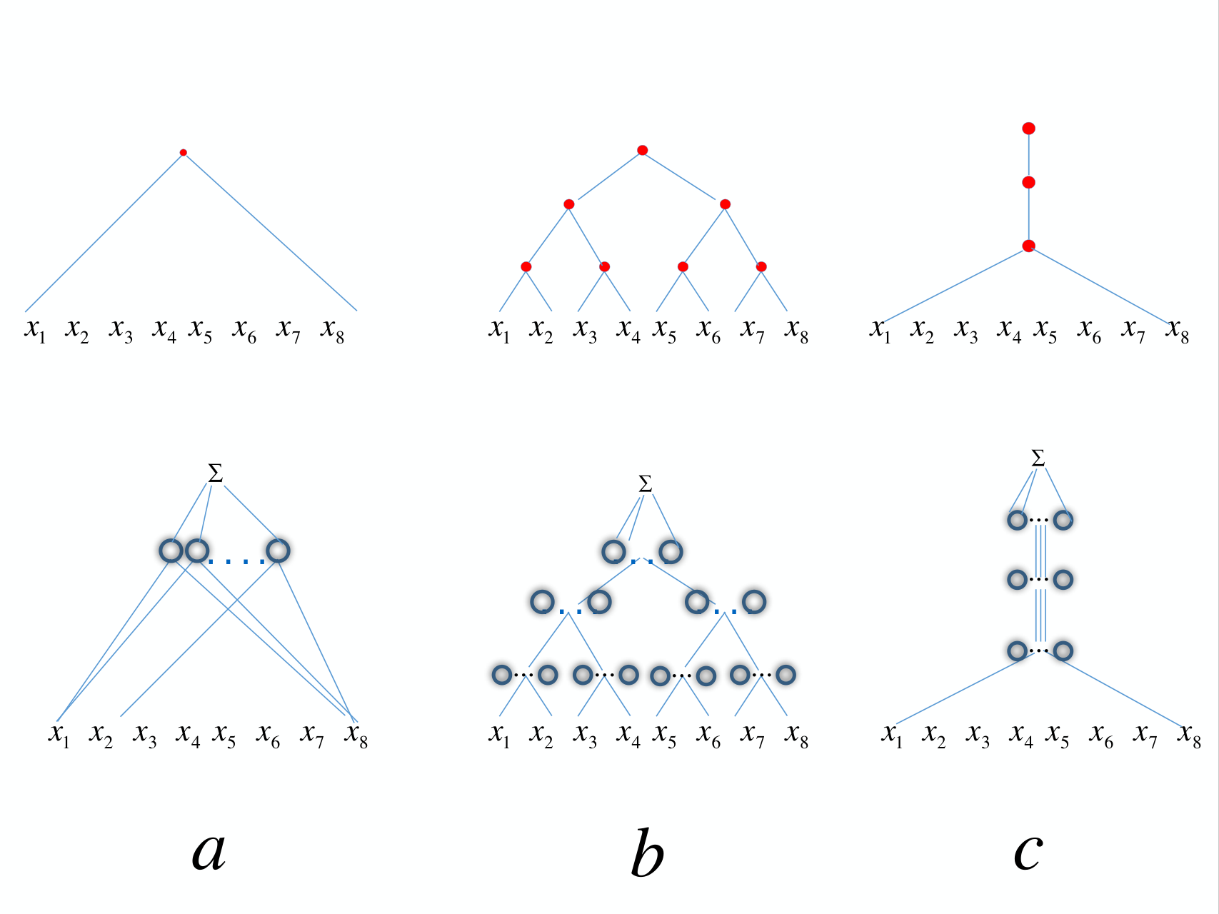
For example, if for some , then a network with complexity will be sufficient to guarantee an approximation with accuracy at least . Since is unknown, in order to obtain theoretically proved upper bounds, we need to make some assumptions on the class of functions from which the unknown target function is chosen. This a priori information is codified by the statement that for some subspace . This subspace is usually a smoothness class characterized by a smoothness parameter . Here it will be generalized to a smoothness and compositional class, characterized by the parameters and ( in the example of Figure 1; in general is the size of the kernel in a convolutional network).
3.2 Shallow and deep networks
This section characterizes conditions under which deep networks are “better” than shallow network in approximating functions. Thus we compare shallow (one-hidden layer) networks with deep networks as shown in Figure 1. Both types of networks use the same small set of operations – dot products, linear combinations, a fixed nonlinear function of one variable, possibly convolution and pooling. Each node in the networks we consider usually corresponds to a node in the graph of the function to be approximated, as shown in the Figure. In particular each node in the network contains a certain number of units. A unit is a neuron which computes
| (2) |
where is the vector of weights on the vector input . Both and the real number are parameters tuned by learning. We assume here that each node in the networks computes the linear combination of such units
| (3) |
Notice that for our main example of a deep network corresponding to a binary tree graph, the resulting architecture is an idealized version of the plethora of deep convolutional neural networks described in the literature. In particular, it has only one output at the top unlike most of the deep architectures with many channels and many top-level outputs. Correspondingly, each node computes a single value instead of multiple channels, using the combination of several units (see Equation 3). Our approach and basic results apply rather directly to more complex networks (see third note in section 6). A careful analysis and comparison with simulations will be described in future work.
The logic of our theorems is as follows.
- •
Both shallow (a) and deep (b) networks are universal, that is they can approximate arbitrarily well any continuous function of variables on a compact domain. The result for shallow networks is classical. Since shallow networks can be viewed as a special case of deep networks, it clear that for any continuous function of variables, there exists also a deep network that approximates the function arbitrarily well on a compact domain.
- •
We consider a special class of functions of variables on a compact domain that are a hierarchical compositions of local functions such as
(4) The structure of the function in equation 4 is represented by a graph of the binary tree type. This is the simplest example of compositional functions, reflecting dimensionality for the constituent functions . In general, is arbitrary but fixed and independent of the dimensionality of the compositional function . In our results we will often think of increasing while is fixed. In section 4 we will consider the more general compositional case.
- •
The approximation of functions with a compositional structure – can be achieved with the same degree of accuracy by deep and shallow networks but that the number of parameters are much smaller for the deep networks than for the shallow network with equivalent approximation accuracy. It is intuitive that a hierarchical network matching the structure of a compositional function should be “better” at approximating it than a generic shallow network but universality of shallow networks asks for non-obvious characterization of “better”. Our result makes clear that the intuition is indeed correct.
In the perspetive of machine learning, we assume that the shallow networks do not have any structural information on the function to be learned (here its compositional structure), because they cannot represent it directly and cannot exploit the advantage of a smaller number of parameters. In any case, in the context of approximation theory, we will exhibit and cite lower bounds of approximation by shallow networks for the class of compositional functions. Deep networks with standard architectures on the other hand do represent compositionality in their architecture and can be adapted to the details of such prior information.
We approximate functions of variables of the form of Equation (4) with networks in which the activation nonlinearity is a smoothed version of the so called ReLU, originally called ramp by Breiman and given by . The architecture of the deep networks reflects Equation (4) with each node being a ridge function, comprising one or more neurons.
Let , be the space of all continuous functions on , with . Let denote the class of all shallow networks with units of the form x↦∑_k=1^N a_kσ(⟨w_k,x⟩+b_k), where , . The number of trainable parameters here is . Let be an integer, and be the set of all functions of variables with continuous partial derivatives of orders up to such that , where denotes the partial derivative indicated by the multi-integer , and is the sum of the components of .
For the hierarchical binary tree network, the analogous spaces are defined by considering the compact set to be the class of all compositional functions of variables with a binary tree architecture and constituent functions in . We define the corresponding class of deep networks to be the set of all deep networks with a binary tree architecture, where each of the constituent nodes is in , where , being the set of non–leaf vertices of the tree. We note that in the case when is an integer power of , the total number of parameters involved in a deep network in – that is, weights and biases, is .
Two observations are critical to understand the meaning of our results:
- –
compositional functions of variables are a subset of functions of variables, that is . Deep networks can exploit in their architecture the special structure of compositional functions, whereas shallow networks are blind to it. Thus from the point of view of shallow networks, functions in are just functions in ; this is not the case for deep networks.
- –
the deep network does not need to have exactly the same compositional architecture as the compositional function to be approximated. It is sufficient that the acyclic graph representing the structure of the function is a subgraph of the graph representing the structure of the deep network. The degree of approximation estimates depend on the graph associated with the network and are thus an upper bound on what could be achieved by a network exactly matched to the function architecture.
The following two theorems estimate the degree of approximation for shallow and deep networks.
3.3 Shallow networks
The first theorem is about shallow networks.
Theorem 1.
Let be infinitely differentiable, and not a polynomial. For the complexity of shallow networks that provide accuracy at least is
(5) Notes In [27, Theorem 2.1], the theorem is stated under the condition that is infinitely differentiable, and there exists such that for any integer . It is proved in [28] that the second condition is equivalent to not being a polynomial. The proof in [27] relies on the fact that under these conditions on , the algebraic polynomials in variables of (total or coordinatewise) degree are in the uniform closure of the span of functions of the form (see Appendix 4.1). The estimate itself is an upper bound on the degree of approximation by such polynomials. Since it is based on the approximation of the polynomial space contained in the ridge functions implemented by shallow networks, one may ask whether it could be improved by using a different approach. The answer relies on the concept of nonlinear –width of the compact set (cf. [29, 4]). The n-width results imply that the estimate in Theorem (1) is the best possible among all reasonable [29] methods of approximating arbitrary functions in . The estimate of Theorem 1 is the best possible if the only a priori information we are allowed to assume is that the target function belongs to . The exponential dependence on the dimension of the number of parameters needed to obtain an accuracy is known as the curse of dimensionality. Note that the constants involved in in the theorems will depend upon the norms of the derivatives of as well as .
A simple but useful corollary follows from the proof of Theorem 1 about polynomials (which are a smaller space than spaces of Sobolev functions). Let us denote with the linear space of polynomials of degree at most in variables. Then
Corollary 1.
Let be infinitely differentiable, and not a polynomial. Every can be realized with an arbitrary accuracy by shallow network with units, .
3.4 Deep hierarchically local networks
Our second and main theorem is about deep networks with smooth activations and is recent (preliminary versions appeared in [3, 2, 4]). We formulate it in the binary tree case for simplicity but it extends immediately to functions that are compositions of constituent functions of a fixed number of variables instead than of variables as in the statement of the theorem (in convolutional networks corresponds to the size of the kernel).
Theorem 2.
For consider a deep network with the same compositonal architecture and with an activation function which is infinitely differentiable, and not a polynomial. The complexity of the network to provide approximation with accuracy at least is
(6) Proof To prove Theorem 2, we observe that each of the constituent functions being in , (1) applied with implies that each of these functions can be approximated from up to accuracy . Our assumption that implies that each of these constituent functions is Lipschitz continuous. Hence, it is easy to deduce that, for example, if , , are approximations to the constituent functions , , , respectively within an accuracy of , then since , and , then by Minkowski inequality. Thus
∥h(h_1,h_2)-P(P_1,P_2)∥ ≤cϵ, for some constant independent of the functions involved. This, together with the fact that there are nodes, leads to (6).
Also in this case the proof provides the following corollary about the subset of the space which consists of compositional polynomials with a binary tree graph and constituent polynomial functions of degree (in variables)
Corollary 2.
Let be infinitely differentiable, and not a polynomial. Let . Then can be realized by a deep network with a binary tree graph and a total of units with .
It is important to emphasize that the assumptions on in the theorems are not satisfied by the ReLU function , but they are satisfied by smoothing the function in an arbitrarily small interval around the origin. This suggests that the result of the theorem should be valid also for the non-smooth ReLU. Section 4.1 provides formal results. Stronger results than the theorems of this section (see [5]) hold for networks where each unit evaluates a Gaussian non–linearity; i.e., Gaussian networks of the form
(7) where the approximation is on the entire Euclidean space.
In summary, when the only a priori assumption on the target function is about the number of derivatives, then to guarantee an accuracy of , we need a shallow network with trainable parameters. If we assume a hierarchical structure on the target function as in Theorem 2, then the corresponding deep network yields a guaranteed accuracy of with trainable parameters. Note that Theorem 2 applies to all with a compositional architecture given by a graph which correspond to, or is a subgraph of, the graph associated with the deep network – in this case the graph corresponding to . Theorem 2 leads naturally to the notion of effective dimensionality that we formalize in the next section
Definition 1.
The effective dimension of a class of functions (for a given norm) is said to be if for every , any function in can be recovered within an accuracy of (as measured by the norm) using an appropriate network (either shallow or deep) with parameters.
Thus, the effective dimension for the class is , that of is .
4 General compositionality results: functions composed by a hierarchy of functions with bounded effective dimensionality
The main class of functions we considered in previous papers consists of functions as in Figure 1 b that we called compositional functions. The term “compositionality” was used with the meaning it has in language and vision, where higher level concepts are composed of a small number of lower level ones, objects are composed of parts, sentences are composed of words and words are composed of syllables. Notice that this meaning of compositionality is narrower than the mathematical meaning of composition of functions. The compositional functions we have described in previous papers may be more precisely called functions composed of hierarchically local functions.
Here we generalize formally our previous results to the broader class of compositional functions (beyond the hierarchical locality of Figure 1b to Figure 1c and Figure 2) by restating formally a few comments of previous papers. Let us begin with one of the previous examples. Consider
Since is nominally a polynomial of coordinatewise degree , [27, Lemma 3.2] shows that a shallow network with units is able to approximate arbitrarily well on . However, because of the hierarchical structure of , [27, Lemma 3.2] shows also that a hierarchical network with units can approximate the quadratic expression, and further layers, each with units can approximate the successive powers. Thus, a hierarchical network with layers and units can approximate arbitrarily well. We note that even if is nominally of degree , each of the monomial coefficients in is a function of only variables, .
A different example is
(8) This is obviously a Lipschitz continuous function of variables. The effective dimension of this class is , and hence, a shallow network would require at least parameters to approximate it within . However, the effective dimension of the class of univariate Lipschitz continuous functions is . Hence, if we take into account the fact that is a composition of a polynomial of degree in variables and the univariate Lipschitz continuous function , then it is easy to see that the same approximation can be achieved by using a two layered network with parameters.
To formulate our most general result that includes the examples above as well as the constraint of hierarchical locality, we first define formally a compositional function in terms of a directed acyclic graph. Let be a directed acyclic graph (DAG), with the set of nodes . A –function is defined as follows. Each of the source node obtains an input from . Each in-edge of every other node represents an input real variable, and the node itself represents a function of these input real variables, called a constituent function. The out-edges fan out the result of this evaluation. We assume that there is only one sink node, whose output is the -function. Thus, ignoring the compositionality of this function, it is a function of variables, where is the number of source nodes in .
Theorem 3.
Let be a DAG, be the number of source nodes, and for each , let be the number of in-edges of . Let be a compositional -function, where each of the constitutent function is in . Consider shallow and deep networks with infinitely smooth activation function as in Theorem 1. Then deep networks – with an associated graph that corresponds to the graph of – avoid the curse of dimensionality in approximating for increasing , whereas shallow networks cannot directly avoid the curse. In particular, the complexity of the best approximating shallow network is exponential in
(9) where , while the complexity of the deep network is
(10) Following definition 1 we call the effective dimension of function . Then, deep networks can avoid the curse of dimensionality if the constituent functions of a compositional function have a small effective dimension; i.e., have fixed, “small” dimensionality or fixed, “small” “roughness. A different interpretation of Theorem 3 is the following.
Proposition 1.
If a family of functions of smoothness has an effective dimension , then the functions are compositional in a manner consistent with the estimates in Theorem 3.
Notice that the functions included in this theorem are functions that are either local or the composition of simpler functions or both. Figure 2 shows some examples in addition to the examples at the top of Figure Figure 1.
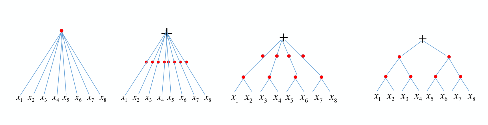
Figure 2: The figure shows the graphs of functions that may have small effective dimensionality, depending on the number of units per node required for good approximation. As before, there is a simple corollary for polynomial functions:
Corollary 3.
Let be infinitely differentiable, and not a polynomial. With the set up as in Theorem 3, let be DAG polynomial; i.e., a DAG function, each of whose constituent functions is a polynomial of degree . Then can be represented by a deep network with units, where is the number of non-leaf vertices, and is the maximal indegree of the nodes.
For example, if is a full binary tree with leaves, then the nominal degree of the polynomial as in Corollary 3 is , and therefore requires a shallow network with units, while a deep network requires only units.
Notice that polynomials in are sparse with a number of terms which is not exponential in , that is it is not but linear in (that is ) or at most polynomial in .
4.1 Approximation results for shallow and deep networks with (non-smooth) ReLUs
The results we described so far use smooth activation functions. We already mentioned why relaxing the smoothness assumption should not change our results in a fundamental way. While studies on the properties of neural networks with smooth activation abound, the results on non-smooth activation functions are much more sparse. Here we briefly recall some of them.
In the case of shallow networks, the condition of a smooth activation function can be relaxed to prove density (see [13], Proposition 3.7):
Proposition 2.
Let be in , and not a polynomial. Then shallow networks are dense in .
In particular, ridge functions using ReLUs of the form , with , are dense in .
Networks with non-smooth activation functions are expected to do relatively poorly in approximating smooth functions such as polynomials in the sup norm. “Good” degree of approximation rates (modulo a constant) have been proved in the norm. Define the unit ball in . Call the set of all continuous functions with continuous derivative up to degree defined on the unit ball. We define the Sobolev space as the completion of with respect to the Sobolev norm (see for details [13] page 168). We define the space and the approximation error . It is shown in [13, Corollary 6.10] that
Proposition 3.
For it holds for .
These approximation results with respect to the norm cannot be applied to derive bounds for compositional networks. Indeed, in the latter case, as we remarked already, estimates in the uniform norm are needed to control the propagation of the errors from one layer to the next, see Theorem 2. Results in this direction are given in [30], and more recently in [31] and [5] (see Theorem 3.1). In particular, using a result in [31] and following the proof strategy of Theorem 2 it is possible to derive the following results on the approximation of Lipshitz continuous functions with deep and shallow ReLU networks that mimics our Theorem 2:
Theorem 4.
Let be a -Lipshitz continuous function of variables. Then, the complexity of a network which is a linear combination of ReLU providing an approximation with accuracy at least is
wheres that of a deep compositional architecture is
Our general Theorem 3 can be extended in a similar way. Theorem 4 is an example of how the analysis of smooth activation functions can be adapted to ReLU. Indeed, it shows how deep compositional networks with standard ReLUs can avoid the curse of dimensionality. In the above results, the regularity of the function class is quantified by the magnitude of Lipshitz constant. Whether the latter is the best notion of smoothness for ReLU based networks, and if the above estimates can be improved, are interesting questions that we defer to a future work. A result that is more intuitive and may reflect what networks actually do is described in Appendix 4.3. Though the construction described there provides approximation in the norm but not in the sup norm, this is not a problem under any discretization of real number required for computer simulations (see Appendix).
Figures 3, 4, 5, 6 provide a sanity check and empirical support for our main results and for the claims in the introduction.
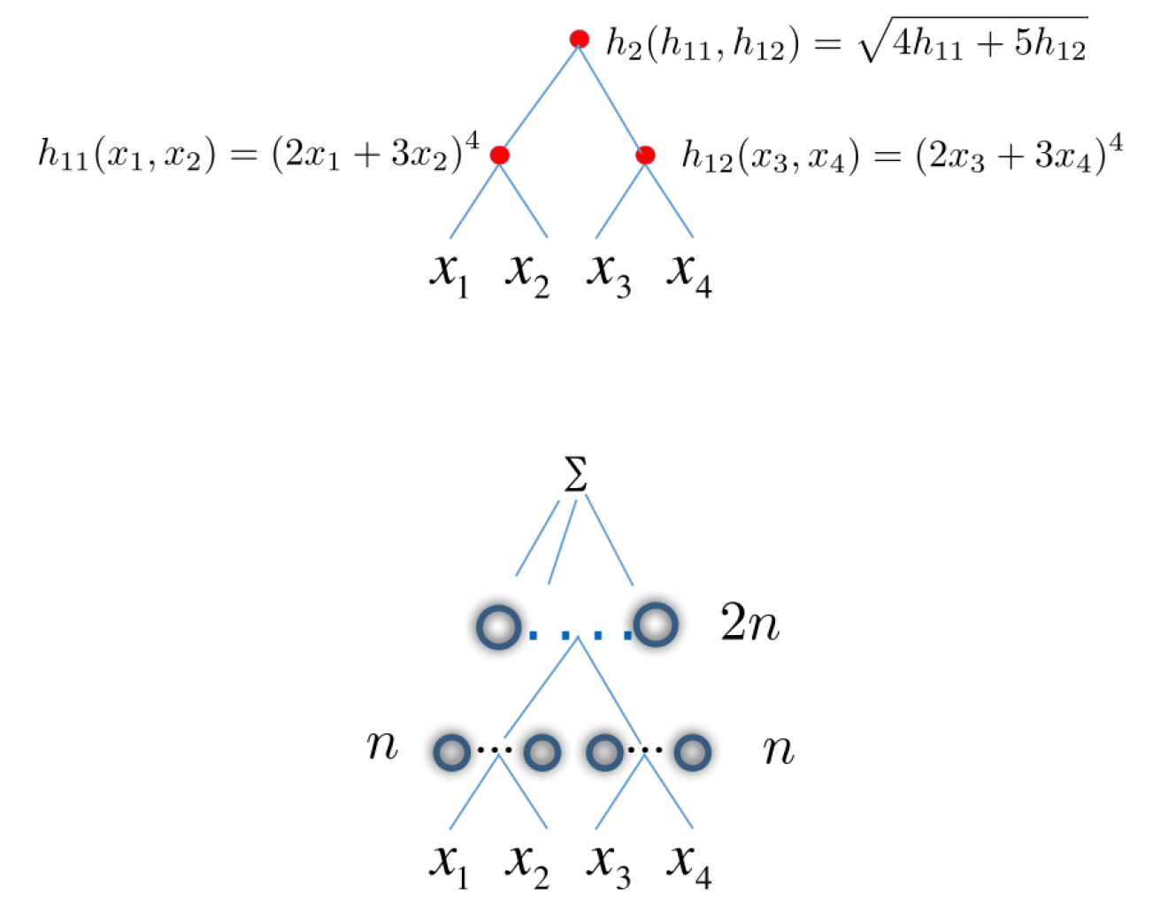
Figure 3: The figure shows on the top the graph of the function to be approximated, while the bottom part of the figure shows a deep neural network with the same graph structure. The left and right node inf the first layer has each units giving a total of units in the first layer. The second layer has a total of units. The first layer has a convolution of size to mirror the structure of the function to be learned. The compositional function we approximate has the form with , and as indicated in the figure. 
Figure 4: An empirical comparison of shallow vs 2-layers binary tree networks in the approximation of compositional functions. The loss function is the standard mean square error (MSE). There are several units per node of the tree. In our setup here the network with an associated binary tree graph was set up so that each layer had the same number of units and shared parameters. The number of units for the shallow and binary tree neural networks had the same number of parameters. On the left the function is composed of a single ReLU per node and is approximated by a network using ReLU activations. On the right the compositional function is and is approximated by a network with a smooth ReLU activation (also called softplus). The functions , , are as described in Figure 3. In order to be close to the function approximation case, a large data set of 60K training examples was used for both training sets. We used for SGD the Adam[32] optimizer. In order to get the best possible solution we ran 200 independent hyper parameter searches using random search [33] and reported the one with the lowest training error. The hyper parameters search was over the step size, the decay rate, frequency of decay and the mini-batch size. The exponential decay hyper parameters for Adam were fixed to the recommended values according to the original paper [32]. The implementations were based on TensorFlow [34]. 
Figure 5: Another comparison of shallow vs 2-layers binary tree networks in the learning of compositional functions. The set up of the experiment was the same as in the one in figure 4 except that the compositional function had two ReLU units per node instead of only one. The right part of the figure shows a cross section of the function in a bounded interval . The shape of the function is piecewise linear as it is always the case for ReLUs networks. Figure 6: We show that the main advantage of deep Convolutional Networks (ConvNets) comes from "hierarchical locality" instead of weight sharing. We train two 5-layer ConvNets with and without weight sharing on CIFAR-10. ConvNet without weight sharing has different filter parameters at each spatial location. There are 4 convolutional layers (filter size 3x3, stride 2) in each network. The number of feature maps (i.e., channels) are 16, 32, 64 and 128 respectively. There is an additional fully-connected layer as a classifier. The performances of a 2-layer and 5-layer fully-connected networks are also shown for comparison. Each hidden layer of the fully-connected network has 512 units. The models are all trained for 60 epochs with cross-entropy loss and standard shift and mirror flip data augmentation (during training). The training errors are higher than those of validation because of data augmentation. The learning rates are 0.1 for epoch 1 to 40, 0.01 for epoch 41 to 50 and 0.001 for rest epochs. The number of parameters for each model are indicated in the legends. Models with hierarchical locality significantly outperform shallow and hierarchical non-local networks. 4.2 Lower bounds and gaps
So far we have shown that there are deep networks – for instance of the convolutional type – that can avoid the curse of dimensionality if the functions they are learning are blessed with compositionality. There are no similar guarantee for shallow networks: for shallow networks approximating generic continuous functions the lower and the upper bound are both exponential[13]. From the point of view of machine learning, it is obvious that shallow networks, unlike deep ones, cannot exploit in their architecture the reduced number of parameters associated with priors corresponding to compositional functions. In past papers we listed a few examples, some of which are also valid lower bounds from the point of view of approximation theory:
- –
The polynomial considered earlier
can be approximated by deep networks with a smaller number of parameters than shallow networks is based on polynomial approximation of functions of the type . Here, however, a formal proof of the impossibility of good approximation by shallow networks is not available. For a lower bound we need at least one example of a compositional function which cannot be approximated by shallow networks with a non-exponential degree of approximation.
- –
Such an example, for which a proof of the lower bound exists since a few decades, consider a function which is a linear combination of tensor product Chui–Wang spline wavelets, where each wavelet is a tensor product cubic spline. It is shown in [11, 12] that is impossible to implement such a function using a shallow neural network with a sigmoidal activation function using neurons, but a deep network with the activation function can do so. In this case, as we mentioned, there is a formal proof of a gap between deep and shallow networks. Similarly, Eldan and Shamir [35] show other cases with separations that are exponential in the input dimension.
- –
As we mentioned earlier, Telgarsky proves an exponential gap between certain functions produced by deep networks and their approximation by shallow networks. The theorem [25] can be summarized as saying that a certain family of classification problems with real-valued inputs cannot be approximated well by shallow networks with fewer than exponentially many nodes whereas a deep network achieves zero error. This corresponds to high-frequency, sparse trigonometric polynomials in our case. His upper bound can be proved directly from our main theorem by considering the real-valued polynomials defined on the cube which is obviously a compositional function with a binary tree graph.
- –
We exhibit here another example to illustrate a limitation of shallow networks in approximating a compositional function.
Let be an integer, be the unit ball of . We consider the class of all compositional functions , where , and , and . We consider
where is either the class of all shallow networks with units or of deep networks with two layers, the first with inputs, and the next with one input. The both cases, the activation function is a function that is not a polynomial.
Theorem 5.
There exist constants such that for ,
(11) In contrast, there exists such that
(12) The constants may depend upon .
Proof. The estimate (12) follows from the estimates already given for deep networks. To prove (11), we use Lemma 3.2 in [12]. Let be a function supported on , and we consider . We may clearly choose so that . Then it is clear that each . Clearly,
(13) We choose such that
(14) Since is supported on , we may imitate the proof of Lemma 3.2 in [12] with . Let be such that (without loss of generality) , and be the Dirac measure supported at . We group in disjoint groups of vectors each. For each group, we take vectors such that is orthogonal to the ’s in group . The argument in the proof of Lemma 3.2 in [12] can be modified to get a measure with total variation such that
It is easy to deduce from here as in [12] using the duality principle that
So by now plenty of examples of lower bounds exist showing a gap between shallow and deep networks. A particularly interesting case is the product function, that is the monomial which is, from our point of view, the prototypical compositional functions. Keeping in mind the issue of lower bounds, the question here has to do with the minimum integer such that the function is in the closure of the span of , with , and , ranging over their whole domains. Such a result has been claimed for the case of smooth ReLUs, using unusual group techniques and is sketched in the Appendix of [36].
Notice, in support of the conjecture, that assuming that a shallow network with (non-smooth) ReLUs has a lower bound of will lead to an apparent contradiction with Hastad theorem (which is about representation not approximation of Boolean functions) by restricting from to . Hastad theorem [37] establishes the inapproximability of the parity function by shallow circuits of non-exponential size.
4.3 Messy graphs and densely connected deep networks
As mentioned already, the approximating deep network does not need to exactly match the architecture of the compositional function as long as the graph or tree associated with the function is contained in the graph associated with the network. This is of course good news: the compositionality prior embedded in the architecture of the network does not to reflect exactly the graph of a new function to be learned. We have shown that for a given class of compositional functions characterized by an associated graph there exist a deep network that approximates such a function better than a shallow network. The same network approximates well functions characterized by subgraphs of the original class.
The proofs of our theorems show that linear combinations of compositional functions are universal in the sense that they can approximate any function and that deep networks with a number of units that increases exponentially with layers can approximate any function. Notice that deep compositional networks can interpolate if they are overparametrized with respect to the data, even if the data reflect a non-compositional function.
As an aside, note that the simplest compositional function – addition – is trivial in the sense that it offers no approximation advantage to deep networks. The key function is multiplication which is for us the prototypical compositional functions. As a consequence, polynomial functions are compositional – they are linear combinations of monomials which are compositional. However, their compositional structure does not confer any advantage in terms of approximation, because of the exponential number of compositional terms.
As we mentioned earlier, networks corresponding to graphs that include the graph of the function to be learned can exploit compositionality. The relevant number of parameters to be optimized, however, is the number of parameters in the network and not the number of parameters () of the optimal deep network with a graph exactly matched to the graph of the function to be learned. As an aside, the price to be paid in using a non-optimal prior depend on the learning algorithm. For instance, under sparsity constraints it may be possible to pay a smaller price than (but higher than ).
In this sense, some of the densely connected deep networks used in practice – which contain sparse graphs possibly relevant for the function to be learned and which are still “smaller” than the exponential number of units required to represent a generic function of variables – may be capable in some cases of exploiting an underlying compositionality structure without paying an exhorbitant price in terms of required complexity.
5 Connections with the theory of Boolean functions
The approach followed in our main theorems suggest the following considerations (see Appendix 1 for a brief introduction). The structure of a deep network is reflected in polynomials that are best approximated by it – for instance generic polynomials or sparse polynomials (in the coefficients) in variables of order . The tree structure of the nodes of a deep network reflects the structure of a specific sparse polynomial. Generic polynomial of degree in variables are difficult to learn because the number of terms, trainable parameters and associated VC-dimension are all exponential in . On the other hand, functions approximated well by sparse polynomials can be learned efficiently by deep networks with a tree structure that matches the polynomial. We recall that in a similar way several properties of certain Boolean functions can be “read out” from the terms of their Fourier expansion corresponding to “large” coefficients, that is from a polynomial that approximates well the function.
Classical results [37] about the depth-breadth tradeoff in circuits design show that deep circuits are more efficient in representing certain Boolean functions than shallow circuits. Hastad proved that highly-variable functions (in the sense of having high frequencies in their Fourier spectrum), in particular the parity function cannot even be decently approximated by small constant depth circuits (see also [38]). A closely related result follow immediately from our main theorem since functions of real variables of the form have the compositional form of the binary tree (for even). Restricting the values of the variables to yields an upper bound:
Proposition 4.
The family of parity functions with and can be represented with exponentially fewer units by a deep than a shallow network.
Notice that Hastad’s results on Boolean functions have been often quoted in support of the claim that deep neural networks can represent functions that shallow networks cannot. For instance Bengio and LeCun [39] write “We claim that most functions that can be represented compactly by deep architectures cannot be represented by a compact shallow architecture”.”.
Finally, we want to mention a few other observations on Boolean functions that shows an interesting connection with our approach. It is known that within Boolean functions the class of polynomial size constant depth circuits is characterized by Fourier transforms where most of the power spectrum is in the low order coefficients. Such functions can be approximated well by a polynomial of low degree and can be learned well by considering only such coefficients. There are two algorithms [40] that allow learning of certain Boolean function classes:
- 1.
the low order algorithm that approximates functions by considering their low order Fourier coefficients and
- 2.
the sparse algorithm which learns a function by approximating its significant coefficients.
Decision lists and decision trees can be learned by the first algorithm. Functions with small norm can be approximated well by the second algorithm. Boolean circuits expressing DNFs can be approximated by the first one but even better by the second. In fact, in many cases a function can be approximated by a small set of coefficients but these coefficients do not correspond to low-order terms. All these cases are consistent with the notes about sparse functions in section 6.
6 Notes on a theory of compositional computation
The key property of the theory of compositional functions sketched here is that certain deep networks can learn them avoiding the curse of dimensionality because of the blessing of compositionality via a small effective dimension.
We state here several comments and conjectures.
- 1.
General comments
- –
Assumptions of the compositionality type may have more direct practical implications and be at least as effective as assumptions about function smoothness in countering the curse of dimensionality in learning and approximation.
- –
- –
The main question that may be asked about the relevance of the theoretical results of this paper and networks used in practice has to do with the many “channels” used in the latter and with our assumption that each node in the networks computes a scalar function – the linear combination of units (Equation 3). The following obvious but interesting extension of Theorem 1 to vector-valued functions says that the number of hidden units required for a given accuracy in each component of the function is the same as in the scalar case considered in our theorems (of course the number of weigths is larger):
Corollary 4.
Let be infinitely differentiable, and not a polynomial. For a vector-valued function with components the number of hidden units in shallow networks with inputs, outputs that provide accuracy at least in each of the components of is
(15) The demonstration follows the proof of theorem 1, see also Appendix 4.1. It amounts to realizing that the hidden units (or linear combinations of them) can be equivalent to the monomials of a generic polynomial of degree in variables that can be used by a different set of coefficients for each of the . This argument of course does not mean that during learning this is what happens; it provides one way to perform the approximation and an associated upper bound. The corollary above leads to a simple argument that generalizes our binary tree results to standard, multi-channel deep convolutional networks by introducing a set of virtual linear units as ouputs of one layer and inputs of the next one. This in turn leads to the following prediction: for consistent approximation accuracy across the layers, the rank of the weights matrices between units in successive layers should have a rank in the order of the number of the dimensionality in the first layer (inputs and outputs have to be defined wrt support of the convolution kernel). This suggests rank-deficient weight matrices in present networks.
- –
We have used polynomials (but see Appendix 4.3) to prove results about complexity of approximation in the case of neural networks. Neural network learning with SGD may or may not synthesize polynomial, depending on the smoothness of the activation function and on the target. This is not a problem for theoretically establishing upper bounds on the degree of convergence because results using the framework on nonlinear width guarantee the “polynomial” bounds are optimal.
- –
Both shallow and deep representations may or may not reflect invariance to group transformations of the inputs of the function ([41, 22]). Invariance – also called weight sharing – decreases the complexity of the network. Since we are interested in the comparison of shallow vs deep architectures, we have considered the generic case of networks (and functions) for which invariance is not assumed. In fact, the key advantage of deep vs. shallow network – as shown by the proof of the theorem – is the associated hierarchical locality (the constituent functions in each node are local that is have a small dimensionality) and not invariance (which designates shared weights that is nodes at the same level sharing the same function). One may then ask about the relation of these results with i-theory[42]. The original core of i-theory describes how pooling can provide either shallow or deep networks with invariance and selectivity properties. Invariance of course helps but not exponentially as hierarchical locality does.
- –
There are several properties that follow from the theory here which are attractive from the point of view of neuroscience. A main one is the robustness of the results with respect to the choice of nonlinearities (linear rectifiers, sigmoids, Gaussians etc.) and pooling.
- –
In a machine learning context, minimization over a training set of a loss function such as the square loss yields an empirical approximation of the regression function . Our hypothesis of compositionality becomes an hypothesis about the structure of the conditional probability function.
- –
- 2.
Spline approximations, Boolean functions and tensors
- –
Consider again the case of section 4 of a multivariate function . Suppose to discretize it by a set of piecewise constant splines and their tensor products. Each coordinate is effectively replaced by boolean variables.This results in a -dimensional table with entries. This in turn corresponds to a boolean function . Here, the assumption of compositionality corresponds to compressibility of a -dimensional table in terms of a hierarchy of -dimensional tables. Instead of entries there are entries. This has in turn obvious connections with HVQ (Hierarchical Vector Quantization), discussed in Appendix 5.
- –
As Appendix 4.3 shows, every function can be approximated by an epsilon-close binary function . Binarization of is done by using partitions for each variable and indicator functions. Thus and , with depending on and bounded .
- –
can be written as a polynomial (a Walsh decomposition) . It is always possible to associate a to any , given .
- –
The binarization argument suggests a direct way to connect results on function approximation by neural nets with older results on Boolean functions. The latter are special cases of the former results.
- –
One can think about tensors in terms of -dimensional tables. The framework of hierarchical decompositions of tensors – in particular the Hierarchical Tucker format – is closely connected to our notion of compositionality. Interestingly, the hierarchical Tucker decomposition has been the subject of recent papers on Deep Learning (for instance see [20]). This work, as well more classical papers [43], does not characterize directly the class of functions for which these decompositions are effective. Notice that tensor decompositions assume that the sum of polynomial functions of order is sparse (see eq. at top of page 2030 of [43]). Our results provide a rigorous grounding for the tensor work related to deep learning. There is obviously a wealth of interesting connections with approximation theory that should be explored.
Notice that the notion of separation rank of a tensor is very closely related to the effective in Equation 26.
- –
- 3.
Sparsity
- –
We suggest to define binary sparsity of , in terms of the sparsity of the boolean function ; binary sparsity implies that an approximation to can be learned by non-exponential deep networks via binarization. Notice that if the function is compositional the associated Boolean functions is sparse; the converse is not true.
- –
In may situations, Tikhonov regularization corresponds to cutting high order Fourier coefficients. Sparsity of the coefficients subsumes Tikhonov regularization in the case of a Fourier representation. Notice that as an effect the number of Fourier coefficients is reduced, that is trainable parameters, in the approximating trigonometric polynomial. Sparsity of Fourier coefficients is a general constraint for learning Boolean functions.
- –
Sparsity in a specific basis. A set of functions may be defined to be sparse in a specific basis when the number of parameters necessary for its -approximation increases less than exponentially with the dimensionality. An open question is the appropriate definition of sparsity. The notion of sparsity we suggest here is the effective in Equation 26. For a general function ; we may define sparse functions those for which in
(16) where is a specific polynomial that approximates within the desired . Notice that the polynomial can be a sum of monomials or a sum of, for instance, orthogonal polynomials with a total of parameters. In general, sparsity depends on the basis and one needs to know the basis and the type of sparsity to exploit it in learning, for instance with a deep network with appropriate activation functions and architecture.
There are function classes that are sparse in every bases. Examples are compositional functions described by a binary tree graph.
- –
- 4.
The role of compositionality in generalization by multi-class deep networks
Most of the succesfull neural networks exploit compositionality for better generalization in an additional important way (see [44]). Suppose that the mappings to be learned in a family of classification tasks (for instance classification of different object classes in Imagenet) may be approximated by compositional functions such as , where depends on the task (for instance to which object class) but all the other constituent functions are common across the tasks. Under such an assumption, multi-task learning, that is training simultaneously for the different tasks, forces the deep network to “find” common constituent functions. Multi-task learning has theoretical advantages that depends on compositionality: the sample complexity of the problem can be significantly lower (see [45]). The Maurer’s approach is in fact to consider the overall function as the composition of a preprocessor function common to all task followed by a task-specific function. As a consequence, the generalization error, defined as the difference between expected and empirical error, averaged across the tasks, is bounded with probability at least (in the case of finite hypothesis spaces) by
(17) where is the size of the training set, is the hypothesis space of the common classifier and is the hypothesis space of the system of constituent functions, common across tasks.
The improvement in generalization error because of the multitask structure can be in the order of the square root of the number of tasks (in the case of Imagenet with its object classes the generalization error may tyherefore decrease bt a factor ). It is important to emphasize the dual advantage here of compositionality, which a) reduces generalization error by decreasing the complexity of the hypothesis space of compositional functions relative the space of non-compositional functions and b) exploits the multi task structure, that replaces with .
We conjecture that the good generalization exhibited by deep convolutional networks in multi-class tasks such as CiFAR and Imagenet are due to three factors:
- –
the regularizing effect of SGD
- –
the task is compositional
- –
the task is multiclass.
- –
- 5.
Deep Networks as memories
Notice that independently of considerations of generalization, deep compositional networks are expected to be very efficient memories – in the spirit of hierarchical vector quantization – for associative memories reflecting compositional rules (see Appendix 5 and [46]). Notice that the advantage with respect to shallow networks from the point of view of memory capacity can be exponential (as in the example after Equation 32 showing ).
- 6.
Theory of computation, locality and compositionality
- –
From the computer science point of view, feedforward multilayer networks are equivalent to finite state machines running for a finite number of time steps[47, 48]. This result holds for almost any fixed nonlinearity in each layer. Feedforward networks are equivalent to cascades without loops (with a finite number of stages) and all other forms of loop free cascades (i.e. McCulloch-Pitts nets without loops, perceptrons, analog perceptrons, linear threshold machines). Finite state machines, cascades with loops, and difference equation systems which are Turing equivalent, are more powerful than multilayer architectures with a finite number of layers. The latter networks, however, are practically universal computers, since every machine we can build can be approximated as closely as we like by defining sufficiently many stages or a sufficiently complex single stage. Recurrent networks as well as differential equations are Turing universal.
In other words, all computable functions (by a Turing machine) are recursive, that is composed of a small set of primitive operations. In this broad sense all computable functions are compositional (composed from elementary functions). Conversely a Turing machine can be written as a compositional function where , being parameters that are inputs and outputs of . If is bounded we have a finite state machine, otherwise a Turing machine. in terms of elementary functions. As mentioned above, each layer in a deep network correspond to one time step in a Turing machine. In a sense, this is sequential compositionality, as in the example of Figure 1 c. The hierarchically local compositionality we have introduced in this paper has the flavour of compositionality in space.
Of course, since any function can be approximated by polynomials, and a polynomial can always be calculated using a recursive procedure and a recursive procedure can always be unwound as a “deep network”, any function can always be approximated by a compositional function of a few variables. However, generic compositionality of this type does not guarantee good approximation properties by deep networks.
- –
Hierarchically local compositionality can be related to the notion of local connectivity of a network. Connectivity is a key property in network computations. Local processing may be a key constraint also in neuroscience. One of the natural measures of connectivity that can be introduced is the order of a node defined as the number of its distinct inputs. The order of a network is then the maximum order among its nodes. The term order dates back to the Perceptron book ([49], see also [48]). From the previous observations, it follows that a hierarchical network of order at least can be universal. In the Perceptron book many interesting visual computations have low order (e.g. recognition of isolated figures). The message is that they can be implemented in a single layer by units that have a small number of inputs. More complex visual computations require inputs from the full visual field. A hierarchical network can achieve effective high order at the top using units with low order. The network architecture of Figure 1 b) has low order: each node in the intermediate layers is connected to just 2 other nodes, rather than (say) all nodes in the previous layer (notice that the connections in the trees of the figures may reflect linear combinations of the input units).
- –
Low order may be a key constraint for cortex. If it captures what is possible in terms of connectivity between neurons, it may determine by itself the hierarchical architecture of cortex which in turn may impose compositionality to language and speech.
- –
The idea of functions that are compositions of “simpler” functions extends in a natural way to recurrent computations and recursive functions. For instance represents iterations of the algorithm ( and match input and output dimensions to ).
- –
7 Why are compositional functions so common?
Let us provide a couple of simple examples of compositional functions. Addition is compositional but the degree of approximation does not improve by decomposing addition in different layers of a network; all linear operators are compositional with no advantage for deep networks; multiplication as well as the AND operation (for Boolean variables) is the prototypical compositional function that provides an advantage to deep networks. So compositionality is not enough: we need certain sublasses of compositional functions (such as the hierarchically local functions we described) in order to avoid the curse of dimensionality.
It is not clear, of course, why problems encountered in practice should match this class of functions. Though we and others have argued that the explanation may be in either the physics or the neuroscience of the brain, these arguments (see Appendix 2) are not (yet) rigorous. Our conjecture at present is that compositionality is imposed by the wiring of our cortex and is reflected in language and the common problems we worry about. Thus compositionality of several – but not all – computations on images many reflect the way we describe and think about them.
Acknowledgment
This work was supported by the Center for Brains, Minds and Machines (CBMM), funded by NSF STC award CCF – 1231216. HNM was supported in part by ARO Grant W911NF-15-1-0385. We thank O. Shamir for useful emails that prompted us to clarify our results in the context of lower bounds and for pointing out a number of typos and other mistakes.
References
- [1] F. Anselmi, L. Rosasco, C. Tan, and T. Poggio, “Deep convolutional network are hierarchical kernel machines,” Center for Brains, Minds and Machines (CBMM) Memo No. 35, also in arXiv, 2015.
- [2] T. Poggio, L. Rosasco, A. Shashua, N. Cohen, and F. Anselmi, “Notes on hierarchical splines, dclns and i-theory,” tech. rep., MIT Computer Science and Artificial Intelligence Laboratory, 2015.
- [3] T. Poggio, F. Anselmi, and L. Rosasco, “I-theory on depth vs width: hierarchical function composition,” CBMM memo 041, 2015.
- [4] H. Mhaskar, Q. Liao, and T. Poggio, “Learning real and boolean functions: When is deep better than shallow?,” Center for Brains, Minds and Machines (CBMM) Memo No. 45, also in arXiv, 2016.
- [5] H. Mhaskar and T. Poggio, “Deep versus shallow networks: an approximation theory perspective,” Center for Brains, Minds and Machines (CBMM) Memo No. 54, also in arXiv, 2016.
- [6] D. L. Donoho, “High-dimensional data analysis: The curses and blessings of dimensionality,” in AMS CONFERENCE ON MATH CHALLENGES OF THE 21ST CENTURY, 2000.
- [7] Y. LeCun, Y. Bengio, and H. G., “Deep learning,” Nature, pp. 436–444, 2015.
- [8] K. Fukushima, “Neocognitron: A self-organizing neural network for a mechanism of pattern recognition unaffected by shift in position,” Biological Cybernetics, vol. 36, no. 4, pp. 193–202, 1980.
- [9] M. Riesenhuber and T. Poggio, “Hierarchical models of object recognition in cortex,” Nature Neuroscience, vol. 2, pp. 1019–1025, Nov. 1999.
- [10] H. Mhaskar, “Approximation properties of a multilayered feedforward artificial neural network,” Advances in Computational Mathematics, pp. 61–80, 1993.
- [11] C. Chui, X. Li, and H. Mhaskar, “Neural networks for localized approximation,” Mathematics of Computation, vol. 63, no. 208, pp. 607–623, 1994.
- [12] C. K. Chui, X. Li, and H. N. Mhaskar, “Limitations of the approximation capabilities of neural networks with one hidden layer,” Advances in Computational Mathematics, vol. 5, no. 1, pp. 233–243, 1996.
- [13] A. Pinkus, “Approximation theory of the mlp model in neural networks,” Acta Numerica, vol. 8, pp. 143–195, 1999.
- [14] T. Poggio and S. Smale, “The mathematics of learning: Dealing with data,” Notices of the American Mathematical Society (AMS), vol. 50, no. 5, pp. 537–544, 2003.
- [15] B. B. Moore and T. Poggio, “Representations properties of multilayer feedforward networks,” Abstracts of the First annual INNS meeting, vol. 320, p. 502, 1998.
- [16] R. Livni, S. Shalev-Shwartz, and O. Shamir, “A provably efficient algorithm for training deep networks,” CoRR, vol. abs/1304.7045, 2013.
- [17] O. Delalleau and Y. Bengio, “Shallow vs. deep sum-product networks,” in Advances in Neural Information Processing Systems 24: 25th Annual Conference on Neural Information Processing Systems 2011. Proceedings of a meeting held 12-14 December 2011, Granada, Spain., pp. 666–674, 2011.
- [18] R. Montufar, G. F.and Pascanu, K. Cho, and Y. Bengio, “On the number of linear regions of deep neural networks,” Advances in Neural Information Processing Systems, vol. 27, pp. 2924–2932, 2014.
- [19] H. N. Mhaskar, “Neural networks for localized approximation of real functions,” in Neural Networks for Processing [1993] III. Proceedings of the 1993 IEEE-SP Workshop, pp. 190–196, IEEE, 1993.
- [20] N. Cohen, O. Sharir, and A. Shashua, “On the expressive power of deep learning: a tensor analysis,” CoRR, vol. abs/1509.0500, 2015.
- [21] F. Anselmi, J. Leibo, L. Rosasco, J. Mutch, A. Tacchetti, and T. Poggio, “Unsupervised learning of invariant representations with low sample complexity: the magic of sensory cortex or a new framework for machine learning?.,” Center for Brains, Minds and Machines (CBMM) Memo No. 1. arXiv:1311.4158v5, 2014.
- [22] F. Anselmi, J. Z. Leibo, L. Rosasco, J. Mutch, A. Tacchetti, and T. Poggio, “Unsupervised learning of invariant representations,” Theoretical Computer Science, 2015.
- [23] T. Poggio, L. Rosaco, A. Shashua, N. Cohen, and F. Anselmi, “Notes on hierarchical splines, dclns and i-theory,” CBMM memo 037, 2015.
- [24] Q. Liao and T. Poggio, “Bridging the gap between residual learning, recurrent neural networks and visual cortex,” Center for Brains, Minds and Machines (CBMM) Memo No. 47, also in arXiv, 2016.
- [25] M. Telgarsky, “Representation benefits of deep feedforward networks,” arXiv preprint arXiv:1509.08101v2 [cs.LG] 29 Sep 2015, 2015.
- [26] I. Safran and O. Shamir, “Depth separation in relu networks for approximating smooth non-linear functions,” arXiv:1610.09887v1, 2016.
- [27] H. N. Mhaskar, “Neural networks for optimal approximation of smooth and analytic functions,” Neural Computation, vol. 8, no. 1, pp. 164–177, 1996.
- [28] E. Corominas and F. S. Balaguer, “Condiciones para que una funcion infinitamente derivable sea un polinomio,” Revista matemática hispanoamericana, vol. 14, no. 1, pp. 26–43, 1954.
- [29] R. A. DeVore, R. Howard, and C. A. Micchelli, “Optimal nonlinear approximation,” Manuscripta mathematica, vol. 63, no. 4, pp. 469–478, 1989.
- [30] H. N. Mhaskar, “On the tractability of multivariate integration and approximation by neural networks,” J. Complex., vol. 20, pp. 561–590, Aug. 2004.
- [31] F. Bach, “Breaking the curse of dimensionality with convex neural networks,” arXiv:1412.8690, 2014.
- [32] D. P. Kingma and J. Ba, “Adam: A method for stochastic optimization,” CoRR, vol. abs/1412.6980, 2014.
- [33] J. Bergstra and Y. Bengio, “Random search for hyper-parameter optimization,” J. Mach. Learn. Res., vol. 13, pp. 281–305, Feb. 2012.
- [34] M. Abadi, A. Agarwal, P. Barham, E. Brevdo, Z. Chen, C. Citro, G. S. Corrado, A. Davis, J. Dean, M. Devin, S. Ghemawat, I. Goodfellow, A. Harp, G. Irving, M. Isard, Y. Jia, R. Jozefowicz, L. Kaiser, M. Kudlur, J. Levenberg, D. Mané, R. Monga, S. Moore, D. Murray, C. Olah, M. Schuster, J. Shlens, B. Steiner, I. Sutskever, K. Talwar, P. Tucker, V. Vanhoucke, V. Vasudevan, F. Viégas, O. Vinyals, P. Warden, M. Wattenberg, M. Wicke, Y. Yu, and X. Zheng, “TensorFlow: Large-scale machine learning on heterogeneous systems,” 2015. Software available from tensorflow.org.
- [35] R. Eldan and O. Shamir, “The power of depth for feedforward neural networks,” arXiv preprint arXiv:1512.03965v4, 2016.
- [36] M. Lin, H.and Tegmark, “Why does deep and cheap learning work so well?,” arXiv:1608.08225, pp. 1–14, 2016.
- [37] J. T. Hastad, Computational Limitations for Small Depth Circuits. MIT Press, 1987.
- [38] N. Linial, M. Y., and N. N., “Constant depth circuits, fourier transform, and learnability,” Journal of the ACM, vol. 40, no. 3, p. 607–620, 1993.
- [39] Y. Bengio and Y. LeCun, “Scaling learning algorithms towards ai,” in Large-Scale Kernel Machines (L. Bottou, O. Chapelle, and J. DeCoste, D.and Weston, eds.), MIT Press, 2007.
- [40] Y. Mansour, “Learning boolean functions via the fourier transform,” in Theoretical Advances in Neural Computation and Learning (V. Roychowdhury, K. Siu, and A. Orlitsky, eds.), pp. 391–424, Springer US, 1994.
- [41] S. Soatto, “Steps Towards a Theory of Visual Information: Active Perception, Signal-to-Symbol Conversion and the Interplay Between Sensing and Control,” arXiv:1110.2053, pp. 0–151, 2011.
- [42] F. Anselmi and T. Poggio, Visual Cortex and Deep Networks. MIT Press, 2016.
- [43] L. Grasedyck, “Hierarchical Singular Value Decomposition of Tensors,” SIAM J. Matrix Anal. Appl., no. 31,4, pp. 2029–2054, 2010.
- [44] B. M. Lake, R. Salakhutdinov, and J. B. Tenenabum, “Human-level concept learning through probabilistic program induction,” Science, vol. 350, no. 6266, pp. 1332–1338, 2015.
- [45] A. Maurer, “Bounds for Linear Multi-Task Learning,” Journal of Machine Learning Research, 2015.
- [46] F. Anselmi, L. Rosasco, and T. Tan, C.and Poggio, “Deep Convolutional Networks are Hierarchical Kernel Machines,” Center for Brains, Minds and Machines (CBMM) Memo No. 35, also in arXiv, 2015.
- [47] S. Shalev-Shwartz and S. Ben-David, Understanding Machine Learning: From Theory to Algorithms. Cambridge eBooks, 2014.
- [48] T. Poggio and W. Reichardt, “On the representation of multi-input systems: Computational properties of polynomial algorithms.,” Biological Cybernetics, 37, 3, 167-186., 1980.
- [49] M. Minsky and S. Papert, Perceptrons: An Introduction to Computational Geometry. Cambridge MA: The MIT Press, ISBN 0-262-63022-2, 1972.
- [50] D. Ruderman, “Origins of scaling in natural images,” Vision Res., pp. 3385 – 3398, 1997.
- [51] F. Girosi, M. Jones, and T. Poggio, “Regularization theory and neural networks architectures,” Neural Computation, vol. 7, pp. 219–269, 1995.
- [52] T. Poggio and F. Girosi, “A theory of networks for approximation and learning,” Laboratory, Massachusetts Institute of Technology, vol. A.I. memo n1140, 1989.
- [53] J. Mihalik, “Hierarchical vector quantization. of images in transform domain.,” ELEKTROTECHN. CA5, 43, NO. 3. 92,94., 1992.
- [54] F. Girosi and T. Poggio, “Representation properties of networks: Kolmogorov’s theorem is irrelevant,” Neural Computation, vol. 1, no. 4, pp. 465–469, 1989.
- [55] F. Girosi and T. Poggio, “Networks and the best approximation property,” Biological Cybernetics, vol. 63, pp. 169–176, 1990.
- [56] M. Anthony and P. Bartlett, Neural Network Learning - Theoretical Foundations. Cambridge University Press, 2002.
Appendix: observations, theorems and conjectures
1 Boolean Functions
One of the most important tools for theoretical computer scientists for the study of functions of Boolean variables, their related circuit design and several associated learning problems, is the Fourier transform over the Abelian group . This is known as Fourier analysis over the Boolean cube . The Fourier expansion of a Boolean function or even a real-valued Boolean function is its representation as a real polynomial, which is multilinear because of the Boolean nature of its variables. Thus for Boolean functions their Fourier representation is identical to their polynomial representation. In this paper we use the two terms interchangeably. Unlike functions of real variables, the full finite Fourier expansion is exact, instead of an approximation. There is no need to distingush between trigonometric and real polynomials. Most of the properties of standard harmonic analysis are otherwise preserved, including Parseval theorem. The terms in the expansion correspond to the various monomials; the low order ones are parity functions over small subsets of the variables and correspond to low degrees and low frequencies in the case of polynomial and Fourier approximations, respectively, for functions of real variables.
2 Does Physics or Neuroscience imply compositionality?
It has been often argued that not only text and speech are compositional but so are images. There are many phenomena in nature that have descriptions along a range of rather different scales. An extreme case consists of fractals which are infinitely self-similar, iterated mathematical constructs. As a reminder, a self-similar object is similar to a part of itself (i.e. the whole is similar to one or more of the parts). Many objects in the real world are statistically self-similar, showing the same statistical properties at many scales: clouds, river networks, snow flakes, crystals and neurons branching. A relevant point is that the shift-invariant scalability of image statistics follows from the fact that objects contain smaller clusters of similar surfaces in a selfsimilar fractal way. Ruderman [50] analysis shows that image statistics reflects what has been known as the property of compositionality of objects and parts: parts are themselves objects, that is selfsimilar clusters of similar surfaces in the physical world. Notice however that, from the point of view of this paper, it is misleading to say that an image is compositional: in our terminology a function on an image may be compositional but not its argument. In fact, functions to be learned may or may not be compositional even if their input is an image since they depend on the input but also on the task (in the supervised case of deep learning networks all weights depend on and ). Conversely, a network may be given a function which can be written in a compositional form, independently of the nature of the input vector such as the function “multiplication of all scalar inputs’ components”. Thus a more reasonable statement is that “many natural questions on images correspond to algorithms which are compositional”. Why this is the case is an interesting open question. An answer inspired by the condition of “locality” of the constituent functions in our theorems and by the empirical success of deep convolutional networks has attracted some attention. The starting observation is that in the natural sciences– physics, chemistry, biology – many phenomena seem to be described well by processes that that take place at a sequence of increasing scales and are local at each scale, in the sense that they can be described well by neighbor-to-neighbor interactions.
Notice that this is a much less stringent requirement than renormalizable physical processes [36] where the same Hamiltonian (apart from a scale factor) is required to describe the process at each scale (in our observation above, the renormalized Hamiltonian only needs to remain local at each renormalization step)22 2 Tegmark and Lin [36] have also suggested that a sequence of generative processes can be regarded as a Markov sequence that can be inverted to provide an inference problem with a similar compositional structure. The resulting compositionality they describe does not, however, correspond to our notion of hierarchical locality and thus our theorems cannot be used to support their claims.. As discussed previously [3] hierarchical locality may be related to properties of basic physics that imply local interactions at each level in a sequence of scales, possibly different at each level. To complete the argument one would have then to assume that several different questions on sets of natural images may share some of the initial inference steps (first layers in the associated deep network) and thus share some of features computed by intermediate layers of a deep network. In any case, at least two open questions remain that require formal theoretical results in order to explain the connection between hierarchical, local functions and physics:
- –
can hierarchical locality be derived from the Hamiltonians of physics? In other words, under which conditions does coarse graining lead to local Hamiltonians? According to Tegmark locality of the Hamiltonian ensures locality at every stage of coarse graining.
- –
is it possible to formalize how and when the local hierarchical structure of computations on images is related to the hierarchy of local physical process that describe the physical world represented in the image?
It seems to us that the above set of arguments is unsatisfactory and unlikely to provide the answer. One of the arguments is that iterated local functions (from to with increasing without bound) can be Turing universal and thus can simulate any physical phenomenon (as shown by the game Life which is local and Turing universal). Of course, this does not imply that the simulation will be efficient but it weakens the physics-based argument. An alternative hypothesis in fact is that locality across levels of explanation originates from the structure of the brain – wired, say, similarly to convolutional deep networks – which is then forced to use local algorithms of the type shown in Figure 14. Such local algorithms allow the organism to survive because enough of the key problems encountered during evolution can be solved well enough by them. So instead of claiming that all questions on the physical world are local because of its physics we believe that local algorithms are good enough over the distribution of evolutionary relevant problems. From this point of view locality of algorithms follows from the need to optimize local connections and to reuse computational elements. Despite the high number of synapses on each neuron it would be impossible for a complex cell to pool information across all the simple cells needed to cover an entire image, as needed by a single hidden layer network.
3 Splines: some notes
3.1 Additive and Tensor Product Splines
Additive and tensor product splines are two alternatives to radial kernels for multidimensional function approximation. It is well known that the three techniques follow from classical Tikhonov regularization and correspond to one-hidden layer networks with either the square loss or the SVM loss.
We recall the extension of classical splines approximation techniques to multidimensional functions. The setup is due to Jones et al. (1995) [51].
3.1.1 Tensor product splines
The best-known multivariate extension of one-dimensional splines is based on the use of radial kernels such as the Gaussian or the multiquadric radial basis function. An alternative to choosing a radial function is a tensor product type of basis function, that is a function of the form
K(x) = Π_j=1^d k(x_j)
where is the -th coordinate of the vector and is the inverse Fourier transform associated with a Tikhonov stabilizer (see [51]).
We notice that the choice of the Gaussian basis function for leads to a Gaussian radial approximation scheme with .
3.1.2 Additive splines
Additive approximation schemes can also be derived in the framework of regularization theory. With additive approximation we mean an approximation of the form
(18) where is the -th component of the input vector and the are one-dimensional functions that will be defined as the additive components of (from now on Greek letter indices will be used in association with components of the input vectors). Additive models are well known in statistics (at least since Stone, 1985) and can be considered as a generalization of linear models. They are appealing because, being essentially a superposition of one-dimensional functions, they have a low complexity, and they share with linear models the feature that the effects of the different variables can be examined separately. The resulting scheme is very similar to Projection Pursuit Regression. We refer to [51] for references and discussion of how such approximations follow from regularization.
Girosi et al. [51] derive an approximation scheme of the form (with corresponding to spline knots – which are free parameters found during learning as in free knots splines - and corresponding to new variables as linear combinations of the original components of ):
(19) Note that the above can be called spline only with a stretch of the imagination: not only the but also the depend on the data in a very nonlinear way. In particular, the may not correspond at all to actual data point. The approximation could be called ridge approximation and is related to projection pursuit. When the basis function is the absolute value that is the network implements piecewise linear splines.
3.2 Hierarchical Splines
Consider an additive approximation scheme (see subsection) in which a function of variables is approximated by an expression such as
(20) where is the -th component of the input vector and the are one-dimensional spline approximations. For linear piecewise splines . Obviously such an approximation is not universal: for instance it cannot approximate the function . The classical way to deal with the problem is to use tensor product splines. The new alternative that we propose here is hierarchical additive splines, which in the case of a -layers hierarchy has the form
(21) and which can be clearly extended to an arbitrary depth. The intuition is that in this way, it is possible to obtain approximation of a function of several variables from functions of one variable because interaction terms such as in a polynomial approximation of a function can be obtained from terms such as .
We start with a lemma about the relation between linear rectifiers, which do not correspond to a kernel, and absolute value, which is a kernel.
Lemma 1 Any given superposition of linear rectifiers with given, can be represented over a finite interval in terms of the absolute value kernel with appropriate weights. Thus there exist such that . The proof follows from the facts that a) the superpositions of ramps is a piecewiselinear function, b) piecewise linear functions can be represented in terms of linear splines and c) the kernel corresponding to linear splines in one dimension is the absolute value .
Now consider two layers in a network in which we assume degenerate pooling for simplicity of the argument. Because of Lemma 1, and because weights and biases are arbitrary we assume that the the nonlinearity in each edge is the absolute value. Under this assumption, unit in the first layer, before the non linearity, computes
(22) where and are vectors and the are real numbers. Then the second layer output can be calculated with the nonlinearity instead of .
In the case of a network with two inputs the effective output after pooling at the first layer may be , that is the linear combination of two “absolute value” functions. At the second layer terms like may appear. The output of a second layer still consists of hyperplanes, since the layer is a kernel machine with an output which is always a piecewise linear spline.
Networks implementing tensor product splines are universal in the sense that they approximate any continuous function in an interval, given enough units. Additive splines on linear combinations of the input variables of the form in eq. (22) are also universal (use Theorem 3.1 in [13]). However additive splines on the individual variables are not universal while hierarchical additive splines are:
Theorem Hierarchical additive splines networks are universal.
4 On multivariate function approximation
Consider a multivariate function discretized by tensor basis functions:
(23) with
to provide
(24) The one-dimensional basis functions could be polynomials (as above), indicator functions, polynomials, wavelets, or other sets of basis functions. The total number of basis functions scales exponentially in as for a fixed smoothness class (it scales as ).
We can regard neural networks as implementing some form of this general approximation scheme. The problem is that the type of operations available in the networks are limited. In particular, most of the networks do not include the product operation (apart from “sum-product” networks also called “algebraic circuits”) which is needed for the straightforward implementation of the tensor product approximation described above. Equivalent implementations can be achieved however. In the next two sections we describe how networks with a univariate ReLU nonlinearity may perform multivariate function approximation with a polynomial basis and with a spline basis respectively. The first result is known and we give it for completeness. The second is simple but new.
4.1 Neural Networks: polynomial viewpoint
One of the choices listed above leads to polynomial basis functions. The standard approach to prove degree of approximations uses polynomials. It can be summarized in three steps:
- 1.
Let us denote with the linear space of homogeneous polynomials of degree in and with the linear space of polynomials of degree at most in variables. Set and denote by the space of univariate polynomials of degree at most . We recall that the number of monomials in a polynomial in variables with total degree is and can be written as a linear combination of the same number of terms of the form .
We first prove that
(25) s=1,⋯,k
and thus, with, ,
(26) Notice that the effective , as compared with the theoretical which is of the order , is closely related to the separation rank of a tensor. Also notice that a polynomial of degree in variables can be represented exactly by a network with units.
- 2.
Second, we prove that each univariate polynomial can be approximated on any finite interval from
(27) in an appropriate norm.
- 3.
The last step is to use classical results about approximation by polynomials of functions in a Sobolev space:
(28) where is the Sobolev space of functions supported on the unit ball in .
The key step from the point of view of possible implementations by a deep neural network with ReLU units is step number . A univariate polynomial can be synthesized – in principle – via the linear combination of ReLUs units as follows. The limit of the linear combination contains the monomial (assuming the derivative of is nonzero). In a similar way one shows that the set of shifted and dilated ridge functions has the following property. Consider for the space of univariate functions
(29) The following (see Propositions 3.6 and 3.8 in [13]) holds
Proposition 5.
If is not a polynomial and , the closure of contains the linear space of algebraic polynomial of degree at most .
Since and thus equation 28 gives
(30) 4.2 Neural Networks: splines viewpoint
Another choice of basis functions for discretization consists of splines. In particular, we focus for simplicity on indicator functions on partitions of , that is piecewise constant splines. Another attractive choice are Haar basis functions. If we focus on the binary case, section 4.3 tells the full story that does not need to be repeated here. We just add a note on establishing a partition
Suppose that are given points, and set the maximum separation between any two points.
- –
If then for every there is a such that if , then for all , where is the spline interpolant of .
- –
if then for all
The first part of the Proposition states that piecewise linear interpolation of a continuous function converges to the function when the distance between the data points goes to zero. More specifically, given a tolerance, we can make the error less than the tolerance by choosing sufficiently small. The second part gives an upper bound for the error in case the function is smooth, which in this case means that and its first two derivatives are continuous.
4.3 Non-smooth ReLUs: how deep nets may work in reality
Our main theorem (2) in this paper is based on polynomial approximation. Because of the n-width result other approaches to approximation cannot yield better rates than polynomial approximation. It is, however, interesting to consider other kinds of approximation that may better capture what deep neural network with the ReLU activation functions implement in practice as a consequence of minimizing the empirical risk.
Our construction shows that a network with non-smooth ReLU activation functions can approximate any continuous function with a rate similar to our other results in this paper. A weakness of this results wrt to the other ones in the paper is that it is valid in the norm but not in the sup norm. This weakness does not matter in practice since a discretization of real number, say, by using bits floating point representation, will make the class of functions a finite class for which the result is valid also in the norm. The logic of the argument is simple:
- –
Consider the constituent functions of the binary tree, that is functions of two variables such as . Assume that is Lipschitz with Lipschitz constant . Then for any it is possible to set a partition of on the unit square that allows piecewise constant approximation of with accuracy at least in the sup norm.
- –
We show then that a multilayer network of ReLU units can compute the required partitions in the norm and perform piecewise constant approximation of .
Notice that partitions of two variables and can in principle be chosen in advance yielding a finite set of points and an identical set . In the extreme, there may be as little as one partition – the binary case. In practice, the partitions can be assumed to be set by the architecture of the network and optimized during learning. The simple way to choose partitions is to choose an interval on a regular grid. The other way is an irregular grid optimized to the local smoothness of the function. As we will mention later this is the difference between fixed-knots splines and free-knots splines.
We describe next a specific construction.
Here is how a linear combination of ReLUs creates a unit that is active if and . Since the ReLU activation is a basis for piecewise linear splines, an approximation to an indicator function (taking the value or , with knots at , , , ) for the interval between and can be synthesized using at most units in one layer. A similar set of units creates an approximate indicator function for the second input . A set of ReLU’s can then perform a operations between the and the indicator functions, thus creating an indicator function in two dimensions.
In greater detail, the argument is as follows: For any , , it is easy to construct an ReLU network with units as described above so that ∥χ_[x_0,x_1)-R∥_L^2[0,1]≤ϵ. We define another ReLU network with two inputs and 3 units by
Then, with , we define a two layered network with units total by Φ_I(x,y)=ϕ(R_x_0,x_1(x), R_y_0,y_1(y)). Then it is not difficult to deduce that
Notice that in this case dimensionality is ; notice that in general the number of units is proportional to which is of the same order as which is the number of parameters in a polynomial in variables of degree . The layers we described compute the entries in the 2D table corresponding to the bivariate function . One node in the graph (there are nodes in a binary tree with inputs) contains units; the total number of units in the network is . This construction leads to the following results.
Proposition 6.
Compositional functions on the unit cube with an associated binary tree graph structure and constituent functions that are Lipschitz can be approximated by a deep network of ReLU units within accuracy in the norm with a number of units in the order of , where is the worse – that is the max – of the Lipschitz constant among the constituent functions.
Of course, in the case of machine numbers – the integers – we can think of zero as a very small positive number. In this case, the symmetric difference ratio is the hard threshold sigmoidal function if is less than this smallest positive number. So, we have the indicator function exactly as long as we stay away from . From here, one can construct a deep network as usual.
Notice that the number of partitions in each of two variables that are input to each node in the graph is where is the Lipschitz constant associated with the function approximated by the node. Here the role of smoothness is clear: the smaller is, the smaller is the number of variables in the approximating Boolean function. Notice that if , that is has bounded first derivatives, then is Lipschitz. However, higher order smoothness beyond the bound on the first derivative cannot be exploited by the network because of the non-smooth activation function33 3 In the case of univariate approximation on the interval , piecewise linear functions with inter-knot spacing gives an accuracy of , where is the max absolute value of . So, a higher derivative does lead to better approximation : we need units to give an approximation of . This is a saturation though. Even higher smoothness does not help..
We conjecture that the construction above that performs piecewise constant approximation is qualitatively similar to what deep networks may represent after training. Notice that the partitions we used correspond to a uniform grid set a priori depending on global properties of the function such as a Lipschitz bound. In supervised training of deep network the location of each partition is likely to be optimized in a greedy way as a function of the performance on the training set and therefore as a function of inputs and output. Our Theorem 2 and Theorem 6 are obtained under this assumption. In any case, their proofs suggest two different ways of how deep networks could perform function approximations, the first by using derivatives and the second by using piecewise linear splines. In the latter case, optimizing the partition as a function of the input-output examples correspond to free-knots splines. The case in which the partitions depend on the inputs but not the target, correspond to classical fixed-knots splines. As an aside, one expects that networks with smooth ReLUs will perform better than networks with non-smooth ReLUs in the approximation of very smooth functions.
Still another way to create with ReLUs a discrete table correpsonding to the multiplication of two variables, each taking discrete values on a bounded interval is hash the two dimensional table into a one dimensional table. For instance assume that and take integer values between . Set the variable . This is a one dimensional table equivalent to the 2-dimensional table . This Cantor-like mapping idea works only if restricted to machine numbers, that is to the integers.
5 Vector Quantization and Hierarchical Vector Quantization
Let us start with the observation that a network of radial Gaussian-like units become in the limit of a look-up table with entries corresponding to the centers. The network can be described in terms of soft Vector Quantization (VQ) (see section 6.3 in Poggio and Girosi, [52]). Notice that hierarchical VQ (dubbed HVQ) can be even more efficient than VQ in terms of storage requirements (see e.g. [53]). This suggests that a hierarchy of HBF layers may be similar (depending on which weights are determined by learning) to HVQ. Note that compression is achieved when parts can be reused in higher level layers as in convolutional networks. Notice that the center of one unit at level of a “convolutional” hierarchy is a combinations of parts provided by each of the lower units feeding in it. This may even happen without convolution and pooling as shown in the following extreme example. Example Consider the case of kernels that are in the limit delta-like functions (such as Gaussian with very small variance). Suppose that there are four possible quantizations of the input : . One hidden layer would consist of four units . But suppose that the vectors can be decomposed in terms of two smaller parts or features and , e.g. , , and . Then a two layer network could have two types of units in the first layer and ; in the second layer four units will detect the conjunctions of and corresponding to . The memory requirements will go from to where is the length of the quantized vectors; the latter is much smaller for large . Memory compression for HVQ vs VQ – that is for multilayer networks vs one-layer networks – increases with the number of (reusable) parts. Thus for problems that are compositional, such as text and images, hierarchical architectures of HBF modules minimize memory requirements.
Classical theorems (see refrences in [54, 55] show that one hidden layer networks can approximate arbitrarily well rather general classes of functions. A possible advantage of multilayer vs one-layer networks that emerges from the analysis of this paper is memory efficiency which can be critical for large data sets and is related to generalization rates.
6 Approximating compositional functions with shallow and deep networks: numerical experiments

Figure 7: An empirical comparison of shallow vs 3-layers binary tree networks in the learning of compositional functions. The loss function is the the standard mean square error (MSE). There are several units per node of the tree. In our setup here the network with an associated binary tree graph was set up so that each layer had the same number of units. The number of units for the shallow and binary tree neural network were chosen such that both architectures had the approximately same number of parameters. The compositional function is and is approximated by a network with ReLU activations. A description of the compositional function is as follows: the first layer units are equal to , the second layer units are equal to and the final layer unit is also . The training and test sets both had 60K training examples. The variant of SGD that was used was the Adam [32] optimizer for both experiments. In order to get the best solution possible we ran 200 independent hyper parameter searches using random search [33] and then reported the one with the lowest training error for both tasks. The hyper parameters included the step size, the decay rate, frequency of decay and the mini-batch size. The exponential decay hyper parameters for Adam were kept fixed to the recommended values according to the original paper [32]. The implementations were based on TensorFlow [34]. 
Figure 8: An empirical comparison of shallow vs 3-layers binary tree networks in the learning of compositional functions. The loss function is the the standard mean square error (MSE). There are several units per node of the tree. In our setup here the network with an associated binary tree graph was set up so that each layer had the same number of units. The number of units for the shallow and binary tree neural network were chosen such that both architectures had the approximately the same number of parameters. The compositional function is and is approximated by a network with ReLU activations. A description of the compositional function is as follows: the first layer units are equal to , the second layer units are equal to and the final layer unit is also . The experiment setup (training and evaluation) was the same as in 7. 
Figure 9: An empirical comparison of shallow vs 3-layers binary tree networks in the learning of compositional functions with Gaussian noise. The loss function is the the standard mean square error (MSE). There are several units per node of the tree. In our setup here the network with an associated binary tree graph was set up so that each layer had the same number of units. The number of units for the shallow and binary tree neural network were chosen such that both architectures had the same number of parameters. The noisy compositional function is and is learned by a network with ReLU activations. The functions , , are as described in Figure 8. The training and test sets both had 2K training examples. The variant of SGD that was used was the Adam [32] optimizer for both experiments. In order to get the best solution possible we ran 200 independent hyper parameter searches using random search [33]. For the left figure we choose the hyper parameter selection that resulted in the lowest training error. For the right figure choose ch the hyper parameter selection that resulted in the lowest validation error. For both we reported the corresponding training and test error. The hyper parameters included the step size, the decay rate, frequency of decay and the mini-batch size. The exponential decay hyper parameters for Adam were the recommended values according to the original paper [32]. Its interesting to note that when the training error was used as a selection criterion, overfitting seemed to happen for both the shallow and binary tree network. However, when the validation set is used as the selection criterion overfitting is not observed anymore for either model. In addition, the test error for the binary tree neural network noticeably decreases while it does not for the shallow network. 
Figure 10: An empirical comparison of shallow vs 2-layers binary tree networks in the learning of compositional functions with Gaussian noise. The loss function is the the standard mean square error (MSE). There are several units per node of the tree. The network with an associated binary tree graph was set up so that each layer had the same number of units. By choosing appropriately the number of units for the shallow and binary tree neural networks, both architectures had the same number of parameters. The noisy compositional function is and is learned by a network with ReLU activations. The functions ,, are as described in Figure 3. The training and test sets both had 2K training examples. The variant of SGD that was used was the Adam [32] optimizer for both experiments. In order to get the best solution possible we ran 200 independent hyper parameter searches using random search [33] and then reported the one with the lowest training error for both tasks. The hyper parameters included the step size, the decay rate, frequency of decay and the mini-batch size. The exponential decay hyper parameters for Adam were the recommended values according to the original paper [32]. The implementations were based on TensorFlow [34]. 
Figure 11: Here we empirically show that depth of the network and compositionality of the function are important. We compare shallow vs 3-layers binary tree networks in the task of approximating a function that is not compositional. In particular the function is a linear combination of 100 ReLU units . The loss function is the the standard mean square error (MSE). The training set up was the same as in figure 8. This experiment shows that when compositionality is not present in the function to be approximated then having depth in the network can actually worsen performance of the network (confront with in 8). 
Figure 12: The figure suggests again that that depth of the network and compositionality of the function are important. The figure compares shallow vs a 3-layers binary tree networks in the task of approximating a function that lacks the structure of local hierarchy and compositionality. In particular if the compositionality of the function presented in figure 8 is missing, 3-layered binary tree networks show a decreased approximation accuracy (see left figure). However, the performance of shallow networks remain completely unchanged as shown on the right figure. Compositionality of the function in 8 was broken by shuffling the input coordinates randomly but uniformly across all the training examples. More precisely a fixed shuffling function was selected and the deep and shallow networks were trained with the data set . The figure on the left shows that the binary tree network was not able to do better than the shallow network once compositionality was missing from the data. The figure on the right shows that this did not change the performance of the shallow network. 
Figure 13: This figure shows a situation in which the structure of the neural network does not match exactly the structure of the function to be learned. In particular, we compare the approximation accuracy of networks that contain the original function as a function of increasing in similarity between the network graph and the function graph. The function being approximated is the same as in 8.d. The network subgraphs 4 and 5 have the same convolution structure on the first layer with filter size 4. For the second layer subgraph 5 has more connections than subgraph 4, which reflects the higher error of subgraph 5. More precisely, subgraph 4 has a filter of size of two units with stride of two units while subgraph 5 has filter size of three units and stride of size one. This figure shows that even when the structure of the networks does not match exactly the function graph, the accuracy is still good. 7 Compositional functions and scalable algorithms
We formalize the requirements on the algorithms of local compositionality is to define scalable computations as a subclass of nonlinear discrete operators, mapping vectors from into (for simplicity we put in the following ). Informally we call an algorithm scalable if it maintains the same “form” when the input vectors increase in dimensionality; that is, the same kind of computation takes place when the size of the input vector changes. This motivates the following construction. Consider a “layer” operator for with a special structure that we call “shift invariance”.
Definition 2.
For integer , an operator is shift-invariant if where , and . An operator is called scalable and shift invariant if where each , , is shift invariant.
We observe that scalable shift-invariant operators have the structure , with , , etc..
Figure 14: A shift-invariant, scalable operator. Processing is from the bottom (input) to the top (output). Each layer consists of identical blocks, each block has two inputs and one output; each block is an operator . The step of combining two inputs to a block into one output corresponds to coarse-graining of a Ising model. Thus the structure of a shift-invariant, scalable operator consists of several layers; each layer consists of identical blocks; each block is an operator : see Figure 14 . We note also that an alternative weaker constraint on in Definition 2, instead of shift invariance, is mirror symmetry, that is , where is a reflection. Obviously, shift-invariant scalable operator are equivalent to shift-invariant compositional functions. Obviously the definition can be changed in several of its details. For instance for two-dimensional images the blocks could be operators mapping a neighborhood around each pixel into a real number.
The final step in the argument uses the results of previous sections to claim that a nonlinear node with two inputs and enough units can approximate arbitrarily well each of the blocks. This leads to conclude that deep convolutional neural networks are natural approximators of scalable, shift-invariant operators.
8 Old-fashioned generalization bounds
Our estimate of the number of units and parameters needed for a deep network to approximate compositional functions with an error allow the use of one of several available bounds for the generalization error of the network to derive sample complexity bounds. It is important to notice however that these bounds do not apply to the networks used today, since they assume a number of parameters smaller than the size of the training set. We report them for the interest of the curious reader. Consider theorem 16.2 in [56] which provides the following sample bound for a generalization error with probability at least in a network in which the parameters (weights and biases) which are supposed to minimize the empirical error (the theorem is stated in the standard ERM setup) are expressed in terms of bits:
(31) This suggests the following comparison between shallow and deep compositional (here binary tree-like networks). Assume a network size that ensure the same approximation error .
Then in order to achieve the same generalization error , the sample size of the shallow network must be much larger than the sample size of the deep network:
(32) This implies that for largish there is a (large) range of training set sizes between and for which deep networks will not overfit (corresponding to small but shallow networks will (for dimensionality and Equation 32 yields ).
A similar comparison is derived if one considers the best possible expected error obtained by a deep and a shallow network. Such an error is obtained finding the architecture with the best trade-off between the approximation and the estimation error. The latter is essentially of the same order as the generalization bound implied by inequality (31), and is essentially the same for deep and shallow networks, that is
(33) where we denoted by the number of samples. For shallow networks, the number of parameters corresponds to units of dimensional vectors (plus off-sets), whereas for deep compositional networks the number of parameters corresponds to units of dimensional vectors (plus off-sets) in each of the units. Using our previous results on degree of approximation, the number of units giving the best approximation/estimation trade-off is
(34) for shallow and deep networks, respectively. The corresponding (excess) expected errors are
(35) for shallow networks and
(36) for deep networks. For the expected error, as for the generalization error, deep networks appear to achieve an exponential gain. The above observations hold under the assumption that the optimization process during training finds the optimum parameters values for both deep and shallow networks. Taking into account optimization, e.g. by stochastic gradient descent, requires considering a further error term, but we expect that the overall conclusions about generalization properties for deep vs. shallow networks should still hold true.
9 Future work
As we mentioned in the introduction, a theory of Deep Learning should consist of at least three main parts: Approximation, Optimization of the Empirical Risk and Generalization.
This paper is mainly concerned with the first part – Approximation Theory. We summarize briefly ongoing work, soon to be published, on the two other parts.
Theory II: Landscape of the Empirical Risk
We assume a deep networks of the binary tree type with weight sharing. We also assume overparametrization, that is more parameters than data points, since this is how successful deep networks have been used.
In general, under these conditions, we expect that zeros of the empirical error yield a set of quasi-polynomial equations (at the zeros) that have an infinite number of solutions (for the network weights) and are sparse because of ReLUs (the arguments of some of the ReLUs are negative and thus the value of the corresponding ReLUs is zero). The equations have the form with coefficients representing components of the data vectors (one vector per data point); the unknowns are . The system of equations is linear in the monomials with nonlinear constraints e.g. , on the unknown weights . It is underdetermined (more unknowns than equations, e.g. data points) because of the assumed overparametrization. We use Bezout theorem to estimate an upper bound in the number of real zeros.
Theory III: Generalization by SGD
Part III deals with the puzzle that solutions found by “repeat SGD” in underdetermined situations (fewer data points e.g. equations than unknown parameters) empirically generalize well on new data. Our key result is to show that repeat SGD is stable on a empirical risk which has many degenerate global minima. It therefore generalizes. In other words we have the following claim
Claim: Suppose that has (convex, possibly degenerate) global minima. Then repeat SGD on has , , and stability and generalizes.
Noteworthy features of generalization by “repeat SGD” is that the intrinsic noise associated with SGD wrt GD is the key to its generalization properties. The intuition is that because of the implicit noise, SGD finds with high probability structurally stable zeros (that are robust wrt to perturbations of the weights) and these coincide with stable solutions.
- –