Dynamical symmetries in Brans-Dicke cosmology
Abstract
In the context of generalised Brans-Dicke cosmology we use the Killing tensors of the minisuperspace in order to determine the unspecified potential of a scalar-tensor gravity theory. Specifically, based on the existence of contact symmetries of the field equations, we find four types of potentials which provide exactly integrable dynamical systems. We investigate the dynamical properties of these potentials by using a critical point analysis and we find solutions which lead to cosmic acceleration and under specific conditions we can have de-Sitter points as stable late-time attractors.
Keywords:
Cosmology; Brans-Dicke; Integrability; Critical points.pacs
98.80.-k, 95.35.+d, 95.36.+xAugust 24, 2026
I Introduction
The analysis of the recent detailed cosmological data [1, 2, 3, 4, 5] has posed new problems for modern cosmology. One of the most fundamental is the nature of the so called ’dark energy’ driving the late-time acceleration of the universe. The possible answers follow two different approaches. One of these proposes to modify the theory of gravity with new terms in the Einstein-Hilbert action which create anti-gravitating effects that mimic the presence of an inflationary self-interacting scalar field, see [6, 7, 8, 9, 10, 11] and references therein. Alternatively, we can introduce an “exotic” matter source directly into the arena of general relativity in order to explain the late-time acceleration [12, 13, 14, 15, 16, 17, 18, 19]. However, in both of these approaches, the complexity of the field equations is increased considerably and qualitative methods in the theory of differential equations are needed to supplement the search for exact solutions of the cosmological equations.
The method of group invariant transformations is a powerful tool for the derivation of conservation laws of differential equations. In gravitational theories, the so called point symmetries (specifically, the ones which satisfy Noether’s theorem) have been used to derive new integrable systems and then new exact and analytical solutions (see [20, 21, 22, 23, 24, 25, 26, 27, 28, 29, 30, 31, 32] and references therein). However, another family of symmetries are the so-called ’contact symmetries’. These are the generators of the infinitesimal Lie-Bäcklund transformations which are linear in the first derivatives of the unknown functions. These symmetries provide quadratic conservation laws, in contrary to ’point symmetries’ which provide linear conservation laws. The application of contact symmetries in scalar field cosmology and in the case of -gravity can be found in [33, 34]. Of course, there are other methods which can be used to determine conservation laws and study integrable cosmological modes. Some of them are related with the search of group invariant transformations; for instance, see [35, 36, 37, 38, 39, 40, 41, 42, 43, 44, 45, 46, 47] and references therein.
In this paper we explore the application of the Killing tensors of the
minisuperspace which generate contact symmetries (quadratic conservation laws)
for the field equations in Brans-Dicke gravitational theory. This theory was
introduced for the first time in [48, 49] and used by Brans and Dicke
to construct a theory of gravity which embodied Mach’s Principle. Indeed, in
this theory the gravitational field is described not only by the metric tensor
but also by a non-minimally coupled scalar field, which plays an important
role in the description of the early universe as well as in the era of dark
energy [50]. After the discovery of cosmic acceleration a particular
attention has been paid on the Brans-Dicke theory by several authors
[51] (for review see [52] and references therein). In
particular the dynamical analysis of the Brans-Dicke model has revealed, under
specific conditions, two critical points [53]. The first one is
related with a de-Sitter point which implies an accelerated phase of the
universe, while the second critical point corresponds to the radiation
dominated era. It is well known that the Brans-Dicke theory is characterized
by the so-called Brans-Dicke parameter which provides an
effective Newton’s parameter and it determines the strength of the coupling
between the scalar field and the matter sources. Notice, that large values of
mean a significant contribution from the tensor part, while
small values of imply that the contribution from the scalar
field is significant. While it is expected that in the limit one would recover General Relativity, it was however
noticed that in general the latter is not true, which means that the two
theories- as shown by [54]- are fundamentally different. In this
context, using Solar System data it has been [55] that the Brans-Dicke
parameter is constrained to be at 2 level
(see also [56]). Other bounds have been found by [57]
and [58] using the power spectrum of galaxies. Lastly, it is
interesting to mention that under specific conditions Brans-Dicke theory is
related to another very popular generalization of general relativity, namely
gravity. Indeed, in the case of Brans-Dicke theory
becomes equivalent to gravity in the metric formalism, whereas if
it becomes equivalent to gravity in the
Palatini formalism [59]. We also note that the low-energy limit of
bosonic string theory is described by a Brans-Dicke theory with [60]. An interesting explanation of the possible origin of
the scalar field comes from Kaluza-Klein compactification which gives
Brans-Dicke theory with , where is the number
of extra space dimensions [61]. Recently, Brans-Dicke theory has also
attracted attention in cosmology in the context of inflationary scenarios (see
[62] and references therein). The aim of this paper is to study
the cosmological dynamics for a flat FLRW spacetime where the scalar field
inherits the symmetries of the spacetime. Furthermore, in order to study the
basic properties of the Brans-Dicke theories, which follow from the
application of group invariant transformations, we study the critical points
of the field equations for an arbitrary potential in dimensionless variables.
The plan of the paper is as follows. In Section II we give the main features of the Brans-Dicke cosmological model in a FLRW spacetime and present the field equations in the minisuperspace approach. In Section III we search for contact symmetries generated by the Killing tensors of the minisuperspace. In particular, we find four different families of potentials (ie theories) in which the field equations admit quadratic conservation laws. The field equations form dynamical systems which are Liouville integrable; that is, they can be solved by quadratures. In Section IV we investigate the cosmological evolution for the vacuum Brans-Dicke theory with an arbitrary potential for the scalar field. We see that the cosmological models derived from the application of Killing tensors accommodate cosmic acceleration universe and de Sitter phases. Finally, we draw our conclusions in Section VI.
II Brans-Dicke theory
The action which describes the gravitational field equations and satisfies Mach’s principle in some appropriate form was first introduced by Brans and Dicke in [64]. The action integral is defined as follows
| (1) |
where is the Brans-Dicke scalar field, is the Brans-Dicke parameter and is the Ricci Scalar of the underlying spacetime. The gravitational field equations follow from the variation of the action (1) with respect to the metric tensor , while the equation of motion for the field follows under the variation with respect to . The original Brans-Dicke theory took the potential to be zero but we shall retain it in what follows. Equivalently, it is possible to set but allow the coupling to be non-constant.
Varying the action (1) with respect to the metric tensor, we arrive at the field equations,
| (2) |
in which is the Einstein tensor. Furthermore, varying equation (1) with respect to the field we obtain the modified “Klein-Gordon” equation
| (3) |
Another way to write the gravitational field equations (2) is via the following expression
| (4) |
where , is Einstein’s constant, is the effective energy-momentum tensor for the scalar field , that is,
| (5) |
and is the energy momentum tensor of the matter source, for example a perfect fluid. If we assume that is minimally coupled to the scalar field then we get the usual conservation law .
Here, we assume that the universe is described by the spatially-flat FLRW spacetime metric with line element
| (6) |
from which we define the Ricci scalar . Consequently, if we assume that the isometries of (6) are symmetries of (2) then it follows that . Hence, the gravitational field equations (4) become [62]
| (7) |
| (8) |
where Overdots indicate differentiation with respect to the comoving proper time , and we have assumed that the matter source corresponds to dust () and describes the dark matter component of the universe. Notice that the Brans-Dicke potential behaves like a variable cosmological term, , [63]. Finally, the modified “Klein-Gordon” equation (3) takes the form:
| (9) |
II.1 Minisuperspace approach
We use the fact that the gravitational field equations can be described by the basic tools of analytical mechanics. Specifically, the field equations (8), (9) follow from the application of the Euler-Lagrange vector to the Lagrangian function
| (10) |
while eq.(7) can be seen as the conservation law of energy . Recall that eq.(10) is autonomous and that is the trivial Noetherian symmetry. One can easily show that is related with the energy density of the dust fluid, namely that .
For , eqn. (10) boils down to a point-like Lagrangian which describes the motion of a particle in the two-dimensional space
| (11) |
under the influence of the potential . Despite the fact that Brans-Dicke is a second-order theory in the case of , it reduces to the O’Hanlon theory [65] which is equivalent to a fourth-order theory, namely the -gravity in the metric formalism [59].
On the other hand, the limit , (not used here), corresponds to a second-order theory and the number of degrees of freedom is the same as for general relativity. This means that the scalar field is not a real degree of freedom and can be eliminated from the dynamics under a specific “coordinate transformation”. In this context Brans-Dicke theory is equivalent to a second-order theory: -gravity in the affine formalism [59].
Of course, for a constant field , we have either or , which means that general relativity is recovered.
Now we continue our analysis with the determination of specific forms for the potential , with which the gravitational field equations admit a second quadratic conservation law in the momentum and form a Liouville integrable system. We follow the method that applied in the case of a minimally coupled scalar-field [33] and in -gravity [34]. Hence, we search for the Killing tensors of the minisuperspace (11) which define contact symmetries for the field equations and from the second Noether’s theorem [66, 67].
Here, it is important to note that, for the minisuperspace (11), the Ricci Scalar is zero, , and since the dimension of this space is two, the minisuperspace is a flat space. This means that the minisuperspace admits the three-dimensional isometry group , while it admits five independent Killing tensors.
III Killing tensors and analytical solutions
We start by discussing the relations among the Killing tensors and conservation laws. Let be the Hamiltonian function which defines the dynamical system. Therefore, the quadratic function
| (12) |
is conserved for the dynamical system with Hamiltonian , if or equivalently, if . In the case where is a Killing tensor of the metric , that is11 1 Where denotes the Schouten–Nijenhuis bracket., , and the following condition holds [67]
| (13) |
The corresponding symmetry which provides the conservation law (12) is called a contact symmetry and it is given as . Furthermore, the quantity is the boundary term which is introduced to allow for the infinitesimal changes in the value of the action integral produced by the infinitesimal change in the boundary of the domain caused by the infinitesimal transformation of the variables in the action integral with generator .
A generalization of the above result has been proved recently in [68] for constrained Lagrangians. However, here we would like to remain in the framework where the Brans-Dicke field is minimally coupled to the matter source, so the results of [67] are applied.
Below, we omit the calculations and we present the results. We find that for the gravitational field equations (7)-(9), except the generic constant symmetry , with corresponding conservation law the Hamiltonian function, there are four specific choices of potential function, , for which a quadratic in the momentum conservation law exists:
III.1 Potential A
For a Brans-Dicke potential of the functional form
| (14) |
we find that the Killing tensor that generates a quadratic in the momentum conservation law of the form (13) is
| (15) |
with boundary
| (16) |
We proceed with the determination of the normal coordinates in which the field equations can be solved by separation of variables. Performing the coordinate transformation
| (17) |
| (18a) | |||
| with , the Lagrangian of the field equations (10) takes the following simple form, | |||
| (19) |
where the effective potential is given by
| (20) |
The Lagrangian (19) describes the well-known Ermakov-Pinney dynamical system in the spacetime. This means that the quadratic in the momentum conservation law that follows from (15), (16) is the Ermakov-Lewis invariant [69]. Another way to observe this is to study the point symmetries of the Lagrangian (19), which form an Lie algebra.
From (20), we can write the first Friedmann’s equations as follows
| (21) |
where and
| (22) |
where the Ermakov-Lewis invariant is now
| (23) |
We continue with the special case in which . From (14), now we have a linear potential . The canonical coordinates, in which the system can be solved with method of quadratures, are given by the transformation
| (24) |
for which the Lagrangian becomes
| (25) |
In contrast to the case above, the linear potential is that of a constant force, rather than an oscillator.
Let , then we have the analytical solution
| (26) |
or, for the scale factor:
| (27) |
with . For large with , we have
| (28) |
Eqn. (28) provides that the effective fluid is described by the energy momentum tensor , where
| (29) |
| (30) |
where for large values of the above set of equations reduce to
| (31) |
and
| (32) |
where the latter equation resembles that of a cosmological constant, i.e., .
Furthermore, for the deceleration parameter we find that
| (33) |
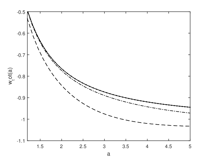
Obviously, we observe that although at late enough times we recover the de Sitter solution the total equation of state parameter can cross the phantom line (see fig. 1 ) because the scalar curvature diverges to the future, with .
III.2 Potential B
For a potential of the form
| (34) |
where
| (35) |
the Killing tensor which generates quadratic in the momentum conservation law is
| (36) |
and the boundary term is
| (37) |
where the constants , and are and .
The normal coordinates are defined by the relations
| (38) |
| (39) |
and the Lagrangian becomes
| (40) |
Hence, we find that the field equations are
| (41) |
where and and .
From (41) we have that
| (42) |
while the parameter satisfies the linear equation
| (43) |
a solution of which is
| (44) |
Notice, that equation (7) provides an additional algebraic relation for the integration constants.
For and large values of , we have that and consequently from (44) it follows that behaves like
| (45) |
where and . Hence either for large values of , the will be exponential as also from (38) the scale factor which means that the de Sitter universe is approached.
In the special case of , the normal coordinates are given by the transformation
| (46) |
Therefore, the Lagrangian of the field equations takes the simple form
| (47) |
In this context the Euler-Lagrange equations are
| (48) |
from which we find and
| (49) |
III.3 Potentials C and D
Furthermore, a quadratic in the momentum conservation law generated by the Killing tensors exists for the field equations when the potential is
| (50) |
with
| (51) |
and
| (52) |
where are the two gradient isometries of the minisuperspace (11), and is the non-gradient isometry.
The normal coordinates are given by the transformation (38), (39). In the normal coordinates the effective potential is . Using the Hamilton-Jacobi equation and the second conservation law, the field equations can be reduced to a system of nonlinear autonomous first-order differential equations. The dynamical system is one of the Lie integrable systems which have been classified in [70]. The results can be compared with the power-law solutions found in ref. [63].
The analysis that we have presented here holds for . In the limit , we can see that only the potential A provides integrability for the -gravity [34]. We continue our analysis with the study of the evolution of the field equations for the integrable potentials.
IV Dynamical evolution
We continue with the study of the critical points of the gravitational field equations. We will perform that analysis for a general potential, , so that we can determine the fixed points for the integrable potentials found in the previous sections.
First, we introduce the dimensionless variables (for instance see [71, 72, 73, 74])
| (53) |
and the new lapse function .
In the vacuum scenario, using the new variables, the gravitational field equations (7)-(9) become
| (54) |
and
| (55) |
| (56) |
| (57) |
where
| (58) |
The dynamical system (54)-(57) is a system of first-order differential equations. Also, from (54) we find the constraint
| (59) |
| (62) |
However, from (58), we see that for , , and so (61) is identically constant and only equation (60) survives.
Moreover, it is important to mention that all the cosmological parameters can be expressed in terms of the new variables. As an example, the deceleration parameter is given by
| (63) |
V Power-law potential
We continue our analysis by considering that the potential is power-law. We study separate the case in which the potential is quadratic.
V.0.1 Quadratic potential
As we have already shown above for , we have , which implies that equation (60) is simplified to
| (64) |
where the corresponding critical points are
| (65) |
At the point we find that the deceleration parameter is , which means that , hence the Brans-Dicke field is acting like a cosmological constant. On the other hand points are real when , and the deceleration parameter then takes the following forms:
| (66) |
| (67) |
One can easily check that describes an accelerating universe, since , for
As far as the stability of these points is concerned, this can be checked easily by studying the derivative of the right-hand part, of (64). Thus, we find
| (68) |
| (69) |
| (70) |
Therefore, point is always a stable attractor, while point is stable when and point is always unstable.
From the potentials of the previous section, and for we see that potential B, eqn. (34), becomes a quadratic potential for and , which means that it admits two accelerated stable points: and . For the potentials C and D, we see that only potential C can describe a quadratic potential for and , and for and . This implies that in both cases two stable points exist and they each describe an accelerating universe.
V.0.2 Potential
For a general power-law potential , with , we find that and . Hence, for the differential equation (60) we find the critical points and of (65). We would like to stress here that although the points between (60) and (65) are the same the corresponding physical parameters, such that the deceleration parameter and the stability of the critical points are different because they depend on the value of the power .
As far as the deceleration parameters are concerned we find that
| (71) |
and
| (72) |
Hence is an accelerated point as long as
| (73) |
while points provide an accelerated universe when
| (74) |
It is easy to see that describes a de Sitter point () only when that is, the quadratic potential. On the other hand, points can describe de Sitter phases for . Concerning the stability of the aforementioned points the situation is the following: is always stable as long as
| (75) |
while are stable when
| (76) |
V.1 General potential
Consider now a general potential, , which means that we have a general function . If we assume that is a solution of the algebraic equation , then we find that the system (60)-(61) admits the following critical points
| (77) |
| (78) |
and
| (79) |
From the latter, we observe that for , reduces to . On the other hand, when , point does not exist and only points exist.
The linearization of the system (60)-(61) around the point provides the following eigenvalues
| (80) |
When , or , the eigenvalues have negative real part so describes a stable spiral. On the other hand, if the condition is satisfied, then
| (81) |
and is stable. Lastly, point describes a de Sitter point, because
Concerning the eigenvalues of point we have
| (82) |
If then we find that is stable when
| (83) |
or
| (84) |
or
| (85) |
Alternatively, for , is stable when
| (86) |
or
| (87) |
or
| (88) |
V.2 Specific potentials
Consider now the potential
| (91) |
From eq.(58) we find , where , with solutions , and . Therefore, in this case there are six critical points. Points , for , and the four points , .
The point is always stable for , and the deceleration parameter is , which gives that , when . Therefore, in the special case of , we have that . Among the points only the and can be stable for , and respectively. The other two points are unstable, while the deceleration parameters are given by eqns. (66), (67).
Despite the fact that eq.(91) is a simple generalization of the quadratic potential, we can see that new critical points appear in this dynamical system. Furthermore, for the special value , is stable and it describes a de Sitter universe. This is the value at which the potential B, eqn. (34), takes the form of (91). Hence, as in the case of a minimally coupled scalar field [29], symmetries provide us with models which can describe the de Sitter phase of the universe.
For a second application we consider the potential
| (92) |
from where we calculate that with solutions Therefore, we find seven critical points, and .
Point is stable for , and it describes a de Sitter universe. Point is stable for while the stability of holds for . At , the deceleration parameters is as above, while , which shows that , when . Therefore, when the points are stable they provide an accelerated cosmological expansion. Moreover, is stable when while the rest of the points are always unstable. It is interesting to mention here that potential A with and potential B with , reduce to potential (92).
In fig. 2 we present the qualitative evolution of function for the potentials A and B in the case that the two constants are equal and for positive values of the scalar field . We observe that for positive Brans-Dicke parameters there are at least two solutions for the algebraic equation


VI Conclusions
The method of group invariant transformations and specifically the existence of contact symmetries for the field equations in the Brans-Dicke cosmology is the main focus of this work. We determined the unknown functional form of the Brans-Dicke self-interaction potential by assuming that a quadratic conservation law exists. In the case of a FLRW geometry the existence of a second conservation law leads to integrable field equations, and thus, the cosmological solution can be found by quadratures.
We determined four families of power-law potentials in which the powers depend on the value of the Brans-Dicke parameter. From these potentials only one survives for , and recover a specific theory of -gravity. Furthermore, we studied the critical points of the field equations in the vacuum scenario, using the dimensionless variables. In these variables the field equations reduce to a system of algebraic-differential equations of first order. Utilizing the algebraic equations, the final system contains two first-order ordinary differential equations, while in the limit of quadratic potential the system reduces to one first-order differential equation.
For the quadratic form of the potential we found three critical points, of which one always describes the de Sitter universe and it is stable for . For the general potential , we find that the maximum number of critical points is where is the number of solutions of the algebraic equation .
Finally, in order to demonstrate our results we considered two special forms of the potential and studied the stability of the critical points and the physical parameters. Two of the power-law families that we calculated from the application of the Killing tensors reduce to those special potentials and we derived the corresponding stable points which lead to an accelerated expansion of the universe. This is an interesting result because it coincides with previous results from other gravitational theories [75].
Acknowledgements.
JDB is supported by the STFC of the United Kingdom. AG acknowledges financial support of FONDECYT grant no. 1150246. AP acknowledges financial support of FONDECYT grant no. 3160121.References
- [1] M. Tegmark et al., Astrophys. J. 606, 702 (2004)
- [2] M. Kowalski et al., Astrophys. J. 686, 749 (2008)
- [3] E. Komatsu et al., Astrophys. J. Suppl. Ser. 180, 330 (2009)
- [4] N. Suzuki et. al., Astrophys. J. 746, 85 (2012)
- [5] Planck Collaboration: P.A.R. Ade et al., A&A 594, A13 (2016)
- [6] H.A. Buchdahl, Mon. Not. R. astron. Soc. 150, 1 (1970)
- [7] G.R. Bengochea and R. Ferraro, Phys. Rev. D 79, 124019 (2009)
- [8] V. Faraoni, Int. J. Mod. Phys. D 11, 471 (2002).
- [9] A.A. Starobinsky, Phys. Lett. B 91, 99 (1980).
- [10] R. Ferraro and F. Fiorini, Phys. Rev. D 75, 084031 (2007)
- [11] J.A.S. Lima, S. Basilakos and J. Sola, Mon. Not. R. astron. Soc. 431, 923 (2013).
- [12] B. Ratra and P.J.E. Peebles, Phys. Rev D. 37, 3406 (1988)
- [13] J.M. Overduin and F.I. Cooperstock, Phys. Rev. D 58, 043506 (1998)
- [14] S. Basilakos, M. Plionis and S. Solà, Phys. Rev. D 80 3511 (2009)
- [15] J.A.S. Lima, F.E. Silva and R.C. Santos, Class. Quantum Grav. 25 205006 (2008)
- [16] A.Y. Kamenshchik, U. Moschella and V. Pasquier, Phys. Lett. B 511, 265 (2001)
- [17] S. Pan, J. de Haro, A. Paliathanasis and R.J. Slagter, Mon. Not. R. astron. Soc. 460, 1445 (2016)
- [18] A. Paliathanasis, S. Pan and S. Pramanik, Class. Quant. Grav. 32, 245006 (2015)
- [19] R.C. Nunes and S. Pan, Mon. Not. R. astron. Soc. 459, 673 (2016)
- [20] R. de Ritis, G. Marmo, G. Platania, C. Rubano, P. Scudellaro and C. Stornaiolo, Phys. Rev. D. 42, 1091 (1990)
- [21] Y. Kucukakca, U. Camci and I. Semiz, Gen. Relativ. Gravit. 44, 1893 (2012)
- [22] S. Capozziello, S. Nesseris and L. Perivolaropoulos, JCAP 0712, 009 (2007)
- [23] Y. Kucukakca, Eur.Phys.J. C 74, 3086 (2014)
- [24] B. Vakili and F. Khazaie, Class. Quantum Gravit. 29, 035015 (2012)
- [25] B. Vakili, Phys. Lett. B 664, 16 (2008)
- [26] A. Paliathanasis, M. Tsamparlis, S. Basilakos and S. Capozziello, Phys. Rev. D 86, 063532 (2014)
- [27] R.C. de Souza, R. Adre and G.M. Kremer, Phys. Rev. D 87, 083510 (2013)
- [28] P.A. Terzis, N. Dimakis and T. Christodoulakis, Phys. Rev. D 90, 123543 (2014)
- [29] A. Paliathanasis, M. Tsamparlis, S. Basilakos and J.D. Barrow, Phys. Rev. D 93, 043528 (2016)
- [30] J. A. Belinchón, T. Harko and M.K. Mak, Astrophys Space Sci. 361, 52 (2016)
- [31] H. Wei, X.J Guo and L.F. Wang, Phys. Lett. B 707, 298 (2012)
- [32] B. Modak, S. Kamilya and S. Biswas, Gen. Relativ. Gravit. 32, 1615 (2000)
- [33] A. Paliathanasis, M. Tsamparlis and S. Basilakos, Phys. Rev. D 90, 103524 (2014)
- [34] A. Paliathanasis, Class. Quantum Gravit. 33, 075012 (2016)
- [35] P. Fré, A. Sagnotti and A.S. Sorin, Nucl. Phys. B 877, 1028 (2013)
- [36] V.V. Sokolov and A.S. Sorin, Integrable Cosmological Potentials, [arXiv:1608.08511]
- [37] A.Yu. Kamenshchik, E.O. Pozdeeva, A. Tronconi, G. Venturi and S.Yu. Vernov, Class. Quantum Grav. 31, 105003 (2014)
- [38] A. Paliathanasis, J.D Barrow and P.G.L. Leach, Phys. Rev. D 94, 023525 (2016)
- [39] N. Dimakis, A. Karagiorgos, A. Zampeli, A. Paliathanasis, T. Christodoulakis and P.A. Terzis, Phys. Rev. D 93, 123518 (2016)
- [40] A. Zampeli, T. Pailas, P.A. Terzis and T. Christodoulakis, JCAP 05, 066 (2016)
- [41] H. Suzuki, E. Takasugi and Y. Takayama, Mod. Phys. Lett. 11, 1281 (1996)
- [42] P. Parsons and J.D. Barrow, Class. Quantum Gravit. 12, 1715 (1995)
- [43] J.D. Barrow and P. Parsons, Phys. Rev. D 52, 5576 (1995)
- [44] J.D. Barrow, Phys. Rev. D 48, 1585 (1993)
- [45] E.O. Kahya, B. Pourhassan and S. Uraz, Phys. Rev. D 92, 103511 (2015)
- [46] A.A. Coley, J. Ibáñez and I. Olasagasti, Phys. Lett. A 250, 75 (1998)
- [47] A. Billyard, A. Coley and J. Ibáñez, Phys. Rev. D 59, 023507 (1998)
- [48] P. Jordan, Nature 164, 637 (1937) and Schwerkraft und Weltfall, 2nd ed. (Vieweg und Sohn, Braunschweig, 1955)
- [49] C.H. Brans and R.H Dicke, Phys. Rev. 124, 925 (1965); L.E. Gurevich, A.M. Finkelstein and V.A. Ruban, Astrophys. Space Sci. 22, 231 (1973); D. J. Holden, D. Wands, Class.Quant.Grav., 15, 3271 (1998); J.D. Barrow, Mon. Not. R. Astr. Soc., 282, 1397 (1996)
- [50] S. Sen and A.A. Sen, Phys. Rev. D 63, 124006 (2001)
- [51] B. Boisseau, G. G. Esposito-Farese, D. Polarski and A. A. Starobisky, Phys. Lett., 85 2236 (2000); G. Esposito-Farese and D. Polarski, Phys. Rev. D. 63 063504 (2001); D.E Torres, Phys. Rev. D. 66 043522 (2002); T. Clifton, J.D. Barrow and R. Scherrer, Phys. Rev. D 71, 123526 (2005)
- [52] T. Clifton, P. G. Ferreira, A. Padilla and C. Skordis, Phys. Rep., 513, 1 (2012)
- [53] L. Amendola and S. Tsujikawa, Dark Energy Theory and Observations, Cambridge University Press, Cambridge UK, (2010)
- [54] V. Faraoni, Phys. Rev. D59, 084021, (1999)
- [55] B. Bertotti, L. Iess and P. Tortora, Nature 425, 374 (2003)
- [56] A. Scharer, R. Angelil, R. Bondarescu, P. Jetzer,A. Lundgren, Phys. Rev. D., 90, 123005 (2014)
- [57] A. R. Liddle, A. Mazumdar and J. D. Barrow, Phys. Rev. D 58, 027302 (1998)
- [58] X. Chen and M. Kamionkowski, Phys. Rev. D 60, 104036 (1999).
- [59] T.P. Sotiriou and V. Faraoni Rev. Mod. Phys. 82, 451 (2010).
- [60] C.G. Callan, D. Friedan, E.J. Martinez, and M.J. Perry, Nucl. Phys. B 262, 593 (1985); E.S. Fradkin and A.A. Tseytlin, Nucl. Phys. B 261, 1 (1985).
- [61] Y. M. Cho, Phys. Rev. Lett 68, 3133 (1992)
- [62] V. Faraoni, Cosmology in Scalar-Tensor Gravity, Fundamental Theories of Physics vol. 139, (Kluwer Academic Press: Netherlands, 2004)
- [63] J.D. Barrow and K-i Maeda, Nucl. Phys. B 341, 294 (1990)
- [64] C.H. Brans and R.H. Dicke, Phys. Rev. 124, 925 (1961)
- [65] J. O’Hanlon, Phys. Rev. Lett. 29, 137 (1972)
- [66] W. Sarlet and F. Cantrijn, SIAM Review 23, 467 (1981)
- [67] T.M. Kalotas and B.G. Wybourne, J. Phys. A 15 2077 (1982)
- [68] P.A. Terzis, N. Dimakis, T. Christodoulakis, A. Paliathanasis and M. Tsamparlis, J. Geom. Phys. 101, 52 (2016)
- [69] M. Tsamparlis and A. Paliathanasis, J. Phys. A: Math. Theor. 45, 275201 (2012)
- [70] C. Daskaloyannis and K. Ypsilantis, J. Math. Phys. 47, 042904 (2006)
- [71] O. Hrycyna and M. Szydlowski, JCAP 12, 016 (2013)
- [72] R. Garcia-Salcedo, T. Gonzalez and I. Quiros, Phys. Rev. D 92, 124056 (2015)
- [73] A. Cid, G. Leon and Y. Leyva, JCAP 16, 027 (2016)
- [74] G. Leon, Class. Quant. Grav. 26, 035008 (2009)
- [75] J.D. Barrow and D.J. Shaw, Class Quantum Gravity 25, 085012 (2008)