Seafloor identification in sonar imagery via simulations of Helmholtz equations and discrete optimization

As in the majority of fluid-sediment modeling [13, 23, 24], we treat the sediment layer as a fluid and model time-harmonic acoustic pressure waves as solutions $p$ to Helmholtz equations with varying coefficients,

where $\omega$ is the frequency variable. The model coefficients represent the sound speed $c$ and material density $\rho$, given in the water layer by $c_{0}=1030$ m/s² and $\rho_{0}=1500$kg/m³. The attenuation of high frequency acoustic waves in the sediment is given by $\gamma$, and we assume that the attenuation in water is negligible.

There are two coupling conditions on the interface in (3). The first is a continuity of pressure along the fluid-sediment interface. The second condition is the continuity of displacement normal to the boundary of the interface. Here the vector $\vec{n}$ is normal to the curve given by $(x,f(x))$ and $|_{+}$ and $|_{-}$ refer to the limits of a function or derivative as $y$ approaches $y=f(x)$ from above and below, respectively. As a remark, in situations where it is desirable to model more that one sedimentary layer, this model can be augmented with additional interface conditions of the type (3) and equations of the type (4).

For boundary conditions, the fast attenuation in the sediment layer is modeled with the condition $p=0$ on the lower boundary of the domain, and absorbing boundary conditions representing the incoming wave are imposed on the upper boundary. In general, the conditions on the left and right boundaries are determined by the assumptions on scattering contributions from neighboring sediment layers.

The process begins when an acoustic pulse, called a ping, is generated by a source near the surface. Close to the seafloor, the signal acts as an incident plane wave traveling in the direction given by the vector $k_{\alpha}=(k\cos\alpha,-k\sin\alpha)$, where $\alpha$ is the incident angle and $k=\frac{\omega}{c}$ is the wavenumber (see Figure 3). Supposing that the strength of the source is $P_{0}$, the incident wave $p_{inc}$ in the domain $D$ is expressed as

The interaction of these waves with the seafloor produces outgoing waves in multiple directions depending on the roughness and material type of the sediment layer. Sufficiently far from caustics, the scattered wavefield $p_{out}$ can be approximated by the superposition given by

where $P_{\beta}(x,y)$ is the complex amplitude of the outgoing wave in the direction $\beta$.

The typical spatial domain $\Omega$ is large, on the order of kilometers, while the acoustic wavelength is a few centimeters. A domain of size 100 m covers thousands of times the acoustic wavelength of a 20 kHz source signal in range, and tens of wavelengths in depth [17]. Full resolution of the signal in the water layer alone would require a grid of at least five points per wavelength, on the order of hundreds of millions of points for 2D resolution. Several predictions of the forward model must be made in the template matching process, and the computational task quickly becomes too expensive.

The original model can be reduced by dividing the domain $D$ into $N$ disjoint segments of length $\Delta s$, and determining the backscattering caused by the seafloor occupying the $i^{th}$ segment of the seafloor domain,

The width $\Delta s$ of each segment is chosen to be roughly $10-20$ times the acoustic wavelength. Then, we can reasonably assume that the scattering features of interest in each segment of length $\Delta s$ is independent from segments that are spatially far away and approximate the backscattering using only local simulations. We will then design a procedure for approximating the backscattering (7) on small domains, each of size $\Delta s$ using a 1) parametrization of the seafloor and 2) localized simulations.

A simplified description of the seafloor domain can be made by assigning a vector of parameters $m^{i}$ that describe the seafloor properties within segment $D^{i}$. The identification of seafloor parameters that can be recovered from backscattered data can enable efficient predictions of the scattering effects from a wide range of sea floors. Seafloor parameters fall into three main categories: experimental parameters, geometric parameters, and geoacoustic parameters. Experimental parameters $m_{E}$ are determined from the physical scenario, and it will be assumed that these parameters are known beforehand. Within the segment $D^{i}$ it can be assumed, for our purposes, that the geometric parameters $m_{G}$ can be modeled as smoothly varying functions that take a continuous range of values. Though the full seafloor domain consists of many sediment types, we assume that each seafloor patch, when it is small enough, consists of a uniform sediment, that is, $m_{A}$ remains constant. The parameter $m_{A}$ is qualitative; we will assign to the segment $D^{i}$ one label from a list of possible material types. Descriptions of the categories are below:

• 1.

  Experimental parameters, $m_{E}$. These parameters include the locations of the source and receiver, source strength, source frequency, and incident angle. The source and receiver locations are colocated near the surface of the water, and the strength of the acoustic source is a constant and given by the sonar manufacturer. For sidescan sonars this is typically between $200-230$ decibels [35]. High frequency signals produce strong scattering from artifacts in the seabed that have variations on the scale of the acoustic wavelength. These artifacts cannot be easily detected using lower frequencies. We consider source signal s with a frequency of 20 kHz. The acoustic wavelength is then on the scale of centimeters. The range of the incident angle $\alpha$ is determined by the instrument. Specifically, in sidescan sonars, $\alpha$ lies within the critical range of $30^{\circ}\pm 15^{\circ}$.

• 2.

  Geometric parameters, $m_{G}$. The interface function $f(x)$ depends on fine scale features, such as the surface roughness characteristic, and large scale features, such as the overall curvature of the interface. Statistical models of seafloor roughness parameterize the distribution of the normalized amplitude of representative component sinusoids [17]. The idea is to mimic a realistic seabed that is not necessarily periodic. The parametrization of $f$ can be more general, but in this study, we model a seabed with sinusoidal ripples as an example,

  $\displaystyle m_{G}\rightarrow f(x,m_{G})=.01\left(\sin(2\pi m_{G1}x)+m_{G2}\sin(2\pi m_{G3}x)\right).$

  (9)

  The geometric parameter $m_{G}=(m_{G1},m_{G2},m_{G3})$ refers to the frequencies $m_{G1}$ and $m_{G3}$ and aspect ratio $m_{G2}$ of the component sinusoids. The choice of spatial frequencies $m_{G1}\simeq 15$ and $m_{G3}\simeq 25$ produces a spatial variations on a scale similar to the characteristic wavelength of the incoming acoustic wave (see Figure 3). We chose values for the aspect ratio that lie in the interval $.5\leq m_{G2}\leq 1$.

• 3.

  Geoacoustic parameters, $m_{A}$. The acoustic description of the the sound speed, density, and attenuation, is purely based on material type of the sediment layer. The influence of the material type is not explicitly used in the interface function, however it is in practice reflected in the fine scale ranges of the acoustic response. For example, the fine scales for mud, sand, sea grass, and rock are of an increasing order in their characteristic length scales.

  Here, we included sediment types with distinctive geoacoustics. The sound speed in fine sediments such as clay are typically “slow” (1-5% less than water), while the speed in sand is “fast” (10-15% more than water) [23]. In all of these sediments, the sound attenuation $\gamma$ is roughly 0.5 dB per 1 meter per 1 kHz. We chose not to distinguish attenuation based on material type. In Table 1, the density $\rho_{m_{A}}$ and sound speed $c_{m_{A}}$ of the different materials used in this study is given.

  Material type	density (kg/m3)	sound speed (m/s)
  sand	$\rho_{sand}=2000$	$c_{sand}=1668$
  clay	$\rho_{clay}=1170$	$c_{clay}=1518.9$
  rock	$\rho_{rock}=2870$	$c_{rock}=6000$
  metal	$\rho_{metal}=8050$	$c_{metal}=6100$

  The possible material types $m_{A}$ that represent the sediment layer are

  $\displaystyle m_{A}=\text{`sand', `clay', `rock', or `metal'}.$

  A typical sediment layer is depicted in Figure 4 (a). The material type $m_{A}=$ ‘metal’ is used to label a sand layer containing a buried rectangular metal object, however this can easily be extended to objects buried in other sediments or objects that are only partially buried. The metal domain, depicted in Figure 4 (b), is $D^{\prime}\cap\{y<-\epsilon_{f}\}$. The object lies purely beneath the interface, $\text{inf}_{x}f(x)+\epsilon_{f}>0$. The depth parameter $\epsilon_{f}>0$ is chosen to be large enough so that the object can be detected using high frequency waves. If $\epsilon_{f}$ is too large, other techniques must be used, for example, using lower frequency pings. In this study we only considered objects buried in a sediment layer of sand, however this can easily be extended to objects buried in other sediments or objects that are only partially buried.

  In summary, the sediment layer $D^{\prime}\cap\{y<f\}$ is assigned the geoacoustic properties $m_{A}\rightarrow(\rho_{m_{A}},c_{m_{A}})$ for $m_{A}=\text{sand, clay, rock,}$. For $m_{A}=\text{metal}$, these properties are given by

  $\displaystyle m_{A}\rightarrow\begin{cases}(\rho_{sand},c_{sand})&-\epsilon_{f}<y,\\ (\rho_{metal},c_{metal})&y<-\epsilon_{f}\end{cases}.$

  (10)

We chose a parameter space $\mathcal{M}$, consisting of acoustic and geometric parameters,

where $m_{A}$ is a parameter that determines the sound speed and density of the sediment and $m_{G}$ determines the interface function.

For large seafloor domains, simulations of high frequency Helmholtz equations are often cost-prohibitive. A key component of our framework involves determining the acoustic response of smaller spatial segments of seafloor domain by matching the observed acoustic response with a collection of precomputed signals. These signals, called acoustic templates, represent the backscattering from small patches of the sediment layer with the typical geometric and material characteristics. Based on the previous discussion, a vector of parameters $m=(m_{A},m_{G})$ can be used to describe each segment $D^{i}\subset D$. Forward simulations can be used to determine the contribution to the backscatter from the parameterized seafloor.

Let $D^{\prime}\subset D$ be a generic template domain of width $\Delta s$, and for $m\in\mathcal{M}$, define the interface function $f$ determined by $m_{G}$ and the formula (9). In the sediment layer $D^{\prime}\cap\{y<f\}$, the density and sound speed of the material are determined by $m_{A}$ as in (10). Then, the solution $\hat{p}_{m}$ to the Helmholtz equations $\text{(\ref{eq:fwd1})}-\text{(\ref{eq:fwd3})}$ approximates the scattering from the seabed. Let $\hat{b}_{m}$ be the backscatter computed from $\hat{p}_{m}$ in the domain $D$ given by (7). Then, the acoustic response for each segment of the seabed has the correspondence

The boundary conditions in the local model $\text{(\ref{eq:fwd1})}-\text{(\ref{eq:fwd3})}$ must be chosen carefully. As a result of our scale assumptions, the vast majority of segments $D^{i}\subset D$ have the same material type as the neighboring segments $D^{i-1}$ and $D^{i+1}$. For simplicity, we impose periodic boundary conditions that account for the scattering contributions from neighboring domains of the same material type and geometry. This is a common strategy in scattering theory in the context of micro-optics, where periodic structures are called diffraction gratings [3, 4, 5, 10].

On the other hand, there are instances where segments of the domain differ in material type from neighboring segments. For each $i=1,\ldots N-1$, we will call the pair of material types in the cells $D^{i}$ and $D^{i+1}$ a “transition” at the location $x=i\Delta s$. For example, the sediment layer shown in Figure 4 (c) contains a ‘sand-clay’ transition at location $x=i\Delta s$. Sediment layers containing a transition can be modeled by embedding the template domain into a larger domain in which periodic boundary conditions are imposed.

The sources of modeling error include the local representation of the backscatter using truncated domains, the smoothness assumptions on the parameters, and any resonance phenomena occurring from the choice of periodic boundary conditions.

Due to the fine scale structure of the seafloor, interactions between the sediment layer and the the incoming acoustic wave produce complex scattering effects. The modeling of synthetic backscatter requires accurate details about the propagation of outgoing waves, especially the waves that propagate along the receiver direction. This motivates the need for strategies for extracting information from the solution $p$ to the Helmholtz equation $\text{(\ref{eq:fwd1})}-\text{(\ref{eq:fwd3})}$ that represents the backscattered signal $Y\in{\mathbb{R}}^{n}$ given by (7).

Common approaches for modeling the scattering effects are based on geometric ray tracing or full solutions to wave equations [6, 16]. Approaches such as Kirchhoff approximation (requiring the seafloor interface to be smooth) and small perturbation theory (requiring the roughness scale to be much smaller than the acoustic wavelength) are independent of the wave theory used and do not account for volume scattering within the sediment [21, 24]. Furthermore, many models for seafloor backscatter are often developed for only seabeds consisting of isotropic roughness.

Here, we use a different tool that is sensitive to the underlying seafloor material properties as well as microtopography. Our proposed strategy has two components. The first component involves modeling scattering by interpreting solutions to Helmholtz equations as superpositions of waves traveling in different directions. The second component involves modeling the backscattered signal $Y$ and extracting information about the waves traveling in the backscattered direction.

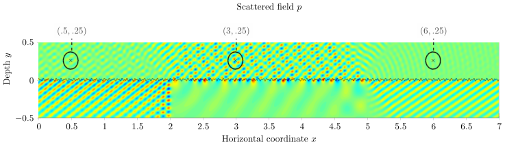
The measured scattering from the seabed is approximated using numerical microlocal analysis of solutions to Helmholtz equations, a technique for determining the number, directions, and the corresponding complex amplitudes of the crossing rays in domains where geometric optics is valid. Described in detail in [7, 30], the main idea is that if observation points $(x_{0},y_{0})$ are far away from caustics and focus points and the wavelength $\lambda_{0}=2\pi/k$ contains variations on a scale sufficiently small with respect to the geometry, the solution $p(x,y)$ to $\text{(\ref{eq:fwd1})}-\text{(\ref{eq:fwd3})}$ behaves like a superposition of plane waves. Adopting the notation in [7, 30], the local plane wave approximation of $p(x,y)$ restricted to a circle centered at $(x_{0},y_{0})$ with sufficiently small radius $r_{0}$ is

when $|(x,y)-(x_{0},y_{0})|<r_{0}$ (Figure 5). The values of $P_{\beta_{l}}(x,y)$ correspond to the complex amplitudes of the outgoing waves traveling in the directions $\phi_{l}=(\cos(\beta_{l}),\sin(\beta_{l}))$. The function $P_{\beta_{l}}(x,y)$ is locally smooth and independent of wavelength.

The algorithm recovers the number $L$ of crossing rays and the magnitudes $|P_{\beta_{l}}(x_{0},y_{0})|$ of the scattered waves in the direction given by $\beta_{l}$. In the derivation, the 2-D Jacobi-Anger expansion is used to represent the local solution as a series involving Bessel functions, which is then appropriately truncated at a threshold $\hat{L}(r_{0})=r_{0}+5r_{0}^{1/3}$. Finally, the desired $L=2\hat{L}(r_{0})+1$ unknown amplitudes are determined using a Fourier-type inversion formula involving the Bessel function of order $l$, denoted by $J_{l}(r_{0})$. Regularization can be applied to improve the stability of the reconstruction formula.

The following steps summarize the algorithm for approximating the backscattering at each observation point $(x_{0},y_{0})$:

Step 1. Define $L$ equidistant points on the interval $[0,2\pi)$,

$\displaystyle\beta_{l}=\frac{2\pi({l}-1)}{L},\qquad{l}=1,\ldots,L,$

and let $\{\tilde{P}_{l}\}$ be the grid function of sampled values of the Helmholtz solution $p(x,y)$ on the restricted circle centered at the observation point $(x_{0},y_{0})$ with radius $r_{0}/k$, $r_{0}=3\pi$ and angles $\beta_{l}$,

$\displaystyle{\tilde{P}_{l}}=p\left(x_{0}+\frac{r_{0}}{k}\cos(\beta_{l}),y_{0}+\frac{r_{0}}{k}\sin(\beta_{l})\right),\qquad{l}=1,\ldots,L.$

Step 2. Let $\epsilon>0$ be a regularization parameter, and denote by $FFT$ and $FFT^{-1}$ the discrete Fourier transform and the inverse discrete Fourier transform, respectively. Define

$\displaystyle\{p_{l}^{\epsilon}\}=2\pi FFT^{-1}\left\{\frac{FFT\{\tilde{P}_{l}(2\hat{L}(r_{0})+1)J_{l}(r_{0})\}}{i^{q}[(2\hat{L}(r_{0})+1)^{2}J_{q}(r_{0})^{2}+4\epsilon\pi^{2}]}\right\}$

Step 3. $|P_{\beta_{l}}(x_{0},y_{0})|\simeq|p_{l}^{\epsilon}|$.

Figure 6 shows the resulting polar plots of $|p_{l}^{\epsilon}|$ taken at the three observation points indicated in Figure 5. Figure 7 gives a surface plot of the scattering $|p_{l}^{\epsilon}|$ at measurements taken across the full spatial domain (horizontal axis) and full range of scattering directions $\beta$ (vertical axis).

In the sonar applications of present interest, receivers only detect the strength of signals propagating in the backscattered direction $\beta=\alpha$. We estimate this quantity using linear interpolation between values in the given pairs $(\beta_{l},p^{\epsilon}_{l})$. For $\beta$ is in the interval $[\beta_{l},\beta_{l+1})$, the amplitude of the backscattered wave (7) is approximated by

The optimization process is a greedy table-lookup method, where regularization is imposed using constraints based on the parameters chosen for neighboring templates. Another option would be to use machine learning techniques such as neural networks in the identification [20]. In each segment of the domain, the algorithm determines a match from the collection of templates in the library $\mathcal{L}$ for the truncated signal $(b_{i})_{j}=(Y)_{j}$ restricted to the $i^{th}$ segment of the measurement domain, $X\cap D^{i}$. It is assumed that the observations $b_{i}$ and templates $\hat{b}_{m}\in\mathcal{L}$ are both vectors of length $2^{N_{1}}$ for an integer $N_{1}$. The wavelet coefficients of $b_{i}$ and $\hat{b}_{m}$ are given by $(w_{i}^{l},v_{i}^{l})$ and $(\hat{w}^{l}_{m},\hat{v}^{l}_{m})$, respectively.

The data misfit functions are defined for each segment of the domain and wavelet level,

Define $\mathcal{L}^{L_{max}+1}_{i}=\mathcal{L}$. The set $\mathcal{L}^{l}_{i}\subseteq{\mathcal{L}}^{l+1}_{i}$ is a collection of candidate templates $\hat{b}_{m}$ from the library that produce a sufficiently small value of the misfit function given by (17). For a given tolerance $\epsilon>0$, these sets are given by

Since the maximum stage in the wavelet decomposition results in coefficient vectors of the smallest length, it is efficient to begin the matching process at the stage $l=L_{max}$. After the set $\mathcal{L}_{i}^{L_{max}}$ is determined, the decomposition level is decreased, $l=L^{max}-1$, and repeating the search process among the candidate templates $\hat{b}_{m}\in\mathcal{L}^{L_{max}}_{i}$, a refined set of candidate templates $\mathcal{L}^{L_{max}-1}_{i}\subseteq\mathcal{L}^{L_{max}}_{i}$ is produced. This process is iterated for each further stage, $l=L_{max}-2,\ldots,l^{*}$, until either $l^{*}=1$ or the pool of candidate templates $\mathcal{L}^{l^{*}-1}_{i}$ contains no templates.

If the set $\mathcal{L}^{l^{*}}_{i}$ contains multiple candidate templates, the choice for the seafloor parameter $m_{i}$ in the set $\mathcal{M}_{i}^{*}=\{m\in\mathcal{M}\mid\hat{b}_{m}\in\mathcal{L}^{l^{*}}_{i}\}$ is made using information about spatially neighboring segments of the domain. There is no penalty term for the selection of ${m}^{1}$ corresponding to the leftmost segment of the domain. The penalty term for $i>1$ is weighted by a fixed parameter $\delta>0$ and is given by

where $m^{\prime}_{G}$ and $n^{\prime}_{G}$ indicate the geometric parameters.

The algorithm for finding the best template match in each segment $i=1,\ldots N$, is summarized below.

1. 1.

   Preliminary candidate search using multilevel wavelet decomposition: Set $l=L_{max}$.

   1. (a)

      Candidate templates at level $l$ are given by $\mathcal{L}^{l}_{i}$.

      1. i.

         If $\mathcal{L}^{l}_{i}=\emptyset$, then $l^{*}=l+1$ and $\mathcal{L}_{i}^{{l^{*}}}$ is returned.

      2. ii.

         If $l=1$, then $l^{*}=1$ and $\mathcal{L}_{i}^{{l^{*}}}$ is returned.

   2. (b)

      The wavelet level is decreased, $l=l-1$.

2. 2.

   The final parameter choice depends on the chosen parameters in the preceding segment of the domain,

   $\displaystyle{m}^{i}=\underset{m^{\prime}\in\mathcal{M}^{*}_{i}}{\text{argmin}}\{G_{i}^{{l^{*}}}(\hat{b}_{m^{\prime}})+\delta R_{i}(m^{\prime},m^{i-1})\}.$

3. 3.

   The estimated seafloor parameters are ${\bf m}=(m^{1},\ldots,m^{N})$ and the strength of the backscattered signal on the large domain is approximated by

   $\displaystyle\hat{Y}=F[{\bf{m}}].$

For a well-chosen tolerance level, the number of candidate templates will be significantly reduced in each iteration, resulting in the nested sets,

The computational gain comes from this design; as the level of detail required to compare the signals is increased, the number of possible candidate templates decreases. The misfit function (17) is evaluated for all templates in the library only in the first iteration $l=L_{max}$, when the number of the wavelet coefficients in the vectors $\hat{w}^{l}_{m}$ and $\hat{v}^{l}_{m}$ is the smallest. As $l$ decreases, the number of wavelet coefficients in the vectors $\hat{w}^{l}_{m}$ and $\hat{v}^{l}_{m}$ increases, however the number of evaluations of the misfit (17) is lowered due to a reduced search space $\mathcal{L}^{l}_{i}\subset\mathcal{L}^{l+1}_{i}$.

We examined the effects of enriching the library using templates with multiple materials in terms of the rate of false detections of objects. In this experiment, we executed the classification algorithm on 100 different realizations of the data polluted with 5% noise. To demonstrate the need for an enriched library, the algorithm was performed first on the library $\mathcal{L}_{0}$ containing templates with material parameters $m_{A}=$ ‘clay’, ‘sand’, ‘rock’, and ‘metal’. In Table 3 the left column is a list of the transition types at locations $x=i\Delta s$ corresponding to the segments $D^{i}$ that were incorrectly identified by our method as ‘metal’. The second and third columns show the false alarm rate corresponding to Model A and Model B, respectively. The false alarm rate is defined as ratio of the number of times the segment was labeled as a ‘metal’ and the number of instances of that transition in the 100 trials. For example, there are instances of ‘sand-sand’ in the material parameter (19) at the four locations $x=1,2,3,4$. Out of 100 trials, there were three false detections at one of these locations, therefore the false alarm rate is $3/(100\times 4)$.

Then, the algorithm was performed on an enriched library $\mathcal{L}$ containing additional signals generated using synthetic seabeds containing a transition between two different materials, i.e., ‘sand-clay’, ‘clay-sand’, ‘clay-rock’, ‘sand-metal’. The ‘sand’ and ‘clay’ templates generated from a seabed of length $2\Delta s$ containing the ‘sand-clay’ and ‘clay-sand’ transitions. Templates with material types ‘sand’, ‘clay’, and ‘metal’ were added using seabeds containing the ‘clay-rock’ and ‘sand-metal’ type. Table 3 indicates the main cause of false alarms is the presence of the ‘clay-rock’ transition in the synthetic seabed. Segments of the domain that were a part of other transition types also contribute to the false alarm rate, however, the contribution is minimal in comparison.

Many well-studied approaches for determining the resolution needed to classify objects rely on ideas from information theory, for example, finding the resolution needed to to distinguish a sphere from a cube [29, 34, 36]. The proposed methods give a way to approach this problem using simulations of seabeds containing buried objects of varying size. Table 3 shows the detection rate, defined as is the number of times a segment $D^{i}$ containing a submerged object was correctly identified divided by the number of trials.

From these results, we conclude that the template domain size influences the recovery. For example, the smallest object with a width of .5 meters is rarely detected in Model A and not well-detected in Model B. In Model A, the objects can be detected by our algorithm to a resolution of $\Delta s=1$m with high accuracy. The higher detection rate for 2 meter objects over 4 meter objects in Model B might be explained by the location of the object near the boundary of the computational domain. In both cases, we believe that reducing the size of the template domain will increase the resolution of object detection. Also, we expect that enriching the library of templates to include more geometry parameters will improve the detection rate in Model B. Figure 10 contains plots of the noisy signals (20) and reconstructions using the proposed method. Though the geoacoustic properties of rock and metal are similar, the method correctly differentiated between the two.

Though the primary aim of the proposed method is to properly identify objects based on material type, we also looked at how well the geometric parameters $m_{G}$ were recovered. In Model A, the geometric parameters are fixed and in Model B these parameters vary linearly across the domain. Figure 11 shows the distribution of relative errors in the reconstructed parameters $m_{G1}$, $m_{G2}$ and $m_{G3}$. The relative error formulas for the geometric parameters are

In the library, there were two possibilities for the second geometric parameter, $m_{G2}=.5$ and $m_{G2}=1$. Since the seafloor model parameters (18) are constant, the error distribution of $E_{2}$ is split into correct estimates and incorrect estimates. The error distribution for Model B reflects the smooth changes in across the measurement domain.

References

- [1] COMSOL AB. COMSOL Multiphysics® v. 5.2. www.comsol.com.
- [2] Arthur B Baggeroer, W A Kuperman, and Henrik Schmidt. Matched field processing: Source localization in correlated noise as an optimum parameter estimation problem. Journal of Acoustic Society of America, 83(2):571–587, 1988.
- [3] Gang Bao. Finite element approximation of time harmonic waves in periodic structures. SIAM Journal on Numerical Analysis, 32(4):1155–1169, 1995.
- [4] Gang Bao and Peijun Li. Inverse medium scattering for the Helmholtz equation at fixed frequency. Inverse Problems, 21:1621–1641, 2005.
- [5] Gang Bao and Peijun Li. Near-field imaging of infinite rough surfaces. SIAM Journal on Applied Mathematics, 73(6):2162–2187, 2013.
- [6] Judith M. Bell. Application of optical ray tracing techniques to the simulation of sonar images. Optical Engineering, 36(6):1806–1813, 1997.
- [7] Jean David Benamou, Francis Collino, and Olof Runborg. Numerical microlocal analysis of harmonic wavefields. Journal of Computational Physics, 199(2):717–741, 2004.
- [8] T. Beokett and Donald Hussong. Digital image processing techniques for enha , cement and classification of SeaMARC II side scan sonar imagery. Journal of Geophysical Research, 94(B6):7469–7490, 1989.
- [9] Philippe Blondel. The Handbook of Sidescan Sonar. Springer Berlin Heidelberg, Berlin, Heidelberg, 2010.
- [10] Oscar Bruno and Fernando Reitich. Solution of a boundary value problem for Helmholtz equation via variation of the boundary into the complex domain. 1991.
- [11] David S Burnett. Computer simulation for predicting acoustic scattering from objects at the bottom of the ocean. Acoustics Today, 11(1):28–36, 2015.
- [12] Pierre Cervenka and Christian De Moustier. Sidescan Sonar Image Processing Techniques. IEEE Journal of Oceanic Engineering, 18(2):108–122, apr 1993.
- [13] David M. F. Chapman. What Are We Inverting For? In Inverse Problems in Underwater Acoustics, pages 1–14. Springer New York, New York, NY, 2001.
- [14] J Del Rio Vera, E Coiras, J Groen, and B Evans. Automatic Target Recognition in Synthetic Aperture Sonar Images Based on Geometrical Feature Extraction. EURASIP Journal on Advances in Signal Processing, 2009:1–10, 2009.
- [15] Gerald J Dobeck. Algorithm Fusion for Automated Sea Mine Detection and Classification. In MTS/IEEE Oceans 2001. An Ocean Odyssey. Conference Proceedings (IEEE Cat. No.01CH37295), pages 130–134, 2001.
- [16] Gareth R. Elston and Judith M. Bell. Pseudospectral time-domain modeling of non-Rayleigh reverberation: Synthesis and statistical analysis of a sidescan sonar image of sand ripples. IEEE Journal of Oceanic Engineering, 29(2):317–329, apr 2004.
- [17] Christopher G. Fox and Dennis E. Hayes. Quantitative methods for analyzing the roughness of the seafloor. Reviews of Geophysics, 23(1):1, 1985.
- [18] George V. Frisk. Environmental influences on low-frequency, shallow-water acoustic propagation and inversion. The Journal of the Acoustical Society of America, 125(4):2590–2590, apr 2009.
- [19] Andrew Glassner, editor. An Introduction to Ray Tracing, volume 8. Morgan Kaufmann Publishers, San Francisco, 1989.
- [20] R. Paul Gorman and Terrence J. Sejnowski. Analysis of hidden units in a layered network trained to classify sonar targets. Neural Networks, 1(1):75–89, 1988.
- [21] J. Groen, E. Coiras, J. Del Rio Vera, and B. Evans. Model-based sea mine classification with synthetic aperture sonar. IET Radar, Sonar & Navigation, 4(1):62, 2010.
- [22] Pat Hanrahan and Wolfgang Krueger. Reflection from layered surfaces due to subsurface scattering. Proceedings of the 20th annual conference on Computer graphics and interactive techniques, pages 165–174, 1993.
- [23] Darrell R. Jackson and Michael D. Richardson. High-Frequency Seafloor Acoustics. Springer, New York, New York, USA, 2007.
- [24] Darrell R. Jackson, D.P. Winebrenner, and A. Ishimaru. Application of the composite roughness model to high-frequency bottom backscattering. The Journal of the Acoustical Society of America, 79(May):1410, 1986.
- [25] Finn B. Jensen, William A. Kuperman, Michael B. Porter, and Henrik Schmidt. Chapter 2 Wave Propagation Theory. In Computational Ocean Acoustics, pages 65–154. Springer New York, New York, NY, 2011.
- [26] Henrik Wann Jensen, Stephen R. Marschner, Marc Levoy, and Pat Hanrahan. A practical model for subsurface light transport. Siggraph, pages 511–518, 2001.
- [27] Steven G. Kargl, Aubrey L. Espana, Kevin L. Williams, Jermaine L. Kennedy, and Joseph L. Lopes. Scattering From Objects at a Water???Sediment Interface: Experiment, High-Speed and High-Fidelity Models, and Physical Insight. IEEE Journal of Oceanic Engineering, 40(3):632–642, 2014.
- [28] Steven G. Kargl, Kevin L. Williams, and Aubrey L. Espana. Fast model for target scattering in a homogeneous waveguide. The Journal of the Acoustical Society of America, 132(3):1909, 2012.
- [29] Ronald T. Kessel. Estimating the limitations that image resolution and contrast place on target recognition. Automatic Target Recognition XII. Proceedings of SPIE, 4726:316–327, jul 2002.
- [30] Yanina Landa, Nicolay M. Tanushev, and Richard Tsai. Discovery of point sources in the Helmholtz equation posed in unknown domains with obstacles. Communications in Mathematical Sciences, 9(3):903–928, 2011.
- [31] X. Lurton. An Introduction to Underwater Acoustics Principles and Applications. Springer, 2010.
- [32] Stephane G. Mallat. A Theory for Multiresolution Signal Decomposition: The Wavelet Representation. IEEE Transactions on Pattern Analysis and Machine Intelligence, 11(7):674–693, jul 1989.
- [33] Patrick S. McCormick, Ji Qiang, and Robert D. Ryne. Visualizing underwater environments using multi-frequency sonar. IEEE Computer Graphics and Applications, 19(5):61–65, 1999.
- [34] V. Myers and M. Pinto. Bounding the performance of sidescan sonar automatic target recognition algorithms using information theory. IET Radar, Sonar & Navigation, 1(4):266–273, 2007.
- [35] Yan Pailhas, Yvan Petillot, and Chris Capus. High-resolution sonars: What resolution do we need for target recognition?, 2010.
- [36] M. Pinto. Performance index for shadow classification in minehunting sonar - Google Scholar. In Proceedings of the UDT Conference, 1997.
- [37] James C. Preisig. A Minimax Approach to Adaptive Matched Field Processing in an Uncertain Propagation Environment. IEEE Transactions on Signal Processing, 42(6):1305–1316, 1994.
- [38] Scott Reed, Yvan Petillot, and Judith Bell. An automatic approach to the detection and extraction of mine features in sidescan sonar. IEEE Journal of Oceanic Engineering, 28(1):90–105, jan 2003.
- [39] Yuri Rzhanov, Luciano Fonseca, and Larry Mayer. Construction of seafloor thematic maps from multibeam acoustic backscatter angular response data. Computers and Geosciences, 41:181–187, 2012.