RN-AdS Nontopoligical Solitons in Broken
Einstein-Maxwell-Higgs Theory
Abstract
Results are presented from numerical simulations of the Einstein-Maxwell-Higgs equations with a broken U(1) symmetry. Coherent nontopological soliton solutions are shown to exist that separate an Anti-de Sitter (AdS) true vacuum interior from a Reissner-Nordstrom (RN) false vacuum exterior. The stability of these bubble solutions is tested by perturbing the charge of the coherent solution and evolving the time-dependent equations of motion. In the weak gravitational limit, the short-term stability depends on the sign of , similar to Q-balls. The long-term end state of the perturbed solutions demonstrates a rich structure and is visualized using “phase diagrams.” Regions of both stability and instability are shown to exist for , while solutions with were observed to be entirely unstable. Threshold solutions are shown to demonstrate time-scaling laws, and the space separating true and false vacuum end states is shown to be fractal in nature, similar to oscillons. Coherent states with superextremal charge-to-mass ratios are shown to exist and observed to collapse or expand, depending on the sign of the charge perturbation. Expanding superextremal bubbles induce a phase transition to the true AdS vacuum, while collapsing superextremal bubbles can form nonsingular strongly gravitating solutions with superextremal RN exteriors.
I Introduction
Nontopological solitons (NTSs) are localized bound-state solutions to nonlinear field theories whose stability is associated with a conserved Noether charge. One of the most well-studied NTS solutions was discovered roughly thirty years ago, when Coleman demonstrated that the flatspace Klein-Gordon equation with a nonlinear unbroken U(1)-symmetric potential gives rise to coherent bound states known as Q-balls [1]. Since that discovery, many other similar NTS solutions have been found using models with a variety of scalar potentials (both broken and unbroken) and with the addition of gauge fields and gravity. These soliton solutions found relevance in the contexts of q-stars, boson stars, Q-ball induced solitogensis (“Q-bubbles”), baryogenesis in supersymmetric extensions of the standard model, and other cosmological, astrophysical, and particle physics applications [6, 5, 4, 2, 3, 7, 8, 9, 10, 11, 12, 13, 14].
For any NTS solution to be physically relevant, it must exist long enough to interact with other objects in the universe. As such, the stability of Q-balls and other NTS solutions has been extensively explored both analytically and numerically. In the original discovery of Q-balls, Coleman used the thin-wall approximation in the case of an unbroken U(1) symmetry to show that coherent solutions with energy less than the charge () were stable [1]. In the broken U(1) symmetric case, it was demonstrated that Q-balls are locally stable if and locally unstable if , where is the angular velocity of the phase of the complex scalar field [15]. Stable Q-balls or boson stars have also been shown to exist in the presence of gravity, for broken and unbroken symmetries in both the thin and thick wall limits [25, 30, 21, 27, 28, 29, 26, 22, 23, 24]. Stable Q-balls in the false vacuum (broken symmetry) were shown to exist [3, 15, 25], and were dubbed “Q-bubbles” in [25]. It was even shown in the broken symmetry case that gravity allows for arbitrarily small Q-balls, where they would otherwise have been unstable in flatspace [26]. An excellent review of this family of solutions, with an emphasis on strong gravitational coupling, is given by [31].
Oscillons and scalarons are also closely related to the solitons studied in this paper but are not actually solitons because they are composed of a single real scalar field and therefore do not have a conserved Noether charge. Oscillons created with a double-well potential in flatspace describe “bubble” solutions that are of interest in the study of cosmological phase transitions [33, 32] and were shown to have fractal boundaries in the space of possible end states [34]. Self-gravitating scalarons discovered in [35] were shown to be unstable solutions that decayed into either an expanding vacuum bubble or a Schwarzschild black hole. The black hole solutions, while unstable, provide a weak counterexample to the no-scalar-hair conjecture [36].
While the solutions mentioned above are all obtainable from the Einstein-Maxwell-Higgs (EMH) model in some appropriate limit (choice of potential, presence of gravity or gauge field, etc.), this paper discusses the existence, stability, and other properties of NTS solutions to the full EMH theory with a broken U(1) symmetry and Anti-de Sitter (AdS) true vacuum. Similar models form the basis of Randall-Sundrum spacetimes, where expanding AdS bubbles have been shown to be candidates for brane formation [37].
This paper begins by presenting the general EMH formalism and definitions in Section II. Section III describes solutions to the coherent equations of motion resulting from a stationary ansatz; the basic properties (mass, charge, radius, central lapse) of the solutions are presented. Section IV describes the use of the time-dependent equations of motion to explore the long-term stability of the coherent solutions.
II General Formalism and Definitions
The EMH action being discussed here is given by
| (1) |
where is the Ricci curvature scalar associated with the metric , , for real and , and . The electromagnetic field strength tensor, the gauge covariant derivative, and the symmetric scalar field potential are given by
| (2) | |||||
| (3) | |||||
| (4) |
respectively, where is the electromagnetic vector potential with associated charge . The action (1) is written in terms of dimensionless variables and coordinates and Appendix A describes how to obtain this form of the action from a physical dimensionful action by performing a transformation of coordinates and field variables. Changing the dimensionless model parameter can be interpreted as a rescaling of Newton’s gravitational constant or the boson mass.
Varying (1) with respect to gives rise to the equations of motion for the complex scalar field: (5) Maxwell’s equations in curved spacetime are obtained by varying the action with respect to the vector potential and using the antisymmetry of the field strength tensor,
| (6) | |||||
| (7) |
with conserved current ():
| (8) |
Using the standard formalism, the spacetime metric is given by
| (9) |
for lapse function , shift vector , and spatial metric . Using (9), variation of (1) with respect to yields a set of hyperbolic equations for the spatial metric and extrinsic curvature,
| (10) | |||||
| (11) | |||||
and the elliptic (Hamiltonian and momentum) constraint equations,
| (12) | |||||
| (13) |
where the energy density, momenta, and spatial stress tensor on the spatial hypersurfuce are given by
| (14) | |||||
| (15) | |||||
| (16) |
in terms of the spacetime energy-momentum tensor
| (17) |
and the normal to the spacelike hypersurface, .
In analysis of scalar field bubble dynamics, it is useful to describe a few additional quantities. The first quantity is representative of the bubble radius and is defined as
| (18) |
where , for and being the true and false vacuums, respectively; satisfies at if for some . More simply put, is the maximum radius for which the field is halfway between the true and false vacuums, and zero if at time the field does not anywhere equal .
Another useful quantity is a normalized second moment of the magnitude of the scalar field,
| (19) |
where is the index of the gridpoint corresponding to . gives a measure of volume of space within that is occupied by the true or false vacuum, normalized to give zero for the false vacuum and one for the true vacuum.
Finally, the choices for are such that is a broken U(1) symmetric potential, , , and , with false vacuum at with , and with AdS true vacuum at with . Unless otherwise explicitly stated, the value of the charge is taken to be .
III Coherent Reissner-Nordstrom Anti-de Sitter NTS Solutions
This section discusses the stationary spherically symmetric coherent solutions to (5), (6), (7), (10), (11), (12), and (13). The polar-areal slicing conditions (, ) fix the spacetime gauge and simplify the metric to
| (20) |
where . The Maxwell gauge freedom is set using the Lorentz gauge condition,
| (21) |
and the electric field is implicitly defined such that
| (22) |
Assuming the scalar field is described by the coherent ansatz,
| (23) |
the coherent equations of motion are given by
| (24) | |||||
| (25) | |||||
| (26) | |||||
| (27) | |||||
| (28) | |||||
| (29) |
where
| (30) | |||||
| (31) | |||||
| (32) | |||||
| (33) |
and the conserved charge and mass are given by
| (34) | |||||
| (35) |
where is the radial coordinate value of the outer boundary of the computational domain. While is usually a decent approximation for the total mass, for precise measurements using the total mass, one should use the mass at spatial infinity,
| (36) |
which is obtained by matching the spacetime to the Reissner-Nordstrom (RN) geometry. Since these solutions are bound states of finite extent with radii approximated by , tends to approach a constant very rapidly for . When not explicitly stated, is evaluated at .
It is helpful to note that the equations of motion are invariant under the multiplicative rescaling of and ,
| (37) |
and the additive shifting of and ,
| (38) |
for real constants and .
The coherent equations of motion are solved using a second-order finite difference code utilizing standard double precision [38] variables. Solutions are obtained by setting and using as a shooting parameter. Figure 1 shows the different possible outcomes for shooting solutions, depending on the trial values for . To obtain a coherent solution, , one starts with two values of that yield solutions like and that oscillate in different local minima of . Bisecting between two such solutions yields the eigenvalue solution that asymptotically approaches the false vacuum. This also results in and solutions that approach constant values for large . and are then rescaled using (37) to set at the outer boundary. Finally, and are then determined from using (38) such that . These charged scalar field bound-states that interpolate between vacua of a U(1) symmetric potential are similar to the “Q-bubble” solutions discussed in [3, 15, 25]. Since these bubble solutions are nontopological solitons with an AdS interior and a RN exterior, they are referred to here as Reissner-Nordstrom Anti-de Sitter nontopological solitons (RN-AdS NTSs).
The parameter space of coherent solutions is explored by varying for various gravitational couplings, . Figure 2 (top) shows the values of that result in coherent bound states. Since there are many solutions close to one another in -space, is also plotted (Figure 2, middle), where is the lowest value of above which all solutions “blow up” like the solution in Figure 1. Figure 2 (bottom) shows the values of for the different coherent solutions. As is common with Q-balls [29], a “catastrophe” clearly can be seen between the and solutions, around , where the topology of the solutions in -space can be seen to change.
Figure 3 shows the values of the radius (), mass (), charge (), and central lapse (), for a range of and gravitational couplings . Due to a quadratic dependence on , the values of , mass, and are seen to be symmetric in , while linear dependence of the charge density (31) on yields a total charge that is antisymmetric in . Figures 4 and 5 show that for gravitational couplings , the NTS solutions are gravitationally strong-field solutions with radii on the order of their RN horizon radii, where the inner (–) and outer (+) RN horizons are given by
| (39) | |||||
| (40) |
and where
| (41) |
is the charge-to-mass ratio. is defined such that for subextremal solutions, and is between and , for extremal solutions, and and are coincident at , and for superextremal solutions, and there are no real . While one may question the use of the term “extremal” for nonsingular NTS solutions without horizons (), coherent NTS solutions with are extremal in that they are non-interacting with other like-charged extremal solutions because their gravitational attraction is balanced by their Coulombic repulsion. Additional evidence of the strong-field nature of these solutions () is that the central lapse values are typically , indicating significant gravitational time dilation relative to observers at spatial infinity where .
Solutions with are of particular interest, given their potential to form extremal black holes or naked singularities. Figure 6 shows that coherent solutions with appear to exist for values of and . Solutions with are not likely to couple to gravity strongly enough to result in collapse to within ; the solutions are promising candidates for superextremal collapse but appear to show a loss of numerical precision when using standard double-precision variables.
Standard double-precision variables are encoded with 64 bits and have 53 bits of precision dedicated to the mantissa of the real number they are representing. Such variables cannot distinguish between two different real numbers to more than one part in . This effect begins to become apparent when and the ability for a double-precision code to resolve additional large- coherent solutions is lost. For additional precision, a code was created that uses bits of precision. Figure 7 compares the use of 64 bits of precision to the standard 53 bits, and the use of 96 bits of precision to 64 bits. The 64-bit precision code can fine-tune solutions to one part in , and the 96-bit precision code can fine-tune to one part in .
Coherent solutions for are obtained using the 96-bit precision code, and the radius, mass, charge, and central lapse can be observed in Figure 8. The radius, mass, and charge appear to increase significantly as a function of , and the central lapse again demonstrates significant gravitational time dilation relative to spatial infinity, . Figure 9 shows that for solutions with , there are large regions of -space that support superextremal solutions with radii on the order of . These solutions are very dense objects that would form naked singularities if runaway collapse were to occur. Figure 10 shows that with increasing gravitational coupling, the radius of the coherent solutions increases dramatically and the required precision to resolve the shooting solutions (indicated by ) also increases rapidly. While the higher-precision code allows one to explore higher-energy (larger , , and ) NTS solutions, the apparent greater-than-exponential growth of the bubble radius as a function of demands ever-increasing computational grid domains and the rapidly decreasing value of requires ever-greater numerical precision to fine-tune the initial shooting parameter (). As such, the work here stops with 96-bit precision but seems to definitively demonstrate the existence of superextremal () coherent RN-AdS NTS solutions.
IV RN-AdS NTS Evolution and Stability
While the solutions to (24), (25), (26), (27), (28), and (29) satisfy the stationary coherent ansatz, they may not be stable to perturbations over time. The long-term stability of the coherent solutions is explored in this section by fully time-evolving (5), (6), (7), (10), (11), (12), and (13) with a perturbed set of coherent initial data. Again using polar-areal slicing, the time-dependent spherically symmetric metric is taken to be
| (42) |
which results in the following hyperbolic equations of motion:
| (43) | |||||
| (44) | |||||
| (45) | |||||
| (46) | |||||
| (47) | |||||
| (48) | |||||
| (49) | |||||
| (50) | |||||
| (51) | |||||
| (52) |
and the following elliptical equations:
| (53) | |||||
| (54) | |||||
| (55) |
where
| (56) | |||||
| (57) | |||||
| (58) | |||||
| (59) |
and the charge and mass are conserved,
| (60) | |||||
| (61) |
As discussed in [36], if one based the stability solely on time-evolving the coherent initial data, the perturbation would be determined by the truncation errors of the coherent solutions. To have a more controlled parameterized perturbation, the scalar field initial data are taken to be the following “charge perturbed” values:
| (62) | |||||
| (63) |
where is a solution to the coherent equations obtained in Section III, is the angular frequency of the coherent solution, and is an arbitrary perturbation. When , the coherent initial data are unchanged. When using a nonzero , the perturbation changes the rotation rate of the scalar field in the (,) internal space in the direction of the U(1) isometry, thereby directly increasing or decreasing the component of the conserved Noether current (the charge). Since the perturbation changes both the charge and mass distribution of the spacetime, the electromagnetic and gravitational constraint equations are solved with the new and .
Figure 11 demonstrates the effect that a given perturbation has on the charge and the radial component of the ADM momentum for a range of coherent solutions. Given the conventions used in this paper for the gauge covariant derivative, a negative perturbation to the angular frequency results in a positive perturbation to the charge of the coherent bound state (top plot in Figure 11). The nature of the perturbation given by (62) and (63) is such that the geometric variables and their time derivatives are zero at , but perturbations induce an imbalance of gravitational and electromagnetic forces. As such, is zero at but will be nonzero for after one iteration forward in time and can serve as a measure of the effect the perturbation has on the dynamics of the NTS solution. Looking at the bottom plot in Figure 11, one can see that since the coherent solutions are charge-neutral, any perturbation creates a net charge and thereby increases the Coulombic self-repulsion, resulting in outward radial motion () independent of the sign of . On the other hand, since the coherent solutions with start with a positive charge before being perturbed, a negative perturbation implies a positive , and the amount of positive charge of the given solution is increased; the Coulombic self-repulsion therefore increases, resulting in a radially outward motion, . Conversely, coherent solutions with positive have negative , and the positive charge of the given solution is decreased; the Coulombic self-repulsion therefore decreases, resulting in a radially inward motion, . With increasing , enough negative charge can be added to make the solution charge-neutral (the minima of the curves); with additional (and more negative ), the Coulombic self-repulsion starts increasing again, and the self-repulsion eventually balances out the gravitational attraction (). With even more negative , the solutions acquire enough negative charge to have net Coulombic repulsion (). Equations (62) and (63) therefore serve as a simple parametric means to “charge perturb” the coherent RN-AdS NTS solutions.
IV.1 Short-Term Stability
While the focus of this work is on the numerical time evolution of perturbed coherent solutions, it is useful to briefly consider the analytic stability of these solutions as well. It was shown in the context of scalar field Q-balls [15] (without a gauge field or coupling to gravity) that the quantity
| (64) |
determines the short-term stability of the soliton solution. For , Q-balls are stable, while for , they are unstable. This stability condition was observed to be true for RN-AdS solitons as well, but only in the gravitational weak-field limit, which in this context can be considered to be for coherent solutions with and . Figure 12 shows as a function of for many values of gravitational coupling. Since for all values of gravitational coupling, one can clearly see that charge-neutral solutions will be unstable. For , there is a region in -space where and the presence of a conserved charge leads to short-term stable solutions.
Figure 13 shows the time evolution of the radius, , for charge-perturbed initial data with for three different values of where the stability condition (64) is observed to hold. The top two graphs show unstable time evolution in regions of . Perturbations that increase the net charge of the solution induce outward radial motion of the bubble wall due to additional Coulombic self-repulsion; the location of the wall increases indefinitely and results in a bubble-induced phase transition to the true AdS vacuum. Perturbations that decrease the magnitude of the charge of the solution result in an immediate collapse of the bubble wall that can have two different possible outcomes depending on the amount of charge.
Solutions with less charge () will collapse to within the RN outer horizon and form a black hole (). Solutions with more charge () will collapse until the Coulombic self-repulsion causes the wall to “bounce” back toward its original location (). The point in -space where is referred to as the “triple point” because depending on the nature of the perturbation, the end state can be an RN-AdS black hole, a phase transition to the AdS true vacuum, or the false vacuum containing an RN-AdS bound state. The bottom graph demonstrates the behavior of solutions in an region where the NTS solutions are stable to perturbations (). Similarly, Figure 14 shows the time evolution of the radius for different perturbed coherent solutions, this time with . The stability condition holds for , but for , solutions are gravitationally strong-field solutions () and are unstable, even though there are regions where .
IV.2 Long-Term Stability and Phase Diagrams
Although can be an indicator of short-term stability under certain conditions, it cannot accurately predict the long-term fate of RN-AdS solitons. The long-term behavior of these solutions can be systematically understood by time evolving the perturbed initial data and using the end states and exit conditions defined in Table 1 to create “phase diagrams.”
Remembering that the coherent initial data are bubble solutions that separate an AdS true vacuum interior from a RN false vacuum exterior, a phase transition (PT) is determined to have occurred when most of the space within a given radius, , is converted to the AdS true vacuum. was chosen to be large compared to the initial bubble radius and such that all observed solutions with led to runaway expanding bubbles. A solution is determined to have formed a black hole (BH) when a value of exceeds a threshold, . A solution is determined to have dispersed (D) when the scalar field is nowhere greater than or equal to half-way between the true and false vacuum for a period of time, . Such solutions were never seen to support bound states and always left the false vacuum intact. Finally, when over a time, , a solution does not induce a phase transition, form a black hole, or disperse, it is considered a bound state (BS). It should be noted that PT, BH, and D solutions are definitively observed and the exit criteria were chosen such that one could be confident that the solution remained in that state for all future time. The bound-state solutions, on the other hand, are determined by default in that the solution is of finite extent for at least ; one cannot assume a BS solution will remain a BS solution for all time.
| End State | Condition | |
|---|---|---|
| Phase Transition (PT) | ||
| Black Hole (BH) | ||
| Disperal (D) | ||
| Bound State (BS) |
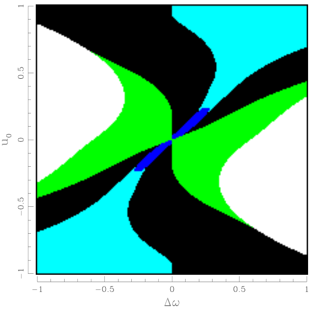
To illustrate the utility of the phase diagram approach, Figure 15 shows the results from time-evolving charge-perturbed coherent solutions with . Each pixel in the bitmap corresponds to a pair where a coherent solution with the given was perturbed by and time evolved until one of the conditions in Table 1 was met. For a coherent () solution to be considered stable, it must remain a bound state when subjected to both positive and negative charge perturbations ( and , respectively). For coherent solutions with , is positive and solutions are predicted to be unstable. It can clearly be seen that solutions are indeed unstable to like-charged perturbations and lead to PT end states (green pixels). Solutions with opposite-charged perturbations collapse but can lead to two different outcomes (BS or BH), depending on the amount of charge and the gravitational coupling. For most values of , the bubble walls begin to collapse, but the Coulombic self-repulsion leads to a bounce before the wall collapses to within the outer RN horizon and the solutions are modulated bound states (black pixels). For very small , on the other hand, the bubble walls do collapse to within the outer RN horizon and form black holes (blue pixels). For coherent solutions where , is negative and evolutions are predicted to be stable to perturbations. It can be seen that in this region that both positive and negative charge perturbations lead to bound states for the duration of the simulation, thereby indicating stable coherent solutions. For coherent solutions with , is positive and solutions are predicted to be unstable again; however this time, collapsing solutions end in dispersal and expanding solutions lead to modulated bound states without enough Coulombic self-repulsion to overcome the combined gravitational attraction and bubble wall surface tension.


Figure 16 shows twelve similar bitmaps, each covering the same range in space but for different values of gravitational coupling. With increasing gravitational coupling, more black holes appear, more perturbed solutions do not have initial data that can satisfy the boundary condition, and the number of bound states seems to decrease. The fact that the area of solutions in space supporting stable bound states reduces dramatically with increasing is indicative of the lack of stable bound states for gravitationally strong-field solutions. Figure 17 shows the transition across the boundary, above which no stable coherent bound states are observed. For these larger gravitational couplings, the range of values was adjusted to give insight into smaller perturbations, while a larger range of -space was used to clearly demonstrate the instability of solutions despite the stability condition being met.


Figure 18 shows finer detail of the phase diagram for . The aforementioned “triple point” can be seen around , where BH, PT, and BS solutions all exist in close proximity in space. Of particular interest is that near the triple point, a fractal structure is observed in the phase diagram. These solutions arise from “bounce” solutions that initially collapse but eventually bounce back and expand enough to become runaway PT solutions. Figure 19 shows these solutions colored based on the number of bounces (or modulations), , they undergo before inducing a runaway phase transition. This behavior is similar to the fractal boundary basins observed in real scalar field oscillon dynamics [34]. Figures 20 and 21 show the time evolution of the bubble radius for two different coherent solutions, and , for a variety of perturbations, . Figure 20 shows evolutions for three regions of the phase diagram. Region I is for , where all solutions induce a phase transition (the green region on the left side of the bitmap in figure 19). Region III is for larger , where all solutions collapse to form black holes (the blue region on the lower-right side of the bitmap in figure 19). Region II is the intermediate region, where BS or bounce (PT or BH) solutions are supported. Figure 21 shows time evolutions for bounce solutions like those in Region II of Figure 20, but for . Values of were chosen that demonstrate bounces prior to either inducing a phase transition or collapsing to a black hole.
Similar to behavior observed in oscillon dynamics [34], PT regions of space with modulations are surrounded by PT regions with modulations that approach the region with modulations in a log-periodic fashion. To demonstrate the log-periodic nature of the bounce regions, one first needs to find the boundary of such a region. Since a PT region with modulations is surrounded by either BS solutions or PT solutions with more than modulations, it is straightforward to vary and bisect on the boundary of the region, which is denoted . Figure 22 shows the result of bisecting on a boundary of a region. Approaching from within the region, all solutions (green line) are PT solutions, and a time-scaling law is observed as approaches ,
| (65) |
where is the nonuniversal scaling exponent. Approaching the boundary of the region from the other direction, one sees that regions of PT solutions approach the edge of the region in a log-periodic fashion. The time-minimum boundary of each band follows a time-scaling law with the same exponent. Between the bands, one can also see a rich structure of BS solutions and additional PT bands with (Figure 23). Both the bands and the structure between bands can be seen in Figure 24 to repeat in a discretely self-similar fashion,
| (66) |
where has been plotted for . While regular (i.e., not chaotic), this self-similarity in the set of PT solutions is fractal in nature because it has a nonintegral Minkowski-Bouligand dimension that depends on the width of and spacing between the bands in space, similar to [34].
IV.3 “Modest” Superextremal RN-AdS Solitons
It was shown in Section III that for the shape of potential () and charge coupling () used in this paper, super-extremal solutions exist for . Given that solutions with were observed to be unstable, one might naturally wonder whether the long-term fate of such superextremal solutions could be to collapse to form a naked singularity.
Because these solutions are bubbles with a true vacuum interior and a false vacuum exterior, local negative energy densities can be present inside these bubbles, and both the dominant energy condition and the weak energy condition can be violated and cosmic censorship does not necessarily hold. However, the only source of negative energy is from the scalar field potential, , and the amount of negative energy is proportional to the volume of space where . As such, if the bubble wall were to completely collapse, so would the volume of space that would contribute “negatively” to the local energy density. This would suggest that upon completely collapsing, the amount of negative energy arising from the true negative vacuum energy density would go to zero, the energy conditions could again be met, cosmic censorship would again hold, and naked singularities would not be present.
A more compelling argument can be made for the long-term “modesty” (lack of nakedness) of these solutions by considering the conservation of energy. Every evolution studied in this paper begins with perturbed bound-state initial data. The total matter, , is of finite extent, converges rapidly after , and is a conserved quantity. For the initial data with opposite-charged perturbations, the Coulombic self-repulsion is decreased and the bubble wall (and total mass) collapses inward. Unlike the subextremal case in which the bubble wall falls within the outer RN horizon, for this superextremal case there are no RN horizons and the formation of a naked singularity depends on whether the collapse continues indefinitely. Because the collapsing mass distribution is charged, one must consider the energy it takes to compress that charge against its own Coulombic self-repulsion. Complete collapse of the charged matter to a naked singularity would require an infinite amount of energy; this is analogous to the well-known infinite self-energy of a point charge. Because there is only a finite amount of energy, , that can be converted to electromagnetic mass-energy, and since there is a finite (and decreasing with radius) amount of negative energy from the true vacuum, the collapse must stop at some non-zero radius. Appendix B describes simple models describing the possible end-state of such a collapse and derives four different minimum radii based on different assumptions about the shape of the charge distribution.
Figure 25 shows the scalar field, geometry, and lapse function for a coherent solution with and , which has . Within the bubble wall radius (), the scalar field is approximately , the geometric variable can be seen to decrease from its value of unity at the origin (required by elementary flatness and regularity), and the lapse function can be seen to increase roughly linearly. As the solutions approach the bubble wall, the fields transition from their AdS values and match onto an RN exterior. Figure 26 shows the dynamics resulting from like-charged and opposite-charged perturbations of this solution. As expected, like-charged solutions form expanding bubbles that induce a phase transition, while opposite-charged solutions collapse.
To better understand the dynamics of collapsing superextremal solutions, it is helpful to understand the composite masses that contribute to the total ADM mass, . One can define
| (67) | |||||
| (68) | |||||
| (69) |
for the scalar potential, the electromagnetic field, and the gauge covariant derivative of the scalar field, respectively. One can see in Figure 27 that for this particular RN-AdS bubble solution, the magnitudes of and are many times larger than the magnitude of the total ADM mass, . The vacuum energy inside the bubble provides a very large negative energy contribution, approximately , while the gauge covariant derivative energy provides a very large (slightly larger in magnitude) positive energy contribution, approximately . The sum of these two terms is approximately , and the remaining mass, approximately , is mass-energy from the electromagnetic field. As the wall begins to collapse, begins to increase toward , and begins to decrease. Scalar field energy is being converted into electromagnetic energy because the fields are doing work by compressing the charge against Coulombic repulsion. Unfortunately, solutions become unstable around as a result of unphysical gauge shocks that arise from gauge radiation ( and ). The infalling radiative parts of the gauge potential do not contribute to but become severely compressed by the nearly collapsed lapse (), leading to steep gradients and code instability. Nevertheless, there is clear evidence that superextremal solutions with opposite-charged perturbations can collapse and result in strong-field gravitational solutions that match onto superextremal RN exteriors with nonsingular interiors.
V Conclusions
Results have been presented from numerical simulations of the EMH equations with a broken U(1) symmetry. Coherent nontopological solitons were shown to exist that separate a negative-energy AdS true vacuum interior () from a zero-energy RN false vacuum exterior (). The physical parameters (charge, mass, radius, and central lapse) of these solutions were obtained for a wide range of gravitational couplings. For , solutions are gravitationally strong-field solutions with radii on the order of their outer RN horizons and with central lapse function values of , indicating significant gravitational time dilation effects. For solutions with , the charge-to-mass ratios become superextremal (), the radii are , and the central lapse values are . Because obtaining these solutions requires fine-tuning to more than one part in , a 96-bit precision numerical code was used.
The stability of these solutions was tested by perturbing the charge of the coherent solution and evolving the time-dependent equations of motion. In the weak gravitational limit, the short-term stability depends on the sign of , similar to Q-balls. This condition does not hold, however, for and for . The long-term end-states of the perturbed solutions were visualized using “phase diagrams” that served as a way to clearly demonstrate regions of stability and instability. It was further demonstrated that there exists a rich fractal structure around the “triple point,” which was defined to be a region in the phase diagrams where BH, PT, and BS solutions exist in close proximity. The fractal structure results from bounce-like modulations of the scalar field where collapsing bubbles bounce back and induce phase transitions to the AdS true vacuum. The bands of modulations are surrounded by bands of modulations that approach the boundary of the modulation regions in a log-periodic manner. Threshold solutions are shown to demonstrate time-scaling laws with scaling exponents that depend on and total charge.
Finally, superextremal coherent RN-AdS solitons were shown to be unstable with an end state dependent on the sign of the charge perturbation. Like-charged perturbations led to expanding bubbles, and opposite-charged perturbations led to collapsing bubbles. While the superextremal charge-to-mass ratio might suggest a possibility of collapse to a naked singularity, it was shown that there is a minimum radius within which the wall can collapse based on the conversion of scalar field energy to electromagnetic energy. While it is still possible that solutions collapse and then bounce back to induce a phase transition, there is strong evidence supporting the existence of persistent nonsingular superextremal bound states that exhibit very strong-field gravitational behavior with . The existence of such solutions and their formation by decay of unstable coherent RN-AdS solitons was not previously known.
Appendix A Units and Dimensions
The action described in equation (1) was derived from the following dimensionful Lagrangian where :
| (70) | |||||
where is the characteristic boson mass, is Newton’s constant, and the are dimensionless.
Equation (1) is derived by transforming all the field variables and coordinates to dimensionless quantities according to the following transformations:
| (71) | |||||
| (72) | |||||
| (73) | |||||
| (74) |
which puts the Lagrangian in the following dimensionless form:
| (75) | |||||
| (76) |
where is dimensionless. Removing tildes in equation (75) results in equation (1).
Appendix B Minimum Radius of Gaussian Charge Distribution
This appendix discusses a simplified model of a collapsing charge distribution and uses the conservation of energy to derive the minimum radius to which the distribution can collapse. The charge density is assumed to be
| (77) |
which is normalized so that the total charge (enclosed) at infinity is . The charge enclosed for arbitrary is given by
| (78) | |||||
| (79) |
Integrating equation (26) from the origin to gives
| (80) | |||||
| (81) |
The mass-energy of the electromagnetic field is then given by
| (82) | |||||
Integrating the Hamiltonian constraint equation (28) yields the well-known equation for the geometry
| (84) | |||||
| (85) |
where is the total ADM mass,
| (86) |
and where is the mass-energy term arising from the covariant derivative of the scalar field, and is the mass-energy arising from the scalar field potential. For , the mass-energy of the electromagnetic field becomes
| (87) |
where the first term is the typical RN charge term, and the second term is a positive constant that can be considered the mass of the electromagnetic field at infinity, :
| (88) |
where
| (89) |
It should be stressed that the behavior of equations (87) and (88) is not valid because the assumption used to obtain the expression is violated in that regime. The -dependent terms are only proportional to and at large . The actual expression for the mass (82) is well behaved (approaches zero) as goes to zero.
The total mass of the field, however, does indeed go to infinity in the limit of small . This is consistent with the well-known infinite self-energy of a point charge. Nevertheless, the conservation of energy would imply that the final mass-energy of the electric field cannot exceed the total conserved ADM mass of the system:
| (90) |
which implies
| (91) |
which would set a limit on the collapse of the charge distribution.
While the minimum radius for a Gaussian-shaped charge density with mass is derived above, Table 2 presents the results of three additional models that all result in comparable minimum radii.
| Model Description | Constant () | |
|---|---|---|
| Gaussian | ||
| Linear | ||
| Constant | ||
| Constant , w/ approx. |
References
- [1] S. Coleman, Nucl.Phys.B, 262 263-283 (1985).
- [2] A. Kusenko, Phys.Lett., B404 285 (1997).
- [3] A. Kusenko, Phys.Lett., B406 26-33 (1997).
- [4] P. Jetzer and J.J. van der Bij, Phys.Lett.B, 227 341-346 (1989).
- [5] A. Cohen, S. Coleman, H. Georgi, and A. Manohar, Nucl.Phys.B, 272 301-321 (1986).
- [6] A.M. Safian, S. Coleman, and M. Axenides, Nucl.Phys.B, 297 498-514 (1988).
- [7] K. Lee, J.A. Stein-Schabes, R. Watkins, and L.M. Widrow, Phys.Rev.D, 39, 1665-1673 (1989).
- [8] K. Griest and E.W. Kolb, Phys.Rev.D, 40, 3231-3240 (1989).
- [9] J.A. Frieman, A.V. Olinto, M. Gleiser, and C. Alcock, Phys.Rev.D, 40, 3241-3251 (1989).
- [10] T.S. Levi and M. Gleiser, Phys.Rev.D, 66, 087701 (2002).
- [11] E. Palti,P.M. Saffin, and E.J. Copeland, Phys.Rev.D, 70, 083520 (2004).
- [12] T. Tamaki and N. Sakai, Phys.Rev.D, 86, 105011 (2012).
- [13] M. Gleiser and J. Thorarinson Phys.Rev.D, 73, 065008 (2006).
- [14] L. Pearce Phys.Rev.D, 85, 125022 (2012).
- [15] F.P. Correia and M.G. Schmidt, Eur.Phys.J., C21 181-191 (2001).
- [16] K.N. Anagnostopoulos, M. Axenides, E.G. Floratos, and N. Tetradis, Phys.Rev.D 64, 125006 (2001).
- [17] X. Li, J. Hao, and D. Liu, J.Phys.A 34, 1459 (2001).
- [18] M. Deshaies-Jacques and R. MacKenzie, Can.J.Phys. 85, 693 (2007).
- [19] H. Arodz and J. Lis, Phys.Rev.D 79, 045002 (2009).
- [20] I.E. Gulamov, E.Ya. Nugaev, and M.N. Smolyakov, Phys.Rev.D 89, 085006 (2014).
- [21] T. Tamaki and N. Sakai, Phys.Rev.D, 84, 044054 (2011).
- [22] N. Sakai and T. Tamaki, Phys.Rev.D, 85, 104008 (2012).
- [23] T. Tamaki and N. Sakai, Phys.Rev.D, 90, 085022 (2014).
- [24] B. Kleihaus, J. Kunz, and S. Schneider, Phys.Rev.D, 85, 024045 (2012).
- [25] N. Sakai and M. Sasaki, Prog.Theor.Phys., 119 929-937(2008).
- [26] T. Tamaki and N. Sakai, Phys.Rev.D, 83, 044027 (2011).
- [27] R.J.W. Petryk, Ph.D. thesis, The University of British Columbia, 2005.
- [28] M. Gleiser, Phys.Rev.D, 38, 2376-2385 (1988).
- [29] T. Tamaki and N. Sakai, Phys.Rev.D, 81, 124041 (2010).
- [30] M. Kawasaki, K. Konya, and F. Takahashi, Phys.Lett., B619, 233-239 (2005).
- [31] S.L. Liebling and C. Palenzuela, Living Rev. Relativity 15, lrr-2012-6, (2012).
- [32] E.P. Honda and M.W. Choptuik, Phys.Rev.D, 65, 084037 (2002).
- [33] E.J. Copeland, M. Gleiser, and H.R. Müller Phys.Rev.D, 52, 1920-1933 (1995)
- [34] E. Honda, Phys.Rev.D, 82, 024038 (2010).
- [35] U. Nucamendi and M. Salgado, Phys.Rev.D, 68, 044026 (2003).
- [36] M. Alcubierre, J.A. Gonzalez, and M. Salgado, Phys.Rev.D, 70, 064016 (2004).
- [37] M. Bucher, Phys.Lett.B, 530, 1-9 (2002).
- [38] IEEE, IEEE Std 754–2008, (2008).