Hierarchical data-driven approach to fitting numerical relativity data
for nonprecessing binary black holes with an application to final spin and radiated energy
..LIGO document number: LIGO-P1600270-v5
Abstract
Numerical relativity is an essential tool in studying the coalescence of binary black holes (BBHs). It is still computationally prohibitive to cover the BBH parameter space exhaustively, making phenomenological fitting formulas for BBH waveforms and final-state properties important for practical applications. We describe a general hierarchical bottom-up fitting methodology to design and calibrate fits to numerical relativity simulations for the three-dimensional parameter space of quasicircular nonprecessing merging BBHs, spanned by mass ratio and by the individual spin components orthogonal to the orbital plane. Particular attention is paid to incorporating the extreme-mass-ratio limit and to the subdominant unequal-spin effects. As an illustration of the method, we provide two applications, to the final spin and final mass (or equivalently: radiated energy) of the remnant black hole. Fitting to 427 numerical relativity simulations, we obtain results broadly consistent with previously published fits, but improving in overall accuracy and particularly in the approach to extremal limits and for unequal-spin configurations. We also discuss the importance of data quality studies when combining simulations from diverse sources, how detailed error budgets will be necessary for further improvements of these already highly accurate fits, and how this first detailed study of unequal-spin effects helps in choosing the most informative parameters for future numerical relativity runs.
I Introduction
According to general relativity, compact binary black holes (BBHs) coalesce through the emission of gravitational waves (GWs), as already observed by LIGO in at least two cases [1, 2, 3, 4]. The merger remnant is a single Kerr BH [5] characterized only by its final spin and mass. An essential and robust tool for predicting BBH evolution, since the 2005 breakthrough [6, 7, 8], is numerical relativity (NR). Due to the large computational cost of each NR simulation, it is still computationally prohibitive to cover the BBH parameter space exhaustively. Hence it is natural to develop simple, yet accurate model fits to the existing set of NR simulations. One then has to study their quality of interpolation between NR simulations, and of extrapolation to regions of parameter space beyond the calibration range. For example, the phenomenological inspiral-merger-ringdown waveform models of [9, 10, 11, 12, 13], though used very successfully as one of two waveform families for LIGO O1 data analysis [1, 2, 3, 4], still include only a limited set of physical effects and were calibrated to small sets of NR simulations with relatively simple fitting methods.
In this paper we develop a more general, hierarchical fitting approach for BBH properties and waveforms. The fit ansatz functions are developed through studying hierarchical structures present in the NR data set itself, and their complexity tailored to the actual predictive power of the data set by the use of information criteria.
We first apply this method to the spin and mass of the remnant black hole, which determine the frequencies of the quasinormal-mode ringdown [14, 15, 16, 17] to a Kerr black hole. The ringdown is a crucial part in modeling full inspiral-merger-ringdown waveforms [18, 9, 10, 11, 12, 13, 19, 20]; and from parameter estimation with the full waveforms, the final mass and spin can be estimated with accuracy similar to other BBH parameters [2, 4]. Future observations of strong GW signals will allow to test general relativity through consistency tests between inspiral, merger and ringdown [21], significantly improving upon [22].
Apart from GW observations, the final state of a BBH merger is astrophysically interesting in itself, e.g. for the computation of merger trees [23, 24, 25, 26, 27, 28, 29, 30]. The mass and spin of BHs surrounded by matter, e.g. accretion disks, may also be inferred from electromagnetic observations (see [31, 32] for stellar-mass BHs and [33, 34, 35] for supermassive BHs).
For this paper, we concentrate on nonprecessing quasicircular BBHs, where the black hole spins are parallel or antiparallel to the total orbital angular momentum of the binary. These configurations are fully described in a three-dimensional parameter space: given the masses and physical spins , we use the two component spins and and the mass ratio, given either as with the convention , or as the symmetric mass ratio . The total mass is only a scaling factor, and here we work in units of .
As suggested by the post-Newtonian (PN) results [36, 37, 38, 39] for radiated energy and angular momentum, and confirmed by many previous studies of NR-calibrated models [18, 40, 41, 9], the two dominant parameter dependencies of both final spin and final mass are on the mass ratio and on some appropriately chosen effective spin parameter of the binary, whereas the effects of any difference between the two individual spins are much smaller. However, only by accurately modeling these small unequal-spin effects can the full two-spin information be extracted from GW observations, disentangling any true physical degeneracies from systematic effects due to limitations of the waveform models.
A similar, but more complex, situation is encountered in the calibration of phenomenological models to precessing binaries, where so far a simple waveform model based on a single effective precession parameter [11, 12, 13] has successfully been employed to analyze the first gravitational wave detections [2, 4]. (A complementary precessing analysis [42] based on the model of [20, 43] has also been published recently.) The current work, while mainly a first step to develop models for the full three-dimensional parameter space of nonprecessing waveforms, can also be considered as a toy model for the numerical calibration of subdominant effects in generic binaries, such as precession and higher modes.
For the current three-dimensional aligned-spin parameter space, in addition to the hierarchy of mass ratio, effective spin and spin difference, the sampling by available NR simulations still displays significant bias toward simple subsets: namely the one-dimensional subspaces of nonspinning cases ( dependence only) and equal-mass, equal-spin cases (, , , thus effective-spin dependence only) are covered particularly well by existing NR catalogs, while few simulations exist for unequal spins, high spins, and/or very unequal masses. Independently, the extreme-mass-ratio limit (, , arbitrary spins) is known analytically [44].
Here we exploit and investigate this structure by parametrizing spin effects in terms of an effective spin and a spin-difference parameter. As the effective spin we choose
| ((1)) |
which has already been found to work well for final-state quantities in [9]. We discuss other possible choices for the effective spin, for which our method also works robustly, in Appendix C. For spin difference, we use simply , which makes no assumptions on how spin-difference effects depend on mass ratio.
We develop our hierarchical approach, with the aim to ensure an accurate modeling of the subdominant spin-difference effects, along the lines illustrated as a flowchart in Fig. 1: First we consider the one-dimensional subspaces of nonspinning and of equal-mass-equal-spin black holes. We then combine and generalize these subspace fits, adding additional degrees of freedom to cover the entire two-dimensional space of equal-spin black holes, but constrain the generalized ansatz with information from the extreme-mass-ratio limit. In a third step, we investigate the leading subdominant terms, which are linear in the difference between spins, and also identify additional nonlinear spin-difference terms. We finally produce a three-dimensional fit to the complete data set with the hierarchically constructed ansatz. This way, we can construct a full ansatz with a relatively low number of free fit coefficients and avoid overfitting of spurious effects only due to small sample sizes, while still capturing the essential physical effects that are known from the well-constrained regions.
At each step, we evaluate the performance of different fit choices by several quantitative measures: by the overall residuals, by the Akaike and Bayesian information criteria (AICc, BIC, [45, 46]), and by how well determined the individual fit coefficients are. The information criteria are model selection tools to choose between fits with comparable goodness of fit but different degrees of complexity, i.e. they penalize high numbers of free coefficients. See Appendix B for details on these statistical methods.
Previous published fits for final spin and/or mass include [47, 48, 49, 27, 50, 51, 52, 9, 53, 54, 55], and we will compare our results to the most recent results in the literature, including both fits across the full three-dimensional nonprecessing parameter space, and the effective-spin-based fits from [9], which were used in the aligned-spin IMRPhenomD waveform model [9, 10] and (with in-plane-spin corrections) in the precessing IMRPhenomPv2 model [11, 12, 13]. These will be referred to as the “PhenomD fits” in the following. The plan of the paper is as follows: We first describe our data sets, built from several NR catalogs, in Sec. II, together with the available extreme-mass-ratio limit information. In Sec. III we develop the general fitting recipe for the example of the final spin. We then apply our method also for final mass – or equivalently, radiated energy – in Sec. IV, which illustrates some of the specific choices and adaptations required to apply the general method to each quantity. We summarize our method and results in Sec. V, and give additional details about NR data, fit construction, and fit uncertainty estimates in Appendices A–D.

Our fits for final spin and radiated energy are also provided in Mathematica and python formats as supplementary material [56, *Jimenez-Forteza:2016oae-anc], and implemented under the label “UIB2016” in the nrutils.py package of LALInference [58, 59]. This final version of the paper uses a larger NR calibration set than the initial arXiv submission (1611.00332v1), with fit results fully consistent but better constrained.

II Input data
II.1 Numerical Relativity data sets
We combine four data sets of aligned-spin numerical relativity BBH simulations from independent codes and sources: the public catalogs of SXS [60, 61], RIT [52, 62] and GaTech [63, 64]; as well as a set of our own simulations with the BAM code [65, 66, 9], including 27 new cases for which initial configurations and results are listed in Table 14 in Appendix A. After removing 16 cases from the combined data set due to data quality considerations as discussed in Appendix A, we have 161 cases from the SXS catalog, 107 from RIT, 114 from GaTech and 45 from BAM; for a total of 427 cases. The sampling of our three-dimensional parameter space by the four data sets is shown in Fig. 2. The initial arXiv version of this paper (1611.00332v1) used a smaller data set of 256 NR cases, with the increase coming from an update of the public SXS catalog and new RIT results from [62].
To obtain a qualitative understanding of the hierarchical structure in the two-dimensional parameter space of mass ratio and effective spin, in Fig. 3 we show the NR data set over the plane together with the analytical extreme-mass-ratio results, discussed below in Sec. II.2. For both final spin and radiated energy, we find a reasonably smooth surface spanned by the NR data points. These plots already suggests that – together with the known extreme-mass-ratio results to compensate the sparsity of NR simulations at increasingly unequal masses – good one-dimensional fits in the two best-sampled one-dimensional subsets (equal-mass-equal-spin and nonspinning BHs) will significantly constrain any two-dimensional fits.
Furthermore, as a first quantitative check that the assumption of a hierarchical structure in three-dimensional BBH parameter space holds, with unequal-spin effects subdominant to the dependence on and , we can study the residuals of this data set under the two-dimensional PhenomD fits [9]. For final spin, we find that 90% of relative errors are below 3%. (The only cases over 10% are those with absolute values close to zero, where relative error is not a good measure, and absolute errors (residuals) are limited to .) Still, this comparison suggests that unequal-spin effects make a large contribution to these small errors, as shown by four times smaller 90% quantiles when restricting to equal-spin cases only. See also Fig. 4 for histograms of these distributions. For radiated energy, 90% of relative errors are below 2%, with a reduction of that quantile by 1.4 for equal-spin cases only, indicating that spin-difference effects are even smaller for this quantity, which we will also see confirmed in our final results.

For details about extraction of final-state quantities, NR data quality and weight assignment, see Appendix A. As explained there, we do not have a full set of NR error estimates available, so we assign heuristic fit weights to each case based on the expected accuracy of the respective NR code in that particular parameter space region. For example, high-mass-ratio cases are down-weighted more for puncture codes.
II.2 Extreme-mass-ratio limit
The computational cost of numerical simulations of BH binaries in full general relativity diverges in the extreme-mass-ratio limit . However, this limit is also equivalent to the much simpler case of a test particle orbiting a Kerr black hole. The energy and orbital angular momentum for that configuration have long been known analytically [44]: inserting the radius of the innermost stable circular orbit (ISCO) from Eq. (2.21) of [44] into Eqs. (2.12) and (2.13) of the same reference yields the test-particle energy (equivalent to the radiated energy) and orbital angular momentum at ISCO:
| ((2)a) | |||||
| ((2)b) | |||||
with
| ((3)a) | |||||
| ((3)b) | |||||
| ((3)c) | |||||
Note that both and depend linearly on .
In the test-particle limit, the small BH plunges after reaching the ISCO, and further mass loss scales with [67]. Similar to previous work [68, 47, 52, 55], we will exploit this fact to compute the final spin and radiated energy to linear order in from the analytical expressions, Eq. (2), holding at the ISCO. To linear order in , we thus simply have or for the final mass, and for the final spin we obtain the implicit equation
| ((4)) |
where the individual BH spins can be written in terms of our effective spin as
| ((5)) |
Equation (4) can then be solved numerically for the final spin as a function of and of the effective spin . Since this result holds to linear order in , and assuming that the final spin and mass are regular functions of , we have thus essentially computed the derivatives and at , in addition to the values at , which are and .
Additionally, assuming that the final state is indeed a Kerr BH, its final spin has to satisfy . One would also expect the final spin for maximal effective spin, , to decrease monotonically with increasing . To construct an accurate fit in a neighborhood of that satisfies these expectations – in particular the Kerr limit – we will constrain our ansatz with the analytically computed value of at . By perturbing Eq. (4) around to linear order before taking the derivative in at the same point, we find
| ((6)) |
Several variations of this procedure have been used for previous final-spin fits, and differences are due to previous works neglecting the radiated energy in Eq. (4) [47, 52], or not enforcing the derivative for satisfying the Kerr limit [55].
III Final spin
We will now first develop the details of our hierarchical fitting procedure for the example of the final spin of BBH merger remnants, giving more detail here than we will do for the radiated energy in Sec. IV.
III.1 Choice of fit quantity
We first need to decide which quantity exactly we want to fit. It appears natural to fit a quantity related to the “final” orbital angular momentum near merger, i.e. separating out the known initial spins . This is particularly useful in connection with the extreme-mass-ratio limit, since with Eq. (2)b, is linear in to leading order. We can use the relation from Eq. (4) between and the dimensionless Kerr parameter of the remnant BH, , also outside the extreme-mass-ratio limit. Here is the final mass of the remnant BH.
Instead of the actual angular momentum , we take the liberty of fitting the quantity , where (as throughout the paper) is set to unity. This way, all fit results are easily converted to the final Kerr parameter by adding the total initial spin , and no correction for radiated energy has to be applied.
III.2 One-dimensional subspace fits
Motivated by the the unequal sampling of the parameter space by NR simulations, as visualized in Fig. 3, we start our hierarchical fit development with the simplest and best-sampled subspaces of the NR data set, constructing one-dimensional fits and over 92 nonspinning and 37 equal-mass-equal-spin cases. We do not restrict ourselves to polynomial fits, and also include ansätze in the form of rational functions. We have also found good fits for more general functions, but omit these here since we have not explored that option systematically.
All fits are performed with Mathematica’s NonlinearModelFit function, but also partially cross-checked with the nls package of R. Since rational functions can have singularities, codes such as NonlinearModelFit may not converge to a valid solution without good starting values for the coefficients. We solve this problem by first performing a sufficiently high-order polynomial fit, from which we compute a Padé approximant at the desired order, and use the coefficients of this approximant as starting values for the rational-function fit. We denote rational functions with a numerator of polynomial order and denominator of polynomial order as an ansatz of order . Before fitting to the NR data, all ansätze are constrained by two facts: For nonspinning BBHs, both and have to vanish for , so that there can be no constant term in the ansatz. Furthermore, from the extreme-mass-ratio prediction Eq. (2), it also follows that the spin-independent coefficient linear in is (see also [69]). We will include spin-dependent information linear in in Sec. III.3.
Thus, we obtain fits for a large set of polynomial and rational functions. Several of them produce competitive goodness of fit, as measured by the root-mean-square-error (RMSE) or the full distribution of residuals. However, we do not want to overfit the data, which could induce spurious oscillations in the region of very unequal BH masses that is not covered by NR data. Hence, we rank the fits by information criteria penalizing superfluous free coefficients.

| Estimate | Standard error | Relative error [] | |
|---|---|---|---|

| Estimate | Standard error | Relative error [] | |
|---|---|---|---|
Figure 1 shows the top-ranked fit in terms of Schwarz’s Bayesian information criterion (BIC), which is a rational function of order (3,1):
| ((7)) |
The fit coefficients along with their uncertainties are given in Table 1; all are well determined. The exact ranking of fits can depend on the choice of fit weights (see Appendix A) and on the ranking criterion, but we find that Eq. (7) is top-ranked by both BIC and AICc. While only ranked 6th by RMSE, none of the considered fits is better than Eq. (7) by more than 6% in that metric either. Additionally, under variations of the weighting scheme, this is robustly the fit among the top-ranked group – by all three criteria – with the lowest number of fitting coefficients, indicating it is a robust choice. For comparison, a simple third-order polynomial (two free coefficients) is disfavored clearly, by more than a factor of 8 in RMSE and an offset of +452 in BIC, and a fourth-order polynomial (three free coefficients, just as Eq. (7)) by almost a factor of 2 and by +332 respectively.
The lower panel of Tbl. 1 also compares the preferred fit both to the NR data and to the three next-best ranking fits by BIC. We find that the residuals are centered around zero with no major trends, while the differences among high-ranked fits are much smaller than the scatter of residuals for the well-covered high- range, and that the “systematic uncertainty”, as indicated by the difference of high-ranked fits, is still at the same level even in the extrapolatory low- region. The BIC ranking for this example is also illustrated in Fig. 29 in Appendix B.
Before the second 1D fit in the effective spin parameter , we need to decide how we are later going to construct a 2D ansatz combining both 1D fits. We can either subtract or divide the NR data by the nonspinning fit, and find that subtraction exhibits a simpler functional form. Thus we decide to construct a 2D ansatz as the sum of nonspinning and spinning contributions. (We will choose a product ansatz for the radiated energy discussed in the next section.) We thus constrain the constant term of the 1D ansatz in to reproduce the nonspinning result, i.e. must be identical for both 1D fits.
The top-ranked fits by BIC are shown in Tbl. 2, and again we find a unique top-ranked fit by both AICc and BIC, a rational function of order (3,1):
| ((8)) |
with four fit coefficients as listed in Table 2. This ansatz is ranked 8th by RMSE, but with only 3% difference from the lowest RMSE, which is attained by a P(5) fit with one more coefficients, marginally disfavored by about +1.7 AICc and +2.6 in BIC. The best three-coefficient fit R(2,1) is significantly worse, with differences of over +40 in BIC/AICc and 40% in RMSE. Again, the distribution of residuals is well behaved, and differences between the four top-ranked fits by BIC are smaller than the scatter of residuals.

| Estimate | Standard error | Relative error [] | |
|---|---|---|---|
III.3 Two-dimensional fits
Next, we want to construct a two-dimensional fit covering the space, as it was illustrated in Fig. 3, by combining both the 1D subspace fits and the extreme-mass-ratio limit. As discussed above, we take the sum of Eq. (7) and the spin-dependent terms of Eq. (8). We introduce the necessary flexibility to describe 2D curvature and the extreme-mass-ratio limit by generalizing the -dependent terms, inserting a polynomial of order in for each through the substitution
| ((9)) |

The general 2D ansatz is thus
| ((10)) |


Here we choose to expand to third order in (), which is the lowest order leaving enough freedom to incorporate all available constraints from the 1D fits and the extreme-mass-ratio limit, and, as evidenced by the residuals we find below, also high enough to adequately model this data set. Of the resulting 16 coefficients, the three in the numerator must vanish to preserve the limit, while consistency with the equal-mass fit from Eq. (8) provides four constraints which we use to fix the terms:
| ((11)) |
Four more coefficients are fixed by the extreme-mass-ratio information discussed in Sec. II.2: we re-express Eq. (4) in terms of and fit the discretized quantity
| ((12)) |
where is the linear contribution from the nonspinning part (cf. Eq. (7)) and the values are obtained by solving Eq. (4) numerically for small . Before fitting, we apply the derivative constraint from Eq. (6), which for the sum ansatz Eq. (10) implies a coefficient constraint
| ((13)) |
We find this extra physical constraint to be essential in avoiding superextremal results due to fitting artifacts. The extreme-mass-ratio limit fit coefficients are listed in Table 3, and the improved agreement between analytical results and this new fit, as compared with the previous fit of [9], is illustrated in Tbl. 3.
In summary, after constraining to the well-covered one-dimensional NR data subsets and the analytically known extreme-mass-ratio limit, the 2D ansatz from Eq. (10) has reduced from 16 to 5 free coefficients. We fit it to the 60 remaining equal-spin NR cases that were not yet included in the 1D subsets. To remove possible singularities in the plane for this rather general rational ansatz, we set the least-constrained denominator coefficient to zero. Thus we obtain a smooth four-coefficient fit as shown in Fig. 8. It has RMSE four times larger than the 1D fit and twice as high as the fit, but these residuals are still smaller than expected unequal-spin effects and rather noisily distributed without any clear parameter-dependent trends, thus indicating that the 2D fit sufficiently captures the dominant dependence to form the basis of studying subdominant spin-difference effects. The least-constrained coefficient at this point has a relative error of about 25%, which is good enough to keep it in the ansatz for the next, 3D step where we will refit to a larger data set.
III.4 Unequal-spin contributions and 3D fit


Now the final step in the hierarchical procedure is to explore the subdominant effects of unequal spins, parametrized by the spin difference . We first study the residuals of the 238 unequal-spin NR cases under the equal-spin 2D fit:
| ((14)) |
We do this at fixed steps in mass ratio, having sufficient numbers of NR cases for this analysis at mass ratios . This per-mass-ratio analysis is only used to guide the construction of the full 3D ansatz and as a consistency check, while the final full 3D fit will consist of fitting the constrained 2D ansatz plus spin-difference terms directly to the full data set.
At each mass ratio, we visually inspect the residuals, which span 2D surfaces in or, equivalently, space. As illustrated in Fig. 9, we find surfaces close to a plane, indicating a dominant linear dependence on and possibly a mixture term . The exception is at equal masses, where quadratic curvature in the dimension dominates. In this case, exchange of and yields an identical binary configuration, so that terms linear in indeed have to vanish. We have also exploited this fact in the analysis by adding mirror duplicates of each NR data point. Motivated by these empirical findings and symmetry argument, we introduce up to three spin-difference terms,
| ((15)) |
The full 3D ansatz is then simply the sum of Eqs. (10) and (15):
| ((16)) |
Adding higher orders in the effective spin or spin difference is not supported by visual inspection. At each mass ratio, we now perform four fits in for the values of the : linear, linear+quadratic, linear+mixed, or the sum of all three terms. Examples are also shown in Fig. 9.
We then collect the coefficients of each of these fits and use them as data to be fitted as functions of mass ratio (see the ’per-mass-ratio data’ in Fig. 10), using as weights the fit uncertainty from each mass ratio rescaled by the average data weight for that mass ratio. We also apply what we know about the extreme-mass-ratio and equal-mass limits: all three have to vanish in the limit , and the , linear in have to vanish for . We thus choose ansätze of the form
| ((17)) |
for linear in , where the factor is motivated from post-Newtonian (PN) results [38, 39], and
| ((18)) |
for the term quadratic in . We find that the data can be well fit without any higher-order terms and by reducing some of the freedom of these three terms exploratory fits keeping all coefficients free give results close to integer numbers for the , and . Hence we choose the three parsimonious ansätze
| ((19)a) | ||||
| ((19)b) | ||||
| ((19)c) | ||||
The blue points and lines in Fig. 10 show these per-mass-ratio results. The shape and numerical results of the dominant linear term are quite stable under adding one or two of the other terms. Fitting two terms, either linear+quadratic or linear+mixture, yields quadratic/mixture effects of very similar magnitude, with the quadratic term following the same basic shape (an intermediate-mass-ratio bulge) as the other two. However, combining all three terms, the results match better with the expectations from symmetry detailed before, with the bulge shape limited to the linear and mixture terms while the quadratic term provides a correction mostly at similar masses.
Using again the , and constraints on the general ansatz from Eq. (16), we end up with a total of nine free coefficients in this final step. We now fit to 298 cases with arbitrary spins not yet used in the 1D fits, with results given in Table 4. Together with the coefficients from Tables 1–3, these fully determine the fit. To convert back from our fit quantity to the actual dimensionless final spin , just add the total initial spin .
| Estimate | Standard error | Relative error [] | |
|---|---|---|---|
We find that the data set is sufficiently large and clean, and the equal-spin part modeled well enough from the 2D step, to confidently extract the linear spin-difference term and its -dependence, which is stable when adding the other terms; and to find some evidence for the combined mixture and quadratic terms, whose shape however is not fully constrained yet.
III.5 Fit assessment
In Fig. 10 we also compare the spin-difference terms from this final “direct 3D” fit to those obtained from the per-mass-ratio residuals analysis. The linear term is fully consistent, confirming that it is well determined by the data, while for the quadratic and mixture terms both approaches agree on the qualitative shape, but do not match as closely. Under the chosen ansätze, the 3D fit coefficients even for those terms are tightly determined (see Table 4). However, we have explicitly chosen the spin-difference terms in Eq. (19) to achieve this goal, while several other ansatz choices (changing the fixed exponents of the multiplicative or terms, or adding more terms with free coefficients in the polynomials) can produce fits that are indistinguishable by summary statistics (AICc, BIC, RMSE). Still, most of these have some strongly degenerate and underconstrained coefficients, while the reported fit has the desirable property of sufficient complexity to be within the plateau region of summary statistics while not having any degenerate coefficients.
Yet, the shape of the functions and for the mixture and quadratic terms is not actually as closely constrained from the current data set as the coefficient uncertainties alone seem to imply, due to this ambiguity in ansatz selection. This becomes clear from the comparison of direct 3D fit and per-mass-ratio analysis in Fig. 10. The per-mass-ratio analysis also demonstrates that the data at mass ratios are not yet constraining enough to help characterize these terms. (The error bars are so large, and hence the weights so low, that they effectively do not contribute to the fit.) It also becomes clear that additional unequal-spin data at intermediate mass ratios would be very useful in constraining the functions. Meanwhile, it is important to note again that the leading linear spin-difference term is already determined much more narrowly and robustly with the current data set.
We can further assess the success of the hierarchical 3D fitting procedure by comparing
- •
a 2D fit (equal-spin physics only) to equal-spin NR cases only (same as in Fig. 8),
- •
a 2D fit (equal-spin physics only) to all NR data,
- •
and the 2D part of the full 3D fit.
As shown in Tbl. 5, fitting the 2D equal-spin ansatz to the full data set induces strong curvature in the plane, which the full 3D fit is able to correct by the additional degrees of freedom in the spin-difference dimension. This is how it was possible to pull out the subdominant spin-difference effects with this enlarged data set. The same conclusion is supported by the comparison of summary statistics between the various steps and 2D/3D fit variants in Table 5, showing that the RMSE only increases by 50% from the 2D equal-spin case to the full 3D fit using all data.

Orange: Difference of the 2D part of the 3D fit to the full data set minus the 2D-only fit to equal-spin data. The bulk of the parameter space is no longer distorted, and only at high effective-spin magnitudes a small opposite effect to the -dependent behavior of the spin-difference terms (cf. Fig. 10) can be seen.
| RMSE | AICc | BIC | |||
|---|---|---|---|---|---|
| 1D | |||||
| 2D all | |||||
| 3D lin | |||||
| 3D lin+quad | |||||
| 3D lin+mix | |||||
| 3D lin+quad+mix |


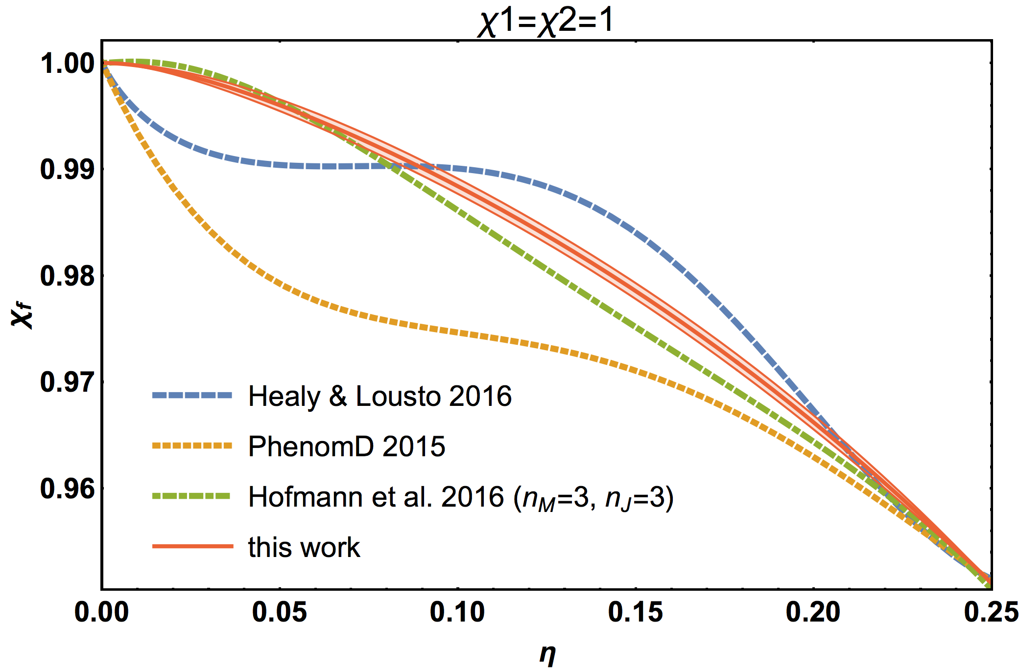
The distribution of fit residuals for the full data set, projected onto the plane, is shown in Tbl. 6, and a comparison of fit residuals with other previously published fits, over the calibration data set of the current work, is shown as histograms in Tbl. 6 and summarized in Table 6 along with AICc and BIC metrics. The shape of the distributions is consistent, and for all fits the means are much smaller than the standard deviations, showing no evidence for any systematic bias. Our new fit improves significantly over the previous fit [9] used in the calibration of the IMRPhenomD waveform model [10], and also yields some improvement over recent fits from other groups [62, 55], even when those ansätze are refit to our present NR data set.
Refitting our final hierarchically obtained ansatz directly to the full data set produces slightly better summary statistics, but also allows uncertainties from the less well-controlled unequal-spin set to influence the other parts of the fit, while the stepwise fit gives better control over the extreme-mass-ratio behavior and better-determined coefficients for the well-constrained subspaces.
As a further test of robustness, we have repeated the hierarchical fitting procedure with uniform weights instead of the weights used so far and discussed in Appendix A. This yields a fit consistent with our main result, though slightly less well constrained, but still improving over previous fits, thus demonstrating the robustness of the hierarchical fit construction under weighting choice.
We have also verified that our new fit does not violate the Kerr bound, particularly in the extreme-spin limit () and at low , see Fig. 14.
III.6 Precessing binaries
While some existing final-spin fits [53, 54, 55] also include a calibration to precessing cases, it is also possible to use a simple “augmentation” procedure [49] (see also [68]) for aligned-spin-only calibrations by adding the contribution of in-plane spins in quadrature to the aligned-spin fit result:
| ((20)) |
This procedure is known to significantly improve accuracy and reduce bias for precessing binaries. For example, it has been applied to the aligned-spin PhenomD fit [9] for the precessing PhenomPv2 model [12, 13], and to the RIT fit [52] in recent parameter estimation work of the LIGO-Virgo collaboration [4, 70, 42] (including spin evolution according to [41]).
Applying Eq. (20) to our aligned-spin fit, we find a small overshooting of the Kerr bound for mass ratios , when the spin magnitude of the heavier BH is very close to extremal, and for certain orientation angles of the black holes’ spins to the angular momentum. The worst cases give an excess in of about 0.12% at and intermediate opening angles, comparable to the aligned-spin fit residuals. No overshooting occurs if only the linear-in- term in the final spin is used. Such a small inaccuracy when extending the aligned-spin fit to precessing cases is in principle not surprising, as this parameter-space region is not covered with NR simulations and hence the fit slope in this region is purely determined by extrapolation between the NR data and the extreme-mass-ratio limit, which we have ensured to be smooth with a flat approach to at (see Sec. II.2 and Fig. 14). Very small inaccuracies in the intermediate- extrapolation region can thus lead to a minimal Kerr violation when adding the in-plane spins according to Eq. (20). A clean solution to this issue would require more calibration NR simulations in the critical region and a study of precessing spin contributions in the extreme-mass-ratio limit.
However, as the overshooting is very small, we have investigated two easy ad hoc solutions: We could take the worst-case point and enforce our 3D fit to be at or below the corresponding value for the aligned-spin projection by putting a constraint on one of the coefficients. This can remove the overshooting at the worst-case point and nearby, but not over the whole problematic region, as the fit still has enough freedom in other parameters. But the accuracy of the aligned-spin fit already suffers from this one extra constraint, and using constraints on more than one coefficient to pull down the augmented over a wider parameter region is fully prohibitive because insufficient freedom will remain in the fit to properly calibrate to the actual NR data.

| Estimate | Standard error | Relative error [] | |
|---|---|---|---|

| Estimate | Standard error | Relative error [] | |
|---|---|---|---|
Hence, we opt for an even simpler solution, truncating the augmentation from Eq. (20) at unity: . This is justified as the overshooting is very small, on the order of the fit residuals, and limited to an extremal parameter-space region. The need for this ad hoc truncation will reduce or become obsolete when low--high-spin NR simulations and/or precessing extreme-mass-ratio information become available. A detailed comparison of fit accuracies over a representative set of precessing NR runs is left to future work.
IV Final mass and radiated energy
To fit the final mass of remnant BHs from BBH mergers, we use the same hierarchical approach as for the final spin, summarized in Fig. 1, with only minor modifications. The quantity we are going to fit here is the dimensionless radiated energy, . For , it has to vanish even in spinning cases, while the analytical expectation for the leading order in , as , is . We construct the two-dimensional ansatz as a product of the 1D ansätze, instead of a sum as in the final-spin case.
In principle, the fitting procedure is robust enough to use either a sum or product ansatz for either final-state quantity. Actually, by carrying out the full procedure for as described in the following subsections, but using a sum of the 1D contributions, we found a fit statistically at least competitive with that obtained from a product. However, in this case the sum ansatz tends to produce suspicious curvature in the , low- region, which cannot be suppressed by the extreme-mass-ratio information. With additional NR data in this region, that problem might be alleviated, but with the current data set we find the product ansatz to be more robust and able to yield a final fit that is both accurate and well determined over the calibration region and without obvious bad behavior in extrapolation.
IV.1 One-dimensional fits
For the nonspinning 1D fit in symmetric mass ratio , a simple fourth-order polynomial
| ((21)) |
with three free coefficients, listed in Table 7, is marginally preferred by both AICc and BIC. More complicated rational functions are not able to yield any significant change in residuals (only up to 1% in RMSE), while the differences between Eq. (21) and the next-ranked fits are again much smaller than the remaining residuals, as shown in Tbl. 7.
For the effective-spin dependence, again the value at is fixed from the fit. A rational function of order (3,1) is top-ranked by AICc, BIC and RMSE and thus unambiguously selected as the preferred ansatz:
| ((22)) |
with four free coefficients listed in Table 8, and well-behaved residuals as seen in Tbl. 8.
IV.2 Two-dimensional fits

| Estimate | Standard error | Relative error [] | |
|---|---|---|---|

For the 2D ansatz, we combine the two 1D fits from Eqs. (21) and (22), expanding each -dependent term with a polynomial in , according to Eq. (9), and removing the value from the spin ansatz before multiplying with the terms:
| ((23)) |
Contrary to the sum ansatz for in Eq. (10), we do not need to set the -independent coefficients of the terms to zero, as the form of Eq. (23) already guarantees the correct limit. Hence an expansion up to third order in of each term, as we chose for the fit, would yield too many free coefficients, and instead we only expand up to second order. The four coefficients are again fixed by the equal-mass boundary conditions:
| ((24)) |
Similar to the procedure for , we can use the extreme-mass-ratio limit to fix the four coefficients of the linear-in- terms. Using the analytic result from Eq. (2)a, we force the fit to satisfy the equality
| ((25)) |


and fit the corresponding leading-order dependence of our 2D ansatz to discretized values of this quantity. Again we fix one of the four free coefficients of by a constraint fixing the value at , which is necessary to capture the very steep rise of Eq. (25) as :
| ((26)) |
The agreement between discretized analytical result and fit is shown in Tbl. 9, and fit coefficients are listed in Table 9.
We thus have free coefficients , of which turns out to be extremely poorly constrained, so that we set it to zero before refitting. Results of the 2D fit, calibrated to equal-spin simulations only, are shown in Fig. 18, which shows that the steep shape of the extreme-mass-ratio limit at high is smoothly attained by the extrapolated fit. For the curvature at low and extremal , where there is no NR data, there might be also a contribution from the small remaining fit issues in the extreme-mass-ratio limit (cf. Tbl. 9). The residuals again have larger RMSE than the 1D fits in and , by factors of 6.5 and 1.8 respectively, but show no clear apparent trends, allowing us to use this 2D fit as the basis for an unequal-spin residuals study in the next step.
IV.3 Unequal-spin contributions and 3D fit
The spin-difference dependence of unequal-spin residuals is less clear here than for the final spin: As seen in the examples of Fig. 19, the general trend is the same with a quadratic dependence on at equal masses and more dominant linear effects as decreases, but the distributions are generally noisier and the second-order terms (quadratic and mixture ) cannot be as cleanly separated.
For both the per-mass-ratio-step analysis and the direct 3D fit, we use the same general functional forms for possible linear, quadratic and mixture terms as in Eqs. (15), (17) and (18). After fixing ill-constrained coefficients to integer values, these reduce to
| ((27)a) | ||||
| ((27)b) | ||||
| ((27)c) | ||||


Figure 20 shows that the linear term is again robustly determined and does not change shape much when adding the two additional terms, but already the per-mass-ratio and direct-3D fits for this term do not agree quite as closely as in the fit. The quadratic term is more noisy, and for the mixture term the results are rather uncertain, with an apparent sign change in the effect over , but the stepwise cross-checks at least agreeing on the overall shape. Still, we will see below that inclusion of both these effects is statistically justified.
The full 3D ansatz for is then built up as
| ((28)) |
and this time has eight free coefficients (three from the 2D ansatz and five from the spin-difference terms). Results for the fit to 298 NR cases not previously used in the 1D fits are listed in Table 10.
| Estimate | Standard error | Relative error [] | |
|---|---|---|---|
IV.4 Fit assessment
Tbl. 11gives a statistical summary of the various 1D, 2D and 3D fits for as discussed in this section. We find that the full linear+quadratic+mixture fit to all data has better RMSE than the simpler versions, and actually on the same level as the 2D equal-spin fit to equal-spin data only. The additional coefficients are also justified by yielding the best AICc and BIC, though not as clearly as for the final-spin case in Table 5. Thus, we choose this three-term ansatz, matching the final-spin choice. Also, from Table 10 we see that all coefficients of this ansatz are sufficiently well constrained, with a worst standard error of 21.6%, to be useful for applications, at least under the assumptions made for the ansatz terms in Eq. (27). Just as was the case for the final-spin fit, and even more so because of the noisier data, we caution that ambiguity over the exact shape of the spin-difference terms remains, because different choices of the exponents and expansion orders in Eq. (27) can yield statistically indistinguishable fits.
As an additional check on the overall functional behavior of the fit, in Fig. 21 we show again comparisons between the intermediate 2D fit calibrated to equal-spin data only, a 2D fit to all data (not working well, as expected) and the 2D part of the final 3D fit. The equal-spin 2D fit and 3D fit agree well, with the strong excess curvature of the all-data 2D fit in the high- region reduced significantly thanks to the unequal-spin terms.
| RMSE | AICc | BIC | |||
|---|---|---|---|---|---|
| 1D | |||||
| 2D all | |||||
| 3D lin | |||||
| 3D lin+quad | |||||
| 3D lin+mix | |||||
| 3D lin+quad+mix |


The residuals of the new fit are shown over the parameter space in Fig. 22 and as histograms in Tbl. 12, compared with several previously published fits [19, 52, 9]. Comparison statistics are also summarized in Table 12. Again we find significant improvement, by a factor of 5 in residual standard deviation over the simple two-coefficient fit of [19] and about 40% improvement over the previous PhenomD fit of [9] and the RIT fits of [52, 62]. As the maximum possible emitted energy fraction – for equal-mass BBHs with extremal positive spins – the new fit predicts , consistent with the fit from [71] which was specifically calibrated to equal-mass-equal-spin cases and with [52, 9], but 15% higher than [51], underlining the importance of high-order terms at extremal spins.
V Conclusions
We have developed a hierarchical step-by-step fitting method for results of numerical-relativity simulations of BBH mergers, assuming nonprecessing spins and negligible eccentricity, so that the parameter space is given by the mass ratio and two spin components: . We have then applied the method to the spin and mass of the remnant Kerr BH, the latter being equivalent to radiated energy .
An appropriate fit is constructed in simple steps which reduce the dimensionality of the problem, with the ansatz choice at each step driven by inspecting the data. The full higher-dimensional fit is then built in a bottom-up fashion, modeling each parameter’s contribution in order of its importance, as illustrated in the flowchart of Fig. 1.
A key goal of our approach is to avoid overfitting. To achieve this, and to evaluate the quality of the fits, we use information criteria (AICc and BIC) described in Appendix B. At least as important, however, is also the hierarchical data-driven nature of our procedure, e.g. when modeling the subdominant dependence on the difference between the spins. Through a reduction to one-dimensional problems, and inspecting the data at different mass ratios, an appropriate model with a small number of parameters is easily identified.
We compare our results with previous fits in the literature, also refitting these previous models to our data set, and we find a clear preference for the new fits in terms of residuals and information criteria.
Our emphasis on inspecting the underlying data set, and comparing its quality with the statistical analysis of fit errors, highlights that for further improvement of these numerical fits, it will be essential to understand the uncertainties and systematic effects in a data set, and to cleanly combine data from different codes, rather than simply increasing the number of calibration simulations without controlling the error budget.
In addition to the quality of the fit as applied to the available numerical relativity data, we investigate extrapolation properties beyond the calibration region, in particular for extreme spins, where we check that our fit does not overshoot the extreme Kerr limit, and avoids pathological oscillations. The extreme-mass-ratio limit has previously been incorporated into fits for final mass and spin in different ways, in particular for the final spin, where the influence of radiated energy is not always accounted for (e.g. in [47, 52]). Doing so is however important to avoid oscillatory features due to an unphysical value of the derivative with respect to the symmetric mass ratio at , and indeed we achieve a more robust behavior for close-to-extremal final spins in comparison to other recent fits [52, 55] – see Fig. 14. In order to avoid numerical errors in this derivative, we use an analytical expansion around the corner.
We have also verified that our fits for final mass and spin are consistent with the Hawking area theorem for black holes [72]: the area of the final horizon is larger than the sum of the individual horizons of the initial black holes. The difference in areas is much larger than the fit errors, thus the area theorem does not provide an additional constraint on the fits.
For both and , we can robustly identify the main unequal-spin contribution of the form . The shape of the function is well determined for final spins, but has larger errors for the smaller unequal-spin contribution to radiated energy. We also discuss and find statistical evidence for two further unequal-spin terms, one quadratic in , and a mixed term, which however are comparable in size to errors in the numerical data, so that their -dependent shape cannot be tightly constrained with the current data set.
The same hierarchical fitting procedure can be easily applied to other quantities such as peak luminosity [73, 74]. An important goal of our work is the accurate calibration of unequal-spin effects for full inspiral-merger-ringdown waveform models, in particular toward extending the PhenomD model [9, 10]. This will allow investigating under which conditions gravitational-wave observations can reveal the individual spins of a coalescing binary. While no fundamental modifications are necessary to the method itself, a careful analysis of the data sets will be required to make appropriate choices in combining the 1D subspace fits, including extreme-mass-ratio information, and adding spin-difference terms. A more ambitious goal for the future is the extension of our hierarchical fit construction to the higher-dimensional problems of generic precessing BBHs.
Acknowledgments
X.J., D.K. and S.H. were supported by the Spanish Ministry of Economy and Competitiveness grants FPA2016-76821-P, CSD2009-00064 and FPA2013-41042-P, the Spanish Agencia Estatal de Investigación, European Union FEDER funds, Vicepresidència i Conselleria d’Innovació, Recerca i Turisme, Conselleria d’Educacií Universitats del Govern de les Illes Balears, and the Fons Social Europeu. M.H. was supported by the Science and Technology Facilities Council grants ST/I001085/1 and ST/H008438/1, and by European Research Council Consolidator Grant 647839, and M.P. by ST/I001085/1. S.K. was supported by Science and Technology Facilities Council. The authors thankfully acknowledge the computer resources at Advanced Research Computing (ARCCA) at Cardiff, as part of the European PRACE Research Infrastructure on the clusters Hermit, Curie and SuperMUC, on the U.K. DiRAC Datacentric cluster and on the BSC MareNostrum computer under PRACE and RES (Red Española de Supercomputación) grants, 2015133131, AECT-2016-1-0015, AECT-2016-2-0009, AECT-2017-1-0017. We thank the CBC working group of the LIGO Scientific Collaboration, and especially Nathan Johnson-McDaniel, Ofek Birnholtz, Deirdre Shoemaker and Aaron Zimmerman, for discussions of the fitting method, results and manuscript. This paper has been assigned Document No. LIGO-P1600270-v5.
Appendix A Data sets and NR uncertainties
For NR calibration of BBH coalescence models, it is useful to combine data sets from different research groups and numerical codes, both to increase robustness against code inaccuracies and errors in the preparation of data products (such as incorrect metadata), and to benefit from the combined computational resources of different groups. Computational cost increases significantly with mass ratio and spin, thus the high-mass-ratio and high-spin regions are still poorly sampled, and numerical errors are often higher (as we will see below). Very different spins on the two black holes will typically also increase computational cost due to the need to resolve different scales in the grids around the two black holes (higher spin leads to smaller black holes for typical coordinate gauges in numerical relativity), which is a challenge for accurately capturing small subdominant effects like the nonlinear spin-difference effects we discuss in this work.
In this Appendix, we discuss our procedures to eliminate data points of poor quality, to assign fit weights, and to check consistency between assumed error bars and our fit results. We expect two main avenues to significantly improve over the fits we have presented in this paper: (a) providing more data points with high spins and unequal masses, in order to improve the accuracy of the fit near the boundaries of the fitting region and to reduce the need for extrapolation; and (b) determining more accurate and robust error bars for NR data, which would allow one to isolate small subdominant effects.

Final spin and final mass are usually computed as surface integrals over the apparent horizon using the isolated-horizon formalism [75] (see [76] for a summary of methods and references for different codes), from surface integrals over spheres at large or infinite radius (as in [65]), or from the energy or angular momentum balance computed from initial and radiated quantities (see Eq. (29) below). Final spin and final mass can also be obtained from fits to the ringdown [77].
Final mass and spin from the apparent horizon (AH) are generally expected to be more accurate than those based on the evaluation of asymptotic quantities (such as Bondi mass, angular momentum, or radiated energy and angular momentum) at finite radius, where errors may arise due to finite radius truncation, insufficient extrapolation to infinity or numerical inaccuracies in propagating the wave content to large distances at sufficient numerical resolution. On the other hand, AH quantities may suffer from inaccuracies in finding the apparent horizon and from gauge ambiguities.
For SXS, RIT and GaTech results, we take the values provided in the catalogs [60, 61, 52, 63, 64], which in general have been computed at the horizon. For a comparison of horizon vs radiated quantities for the RIT results, see Table V in [52], where error bars for the horizon quantities are significantly smaller. For the BAM code, for some large-mass-ratio cases the AH finder fails due to the unfortunate choice of a shift condition, which results in a coordinate growth in the horizon which is roughly linear in time during the evolution. After several orbits the horizon of the larger BH is then no longer contained within the fine grid of the mesh refinement, which may trigger a failure of the horizon finder code. Due to the high computational cost of the simulations, we have not rerun these cases with improved parameters for the apparent horizon finder code. But rather, we compute the final angular momentum from the angular momentum surface integral at large radius, and the energy from the radiated GWs. For processing GaTech waveforms we have also followed [78].

For all 414 cases where we have both the waveform and AH estimate available, we perform cross-checks between AH quantities and those obtained from integrating radiated energy and angular momentum. In order to compute the final mass from the radiation quantities, we integrate
| ((29)) |
over time, starting after the initial burst of “junk radiation”.
We extrapolate the result from different extraction radii to infinity at linear order in inverse radius. To account for energy radiated at separations larger than the initial separation of the NR simulation, we compute the radiated energy at 3.5 PN order [79, 80, 81, 82, 83, 84, 85] from , with being the initial orbital frequency of the NR simulation (after junk radiation). Then we can consider the differences between radiated energy values from the horizon and from the integrated waveforms, shown in Fig. 24, as an estimate of NR errors. However, this will typically be a pessimistic estimate because horizon quantities are in general more reliable and thus big differences are typically caused by inaccuracies in the integrated emission. In Fig. 25 we show that the distribution of this pessimistic estimate is similar to, but much wider-tailed than, the residuals from our radiated-energy fit.


A more realistic measure of NR errors is the difference between results from different codes for equal initial parameters. With a strict tolerance requiring equal initial parameters to within numerical accuracy,
| ((30)) |
we find 41 such duplicate configurations out of the total of 427 cases.11 1 With a more relaxed tolerance, in Eq. (30), we find 33 duplicates and 19 sets of two or more configurations with reasonably similar parameters, corresponding to a total of 131 cases (30% of the total data set), compatible with the 71 “twins” out of a data set of 248 reported in [55]. The wider-tolerance tuples are shown as open circles in Fig. 26. We evaluate differences between these equal-parameter cases for final spin and radiated energy. Figure 26 shows that, with strict tolerance, these error estimates (standard deviations of for and for )22 2 For the relaxed tolerance, the values are for and for , compatible with the given in [55] for . are still on the same order but smaller than the respective fit residuals (RMSE of for and for ). However, the set of true duplicates is small and mostly concentrated in equal-spin-similar-mass regions of the parameter space (cf. Fig. 27), preventing us from naively extrapolating this error estimate to the full parameter space. Hence we consider it as a somewhat optimistic estimate of final-state NR errors.


| id | tag | code | |||||||||
|---|---|---|---|---|---|---|---|---|---|---|---|
| 1 | 1.00 | -0.80 | -0.80 | 0.060 | 5.88 | 0.0325 | -0.0010 | 0.4122 | -0.0146 | D6.2_q1_a-0.8_m100 | GaTech |
| 2 | 1.00 | -0.60 | -0.60 | 0.058 | 5.93 | 0.0349 | -0.0013 | 0.4876 | -0.0066 | D6.2_q1_a-0.6_m100 | GaTech |
| 3 | 1.00 | 0.80 | -0.80 | 0.025 | 10.92 | 0.0491 | 0.0002 | 0.6839 | -0.0000 | D11_a0.8_q1.00_m103_As | GaTech |
| 4 | 1.00 | 0.80 | 0.80 | 0.024 | 11.07 | 0.0883 | -0.0005 | 0.9086 | 0.0010 | D11_q1.00_a0.8_m200 | GaTech |
| 5 | 2.50 | 0.60 | 0.60 | 0.051 | 6.27 | 0.0528 | 0.0002 | 0.8255 | 0.0004 | Lq_D6.2_q2.50_a0.6_th000_m140 | GaTech |
| 6 | 3.50 | 0.00 | 0.00 | 0.015 | 15.90 | 0.0258 | 0.0007 | 0.5046 | 0.0005 | BBH_CFMS_d15.9_q3.50_sA_0_0_0_sB_0_0_0 | SXS |
| 7 | 5.00 | -0.73 | 0.00 | 0.030 | 9.53 | 0.0129 | 0.0004 | 0.0222 | 0.0460 | D10_q5.00_a-0.73_0.00_m240 | GaTech |
| 8 | 5.00 | -0.72 | 0.00 | 0.030 | 9.54 | 0.0129 | 0.0004 | 0.0164 | 0.0340 | D10_q5.00_a-0.72_0.00_m240 | GaTech |
| 9 | 5.00 | -0.71 | 0.00 | 0.029 | 9.55 | 0.0130 | 0.0005 | 0.0105 | 0.0220 | D10_q5.00_a-0.71_0.00_m240 | GaTech |
| 10 | 5.00 | 0.00 | 0.00 | 0.027 | 10.07 | 0.0176 | -0.0001 | 0.4175 | 0.0009 | D10_q5.00_a0.0_0.0_m240 | GaTech |
| 11 | 5.50 | 0.00 | 0.00 | 0.031 | 9.16 | 0.0161 | 0.0001 | 0.3932 | -0.0002 | D9_q5.5_a0.0_Q20 | GaTech |
| 12 | 6.00 | 0.00 | 0.00 | 0.027 | 10.13 | 0.0145 | -0.0001 | 0.3732 | 0.0007 | D10_q6.00_a0.00_0.00_m280 | GaTech |
| 13 | 6.00 | 0.40 | 0.00 | 0.026 | 10.35 | 0.0195 | 0.0000 | 0.6257 | -0.0000 | D10_q6.00_a0.40_0.00_m280 | GaTech |
| 14 | 8.00 | 0.85 | 0.85 | 0.048 | 6.50 | 0.0248 | -0.0027 | 0.8948 | -0.0012 | q8++0.85_T_80_200_-4pc | BAM |
| 15 | 10.00 | 0.00 | 0.00 | 0.035 | 8.39 | 0.0082 | -0.0000 | 0.2588 | -0.0019 | D8.4_q10.00_a0.0_m400 | GaTech |
| 16 | 10.00 | 0.00 | 0.00 | 0.035 | 8.39 | 0.0081 | -0.0001 | 0.2665 | 0.0058 | q10c25e_T_112_448 | BAM |

We therefore have a rough expectation for the range of possible NR errors bracketed by these pessimistic and optimistic estimates, but no detailed information for each case over the whole parameter space. Instead, we use simple heuristic fit weights. The overall scale of the NR error is not relevant for determining fit weights, so we only need to assign relative weights between the cases, emulating the usual quadratic scaling with data errors which can also be deduced from Fig. 24. For SXS data we down-weight cases with by a factor of ; while for the puncture codes (BAM, GaTech, RIT) we expect larger inaccuracies especially at low , and so we down-weight by a factor of above and below that mass ratio, and a factor of below (including the computationally challenging cases). As mentioned before, a more detailed NR error study, leading to better-determined weights, would be a clear avenue to further improve fit results.
From the original set of NR simulations we have removed 16 cases as outliers, which are listed in Table 13. For this decision, we have considered three main sources of outliers: cases whose NR setup is not appropriate for the purpose of this study, duplicated configurations for which the variations in the final quantities are much larger than the RMSE, and cases that are found to be drastically off the trend of otherwise smooth data sets in any of the one-dimensional plots in our hierarchical fitting procedure. Outliers 1,2,5,16 have rather short orbital evolutions, so that they can be used for ringdown-only studies, but not for our purpose of predicting the final state from initial parameters. For outliers 10–12 and 15–16 we have found large variations in the final-state values for different codes (see Fig. 26). Here we have used only the equivalent SXS configuration, in each case corresponding to longer and presumably more accurate evolutions. The remaining seven outliers have been identified after performing the step-by-step one-dimensional analysis of the data, each deviating so clearly that there must be an underlying systematic problem and not just a statistical fluctuation (in which case they could not be excised from the data set). As an example, we highlight in Fig. 28 three clear GaTech outliers found in the unequal-spin calibration step; however, it was recently confirmed [86] that these three cases should have a negative sign of their final spin, and with this change they are fully consistent with our fits. We note that the overall data quality of the omitted cases may be perfectly adequate for other studies; while for this final-state study, due to good data coverage in the corresponding parameter-space regions and clear global trends in the full data set, the consistency requirements are quite narrow.
| 1.00 | 0.00 | -0.85 | 0.022 | 11.97 | 2.25 | 0.0392 | 0.5514 |
| 1.00 | 0.85 | -0.85 | 0.023 | 11.61 | 2.61 | 0.0491 | 0.6854 |
| 1.00 | 0.50 | -0.50 | 0.023 | 11.58 | 1.59 | 0.0485 | 0.6858 |
| 1.20 | 0.00 | -0.85 | 0.020 | 12.79 | 0.74 | 0.0401 | 0.5747 |
| 1.20 | 0.50 | -0.50 | 0.028 | 10.00 | 1.76 | 0.0503 | 0.7142 |
| 1.20 | 0.85 | -0.85 | 0.028 | 10.00 | 5.16 | 0.0527 | 0.7359 |
| 1.50 | -0.50 | 0.50 | 0.024 | 11.00 | 1.80 | 0.0408 | 0.5865 |
| 1.75 | 0.00 | 0.85 | 0.022 | 11.69 | 2.35 | 0.0484 | 0.7033 |
| 1.75 | 0.00 | -0.85 | 0.021 | 12.18 | 1.93 | 0.0369 | 0.5810 |
| 1.75 | 0.85 | -0.85 | 0.023 | 11.59 | 4.95 | 0.0567 | 0.8167 |
| 1.75 | -0.85 | 0.85 | 0.021 | 12.35 | 2.66 | 0.0343 | 0.4607 |
| 1.75 | 0.85 | 0.00 | 0.021 | 12.35 | 1.00 | 0.0682 | 0.8724 |
| 1.75 | -0.85 | 0.00 | 0.020 | 12.69 | 0.58 | 0.0307 | 0.3934 |
| 2.00 | 0.50 | -0.50 | 0.024 | 11.10 | 1.76 | 0.0464 | 0.7510 |
| 2.00 | 0.00 | -0.85 | 0.023 | 11.47 | 2.85 | 0.0347 | 0.5693 |
| 2.00 | 0.00 | 0.85 | 0.024 | 11.16 | 2.52 | 0.0436 | 0.6732 |
| 2.00 | 0.85 | -0.85 | 0.024 | 11.00 | 1.78 | 0.0556 | 0.8344 |
| 2.00 | -0.85 | 0.85 | 0.022 | 11.73 | 3.07 | 0.0310 | 0.4002 |
| 2.00 | -0.50 | 0.50 | 0.023 | 11.53 | 2.60 | 0.0336 | 0.4925 |
| 2.00 | -0.85 | 0.00 | 0.022 | 11.97 | 2.70 | 0.0292 | 0.3425 |
| 2.00 | 0.85 | 0.00 | 0.023 | 11.36 | 4.02 | 0.0646 | 0.8782 |
| 3.00 | -0.50 | 0.50 | 0.024 | 11.26 | 1.69 | 0.0237 | 0.3339 |
| 3.00 | 0.50 | -0.50 | 0.025 | 10.63 | 1.41 | 0.0373 | 0.7410 |
| 3.00 | -0.85 | 0.00 | 0.023 | 11.74 | 3.25 | 0.0201 | 0.1562 |
| 4.00 | 0.00 | 0.85 | 0.026 | 10.52 | 14.79 | 0.0230 | 0.4900 |
| 4.00 | -0.85 | 0.85 | 0.023 | 11.37 | 5.04 | 0.0158 | 0.0323 |
| 4.00 | -0.50 | 0.50 | 0.024 | 10.99 | 1.68 | 0.0177 | 0.2152 |
| 18.00 | 0.80 | 0.00 | 0.042 | 9.00 | 5.00 | 0.0087 | 0.8308 |
| 18.00 | -0.80 | 0.00 | 0.027 | 10.00 | 2.50 | 0.0031 | -0.5270 |
| 18.00 | -0.40 | 0.00 | 0.031 | 9.00 | 1.30 | 0.0035 | -0.1813 |
| 18.00 | 0.00 | 0.00 | 0.040 | 7.58 | 1.30 | 0.0041 | 0.1623 |
| 18.00 | 0.40 | 0.00 | 0.040 | 7.43 | 5.00 | 0.0057 | 0.5030 |
Appendix B Fit assessment and model selection criteria
Both while constructing the full ansatz in our hierarchical process, and when selecting the final fit, we rank fits by several standard statistical quantities, which are briefly summarized here for the benefit of the reader.
A basic figure of merit is the root-mean-square-error,
| ((31)) |
which just checks the overall goodness of fit. One caveat here is that down-weighted NR cases are fully counted in the RMSE, so that a generalized variance estimator using weights can be more useful.
Furthermore, it is important in model selection to penalize models with too many free coefficients, as in principle the RMSE can be made arbitrarily small when the number of coefficients approaches the number of data points. A popular figure of merit for model selection considering the number of coefficients is the Akaike information criterion [45],
| ((32)) |
which intuitively can be understood as weighing up goodness of fit (measured by the maximum log-likelihood ) against parsimony. Standard implementations, as the one from Wolfram Mathematica, assume Gaussian likelihoods.
A generalization that corrects the AIC for low numbers of observations and reproduces it for large data sets is the AICc:
| ((33)) |
In this work, we always use AICc instead of AIC.
A related quantity, similar in form but with a completely different theoretical justification and with subtle differences in practice, is the Bayesian information criterion or Schwarz information criterion [46]:
| ((34)) |
Though based on an approximation to full Bayesian model selection (while the AIC is derived from information theory), the BIC in general cannot be interpreted as a direct measure of Bayesian evidence between models.
There is much literature on advantages and disadvantages of these two criteria, and several other alternatives exist – see e.g. [87] and references therein. In practice, the BIC tends to impose a slightly stronger penalty on extra parameters than the AIC(c). Both criteria have been criticized [87] for not only penalizing completely extraneous parameters, but also the existence of degeneracies between parameters. However, this is a virtue rather than a problem for our purpose of selecting parsimonious model ansätze.
For all of AIC, AICc and BIC, the model with the lowest value is preferred. Higher than unit differences between two models are generally required to count as significant evidence; [87] quotes as “strong” and as “decisive” evidence.
By default, we rank the one-dimensional and ansätze by BIC, and apply the same criterion to judge how many terms to include in the final 3D model. In general these are not guaranteed to be the best by AICc or RMSE as well, but in practice we check that the three criteria give a very similar ranking of models.
Still, we find that sometimes the best fit by any of these three criteria (RMSE, AICc, BIC) can suffer from one or several parameters being not well constrained. In parameter estimation over large measured data sets, such as the CMB example in [87], this is a desirable feature of model selection, as it allows to assess which physics is actually constrained by the data. However, in our case we are well aware that our data set does not constrain all possible functions over the parameter space, and we are more interested in reporting a well-constrained model that captures the information in the data set than to dig out weak constraints on possible extensions of that model. So we augment our model selection criteria by considering also the well-constrainedness of each individual fit coefficient, and allow for picking a fit with slightly worse summary statistics if it has better-constrained coefficients; or we drop individual coefficients from a high-order ansatz and reassess the quantitative criteria for that reduced model.

As an example of how e.g. the BIC can guide model selection, we show in Fig. 29 the BIC ranking for the one-dimensional fits from Sec. III.2. A plateau of almost constant BIC is made up of several fits with , with the more complex fits yielding no additional improvement, so that we choose the simplest fit among this group. Still, even if it had not come up actually top-ranked, as in this case, choosing a low- fit from within the high-ranked group would be preferable over some slightly higher-ranked, but less-well-constrained fit.
Appendix C Spin parameter selection
The results of the main text are given in terms of the spin parameter . However, there is no unique definition of an “effective spin”, and alternative parametrizations have been used in the literature [9, 55]. We have tested the robustness of our hierarchical approach for two additional spin parameters:
We redid the hierarchical ansatz construction and fitting for and , making the same ansatz choices for as we did for in the main text, but changing the 1D spin ansatz to a polynomial P(7) for (instead of R(3,1) for and ) because rational functions in tend to yield singularities. Checking other possible choices, we have not found any ansatz combination that makes these alternatives match or exceed the performance of the -based fits presented in the main part of this paper. Results in terms of the RMSE, AICc and BIC are listed in Table 15, and residual histograms shown in Fig. 30. We still obtain better results than most previous fits (see Tables 6 and 12) with any parametrization, thus demonstrating the robustness of our method.
| RMSE | AICc | BIC | |
|---|---|---|---|
| S | |||
| RMSE | AICc | BIC | |
|---|---|---|---|
| S | |||


Again, we have also analyzed the fit in the extrapolation regions to detect any artifacts not reflected by the statistical criteria (which are meaningful only in the calibrated region). In Fig. 31 we check the extrapolation behavior of fits with the alternative parametrizations in the notoriously difficult limit. The approach to this limit is smoother for the fits using and than for that using , which shows some certainly nonphysical oscillations.
The conclusion is that the hierarchical fitting method is quite robust under a change of effective-spin parametrization, and indeed we would expect full equivalence in the limit of a huge data set with small, completely known NR errors (using appropriately adapted ansätze for each parametrization). With the current data set, and perform similarly, while when using additional high-spin data would be even more important to ensure smooth extrapolation.
Appendix D Fit uncertainties
The uncertainty of evaluating a fitted quantity at a point can be expressed through prediction intervals [88]
| ((35)) |
where is the student-t quantile for a confidence level , is the error variance estimator from the (weighted) mean-square error of the calibration data under the fit, and is the standard error estimate of the fitted model, which for a single-stage fit is
| ((36)) |
with the gradient vector of the fit ansatz in the coefficients, evaluated at this point, and the covariance matrix of the fit. Note that Eq. (35) gives the uncertainty for a single additional observation, as opposed to the narrower confidence interval of the mean prediction, which lacks the term.
In our hierarchical fitting approach, to propagate the uncertainties from the nonspinning, equal-mass and extreme-mass-ratio limits, we have to assume that the uncertainties in these regimes and that of the final fit are independent, so that we can take the full covariance matrix as a block-diagonal composition of these four contributions. The half width of a prediction interval at confidence is then
| ((37)) |
As these three particular regimes are significantly better constrained than the bulk of the parameter space (which is the main motivation for the hierarchical approach, in the first place), their uncertainty contribution is small, so that the accuracy of this approximation is not critical.
The covariance matrices for the fits to both final spin and radiated energy are provided in ASCII format as supplementary material. The estimated variances are for final spin and for radiated energy.
References
- [1] B. P. Abbott et al. (LIGO Scientific Collaboration and Virgo Collaboration), Phys. Rev. Lett. 116, 061102 (2016a), arXiv:1602.03837 [gr-qc] .
- [2] B. P. Abbott et al. (LIGO Scientific Collaboration and Virgo Collaboration), Phys. Rev. Lett. 116, 241102 (2016b), arXiv:1602.03840 [gr-qc] .
- [3] B. P. Abbott et al. (LIGO Scientific Collaboration and Virgo Collaboration), Phys. Rev. Lett. 116, 241103 (2016c), arXiv:1606.04855 [gr-qc] .
- [4] B. P. Abbott et al. (LIGO Scientific Collaboration and Virgo Collaboration), Phys. Rev. X6, 041015 (2016d), arXiv:1606.04856 [gr-qc] .
- [5] R. P. Kerr, Phys. Rev. Lett. 11, 237 (1963).
- [6] F. Pretorius, Phys. Rev. Lett. 95, 121101 (2005), arXiv:gr-qc/0507014 [gr-qc] .
- [7] M. Campanelli, C. O. Lousto, P. Marronetti, and Y. Zlochower, Phys. Rev. Lett. 96, 111101 (2006), arXiv:gr-qc/0511048 [gr-qc] .
- [8] J. G. Baker, J. Centrella, D.-I. Choi, M. Koppitz, and J. van Meter, Phys. Rev. Lett. 96, 111102 (2006), arXiv:gr-qc/0511103 [gr-qc] .
- [9] S. Husa, S. Khan, M. Hannam, M. Pürrer, F. Ohme, X. Jiménez Forteza, and A. Bohé, Phys. Rev. D93, 044006 (2016), arXiv:1508.07250 [gr-qc] .
- [10] S. Khan, S. Husa, M. Hannam, F. Ohme, M. Pürrer, X. Jiménez Forteza, and A. Bohé, Phys. Rev. D93, 044007 (2016), arXiv:1508.07253 [gr-qc] .
- [11] M. Hannam, P. Schmidt, A. Bohé, L. Haegel, S. Husa, F. Ohme, G. Pratten, and M. Pürrer, Phys. Rev. Lett. 113, 151101 (2014), arXiv:1308.3271 [gr-qc] .
- [12] A. Bohé, M. Hannam, S. Husa, F. Ohme, M. Pürrer, and P. Schmidt, PhenomPv2 – technical notes for the LAL implementation, Tech. Rep. LIGO-T1500602 (LIGO Scientific Collaboration and Virgo Collaboration, 2016).
- [13] A. Bohé, M. Pürrer, M. Hannam, S. Husa, F. Ohme, P. Schmidt, et al., “IMRPhenomPv2 publication,” in preparation.
- [14] W. H. Press, Astrophys. J. 170, L105 (1971).
- [15] S. Chandrasekhar and S. L. Detweiler, Proc. Roy. Soc. Lond. A344, 441 (1975).
- [16] S. L. Detweiler, Astrophys. J. 239, 292 (1980).
- [17] K. D. Kokkotas and B. G. Schmidt, Living Rev. Rel. 2, 2 (1999), arXiv:gr-qc/9909058 [gr-qc] .
- [18] P. Ajith et al., Phys. Rev. Lett. 106, 241101 (2011), arXiv:0909.2867 [gr-qc] .
- [19] A. Taracchini et al., Phys. Rev. D89, 061502 (2014), arXiv:1311.2544 [gr-qc] .
- [20] Y. Pan, A. Buonanno, A. Taracchini, L. E. Kidder, A. H. Mroué, H. P. Pfeiffer, M. A. Scheel, and B. Szilágyi, Phys. Rev. D89, 084006 (2014), arXiv:1307.6232 [gr-qc] .
- [21] A. Ghosh et al., Phys. Rev. D94, 021101 (2016), arXiv:1602.02453 [gr-qc] .
- [22] B. P. Abbott et al. (LIGO Scientific Collaboration and Virgo Collaboration), Phys. Rev. Lett. 116, 221101 (2016e), arXiv:1602.03841 [gr-qc] .
- [23] C. G. Lacey and S. Cole, Mon. Not. Roy. Astron. Soc. 262, 627 (1993).
- [24] B. F. Roukema, B. A. Peterson, P. J. Quinn, and B. Rocca-Volmerange, Mon. Not. Roy. Astron. Soc. 292, 835 (1997), arXiv:astro-ph/9707294 [astro-ph] .
- [25] M. Volonteri, F. Haardt, and P. Madau, Astrophys. J. 582, 559 (2003), arXiv:astro-ph/0207276 [astro-ph] .
- [26] T. Bogdanovic, C. S. Reynolds, and M. C. Miller, Astrophys. J. Lett. 661, L147 (2007), arXiv:astro-ph/0703054 [astro-ph] .
- [27] W. Tichy and P. Marronetti, Phys. Rev. D78, 081501 (2008), arXiv:0807.2985 [gr-qc] .
- [28] E. Barausse, Mon. Not. Roy. Astron. Soc. 423, 2533 (2012), arXiv:1201.5888 [astro-ph.CO] .
- [29] A. Sesana, E. Barausse, M. Dotti, and E. M. Rossi, Astrophys. J. 794, 104 (2014), arXiv:1402.7088 [astro-ph.CO] .
- [30] A. Klein, E. Barausse, A. Sesana, A. Petiteau, E. Berti, S. Babak, J. Gair, S. Aoudia, I. Hinder, F. Ohme, and B. Wardell, Phys. Rev. D93, 024003 (2016), arXiv:1511.05581 [gr-qc] .
- [31] J. E. McClintock, R. Narayan, S. W. Davis, L. Gou, A. Kulkarni, J. A. Orosz, R. F. Penna, R. A. Remillard, and J. F. Steiner, General relativity and gravitation. Proceedings, 19th International Conference, GR19, Mexico City, Mexico, July 4-9, 2010, Class. Quant. Grav. 28, 114009 (2011), arXiv:1101.0811 [astro-ph.HE] .
- [32] A. B. Nielsen, Proceedings, 11th Edoardo Amaldi Conference on Gravitational Waves (Amaldi 11): Gwangju, South Korea, June 21-26, 2015, J. Phys. Conf. Ser. 716, 012002 (2016), arXiv:1604.00778 [astro-ph.HE] .
- [33] L. Brenneman, Measuring the Angular Momentum of Supermassive Black Holes, SpringerBriefs in Astronomy (Springer, 2013) arXiv:1309.6334 [astro-ph.HE] .
- [34] C. S. Reynolds, Class. Quant. Grav. 30, 244004 (2013), arXiv:1307.3246 [astro-ph.HE] .
- [35] B. M. Peterson, Space Science Reviews 183, 253 (2014).
- [36] T. Damour, Phys. Rev. D64, 124013 (2001), arXiv:gr-qc/0103018 [gr-qc] .
- [37] E. Racine, Phys. Rev. D78, 044021 (2008), arXiv:0803.1820 [gr-qc] .
- [38] A. Bohé, S. Marsat, and L. Blanchet, Class. Quant. Grav. 30, 135009 (2013), arXiv:1303.7412 [gr-qc] .
- [39] S. Marsat, A. Bohé, L. Blanchet, and A. Buonanno, Class. Quant. Grav. 31, 025023 (2014), arXiv:1307.6793 [gr-qc] .
- [40] L. Santamaria et al., Phys. Rev. D82, 064016 (2010), arXiv:1005.3306 [gr-qc] .
- [41] P. Ajith, Phys. Rev. D84, 084037 (2011), arXiv:1107.1267 [gr-qc] .
- [42] B. Abbott et al. (LIGO Scientific Collaboration and Virgo Collaboration), Phys. Rev. X6, 041014 (2016f), arXiv:1606.01210 [gr-qc] .
- [43] S. Babak, A. Taracchini, and A. Buonanno, Phys. Rev. D95, 024010 (2017), arXiv:1607.05661 [gr-qc] .
- [44] J. M. Bardeen, W. H. Press, and S. A. Teukolsky, Astrophys. J. 178, 347 (1972).
- [45] H. Akaike, IEEE Trans. Autom. Control 19, 716 (1974).
- [46] G. E. Schwarz, Annals of Statistics 6, 461 (1978).
- [47] A. Buonanno, L. E. Kidder, and L. Lehner, Phys. Rev. D77, 026004 (2008), arXiv:0709.3839 [astro-ph] .
- [48] L. Rezzolla, P. Diener, E. N. Dorband, D. Pollney, C. Reisswig, E. Schnetter, and J. Seiler, Astrophys. J. 674, L29 (2008a), arXiv:0710.3345 [gr-qc] .
- [49] L. Rezzolla, E. Barausse, E. N. Dorband, D. Pollney, C. Reisswig, J. Seiler, and S. Husa, Phys. Rev. D78, 044002 (2008b), arXiv:0712.3541 [gr-qc] .
- [50] E. Barausse and L. Rezzolla, Astrophys. J. 704, L40 (2009), arXiv:0904.2577 [gr-qc] .
- [51] E. Barausse, V. Morozova, and L. Rezzolla, Astrophys. J. 758, 63 (2012), [Erratum: Astrophys. J.786,76(2014)], arXiv:1206.3803 [gr-qc] .
- [52] J. Healy, C. O. Lousto, and Y. Zlochower, Phys. Rev. D90, 104004 (2014), arXiv:1406.7295 [gr-qc] .
- [53] Y. Zlochower and C. O. Lousto, Phys. Rev. D92, 024022 (2015), arXiv:1503.07536 [gr-qc] .
- [54] Y. Zlochower and C. O. Lousto, Phys. Rev. D94, 029901 [Erratum] (2016).
- [55] F. Hofmann, E. Barausse, and L. Rezzolla, Astrophys. J. 825, L19 (2016), arXiv:1605.01938 [gr-qc] .
- [56] X. Jiménez-Forteza, D. Keitel, S. Husa, M. Hannam, S. Khan, and M. Pürrer, “Phys. Rev. D95 064024 Supplemental Material,” (a).
- [57] X. Jiménez-Forteza, D. Keitel, S. Husa, M. Hannam, S. Khan, and M. Pürrer, “arXiv:1611.00332v2 ancillary files,” (b).
- [58] J. Veitch et al., Phys. Rev. D91, 042003 (2015), arXiv:1409.7215 [gr-qc] .
- [59] LIGO Scientific Collaboration, “LSC Algorithm Library - LALSuite,” free software.
- [60] A. H. Mroué et al., Phys. Rev. Lett. 111, 241104 (2013), arXiv:1304.6077 [gr-qc] .
- [61] The SXS Collaboration, “SXS Gravitational Waveform Database,” (2016).
- [62] J. Healy and C. O. Lousto, Phys. Rev. D95, 024037 (2017), arXiv:1610.09713 [gr-qc] .
- [63] K. Jani, J. Healy, J. A. Clark, L. London, P. Laguna, and D. Shoemaker, Class. Quant. Grav. 33, 204001 (2016a), arXiv:1605.03204 [gr-qc] .
- [64] K. Jani, J. Healy, J. A. Clark, L. London, P. Laguna, and D. Shoemaker, “Georgia Tech catalog of binary black hole simulations,” (2016b).
- [65] B. Bruegmann, J. A. Gonzalez, M. Hannam, S. Husa, U. Sperhake, and W. Tichy, Phys. Rev. D77, 024027 (2008), arXiv:gr-qc/0610128 [gr-qc] .
- [66] S. Husa, J. A. Gonzalez, M. Hannam, B. Bruegmann, and U. Sperhake, Class. Quant. Grav. 25, 105006 (2008), arXiv:0706.0740 [gr-qc] .
- [67] M. Davis, R. Ruffini, W. H. Press, and R. H. Price, Phys. Rev. Lett. 27, 1466 (1971).
- [68] S. A. Hughes and R. D. Blandford, Astrophys. J. 585, L101 (2003), arXiv:astro-ph/0208484 [astro-ph] .
- [69] L. Rezzolla, E. Barausse, E. N. Dorband, D. Pollney, C. Reisswig, J. Seiler, and S. Husa, Phys. Rev. D 78, 044002 (2008c).
- [70] N. K. Johnson-McDaniel et al., Determining the final spin of a binary black hole system including in-plane spins: Method and checks of accuracy, Tech. Rep. LIGO-T1600168 (LIGO Scientific Collaboration and Virgo Collaboration, 2016).
- [71] D. A. Hemberger, G. Lovelace, T. J. Loredo, L. E. Kidder, M. A. Scheel, B. Szilágyi, N. W. Taylor, and S. A. Teukolsky, Phys. Rev. D88, 064014 (2013), arXiv:1305.5991 [gr-qc] .
- [72] S. W. Hawking, Phys. Rev. Lett. 26, 1344 (1971).
- [73] X. Jiménez Forteza, D. Keitel, S. Husa, M. Hannam, S. Khan, L. London, and M. Pürrer, Phenomenological fit of the peak luminosity from non-precessing binary-black-hole coalescences, Tech. Rep. LIGO-T1600018-v4 (LIGO Scientific Collaboration and Virgo Collaboration, 2016).
- [74] D. Keitel, X. Jiménez-Forteza, S. Husa, L. London, et al., (2016), arXiv:1612.09566 [gr-qc] .
- [75] O. Dreyer, B. Krishnan, D. Shoemaker, and E. Schnetter, Phys. Rev. D67, 024018 (2003), arXiv:gr-qc/0206008 [gr-qc] .
- [76] I. Hinder et al., Class. Quant. Grav. 31, 025012 (2014), arXiv:1307.5307 [gr-qc] .
- [77] E. Berti, V. Cardoso, J. A. Gonzalez, U. Sperhake, M. Hannam, S. Husa, and B. Bruegmann, Phys. Rev. D76, 064034 (2007), arXiv:gr-qc/0703053 [GR-QC] .
- [78] J. C. Bustillo, P. Laguna, and D. Shoemaker, (2016), arXiv:1612.02340 [gr-qc] .
- [79] B. R. Iyer and C. M. Will, Phys. Rev. Lett. 70, 113 (1993).
- [80] B. R. Iyer and C. M. Will, Phys. Rev. D52, 6882 (1995).
- [81] P. Jaranowski and G. Schaefer, Phys. Rev. D55, 4712 (1997).
- [82] M. E. Pati and C. M. Will, Phys. Rev. D65, 104008 (2002), arXiv:gr-qc/0201001 [gr-qc] .
- [83] C. Konigsdorffer, G. Faye, and G. Schaefer, Phys. Rev. D68, 044004 (2003), arXiv:gr-qc/0305048 [gr-qc] .
- [84] L. Blanchet, Comptes Rendus Physique 8, 57 (2007), arXiv:gr-qc/0611142 [gr-qc] .
- [85] S. Nissanke and L. Blanchet, Class. Quant. Grav. 22, 1007 (2005), arXiv:gr-qc/0412018 [gr-qc] .
- [86] D. Shoemaker et al., private communication (2016).
- [87] A. R. Liddle, Mon. Not. Roy. Astron. Soc. 377, L74 (2007), arXiv:astro-ph/0701113 [astro-ph] .
- [88] J. J. Faraway, “Linear models with R,” (CRC Press, Boca Raton, 2005) Chap. 3.5, pp. 41–44.