Orthogonal Gaussian process models
Matthew Plumlee
Department of Industrial and Operations Engineering,
University of Michigan, MI 48109
(mplumlee@gatech.edu)
and V. Roshan Joseph
H. Milton Stewart School of Industrial and Systems
Engineering,
Georgia Institute of Technology, Atlanta, GA 30332
Keywords: Computer experiments; Identifiability; Kriging; Multi-fidelity simulations; Universal kriging;
Abstract
Gaussian processes models are widely adopted for nonparameteric/semi-parametric modeling. Identifiability issues occur when the mean model contains polynomials with unknown coefficients. Though resulting prediction is unaffected, this leads to poor estimation of the coefficients in the mean model, and thus the estimated mean model loses interpretability. This paper introduces a new Gaussian process model whose stochastic part is orthogonal to the mean part to address this issue. This paper also discusses applications to multi-fidelity simulations using data examples.
1 Introduction
Kriging is a method for estimating or approximating unknown functions from data, with or without noise. For data without noise, it gives an interpolator. A major advantage of kriging over the other interpolators and nonparametric modeling methods is that the prediction intervals can be obtained with almost no additional effort because of its stochastic formulation. Although the method originated in geostatistics (Matheron (1963)) , kriging has found a prominent place in such diverse fields as uncertainty quantification (Smith (2014)) , spatial statistics (Cressie and Cassie (1993)) , computer experiments (Santner et al. (2003)) , and machine learning (Rasmussen and Williams (2006)) , to name a few.
Ordinary kriging, which is arguably the most popular among various kriging methods, can be stated as follows. Consider a deterministic function that maps the input, in a bounded subset of labeled , to a scalar valued output, . An ordinary kriging model considers the family of functions generated by the stochastic process
| (1) |
where is a mean parameter and is a zero-mean stochastic process with covariance function . Quite often the stochastic process is assumed to be Gaussian and therefore, the foregoing model can also be called a Gaussian process model. In the Bayesian interpretation, the Gaussian process can be viewed as a prior on the underlying true function (Currin et al. (1991)) .
This formulation can be broadened by introducing a global trend function as the mean in the Gaussian process model; this is called universal kriging. The trend function is usually taken as
where is a vector of known regression functions and is the unknown parameter.
As an example, Singh, Joseph and Melkote (2011) proposed a physically-interpretable regression model for predicting the log-cutting force with respect to depth of cut (), cutting speed (), laser power (), and laser location () in a computer code used for simulating a laser-assisted machining process: . Here, for example, could be interpreted as the fraction reduction in the cutting force with a unit increase in the laser power (when ).
The mean function is often left uninterpretable in universal kriging due to an identifiability problem. For example, consider a model that is equivalent to (1),
where is the Lebesgue measure of the set and thus represents the mean of over the region of interest. Since the integrals are linear operators, we can say that follows a normal distribution and follows a zero-mean Gaussian process. In this formulation it is clear that we have two additive terms in our model that are indistinguishable through the likelihood.
Suppose then we have observed the output at a finite collection of inputs , where each . Let the observations be , where . Under the universal kriging model, the best linear unbiased predictor of is
where is an vector with th element , is the covariance matrix with th element , is an model matrix of the regression functions and
| (2) |
Here, is the generalized least squares estimate of given the assumptions (Kariya and Kurata (2004)) .
As an example, consider the problem of approximating in , as shown in Figure 1, and let . The least squares estimate of is
The value of in this example is . The negative sign seems to agree with graph of the function, which on the whole decreases over . Now let , where can be any positive constant.

In Figure 1, although the kriging predictor gives a decent approximation on , the value of using (2) is . This appears to imply that as is increased, the average value of the output increases. This contradicts the least squares estimate and most statistical intuition. We see that the identifiability problem in the standard universal kriging model can propagate to an unreasonably estimated mean function.
While prediction is still good even with a poor estimation of the mean function, the interpretability of the mean function is lost under the typical, unidentifiable model. This is a disadvantage in applications such as model calibration (Kennedy and O’Hagan (2001)) where the mean function contains parameters with physical meaning, and in spatial random effects modeling where the focus is on the estimation of the mean model and not the stochastic term (Reich et al. (2006)) . The identifiability issue has been recognized by many ( Hodges and Reich (2010) , Paciorek (2010) , Tuo et al. (2015) ). We intend to show that the identifiability issue can be overcome by orthogonalizing the Gaussian process term with respect to the mean function.
The idea of making the random field orthogonal to the mean function to avoid identifiability problems was proposed in Reich et al. (2006) in the context of spatial random effects modeling. Hodges and Reich (2010) used , for modeling stomach cancer incidence ratio in Solvenia with respect to the socioeconomic scores (). Their approach achieves orthogonality only at the observed locations, which induces two negatives: (i) the stochastic model has a dependency on the observation locations and (ii) outside of the observed locations, such as prediction points, there is no orthogonality. Extensions of this work in the spatial statistics literature include Hughes and Haran (2013) and Hanks et al. (2015). Hanks et al. (2015) proposed to make the random field orthogonal to the fixed effects over the entire region , using “conditioning by Kriging” (Rue and Held (2005)) . Ultimately, they were forced to resort to approximation methods or requiring the orthogonality condition to be met only at the observed locations. We show that by carefully choosing a covariance function we can make the random field orthogonal to the mean function over the entire region . The proposed orthogonal Gaussian process is orthogonal to the mean function. Our approach is computationally tractable and is amenable to both the frequentist and Bayesian frameworks.
2 Orthogonal Gaussian process models
This section discusses the specification of an orthogonal Gaussian process in general. The procedure is as follows: given a covariance function , replace it with the covariance conditioned on , termed . A process generated by a zero mean Gaussian process with covariance will thus be orthogonal to the mean function.
2.1 Orthogonalization of a Gaussian Process
Consider the model
where is a zero mean Gaussian process with covariance function . is an orthogonal Gaussian process if
| (3) |
with probability one. Theorem 1 will show how to construct such an orthogonal Gaussian process when . Here we assume to be a known function. Let be a valid covariance function on and let
| (4) |
Lemma 1.
Suppose is a bounded subset of , is bounded on , is bounded and continuous on , and is positive definite, then is a semi-positive definite function on .
If the covariance function is used to define a Gaussian process , then it will meet the orthogonality criteria.
Theorem 1.
Suppose is a bounded subset of , is bounded on , is bounded and continuous on , is finite and positive definite, and is finite. Then is an orthogonal Gaussian process if
| (5) |
The proof is given in the Appendix. The conditions of the Theorem 1 are sufficient, not necessary. They allow for a straightforward proof, are easy to verify, and cover the majority of implementations.
With this stochastic process defined, the best linear unbiased predictor is
where
| (6) |
and is the same as with the function replacing .
2.2 Some Properties
The models used in universal kriging and the orthogonal Gaussian process have same distribution, with the exception of functionals that have correlation with . From the proof of Theorem 1, has the same distribution as . If is such that
then has the same distribution as Thus evaluation functionals that are uncorrelated with have the same distribution as the original process under the new model .
Consider the eigenfunctions of the orthogonal Gaussian process. Let be the orthonormal basis of the corresponding to the Karhunen-Loève theorem, as in Steinberg and Bursztyn (2004), of . Then
where . These are ordered such that the variance of is decreasing in . The first three eigenfunctions of with are shown in the left panel of Figure 2. They look like constant, linear, and quadratic (see also Bursztyn and Steinberg (2006)). This could be the reason behind the non-identifiability in the Gaussian process model when the mean function contains lower order polynomials. Now consider the orthogonal Gaussian process model. The first three eigenfunctions of for the ordinary kriging model are shown in the middle panel of Figure 2. They appear linear, quadratic, and cubic. Thus, the eigenfunction that was close to a constant is now removed from the top three, which suggests less of an identifiability issue if we use a constant in the mean function of the orthogonal Gaussian process model. The right panel of Figure 2 shows the first three eigenfunctions of in the universal kriging model with . As expected, now the constant- and linear-like eigenfunctions are no longer in the top three eigenfunctions and thus do not contribute as much to the distribution of .
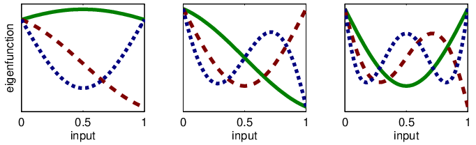
For ordinary kriging,
The value of , the variance of , is given by
which implies different points in the space have differing variances. Typically points in the middle of , which have significant amounts of integrated covariance, have smaller variance under this model. To illustrate take and let , where is a lengthscale parameter, then
where is the cumulative probability distribution for a Gaussian random variable. This property carries over to higher dimensional functions. For example, if the input space is and the correlation function is the product of one-dimensional Gaussian covariance functions, then the point with the smallest variance of is be the center of the space, .
There are implications, using this orthogonal Gaussian process model, in the design of computer experiments. The mean squared prediction error over the space is
The idea is to choose a design such that that minimizes some aspect of the MSPE, such as its expected value (Sacks et al. (1989)) . Using the orthogonal Gaussian process model, we have that
where and are the portions of the predictor that correspond to the mean and random field elements. Under the conditions of Theorem 1,
Thus, choosing designed experiments under the orthogonal Gaussian process models may be more transparent compared to other universal kriging models. When using orthogonal Gaussian process models, separate criteria can be used to evaluate the performance of designs for the mean and random field portions of the response. A thorough investigation of experimental designs under the orthogonal Gaussian process model is outside the scope of this paper.
3 Fast computation of the covariance function
After obtaining a predictor, it is evaluated numerous times for optimization and uncertainty quantification. If the integrals in (4) need to be evaluated for each new prediction, the predictor becomes expensive to evaluate and the advantages it possess in terms of estimation and interpretability significantly diminish. It is important to find ways to evaluate the integrals quickly.
For notational simplicity in this section, each vector has components labeled and subscripts give dimensional indexing. Assume the input is located in the Cartesian product of intervals, . Let the function be a separable covariance function, where the are positive definite covariance functions on and let = where the are mappings from to a -dimensional vector and indicates the Hadamard product.
Here, the high-dimensional integrals can be reduced to single dimensional integrals, i.e.
Now consider that each of the basis functions in are products of one-dimensional linear functions. Let th element of be where is subset of . For example, if is the empty set, then the th element of is , the constant function and if , then the th element of is . These basis functions are typically chosen based on effect heredity principle (Wu and Hamada (2009)) , under which is included only if at least one of its subsets defines another basis function (weak heredity) or only if all of its subsets define other basis functions (strong heredity).
Suppose the sets , , define , and consider the functions
the mean and linear effects, respectively. The th element of is If we take
| and |
is the integrated mean effect, is the integrated linear effect, and is the integrated linear-linear effect. The th element of the matrix is then
Despite the friendly structure, the results still require the evaluation of an integral to find the covariance. There are a few covariance functions for which these integrals have closed forms. Thus if
| (7) |
and , then
Here is because the variables are scaled in , making a diagonal matrix, which further simplifies the computation of the covariance function as
| (8) |
Similar results can be found for the exponential and the Matèrn covariance functions for certain values of the smoothness parameter. The appendix lists two forms of the covariance corresponding to these cases.
4 Numerical illustrations
Here, we compare the proposed method, universal kriging, and another common method using least squares. In the last method, we set and use kriging on the residual, giving
The third method is included because it does not have an obvious identifiability problem and is thus a reasonable comparison. It produces the same results for the mean function as restricted spatial regression (Hodges and Reich (2010)) .
4.1 One-dimensional input
Let and . As is increased, the output increases, thus we try a trend function . We use three covariance functions to illustrate the ideas (the Gaussian, exponential and the Matérn): , and These are covariances for which we have derived explicit statements for the covariance. The lengthscale parameter was fixed at a reasonable value for illustrative purposes here. It will be estimated in the next section.

We chose two observation schemes: and . Figure 3 shows the estimated mean function for all methods under the two observation schemes when the correlation function is Gaussian. In the first scheme, the orthogonal Gaussian process method clearly outperforms universal kriging in estimation of the trend; in the second, more friendly observation scheme, universal kriging still does a poor job of estimating the trend due to identifiability issues.
Prediction performance is shown in Table 1. The Gaussian has the best predictive power here, but under all choices of covariance functions, the difference between the methods is small. The major gains of the proposed approach are seen in the estimated parameters, where the mean function parameters are most stably estimated using it when the observation schemes are changed (see the last column of Table 1).
| Observation Scheme #1 | Observation Scheme#2 | |||||||
| RMSPE | RMSPE | |||||||
| LS, Gaussian | ||||||||
| OGP, Gaussian | ||||||||
| UK, Gaussian | ||||||||
| OGP, Matérn | ||||||||
| UK, Matérn | ||||||||
| OGP, Exponential | ||||||||
| UK, Exponential | ||||||||
4.2 Borehole function
Consider the borehole function (Worley (1987)) , given by
The space is the rectangular region . We scaled it to use (8).
We took the mean function . We generated a random Latin hypercube design times for sample sizes of , , and . Because of the function’s smoothness, we adopted the Gaussian covariance function (7). We did not a priori chose ; we selected it as the maximum likelihood estimate,
with replacing for the orthogonal Gaussian process method and the least squares estimate instead of for the final method. The above optimization problem was restricted to .
The results of the simulations are summarized in the supplementary material. The mean square prediction error is essentially the same under each approach. Figure 4 shows boxplots across 50 replicates for the first two ’s. Using universal kriging, has only a small reduction in standard deviation as the sample size is increased to , indicating a lack of convergence. When , the standard deviation of the estimate of using orthogonal Gaussian processes is ten times smaller than the estimate using universal kriging. The results using universal kriging are significantly worse for , which appears to be centered at different values depending on the sample size. While the least squares estimates appear to be converging to reasonable values, convergence is slow relative to the orthogonal Gaussian process model. From a modeling standpoint, this may be because the least squares estimates do not incorporate the smoothness of the response (Tuo et al. (2015)) .

Figure 5 contains an illustration when . To show the high-dimensional functions, we plot the functions while integrating all but the th variable, . Here, a user using to understand the borehole function may reach incorrect conclusions by choosing universal kriging or least squares over the orthogonal Gaussian process method. This can have important implications in identifying the causes of discrepancy in model calibration problems (Joseph and Yan (2015)) .

5 Application in multi-fidelity simulations
A frequently encountered problem in computer experiment analysis is the fusion of multi-fidelity simulations ( Kennedy and O’Hagan (2000) , Tuo et al. (2014) ). For example, consider simulations with only two levels of accuracy ( Qian et al. (2006) , Qian and Wu (2008) ). The low-accuracy simulations are cheaper, whereas the high-accuracy simulations are expensive and the aim is to predict the output using fewer expensive simulations. Following Kennedy and O’Hagan (2000), let be , where is the low-accuracy response and is the high-accuracy response. The model is thus where is a Gaussian process. For simplicity, we assume to be available in analytical form. Since and have particular meaning in this context, it becomes imperative that they be estimated well, and the universal kriging approach (which is implied by Kennedy and O’Hagan (2000)) can give misleading results.
To illustrate these ideas, consider two examples presented in Ba et al. (2013) and Qian et al. (2006). In the first, two responses exist and are analyzed separately. Since the low-accuracy response used by Qian et al. (2006) was unavailable to us, the linear low-accuracy response was used instead, with a vector of the design variables as ordered in Table 2 of Qian et al. (2006). The between their data and this linear model was over . The covariance was a Matèrn covariance covariance function with the lengthscale parameters equal to the twice the ranges of each input. For the computation of and , numerical quadrature was used to solve to sufficient accuracy. The integration results from Section 3 can be used to simplify the expression for and in the second example because the model is linear. There is no ability to compute RMSPE because the high-accuracy response can only be evaluated a finite number of times due to time and resource constraints, as detailed in the respective papers.
Table 2 shows the different conclusions one arrives at when using the estimation methods. In the Ba et al. (2013) example, universal kriging produced significantly different parameters from the other methods. The universal kriging estimates of the location parameters are very large in both examples. For the second response, the universal kriging estimate of is negative, indicating that the low-accuracy model does not correspond to the high-accuracy response. If universal kriging’s estimated parameters were directly used to draw conclusions, a user might wish go back and adjust the low-accuracy responses. The orthogonal approach tells a different story, with close to and close to for both responses. Thus the parameters from the orthogonal approach indicate that the low-accuracy responses are good representations of the high-accuracy responses. For the Qian et al. (2006) example, all approaches similarly estimate the scale parameter, but the sign of the estimated location parameter is flipped with the orthogonal Gaussian process method. Moreover, both the orthogonal approach and the universal kriging approach place the scale parameter very close to compared to the least squares approach. Thus in both datasets, information gleaned from the estimated parameters varies based the chosen estimation method. Based on the simulations in Sections 4.1 and 4.2, it would appear that the orthogonal Gaussian process estimates have some advantages over the other two approaches.
| Ba et al. (2013) | Qian et al. (2006) | |||||
| response 1 | response 2 | |||||
| LS | 1.43 | 1.06 | 0.33 | 0.99 | -0.35 | 1.03 |
| OGP | 0.43 | 1.08 | 1.43 | 0.99 | 0.16 | 1.00 |
| UK | -34.12 | 1.29 | 88.03 | -1.67 | -0.66 | 1.00 |
6 Conclusions and discussion
The accurate estimation of the mean function is important in many applications involving computer model calibration, global sensitivity analysis, and spatial random effects modeling. The identifiability problem can be avoided by making the mean function orthogonal to the random field, and in this article, we have proposed a Gaussian process model that has this property. This is achieved by modifying a given covariance function to incorporate the orthogonality condition. While these covariances are defined by integrals, some versions of the covariance functions can be quickly evaluated. This paper has focused on the modeling aspect of the problem and numerical examples show quite promising results for estimation.
7 Supplementary Materials
The online Supplementary Materials contains additional information for section 4.2 in the paper.
Acknowledgements
This research is supported by a U.S. National Science Foundation grant CMMI-1266025 and a U.S. Department of Energy Advanced Scientific Computing Research Award ERKJ259.
Appendix: Proof of Lemma 1
Since is continuous, we can choose a measurable version of the process such that
(Marcus and Shepp (1972)) . Then
by the assumption of being bounded. Thus we can appropriately switch integral and expectation signs and note that the covariance matrix of is
where is the matrix Since is positive definite, this matrix is positive semidefinite and is positive semidefinite. As , is positive semidefinite for all .
Appendix: Proof of Theorem 1
We have that and then
Consider the th element of , , where is the th value of . We show this has mean and variance , thus is with probability one.
Since is continuous, we can choose a measurable version of the process and then
As in Lemma 1, we can switch the expectation and integral to get
Expanding the variance term yields
Appendix: Other versions of the orthogonal covariance
This section details other explicit forms of the covariance that mirror the statement of (8). Let each vector have components labeled . We use subscripts for all dimensional indexing in this section. Assume the input is located in the Cartesian product of standard intervals, . Let the th element of be where is subset of . Consider the exponential covariance
When it is used, the values of the function and constants in (8) are
The Matèrn covariance, when the smoothness parameter is given by , is
When it is used, the values of the function and constants in (8) are
References
- Ba et al. (2013) Ba, S., Jain, N., Joseph, V. R. and Singh, R. (2013) Integrating analytical models with finite-element models: an application in micromachining. Journal of Quality Technology, 45, 200–213.
- Bursztyn and Steinberg (2006) Bursztyn, D. and Steinberg, D. M. (2006) Comparison of designs for computer experiments. Journal of Statistical Planning and Inference, 136, 1103–1119.
- Cressie and Cassie (1993) Cressie, N. A. and Cassie, N. A. (1993) Statistics for Spatial Data. Wiley New York.
- Currin et al. (1991) Currin, C., Mitchell, T., Morris, M. and Ylvisaker, D. (1991) Bayesian prediction of deterministic functions, with applications to the design and analysis of computer experiments. Journal of the American Statistical Association, 86, 953–963.
- Hanks et al. (2015) Hanks, E. M., Schliep, E. M., Hooten, M. B. and Hoeting, J. A. (2015) Restricted spatial regression in practice: geostatistical models, confounding, and robustness under model misspecification. Environmetrics, 26, 243–254.
- Hodges and Reich (2010) Hodges, J. S. and Reich, B. J. (2010) Adding spatially-correlated errors can mess up the fixed effect you love. The American Statistician, 64, 325–334.
- Hughes and Haran (2013) Hughes, J. and Haran, M. (2013) Dimension reduction and alleviation of confounding for spatial generalized linear mixed models. Journal of the Royal Statistical Society: B, 75, 139–159.
- Joseph and Yan (2015) Joseph, V. R. and Yan, H. (2015) Engineering-driven statistical adjustment and calibration. Technometrics, 57, 257–267.
- Kariya and Kurata (2004) Kariya, T. and Kurata, H. (2004) Generalized Least Squares. John Wiley & Sons.
- Kennedy and O’Hagan (2000) Kennedy, M. C. and O’Hagan, A. (2000) Predicting the output from a complex computer code when fast approximations are available. Biometrika, 87, 1–13.
- Kennedy and O’Hagan (2001) — (2001) Bayesian calibration of computer models. Journal of the Royal Statistical Society: B, 63, 425–464.
- Marcus and Shepp (1972) Marcus, M. B. and Shepp, L. A. (1972) Sample behavior of gaussian processes. In Proceedings of the Sixth Berkeley Symposium on Mathematical Statistics and Probability (eds. L. M. Le Cam, J. Neyman and E. L. Scott), vol. 2, 423–441. Berkeley, Calif.: University of California Press.
- Matheron (1963) Matheron, G. (1963) Principles of geostatistics. Economic Geology, 58, 1246–1266.
- Paciorek (2010) Paciorek, C. J. (2010) The importance of scale for spatial-confounding bias and precision of spatial regression estimators. Statistical Science, 25, 107–125.
- Qian and Wu (2008) Qian, P. Z. G. and Wu, C. F. J. (2008) Bayesian hierarchical modeling for integrating low-accuracy and high-accuracy experiments. Technometrics, 50, 192–204.
- Qian et al. (2006) Qian, Z., Seepersad, C. C., Joseph, V. R., Allen, J. K. and Wu, C. F. J. (2006) Building surrogate models based on detailed and approximate simulations. Journal of Mechanical Design, 128, 668–677.
- Rasmussen and Williams (2006) Rasmussen, C. E. and Williams, C. (2006) Gaussian Processes for Machine Learning. MIT Press.
- Reich et al. (2006) Reich, B. J., Hodges, J. S. and Zadnik, V. (2006) Effects of residual smoothing on the posterior of the fixed effects in disease-mapping models. Biometrics, 62, 1197–1206.
- Rue and Held (2005) Rue, H. and Held, L. (2005) Gaussian Markov Random Fields: Theory and Applications. CRC Press.
- Sacks et al. (1989) Sacks, J., Welch, W. J., Mitchell, T. J. and Wynn, H. P. (1989) Design and analysis of computer experiments. Statistical Science, 4, 409–423.
- Santner et al. (2003) Santner, T. J., Williams, B. J. and Notz, W. (2003) The Design and Analysis of Computer Experiments. Springer.
- Singh et al. (2011) Singh, R. K., Joseph, V. R. and Melkote, S. N. (2011) A statistical approach to the optimization of a laser-assisted micromachining process. The International Journal of Advanced Manufacturing Technology, 53, 221–230.
- Smith (2014) Smith, R. C. (2014) Uncertainty Quantification: Theory, Implementation, and Applications. SIAM.
- Steinberg and Bursztyn (2004) Steinberg, D. M. and Bursztyn, D. (2004) Data analytic tools for understanding random field regression models. Technometrics, 46, 411–420.
- Tuo et al. (2014) Tuo, R., Wu, C. F. J. and Yu, D. (2014) Surrogate modeling of computer experiments with different mesh densities. Technometrics, 56, 372–380.
- Tuo et al. (2015) Tuo, R., Wu, C. J. et al. (2015) Efficient calibration for imperfect computer models. The Annals of Statistics, 43, 2331–2352.
- Worley (1987) Worley, B. A. (1987) Deterministic uncertainty analysis. Tech. Rep. ORN-0628, Oak Ridge National Lab., TN (USA).
- Wu and Hamada (2009) Wu, C. F. J. and Hamada, M. S. (2009) Experiments: Planning, Analysis, and Optimization. John Wiley & Sons, 2 edn.