Introduction to the physics of the total cross-section at LHC
Abstract
This review describes the development of the physics of hadronic cross sections up to recent LHC results and cosmic ray experiments. We present here a comprehensive review - written with a historical perspective - about total cross-sections from medium to the highest energies explored experimentally and studied through a variety of methods and theoretical models for over sixty years. We begin by recalling the analytic properties of the elastic amplitude and the theorems about the asymptotic behavior of the total cross-section. A discussion of how proton-proton cross-sections are extracted from cosmic rays at higher than accelerator energies and help the study of these asymptotic limits, is presented. This is followed by a description of the advent of particle colliders, through which high energies and unmatched experimental precisions have been attained. Thus the measured hadronic elastic and total cross-sections have become crucial instruments to probe the so called soft part of QCD physics, where quarks and gluons are confined, and have led to test and refine Regge behavior and a number of diffractive models. As the c.m. energy increases, the total cross-section also probes the transition into hard scattering describable with perturbative QCD, the so-called mini-jet region. Further tests are provided by cross-section measurements of , and for models based on vector meson dominance, scaling limits of virtual photons at high and the BFKL formalism. Models interpolating from virtual to real photons are also tested.
It seems to us to be a necessary task to explore bit-by-bit the rigorous consequences of analyticity, unitarity and crossing.
Who knows if someday one will not be able to reassemble the pieces of the puzzle. - A. Martin and F. Cheung, based on 1967
A.M. Lectures at Brandeis Summer School and Lectures at SUNY and Stony Brook [1].
pacs
13.85.Lg Total cross sections and 13.85.DzElastic scatteringIntroduction
This review aims at illustrating the development of studies of total hadronic cross-sections in a historical perspective, primarily for hadrons and photons at high energies.
The optical theorem relates a total cross-section linearly to the absorptive part of a forward elastic amplitude. Moreover, at very high energies, as the imaginary part of the forward amplitude dominates the real part, the elastic differential cross-section in the forward direction becomes proportional to the square of the total cross-section. Thus, discussions about total cross-sections become entwined with that of elastic cross-sections. Hence, in this review considerable attention is also paid both to experimental and theoretical aspects of the elastic cross-sections.
As this rather lengthy review discusses many subjects, we provide below a quick overview to help a reader choose sections of the review that may be of particular interest. Serving mostly as a guide through the large material we shall deal with, no references are included in this general introduction, but they are of course available in the individual sections, at the beginning of which we provide a description of contents and a brief guide to the subsections.
In Section 1, kinematics and partial wave expansions are obtained for the elastic amplitude and general principles, such as unitarity, are employed to derive the optical theorem. An introduction to the asymptotic behavior is provided via the Regge formalism, the Pomeranchuk theorem and finite energy sum rules. Through analyticity, Martin-Froissart rigorous upper bounds are established for the total cross-sections. For charged particles, the EM (Coulomb) amplitude is mostly real (and large near the forward direction) and hence measurements of the needed real part of the “strong” forward amplitude (and measurement of the ratio of the real to the imaginary part of the forward scattering amplitude, the so-called parameter) often involve Coulomb interference and soft radiation. We discuss it in some detail and supplement it with a proposal to employ soft radiation as a tool to measure total cross-sections.
In Section 2, we discuss how cosmic radiation is employed as a non-accelerator method to measure total cross-sections and provide valuable information at energies substantially larger than those of earth bound accelerators such as the Large Hadron Collider (LHC). Along with some history of the subject beginning with Heisenberg, a description of the Glauber formalism for nuclei is presented for the extraction of cross-sections from data and corresponding uncertainties in the models are discussed. We follow the historical path which led to the advances in experimental techniques and theoretical methods that continue to provide a unique window towards fundamental physics and astrophysics, at energies otherwise unreachable through accelerators in the foreseeable future. Recent theoretical results about the power law spectra in the cosmic ray energy distribution both for fermions (electrons/positrons) and bosons (Helium and other nuclei) are briefly discussed and shown to agree with high precision data from AMS, Auger and other Collaborations.
Section 3 deals with pre-LHC measurements of , the total and cross-section, such as those made at the CERN Intersecting Storage Rings (ISR), the CERN and the FermiLab Tevatron. These pioneering experiments verified the rise with energy of - suspected from experiments with cosmic rays - and of the slope parameter , which defines the behaviour of the elastic differential cross-section in the forward region, as well as discovered considerable variations in the parameter. The black disk limit and how close we may be to it are also discussed herein.
In Section 4, we provide theoretical scenarios and phenomenology of the elastic amplitude and hadronic cross-sections, that span over 80 years, beginning with the original Molière theory of multiple scattering, followed by Heisenberg’s considerations about the energy behavior of , and culminating in various QCD inspired models. Eikonal and Regge models are discussed along with hadronic matter distribution. We recall the development in QED of the need for soft-photon re-summation to avoid the infra-red (IR) catastrophe, and the semi-classical, but Lorentz covariant, methods for soft radiation subsequently developed. As a corollary, a Regge trajectory for the photon is obtained. These methods are extended to discuss soft QCD radiation and the divergent nature of of strong coupling constant for small transverse momenta . Asymptotic behavior of scattering amplitudes in QCD, the Balitsky, Fadin, Kuraev and Lipatov (BFKL) equation and spontaneously broken gauge theories are discussed along with the Reggeization of the gauge particles therein. Next, eikonal mini-jet models for and their phenomenology are developed. A brief description of the AdS/CFT correspondence for is presented. Also, some details of the phenomenology of by the COMPETE and COMPASS collaborations are provided.
Details of the energy and momentum transfer dependence, the slope, the dip, the real and the imaginary parts of the elastic (and diffractive) amplitude are discussed in Section 5. Early models and their updates such as Durham, Tel Aviv, mini-jet and multi-pomeron models, are presented as required by more refined data. A concise summary of the model results are also provided.
Photon processes are discussed in Section 6 beginning with kinematics of interest for real versus virtual photons and the relevant parton model variables. Sakurai’s vector meson dominance, Gribov’s model and photo-production at HERA is taken up next, along with and processes at LEP and factorization. The transition from real to virtual photon processes is discussed and models such as Haidt’s are presented. The results of the Tel Aviv and mini-jet models with soft gluon resummation are discussed. The Balitsky-Kovchegov (BK) equation and its various applications such as geometrical scaling are considered and directions beyond into Pomeron loops, explored.
Section 7 discusses the layout of the LHC experimental areas as had been planned before its start. Expectations were to produce total cross-section data with accuracy after a 3 year run. It is gratifying to note that forward physics data with accuracy have already been achieved. The highest energy physics results are shown for the total, elastic and inelastic cross-sections at presently reached LHC energies, and TeV, obtained by the TOTEM, ATLAS and CMS groups. Predictions at are indicated.
1 The theoretical framework from unitarity and analyticity
This chapter is devoted to a review of the basic formalism pertaining to elastic scattering and to the well-established theorems on total, elastic and inelastic cross-sections. Here analyticity and unitarity play a crucial role for the scattering of hadrons, protons and mesons, such as pions and kaons, while scattering of their QCD constituents and their contribution to total cross-section dynamics will be introduced when dealing with QCD models.
For this material, there exist both books and reviews, nonetheless we reproduce most of the relevant material to introduce, in a modern language, the necessary notation and put together all the theorems which are important for our present understanding of hadronic physics or for optimal fitting of the existing data. One case at hand is whether the limitations imposed by the Froissart bound are satisfied and another case is the application to very high energy data fitting by Finite Energy Sum Rules (FESR), derived from analyticity and crossing.
We shall discuss the early formalism of the partial wave expansion of the elastic scattering amplitude, needed to understand the Martin-Froissart theorem, and relate it to the Regge pole expansion which played a major role in phenomenological description of inclusive and total cross-sections in the ’60s and ’70s. To accommodate such a description and the rise of , the Pomeron trajectory corresponding to the exchange of a state with the quantum numbers of the vacuum was introduced. Thus, a picture of , with a Regge and a Pomeron exchange, unrelated to the underlying parton dynamics of scattering, was one of the first and still very successful descriptions. Finally, from the partial wave expansion for the amplitude, and through the optical theorem, we shall introduce the eikonal representation of the total cross-section. This representation is at present the major formalism, into which QCD models for the energy behaviour of are embedded. This chapter is divided with section and subsection headings as indicated in the following:
- •
General principles behind relativistic scattering amplitudes in 1.1
- •
Kinematics and analyticity of elastic amplitudes in 1.2
- •
Probability conservation and unitarity in 1.3
- •
The optical theorem and total cross-section in 1.4
- •
Partial wave expansion of elastic amplitudes in 1.5
- •
Regge expansion and asymptotic behaviour of amplitudes in 1.6
- •
Finite energy sum rules and duality for the elastic amplitudes in 1.7
- •
Various derivations of the Martin-Froissart bound in 1.8
- •
The Pomeranchuk theorem in 1.9
- •
1.1 General principles
Strong interactions are presently understood in terms of interactions between quarks and gluons. Quantum chromodynamics (QCD) can give remarkably accurate results within perturbation theory, when dealing with very high energy collisions and their final products in the large momentum transfer processes. However, the bulk of collisions among high energy particles involves low momentum partons which escape the perturbative treatment. For this purpose, we have to resort to some general principles -valid beyond perturbation theory- to establish the necessary formalism and derive some general theorems. Later we shall develop some tools to include QCD phenomena in this general picture.
These general principles were established in the late ’50s and consist of unitarity, analyticity and crossing symmetry. Each of them is related to basic axioms:
- •
unitarity to the conservation of probability in scattering processes;
- •
analyticity to causality and
- •
crossing symmetry to the relativistic nature of the interaction.
These basic principles are also at the foundations of relativistic Quantum Field Theory (QFT) [2].
We shall describe in detail how one obtains the so-called Froissart bound, which imposes limits to the asymptotic behavior of the total cross-section in two particle scattering. This limit was obtained first by Froissart [3] and successively reformulated by Martin [4] and Lukaszuk [5]. The importance of this limit cannot be understimated, as most efforts to describe theoretically the total cross-section behaviour or most fits to present data must contemplate the asymptotic satisfaction of the Froissart bound. For this reason we shall describe how this limit is obtained in several different derivations, pointing out in all cases the common hypothesis, which is always the presence of a finite mass in final state scattering.
The basic quantity to study in particle physics is the probability that a certain set of particles in a given initial state undergo a collision and scatter into a final state .
To this effect, the process is described by the quantity
| (1.1.1) |
where is called the S-matrix (S for scattering) and are the matrix elements. Since the scattering must also include the possibility that nothing occurs, the S-matrix is written in terms of the -matrix, namely
| (1.1.2) |
where the 4-dimensional -function imposes energy-momen–tum conservation on all particle momenta , and, with obvious notation, . The relevant matrix elements define the scattering and are functions of the momenta of the scattering particles, in particular of the various invariants which can be constructed with the momenta. Let us then turn to the kinematics before going further into the dynamics.
1.2 Kinematics of elastic scattering
Let us consider the two body process
| (1.2.1) |
Usually, two different set-ups are most frequently encountered: center of mass collisions, as in most if not all present day accelerator experiments at high energies; and fixed target collisions, as is the case for cosmic ray proton-air collisions or low energy photo-production experiments. It is usual to call Laboratory frame where fixed target collisions take place. However, there is another frequently encountered possibility, namely the kinematic configuration of two collinear particles of different momentum. This situation is found in electron and photon proton collisions at HERA and generally speaking is typical of parton-parton collisions. We shall present in the following the kinematics of all these three different possibilities.
In the c.m. frame of particles and , we write
| (1.2.2) | |||
| (1.2.3) | |||
| (1.2.4) | |||
| (1.2.5) |
which can be described by two independent variables, to be chosen among three relativistic invariants, the so called Mandelstam variables, i.e.
| (1.2.6) | |||
| (1.2.7) | |||
| (1.2.8) |
For general processes, we have
| (1.2.9) |
and thus for elastic scattering, namely
| (1.2.10) |
we have with
| (1.2.11) | |||
| (1.2.12) |
and
| (1.2.13) | |||
| (1.2.14) |
where is the scattering angle in the c.m. frame.
For collisions not taking place in the center of mass, the kinematics reads differently. While and scattering in present day accelerators take place through center of mass collisions, this was not true for early experiments, where typically a proton or antiproton was directed to a fixed hydrogen target, and it is also not true for meson proton scattering, such as , or , where pions, kaons or photons are directed to a fixed hydrogen target. In such cases, for the kinematics in the laboratory frame we get
| (1.2.15) |
so that
| (1.2.16) | |||
| (1.2.17) | |||
| (1.2.18) |
In all the above cases, the proton is at rest in the laboratory. A different case is the one encountered at HERA, where the two beams, photons and protons, collide with different momenta. For real photons of momentum colliding with a proton of energy , one has
| (1.2.19) |
Kinematics is still different for virtual photon scattering and will be described in Sect. 6.
Because of energy momentum conservation and of the condition imposed by Eq. (1.2.9), physical processes can take place only for those values of the variables s, t and u which lie in the so called physical region. Such a region is defined as [2]
| (1.2.20) |
where
| (1.2.21) | |||
| (1.2.22) | |||
| (1.2.23) |
For the equal mass case, this reduces to the condition and the allowed regions are shown in the dashed areas of Fig. 1.1.
1.3 Unitarity and the scattering amplitude
The measurement of the total cross-section is based on two complementary methods: counting the number of collisions and, measuring the very forward scattering probability. The second method is based on a fundamental physical property i.e., the conservation of probability, which is embedded in the unitarity property of the S-matrix, namely
| (1.3.1) |
In terms of the matrix elements, we have
| (1.3.2) |
where runs on all possible intermediate states. This condition ensures the normalization and orthogonality of states in the reaction. In particular, for the case, Eq. 1.3.2 ensures that the sum over all allowed transitions from a given state to any possible final state, is one, namely
| (1.3.3) |
Eq. (1.3.3) is the statement of conservation of probability in the scattering.
We can now proceed to derive the optical theorem, by using Eqs. (1.3.2) and (1.1.2) to obtain
| (1.3.4) |
Because the left hand side of this equation is linear in T, while the right hand side is quadratic, if the T-matrix can be expanded in a small parameter (say a coupling constant), then unitarity ensures that the T-matrix elements are hermitian. In the general case, one uses Eq. (1.3.4) to obtain the optical theorem, namely
| (1.3.5) |
where the amplitude indicates elastic scattering in the forward direction and where the right hand side, a part from a normalization factor, gives the total cross-section for scattering from an initial state into any possible final state, as shown in the following subsection. The reader is warned that different authors use different normalizations for the elastic scattering amplitudes and hence due care must be taken in using various unitarity expressions.
1.4 The optical theorem and the total cross-section
We follow here the definitions and normalizations as in [6]. Let us start with the general definition of total cross-section, by first introducing the probability that a given two particle initial state scatters into all possible final states , namely
| (1.4.1) |
where the sun runs over all final states and all possible quantum numbers of all possible final states. Next we use the S-matrix definition in terms of the T-matrix
| (1.4.2) |
and define the probability of the scattering per unit volume and unit time, by using the conventional way to interpret as the four-dmensional scattering volume VT. Using the language of the laboratory frame, where the initial state consists of a target particle (T) and a projectile (P), a further step is taken by considering the scattering per target particle, dividing by the target particle density , and obtaining the cross-section by further dividing this probability by the flux of incoming particles, . We then have
| (1.4.3) |
The next step is to use Eq. (1.3.5) to relate the total cross-section to the imaginary part of the forward scattering amplitude so as to obtain, in the cm frame,
| (1.4.4) |
where is the center of mass momentum of the incoming particles and the c.m. energy. We then see that the total cross-section can be measured in two different ways, either through the total count of all the final states hitting the detector or through the imaginary part of the forward elastic amplitude. In the next section, we will establish some definitions and properties of the elastic scattering amplitude.
1.5 The elastic scattering amplitude and its partial wave expansion
For two equal-mass particle scattering in the c.m. system, the Mandelstam invariants take a particularly simple form and the physical region for the s-channel is defined as
| (1.5.1) | |||
| (1.5.2) |
Let then the elastic scattering amplitude be expanded in a series of Legendre polynomials
| (1.5.3) |
where the subscript refers to the normalization used by Froissart. Martin’s normalization differs by a factor , namely
| (1.5.4) |
For simplicity, we shall now use . Using elastic unitarity, it is rather simple to obtain some limits on the partial wave amplitudes .
1.6 Asymptotic behaviour and Regge theory
We present here a brief description of the Regge expansion which has been very useful in molding our ideas about the behavior of elastic and total cross-sections as a function of energy. The Regge picture forms the backbone of high energy phenomenology of cross-sections. To illustrate its central theme, let us consider the partial wave expansion of an elastic scattering between two equal mass spinless particles of mass
| (1.6.1) |
where the partial wave amplitude and . This expansion, for physical -channel scattering () certainly converges for . The Regge expansion consists in obtaining a representation valid for large through a continuation from integral values of to continuous (complex) values of via the Sommerfeld-Watson (W-S) transformation. In non-relativistic potential scattering, Regge was able to prove that for a superposition of Yukawa potentials, the amplitude is an analytic function of and its only singularities are poles [the famous Regge poles, )] and that bound states and resonances are simply related to them. The situation in the relativistic case is less clear and technically more involved[7, 8] For integral values of , Eq. (1.6.1) can be inverted to give
| (1.6.2) |
While the above equation permits an analytic continuation of the function to complex values of , it is not suitable for completing the W-S transformation due to the bad asymptotic behavior of for complex [7]. Hence, a technical nicety, the Froissart-Gribov projection, is required. Assume that is polynomially bounded so that that a fixed -dispersion relation (with N subtractions) can be written down in the variable :
| , | (1.6.3) |
where and are the and channel discontinuities of the amplitude. Substituting the above in Eq. (1.6.2), we find that
| (1.6.4) |
obtained upon using the identity
| (1.6.5) |
Since for positive integral values of , , we may rewrite Eq. (1.6.4) as
| (1.6.6) |
where is the smaller of and . To avoid obtaining dangerous factors such as for complex when we analytically continue Eq. (1.6.6), it is useful to define the “signatured” Froissart-Gribov amplitudes
| (1.6.7) |
which can be continued for all , since in this region, the above integrals converge. The positive signature amplitude for even and the negative signature for odd . Thus, the W-S transformation is to be performed on the signatured total amplitudes
| (1.6.8) |
separately. The physical amplitude is then given by the combination
| (1.6.9) |
For each of the amplitudes in Eq. (1.6.8), one first replaces the sum by a contour C which encircles all the integers in the sum
| (1.6.10) |
since the function has poles at all the integers with residue and use has been made of the property that for integers . The next step is to open the contour as in Fig. 1.2

and one finds a large semi-circle in the positive quadrant, a background integral running vertically at and the contributions from any singularities in . We expect Regge poles and perhaps Regge cuts. Ignoring the cuts for the moment, we may write
| (1.6.11) |
where the sum includes all poles with and the corresponding denote their residue. For large (which is synonymous with large for fixed ), and thus, in this limit would be controlled by the Regge pole to the farthest right (called the leading Regge pole). Hence, one arrives at the Regge asymptotic behavior result that
| (1.6.12) |
in the limit for fixed . Of course, had we made the Regge expansion in the channel, we would have obtained the result
| (1.6.13) |
in the limit for fixed. Putting in the proper phases, we obtain for the pole contribution to the amplitude (which dominates the background integral for all Regge poles with ) to be of the form
| . | (1.6.14) |
Using the form -valid for large (i.e. ignoring masses)-
| (1.6.15) |
we have
| (1.6.16) |
If , then the total cross-section would go to a constant value. This is the celebrated Pomeron pole. It has the added virtue that the ratio of the real part to the imaginary part of the forward elastic amplitude would be strictly zero, i.e.
| (1.6.17) |
exhibiting the limiting feature of diffraction scattering. Hence, the early excitement about the Pomeron.
By contrast, were , not only would the relative roles of the real and the imaginary parts be reversed but there would be a genuine spin 1 massless physical particle pole (analogous to the photon) in the elastic amplitude. Since in the hadronic spectrum we have have no massless particles -of any spin- we would conclude that if . Hence, there would be no contribution to the total cross-section from an Regge pole (since it would have a vanishing residue). However, the real part may be finite then.
Experimental data clearly indicate that (i) all total cross-sections increase at high energies and that (ii) the “rho” parameter
| (1.6.18) |
Question then arises as to how to implement these facts phenomenologically in a Regge picture. Some theoretical progress has been made regarding the imaginary part in QCD. In the BFKL Pomeron[9] model, one finds that the Pomeron intercept is slightly greater than 1, i.e., , where , where is the QCD coupling constant and is the number of colours ( for QCD). Thus, would rise with energy. While for small enough , this may work for some energy band, it would eventually be in conflict with the Froissart bound discussed at length in the subsequent sections. The Froissart upper bound only permits a maximum increase .
Powers of logarithms can arise due to the confluence of two (or more) pole singularities. For example, if in the angular momentum plane, there occurs a double pole at , its contribution to the W-S integral would be through a derivative (in evaluated at ) [10]. Asymptotically then, if a simple pole gave , a double pole would give . To saturate the Froissart bound, we need two derivatives in i.e., a third order pole, with of course . On the other hand, the more general case, i.e., generation of a fractal power such as
| (1.6.19) |
(as found in a phenomenologically successful model for total cross-section to be discussed later in 4.9.4 of this review) would require a confluence of an indefinite number of pole trajectories all converging at . We remark here in passing that, near a threshold, due to unitarity, a confluence of an infinite number of trajectories (the “threshold poles”) does occur and it has been well studied [10]. It is an open problem to deduce what happens in the vacuum channel of QCD with (almost massless) quarks and gluons. This problem is particularly difficult in QCD because it can only be answered satisfactorily after unitarity is imposed -a daunting task indeed.
The spectrum of mesonic masses leads one to conclude that there are four almost-degenerate Regge trajectories with intercepts close to [8] Hence, in a total cross-section for the scattering of particle with , these terms provide the next to the leading contribution (about half a unit lower than the Pomeron) of the form with the sum running over the , , and Regge trajectories. This nomenclature recalls the lowest spin resonance associated with a given Regge trajectory. As discussed in the FESR and duality section, the approximate degeneracy is deduced from the absence of resonances in “exotic” channels.
Thus, a phenomenological parametrization based on the Regge picure for the high energy total cross-section of particles and may be formulated as [11]
| (1.6.20) |
where the constants , , and are the respective coefficients of the “Pomeron”, an overall constant and the various Regge terms for the scattering process on . The constant obeys the condition () and .
Regarding the asymptotic behavior of the parameter, defined in Eq.(1.6.18), let us use the generic fractal amplitude as given in Eq.(1.6.19)
| (1.6.21) |
where is a real constant and we have employed the phase rule for crossing-even amplitudes[12]. This would give for the asymptotic form for
| (1.6.22) |
This generalizes for arbtrary a rigorous result[13], valid for an amplitude saturating the Froissart bound (here achieved for ).
While it may be difficult to distinguish between a total cross-section increasing as () or [] [or some power in-between for ], it may be easier to use experimental measurements of and employ Eq.(1.6.22) to decipher the value of , since depends on () linearly. In any event, one has two consistency conditions provided by Eqs.(1.6.20) and (1.6.22) for the parameter .
In the next section, we discuss an important off-shoot from the Regge expansion which goes under the names of finite energy sum rules and duality.
1.7 Constraints from FESR and Duality for the total cross-sections
Analyticity in the complex (energy) plane for a function (say a form factor or an elastic scattering amplitude) quite generally implies that its values in the “low” and “high” parts of the complex plane must be intricately related. This obvious fact has been used successfully to relate integrals over the low energy parts of amplitudes to those over their asymptotic high energy (Regge) parts.
To illustrate what is involved, consider the simplest but physically quite important example of the charge form-factor of the proton normalized as . Under the usual hypothesis that for space-like values , the function is real and that it has a right hand cut beginning at the physical charged particle-antiparticle thresholds, , we may write a dispersion relation
| (1.7.1) |
Let us use the extra (experimental) information that for large (space-like) , . Then, Eq.(1.7.1) gives us a sum rule
| (1.7.2) |
which provides a relationship between the integrals over the low and high energy parts of (the imaginary parts) of the form factor. Since also, the neutron charge form facor goes to zero for large , we would obtain an expression analogous to Eq.(1.7.2) also for the neutron except that the right hand side would be zero. In vector meson dominance (VMD) models, the couplings of the , and the to the nucleons get constrained accordingly.
Actually experimental data regarding form factors are much more stringent: it appears that the fall off of the proton form factor is of the “dipole” type. For purposes of illustration, let us assume that as . Then, we can derive a “superconvergence” relation
| (1.7.3) |
Eq.(1.7.3) tells us that must change sign at least once. To meet this exigency then, a generalized vector meson (GVMD) model with other vector mesons etc. with their couplings (of reversed signs) to the nucleons have to be introduced. It is not our purpose here to advocate GVMD models but to illustrate very simply that dispersion relations with some knowledge -be it experimental or theoretical- about the behaviour of an amplitude at some value, allows us to put constraints at other values. 11 1 Sergio Fubini, the discoverer of superconvergence relations, made an analogy between the knowledge of an amplitude locally and some knowledge about the amplitude through sum rules (e.g., superconvergence integrals) to that between Coulomb’s law giving the local value of a field and Gauss’ law providing an integrated statement about the field.
Let us now turn to a specific case that of the elastic meson-baryon amplitudes, with an eye towards their later applications to photon-nucleon total cross sections. For fixed , in order to exploit the crossing symmetry between the and the channels, one defines the variable[8]
| (1.7.4) |
so that denotes the energy of the meson in the rest frame of the baryon and denotes the mass of the baryon. For a crossing-odd scattering amplitude[8] , we may write a fixed- dispersion relation
| (1.7.5) |
Let us assume generic asymptotic Regge terms of the form
| (1.7.6) |
Using arguments previously given, if all the , we would obtain a superconvergence relation
| (1.7.7) |
Instead, we can subtract the contributions from all to obtain a superconvergence relation of the form
| (1.7.8) |
Since asymptotically -by construction- the integrand in Eq.(1.7.8) goes to zero, we may replace the upper limit of the integration to be and include the left over Regge terms with , and find
Doing the integral, we have the finite energy sum rule (FESR)
| (1.7.10) |
Also. higher moment sum rules may be written. For even integer , we have
| (1.7.11) |
FESR can also be constructed for crossing even amplitudes and we shall return to them later.
As emphasized in [8], the relative importance of successive terms in a FESR is the same as in the usual Regge expansion: if a secondary pole is unimportant at a high energy above then this term would be unimportant to exactly the same instant in the sum rule. For elastic scattering in the -channel iso-spin , FESR have been exploited with much success to obtain information about the and the trajectories [14]. Different variants of the idea have been used, see for example [15]
In FESR, the scattering amplitude is multiplied by an integral power of the laboratory energy. This was generalized to continuous moment sum rules(CMSR) [16]. In contrast to FESR, in CMSR, the multiplicative energy factor is non-integral. However, CMSR turn out to be simply a superposition of FESR, if the real part of the amplitude is calculated using dispersion relations [17]. For a review of the applications of these ideas to specific processes, see [18].
An interesting fall out from FESR was the concept of duality[19] which in its final form may be phrased as follows. Consider a generic amplitude and decompose its imaginary part (in the -channel) in terms of the -channel resonances and a smooth background. Then, the assertion is that “direct”() channel resonances are “dual” to the crossed () channel Regge trajectories and the Pomeron term(s) is(are) dual to the background. Explicitly, it means that in Eq.(1.7.11) the integral over the left hand side would contain contributions from (and ) channel (baryonic)resonances whereas the right hand side would contain contributions from mesonic Regge trajectories.
Let us give a practical example of FESR for total cross-section. Suppose experimental data are available for a certain total cross-section within a given energy range. Optical theorem then allows us to convert this into a knowledge about the imaginary part of the forward elastic amplitude in the same energy range. Integrals of this amplitude over the available energy range must match a similar integral for a model describing the same asymptotic amplitude (ergo the asymtotic total cross-section). Thus, unknown parameters in the model, usually Regge residues and intercepts, can be fixed.
For the phenomenolgy of high energy and total cross-sections of interest at the Tevatron and LHC, one forms combinations of the sum and difference of the two cross-sections, thus focusing attention on crossing-even and crossing-odd forward amplitudes. For the odd amplitude , the procedure described above is applicable. For the even amplitude , one constructs an odd amplitude , to which the above arguments again apply. We shall discuss how it works in practice when we discuss models for total cross-sections.
1.8 The Froissart-Martin bound
We shall now derive the Froissart bound following three slightly different methods, the original one by Froissart [3], the one by Martin in [4] and [1], and Gribov’s derivation in [20]. These different derivations expose the different assumptions underlying them.
1.8.1 Froissart’s derivation of the asymptotic behaviour of the scattering amplitude
In [3], the bound on the total cross-section is given an intuitive explanation. It must be noted (in hindsight) that this intuitive explanation relies upon the existence of confinement. Indeed, the whole description applies not to parton scatterings but to hadronic scattering. Let us go through Froissart’s intuitive explanation. Let the two particles (hadrons) see each other at large distances through a Yukawa-type potential, namely , where is some momentum cut-off. Let be the impact parameter, then the total interaction seen by a particle for large is proportional to . When is very small, there will be practically no interaction, while, when is close to , there will be maximal probability for the interaction. For such values of , one then can write for the cross-section . If is a function of energy and we assume that it can grow with energy at most like a power of , then one immediately obtains that the large energy behaviour of the total cross-section is bound by . What is remains undefined for the time being, except that it has dimensions of a mass.
Following this heuristic argument, Froissart’s paper proceeds to the actual derivation of the bound. The derivation is based on the validity of the Mandelstam representation and the optical theorem. From the validity of the Mandelstam representation for the scattering amplitude and the convergence of the partial wave expansion, he derives an upper limit on each partial wave, which depends on the value of angular momentum, after which the partial wave amplitudes become negligible. All the are then put equal to their maximum value and, then, in the forward direction, one has
| (1.8.1) |
The value of is determined as being such that for
| (1.8.2) |
where is the minimum number of subtractions needed for the validity of the Mandelstam fixed- dispersion relations and behaves at most like a polynomial in , q being the c.m.momentum. Eq. (1.8.2) leads to
| (1.8.3) |
and from this through the optical theorem to the bound
| (1.8.4) |
1.8.2 André Martin’s derivation
Martin’s derivation does not require the existence of the Mandelstam representation and is thus more general. Also, it provides an estimate of the constant pre factor to the maximum square of the logarthimic growth. We shall write ignoring all particle masses except when necessary and use his normalization of the elastic amplitude.
| (1.8.5) |
wherein
| (1.8.6) |
is the inelasticity and is the real part of the phase shift and
| (1.8.7) |
denotes the -channel absorptive part of the elastic amplitude. This partial wave series should converge upto .
For the Froissart bound, Martin uses the majorization scheme
| (1.8.8) | |||
| (1.8.9) | |||
| (1.8.10) |
Few remarks:
- •
(i) The first statement, Eq.(1.8.8), assumes that even for large , the partial wave amplitude is elastic and a maximum i.e., and . This is a gross overestimate since we expect that at large , , so realistically we should take and not for low . This then would get the heuristic result Martin obtains towards the end of a recent paper [21] improving the total cross-section bound by a factor .
- •
(ii) Let us also note that Eq.(1.8.8) assumes that the partial wave amplitudes have a sharp cutoff, i.e., its value is exactly for all up to , then brusquely it drops to for and then identically to for all higher . Clearly, this is a very unphysical assumption for a partial wave amplitude and can not be true in any theory which enjoys analyticity in the variable .
- •
(iii) The more reasonable behavior for large , through the convergence of the partial expansion in the Lehmann ellipse leads to times a very smooth function of and . [Eq.(3.4) et sec in Martin’s book [1]]. This is also the discussed in [11] in the context of our BN (Bloch and Nordsieck) inspired model discussed later in 4.9.4, and is the minimum realistic dropoff. However, in obtaining the upper bound, Martin assumes it is identically zero beyond a certain which is certainly true but again unrealistic.
Now to a derivation of the upper bound. Clearly from Eq.(1.8.7) and Eq.(1.8.8), we have that
| (1.8.11) |
To prove the last identity in Eq.(1.8.11), use the recursion identity and then write the sum to be performed in the opposite order (beginning from the end)
| (1.8.12) |
All terms cancel, leaving only two terms
| (1.8.13) |
For large , using Eq.(1.8.7) and Eq.(1.8.13), we have
| (1.8.14) |
Use the Laplace integral for the Legendre function to bound the right hand side:
| (1.8.15) |
so that we can write for the derivative in a useful form
Since , we can bound the above
| (1.8.17) |
Using the mean value theorem, we can impose the bound
| (1.8.18) |
for any . Since and ,
| (1.8.19) |
and hence using Eq.(1.8.14), we have
Taking logarithms of both sides we have
We need only two subtractions in and so . Using it in the above, we arrive finally to the maximum value allowed to
| (1.8.22) |
Now the Froissart bound for the total cross-section follows from
| (1.8.23) |
Letting and , we have the Froissart-Martin result
| (1.8.24) |
All of this can be duplicated in the eikonal scheme and of course much more simply as shown below.
1.8.3 Eikonal Picture derivation
In the limit of large and fixed , the eikonal picture emerges under the hypothesis of identifying the impact parameter formally as , so that
| (1.8.25) |
where is the Bessel function of the “imaginary argument”. With this identification, Eq.(1.8.7) reads
| (1.8.26) |
where the “b-wave amplitude” reads
| (1.8.27) |
We may now impose a similar majorization scheme as before
| (1.8.28) |
whence
| (1.8.29) |
The last integral can be done. Changing variables , we have
| (1.8.30) |
For large ,
| (1.8.31) |
so that, for large
| (1.8.32) |
upon which by taking the logarthims of both sides, and remembering that , we obtain from
| (1.8.33) |
that
| (1.8.34) |
and thus that
| (1.8.35) |
upon imposing .
1.8.4 Gribov’s derivation
What follows is almost verbatim from Sec. (1.4) of [20]. To show that asymptotically
| (1.8.36) |
Gribov proceeds as follows. His notation differs slightly from the one in the previous section. Defining
| (1.8.37) |
with the partial wave amplitudes defined as
| (1.8.38) |
[With respect to Martin, the difference is a factor of ].
Using the fact that the singularity of closest to the physical region of the s-channel is situated at , one tries to estimate at large s. At large , the partial wave amplitude must fall exponentially in order to ensure convergence for . This is a consequence of
| (1.8.39) |
To ensure convergence for , the partial wave amplitudes must then decrease as
| (1.8.40) |
Now, in the limit , , hence and one can write
| (1.8.41) |
where . The function may be a slowly varying (non-exponential) function of .
To establish the Froissart bound, Gribov now assumes that the scattering amplitude grows no faster than a power of , in the vicinity of the pole in the t channel. This condition is analogous to the one about subtraction in Martin’s derivation, just before Eq.(1.8.22). If , one can then see that this also valid for . Let us see how.
| (1.8.42) |
Since all the are positive due to the unitarity condition as well as the for , it must also be true for each term on the sum, namely
| (1.8.43) |
and for it will also be
| (1.8.44) |
and finally we have
| (1.8.45) |
With the bound on , we can now derive the bound on the imaginary part of the forward scattering amplitude and hence on the total cross-section.
| (1.8.46) | |||
| (1.8.47) |
where one has divided the sum into a term where the partial waves are large and for which the partial waves take the maximum value allowed by unitarity, and one which contains all the higher partial waves. To estimate the value of L after which the partial waves are small, consider that they will become less than 1 when
| (1.8.48) |
Now using
| (1.8.49) |
we immediately obtain
| (1.8.50) |
The question arises as to how large are the neglected terms. We can estimate them by using and then sum the second series as
| (1.8.51) |
These terms are at most of order and are subdominant.
Now, using the optical theorem, one obtains the bound
| (1.8.52) |
Thus this demonstration uses
- •
position of the t-channel singularity closest to the s-channel physical region, at
- •
convergence of the partial wave series for (and at most up to the singularity)
- •
large -behaviour of the Legendre polynomials for
- •
that the amplitude does not grow with faster than a fixed power
- •
unitarity condition to ensure that is positive.
1.9 The Pomeranchuk theorem
Here again we follow Gribov. The Pomeranchuk theorem [22] says that, if total hadronic cross-sections go to a constant at very high energy, then asymptotically particle-particle or particle-antiparticle total cross-sections should be equal. It was derived using the property of crossing symmetry of the elastic scattering amplitude.
We know, since the early ’70s, that total cross-section grow with energy [23], and therefore the Pomeranchuk theorem could be considered obsolete. However, there are two reasons to discuss it, one of them being that our understanding of high energy particle collisions if dominated by gluon-gluon scattering in QCD framework, would give the same result as the Pomeranchuk theorem, as discussed later in this section. On the other hand, since the total cross-section is not a constant at high energy, there is space for the existence of the called odderon, whose exchange may be relevant at very high energies. We shall discuss more about this point in later sections.
The Pomeranchuk theorem is derived very simply. First of all, let us move from the discrete representation of the scattering amplitude in angular momentum to the impact parameter space. To do this, one notices that for the total cross-section not to decrease at very high energy, one needs contributions from higher and higher partial waves. At high energy, and in the forward direction, the main contribution to the total cross-section comes from higher partial waves. For large then we can use the asymptotic expression for the Legendre polynomials,
| (1.9.1) |
We can then substitute the sum over the partial waves with an integral and introduce the impact parameter variable . Then the partial wave expansion becomes
| (1.9.2) |
To obtain a constant total cross-section, assume the integral to be dominated by values of the impact parameter whose distribution is independent of the energy : in such a case, the and dependences can be factorized. One puts , to obtain
| (1.9.3) |
Assuming the further possibility that has no residual -dependence, from the optical theorem there follows the constant high energy behaviour of the total cross-section. To summarize, constant total cross-sections can be seen to arise if one can factorize the and dependence in the scattering amplitude, and if the dominant partial wave amplitudes also become constant at very high energy. Both assumptions are not necessarily satisfied. These two assumptions however allow demonstration of the Pomeranchuk theorem, when we use crossing symmetry to relate two processes, in which one particle in the initial state is substituted with an antiparticle from the final state. This amounts to relating the analyticity properties in the -channel to those in the -channel. The argument goes as follows.
Let us consider the two processes
| (1.9.4) | |||
| (1.9.5) |
and let be the amplitude which describes the first of the above processes. The s-channel physical region for process is shown in Fig. 1.3, i.e.

with the usual right-hand cut starting at and the left-hand cut starting at . It is convenient to assume that the amplitude for corresponds to the value above the right-hand cut, namely, to be given by , whereas the crossed process corresponds to exchange with . For the crossed process, the physical region corresponds to , and therefore the physical region for this process, in the channel is obtained by approaching the real axis, on the left hand side, from below, as indicated in Fig. 1.3. Because the amplitude is real for , its value at the edge of the cuts complex conjugates, namely
| (1.9.6) |
but the amplitude at the left-hand side is for process , whereas the one at the right hand side is the amplitude for and one then can write
| (1.9.7) |
Now apply the above result to the elastic amplitude for and consider the imaginary part of the forward amplitude. If the -dependence is of the simple type which leads to constant total cross-section, namely at large s, then optical theorem gives
| (1.9.8) |
For more complicated and -dependences in the amplitude, i.e. those that do not imply constant total cross-sections, Eq. (1.9.8) can still be obtained in some simple cases such as . However, the derivation then needs the additional hypothesis that the real part of the amplitude does not exceed asymptotically the imaginary part, a hypothesis de facto supported by experimental data.
1.10 Determination of the parameter through Coulomb Interference and soft radiation
Here we discuss how near the forward direction, the real part of the hadronic amplitudes is determined through its interference with the Coulomb amplitude. We highlight some of the subtelties associated with the procedure. Also, a proposal is presented for obtaining information about the behavior of the purely nuclear amplitude through the measurement of the soft radiation spectrum in a quiet event, i.e., unaccompanied by any other visible particle.
1.10.1 Coulomb interference
At high energies, the -parameter, which denotes the ratio of the real to the imaginary part of the forward (complex) nuclear scattering amplitude
| (1.10.1) |
is rather small (about ). Since, the total (nuclear) cross-section depends only on and through the optical theorem, the elastic differential cross-section in the forward direction depends on quadratically
| (1.10.2) |
it is difficult to measure accurately and in any event such a measurement would not determine the sign of the real part of the nuclear amplitude.
Fortunately, when we augment the nuclear with the Coulomb amplitude (due to one-photon exchange, in the lowest order), the interference between the Coulomb and the real part of the nuclear amplitude (for small ) allows us to determine both the sign and the value of . The Rutherford singularity () renders the Coulomb amplitude sufficiently large to become competitive with the nuclear term, for small . On the other hand, away from very small angles, the Coulomb term dies out and one can safely revert to the purely nuclear amplitude. However, to obtain numerically accurate information about , some care is required to obtain the correct Coulomb phase for the nuclear problem.
To see what is involved, let us consider first Coulomb scattering in non-relativistic potential scattering. The classical Rutherford amplitude (or, the Born approximation, quantum mechanically), with a Coulomb potential, for the scattering of two charges () and (), is given by
| (1.10.3) |
where denotes the reduced mass, and is the fine structure constant. But, the exact (quantum-mechanical) Coulomb scattering amplitude has an oscillating phase multiplying the above. This phase is given by[24]
| (1.10.4) |
where denotes the relative velocity and the presence of reminds us of the quantum nature of this phase The physical reason for this phase is that the Coulomb potential is infinite range and however far, a charged particle is never quite free and hence is never quite a plane wave. For or scattering, in the relativistic limit () and for small angles, Eq.(3.2.10) reduces to
| (1.10.5) |
Eq.(3.2.11) is exactly the small-angle limit of the relativistic Coulomb phase obtained by Solov’ev[25]. On the other hand, this result was in conflict with an earlier potential theory calculation by Bethe[26] employing a finite range () nuclear potential in conjunction with the Coulomb potential. According to Bethe, the effective Coulomb phase reads
| (1.10.6) |
This discrepancy was clarified by West and Yennie[27]. These authors computed the effective Coulomb phase through the absorptive part of the interference between the nuclear and the Coulomb amplitude. They found -again in the small angle, high energy limit-
| (1.10.7) |
If one ignores the dependence of the nuclear amplitude, the integral term above is zero and one obtains Solov’ev’s result. On the other hand, a result similar to that of Bethe is reproduced, if one assumes the customary fall-off for the nuclear vertex and a dipole form factor for the EM vertex. Explicitly, if we choose
| (1.10.8) |
we find
| (1.10.9) |
where is the Euler-Mascheroni constant. This expression for the effective Coulomb phase agrees with Block[28], upto terms proportional to (), which are quite small near the forward direction. Hence, Eq.(1.10.9) is sufficiently accurate for determining through interference at LHC energies and beyond.
Block has defined a practically useful parameter for which the interference term is a maximum: . For the maximum LHC energy of , . Putting it all together, the Coulomb corrected, differential cross-section for or reads[28]
| (1.10.10) | |||||
where for the magnetic form factor, one may employ , with .
One other aspect of the EM radiative corrections needs to be investigated. So far, we have not considered real soft-photon emissions in the scattering process. As is well known, contributions due to an infinite number of soft photons can be summed via the Bloch-Nordsieck theorem. If denotes the differential cross-section without the emitted soft-photons, the inclusion of soft radiation introduces a parameter which is the external energy resolution . A compact expression for the corrected cross-section can be written as follows[29]
| (1.10.11) |
where the radiative factor combines the various combinations of the momenta of the charged emitting particles in our equal mass elastic case
| (1.10.12) |
where
| (1.10.13) |
In the high energy limit, and , so that the sum vanishes, leaving us with . For small angle scattering of interest here, we have the correction from real photon emission of the form
| (1.10.14) |
where
| (1.10.15) |
which is rather small and vanishes as . The physical reason is that the amount of radiation is small for low velocities. For the CM elastic amplitude, the energy loss due to real soft bremmstrahlung is estimated by the lack of collinearity in the outgoing particles. Thus, ). Even for , the real radiative correction is extremely small and thus can be ignored.
1.10.2 Soft photon radiation as a possible tool for measurements of the total cross-section
Through the above expressions, we may compute the differential probability for a single soft photon produced in association with the near forward elastic process. That is, the differential cross-section for the process , for small and small is given by
| (1.10.16) |
where denotes the nucleon mass.
To obtain a leading order of magnitude estimate, let us insert only the nuclear amplitude in Eq.(1.10.16) and integrate over all :
| (1.10.17) |
Putting in nominal values for the LHC, and for the diffractive width , we estimate
| (1.10.18) |
This would lead us to a comfortable soft photon production rate [associated with elastic scattering]
| (1.10.19) |
where is the machine luminosity. Thus, observation of only soft photons accompanied by no other visible particles (an otherwise quiet event) would be very useful in determining some crucial nuclear high amplitude parameters. Transcending the specific model estimates, what the soft radiation spectrum really measures is the mean value of associated with the elastic cross section .
A simple variant of the procedure outlined above of obtaining information about the background process through the spectrum of a single photon in an otherwise quiet event was utilized earlier at LEP. One way adopted to measure the number of neutrinos into which the could decay consisted in measuring the rate for the process
| (1.10.20) |
Thus, measuring the initial state photon radiation, allowed one to deduce the correct branching ratio of into all neutrino-antineutrino pairs, which obviously escaped experimental detection. On the other hand, at LHC, if indeed a single soft photon spectrum in a quiet event - up to some very small angle - can be measured, one can be reasonably be sure that two protons (to conserve baryon number) must have been produced which escape within the very small angular cone on either side of the beam. Relaxing the angular aperture might allow one to learn something about single diffraction cross section as well. We shall not pursue this interesting topic here any further.
2 Non-accelerator experiments
In this section, we discuss the measurement of proton-proton scattering as performed through cosmic ray experiments, the results and their interpretation.
Until the advent of particle accelerators in the mid-1950’s, information about high-energy elementary particle scattering, and hence its dynamics, was obtained through the observation of cosmic ray showers, which resulted from the interaction of primary particles (those arriving from the interstellar space and beyond) with the earth’s atmosphere. The energy distribution of the primary particles was measured through the depth and extent of particle showers observed after the interaction, following a technique we shall describe in more detail later in this section.
Through these observations, it was possible to extract proton-proton total cross-sections. To this day, the extraction of proton-proton total cross-sections from cosmic ray measurements, reaches center of mass energies usually higher than contemporary accelerator data. As we shall see however, this extraction procedure is still affected to a large extent upon modeling.
The energy spectrum of cosmic ray particles is shown in Fig. 2.1 from the 2014 Review of Particle Physics (PDG) [30], where an up-to-date review of the subject can be found.
We shall follow the historical development of the methods proposed to extract cross-sections from p-air scattering data and present results thus obtained. This section is structured as follows:
- •
Heisenberg’s observations about the effective cross-section for scattering in the Yukawa theory, interesting because they involve still currently debated questions such as the simultaneous occurrence of multiple scattering processes and the range of applicability of perturbation theory, are presented in 2.1,
- •
Glauber’s model for high energy particle scattering, which is the basis of present methods for the extraction of proton-proton scattering from cross-sections, is outlined in 2.2,
- •
in 2.3 developments in the extraction of scattering from cosmic ray data from early 1970’s, after the appearance of the ISR data, up to phenomenological analyses following 1980’s accelerator results in the TeV energy range, are delineated further as follows:
- •
further clarifications about extraction of cross-section from cosmic rays in 2.4,
- •
a discussion of critical indices for cosmic ray radiation is presented in 2.5,
- •
- •
2.1 Heisenberg and cosmic radiation
In a collection of papers prepared by Heisenberg in 1943 to commemorate A. Sommerfeld’s 75th birthday, and later translated in 1946 [31] there appear two important issues. The first concerns the observed power law flux of cosmic ray particles as they appear on Earth along with hypotheses regarding the flux of primary cosmic radiation. We shall return to this problem in 2.5.1. The second is a description of the Theory of explosion-like showers, interesting for the strict analogy established by Heisenberg between mesons and light quanta.
This collection of papers has an interesting history of its own. As stated in the foreword by T. H. Johnson, the American editor and translator of the book from German to English, the volume was published in Berlin in 1943 in commemoration of the 75th birthday of Arnold Sommerfeld. The articles present a general view of the state-of-the-art of cosmic ray research. However, and here lies the historical interest of this note, on the very day which the book was intended to commemorate, and before many copies had been distributed, bombs fell on Berlin destroying the plates and the entire stock of printed volumes. To make the material available to American physicists, S. Goudsmith loaned his copy of the German book and T.H. Johnson translated it. Also interesting are some of the comments by Heisenberg in the foreword to the German edition. After mentioning that investigations on cosmic radiation had been sharply curtailed by the misfortunes of the times, Heisenberg recalls that the papers come from symposia held in Berlin during 1941 and 1942, and that the American literature on the subject had been available only up to the summer of 1941, so that the present collection could be considered to give a unified representative picture of the knowledge of cosmic radiation at about the end of the year 1941. The book is dedicated to Arnold Sommerfeld, the teacher of atomic physics in Germany, as Heisenberg says.
In a brief note, page 124, Heisenberg is interested in estimating the effective cross-section for scattering in the Yukawa theory, to be applied to cosmic ray showers. He objects to what was, at the time, the current interpretation of the Yukawa theory as a perturbative one and discusses the presence of multiple simultaneous processes when the energy of the colliding particles is above a certain value. Thus, above this value, the assumption that perturbation theory converges reasonably, i.e. that the probability for the simultaneous emission of many particles be small, is not valid. According to Heisenberg, there are two reasons for the occurrence of multiple processes, namely the close relationship of the Yukawa particle (the meson) with light quanta, and the peculiarity of the meson-nucleon interaction. Unlike QED, whose convergence depends only on the dimensionless constant , Yukawa’s theory depends on a constant with the dimensions of a length (of order ) and thus perturbation theory will diverge as soon as the wavelength of the particle concerned is smaller than this length. Thus in high energy scattering processes, with very short wavelength of the colliding particles, there occur the possibility of multiple particle processes.
As for the close analogy between light quanta and meson emission, the similarity lies in the fact that in the collision of two high energy hadrons, several mesons can be created in a way similar to when an infinite number of light quanta is emitted in charged particle collisions. One can describe soft photon emission in a semi-classical way as taking place because in the sudden deflection of an electron, the electromagnetic field surrounding the charged particle becomes detached from the particle and moves away like a relatively small wave packet. This process can be described by a delta function in space-time, whose Fourier transform is constant. Interpreting this spectrum as the expected spectrum of the radiation, one can calculate the mean number of light quanta emitted in a given energy interval and thus
| (2.1.1) |
which is the usual infinite number of emitted soft () photons. In complete analogy, the sudden change in direction of a nucleon will result in multiple meson emission, as the difference of the associated Yukawa fields becomes detached and, as Heisenberg puts it, “wanders off into space”. However there is of course a difference, namely that the pions are massive and therefore the total number of emitted pions will be finite and increase with the logarithm of the collision energy. This effect thus gives in principle the possibility of an increasing multiplicity accompanying the high energy collision, but, according to Heisenberg, it is not enough to explain the experiments. Thus a second element is introduced, There are non-linear terms in the Yukawa theory which distort the spectrum and give rise to a sufficiently large emission to explain experiments. This part however is described only in qualitative terms, at least not in this reference. As we shall see later more developed models lead to a cross-section that saturates the Froissart bound.
2.2 The Glauber model for high energy collisions
We shall now discuss Glauber’s theory of high energy scattering [32]. It derives in part from Moliere’s theory of multiple scattering [33], whose simpler derivation was obtained by Bethe [34] in 1955 and which we shall outline in Sect. 4. Prior to that, Rossi and Greisen had discussed cosmic ray theory [35] and many of the concepts they used were later elaborated in the theory of high energy scattering.
Glauber starts by recalling the complexity of high energy collisions, that comes from the large number of final states which open up as the energy increases, but comments on the fact that at high energy it is possible to use a number of approximations to deal with this complexity. The inspiration for the treatment of such collisions comes from the diffraction properties of optics, and this gives the model its name, i.e. optical model. The major difference of course lies in the fact that in optics the obstacles, namely the target of the colliding system, is fixed and macroscopic, whereas in nuclei, and of course also in nucleons, the scattering is constituted of moving microscopic particles. Thus a quantum mechanical treatment needs to be developed. The model originally deals with elastic scattering alone, treating inelastic scattering as if the particles not scattered elastically had been absorbed by the nucleus. This is the origin of the term absorption still used for inelastic scattering. Glauber explicitly mentions that this work can be considered as an extension and generalization of the Moliére method of multiple scattering [33]. Notice however a basic difference between Glauber’s treatment and Moliére, namely that Glauber deals with amplitudes, while Moliére with probabilities. We shall comment on this in Sect. 4.
The scattering amplitude is related to the differential cross-section in the solid angle as
| (2.2.1) |
and is related to the potential through the integral equation
| (2.2.2) |
To obtain this expression, a boundary condition has been applied, namely that the potential is different from zero only in a limited region so that as the wave function takes the asymptotic form
| (2.2.3) |
Glauber then proceeds to establish some general properties and starts by looking for the consequences of particle conservation. For a real potential, he obtains
| (2.2.4) |
which assumes a particularly simple form for the case ,
| (2.2.5) |
where is the total scattering cross-section. The above relation is also formulated as the optical theorem. For the case , Eq. (2.2.4) corresponds to the condition that the operator, which yields the final state, is unitary, namely to the so called unitarity condition.
If the final states, as we know to be the case in high energy scattering, will include also inelastic processes, then the potential to be considered in such case is a complex potential For a complex potential Eq. (2.2.4) becomes
| (2.2.6) |
Again for the case one can write the generalized optical theorem, namely
| (2.2.7) |
where the absorption cross-section has been introduced to account for particles which have “disappeared”. In the optical language, these particles have been absorbed by the scattering material, while in high energy language this cross-section corresponds to the inelastic cross-section, namely to the creation of a final state different from the initial one.
The three cross-sections defined above, , can also be expressed using the partial wave expansion for the scattering amplitude. Writing
| (2.2.8) |
one obtains
| (2.2.9) |
The expression for the scattering amplitude for an axially symmetric potential is obtained by Glauber, under certain approximations, as
| (2.2.10) |
where
| (2.2.11) |
He notes that an important test of the self consistency of this approximation is furnished by the unitarity theorem, and he proceeds to show that, in the absence of absorption, i.e. for purely real, one has
| (2.2.12) |
since for purely real
| (2.2.13) |
If there is absorption, namely is complex, then the conservation of probability implies for the inelastic cross-section to be obtained from the difference , and one has
| (2.2.14) |
In what follows in Glauber’s paper, various examples are discussed and solved, whenever possible. These are:
- •
an absorptive potential (negative imaginary) confined to a sphere of radius and in such case the sphere can be considered to be opaque in the optical sense
- •
a square potential well
- •
a Gaussian potential
- •
the Coulomb potential
- •
a screened Coulomb potential
In nuclear applications, the incident particle is subject both to nuclear forces and to the Coulomb field, and superposition of the phase-shift functions for for the nuclear and Coulomb interactions is suggested. Thus the nuclear phase shift function needs to be added to the Coulomb one, given by
| (2.2.15) |
which represents an expansion in the ratio between the impact parameter distance and the range for which the potential is non zero. According to Glauber, this procedure will take proper account of the two types of effects and of the interference between the two types of scattering.
2.2.1 Scattering with bound particles
In the first part of his lectures on high energy collision theory, Glauber discusses scattering of one-on-one particle. To study actual scattering experiments of particles on nuclei, one needs to take into account that particles are usually in a bound state and thus transitions from one state to another, bound or free, can take place. The generalization is done first treating the one-dimensional problem and then going to the 3-dimensional one. The basic expression for the scattering amplitude in such cases takes the form
| (2.2.16) | ||||
where corresponds to the impact parameter coordinate relative to the individual state of the target as shown in Fig. 2.2.

The initial states have been defined from the wave function expression
| (2.2.17) |
The phase shift function is now generalized from the previous expression so as to include the impact parameter of the target particles, and is thus given as
| (2.2.18) |
2.2.2 The Glauber model for high energy scattering of protons by nuclei
In [36], the previously developed theory for multiple scattering is applied to describe the results of an experiment by Bellettini et al. [37] for the scattering of protons on different nuclei. The starting formula is the one for proton-nucleon collision in the diffraction approximation (small angle), with spin effect neglected, i.e.
| (2.2.19) |
with
| (2.2.20) |
When only depends on the scattering angle, one can perform the integration over the azimuthal angle, i.e.
| (2.2.21) |
The proton-proton scattering amplitude at high energies and small angle is taken to be
| (2.2.22) |
where . The values used by Glauber and Matthiae in [36] are , and . What is needed to compare with data (also later in the case of cosmic ray data) are the elastic and the inelastic cross-section. After a number of simplifying approximations, the nuclear elastic scattering amplitude is defined by means of a suitable nuclear phase-shift function as
| (2.2.23) |
For large atomic number A, the function can take a simple form [32]
| (2.2.24) |
where is the proton-proton scattering amplitude and is the nuclear form factor, i.e. the Fourier transform of the nuclear density. The overall density of the nucleon in this case is taken as the sum of the single particle densities. Through Eq. (2.2.23), one can then use the optical theorem to calculate the total cross-section. A further approximation could be made if the nuclear radius is large compared to the range of the nuclear forces. In such a case, the form factor is peaked near zero and Eq. (2.2.23) is approximated as
| (2.2.25) |
with the thickness function . At the time when their paper was written, Eq. (2.2.25) was referred usually as the optical nuclear model. However, according to Glauber and Matthiae, it is not a very good approximation, since the size of the nuclei of interest in this study were not much bigger that the range of the nuclear forces. Thus different approximations were looked for.
The quantity of interest here is the total inelastic cross-section. This will be obtained as the difference between the rate for all possible final states and the elastic differential cross-section. For large values, and for the large nuclear radius approximation, the following expression is proposed
Since actually the large radius approximation does not quite hold for light nuclei, one needs to use a non approximate expression. Different models for the nuclear density functions and the nuclear forces are discussed and the results plotted and compared with the Bellettini et al data.
The situation is easier for small , namely for small scattering angles, where is the nuclear radius. When becomes small, and the nuclear radius is large compared to the interaction range, for large A one can use
| (2.2.27) |
where refers to the number of free nucleons.
This model can be used then to extract information about total cross-section from cosmic ray experiments, given the correlation between the proton-nuclei cross-section and . However, apart from modeling the nuclear density, which by itself may introduce some degree of theoretical uncertainty, there is another problem connected with the extraction of data from the cosmic ray shower, namely how to extract the energy of the initial hadron or proton from the actual measurement of the shower. To this we turn in the next sections.
2.3 Cosmic rays: measurements and extraction of pp data
Cosmic rays have traditionally afforded information about particle scattering at very high energies. Indeed, the rise of the total cross-section, hinted at by the earliest experiments at the CERN Intersecting Storage Rings (ISR), could be seen clearly in cosmic ray experiments as shown in [38, 39]. In [38], Yodh and collaborators stress the inconclusiveness of data concerning the energy behavior of the total cross-section. Since the rise, if at all, would be logarithmic, it is pointed out that one needs to go to much higher energies, such as those reached by cosmic ray experiments, where even logarithmic variations can be appreciable. Fig. 2.3 from [38] shows results from cosmic ray experiments compared with ISR earliest results [40]. Subsequent ISR measurement of then confirmed the early rise and the cosmic ray observations.

In order to relate total cross-sections to measurements, Yodh and collaborators followed Glauber multiple scattering theory [36] using a method previously discussed in [41]. A value for could be obtained essentially through the following basic ideas:
- •
what can be measured in cosmic-rays is the inelastic p-air cross-section,
- •
once a model for the elastic amplitude is advanced, the inelastic cross-section follows from ,
- •
the cross-section corresponds to the mean free path for interaction of a proton in a nucleus and can be input to an effective inelastic cross-section for protons in air.
Different theoretical models for cross-section were then inserted in the calculation and compared with cosmic ray data as well as an early ISR measurement [40]. The results were given as a set of different curves, of which the one fitting cosmic rays data followed a behaviour saturating the Froissart bound. With this latter parametrization, the curve at gives a most reasonable value of
| (2.3.1) |
corresponding to a c.m. energy . We notice that the above value is very close to what subsequent fits to (up to the LHC energies) have given [42].
In what follows, after briefly recalling the status of the problem in the early ’70s [43], we shall summarize subsequent developments following [44], for the connection between and . Then we shall see how Durand and Pi [45] applied their mini-jet model[46] to cosmic rays. We shall examine the discussion by Engel et al. [47], followed by Block et al. [48, 49]. Subsequently we update these with a discussion from a review[50], including later results by Block [51, 52] along with work by Lipari and Lusignoli (LL) [53].
2.3.1 Cosmic ray experiments and the extraction of energy dependence of up to 10 TeV after the ISR data
The question of model dependence of the relation between total cross-section and inelastic cross-section was discussed by Gaisser, Noble and Yodh in 1974 [54, 55]. The starting point was of course the ISR confirmation of the rise of the total cross-section, suggested from cosmic ray experiments [38]. The question being posed in the physics community was basically whether a behavior already saturating the Froissart bound was in action or one was observing a transient behavior due to some sort of threshold, or to the rising importance of parton-parton scattering [56].
An answer to this question was considered impossible to obtain from the then available accelerator data alone, so the question of reliability of cosmic rays estimates of naturally arose. The conclusion of this paper is that not only the extraction of from air-showers is by itself affected by rather large uncertainties, but there is also a large model dependence in the extraction of the cross-section from the observation of unaccompanied hadrons in the atmosphere. More investigation of the modeling for both crucial steps was needed.
Before proceeding further, we mention the work by Cline, Halzen and Luthe [56] who interpreted the rising cross-sections as receiving a contribution from the scattering of the constituent of the protons, the so-called partons, quarks and gluons. Parton-parton scattering would give rise to jets of particles in the final state. An early estimate of a jet cross-section contribution, given as
| (2.3.2) |
was obtained in this paper for jets with final transverse momentum and is shown in Fig. 2.4. by the shaded area.

Adding such an estimated contribution to a constant or diffractive term, strongly suggested the (jet) phenomenon could to be responsible for the observed rise. It must be noticed that hadron jets had not been observed at ISR. Indeed, to get a sizable contribution from such a simple model, sufficient to fully explain the cosmic ray excess at high energy, softer jets, contributing from a smaller , are needed: and such small jets would be very hard to observe.
What appears here for the first time is the idea of small transverse momentum cluster of particles, which can be ascribed to elementary processes which start appearing in sizable amounts, what will be later called mini-jets. It will be necessary to reach a much higher cm energy, to actually see particle jets and mini-jets at the CERN , a proton-antiproton accelerator which would explore energies as high as .
However, in 1974, accelerator data could give information on the total hadronic cross-section only up to and new accelerators reaching higher energies, such as near and around the TeV region, were very much in the future. Thus the question of whether it could be possible to extract the total cross-section at c.m. energies around and choose among different theoretical models for was of great interest and was further examined in [43]. The state-of-the-art for total cross-section studies (circa 1974) is shown in Fig. 2.5, where added lines and arrow indicate results in the range of LHC energies, as expected, for instance, in [42, 57].

As already known, the cascade development through which one measures cross-section is sensitive only to production processes, and the quantity measured is an inelastic cross-section. Then one could write the simplest possible model, which would ascribe the breaking up of the stricken nucleus both to elastic and inelastic scattering from the scattering, using Glauber’s formalism, as
| (2.3.3) |
where indicates the total nucleon-nucleon (proton-proton) cross-section. indicates the profile function of the stricken nucleus of atomic number . Two limits of Eq. (2.3.3) can be taken as
| (2.3.4) | |||
| (2.3.5) |
where is the nuclear radius.
Such a simple model is unable to provide enough information on at high energy, where can become large, and a more precise expression seemed required. Within the Glauber model, convoluting the nucleon profile function with the nuclear density function , the following expression was proposed:
| (2.3.6) |
where
| (2.3.7) |
is the nucleon profile function. There exist various models for the nuclear density, as already mentioned, depending on the nucleus being light, heavy or in between. Often, as in [43], the gaussian form is used. Next, one needs a nucleon profile function and the frequently used expression is again a gaussian distribution, namely
| (2.3.8) |
This expression is based on the description of the elastic differential cross-section in the small -region, namely:
| (2.3.9) |
where is defined in the usual way,
| (2.3.10) |
It became clear however that there were other uncertainties to take into account, in particular those related to processes which could not easily be classified as elastic or inelastic, but, rather, were quasi elastic.
2.3.2 Prescriptions for more precise extraction of after the advent of the CERN data
The need to extract from cosmic ray experiments more precise information about the proton-proton cross-section led to scrutinize better the original use of the definition of inelastic cross-section for nucleon-nucleus collision. Following the discussion by Gaisser, Sukhatme and Yodh in [44], the inelastic expression for the cross-section should include various processes which are neither totally elastic nor inelastic. Such are
- •
: quasi-elastic excitations of the air-nucleus,
- •
: processes where there are diffractive excitations of one of the nucleons in the stricken nucleus,
- •
: multiple collisions with excited nucleon intermediate states
However, the cascade shower which is measured in cosmic rays is not sensitive to these processes. Thus, the inelastic cross-section which is being extracted from the cosmic ray cascade is not
| (2.3.11) |
but rather
| (2.3.12) | |||||
Hence, in order to be able to extract information about cross-sections from , one needs to have a model for various nuclear excitation processes and for the diffractive part of the nucleon-nucleon cross-section which contributes to . These various processes can be taken into account through the Glauber technique. Eq. (2.3.12) requires [44] knowledge of the following quantities:
- •
- •
, the forward elastic slope parameter
- •
, , the total single and double diffractive cross-sections
- •
the shape of the diffractive cross-section for near
- •
the nuclear density
In [44] use is made of unitarity to either exclude some of the then current models or to restrict the various contributions entering Eq. (2.3.12). In particular, when inclusion of diffractive processes are taken into account, the Pumplin limit [58], to be discussed in Section 5, has to be included:
| (2.3.13) |
The total, elastic and quasi-elastic cross-sections can be calculated in a straightforward manner using the model parameters for , , and , as for instance in [12]. In brief, after having determined the values of as a function of as well as that of , the scheme of the calculation is to start with the elastic scattering amplitude at small angle,
| (2.3.14) |
which is now fully determined and insert it into the nucleon-nucleon profile function
| (2.3.15) |
which assumes that each nucleon has a static profile, thus automatically identical to a given function, the same for all. This nucleon-nucleon profile function is put into the profile factor for the nucleus
| (2.3.16) |
and then this is put into the nucleon-nucleus scattering amplitude, together with the nuclear density of nucleons in the nucleus . The nuclear amplitude is thus written as
| (2.3.17) |
with being the profile function for the nucleus , being the component of in the plane. One now uses the basic Glauber hypothesis that the overall phase shift of a nucleon on a nucleus is the sum of the phase-shifts of individual nucleon-nucleon phase-shifts, and the following is now the proposed nucleon-nucleus amplitude:
| (2.3.18) |
where is the nucleon-nucleon profile function. One can now see how, by using various models for the nuclear density, and various models for nucleon-nucleon scattering, one can estimate , through the optical theorem, i.e.
| (2.3.19) | |||
| (2.3.20) |
Before proceeding further, let us notice that the Block and Cahn model [12] fits and from available data in a large energy range and the result is a curve where and can be plotted against each other. The effect is that the larger values of correspond to larger values of , as one can see from the straight line in Fig. 2.6 from [48].
The above takes care of the first two terms in Eq. (2.3.12), and we now turn to the last three terms. While different models were used for the nuclear density function in evaluating the proton-nucleus amplitude, for the calculation of the other three terms, whose details are in the Appendix of [44], only a gaussian density distribution is used. The calculation of is obtained from [36] by integrating the expression for quasi-elastic scattering and making an expansion, i.e.
| (2.3.21) |
with
| (2.3.22) | |||
| (2.3.23) |
being the rms nuclear radius. Given an input for the nuclear radius, in this model, the quasi-elastic term is again obtained from the parameters. Next one needs to estimate , which represents the correction for diffraction dissociation of the nuclear target. This is estimated, in Gaisser’s model, from
| (2.3.24) |
where the last term in round bracket represents the cross-section for absorptive -nucleus interaction involving only one nucleon. One can use unitarity to put bounds on the ratio and from the Block and Cahn model, one obtains for a range of values between 28 and 15 mb as the energy changes from to .
As stated in [44], the last term, , is a correction to Glauber’s model, to include cases when one nucleon is excited in one encounter and then returns to the ground state through a subsequent encounter. This correction is evaluated to be of the order of . For its estimate, the differential cross-section for diffractive excitation of the nucleon to a mass is modeled to be
| (2.3.25) |
Once the five steps of the calculation have been performed in terms of the given input from and for various energies, one can now try to extract the proton-proton cross-section from the measured cross-section.
The procedure consists of two steps. First, one finds curves of fixed value of in the -plane, namely one finds the corresponding points in the plane which give that particular cross-section. This procedure gives curves such as the ones shown in Fig. 2.6 from a later paper by Block, Halzen and Stanev (BHS) [48] to which we shall return next. To obtain then at a given energy from this procedure depends on the model for scattering. In a given model let one draw the line which corresponds to predicted values for at a given energy. The same model will also give a value for and thus a line can be drawn to join these various point in the plane. This line will meet the constant at some points. Now if the experiment says that a proton of energy has produced , say, all we need to do is to look at which set of values the model crosses the constant contour. It is possible that the model cannot give such a high value for the cross-section for the and values input by the model. This was for instance the case for one model by Goulianos [59], in which diffraction dominated the cross-section, or a model by Block and Cahn, in which both and were not asymptotically growing. In such cases, seen clearly in (Fig. 6 of) [44], these values can never give a cross-section for as the one observed. Thus, the cosmic ray observation allows one to exclude these models, at least within the validity of the given construction based on the Glauber model and on a correct estimate of the cosmic ray composition. But other models can give values which would be as high as the observed cross-section: in such cases, when the line crosses (say a value ) of the curve, one has correspondence between the experimental point for and the value of in that particular model. One can also prepare a different plot, which shows which value of one can get for a given for different values of the slope parameter. Depending on how different models obtain/parametrize vs , one can then extract the relevant information.

Conclusions about the validity of a given model, from plots such as the one in Fig. 2.6, depends also on the uncertainties about the measured values for . In particular, as emphasized in [44], fluctuations in individual hadronic interactions and on the chemical composition of the primary particles in the observed showers influence the final result.
2.3.3 The Durand and Pi mini-jet model for interactions
So far, we have discussed approaches which use the Glauber method to extract information about from cosmic ray measurements at very high energy. As we have seen, in some cases, such approach yielded information not only on the energy dependence but also about the model validity at such very high energies. This was for instance the case of a diffractive dominance model [59] or one of two models by Block and Cahn [12]. We now discuss a rather different approach.
The approach followed by Durand and Pi [45] employs their QCD-driven model [60] to predict . 22 2 Here, as everywhere else in this review, we adopt the notation used by the authors in their articles. This model, which is described in detail in Sect. 4 for the case of scattering, uses an eikonal formalism with QCD mini-jets as input for the energy dependence and an impact parameter distribution (of quarks and gluons in a proton) modeled after the proton e.m. form factor. In this paper the model is extended to scattering of protons on nuclei of nucleon number A, by basically treating the process as the scattering of quarks and gluons from the incoming protons against quarks and gluons in the nucleus. We shall now follow their description to see how the model is applied to or more generally to .
The authors start with the proton-nucleus profile function which enters the (proton-nucleus) scattering amplitude for the given process ( being the momentum transfer), i.e.
| (2.3.26) |
Instead of the usual parametrization given as
| (2.3.27) | |||
| (2.3.28) |
Eq. (2.3.26) is written in terms of an eikonal function whose high energy behavior will entirely be based on the mini-jet model, namely
| (2.3.29) | |||
| (2.3.30) |
in close connection with the similar treatment for . In this, as in other similar models, the eikonal function is assumed to have a negligible real part. Corrections for this can be included. The absorption cross-section is then given as
| (2.3.31) |
We now sketch the procedure followed by Durand and Pi and postpone a discussion of how this production cross-section differs from the total inelastic cross-section. For an eikonal mini-jet model such as the one discussed here one needs to start with the following input:
- 1.
how partons of given energy, momentum and position are distributed in the nucleus
- 2.
an elementary cross-section for parton-parton scattering
- 3.
density of nucleons in the nucleus
Consider the scattering process as built from the uncorrelated scattering of an incoming proton with an average target nucleon , which carries a fraction of the nucleus momentum. Quarks and gluons in the incoming proton then scatter against quarks and gluons in the average nucleon inside the nucleus. This model assumes that, at high energy, the parton distribution in the nucleus A is given by the parton distributions in the nucleon convoluted with the distribution of nucleons in the nucleus A. We are now dealing with a proton-nucleus scattering and, as in the original mini-jet model for scattering, the impact parameter dependence is factored out from the energy and transverse moment dependence. Let be the average impact parameter distribution of partons in nucleon , and the usual nucleon Parton Density Function (PDFs), where is the fractional longitudinal momentum carried by the parton, the parton-parton momentum-transfer in the scattering. Next, parton distributions inside the nucleus are proposed for a model of uncorrelated nucleons. In the model, parton distributions inside a nucleus, , are obtained as a convolution of the distribution of partons in the nucleon with the distribution of nucleons in the nucleus, , namely
| (2.3.32) |
with being the nuclear density function, subject to the normalization condition
| (2.3.33) |
Nuclear binding and small differences between protons and neutrons are neglected and one arrives to the following simplified expression
| (2.3.34) |
Folding the above with the elementary parton cross-sections and integrating in the sub-process variables, leads to very simple result that the QCD contribution, also called mini-jets, to the eikonal is the same as the one calculable for scattering, and the difference between the hadronic and the nuclear eikonal function only lies in the impact parameter distribution, namely the eikonal function for scattering is written as
| (2.3.35) |
where is the mini-jet cross-section which will be used to describe (fit) and is a convolution of the nuclear density with the parton density in the proton, i.e.
| (2.3.36) |
The next step in the calculation is to deal with the non-QCD part, what can be defined as the soft scattering contribution, . One may ask if this quantity is the same as in scattering. The model indicates that the same gives the high energy contribution (and hence the rise with energy) to both nucleon and nuclear proton scattering. But there is no reason to expect the soft part to be the same. Indeed the phenomenology, indicates a smaller in fits to the data. The point of view here is that it should be smaller, because soft processes (in mini-jet language -see later- final partons with ) may not be sensitive to such processes as much as the cross-section. Whatever the reason, the end result is that a good fit yields , instead of the value used to describe scattering.
Folding the impact parameter distribution of partons of their model with different nuclear distributions according to the nuclear composition of air, gives the result for , and obtains the expression for the absorption cross-section for protons in air
| (2.3.37) | |||
| (2.3.38) |
We show their result in Fig. 2.7 for two different nuclear density models, and fitted to low energy nuclear data, a value 30% lower than what enters the fit to free scattering. The fit to AKENO and Fly’s Eye are quite acceptable. However, the inverse procedure, that of trying to extract from the cosmic ray data a value for poses some problems. The Fly’s eye value of is seen to correspond to a at the cms energy of 30 TeV, a decidedly low value, especially after the latest TOTEM results at LHC.

2.3.4 More about uncertainties in extracting from cosmic ray data, after the Tevatron
While cosmic ray measurements can shed light on the behaviour of at very high energies, the hope to exclude or confirm a given model for scattering is clouded by large uncertainties.
An updated analysis of such uncertainties was done in 1998 by Engel, Gaisser, Lipari and Stanev [47], and a summary of their analysis is presented in the following. The starting point is the calculation of the absorption cross-section with the Glauber model [36]. First, Engel et al. [47] discuss the relation between nucleon-nucleon and nucleon-nucleus cross-sections. This discussion is based on the procedure used to extract from , following Gaisser et al. in [44], where the definition of a production cross-section is adopted, namely
| (2.3.39) |
with the quasi-elastic cross-section where no particle production takes place, but there are inelastic contributions as intermediate states while the nucleon interacts with the nucleus. In this procedure a crucial role is played by the B-parameter, and the relation between and in elementary hadronic cross-sections. After this, a discussion of how air shower experiments infer the cross-section is presented and the relevant uncertainties summarized.
In this model, the basic sources of uncertainties arise from modeling of :
- 1.
, the interaction cross-section between hadrons and the atmosphere, vs. , the proton-proton cross-sections (total and elastic)
- 2.
the hadron-hadron cross-section
- 3.
the shower development and the primary cosmic ray composition and the relation with , the interaction length of hadrons in the atmosphere.
In the model, the profile function of the stricken nucleus is obtained through a combination of the following inputs: (i) the elastic differential cross-section in the forward region, (ii) and (iii) , the slope parameter at , defined as in Eq. (2.3.28). The connection between and the elementary hadron-hadron cross-sections, and is, as before, obtained from the optical theorem and the gaussian approximation for the forward region, namely
| (2.3.40) |
While Eq. (2.3.40) is a good approximation to the data, the high energy behavior of and depends on the model used. In [47], one of two models discussed is the standard Donnachie and Landshoff (DL) fit [61], i.e.
| (2.3.41) |
with and . The Regge-Pomeron interpretation of the expression for the slope parameter would lead to
| (2.3.42) |
We shall see later, in Sect. 4, that a linear extrapolation in () up to present LHC results can be challenged [62] and that the high energy behavior of is still an open problem.
In general, once fits to the elastic and total cross-sections have been obtained in a given model, the by now familiar plot of vs is used with curves of constant cross-section drawn in it. Intersection of the model lines with a given curve allows to extract cross-section in a given model at the given cosmic ray energy. One such plot, from [47] is reproduced in Fig. 2.8. This plot gives rise to large uncertainties: for instance the same low cross-section can be obtained with a small -value and a range of values, and so on. Given a certain model and its fit to elastic and inelastic data, and then its input into cross-section, three observations are worth repeating:
- •
model for the interactions usually show that at high energy the larger the larger is
- •
along a line of constant , larger values correspond to smaller
- •
extrapolations of the slope parameter to higher energy depends on the model and it may lead to large uncertainties in .
Two models are shown in Fig. 2.8, the Donnachie and Landshoff (DL) model [61] and a geometrical scaling model. Geometrical scaling was a useful approach to the behavior of the elastic differential cross-section up to ISR energies. The hypothesis of geometrical scaling is that the entire energy dependence of the cross-section comes from a single source, a radius , thus implying automatically the black disk limit . Geometrical scaling however is not observed by experiments at energies and beyond. We shall return to this point in the section about models and elastic scattering.The dashed area indicates the region excluded by unitarity, as discussed in subsection 2.6.

2.3.5 Extracting information from cosmic ray showers
The uncertainties encountered in determining values for from are only one of the problems encountered in trying to find the asymptotic behavior of proton-proton scattering. More uncertainties lie with the air shower technique which is used to extract . Such uncertainties are summarized in a parameter, sometimes called , more often , which relates the interaction length of protons in air, i.e.
| (2.3.43) |
where is the mean atomic mass of air, to the attenuation length defined as
| (2.3.44) |
The attenuation length is a measure of the initial proton energy, and is obtained from the air showers generated by the interaction of the primary cosmic ray with the atmosphere. This uncertainty entering data extraction is the rate of energy dissipation by the primary proton. The cross-section is thus affected by uncertainty related to the parameter .
But uncertainty also comes from the composition of the most penetrating cosmic rays, and this is also related to the question of the origin of cosmic rays. Engel et al. [47] discuss how different Monte Carlo programs simulate air shower development using the same and extract different values for according to the chosen parameter set.
2.3.6 Air shower modeling
The energy of the particle starting the shower and the interaction length of the proton in air are obtained from the depth and extension of the electromagnetic shower they initiated. The most important processes of interest for air shower modeling are electron and muon bremsstrahlung and pair production. The electromagnetic shower, which develops as an electron or a photon starts losing energy because of EM processes such as bremsstrahlung and pair production, can be divided into three phases:
- •
the shower grows as long as all the particles have energy larger than the typical ionization energy which corresponds to an electron energy too small for pair production, and such as to typically induce ionization in the nuclei
- •
the shower maximum, which has an extension determined by the fluctuations around the point where all the particles have energy just about
- •
the shower tail where particles lose energy only by ionization or by absorption, or decay.
To determine the quantity one can use a simple model due to Heitler and summarized in [50].
These processes are characterized by a typical quantity, the radiation length , which represents the mean distance after which the high-energy electron has lost of its initial energy. Namely, is the constant which defines the energy loss of the electron as it traverses a distance X,
| (2.3.45) |
Then, in a simplified model in which only bremsstrahlung and pair production are responsible for energy losses, the air shower can be modeled, as follows. At each step the electron, or photon can split into two branches, each of which will then split into two other branches as long as the energy of each branch is . At a depth , the number of branchings is roughly and after branchings, the total number of particles will be . The maximum depth of the shower will be reached when the initial energy is equally distributed among the maximum number of secondaries, each one of which has energy just above the ionization limit , Thus, , . This leads to
| (2.3.46) |
The matter is further complicated by the fact that not all groups employ the method.
The attenuation length is obtained from the tail of the function describing the distribution.
2.3.7 Block, Halzen and Stanev: models vs. measured attenuation length
Shortly after Ref. [47], the uncertainties arising through the parameter values used by different experiments, were again discussed [48, 49] in light of the QCD inspired model for in [63], referred to as BHM model. This model incorporates analyticity and unitarity, in a context in which QCD shapes the parameterization of the terms which contribute to the rise of the cross-section. We shall discuss it later in more detail.
Anticipating more recent debates, we notice that the cosmic ray experiments can give information on the interaction , and hence on , but the extraction of data depends not only on the rate at which the primary particle dissipates energy in the atmosphere, but on cosmic ray composition. In this work, Block, Halzen and Stanev choose to ignore the possibility that the most penetrating particles may not be protons, and focus instead on the consistency of the values extracted by cosmic ray experiments with those extracted by the Glauber method implemented with their model for scattering.
They rename the parameter as , and use the slightly different nomenclature
| (2.3.47) | |||
| (2.3.48) |
where the subscript in Eq. (2.3.47) stands for measured, measuring the rate at which the primary proton dissipates energy into the electromagnetic shower as observed by the experiment, and is the total cross-section. Once more, here are the steps as described in this paper:
- 1.
experiments obtain from Eq. (2.3.47) at a given energy of the most penetrating primary particle, measuring and estimating a value for ,
- 2.
- 3.
the QCD inspired model by [63] establishes the correspondence between and : i) at any given energy, extrapolated values for and can be determined through a fit of the model parameters of all the and accelerator data. Thus a plot such as the one in Fig. 2.8 where the dashed line is for the DL model, is now constructed for the BHM model,
- 4.
the intersection of a given curve for , which corresponds to the measured for primary proton energy, with the vs. line determines the value at that energy.
Fig. 2.9, shows the one-to-one correspondence established between and via the constant contours in the () plane, according to the BHM model.

It appears that in such a procedure, one has to first trust two models, i) the Glauber model along with the relation between and , and ii) the model which extrapolates and at ultrahigh energies, but then one has also to trust the correctness of the extraction procedure of from the air showers.
In [48] a contradiction is seen to arise between the predictions for in the model as obtained from accelerator data and cosmic ray extracted values.
In their conclusion, the authors point a finger to the parameter , as already noted before [47]. Different experiments use different values for , obtained from different analyses of shower simulation. The authors thus proceeded to do a fit to the cosmic ray data and extract a value for , and obtain , which falls in between values used by different Monte Carlo simulations.
Shortly there after, in a subsequent paper [49], to reduce the dependence on the determination of the parameter , a simultaneous fit to both accelerator data and cosmic ray data was done by the same authors and a reconciliation between cross-section between accelerator data and cosmic ray data was obtained when a value was used. The resulting agreement is shown in Fig. 2.10 from [49]. This analysis now gives a value and the predictions from the model are now in agreement with extracted cosmic ray data.

2.4 The extraction of cross-section from cosmic rays
A good review of the experimental techniques used to measure cosmic ray showers and extracting information from them can be found in [50] and lectures covering many aspects of cosmic ray physics can be found in [64].
This 2004 review focuses on cosmic ray phenomenology from the top of the atmosphere to the earth surface. For primary cosmic ray energies above , the flux is so low that direct detection of the primary particles above the upper atmosphere is practically impossible. In that range, however, the primary particle has enough energy to penetrate deeply in the atmosphere and generate Extensive Air Showers (EAS), namely a measurable cascade of detectable products. Various techniques are used to detect the cascade products, and different types of detectors are employed.
In addition to various ways to extract from air showers information about primary composition of the incoming cosmic rays and energy of the primaries thus selected, one tries to extract from . There are various Monte Carlo simulation programs which do this, the ones mentioned in this review being SiBYLL [65], QGSJET [66] and DPMJET [67]. DPMJET simulates hadronic interactions up to the very high cosmic energies of interest using the Dual Parton Model [68]. The other two are both based on the eikonal approximation and mini-jet cross-sections, but differ in how they introduce the impact parameter distribution of partons in the hadrons. According to this review, in SYBILL the distribution is the Fourier transform of the proton e.m. form factor, whereas in QGSJET it is taken to be a Gaussian, i.e.
| (2.4.1) | |||
| (2.4.2) |
In this way, they can easily obtain the diffraction peak in agreement with the experimentally observed increase with energy. DPMJET has its name from the Dual Parton Model and is based on soft and hard Pomeron exchanges.
We can see now how various models for proton-proton scattering influence the information about the behaviour of the total cross-section at the highest energy available. In Fig. 2.11, values for from cosmic ray data from AGASA and Fly’s Eye are plotted against the two model entries from SYBILL and QGSJET for the inelastic cross-section. At low energy, data come from CERN ISR and the cross-sections are normalized to these values.
The experimental errors indicated in this figure are mostly due to a limited understanding of the interaction of protons with nuclei and also nuclei with nuclei at such very high energies, as we shall try to show in what follows. An even greater uncertainty seems to come from the modeling of the cross-section itself, as indicated by the two different bands. This uncertainty is actually not as large as it appears in this figure, since data at severely limit the high energy behaviour, as one can see from the section on models and fits.
Let us now turn to describe how one extracts the data for cross-section from , basically data, always following [50]. In order to simulate cosmic ray showers, current event generators will need first of all to extrapolate the cross-section to very high energy (but this is by now provided by the many models and fits described in the next section) but also to make a model for the impact parameter distribution of nucleons in nuclei. Indeed, all the event generators or models included in the event generators, use the Glauber formalism, with the nucleon density folded into that of the nucleus.
In ref. [50], the distinction between a production and an inelastic cross-section as related to the total vs. the inelastic cross-section is clearly emphasized. We anticipate here that the definition of is model dependent. Following ref. [69], the following expressions are discussed:
| (2.4.3) | |||
| (2.4.4) |
where gives the impact parameter distribution of the hadronic matter in the target ( for instance) folded with that of the projectile particle. and are the relevant quantities for scattering or scattering. Here uses the usual eikonal format, with as input the total cross-section. The physical description amounts to consider all the possible ways in which the proton can interact with another proton, and this will then be input to the formal expression for the inelastic cross-section. Then the result, compared with data should allow to extract the data. The second equation starts with the inelastic cross-section and thus corresponds to breaking up single protons in the nucleus. What will it give for ? Clearly it is a scattering process in which at least one proton has broken up, generating a new particle. According to Anchordoqui et al., gives the cross-section for processes in which at least one new particle is generated. For this to happen, one must exclude elastic processes, and this is why the input in this case is the inelastic cross-section. This latter quantity, , is the one which enters the cascade, since this is what will start the cascade.
Notice that, in the cascade, is also playing a role and this cross-section needs to be entered in the simulations as well. The cross-section is smaller than the one for , but only by perhaps a factor . The relevant parameters in modeling these processes are two, the mean free path, and the inelasticity , where is the density of nucleons in the atmospheric target and and are energy of the most energetic hadron with a long life time in the shower and the energy of the projectile particle, respectively.
2.4.1 Extraction of in Block and Halzen model
The extraction of from cosmic ray data has been considered once again in [52]. Block summarizes his description of the connection between and data and examines different methods by which data are extracted and analyzed. In addition, a different model for is used. The discussion covers now two different methods by which one can obtain from the distribution.
In the first of the methods examined, which is the one used by Fly’s Eye, AGASA, Yakutsk and EASTOP, the measured quantity is of course , which implies that, in order to extract first of all a value for one needs the value of the parameter . The range of values used by different experiments for the parameter is given in the paper and it lies within () from EASTOP to Fly’s Eye experiment. The smallest value is the one used by EASTOP, which is also the most recent and corresponds to more modern shower modeling,
A second method is the one used by the HiRes group, which, according to Block, has developed a quasi model-free method of measuring . Basically, the shower development is simulated by randomly generating an exponential distribution for the first interaction point in the shower. By fitting the distribution thus obtained, one can obtain at .
The analysis in this paper differs from the one in [49] in two respects, one concerning the model used for , and the other the treatment of different cosmic ray experiments. The extraction of from the model used for description does not use all the results from the QCD inspired model. A hybrid combination enter into the () plane, namely: i) is obtained from an analytic amplitude expression, which saturates the Froissart bound [70], i.e. at asymptotic energies, with parameters fitted to both and accelerator data, ii) is obtained via a fit to data from the QCD inspired model [51]. Values for at LHC remain unchanged, but changes appear in the thus determined value for the parameter .
2.4.2 The inelastic cross-section and model uncertainties, including diffraction
A short review by D’Enterria, Engel, Pierog, Ostapchenko and Wener [71] deals with various hadronic quantities entering cosmic rays analyses, such as multiplicity distributions and energy flow. In addition, extracting an inelastic cross-section from total and elastic scattering requires, in most models, a theoretical description of diffraction, single and double, low and high mass.
In Regge based models, diffraction uses a multichannel formalism along the line of previous analyses by Miettinen and Thomas [72], also discussed by Pumplin [73, 74], and based on the Good and Walker decomposition of diffractive scattering [75]. Within a Reggeon Field Theory (RFT) framework, a QCD based description of diffraction has been applied to cosmic rays by Ostapchenko[76] and in the simulation program QGSJET [66]. The formalism uses a multichannel decomposition, and the physics contents include description of non-perturbative effects, such as gluon saturation, and semi-hard interactions. We shall see in the section dedicated to the elastic differential cross-section how other authors have introduced diffraction within Regge field theory, in particular Khoze, Martin and Ryskin and Gotsman, Levin and Maor, also using a Good and Walker (GW) formalism with a Regge model for the high mass diffraction, through triple Pomeron interactions.
Another approach is found in the work by by Lipari and Lusignoli (LL) [53], who have combined the mini-jet approach with the GW description of diffractive states. The approach by LL is based on the mini-jet description, which the authors consider most useful to implement in simulation programs, and on a continuous distribution of diffractive states, all contributing to the total diffraction cross-section. Their work on diffraction is described in the part of our review dedicated to the elastic cross-section.
2.5 Modeling the cosmic ray flux and energy distribution of particles
Of course, a fundamental problem -still unsolved- concerns the origin of the primary cosmic ray flux, specially at high energies, of interest for this review. Related issues concern the composition and the energy distribution of the cosmic ray constituents. As some progress has been made in this regard, in the following we shall briefly review it.
2.5.1 Power law flux and critical indices of cosmic radiation
As stated at the beginning of this chapter, starting with Heisenberg, many physicists including Landau[78] and Fermi[79] devoted much time and effort to understand the observed isotropy and a stable power law energy spectrum of the cosmic radiation flux. Presently, it is known experimentally that [80] the energy distribution law of cosmic ray nuclei in the energy range obtained via the differential flux per unit time per unit area per steradian per unit energy obeys
| (2.5.1) |
wherein the experimental critical index . At the “knee” of the distribution, i.e. at energy , there is a shift in the critical index to the value .
In a recent series of papers [81],[82],[83][84] the hypothesis has been made that cosmic rays are emitted from the surfaces of astronomical objects (such as neutron stars) by a process of evaporation from an internal nuclear liquid to a dilute external gas which constitutes the ÒvacuumÓ. On this basis, an inverse power in the energy distribution with a power law exponent of 2.701178 has been obtained in excellent agreement with the experimental value of 2.7.
The heat of nuclear matter evaporation via the entropy allows for the computation of the exponent. The evaporation model employed is based on the entropy considerations of Landau and Fermi that have been applied to the liquid drop model of evaporation in a heavy nucleus excited by a collision. This model provides a new means of obtaining power law distributions for cosmic ray energy distributions and, remarkably, an actual value for the exponent which is in agreement with experiment and explains the otherwise puzzling smoothness of the cosmic ray energy distribution over a wide range of energies without discontinuities due to contributions from different sources required by current models. The argument runs as follows.
2.5.2 Evaporation of fluid particles
The heat capacity per nucleon of a Landau-Fermi liquid drop at a non-relativistic low temperature T is given by
| (2.5.2) |
Eq.(2.5.2) implies an excitation energy and an entropy so that
| (2.5.3) |
Consider the evaporation of nucleons from such a droplet excited say by an external collision. Given the entropy per nucleon in the excited state, the heat of evaporation , determines the energy distribution of vaporized nucleons through the activation probability
| (2.5.4) |
using Eq.(2.5.3). We now turn to relativistic cosmic ray particle production through evaporation.
2.5.3 Cosmic ray particle production
The sources of cosmic rays here are the evaporating stellar winds from gravitationally collapsing stellar (such as neutron star) surfaces considered as a big nuclear droplet facing a very dilute gas, i.e. the ÒvacuumÓ. Neutron stars differ from being simply very large nuclei in that most of their binding is gravitational rather than nuclear, but the droplet model of large nuclei should still offer a good description of nuclear matter near the surface where it can evaporate.
The quantum hadronic dynamical models of nuclear liquids have been a central theoretical feature of nuclear matter[85]. It is basically a collective Boson theory with condensed spin zero bosons (alpha nuclei) and spin one bosons (deuteron nuclei) embedded about equally in the bulk liquid. In the very high energy limit, the critical exponent occurring in Eq.(2.5.1) in this model are computed as follows [81, 82, 83].
2.5.4 The critical exponent for classical and quantum particles
The density of states per unit energy per unit volume for ultra-relativistic particles is proportional to the square of the energy. The mean energy per particle in an ideal gas of particles obeying classical or quantum statistics can be succinctly described using, for classical (Boltzmann) statistics whereas for quantum statistics, for bosons and for fermions, as:
| (2.5.5) |
where
| (2.5.6) |
is the Riemann zeta function.
To establish as a power law exponent when the energy , one computes (i) the entropy as
| (2.5.7) |
and (ii) employs the heat of vaporization to compute the evaporation energy spectrum
| (2.5.8) |
as in Eq.(2.5.1). A more detailed interacting quantum field theoretical calculation of power law exponents involves the construction of single particle spectral functions in the context of thermal quantum field theory. While they have here been computed the critical indices for the free Fermi and free Bose field theories, the results are already in quite satisfactory agreement with experimental cosmic ray power law exponents.
In a recent paper, the AMS Collaboration[86] has reported detailed and extensive data concerning the distribution in energy of electron and positron cosmic rays. A central result of the experimental work resides in the energy regime TeV, wherein the power law exponent of the energy distribution is measured to be . In virtue of the Fermi statistics obeyed by electrons and positrons, the theoretical value was predicted as in very good agreement with the AMS data.
The reason for this remarkable agreement would appear to be due to a Feynman ÒpartonÓ structure for the high energy asymptotic tails of the single particle spectral functions. In this case that structure would be described by free non-interacting particles thanks to asymptotic freedom in QCD. Following Feynman’s physical reasoning and employing dispersion relations in a finite temperature many body quantum field theory context, in principle, it is possible to compute rather small corrections to the renormalized energy dependent power law exponent for interacting theories. For further details about a phase transition and the behaviour around the “knee” etc. an interested reader may consult[84] and references therein.
2.6 Cosmic ray results after start of the LHC
Since 2011, accelerator data for at LHC c.m. energy of TeV have provided new accurate information on the high energy behavior of the total cross-section. The question of whether one is now reaching a region of saturation of the Froissart bound was posed again. At around the same time, a new generation of cosmic ray experiments, which probes ultra-high cosmic ray energies, started to provide data. In 2012 the measurement of was released by the AUGER Collaboration [87] for an equivalent cm. energy TeV. The result depends on the simulation program, in particular models of hadronic interactions, as described in [87, 88], and the model used for extracting the proton-air production cross-section. The spread of results is shown in Fig. 2.12 from [87].

One important difference between AUGER result and previous results lies in the assumed primary composition: all the measurements in the highest energy group, HiRes, Fly’s Eye, Yakutsk and Akeno, assume pure proton composition, whereas AUGER opts for a 25% Helium component.
Further uncertainties lie in how diffraction is taken into account in the calculation. In [89], one can find a recent discussion of the tension between LHC results on single and double diffraction as reported by TOTEM, ATLAS and CMS collaborations, and their impact on the cosmic ray results.
Averaging the result between the different hadronic models leads to
| (2.6.1) |
at a center of mass energy of TeV. The correlation between the parameters of the Glauber model which converts to , and , is shown in Fig. 2.13, which includes a comparison with accelerator data, at their respective energies. The hatched area in the figure corresponds to the unitarity limit imposed by the relation between the total, the inelastic and the elastic cross-section, derived as follows :
| (2.6.2) |
The above inequality may more usefully written in terms of their commonly used units as [87]
| (2.6.3) |
[A heuristic derivation of Eq.(2.6.3) proceeds as follows. Assume that there exists an effective B so that the elastic differential cross-section can be approximated as
| (2.6.4) |
so that
| (2.6.5) |
Since , Eq.(2.6.5) may be written as
| (2.6.6) |
Let , so that Eq.(2.6.6) reads
| (2.6.7) |
from which Eq.(2.6.3) follows.]
The inequality Eq.(2.6.3) is mildly stringent. For example, at LHC [7 TeV], the left side is whereas the right side is . Incidentally, the lower limit is reached only in the black disk limit when . This provides yet another evidence that we are still nowhere near the black disk limit. But this would be discussed in much more detail in our section on the elastic cross-section.
Finally, the extraction of the total and inelastic cross-sections for TeV, leads to the quoted results for scattering:
| (2.6.8) | |||||
| (2.6.9) |
There is a strong warning in the paper, that the error from the application of the Glauber model may actually be larger than what is quoted here. It is also noted that this error is smaller for the inelastic cross-section, and this can be accounted for by the inelastic cross-section being less dependent on the parameter than the total. We shall return later to the question of how to estimate the needed inelastic cross-section for cosmic rays.

We notice that, very recently, the AUGER collaboration has released results [90] estimated in the two energy intervals in from 17.8 to 18 and from 18 to 18.5. The corresponding values for are within the errors of the 2012 measurements, the central values lying in a curve lower than the one drawn across the central 2012 reported value. These results are shown in the right hand plot of Fig. 2.15, in the context of a mini-jet model whose results are discussed in 2.7.2.
In the next subsection we shall summarize the method used by the AUGER collaboration to extract the proposed values for in [87].
2.6.1 A recent analysis of Glauber theory with inelastic scattering
The details of the actual inputs used in the various Montecarlo simulations used by the AUGER Collaboration to extract and thence to total and inelastic cross-sections can be found in an internal report by Engel and Ulrich [77]. Here we shall summarize the salient aspects of this analysis that includes inelastic screening through a two channel Good-Walker approach in the Glauber theory.
Considering just two states: and , where the first is the proton and is an effective state standing for all inelastic states. A coupling parameter is introduced so that the 1-channel elastic amplitude becomes a matrix:
| (2.6.10) |
The elastic impact parameter amplitude for a hadron on a nucleus with nucleons becomes
| (2.6.11) |
After diagonalization, it reads
For the Gaussian profile functions, an analytic closed form expression for is obtained and, through it, analytic but somewhat long expressions for total, elastic and quasi-elastic cross-sections for proton-nucleus are obtained and can be found in [77].
The parameter is related to the ratio of to and hence to available accelerator data on single diffractive dissociation(SD) and elastic pp-scattering. It can be parametrized and extrapolated to higher energies as needed. Thus, accelerator data can in principle determine (modulo extrapolation) . In practice, empirical functions such as the following are employed
| (2.6.13) |
Here is the maximum invariant mass of the diffractive system expected to be coherently produced by a nucleon. Typical values are considered to describe SD. The choice of controls the scale of and thus . At very high energies should decrease since we expect and . These authors find that for the AUGER measurement at , . This is then folded into the errors associated with the various cross-section estimates.
The conversion of the proton-air to proton-proton cross-section proceeds along the lines discussed earlier, i.e., plots of vs. are used with constant values of p-air production cross-sections drawn and the intersection giving the inelastic cross-section at that energy. With , these authors deduce that at TeV:
2.6.2 The Telescope-Array measurement at 95 TeV c.m. energy
In 2015, the Telescope Array (TA) collaboration has presented a measurement of the cross-section at the never attained before c.m. energy of TeV. The method used is that of K-factor, in which the attenuation length, and hence the cross-section, is proportional to the slope of the tail of the distribution. As seen before, the factor K depends on the model used for the shower evolution. In [91], averaging over different models, a value is obtained, with an uncertainty (model dependence) of . Including a systematic error from the uncertainty on the primary cosmic ray composition, the procedure therein described leads to a value
| (2.6.15) |
at an energy of . The proton-air cross-section from this measurement appears to lie higher than the more recent AUGER values, but it is consistent with the observed trend within all the errors. Some of the difference could be ascribed to assuming a different primary composition, a question still not fully resolved. Results from a higher statistical sample are expected shortly.
The TA collaboration has also presented a value for the total cross-section, following the procedures from [44, 47], which we have described in 2.3.2 and 2.3.4. Using Glauber theory and the BHS QCD inspired fit [48], they propose:
| (2.6.16) |
While consistent within the errors with the trend shown by the lower energy measurement by the AUGER collaboration, the above value for the total cross-section is thus higher than the value extracted by AUGER. In this respect we should notice that the methods used by the two collaborations to pass from to are not the same. In the next subsection, we present another model about how to extract cross-section from that of .
2.7 Eikonal models for inelastic scattering.
As we have seen, in order to extract information about the basic scattering, cosmic ray measurements require models to link the inelastic cross-section to the total and elastic ones. Glauber theory provides such a connection, through an eikonal formalism in impact parameter space. However, one-channel eikonals provide an incomplete picture at high energy, as has been noticed since a long time. As we shall see in more detail in the sections dedicated to the total and the elastic cross-section, a single channel eikonal model with an approximately real profile function is unable to clearly discriminate between elastic and inelastic processes. As a result, various techniques have been developed: we have described in the preceding a two channel model as that due to Engel and Ulrich, and recalled the analytical model with QCD inspired input by Bloch and Halzen. The present uncertainties and difficulties with these extractions lead to large errors and hence, in part, to the inability to fully exploit the very high energy data provided by the cosmic ray experiments.
In what follows we shall briefly outline the results from a multichannel model by Gotsman, Levin and Maor and then show corresponding results that can be obtained in a single channel eikonal model with QCD mini-jets and compare them with present data.
2.7.1 A multichannel model inclusive of diffraction and triple Pomeron coupling
An example of a QCD model used to extract cross-section can be found in [92]. This is a multi-channel model, to which we shall return in the section dedicated to elastic scattering. It includes diffraction contributions and triple-Pomeron exchanges. The final formula for the inelastic cross-section is given as
| (2.7.1) |
with the nuclear density, the triple Pomeron coupling, the Green’s function of the Pomeron exchange, includes the parameters of the GW diffraction couplings, which are used to determine .

From Eq. (2.7.1) and the figure, one can notice the following:
- •
both recent AUGER and Telescope Array data (within their large errors) can be described by the model. Shown are two curves: for or ;
- •
the impact parameter (b-)dependence, over which the eikonal is integrated, includes only the nuclear shape. In the exponent, it can be factored out of the QCD part. Namely, there is convolution of the nuclear distribution with the inner nucleon structure;
- •
the case , reduces Eq. (2.7.1) to
- •
the curve where also lies higher than the data.
Thus, the authors conclude that a small triple Pomeron coupling and can give a good description of data, when a two channel GW formalism is employed to describe total and elastic cross-sections.
An interested reader may also consult some related work in [89] that is based on QCD and the Regge picture.
2.7.2 A single channel model with QCD mini-jets
In a recent work [93], a single channel eikonal formalism has been proposed for a somewhat different reconstruction of the quantity measured in cosmic rays, from the underlying dynamics.
The starting point of this approach is the realization that in single-channel mini-jet models, includes both purely elastic and correlated-inelastic processes [42, 57].
The model we present here exploits this observation and has the virtue of eliminating the complicated and model dependent untangling of the elastic and diffractive parts to deduce the needed inelastic non-diffractive contribution, called here , that serves as an input in the Glauber reconstruction of . The argument runs as follows.
As Eq.(2.3.12) makes evident, cosmic rays measure and probe the part of the scattering process that is shorn of its elastic and quasi-elastic parts. We may thus identify the needed remainder to be the “inelastic-uncorrelated” part of the cross-section. If such is indeed the case, then computed through a single channel mini-jet eikonal formalism based on an exponentiation of the basic parton-parton scattering would indeed correspond to the inelastic-uncorrelated cross-section for scattering, as we have discussed in [42]. This last point will also be discussed in more detail in Sect. 4.
Under the above hypothesis, the steps relating dynamics to the cosmic data in a one channel formalism become rather simple and can be outlined as follows:
- •
1. Neglecting the real part of the scattering amplitude at , the same eikonal can be used to describe both and :
(2.7.2) (2.7.3) In the mini-jet model of [94, 95],
(2.7.4) where the impact parameter function describes the impact parameter space parton distributions in the proton, obtained through soft gluon resummation, and is calculated through elementary parton-parton scattering and library used parton density functions (PDFs), as already discussed in the context of the Durand and Pi model in 2.3.3;
- •
2. Next, the usual Glauber impact parameter expression is used for the cosmic ray production cross-section:
(2.7.5) with
(2.7.6) where in Eq. (2.7.6) is obtained from Eqs. (2.7.2) and (2.7.3), with the same QCD term, but a different parametrization of the low energy part, as also discussed in the Durand and Pi model. is the nuclear density, for which the standard gaussian choice is made:
(2.7.7) properly normalized to
(2.7.8) The parameters used in the profile (2.7.7), namely the average mass number of an “air” nucleus, , and the nuclear radius, , are again standard:
(2.7.9)
The authors of [93] have used the above in an eikonal model for the elastic amplitude based on gluon resummation (with a singular ), which we label BN from the Bloch and Nordsieck classical theorem on the infrared catastrophe in QED. The BN model and the choice of are discussed in the elastic cross-section part of this review.
We show here only the final model results and their comparison with experimental data in Fig.(2.15). In this figure, the left hand panel shows a comparison of data with the results from two different nuclear density models, the gaussian distribution and a Wood-Saxon type potential, as in [98], as well as with different low energy contributions. The right hand panel shows a comparison of data, including the most recent AUGER and Telescope Array results just discussed, with two different parton densities used in the BN model, as indicated. The band highlights the uncertainty due to the behavior of these two PDFs parametrizations.
We notice that in this model, the impact parameter distribution of partons is not folded in with the nuclear density distribution, rather it is factored out, just as in the model described in 2.7.1. This assumption may not be valid at low energies. In the above mini-jet model this uncertainty is buried in the low energy contribution , but it is likely to be correct in the very high energies region now being accessed. Thus the model differs from the usual Glauber applications.
The AUGER data at are very well reproduced by this model. It is reasonable to conclude that a single channel eikonal model that describes well indeed generates a correct uncorrelated-inelastic -cross-section. The latter in turn provides the proper input to generate as observed in cosmic rays. Work is still in progress to understand the implications of the above description on the construction of multi-channel models.
2.8 Conclusions
In this section, we have presented an overview of how, over the past 60 years, cosmic ray experiments have provided much needed information (albeit with large errors). They have helped guide the theorists towards more realistic particle physics models and make better predictions for their asymptotic betaviour. However, many uncertainties still affect the extraction of the more fundamental cross-section from the cosmic ray experiments, some of them related to the Glauber formalism and the modeling of quasi-elastic contributions, and others pertaining to diffraction in scattering and its relation to processes. Other uncertainties depend on understanding the actual composition of cosmic rays and the relation between the measured high-energy power law distributions of cosmic electron/positron, proton and nuclei and the origin of high energy cosmic rays.
3 The measurement of before the LHC: description of experiments and their results
In this chapter, we give a brief account of crucial hadronic cross-section experiments at particle accelerators, beginning in the 1950’s up to the Tevatron,
including how the measurements were done at each machine. Relevant experimental data with figures, plots and tables
shall be shown. Whenever it appears useful, there would be a discussion
of the error estimates and the difference between results from different experimental groups.
The focus of these experiments has been to determine the following 4 basic physical quantities:
- •
(i) total cross-section ;
- •
(ii) elastic cross-section ;
- •
(iii) slope of the forward elastic amplitude ;
- •
(iv) -parameter, that is the ratio of the real to the imaginary part of the forward elastic amplitude.
Before the advent of particle accelerators in the 1950’s, cosmic ray experiments were the only source for measurements of total proton cross-sections. The situation changed with the first measurements at particle accelerators, which took place at fixed target machines, see for instance [99]. These measurements were followed in the 1960’s by extensive ones, again at fixed target machines, at the CERN ProtoSynchrotron [100], at Brookhaven National Laboratory [101] and in Serpukov [102]. These earlier measurements showed decreasing total cross-sections, more so in the case of , only slightly in the case of proton-proton. These results were in agreement with the picture of scattering as dominated at small momentum transfer by exchange of Regge trajectories (leading to a decrease) and multi peripheral production, resulting in the exchange of the Pomeron trajectory, with the quantum numbers of the vacuum, and intercept . Things changed dramatically when the CERN Intersecting Storage Ring (ISR) started operating in 1971. We show the scheme of operation of the ISR in Fig. 3.1 from [103].

Cross-sections were seen to rise. Since then, accelerator measurements for the total cross-section for as well as for have been performed only at colliders and the cross-section has continued to increase, with the latest measurement released at c.m. energies of and at the Large Hadron Collider (LHC7 and LHC8) by the TOTEM experiment [104], with predictions and measurement in general agreement with latest cosmic ray experiments [87].
The spirit of this section is to show how many different experiments took place from early 1970’s until the end of the century, and established beyond doubt the rising behavior of the total cross-section while the center of mass increased by almost a factor 100 from the first ISR experiment, at 23 GeV c.m.to the 1800 GeV at the Tevatron.
This section is structured as follows:
- •
the description of measurements through fixed target experiments is given in 3.1,
- •
the measurements at the CERN Intersecting Storage Rings (ISR) are discussed in 3.2, including a discussion of measurement of the parameter and the radiative corrections needed for its determination in 3.2.2, with description of the various methods to measure the total cross-section in 3.2.3 and ISR final results in 3.2.4,
- •
- •
- •
further discussion of the parameter is in 3.4.3.
3.1 Fixed target experiments
Proton-nuclei cross-sections by Bellettini et al. [105] were among the first experiments to measure the expected diffraction pattern from the optical model, for elastic scattering of protons on nuclei. In this experiment, the momenta of the proton before and after the scattering were measured, the recoil of the nucleus was not measured at all. The experimental technique was the same as the one used for the measurement of proton-proton scattering [100].
A system of quadrupoles and bending magnets transported a well collimated (almost monochromatic) beam of protons of average momentum from the CERN ProtoSynchrotron to the experimental area. The incident proton beam was defined by scintillation counters while the scattered protons were detected by another set of counters, , placed after the target. An anti-coincidence counter, placed directly in the path of the beam, was used to reduce the background trigger rate from unscattered particles. The position of the incident and scattered protons were measured by sonic spark chambers, . It is clear from the above description why such experiments received their name: the transmission method.
A description of the transmission method can be found in [106], where the measurement of pion-proton total cross-section between 2 and 7 laboratory momentum is described. The total cross-sections for and were measured [101] along with that for and on both hydrogen and deuterium targets. In this set of experiments total cross sections were measured between 6 and 22 GeV/c at intervals of 2GeV/c and the method utilized was that of a conventional good-geometry transmission experiment with scintillation counters subtending various solid angles at targets of liquid H2 and D2. The results showed a variation of the cross section with momentum, namely a small but significant decrease in [and ] in the momentum region above 12GeV/c was found.
The measurement of total cross-section in these transmission experiments was done essentially by following the initial and final particle paths through a series of (scintillation ) counters placed at subsequent intervals and covering different solid angle portions. For each set of counters, at a given solid angle, a transmission factor was defined to take into consideration signals from the various detecting components and the total cross-section at a given momentum transfer value () was computed from the expression
| (3.1.1) |
where was the number of nuclei per in the target, and the transmission factors for an empty or a full target respectively. Subsequently partial differential cross-sections measured at different -values were fitted either by a polynomial or preferably by an exponential and extrapolated to zero.
In Figs. 3.2 and 3.3, we show schematic views of the transmission set up for the measurement of the total cross-section from [101, 106].


3.2 The ISR measurement and the rise of the total cross-section
At ISR, in order to measure physical cross-sections, completely different methods had to be employed. At least three such methods were used, two of them depending on there so-called luminosity of the accelerator, one independent. Luminosity is the key parameter for cross-section measurements at intersecting storage rings and is defined as the proportionality factor between the number of interactions taking place at each beam crossing, R, and the particle cross-section to be measured, i.e. . The concept of luminosity had been introduced in the mid-fifties, when storage rings had started being discussed in the community. The name itself is probably due to Bruno Touschek, who used it when proposing the construction of the first electron-positron colliding beam accelerator, AdA, in 1960 [107] and the process was suggested as the monitor process for other final states.
At the CERN Intersecting Storage Rings (ISR), and/or were measured by a number of different experiments, with different methods, in different -regions. A list of all these experiments up to the end of 1978, can be found in the extensive review of physics at the ISR by Giacomeli and Jacob [103]. We reproduce information about some of them in Table 1.
| Observable | Experiment | Ref. |
|---|---|---|
| Elastic scattering | E601 | [108, 109, 23] |
| at small angle | CERN-Rome | |
| Elastic scattering | E602 | [40, 110, 111, 112, 113] |
| Aachen-CERN-Genoa-Harvard-Torino | ||
| R801-Pisa-Stony Brook | [114] | |
| CERN-Pisa-Rome-Stony Brook | [115, 116] | |
| Small angle scattering | E805 | [117] |
| CERN-Rome | ||
While early measurements of the elastic scattering at and were not conclusive, a combination of various methods allowed to definitely establish the rise of the , as clearly shown in Fig. 3.4 from [23], where the rise appears beyond doubt.

Unlike fixed target experiments which used the transmission method to measure the total cross-section, storage ring experiments such as those performed at the ISR, needed either a measurement of the total rate, and hence an accurate estimate of the luminosity, or a measurement of the differential elastic cross-section and its extrapolation to the optical point, namely . Such measurements are described in [109] where first results from the operation of the ISR at beam momenta of and are reported along with values for and . These are shown here in Table 2.
| ISR beam | |||
|---|---|---|---|
| ( mb) | (mb) | ||
| (GeV) | |||
| 11.8 | 38.9 0.7 | +0.02 0.05 | 6.7 0.3 |
| 15.4 | 40.2 0.8 | +0.030.06 | 6.9 0.4 |
3.2.1 ISR measurements for the total cross-section and the elastic scattering amplitude
A luminosity dependent measurement of the total cross-section which uses the optical point method, relies on the luminosity and on extrapolation of the elastic rate down to . Through the optical theorem, one has that the total (nuclear) cross-section depends only on and the elastic differential cross-section in the forward direction can be written as
| (3.2.1) |
with only a quadratic dependence on the ratio of the real to the imaginary part of the forward (complex) nuclear scattering amplitude ,
| (3.2.2) |
However, a method relying only on Eq. (3.2.1) does not allow a precise determination of the nuclear amplitude, since at high energies, from ISR onwards, the -parameter is rather small (). It is then difficult to measure accurately and in any event such a measurement would not determine the sign of the real part of the nuclear amplitude.
Fortunately, when we augment the nuclear with the Coulomb amplitude (due to one-photon exchange, in the lowest order), the interference between the Coulomb and the real part of the nuclear amplitude (for small ) allows us to determine both the sign and the value of . The Rutherford singularity () renders the Coulomb amplitude sufficiently large to become competitive with the nuclear term, for small . On the other hand, away from very small angles, the Coulomb term dies out and one can safely revert to the purely nuclear amplitude. However, to obtain numerically accurate information about , and hence the nuclear amplitude, a precise knowledge of the Coulomb amplitude is required and some care has to be applied to obtain the correct Coulomb phase for the nuclear problem. This problem is far from trivial, because of infrared photons present also in the forward direction. A first estimate by Bethe [118], was later clarified in [119], as discussed in subsection 3.2.2, where we also discuss the question of soft photon emission.
At ISR, experiments using this method fitted the observed elastic scattering rate to the expression
| (3.2.3) |
where is the Coulomb scattering amplitude and the nuclear scattering amplitude. The two amplitudes are both complex, with a relative phase to be determined theoretically. The expression for the Coulomb amplitude is then written as
| (3.2.4) |
where the minus sign holds for proton proton scattering, with opposite sign for scattering, is of course the fine structure constant and is the proton electromagnetic form factor. This expression corresponds to ”spinless” scattering, a good approximation at high energies. A more complete discussion inclusive of magnetic terms can be found in [51], part of which will be reproduced in the next subsection. Here we follow the abbreviated discussion in [109]. The expression used for the proton electromagnetic form factor was the usual dipole expression
| (3.2.5) |
with . To complete the parametrization of the Coulomb amplitude, one needs to specify the phase, which was taken to be
For the nuclear, or hadronic amplitude, use was made of the optical theorem, namely
| (3.2.7) |
and of a parametrization of the very small behaviour described by a falling exponential, with the so-called slope parameter, in fact a function of . One immediately sees that the rate of elastic events involves all the quantities we are interested in, namely
where K is a proportionality constant and the sign in front of holds to scattering and is reversed for .
3.2.2 Radiative corrections to the determination of the parameter
Here we discuss further how the real part of hadronic amplitudes near the forward direction is determined through its interference with the Coulomb amplitude and highlight some of the subtleties associated with the procedure.
To see what is involved, let us consider first Coulomb scattering in non-relativistic potential scattering. The classical Rutherford amplitude (or, the Born approximation, quantum mechanically), with a Coulomb potential, for the scattering of two charges () and (), is given by
| (3.2.9) |
where denotes the reduced mass, and is the fine structure constant. But, the exact Coulomb scattering amplitude has an oscillating phase multiplying the above. This phase is given by[24]
| (3.2.10) |
where denotes the relative velocity and we have restored proper units to exhibit the quantum nature of this phase. The physical reason for this phase is that the Coulomb potential is infinite range and however far, a charged particle is never quite free and hence is never quite a plane wave. For or scattering, in the relativistic limit () and for small angles, Eq.(3.2.10) reduces to
| (3.2.11) |
Eq.(3.2.11) is exactly the small-angle limit of the relativistic Coulomb phase obtained by Solov’ev[25]. On the other hand, this result was in conflict with an earlier potential theory calculation by Bethe[26] employing a finite range () nuclear potential in conjunction with the Coulomb potential. According to Bethe, the effective Coulomb phase reads
| (3.2.12) |
This discrepancy was clarified by West and Yennie[27]. These authors computed the effective Coulomb phase through the absorptive part of the interference between the nuclear and the Coulomb amplitude. They found-again in the small angle, high energy limit-
| (3.2.13) |
If one ignores the dependence of the nuclear amplitude, the integral term above is zero and one obtains Solov’ev’s result. On the other hand, a result similar to that of Bethe is reproduced, if one assumes the customary fall-off for the nuclear vertex and a dipole form factor for the EM vertex. Explicitly, if we choose
| (3.2.14) |
we find
| (3.2.15) |
where , is the Euler-Mascheroni constant. This expression for the effective Coulomb phase agrees with Block[28], up to terms proportional to (), which are quite small near the forward direction. Hence, Eq.(3.2.15) is sufficiently accurate for determining through interference at LHC energies and beyond.
As a practical matter, Block has defined a useful parameter for which the interference term is a maximum: . For the maximum LHC energy of , . Putting it all together, the Coulomb corrected, differential cross-section reads[28]
where for the magnetic form factor , one may employ Eq.(3.2.5).
One other aspect of the EM radiative corrections needs to be investigated. So far, we have not considered real soft-photon emissions in the scattering process. As is well known, contributions due to an infinite number of soft (IR) photons need to be summed. If denotes the differential cross-section without the emitted soft-photons, the IR corrected cross-section depends upon the external energy resolution . A compact expression for the corrected cross-section can be written as follows
| (3.2.17) |
where the various radiative factors are defined and discussed in Sec. 4.
Recently, there has been a study of the amplitudes for and elastic scattering in the Coulomb-Nuclear Interference region based on derivative dispersion relations [120]. Work on this subject was done early on by Bourrely, Soffer and T.T. Wu [121] and more recently also in collaboration with Khuri [122]. An interested reader may consult these references.
3.2.3 The four methods used at ISR
Here we present a short discussion of the four methods used at ISR to measure the total cross-section.
The Pisa-Stony Brook method (R801) to measure the total cross-section at ISR was based on measuring the luminosity and the inclusive interaction rate , through the definition
| (3.2.18) |
This method had the advantage of making a totally model independent measurement.
Two different approaches were adopted by the CERN-Rome group. They measured the differential elastic cross-section at small angles, but not in the Coulomb region, and then extrapolated it to the optical limit, i.e. . The measurement was based on the parametrization of the hadronic part of the cross-section given by Eq.(3.2.1), which assumed a constant (in t) exponential dependence of the scattering amplitude, and a parameter constant in the range of of interest. Elastic events at smaller and smaller scattering angles were measured through the so-called Roman pots, which were detectors inserted in containers called the Roman pots and which could penetrate the beam pipe and get very close to the beam.
The CERN-Rome group also applied a third complementary method, the one described in the previous subsection, which measured the rate in the region where the Coulomb and nuclear amplitudes interfere. At ISR this happens in a region . From Eq. (3.2.1) one can fit in terms of and the slope parameter .
A fourth method was adopted by a combined Pisa-Stony Brook (PBS) and CERN-Rome collaboration. By combining the measurement of the total interaction rate , i.e. the PBS approach, Eq. (3.2.18), with the Cern-Rome method, Eq. (3.2.1), based on the optical thorem, one obtains a luminosity independent measurement, i.e.
| (3.2.19) |
where is the elastic rate measured at and is the total rate. This was a combined Pisa-Stony Brook and CERN-Rome measurement.
For a description of the luminosity measurements at ISR, we refer the reader to [103].
These measurements indicated a rising total cross-section. The result was surprising, given the then accepted constant cross-section emerging from the simple Pomeron pole model with an intercept . The measurement was repeated several times against possible systematic errors. We show in Fig. 3.5 from [114], the published results for the total cross-section as a function of , the squared center of mass energy.

The Pisa-Stonybrook experiment also produced a beautiful pictorial description of single diffraction [123], but because of the difficulty in separating the non-diffractive background, these results were not published.
3.2.4 A final analysis of ISR results
A final analysis from the group from Northwestern, comprehensive of both and scattering in the full range of ISR energies is given in [124]. This analysis was published after the CERN had already been operational for a couple of years and the rise of the total cross-section had been confirmed. We shall now summarize this paper.
In the following we use the notation of [124], where the slope parameter is indicated by . The method used for measuring , and , is luminosity dependent and is based on measuring the differential elastic rate and then making a simultaneous fit of the elastic differential cross-section in and around the Coulomb region, typically . For , from the Rutherford scattering formula and the optical theorem, the usual expression is used to parametrize elastic scattering in this region, i.e.
| (3.2.20) | |||||
For this method, a precise determination of the luminosity is crucial. Notice the known expression for Coulomb scattering allows a calibration of the scale. We show in Fig. 3.6, one of the many plots presented by this collaboration, for , at .

This figure clearly shows the transition between the Coulomb region and the nuclear region , through the interference region . Similar distributions are presented in the paper for the full range of ISR energies, for and for . The measured differential cross-sections as a function of are presented and a simultaneous fit of Eq. (3.2.20) allows to extract the values we reproduce in Table 3.
| GeV | mb | |||
|---|---|---|---|---|
| pp | 23.5 | |||
| pp | 30.6 | |||
| 30.4 | ||||
| pp | 52.8 | |||
| 52.6 | ||||
| pp | 62.3 | |||
| 62.3 |
3.2.5 Measurements of and the slope parameter
The CERN-Rome experiment had measured the ratio of the real to the imaginary part of the forward elastic scattering amplitude. The trend with energy of the parameter was confirmed by other experiments as well and found in good agreement with a dispersion relation calculation by Amaldi. These results are shown in Fig.3.7 from [125].
n

We mention here the question of the dependence of the slope at ISR. In [112], the distributions of the differential rates for elastic scattering are presented nominally for 4 different ISR energies, , , and . 33 3 However only three such distributions appear in their Fig. 3, the one at 30.8 GeV is apparently absent. All three sets of data points exhibit a break for . For all the energies under consideration, the measurement of the slope in the smaller interval, was found to be larger than the one at larger . At 53 GeV, the two slopes would be and . The steepening of the slope at small values increases the forward scattering cross-section above the value extrapolated from larger by about 20 %.
We now turn to a 1982 paper by a group CERN-Naples together with some members of the Pisa-Stony Brook collaboration [126]. Measurements were done for and for at the ISR energy for the quantities , and, using the optical theorem . The measurement of the elastic cross-section was obtained by measuring the elastic rate while simultaneously measuring the luminosity of the colliding beams. The differential cross-section -in the small- region- was then parametrized as usual, i.e.
| (3.2.21) |
Fit to the data yielded and . Elastic scattering was studied in the range using different parts of the detector. The fitting took account of the Coulomb corrections, through Eq. (3.2.20).
In Table 1 of this paper, the results for are displayed and the following final values for the slope are given
| (3.2.22) |
where errors quoted are statistical only, and include error on luminosity and uncertainty on determination of the interval (see [126] for details). When reporting the results for the slope at larger intervals, i.e. for and , the slope was found to be smaller, and respectively, in agreement with [112]. Results for the slope in the smaller interval were in agreement not only with [112] but also with [127] whose measurement covers the interval to . The larger interval is not discussed in [127]. Results for the slope in the larger interval are summarized in table 4.
| Experiment | reaction | b | |
|---|---|---|---|
| [112] | 0.168-0.308 | 0.20 | |
| [126] | 0.09-1 | ||
| [126] | 0.09-1 |
Notice that this experiment also gives explicit values for , the ratio , and the ratio , all of which will be discussed in the context of models.
We now look at Amaldi’s later work in [128] and [129]. Ref. [128] contains a complete review of all the data collected at ISR for the usual slope, total, elastic cross-section and real part of the amplitude in the forward direction, while [129] discusses in detail the optical picture and its connection to the Pomeron exchange description.
Before going to illustrate accelerator measurements at higher energies, we note a recent review of ISR results by Ugo Amaldi, [130], where the history of the discovery of the rise of the total cross-section at the ISR is described.
3.3 Measurements at the
In the early 1980’s, an hitherto unimagined energy value in the CM was reached at the CERN , i.e, . At the , the luminosity [131] due to protons and antiprotons crossing at zero angle with effective area A is where f is the frequency of revolution of the bunches. The effective area is given by where the effective width () and height () of the crossing bunches are :
| (3.3.1) |
where is the normalized proton density profile along the transverse horizontal axis at the crossing point. At the time of the UA1 early measurement a systematic error of 8% on the integrated luminosity measurement was reported due to various uncertaintites in the factors entering the luminosity formula.
At the total cross-section was measured by experiments UA1 and UA4, later on followed by a combined collaboration UA2/UA4 and by a ramping run measurement by UA5.
3.3.1 Early total cross section measurements: UA1 and UA4
UA1 experiment made a measurement of the elastic scattering cross-section [131], with forward detectors covering angles down to , measuring the elastic differential cross-section for . The data collected by UA1 were fitted by the usual exponential form . A measurement of the integrated luminosity allowed the extraction of values for and fot . The values and were thus obtained. The UA4 experiment had also made an earlier measurement of [132] and we show both measurements in Fig. 3.8 from [131]. The two curves shown in this figure correspond to two different fits by Block and Cahn [133], where a simultaneous analysis of and , from to the ISR data is performed. The two fits follow from the expression for the even amplitude at t=0 [134] , i.e.
| (3.3.2) |
Let the parameter take a small value. Then at intermediate-to-high energies such as that at the , one obtains a linear (fit2, lower, dashes) dependence, while obtaining a constant behaviour for the total cross-section at really high energies. The other curve (fit 1,upper, full ) follows from an expression for the amplitude which saturates the Froissart bound, namely is quadratic in [133]. Fit 2, with a very small value for the parameter , i.e , gives a slighly better fit, as the authors themselves point out. The problem with this fit is that, at extremely high energies, the total cross-section would go to a constant, a behaviour still not yet observed even at very high cosmic ray energies.
In [135], the behaviour of the slope parameter was fitted with the asymptotic form , that is with the same curvature as the total cross-section. Such form follows from the standard parametrization of the forward scattering amplitude as in Eq. (3.2.7). The rationale behind this choice of behavior is that if and , asymptotically there is a problem with unitarity, i.e., . But, if saturates the Froissart bound, i.e, , and we require that the slope parameter rises as , then there is a problem with the simple Regge-Pomeron picture, because we would expect
| (3.3.3) |
namely the slope parameter to be proportional to . [This argument holds even with three Pomeron trajectories, intersecting at , and conspiring to produce a total cross-section to increase as ]. Where, in such picture, a for the slope parameter would come from is not clear. On the other hand, using the Block and Cahn simple analytic expression, only a constant or a behaviour results.
This debate is still of interest, as we discuss in the following sections of this review.

3.3.2 UA4 and UA2
UA4 was the experiment dedicated to the measurement of the total and elastic cross-section, and of the parameter . UA4 measured the total cross-section with the luminosity independent method by comparing the forward differential cross-section with the total elastic and inelastic rate [132, 136]. In [132] the value with a 10% statistical error was reported. Subsequently, using the same method and through a comparison with a luminosity dependent measurement, the final value of was given [136]. The difference with previous measurements was attributed to a 1.1% overestimate of the beam momentum above the nominal energy and thus to an overestimate of 2.2% on the total cross-section. The inelastic rate at intermediate angles was measured by a set of dedicated telescopes , while the total inelastic rate in the central pseudorapidity region was measured by the UA2 detector. UA4 was able to measure very small scattering angles, as small as , down to values . This was accomplished through the use of the Roman Pot technique, already employed at the ISR. The result confirmed the shrinking of the diffraction peak, with a value of the slope, , defined, as customary, from the parametrization . We show in Fig. 3.9 a plot of the total cross-section from [136], where the UA4 result is compared with earlier measurements at ISR and fixed target machines.

The ratio was also measured and found to be surprisingly large, namely . As the authors themselves note in a subsequent paper [137], this measurement was affected by poor beam optics and limited statistics. It was then repeated by a combined UA4/UA2 collaboration under very clean conditions with higher precision and better control of systematic errors, and found to be
| (3.3.4) |
which supersedes previous measurements and was in agreement with the original theoretical expectations.
3.3.3 The ramping run and UA5 measurement
The UA5 experiment measured the total cross-section at and [138]. Data were normalized at from an extrapolation by Amos el al.[124] and the result, , was found to be consistent with previous measurements. We show in Fig. 3.10 the result of UA5 measurement compared with the UA4 measurement [136], with the extrapolation from [124], the expectations from Donnachie and Landshoff Regge-Pomeron exchange model [139], as well as a description by Martin and Bourrely [134, 140], with explicit analytic and crossing symmetric form of the even signature amplitude at as in Eq.(3.3.2).

3.4 Reaching the TeV region
Starting from 1985, an even higher center of mass energy for proton-antiproton scattering was reached in FermiLab near Chicago through the TeVatron accelerator. At the Tevatron, the total cross-section was measured by three experiments: E710 [141, 142], Collider Detector Facility (CDF) [143] and E811 [144].
3.4.1 Measurements at the TeVatron
Experiment E710 at the Tevatron was the first to measure the total interaction rate and the forward elastic cross-section [145]. In the detector for elastic events, two Roman pots were placed one above and one below the beam, with drift chambers and trigger scintillators. The inelastic rate was measured at large and intermediate angles through ring shaped scintillators and tracking drift chambers, respectively. The first measurement by E710 was based on the optical theorem, i.e.
| (3.4.1) |
and extrapolation to zero of the usual exponential behavior of the elastic rate measured in the interval , i.e.
| (3.4.2) |
Coulomb effects were included in the analysis, although small in the range used for the extrapolation. A second measurement [142] used the luminosity independent method, described in the previous subsection, and the total cross-section was obtained from
| (3.4.3) |
CDF at the FermiLab Tevatron Collider repeated the measurement at and extended it to using the luminosity independent method [143]. The measurement of the primary particle scattered in the forward direction was possible only on the antiproton side. CDF used the Roman Pot detector technique. Inside the pots, two scintillation counters were used for triggering, with a drift chamber backed by silicon detectors measuring the particle trajectory at 5 points. In Fig. 3.11 we show the layout of the detector assembly, which also shows the bellows technique employed to move the silicon detectors in and out of the beam.

Elastic events were distinguished by left-right collinearity, while silicon detectors behind the chambers allowed to reach off-line higher angular resolution.
The total cross-section was obtained from a measurement of the forward elastic and inelastic interaction rate. The rate of inelastic events for scattering at intermediate angles was measured through two telescopes. On the antiproton side, quasi-elastic antiprotons were detected allowing the measurement of single diffraction with the result
| (3.4.4) |
to be compared with the previous UA4 result of , indicating the difficulty in controlling systematic errors in diffractive event measurements. The measurement of the small angle elastic cross-section was reported in [146].
The result for the total cross-section measured by CDF differs by more than 3 standard deviations from the E710 result, as one can see in Fig. 3.12. This figure shows a comparison between these two results from [143].

CDF also measured the total cross-section at and the result with , obtained assuming , was consistent with the UA4 result, assuming the same value for .
Because of the discrepancy by more than 3 standard deviations between the CDF and the E710 measurements, E811 analyzed the very small angle data, , using the luminosity independent method in order to measure [144] and the -parameter [147] and obtained a result consistent with the one from E710. We show a compilation of all the TeVatron results for in Fig. 3.13.

The final numbers for measured at the Tevatron by the three different experiments, CDF, E710 and E811 are a follows:
Notice that at , the CDF result
| (3.4.5) |
agrees with the E710 value [143].
3.4.2 A Comment on the Black Disk Model
Fits to the total cross-section from measurements prior to ISR and up to the latest Tevatron data accomodate a rise. It should however be mentioned that in models such as in Refs. [94, 11] for instance, the rise can be where .
The behaviour would reflect a geometrical picture such as that arising from of a black disk with all partial waves to be zero beyond a maximum impact parameter value , i.e. angular momentum values . As discussed in more detail in Section 5, the black disk picture gives
| (3.4.6) |
with and the Bessel function of order 1. At small values of , can be approximated by an exponential with slope defined by the interaction radius and one can write
| (3.4.7) |
Integrating the above equation, one obtains the elastic and the total cross-sections in the black disk limit, i.e.
| (3.4.8) |
As we shall see in later sections, even considering latest LHC and cosmic ray results at , such behaviour is not observed yet for the ratio of the two cross-sections. Indeed what one has so far, before the LHC measurements described in the next sections, is shown in Table 5.
| process | |||
|---|---|---|---|
| 62 | pp | 0.175 0.004 | |
| 546 | (63.31.5)/(1+) | 0.213 0.06 | |
| 1800 | 71.4 to 80.0 | 0.246 0.04 |
3.4.3 The parameter at the Tevatron
In previous subsections we have described the measurement of various quantities related to , among them the parameter, the ratio of the real to the imaginary part of the forward scattering amplitude. The behaviour of the parameter with energy has been discussed in many papers. In most of the literature concerning models for the total cross-section, is considered to be small and often taken to be so as to simplify many analytical calculation, as in most mini-jet models for instance. The sudden change of perspective arose in the 1980’s, when the experiment UA4 at the CERN reported a measurement well above previous theoretical estimates. This results however was soon superseded by a more precise measurement, in agreement with theoretical expectations. At the Tevatron, in the range , a 3-parameter least square fit, gave [148],
| (3.4.9) | |||||
| (3.4.10) | |||||
| (3.4.11) |
These values are consistent within the quoted errors with the earlier E710 values [141, 142, 145] and supersede them.
In Fig. (3.14), we show a compilation from [149]. The full line represents the result from the QCD inspired model by Block and other collaborators, which will be discussed in the section dedicated to models.

3.5 Conclusions
The period of experimentation discussed above led to an enormous change in the view that physicists had held until then, due to the observed rise in the total cross-section, changes in the value of and the beginning of tension in the dependence of the slope parameter with energy. These results would lead to radically different formalisms and models for higher energy experiments during the following three decades. This is a subject matter which we shall discuss at length in the coming sections of this review.
4 Theoretical scenarios and phenomenological applications
In this section an overview of the state-of-the-art of theoretical and phenomenological aspects of total cross-sections is presented.
We show in Fig. 4.1 a compilation of total cross-section data, from accelerators and cosmic ray experiments, with photon cross-sections normalized at low energy together with proton data [150]. The dashed and full curves overimposed to the data are obtained from a mini jet model with soft gluon resummation [151, 94, 95], which we call BN model, and which will described later in 4.9.4.
One is often asked what one can learn from total cross-section measurements. Although the total cross-section is proportional to the imaginary part of the elastic scattering amplitude in the forward region, and thus it can shed only a limited light on the dynamics of scattering, the interest in such a quantity -since more than 60 years- indicates that it can give information on fundamental questions of particle physics.
Indeed, the total cross-section is the golden observable as far as QCD confinement dynamics is concerned: its behavior is dominated by the large distance behavior of the interaction, and thus by QCD confinement dynamics. This dominance of large distance behavior implies very low-momentum exchanges, characterized, at high energy, by gluons with . These very soft quanta need to be resummed, not unlike what happens in QED and, the problem of the high energy behavior of total cross-sections appears related to the one of radiative corrections to parton-parton scattering. Resummation for such effects, and hence integration over the infrared region, being mandatory, a knowledge or a model for the behavior of emitted gluons in this domain is needed for any parameter free description. In our opinion, models which do not access the infrared region, for instance introducing an infrared cut-off, may provide good phenomenological descriptions and some understanding of the dynamics, but so far fail to shed light on the essential problem.
The still unsolved problem of confinement is presently the reason why there is no model allowing to calculate the total cross-section from first principles from low energies to high energies. In the context of the total cross-section, we shall define as low energy the region after the resonances have died out, GeV for protons, and as high energy the region where GeV TeV. We shall refer to higher energies, accessible through cosmic rays, as the very high energy region.
The above distinction between low and high energy is not purely phenomenological. As the c.m. energy rises, partons inside the scattering hadrons can undergo hard or semi-hard collisions. Such collisions, by definition, are describable with perturbative QCD (pQCD). In this regime, partons of momentum are extracted from a hadron of momentum with a spectrum and scatter into final state partons of transverse moment , with a strength calculable through the asymptotic freedom expression for the strong coupling constant, given to lowest order as
| (4.0.1) |
Eq. (4.0.1) is valid for , basically for . At the same time, as the c.m. energy rises, parton emission for given momentum probes decreasing values of , and, due to the spectrum, leading to an increase of the cross-section, as . Combining the spectrum behavior with Eq. (4.0.1), and calling high energy the region where pQCD starts taking over, we have that the transition to the perturbative region will occur when
| (4.0.2) |
For the turning point where pQCD starts playing a substantial role can be seen to occur when
| (4.0.3) | |||
| (4.0.4) |
Indeed, data indicate that, after the resonances die out, the cross-section keeps on decreasing until reaching a cm energy between 10 and 20 GeV. It is here that the cross-section undergoes a relatively fast rise, easily described by a power law, which levels off as the energy keeps on increasing. In the case of , the initial decrease is very mild and the rise may start earlier. Notice that for pion cross-sections, the onset of the high energy region may be considered to start earlier, as one can see from a compilation of and total cross-sections, shown in Fig. 4.2 from [152]. In this figure, the overlaid curves correspond to the same model as in Fig. 4.1, discussed later.
As for the high energy behaviour of all total cross-sections, there are two main features which need to be properly addressed in any description of data in the TeV region: (i) how to include the mechanism which drives the rise on the one side and (ii) what dynamics transforms the early, almost sudden, power law-like rise into the smoother observed behaviour, consistent with the Froissart bound, . A cartoon description of this transformation appears in Fig. 4.3.

There is a general understanding that the rise is produced by an increasing number of low momentum parton-parton collisions, and a similar general understanding that an effect called “saturation”, brings a balance and the Froissart-like behaviour. However, models differ in their detailed description. In our model, such a saturation is a consequence of the scheme we propose for infrared gluon -resummation.
The large number of models available, can be divided in various groups as follows:
- •
geometrical models
- •
eikonal models
- •
Gauge boson trajectories: the photon and the gluon
- •
Reggeon field theory
- •
QCD minijets
- •
AdS/CFT approaches
- •
fits with Froissart bound asymptotic constraint
We shall dedicate some space to each of these different approaches, with however particular attention to the QCD models and to efforts on resummation, resulting in what is phenomenologically described as the Pomeron Trajectory. To put this in perspective, we present an extended summary of the problem of infrared radiative corrections in QED, including the question of the photon trajectory, and then a brief overview of the Balitsky, Fadin, Kuraev and Lipatov (BFKL) approach to hadron scattering.
Not all readers are expected to be familiar with all the theoretical backgrounds, and it is clearly impossible to render justice to a field which has been active at least for 70 years, with new data appearing both from accelerator and cosmic ray experiments. The literature on the subject is very large and still increasing and the problem presents yet unsolved aspects. Because many books and reviews are available on specific models, our choice in this review has been to follow a historical path and highlight some of less treated aspects in models. The following aspects will be examined:
-
Molière’s theory in 4.1,
-
Heisenberg model in 4.2,
-
on the Froissart bound in 4.3,
-
the impact picture: Cheng and Wu (also with Walker) and Bourelly, Soffer and T.T. Wu in 4.4,
-
Donnachie and Landshoff Regge-Pomeron description in 4.5,
-
hadronic matter distribution in 4.6,
-
role of resummation in QED in 4.7,
- –
a digression on the Rutherford singulartity in 4.7.1
- –
Bloch Nordsieck theorem in 4.7.2,
- –
Touschek and Thirring about covariant formalism of Bloch and Nordsieck theorem in 4.7.3,
- –
Schwinger’s exponentiation in 4.7.4,
- –
Double logarithms in QED: the Sudakov form factor in 4.7.5,
- –
Early 60s and exponentiation in 4.7.6 ,
- –
Semi-classical approach to resummation in QED in 4.7.7,
- –
Reggeization of the photon in 4.7.8,
- –
-
AdS/CFT models in 4.10,
-
phenomenological fits in 4.11,
-
the asymptotic behavior of total cross-section models in theories with extra-dimensions in 4.12
Further discussion of related items can be found in the coming Section 6, where one will also find a presentation of the non-linear Balitsky-Kovchegov (BK) equation.
4.1 Molière theory of multiple scattering
Most models for the total cross-section are based on the optical theorem, and many of them use models for the differential elastic cross-section . In this subsection we wish to recall the general features of one such model, Moliére’s theory of multiple scattering [33], developed for the scattering of electrons on atoms, summarized, and compared to other pre-existent models, by Bethe [34] .
Moliére’s theory of multiple scattering is valid for small angle scattering, i.e. , and is based on the transport equation for , with the number of electrons scattered within an an angle after passing through a slab of atoms of thickness , and an ansatz for the probability of small angle single scattering. The starting point is
| (4.1.1) |
where is the number of scattering atoms per unit volume, is the electron-atom cross-section into the angular interval after traversing a thickness . In Eq. (4.1.1) the first term corresponds to electrons which were scattered away from the studied position, namely probability of being originally at angle times the number scattered away in any direction, while the second is the probability of electrons scattered into the observed position from any process, and , . Taking the Fourier transform of
| (4.1.2) |
one can use Eq. (4.1.1) obtaining, in the notation of Moliére,
| (4.1.3) |
where
| (4.1.4) |
with having the physical meaning of the total number of collisions. Notice that Eq. (4.1.3) uses the fact that , which follows from the fact that the incident beam is exactly in the direction , i.e. . One can then solve for obtaining
| (4.1.5) |
Bethe points out that this equation is exact provided the scattering angle is small. He then proceeds to describe
the approximations used by Moliére to evaluate the integral and, in the remaining sections, to compare these
results with others.
Moliére’s theory of multiple scattering analyzes and proposes models for the scattering probability and it is an early example of resummation of small angle scattering.
4.2 The Heisenberg model
An early estimate of the total hadronic cross-section was obtained by Heisenberg in 1952 44 4 A translation of this article can be found at http://web.ihep.su/dbserv/compas/src/heisenberg52/engl.pdf [153],
| (4.2.1) |
where is the average energy per emitted pion. We will describe the argument behind Eq. (4.2.1 )following the very clear presentation by Kang and Nastase [154], who then use it to derive similar results in AdS/CFT.
The description of scattering is the by now familiar picture of two hadrons colliding and interacting through their surrounding cloud of pions. Due to Lorentz contraction at high energy, we are dealing with two thin pancakes, and the scattering degrees of freedom are in the transverse plane, where the impact parameter describes the scattering, as in Fig. 4.4 from [154].

In such a picture, the total cross-section is written as
| (4.2.2) |
where is the largest impact parameter value which still allows pion emission, so that the expression at the r.h.s of Eq (4.2.2) can also be considered the maximum value which the total cross-section can take, as the energy increases.
The challenge is then to find and its energy dependence. Let be the energy emitted in the scattering at impact parameter , and the average pion energy for scattering at a c.m energy . One can then write
| (4.2.3) |
where is the number of pions emitted with a proportionality constant which reflects the overlap of the wave functions of the pions surrounding the colliding hadrons. As the transverse distance between the two hadrons increases, the pion wave function can be expected to decrease as an exponential, and, at the maximum distance for the scattering to still take place, one can write
| (4.2.4) |
since is the size of the pion cloud. One then obtains Eq. (4.2.1). This equation however does not provide much information, unless one can determine how the average pion energy depends on the c.m. energy. To obtain this energy dependence, for instance whether the total cross-section is a constant or increasing with the square of the logarithm of the c.m. energy or any other behavior, one needs a model to calculate . Notice that if is proportional to , then the total cross-section would go to a constant, whereas the rise with a logarithmic power is only ensured by a constant average pion energy. We shall now see, from [154], which was the procedure followed by Heisenberg.
One starts with calculating the differential energy radiated away during the collision for the case of a free massive scalar pion of energy ,
| (4.2.5) |
which is found to be a constant up to a maximum energy with , being the hadron mass.
Apparently a similar argument was also pictured by Sommerfeld in his theory of the production of X-rays (according to Touschek [155]). If the collision takes place in a time interval much shorter than the one characterizing the emission, then the process can be described by a function in time, whose Fourier transform is a constant. This would lead to a constant spectrum for the energy emitted in the process, namely Eq. (4.2.5).
The number of emitted pions per unit energy radiated is then obtained as
| (4.2.6) |
Now, to get the energy and the number of emitted mesons, we integrate Eqs. (4.2.5,4.2.6) between (we need to emit at least one pion) and . With the maximum energy, which can be emitted, given by , one gets
| (4.2.7) |
and
| (4.2.8) |
which immediately gives the average energy from
| (4.2.9) |
This indicates that the average energy increases with the c.m. energy , apart from logarithmic terms. For such a case, then the total cross-section would go to a constant. The above result follows, according to [154], from the equation of motion for a free pion. But the pion is not free at high energy and the equation of motion, is not valid. At this point Heisenberg took the Dirac-Born-Infeld-like action for the scalar pion
| (4.2.10) |
with a length scale and obtained
| (4.2.11) |
Now, using Eq. (4.2.11), one repeats the above steps, namely
| (4.2.12) |
and
| (4.2.13) |
At this point, one can calculate the average energy
| (4.2.14) |
with . With this energy distribution for the pion field, the average energy grows only logarithmically. This then immediately leads to a maximal behavior consistent with the Froissart limit.
Kang and Nastase comment further on this result. They write that the minimum energy emitted could be mistakenly understood to be , but it is instead the pion energy, which for a free pion would grow linearly with . On the other hand one needs an action with higher power of the derivatives, such as the Dirac-Born-Infeld action, to obtain a constant value for proportional to the pion mass. In their subsequent treatment in terms of AdS/CFT, the model by Kang et al. is applied to the case of pure gauge theories and the authors will talk interchangeably of pions and lightest glueballs.
One can unify the two derivations from the previous part, by using
| (4.2.15) |
and hence
| (4.2.16) |
which would give the two previous cases in the limit , i.e. constant cross-section and average pion energy increasing with c.m. energy, or with constant average pion energy and cross-sections limited by . For dimensional reasons, we must introduce the pion mass already in Eq. (4.2.15).
4.3 A general observation about the various ways to obtain the Froissart bound
Heisenberg’s argument is geometrical to begin with, but dynamics enters in defining the average pion energy. The geometrical argument is also the one used by Froissart [3], and in all the others derivations of the bound, including Martin’s [4] and Gribov’s [20], as seen in Section 1. These derivations are all obtained with
- •
optical theorem ,
- •
partial wave expansion truncated at so that
(4.3.1)
In other words the derivations are related to the partial waves falling off at high energy for a finite which, in impact parameter space, then becomes proportional to a . The connection between , alias , and the energy comes from the high behaviour of the Legendre functions, and the energy dependence enters because the scattering amplitudes are said to grow at most like a polynomial in . The difference between Heisenberg’s argument and the -matrix derivations seems to be that for the latter the energy dependence comes from the hypothesis on the amplitudes taken to grow with energy, whereas for Heisenberg, to obtain the limit one needs an average pion energy to be a constant and total energy emitted proportional to the c.m. energy.
Let us repeat here the heuristic argument given by Froissart, at the beginning of his paper, to obtain his result. It must be noted that this intuitive explanation relies upon the existence of confinement. Indeed, the whole description applies not to parton scattering but to hadron scattering.
Let the two hadrons see each other at large distances through a Yukawa-type potential, namely , where is some momentum cut-off. Let be the impact parameter, then the total interaction seen by a particle for large is proportional to . When is very small, there will be practically no interaction, while, when is close to , there will be maximal probability for the interaction. For such values of , one can then write for the cross-section . If is a function of energy and we assume that it can grow with energy at most like a power of , then one immediately obtains that the large energy behaviour of the total cross-section is bound by . What is, remains undefined for the time being, except that it has dimensions of a mass.
Since Heisenberg’s early result, many attempts have been made to reproduce it with modern field theory techniques. Leaving aside for the moment, the Regge-Pomeron language, one can summarize this result and related attempts, including those of Froissart and Martin, as follows:
- •
confinement is input to the derivation as one considers pions as a cloud around the interacting hadrons, represented by a fall-off of the cross-section at large impact parameter values. In [153] a value is defined and related to the energy emitted. In Froissart’s heuristic explanation of his derivation, the potential is of the Yukawa type, with the coefficient of the term in the exponential in , proportional to a constant , which will later turn out to be the pion mass, (similar to the coefficient in Heisenberg’s exponential);
- •
with such an exponential behaviour, , by definition proportional to , will be proportional to
- –
-
inverse of the scale, which is
- –
-
a logarithm of a function of the energy scales of the collision,
- •
the average emitted pion energy is what determines the function , through the relation
- •
for a free pion field , while for the more realistic case of not free pions, Heisenberg obtains with
To obtain the logarithmic dependence in the cross-section, it is then necessary to understand the behaviour of the function . In Froissart, the elastic amplitude is assumed proportional to a finite power of the energy and this brings in the energy term in the logarithm.
Finally, let us notice a recent paper by Azimov [156], where the fundamentals of the Froissart bound are revisited and the possibility of a different asymptotic behaviour of the total cross-section is proposed.
4.4 The impact picture
The impact picture for particle scattering is still at the basis of many of the proposed descriptions for the total cross-section. It is often obtained as a direct consequence of an optical model for scattering, with direct connection to the optical theorem.
4.4.1 Cheng and Wu description of high energy scattering, including work with Walker
In 1970 Cheng and Wu [157] (CW) described the general qualitative features of the impact picture for high energy scattering.
The final picture had arisen through a long series of papers, the first of which studied the high energy limit of elastic two body scattering amplitudes in (massive) quantum electrodynamics [158]. In this paper, a systematic study, at high energy, of all two body elastic scattering amplitudes was performed and the concept of “impact factor” was introduced for electrons, positrons, nuclei (all point-like) and the (massive) photon. ”After 16 months and 2000 pages of calculations”, as the authors say, it was found that the matrix element for the elastic scattering process , for small values of the momentum transfer , can be stated in the form [158]
| (4.4.1) |
This expression introduces the impact factor . In Eq. (4.4.1) the amplitude is cast as an integral over an internal variable, which obtains from higher order diagrams, with and being averages over initial and final particle momenta. The results obtained in this paper, which relies on a non-zero photon mass to avoid infrared divergences, contradicts, according to the authors, previous results on Regge-poles and the droplet model for diffractive scattering, both of which rely on potential model results.
In [157] the impact picture and the eikonal approximation, which will later lead to their numerical prediction for high energy scattering (with Walker), are presented and, in [159], the limiting behaviour of cross-sections at infinite energy is stated in the following major predictions for two body scattering:
- 1.
the ratio of the real to the imaginary part of the elastic amplitude
(4.4.2) where is obtained asymptotically as
(4.4.3) for . This expression shows that increases at least like a power of , with a positive constant;
- 2.
the asymptotic behaviour of the total cross-section is given as
(4.4.4) with , and is a constant.
- 3.
for the elastic cross-section, the impact picture, extended to leads to a prediction on the position of the first dip, namely to geometrical scaling, a result previously obtained in [13] on very general grounds, i.e.
(4.4.5) with corresponding to the position of the first zero of the ;
- 4.
the ratio of elastic to the total cross-section goes to a constant, namely
(4.4.6)
The authors note that, with the exception of the result in Eq. (4.4.2), all the above is model independent and believed to be firm, whereas the first one could only be valid in QED. We shall return to this point in Sec. .
In 1973 Cheng, Walker and Wu proposed a quantitative model, based on such picture, to the study of total cross-sections [160], and, later, also applied it to study the ratio of the elastic to the total cross-section [161].
The impact picture presented by Cheng, Walker and Wu (CCW) represents the collision, as seen by each individual particle, as that of two thin pancakes, Lorentz contracted along the direction of motion. The pancakes are seen as being made of
- 1.
a black core, where essentially total absorption takes place, with a logarithmically expanding radius , which owes its existence to the production of relatively low energy particles in the center-of-mass system
- 2.
a grey or partially absorptive fringe, roughly independent of the energy.
One of the immediate predictions of this picture is that the ratio of the
total to the elastic cross-section becomes 1/2 at very high energy. As we discuss later in this
review in the context of diffraction, this is a problem with the one channel eikonal representation.
Lifting notation and everything else from
[160], for an elastic channel , the amplitude at high energy is written as
| (4.4.7) |
where is the momentum transfer and is written as
| (4.4.8) |
with the laboratory energy of the projectile (incident particle). While and are universal constants, and are parameters, which however are the same for particles and antiparticles. The factor is present to allow for crossing symmetry in the amplitudes. The normalization of the amplitude is such that the differential cross-section is given by
| (4.4.9) |
where . The optical theorem then leads to the expression for the total cross-section
| (4.4.10) |
In the above equation, the authors added a term, defined as a background term, and the factor is a conversion factor to mb. The asymptotic energy scale is now controlled by the power in Eq. (4.4.8). When the paper [160] was written, the parameter was fixed through the fit to hadronic data, including results from ISR experiments. The value of the parameter was given as .
In a subsequent paper [161], the model is further defined. The amplitude is written as the sum of 3 terms, namely a vector and a tensor exchange, and the Pomeron contribution. The authors write
| (4.4.11) |
where the subscripts and refer to the tensor and vector exchange. The Pomeron contribution appears through the eikonal formulation, i.e.
| (4.4.12) |
with
| (4.4.13) |
With this, CWW obtain the fit to the elastic scattering parameter, presently called the slope parameter, further discussed in Sec. 5, , which is seen to rise slowly with energy. It is also seen that the ratio of the elastic to the total cross-section should rise by 7% at ISR.
4.4.2 The impact parameter description by Soffer, Bourrely and Wu
A particularly clear description of how the impact picture developed after CW work can be found in a short review paper by Jacques Soffer [162] in [163]. It is recalled that QED was the only known relativistic quantum field theory in the late ’60s and that CW introduced the small photon mass in order to avoid what Soffer calls unnecessary complications. It is recalled that the summation of all diagrams for Compton scattering leads [159] to the asymptotic expression of Eq. (4.4.3).
In the model built by Soffer with Bourrely and Wu (BSW), the scattering amplitude for proton scattering is written as
| (4.4.14) |
where the signs refer to and respectively, the hadronic amplitude is given by and the factor has been factorized out of the Coulomb amplitude .
The hadronic amplitude is obtained from the impact picture [164] as
| (4.4.15) |
The eikonal function is split into two terms, reflecting different dynamical inputs, namely
| (4.4.16) |
where includes the Regge contribution important in the low energy region and is different for and , whereas the second term is the same for both processes and gives the rising contribution to the total cross-section. In this paper, a factorized expression is chosen so that
| (4.4.17) |
with the energy dependence given as in the CW model, namely
| (4.4.18) |
The impact parameter dependence, and hence the -dependence, is inspired by the proton electromagnetic form factor, namely it is the Fourier-transform of
| (4.4.19) |
where is given by a parameterization inspired by the proton electromagnetic form factor, i.e.
| (4.4.20) |
This model had six parameters, which were fixed from existing data. As in most models, the appearance of LHC data required some adjustment of the parameters. In Fig. 4.5 we show some current predictions from this model, up to very high energy cosmic rays [165].

The elastic differential cross-section is defined as
| (4.4.21) |
and the total cross-section at is predicted to reach a value of [166].
4.5 The universal Regge and Pomeron pole description by Donnachie and Landshoff
In Sect. 1, we have seen that the analyticity properties of the elastic scattering amplitude in the complex angular momentum plane, make it possible to obtain that the amplitudes for large and small exhibit a power law behaviour. Using crossing, one then obtains the usual large and small behaviour to describe elastic scattering and different low energy processes.
The very successful parametrization of all total cross-sections provided in 1992 by Donnachie and Landshoff (DL) [61]
| (4.5.1) |
was inspired by Regge and Pomeron exchange, and proposed as a universal expression valid for all hadronic total cross-sections. In Eq. (4.5.1) the first term is identified as arising from () exchanges, the second from Pomeron exchange, a vacuum trajectory, which, before the observation of the rise of had been given a constant intercept . Requiring the same values for and , the DL fit to and data gave
| (4.5.2) |
What is remarkable about this expression is that the same value of and appeared to fit all available cross-section data, within the existing experimental errors, namely , , , , .The interpretation of this expression for what concerns the first term is that it correspond to a simple Regge pole with intercept . Clearly, if one uses only one such decreasing term for different sets of data, is understood as being the intercept of an effective trajectory, which actually takes into account different Regge terms contributions as well as possible contributions from non-Regge terms, including the exchange of more than one Pomeron. As for the Pomeron, this is considered as an entity whose distribution and density function were actually measured at HERA, and to which we shall return in the section dedicated to photon processes, Sec. 6. The fact that the power is the same for different processes finds its justification in that the Pomeron has the quantum numbers of the vacuum. Thus, for crossing symmetric processes such as and not only the power is the same, but also the coefficient X. This is borne out by the fit to various processes, which we reproduce in Fig. 4.6.


In the introduction to this section, we have mentioned the interpretation of the rise in terms of QCD processes like mini-jets, which will also be discussed later in more details. We mention here that in [167] this possibility was considered unlikely because, when the contribution from vector and tensor meson exchange to the total cross-section is subtracted off, the rise appears to be present already at and, in some cases, even earlier [168]. In the 1992 paper [61], this statement is softened, although it is still said that the form is unaffected by the onset at higher energies of new production processes, such as charm or minijets. A word of caution is however added, namely that at the Tevatron one can expect a large number of mini-jets.
The question of the rise is also discussed with respect to the impact picture by Cheng, Walker and Wu [160, 161]. DL considered unhelpful to adopt a geometrical approach and to talk of hadrons becoming bigger and blacker as the energy increases. We note that an early rise with the same power as the one found by DL is also to be found in the CWW [160].
On the other hand, if the rise is due to mini-jets, at high energy the rise should only depend on the gluon densities, and thus be flavour independent. However, as in the case of and , there may be other ingredients, quark densities, internal structure such as hadronic matter distribution etc. which change the way the cross-section rise. Indeed, as we shall show in the section dedicated to processes, mini-jet models do not expect the rise to be the same for photons as for protons until such very high asymptotic energies are reached where only gluons play a role.
The advantage of the DL formulation is that it provides a simple and useful parametrization of total cross-sections, without the need to introduce the question of the inner structure of protons. The disadvantages are that it does not connect directly to QCD and it violates the limiting behavior imposed by the Froissart bound
4.6 Hadronic matter distribution
A crucial role in many of the models for the total cross-section
is played by the distribution of matter in the colliding hadrons in the plane perpendicular to
the initial direction of motion. Practically the only model which does not use an impact parameter
description is the simple version of the Regge-Pomeron model by Donnachie and
Landshoff [61] or phenomenological fits based on analyticity and other
general properties,
discussed later in this section.
However, any dynamical description of hadron scattering uses information
about the breaking up of the proton,
which is what is described by the total cross-section.
Models in current usage fall into one of the following major categories:
- •
matter distributions obtained from the Fourier transform of colliding hadron form factors (FF),
- •
- •
- •
The basic function of these models for the matter distribution in impact parameter space, is to provide a cut-off in space which describes the fact that hadrons have a finite size, namely that quarks and gluons are confined into hadrons. From this point of view, models which reflect this finite size, such as the dipole model for the proton factor, can be a good description, but the problem in this case lies in the energy dependence.
Form factors in fact are a phenomenological description of the inner structure and need to be placed in a QCD context for a model independent understanding. Also, the problem with form factor models, is that in some cases, such as the case of photon total cross-sections, the form factor is not known. One can always use a dipole (for protons) or monopole (for pions) functional form, but then one may have to change phenomenologically the scale parameter. On the other hand, QCD inspired matter distributions, which are based on parton structure, can be useful only if they are able to access the Infrared Region (IR), since the needed impact parameter description has to describes very large -values. Thus we require a model for ultra-soft, infrared, soft gluon emissions. One such model was proposed in [151] and its application to total cross-section will be described in 4.9.4. In order to approach models based on resummation, we shall dedicate the next subsections to a discussion of resummation in gauge theories, QED first, and then QCD.
4.7 Role of resummation in QED
We shall here first present a review of resummation in QED, including the Sudakov form factor.
In this subsection, we shall provide the reader with a history of resummation beginning with the pioneering work on the infrared catastrophe by Bloch and Nordsieck and its importance for subsequent development both in QED and QCD. The non covariant formulation by Bloch and Nordsieck was substituted by a covariant one by Touschek and Thirring in 1951. Previously, in 1949 Schwinger had anticipated the need for resummation in perturbative QED. In the fifties and the sixties, there were further refinements by Touschek, Brown and Feynman, Lomon and Yennie Frautschi and Suura. A different path to resummation was initiated by Sudakov which later played a pivotal role in QCD resummation. For QCD, resummations of soft gluon transverse momentum were developed by Dokshitzer Dyakonov and Troian, Parisi and Petronzio, Collins and Soper, Curci Greco and Srivastava, Pancheri and Srivastava. In a subsection to follow, we shall illustrate the highly influential work by by Balitsky, Fadin, Kuraev and Lipatov, based on the evolution equation formalism. Finally, their connection with total cross-section computations will be established.
The importance of large distance scattering in models for the total cross-section leads naturally to consider the importance of very small momentum interactions, namely the InfraRed (IR) momentum region is dual to the large distance region. When particle momenta are very small, resummation of all processes involving small momenta is necessary. In QED this has been the subject of interest for almost a hundred years, in QCD for more than 40. In the following we shall present a mini-review of the problem of resummation in QED, followed by a discussion of the QCD case. The latter is of course still not solved, a possible ansatz to describe the IR region and the connection of resummation with the asymptotic behaviour of the total cross-section will be presented later, in the context of the eikonal mini-jet models.
All total cross-sections reflect the effective area defined by the (average) perpendicular distance between the two incident particles and hence are controlled by scattering at large distances. Long distances correspond to their dual i.e., small (transverse) momenta. Thus, the importance for a theoretical understanding -in any model for high energy total cross-section- of scatterings at very small momenta. Unbroken gauge theories, abelian[QED] or not [QCD], are plagued by two types of singularities both originating from the masslessness of the gauge boson. The exchange of a massless gauge boson in any elastic scattering between (generalized) charges gives rise to the Rutherford singularity as the momentum transfer goes to zero. Thus, a total cross-section becomes infinite simply because of the infinite range of the potential. There is a further, infra-red (IR) singularity which arises since any charged particle can emit and absorb gauge particles of vanishing momenta leading to all vertices and amplitudes be divergent in this limit [The IR catastrophe]. Hence, the need for individual IR singularities (in perturbation theory) to be summed and a discussion of the various ways to accomplish this resummation is the purpose of this section. But before embarking on it, let us pause to discuss briefly the Rutherford singularity.
4.7.1 The Rutherford singularity
In QED, the elastic scattering amplitude between say two electrons in the forward direction is indeed infinite. However, consider the scattering of a (moderately) high energy electron from a neutral atom considered as a collection of electrons and a (point-like) nucleus with charge (). At momentum transfers sufficiently large compared to the binding energy of the electrons, it would not be misleading to compute the elastic () amplitude in the Born approximation -using the impulse approximation- as an incoherent sum of the incident electron scattering from the individual charges of the atom [ an atomic “parton” model]. But, this computation would hardly suffice for a reasonable estimate of the total cross-section since optical theorem relates the total cross-section to the [imaginary part] of the elastic amplitude at zero momentum transfer which in this approximation would diverge by virtue of the Rutherford divergence. However, as the momentum transfer goes to zero, the incident electron sees the total charge of the atom which is zero and thus there should be no divergence. The answer to this problem is of course well known: the coherence between the electrons, which is neglected in the impulse approximation, is the culprit and can not be neglected. If is the momentum transfer, the cross-section contains a factor (), where denotes the form factor of an electron in the atom
| (4.7.1) |
Since , there is no Rutherford singularity and the cross-section is indeed finite as it should. In fact, a measurement of the forward differential cross-section has been traditionally used to determine the charge radius (or the size) of the atom.
We are recalling these well known facts from atomic scattering for two reasons. One is to remind ourselves that elastic scatterings at low momentum transfers depend crucially on the coherence size of the system and hence they cannot be neglected even at high energies. The second reason is that for QCD, these facts take on a shade more relevant. Individual elastic scattering amplitudes for all coloured particles possess the Rutherford singularity which however must disappear for hadronic scattering amplitudes since hadrons are color singlets [“neutral atoms”]. By analogy from the atomic case, the final amplitudes must reflect their coherence size i.e., the distribution of color charges within the hadron.
But this is hardly the end of the story for QCD It is widely believed (often called IR slavery) that quarks and glue in QCD are confined through the IR divergences and that the strong coupling constant becomes very large at small momenta . There are indications for it already in the divergence of the one-loop asymptotic freedom (AF) formula for . Hence, a natural paradigm for QCD emerges: If the divergence of the (effective) coupling constant at small is responsible for confinement, the nature and the intensity of its divergence must set the size of a hadron. But then, the same must also enter into determining the size of the high energy total cross-sections. We shall return to these issues later when we discuss models for total cross-sections.
After this brief interlude, let us now discuss the underlying issues beneath the IR divergences in QED and QCD.
4.7.2 Infra-Red catastrophe and the Bloch–Nordsieck cure
The Infra-Red (IR) catastrophe was clearly brought to the fore by Bloch and Nordsieck through their two classic papers of 1937 [173][174]. Bloch and Nordsieck observed that previous analyses of radiative corrections to scattering processes were defective in that they predicted a divergent low frequency correction to the transition probabilities. This was evident from the soft photon emission spectrum in the scattering of an electron from a Coulomb field (as described by Mott and Sommerfeld [175] and by Bethe and Heitler [176]): as the emitted photon frequency , the spectrum takes the form .
The two authors had noticed that, while the ultraviolet [UV] difficulties were already present in the classical theory, the IR divergence had no classical counterpart. They anticipated that only the probability for the simultaneous emission of infinitely many quanta can be finite and that the probability for the emission of any finite number of them must vanish.
To cure this “infrared catastrophe” phenomenon, a semi-classical description was proposed. They noticed that for emitted photons of frequencies larger than a certain , the probability for emitting each additional photon is proportional to , which becomes large as . Thus, the actual expansion is not , which would be small, but a larger number, driven by the logarithm. This led them to analyze the scattering process in terms of what came to be called Bloch-Nordsieck states, namely states with one electron plus the electromagnetic field, and to substitute the expansion in with a more adequate one. The important result they obtained, in a non covariant formalism, was that, albeit the probability of emission of any finite number of quanta is zero, when summing on all possible numbers of emitted quanta, the total transition probability was finite. This was so because, by summing on all possible frequencies and numbers of photons, one obtained the result which one would have obtained by neglecting entirely the interaction with the electromagnetic field. Since they could show that the probability for emission of any finite number of quanta was zero, whereas the total transition probability was finite and the total radiated energy was finite, then they anticipated that the mean total number of quanta had to be infinite. Thus the idea that any scattering process is always accompanied by an infinite number of soft photons was introduced and proved to be true (later, also in a covariant formalism).
In the Bloch and Nordsieck paper we see the emergence of the concept of finite total energy, with exponentiation of the single photon spectrum which is logarithmically divergent. They obtain that the probability per unit time for a transition in which light quanta are emitted always includes a factor proportional to
| (4.7.2) |
where
| (4.7.3) |
where and are the momenta of the incoming and outgoing electron, and the projection of and along the momentum of the emitted photon. Because of the exponentiation of a divergent term, the transition probability for a finite number of emitted photons is always zero. On the other hand, when summation is done over all possible photon numbers and configurations, the result is finite. Clearly there was still something missing because the fact that one must emit an infinite number of photons is obtained by exponentiating an infinite divergent term, and there is no hint of how to really cure the IR divergence. In addition the language used is still non–covariant.
Before going to the covariant formulation, we notice that the argument relies on the transition probability being proportional to
| (4.7.4) |
namely to a product of Poisson distributions, each of them describing the independent emission of soft photons, and upon neglecting the recoil effects.
4.7.3 Covariant formalism by Touschek and Thirring
Touschek and Thirring reformulated the Bloch and Nordsieck problem in a covariant formalism [177]. They proved that , the probability for a transition from a state with no photons to a state with an average number of photons, , was given by , which goes to zero as goes to infinity, namely that the probability of emission of any finite number of quanta was zero.
Let us consider the Touschek and Thiring derivation. They point out the importance of the Bloch and Nordsieck solution and that, although the results they obtain are not new and have been discussed by several authors, their solution being the only one which admits an accurate solution justifies a general reformulation of the problem. As already noted in [173] the simplification which enables one to find an accurate solution rests on the neglect of the recoil of the source particles.
Touschek and Thirring set out to determine the probability for the production of a certain number of quanta in a 4–momentum interval . They obtain that the probability amplitude for the creation of particles in a state is given by
where use has been made of a complete set of orthogonal functions which satisfy the completeness relation. is the eigenvector describing an incoming state with no quanta at all in the interval , while is the corresponding one for the final state. For the probability to have photons in the final state they obtain
| (4.7.5) |
with
| (4.7.6) |
and, by imposing that the total probabiity be 1, they obtain the Bloch and Nordsieck result
| (4.7.7) |
For the derivation, it is necessary that the motion of the source particles be not affected by the emission of soft quanta, namely that the wave operator describing the source field be a c–number. Then differs by only by a multiple of the unit matrix and, transforming to -space, it may be written as
| (4.7.8) |
where , with the Fourier-transform of the source density describing the source particles. In their paper TT first derive their results for a source scalar field, then they generalize it to a vector source function for a point–like electron, i.e.
| (4.7.9) |
where for less than 0 and for larger than 0. Notice that the sudden change in momentum imposes the restriction that in order to apply the results to a real scattering process, the photon frequencies should always be much smaller than , where is the effective time of collision. Otherwise the approximation (of a sudden change in momentum) will break down. One then obtains
| (4.7.10) |
and the average number of quanta now becomes
| (4.7.11) |
where is a polarization vector. Notice that the photon mass remains different from zero, so as to ensure convergence of all the integrals. However, this is not necessary when higher order QED processes are taken into account, as was shown by explicit Quantum Electrodynamics calculations, starting with Schwinger’s work [178].
4.7.4 Schwinger’s ansatz on the exponentiation of the infrared factor and the appearance of double logarithms
The solution found by Bloch and Nordsieck , and later brought into covariant form by Touschek and Thirring, did not really solve the problem of electron scattering in an external field and of how to deal with finite energy losses. This problem was discussed and solved in QED, where the logarithmic divergence attributable to the IR catastrophe from emission of real light quanta of zero energy was compensated through the emission and absorption of virtual quanta. This cancellation took place in the cross--section, and not between amplitudes. In a short paper in 1949 and, shortly after, in the third of his classic QED papers, Julian Schwinger [178] examined the radiative corrections to (essentially elastic) scattering of an electron by a Coulomb field, computing second order corrections to the first order amplitude and then cancelling the divergence in the cross–section between these terms and the cross–section for real photon emission. The result, expressed as a fractional decrease in the differential cross–section for scattering through an angle in presence of an energy resolution of the scattered electron, is of order and given a
| (4.7.12) |
where in the extreme relativistic limit is just . Notice here the first appearance of a double logarithm, which will play a crucial role in resummation and exponentiation of radiative corrections.
Schwinger notices that diverges logarithmically in the limit and points out that this difficulty stems from the neglect of processes with more than one low frequency quantum. Well aware of the Bloch and Nordsieck result, he notices that it never happens that a scattering event is unaccompanied by the emission of quanta and proposes to replace the radiative correction factor with , with further terms in the series expansion of expressing the effects of higher order processes involving multiple emission of soft photons.
In 1949 however, such refinements, namely the exponentiation of the radiative correction factor, were still far from being needed, given the available energies for scattering processes as Schwinger points out, estimating the actual correction to then available experiments, to be about . Almost twenty years had to pass before the exponentiation became an urgent matter for extraction of results from collider experiments, such those at SPEAR, ADONE, ACO, VEPP-2M, where the double logarithm term would climb to and beyond [179].
IR radiative corrections were also considered by Brown and Feynman [180] some time after Schwinger, and the concept of an external parameter () which sets the scale of the IR correction was confirmed.
It is not clear whether Touschek and Thirring were aware of the Schwinger results when they formulated the covariant version of the Bloch Nordsieck method. They do not cite his results, and their interest is primarily on obtaining a covariant formulation of the Bloch and Nordsieck method. Quite possibly, at the time they were not interested in the practical applications of the problem, which is instead the focus of Schwinger’s calculation.
4.7.5 The Sudakov form factor
The problem of the double logarithms in perturbation theory was investigated by Sudakov[181] who studied the existence of double logarthims for vertex functions and established their exponentiation.
Consider the vertex function in QED [] with all three particles off shell in the kinematic limit . Here the relevant double logarithmic parameter is computed to be () and considerations to all orders show that it exponentiates. Thus, the primitive vertex in the stated limit gets replaced by
| (4.7.13) |
These double logarithms imply that as becomes very large, the vertex goes to zero, a rather satisfactory result. From a practical point of view, it was shown by Abrikosov et al [182] that the competing process where a large number of soft real photons are emitted has a far greater probability and thus it far overwhelms the Sudakov probability.
Incidentaly, the double logarithms are completely symmetric in the variables (). Thus, if an electron say , a similar result to Eq.(4.7.13) holds. The Sudakov limit when extended to QCD does become relevant. For example, in the light-quark parton model of QCD, one can therefore justify the fact that very far off mass shell quarks are suppressed through the Sudakov “form factor”.
4.7.6 Status of the field in the early sixties
In the 1950’s, with Feynman diagram technique available to the theoretical physics community, many higher order QED calculations came to be part of standard theoretical physics handbooks.
Many important contributions to the radiative correction problem appeared in the ’50s and early ’60s [180], [183], [184], with a major step in the calculation of IR radiative corrections done in 1961 by Yennie, Frautschi and Suura (YFS) [185]. In their classic paper, they went though the cancellation of the IR divergence at each order in perturbation theory in the cross–section and obtained the final compact expression for the probability of energy loss. Their result is apparently disconnected from the Bloch and Nordsieck result. In their paper, they compute higher and higher order photon emission in leading order in the low photon momentum, showing that the leading terms always come from emission from external legs in a scattering diagram. In parallel, order by order, they extract the IR divergent term from the virtual diagrams, making the terms finite through the use of a minimum photon energy. They show that the result is just as valid using a minimum photon mass, and finally eliminating the minimum energy, they show the final result to be finite.
4.7.7 A semi-classical approach to radiative corrections
A semiclassical approach to resummation in QED can be found in [155], where the Bloch and Nordsieck approach is adopted and an important point made that the picture of an experimentalist as counting single photons as they emerge from a high energy scattering among charged particles is unrealistic. It is noted that perturbation theory is unable to deal with the flood of soft photons which accompany any charged particle reaction. Then, the question of how light quanta are distributed in momentum is discussed. As discussed above, Bloch and Nordsieck had shown that, by neglecting the recoil of the emitting electron, the distribution of any finite number of quanta would follow a Poisson type distribution, namely
| (4.7.14) |
and Touschek and Thirring had recast in a covariant form. In [155] the constraint of energy-momentum conservation is added to this distribution. This is a major improvement, which has sometimes been neglected in subsequent applications of the method to strong interaction processes.
Let us repeat the argument through which Touschek obtained the final 4–momentum probability distribution describing an energy-momentum loss . The final expression is the same as the one proposed earlier by YFS, but the derivation is very different and its physical content more transparent. Touschek also discusses the different energy scales which will become very important later, when dealing with resonant states, and in particular with production. The derivation is semi-classical and at the end it will be clear that the quanta considered are both real and virtual photons. The underlying reason for this can be understood from a consideration by Brown and Feynman [180] in their computation of radiative corrections to Compton scattering. Brown and Feynman note that it is difficult to distinguish between real and virtual quanta of extremely low energy since, by the uncertainty principle, a measurement made during a finite time interval will introduce an uncertainty in the energy of the quantum which may enable a virtual quantum to manifest as a real one.
In [155] the probability of having a total -momentum loss in a charged particle scattering process, is obtained by considering all the possible ways in which photons of momentum can give rise to a given total energy loss and then summing on all the values of . That is, we can get a total final 4-momentum pertaining to the total loss, through emission of photons of momentum , photons of momentum and so on. Since the photons are all emitted independently (the effect of their emission on the source particle being neglected), each one of these distributions is a Poisson distribution, and the probabilty of a 4-momentum loss in the interval is written as
| (4.7.15) |
where the Block and Nordsieck result of independent emission is introduced through the Poisson distribution and four momentum conservation is ensured through the 4-dimensional function, which selects the distributions with the right energy momentum loss . The final expression is
| (4.7.16) |
with
| (4.7.17) |
which is the same as the expression obtained by YFS through order by order cancellation of the IR divergence in the cross–section. In this derivation, which is semiclassical, no mention or no distinction is made between virtual and real photons as stated above, but it is clear that the contribution of real photons corresponds to the term which is multiplied by the exponential , since this retains the memory that the total energy–momentum emission is constrained. Thus, single real photons of momentum () are all correlated through the Fourier transform variable . The next step was to perform realistic calculations of the radiative correction factors, using an apparently difficult expression. The first objective was to obtain the correction factor for the energy, by integrating Eq. (4.7.16) over the 3–momentum variable. Through a very elegant argument based on analyticity, Touschek obtained the probability for a total energy loss as
| (4.7.18) |
where N is a normalization factor [183, 184]. In the high energy limit,
| (4.7.19) |
Integrating the 4-dimensional distribution over the energy and longitudinal momentum variables, one obtains a transverse momentum distribution of the total emitted radiation [186], namely
| (4.7.20) | |||
| (4.7.21) | |||
| (4.7.22) |
This expression, unlike the energy distribution, does not admit a closed form expression. In an Abelian gauge theory with an energy independent (as in the case of QED), but not small coupling constant, the corresponding factor becomes large. A useful approximation for the function was obtained as [186]
| (4.7.23) |
where this approximate expression is normalized to 1, as is the original distribution, and also admits the same average square transverse momentum, given by
| (4.7.24) |
with E the maximum energy allowed to single gluon emission. is in general obtained from
| (4.7.25) |
with
| (4.7.26) |
The sum runs on all the emitting particles of momenta , and with depending on whether the particle is positively or negatively charged, entering or leaving the scattering area.
.
4.7.8 Reggeization of the photon
In the previous subsection, we have discussed photon resummation. Here we turn to the question of Reggeization in QED and, in the next subsection, in QCD. Both play an important role in models for the total cross-section. In fact, while the Froissart bound regulates the asymptotic behavior of total cross-sections, asymptotic Regge behavior of the scattering amplitudes and the optical theorem allow direct calculation of the total cross-section. Thus, the question of Reggeization in QED and later in QCD became the center of attention in the 1960s and 1970s.
The question in the early ’70s was whether the photon reggeizes and soon after the discovery of QCD, whether the gluon reggeizes. Related questions in QED and QCD were regarding the vacuum channel leading singularity which we shall call the Pomeron. Reggeization of gauge bosons in Abelian and non-Abelian gauge theories, has played an important role in models for the total cross-section. These fundamental questions of compelling relevance for the theories as well as for high energy phenomenology were vigorously pursued by several groups and in Subsect. 4.8.1 we shall discuss the BFKL approach, starting with Lipatov and Fadin and Kuraev, then by Lipatov and Balitsky, on the gluon Regge trajectory [187, 188, 189]. These analyses can be followed more easily if a discussion of the photon Regge trajectory is first introduced. To this we now turn.
Reggeization of elementary particles such as the photon or the electron was amply discussed in the 1960’s. In QED, the infrared divergence and its cancellation bore many complications and the conclusion was that the electron reggeized, not so for the photon The electron in fact had been shown to reggeize by Gell-Mann et al. in a massive photon (Abelian) QED up to the fourth order [190] and by Cheng and Wu to the sixth order. Such a theory possesses a conserved current but due to the mass of the photon, there are no IR divergences. Radiative corrections turned the elementary electron inserted into the Lagrangian into a moving Regge trajectory passing through at the mass of the electron. Such a miracle did not occur for the massive photon; it did not turn into a Regge pole. Moreover, in the vacuum channel, in the leading logarithmic approximation (LLA), no “Pomeron” trajectory but a fixed square root branch point at the angular momentum was found [159].
The question remained open as to what happens in massless QED. The reggeization of a massless photon poses a problem in that all charged particle scattering amplitudes have IR divergences which are cancelled in the cross-sections. Through a summation of IR radiative corrections (not needed in the massive abelian theory) and imposition of di-triple Regge behavior, it was found by Pancheri[191] that a photon trajectory does emerge.
In other words, a reggeized behaviour of QED cross-sections can be obtained from the well known factorization and exponentiation of infra red corrections and, from this, a trajectory for the photon, as was shown in [191]. We shall describe it here.
In this approach, just as later in the approach to the gluon trajectory of Lipatov and his co-authors, reggeization arises through the exponentiation of single soft photon emission accompanying the scattering. Since in QED any reaction is necessarily an inclusive one because of soft photon radiation, the process to examine is
| (4.7.27) |
where stays for any undetermined number of soft photons, hence for which , where . One can now compare the cross-section for process (4.7.27) with the one corresponding to the di-triple Regge limit in hadronic physics [192]. Defining the 5 independent invariants of process Eq. (4.7.27) as
| (4.7.28) | |||
| (4.7.29) | |||
| (4.7.30) |
the limit with fixed, and , we are within one of the kinematic limits of interest for the inclusive di-triple Regge limit. For , the cross-section of interest becomes
| (4.7.31) |
We have seen that for corresponding to a four-vector soft photon resummation applied to Eq. (4.7.27) at leading order leads to
| (4.7.32) |
where corresponds to the Born cross-section for and the resummed soft photon spectrum is obtained from the regularized soft photon spectrum
| (4.7.33) |
One can rewrite the single photon spectrum as
| (4.7.34) |
where the function is normalized to 1 and gives the angular distribution of the emitted soft photon. With such a definition, the dependence from the momenta of emitting particles is specified by , which is a relativistic invariant function of the Mandelstam variables. This compact expression is useful when overall integration over the soft photon momenta is performed. From
| (4.7.35) |
and
| (4.7.36) |
the overall energy dependence from soft photon emission is now
| (4.7.37) |
where is a typical scale of the process, and a normalization factor, i.e.
| (4.7.38) |
being the Euler’s constant. To leading order, is the upper limit of integration of the soft photon spectrum, and can be taken to be proportional to the emitter energy. This choice of the scale makes it easier to modify Eq. (4.7.37 ) when higher order corrections are considered [155].
We can now inspect the function which will lead us to a phenomenological definition of the photon trajectory through Eqs. (4.7.37) and (4.7.31). For process (4.7.27), one has
| (4.7.39) |
with the four-vector , , for an electron or a positron in the initial state, or positron and electron in the final and the integration is over the angular distribution . Performing this integration leads to the following expressions
| (4.7.40) | |||
| (4.7.41) |
The soft photon approximation is the elastic approximation of Eq. (4.7.27) and one can now take the Regge limit and , i.e.
| (4.7.42) |
obtaining, in this limit,
| (4.7.43) |
We notice that this function has the correct limit for , since this is the exact elastic limit and it corresponds to no radiation at all at .
The next step is to integrate Eq. (4.7.37) up to a maximally observable using as a scale the c.m. energy of the process (4.7.27), i.e. . Then, one obtains
| (4.7.44) |
We can now establish a correspondence between the correction rising from soft photon emission and the di-triple Regge limit of Eq. (4.7.31). This can be done by integrating the spectrum of the inclusive mass up to the maximally allowed value, which we can call in case of no momentum resolution. We then immediately get
| (4.7.45) | |||
| (4.7.46) |
and hence are led to the correspondence
| (4.7.47) |
and to [191]
| (4.7.48) |
Notice that to establish the above correspondence one had to assume Eq. (4.7.31), which obtains from the di-triple Regge limit with a vacuum trajectory , i.e. the cross-section for two reggeized photons into any final state
| (4.7.49) |
is controlled at large energy by a trajectory . This assumption seems reasonable [for estimates about the photon trajectory computed to order ] since the perturbative result for the vacuum trajectory is a branch cut, but whose deviation from unity begins at order .
To summarize: the proposed photon trajectory [191]
| (4.7.50) |
is an expression obtained in the large , small limit, from resummation of all soft photons emitted in the scattering . In these expressions, is the mass of the fermion which emits the soft photons and the expression exhibits a threshold behaviour with a square root singularity (Notice that being fermions, the threshold behaviour is different from the one required for a pion loop, for instance). The above expression may also be expressed as a dispersion integral
| (4.7.51) | |||
| (4.7.52) |
From Eq.(4.7.51), we may directly compute the imaginary part of the photon trajectory, which is positive definite:
| (4.7.53) |
and which has the asymptotic limit
| (4.7.54) |
exactly the same result found by Lipatov for the iso-spin one vector boson trajectory in non-Abelian model with a doublet Higgs field [187]. We shall discuss it in the next subsection.
We see that the trajectory goes to 1 as , in addition to having the threshold singularity corresponding to the fermion loop. The actual and limits are also easily taken and lead to
| (4.7.55) | |||||
| (4.7.56) |
namely one recovers the linearity of the trajectory at small and the asymptotic logarithmic limit at large .
4.7.9 Comments on the reggeization of the photon
In the literature, one finds the statement that in QED the photon does not reggeize [See, for example Gell-Mann et al. [190]], apparently in conflict with the Regge trajectory for the photon found and discussed in the previous section. Hence, an explanation for the seeming discrepancy is mandatory.
The question of Reggeization in field theory was begun by Gell-Mann et al. in the nineteen sixties and continued in subsequent literature [193] [194] [195]. Precisely to avoid IR divergences due to the zero mass of the photon, they and most others, considered massive fermion QED with a conserved vector current but with a massive photon (vector boson). Then perturbation theory was used to show that up to the sixth order the fermion reggeizes whereas the vector boson (photon) did not.
On the other hand, massless QED requires a resummation making it non-perturbative and under the hypotheses stated in the previous section, the photon does reggeize. Moreover, it was found in [196] that all gauge vector bosons -including the photon- reggeize in a grand unified theory [GUT] based on a semi-simple group with a single coupling constant. However, it is difficult to assign significance to the result obtained in [196] in view of the lack of any phenomenological confirmation of GUT.
The problem of reggeization of the gauge bosons in the electro-weak theory has been discussed in the leading log approximation by Bartels et al. in [197]. Through a set of bootstrap equations they find that the boson does reggeize whereas the and the photon do not.
4.8 High energy behaviour of QCD scattering amplitudes in the Regge limit
In the preceding section, we have described in some detail the question of gauge boson trajectories because in Regge theory, the high energy behavior of the scattering amplitude is given by the exchange of Regge trajectories. We have shown there how an effective Regge-like behaviour can be obtained in QED, from soft photon resummation in charged particle reactions. In QCD, the role of soft photons is taken on by soft gluons, but, as we know, with enormous differences: not only a running coupling constant, but also un unknown (very likely a singular) behavior in the infrared. On the other hand, QCD resummation is fundamental to the cross-sections, since, at high energy, the behavior of the total cross-section is dominated by large distance effects, which correspond to very small momenta, and this immediately leads to the question of resummation of such quanta with very small momenta.
While at low energy Reggeons (such as the trajectory) dominate the hadronic scattering amplitude, at high energy the leading effect is obtained through a Pomeron exchange, in correspondence with a leading vacuum singularity in an even charge conjugation channel, . Thus theoretically, it was natural to identify the Pomeron as emerging from the exchange of two gluons (accompanied by soft gluon resummation) which does not change the quantum numbers of the process. Phenomenologically, the one-to-one correspondence between the asymptotic total cross-section and the Pomeron trajectory, made the Pomeron go from a fixed pole () at low energies, to a moving pole with intercept larger than one, to justify the rising cross-section observed at the ISR. As for the possible partner of the Pomeron, it is called an Odderon, but it is an object so far only seen clearly in theoretical papers, as recently quibbed in [198]. The Odderon is also a QCD effect, and its trajectory so far seems to correspond to a constant . We shall briefly discuss the odderon in 4.8.2 and 4.8.3.
Clearly, for phenomenological applications, the dynamics of scattering among quarks and gluons needs to be understood, from high- jets to that of the infrared gluon emission. In particular, for scattering in the soft region, the zero momentum region needs to be incorporated adequately. Since the latter, and most important aspect of the problem, has not yet been completely solved, we can only try to give here some specific examples of how one approaches the problem of the total cross-section in QCD, starting with the preliminary building blocks such as the Balitsky, Fadin, Kuraev, Lipatov (BFKL) equation in 4.8.1, followed by the Gribov, Levin and Ryskin (GLR) treatment in 4.8.4 and then the Balitsky, Kovchegov, Peschanski equation in 6.3. A specific model that realizes many of these QCD notions, the Durham-St. Petersburg model, will be presented in 4.8.5 and then rediscussed in more detail in Section 5. Recently an extensive description of QCD as applied to the high energy scattering amplitudes in the Regge limit has appeared [199], with both a theoretical and experimental up-to-date outlook. The field is very vast and cannot be covered in depth in this review. In the following, we shall attempt to outline some of the most important physics chapters in the story hoping that our summary would provide a starting point to a worker interested in the field.
4.8.1 Non Abelian gauge theory with Higgs symmetry breakdown and the BFKL integral equation
With the advent of Yang Mills (YM) theory containing a triplet of vector gauge bosons which acquire a mass through an iso-doublet Higgs field, investigations turned into answering the reggeization questions for the massive gauge bosons and the Pomeron in the vacuum channel of the theory. Such a theory is renormalizable and endows the gauge vector bosons a mass through the spontaneous symmetry breakdown mechanism.
In a series of papers, Lipatov [187] and co-workers, Fadin, Kuraev and Lipatov [200] [201]; Balitsky and Lipatov [202]; [203] and [204], did fundamental work in this field which goes under the generic name of BFKL formalism.
Lipatov et al. found that the gauge vector boson reggeizes, i.e., the elementary iso-vector gauge particle of angular momentum at mass turns into a Regge trajectory. Their expression may be written as a dispersion integral
| (4.8.1) |
where and is the gauge coupling constant. The above expression verifies explicitly that the gauge vector boson trajectory goes to 1 at .
It is instructive to note the remarkable similarity between the expression Eq.(4.7.51) for found in QED with the gauge vector boson trajectory given in Eq.(4.8.1). goes to 1 at the physical mass of the QED gauge boson (the photon), just as the non-Abelian gauge boson trajectory goes to 1 at its physical mass . Furthermore, the absorptive part of reads
| (4.8.2) |
and it differs from its corresponding expression Eq.(4.7.53) for in the replacement and in the numerator () to (). Asymptotically, as stated earlier, the difference vanishes. For large , both imaginary parts go to their respective or .
The situation regarding the vacuum channel or the nature of the Pomeron in this YM theory is still rather obscure. In Lipatov’s original paper, it is stated that if only two particle singularities in the channel were included, a bare Pomeron trajectory did emerge which may be transcribed in the form
| (4.8.3) |
But going further and including three particle thresholds in the channel, led Lipatov to conclude that there is a branch cut in the angular momentum plane in the vacuum channel due to the exchange of two reggeized vector bosons. This was confirmed in a later paper by Fadin, Kuraev and Lipatov. They obtained the result that the leading j-plane singularity in the vacuum channel is a branch point at which for an theory would read
| (4.8.4) |
Hence, they conclude that in the main LLA, the total cross-sections in a non-abelian gauge theory, would violate the Froissart bound. The reason for this violation is that channel unitarity is not satisfied in the LLA (which assumes ) and presumably a proper computation of the vacuum exchange in the channel would require excursions beyond LLA which must also include contributions of order .
At this juncture, channel elastic unitarity may be imposed via the eikonal expansion as proposed by Cheng and Wu. Such eikonal procedures in various forms have been followed over the years by various groups as discussed in various parts of our review.
Development of ideas and results from QED and non-abelian with a Higgs mechanism to the theory of interest namely QCD [unbroken ] runs into a host of well known difficulties. At the level of quarks and glue, one can address the question of the reggeization of the gluon trajectory. Unlike the YM theory with spontaneous symmetry breakdown which endows the gauge boson with a mass as discussed in the last subsection, gluon remains massless. The difficulty is seen immediately as in the vector boson trajectory Eq.(4.8.1), which diverges at the lower limit. The reason for this divergence is clear in that all gauge boson thresholds condense at as the gauge boson mass vanishes. [Such is not the case for QED due to the absence of non-linear couplings of a photon to itself].
On the other hand, in the large limit, we see from Eq.(4.8.2) that for SU(N) YM, . Hence, we expect that
| (4.8.5) |
[at least for constant ].This expectation agrees with explicit computations by Lipatov, Balitsky and Fadin in LLA which reads
| (4.8.6) |
The scale corresponds to the lower integration cut-off, introduced to avoid the IR region where perturbative QCD cannot be applied.
It is useful to note the similarities and differences betweens BFKL and the approach to the photon trajectory obtained through resummation in QED, as described in 4.7.8. In that approach, and its extension to QCD leading to what we call the BN (for Bloch Nordsieck) model for the total cross-section (see 4.9.4), the IR divergence is cancelled at the level of the observable cross-sections and the asymptotic behavior is obtained directly from the cross-section. On the other hand, the BFKL result is obtained in terms of matrix elements, which are calculated in different orders in the coupling constant through dispersion relations and unitarity.
In our approach [191] for the photon trajectory, we obtain both a linear term in for small values as well as a logarithmic behavior for large . For large , the correspondence between the two trajectories as given by Eq.(4.7.56) and as given by Eq.(4.8.6) [written for ] is immediate
| (4.8.7) |
from which the substitution maps one into another. The small -behaviour is much more complicate, because of the unknown infrared behaviour of the strong coupling constant. In 4.9.4 we shall describe a model for the coupling constant, which allows to apply resummation in the infrared region, and its application to total cross-section studies.
For high energy hadronic (or, photonic) amplitudes, we are primarily interested in the nature of the Pomeron emerging from QCD. The physical underlying picture is that a Pomeron is a bound state of two Reggeized gluons. For this purpose the BFKL approach may be summarized as follows. In LLA, colour singlet hadronic/photonic amplitudes are related to their angular momentum amplitudes through a Mellin transform
| (4.8.8) |
where denote the transverse momenta of the exchanged gluons and the function can be interpreted as the channel partial wave amplitude for gluon-gluon scattering with all gluons off mass shell, with squared masses: , , , . The gluon propagators are included in the function . The functions describe the internal structure of the colliding particles 1 & 2. Gauge invariance is then imposed so that
| (4.8.9) |
This property is crucial for using a gluon mass in its propagator (as in the SSB YM theory of the last subsection) because for colour singlet states there is no IR divergence and the limit exists. There is no such IR safety for colour non-singlet amplitudes.
Armed with the above, for high energy analysis of colour singlet amplitudes, one may imagine to freely employ all the results of the SSB YM of the last subsection extended to the case. But, such is not the case basically because of asymptotic freedom, i.e., must be replaced by , which for large goes to zero logarithmically
| (4.8.10) |
with the number of flavours. On the other hand, for , begins to diverge and hence perturbative QCD becomes inapplicable. However, one may derive some useful results in the symptomatic freedom (AF) limit. As , an infinite set of poles condense to , whose behaviour may be approximately described through a moving cut
| (4.8.11) |
The fixed Pomeron branch cut at found in Eq.(4.8.4) is “made to move” as for large .
4.8.2 The odderon
In the following, we shall first give a brief introduction to the odderon. The odderon was first introduced on phenomenological grounds in the early 1970’ s by Lukaszuk and Nicolescu [207] as a exchange term in the amplitude, and further discussed in [208]. Since then, there has been no experimental confirmation of its existence, although no confirmation of its non-existence has arrived either. One reason for this sort of limbo in which the odderon lives is that this is not a dominant effect and since fitting of the data requires a number of terms and concurrent parameters, it is often possible to mimic its presence by adding some terms.
Consider the crossing-odd amplitudes in & scatterings defined as
| (4.8.14) |
Basically, there are three types of odderons classified according to their increasing order in energy asymptotic behaviour [51]:
- •
Order zero odderons are real and hence only change the real parts of the elastic amplitudes
- •
Order one odderons change the cross-section (between a & ) by a constant amount
- •
Order two odderons [also called maximally singular] lead to a cross-section difference increasing as as well as real parts that are not equal asymptotically
Given that the high energy elastic amplitudes are predominantly imaginary, the zero order odderons are hard to look for. For obvious reasons, the hunt has been to look for order two or maximally odd amplitudes. We shall discuss in various places the results of such searches.
Another quantity which could shed light on the presence of the odderon, is the parameter , the ratio of the real to the imaginary part of the scattering amplitude for hadrons in the forward direction. Possibly, the rather precise measurements of this parameter at LHC could allow to draw some conclusions about its presence. From this point of view, we notice that the somewhat low, preliminary value for the parameter at LHC8 could be invoked to be a signal of the odderon. Also diffractive production of pseudo-scalar and tensor mesons in scattering are suggested to be a good place were effects from the odderon could be detected.
An extensive review of the status of the odderon appeared in 2003 by Ewerz [209]. The odderon could be responsible for the difference between the elastic differential cross-sections for , past the forward peak. According to Ewerz [210] for instance, hadronic exchanges occurring only through mesonic reggeons are not sufficient to explain the cancellation of the dip in . In this respect however, one can see that the dip may be slowly reappearing in , as some analysis of the data show. One can in fact observe that data for the elastic differential cross-section from ISR to the TeVatron indicates that the observed change in curvature becomes more and more pronounced as the energy increases. Whatever the odderon does, it would seem that as the energy increases, it may disappear.
A discussion of the “missing odderon” can be found in Donnachie, Dosch and Nachtmann [211] where once more the evidence for the phenomenological odderon is discussed and found lacking.
4.8.3 Odderons in QCD
In the Regge language, an odderon is defined [214] as a singularity at the angular momentum at in the crossing-odd amplitude. Hence, the obvious question arose as to whether an odderon could be associated with gluon exchanges in QCD [215] [216] [217] and a definite affirmative answer in pQCD was obtained in [218].
Presently, apart from the phenomenological interest, there has been a strong QCD attention paid to NLO corrections to the odderon trajectory [219] and on the properties of the odderon in strong coupling regime [220].
In [198], a model for soft high-energy scattering, which includes a tensor Pomeron and vector odderon has appeared with detailed description of Feynman-type rules for effective propagators and vertices.
4.8.4 Gribov-Levin-Ryskin (GLR) model
In 1984 V.N. Gribov, Levin and Ryskin [221] wrote a paper meant to establish the theoretical basis of a QCD approach to parton scattering, in which the focus was on semi-hard scattering. In the first section they defined semi-hard scattering. The framework is that of deep inelastic scattering as in Fig. 4.7.

The focus on DIS has resulted in introducing an external scale which rendered the extrapolation to real photons and, for a while, application to purely hadronic processes difficult.
GLR argument starting point is that, as the fractional energy of the scattering partons, , decreases, the increase of the number of partons can be so high as to give a cross-section as large, or even larger, as the actual hadronic cross-section. But this cannot continue indefinitely. When the density of partons becomes very large, the partons within a given hadron cannot be any more considered to be independent and they instead start to interact with each other. GLR define the probability that partons interact with each other in a hadron as
| (4.8.15) |
where is the parton density function, i.e. gives the number of partons which interact with the probing virtual photon, and the hadron radius. In Eq. 4.8.15, the ratio is the parton-parton cross-section and is the average perpendicular distance between partons, measured through the area where they are and the number density. This is a semi-classical description. When the parton-parton cross-section is smaller than the average distance, and for rescattering will not occur, when it is larger, i.e. rescattering will occurr. is called the unitarity limit. This function allows then to distinguish three regions in the -variable, depending on whether pQCD applies (or does not apply) for the calculation of the parton density function . Thus, while there is a whole region where nothing can be obtained, for the authors have been able to obtain interesting results.
It is worth noting that their picture [Fig. 1.9 of their paper] is at the basis of the subsequent work by this group. Consider then the function rewritten as
| (4.8.16) |
which is plotted as a function of in Fig. 4.8. The curve denotes the region . The subsequent behaviour is controlled by the ratio , both numbers being less than 1.
One distinguishes 3 regions, with regions B and region C separated at a value , where . For , . In region C, . Here the interactions are very strong and near the unitarity limit, and the authors have not be able to take them into account. Region A, is where , region where pQCD applies, it correspond to large and parton interactions are negligible. In region B, and, for W not too large, the authors say that with the Reggeon-type diagram technique developed in subsequent chapters they are able to take into account interactions in this region. However, if is largish, , they have not been able to sum all the essential diagrams and only can give qualitative considerations. We show the three regions in Fig. 4.8.

is the region where perturbative QCD can be applied, B is the result of this paper, C is not to be obtained yet.
There is a useful, again semi-quantitative, argument to determine the value , which we reproduce in the following. The conditions are
| (4.8.17) | |||||
| (4.8.18) |
the second equation indicating that the origin of the partons as the number of partons increase is due to bremsstrahlung (hence the bremsstrahlung spectrum). Using the running expression one obtains
| (4.8.19) |
from which
| (4.8.20) |
After determining this value, the paper goes on to discuss the inclusive jet spectrum, the authors introduce the quantity which corresponds to the limiting value , i.e. and, using Eq. 4.8.20, with , they obtain
| (4.8.21) | |||
| (4.8.22) |
The last equation obtains by neglecting a term relative to in Eq. 4.8.20.
As a consequence of the behaviour thus obtained for the increase in the number of partons below , the authors find that semi-hard processes have a large cross-section and contribute substantially to the average multiplicity as well. In particular, since the average multiplicity is proportional to the phase space factor , one obtains also
| (4.8.23) |
The parameter is determined in subsequent chapters.
The important result of this paper is that semi-hard processes become responsible for large part of the cross-section, because of the behaviour with energy described through the above equations. Just as the average multiplicity increases, the average transverse momentum is also proportional to and thus
| (4.8.24) |
Therefore at very high energy many jets with comparatively large transverse momenta are produced.
The above qualitative description of the region of small is then further developed in chapter 2 of the paper. The authors promise to show how to apply the Leading Logarithm Approximation ( LLA) to the small region and to deal with the screening effects due to the parton-parton interactions. Their aim in the second chapter is to calculate the structure function when both and are large. Two problems are encountered: the necessity to develop LLA in two large logarithms and how to deal with unitarity i.e. the increase of the structure function at very small .
Notice that in the subsection dealing with unitarization in the Double Logarithm Approximation (DLA), a crucial role is played by the quantity
| (4.8.25) |
with . In their Section 2 .2, the structure of the theory is developed. One of the conclusions is that it is necessary to take into account not just corrections of the type but also and , that multi ladder “fan” diagrams in the -channel are crucial for unitarization. It is asserted that all other corrections are negligible, at least, up to the normalization of the structure functions. The asymptotic limit of resumming diagrams which grow as and those which grow as , i.e. the asymptotic behaviour in the DLA, gives
| (4.8.26) |
where .
In Section 3, a discussion of the Reggeon Diagram Techique (RTD) in QCD is given. In this version of RTD, the primary object is an LLA ladder, which can also be conventionally called a Pomeron. The vertices of interaction between ladders are also calculated in perturbative QCD. In Fig. 4.9 we reproduce Fig. 3.1 of the GLR paper, where the Pomeron and the vertices are schematically indicated.

Before proceeding further, one should notice two important differences with respect to an approach based on mini jets and soft gluon resummation, such as the one we shall describe in 4.9.4:
- 1.
when dealing with parton-parton probability of interaction or even single jet production as in Eq. 4.3 of their paper, i.e.
(4.8.27) the expression for jet-production is linear in , not quadratic; this corresponds to a view in which soft or semi-hard partons are all treated on equal footing, whereas mini-jet models distinguish between hard parton-parton collisions from soft gluon emission, which is separately resummed.
- 2.
the other consideration is an observation at the beginning of Sect. 3.3 of their paper about infrared divergence. The authors acknowledge that the quarks being coloured, the quark-quark amplitude is divergent, but the divergences are absent when discussing the scattering of colourless objects, such as hadrons. The rationale being that the divergences cancel if one takes into account the interactions with the spectator quarks which, together with the interacting quarks constitute the hadron.
Section 4 of the GLR paper is dedicated to large processes. It is in this section, that the gluon regge trajectory is called in to play an important role in the correlations between two large gluon jets. In this case, the double inclusive cross-section in the region
| (4.8.28) |
is given by
| , | (4.8.29) |
with the gluon trajectory given as
| (4.8.30) |
and an infrared cut-off introduced because the trajectory is infrared divergent [200, 201]. Of course the infrared divergent part of the reggeization is cancelled by the emission of real soft gluons. After this is taken into account, it is given as
| (4.8.31) |
with . Thus
| (4.8.32) |
Finally a form factor is defined as follows:
| (4.8.33) |
which incorporates the probability that the global momentum of the emitted (bremsstrahlung) gluons which accompany the emission of a hard gluon of momentum is smaller than a .
Electron Positron processes and the properties of produced jets and correlations are both examined in the remaining part of Sect. 4, and mostly in Sect.5. After this section, the authors turn to a discussion of the phenomenology of semihard processes from the perturbative QCD viewpoint.
4.8.5 KMR model with BFKL Pomeron
We shall now examine a specific model in which the theoretical input from the BFKL Pomeron is included into a phenomenological application. Model of this type been developed by various groups, such as the Durham-St Petersburg group of Khoze, Martin and Ryskin (KMR), the Telaviv group of Gotsman, Levin and Maor (GLM), Ostapchenko and collaborators, among others, and will be also discussed in Sect. 5. Here we shall describe the model by Khoze and collaborators [222, 223] which has been applied to both the elastic and the total cross-section for quite some time. A description of the KMR model for the total cross-section and its extension to elastic scattering can be found in [224]. In this paper, the discussion is focused on how to take into account the single and double diffractive components of the scattering and the following features are discussed
- •
an estimate for the diffractive components in a two channel model and comparison with the Pumplin bound [58]
- •
the t-dependence of the slope parameter , at different energies and how this dependence is related to the relative importance of pion loops in the calculation of the Pomeron trajectory
- •
survival probabilities of rapidity gaps
A simplified version of the model can be found in Appendix A of [224]. From the expression for the total cross-section in impact parameter space
| (4.8.34) | |||
| (4.8.35) |
it is clear that is purely imaginary in the model. A two-channel eikonal is considered, elastic and , see Eq. (33) of their Appendix A, which will be discussed in more detail in the section of this review on the elastic cross-section. In the case of a single channel they write
| (4.8.36) |
With an effective (for illustration) Pomeron trajectory written as and vertex with exponential t-dependence , the opacity is written as
| (4.8.37) |
This result is obtained starting with the usual Regge-Pomeron expression, i.e.
| (4.8.38) | |||
| (4.8.39) |
The amplitude in is then obtained as the Fourier transform of Eq. (4.8.39) with
| (4.8.40) | |||||
| (4.8.41) |
and then eikonalized, obtaining
| (4.8.42) | |||
| (4.8.43) | |||
| (4.8.44) |
In two more recent papers [225, 226] the crucial question of the transition from soft to hard is examined again. We shall first summarize their picture of the transition from [226] and then, in the next section dedicated to the elastic differential cross-section, describe their latest results. The (QCD) Pomeron is here associated with the BFKL singularity. It is noted that, although the BFKL equation should be written for gluons away from the infrared region, after resummation and stabilization, the intercept of the BFKL Pomeron depends only weakly on the scale for reasonably small scales. We reproduce in Fig. 4.10 their description of the connection between the intercept of the BFKL Pomeron and the value for .

The figure shows how the intercept goes to a smooth almost constant behaviour as increases.
Basically, the Pomeron picture by these authors is summarized as follows [227]. In the soft domain, Reggeon field theory with a phenomenologically soft Pomeron dominates. In the hard domain, perturbative QCD and a partonic approach must be used. In pQCD, the Pomeron is associated with the the so called BFKL vacuum singularity. In the perturbative domain, there is thus a single hard Pomeron exchanged, with with . In mini-jet language, which we shall describe in the next subsection, this corresponds to having the mini-jet cross-section rising as . The slope is associated to the size of the Pomeron, i.e. . Thus the bare Pomeron is associated to the hard scale, of the order of a few GeV. In a mini-jet model this hard Pomeron is obtained from parton-parton scattering folded in with the densities and summed over all parton momenta. This is their perturbative description. But then transition from hard to soft takes places, as one moves to smaller values. In KMR approach, this is due to multipomeron effects, while in -resummation language (see next subsection), this comes about because of resummation of soft -effects, which lower the scale determining from the hard scale, to the soft one. As a result, in the case of the BFKL Pomeron, the slope increases by a factor , while at the same time the intercept decreases and one has an effective linear trajectory, . A behaviour such as this, a transition from soft to hard, from a bare to an effective trajectory for the Pomeron, was also found by the authors to be present in virtual photo production of vector mesons at HERA.
After this general overview of the model, let us see how KMR apply it to elastic scattering. The basic building blocks of this model are the following parameters:
- •
the bare Pomeron intercept -dependent
- •
the bare Pomeron slope
- •
a parameter , which controls the BFKL diffusion in
- •
the strength of the triple-Pomeron vertex
- •
the relative weight of the diffractive states , determined by low mass diffractive dissociation
- •
the absolute value of the initial gluon density.
KMR have discussed this model in comparison with the recent TOTEM data and the values obtained by this program for the total, elastic and diffrative cross-section are given, in this paper, in Tables 6 and 7 for two different models, the original KMR [228] and the 3-channel eikonal [225].
| energy | ||||
|---|---|---|---|---|
| TeV | mb | mb | mb | mb |
| 1.8 | 72.7 | 16.6 | 4.8 | 0.4 |
| 7 | 87.9 | 21.8 | 6.1 | 0.6 |
| 14 | 96.5 | 24.7 | 7.8 | 0.8 |
| 100 | 122.3 | 33.3 | 9.0 | 1.3 |
| energy | |||||
|---|---|---|---|---|---|
| TeV | mb | mb | mb | ||
| 1.8 | 79.3 | 17.9 | 18.0 | 5.9 | 0.7 |
| 7 | 97.4 | 23.8 | 20.3 | 7.3 | 0.9 |
| 14 | 107.5 | 27.2 | 21.6 | 8.1 | 1.1 |
| 100 | 138.8 | 38.1 | 25.8 | 10.4 | 1.6 |
4.9 Mini-jet models
When ISR confirmed the rise of the total cross-section already hinted at by cosmic ray experiments, an interpretation was soon put forward that the rise was due to the appearance of partonic interactions [56]. This early estimate of jet production contribution to the rise of the total cross-section and a comparison with existing cosmic ray and accelerator data can be seen from Fig. 2.4 in 2.3.1. In this figure, one could see the appearance of the first parton model for the rise of the total cross-section and its comparison with data, with the shaded area to represents an estimate of the parton contribution. Subsequently, models in which the hard component in the rise could be calculated from pQCD or could be inspired by pQCD have been put forward, as shall be discussed below.
4.9.1 Non-unitary mini-jet model by Gaisser and Halzen
When data at the CERN gave further evidence of the rise of the total cross-section, the idea was subsequently elaborated by Gaisser and Halzen [229], who made a model in which the rising part of the total cross-section was obtained from the QCD two jet cross-section, calculated using QCD parton-parton cross-sections, folded in with parton densities. In this calculation,
| (4.9.1) |
with
| (4.9.2) |
and
| (4.9.3) |
with obtained from the cross-sections for parton-parton scattering, integrated over all scattering angles and parton density functions . In the above equation, there appear the by-now familiar parameter , which regularizes the parton-parton cross-section, otherwise divergent as for small momenta of the outgoing partons. Since these jet cross-sections rise very rapidly with energy, the parameter was taken to be energy dependent. In Table 8, we reproduce the values of needed to describe existing total cross-section data from low energy to high energy values.
| Gaisser Halzen | ||
|---|---|---|
| GeV | GeV | mb |
| 43 | 1.25 | 4 |
| 540 | 2 | 26 |
| 4330 | 3.2 | 63 |
| 43300 | 6 | 127 |
With , Fig. 4.11 shows the corresponding plot, up to cosmic ray energies.

4.9.2 Eikonalization of mini-jet models
A subsequent step which would avoid an energy dependent value of the parameter , was the introduction of multiple scattering, as had been pointed by Durand [234]. This possibility was realized by Durand and Pi in [46] who proposed to use the mini-jet cross-section as input to the total cross-section through the eikonal representation. Their proposed expression enforced the idea that QCD processes at high energy drive the rise of the total cross-sections, while at the same time satisfying unitarity. The price to pay, as always the case when using the eikonal representation, was the introduction of the impact parameter distribution for the scattering partons. In this, as in most other models, the impact parameter distribution at high energy was taken to be different from the one at low energy. At low energy, the distribution was considered to be dominated mostly by quark scattering, and, accordingly, taken to be a convolution of the proton electromagnetic form factors, while for the gluons, it was a convolution of a proton-like and a pion-like form factor. In the following, we shall reproduce the expressions they use and the values of the parameters which give the fits shown in Fig. 4.12.

The and elastic scattering amplitudes were written as
| (4.9.4) |
with
| (4.9.5) |
We use here the notation of Ref. [46], noting that the definition of has a with respect to the more usual definition, for instance the one in the model described in 4.9.6. The normalization is such that
| (4.9.6) |
and then, using the optical theorem, one has the usual expressions
| (4.9.7) | |||||
| (4.9.8) | |||||
| (4.9.9) |
The authors had emphasized that the term can be interpreted semi-classically as the probability that no collision takes place in which particles are produced. The function is calculated using parton-parton scattering, impact parameter distributions as mentioned, and, through this function, the remaining component is obtained from a dispersion relation. This allowed them to obtain both the real and the imaginary part of the amplitude and through these, the parameter.The QCD contribution was calculated from mini-jet cross-sections and was input to the two, even and odd, eikonals in which the and eikonal functions are split. Namely, they write
| (4.9.10) |
The QCD-like contribution is input to the even eikonal. At very high energy, if no odderon is present, the two cross-sections for and are equal and one can hope to be able to calculate this part of the eikonal using perturbative QCD. Actually, even at high energy, there will be a residual contribution from processes which dominate at low energy, and thus the eikonal is split into a soft and a hard part, namely
| (4.9.11) | |||
| (4.9.12) | |||
| (4.9.13) |
One then assumes an approximate factorization between impact space and energy distribution, namely the probability functions to find a parton of type with fractional momentum at a distance from the initial proton direction, are factorized as
| (4.9.14) |
where is a function describing matter distribution inside the colliding hadrons. One then can write
| (4.9.15) |
with
| (4.9.16) |
and .
For the impact parameter distribution, for the soft part the following expressions were used:
| (4.9.17) |
with the special Bessel function of the third kind which comes from the convolution of the dipole-type expression of the proton e.m form factor. These functions will enter the even and odd soft eikonals. For the hard part, on the other hand, one takes into account that gluons are distributed differently from the valence quarks and the expression which is used is the convolution of gluon form factors given by
| (4.9.18) |
To complete the picture, the authors set the soft eikonals as
| (4.9.19) | |||
| (4.9.20) |
with adjustable parameters.
The model, a part from the QCD inputs, namely densities and , has now 8 parameters, and for the cross-section type terms and for the impact parameter distributions. The parameters are then fixed so as to obtain a good fit to the total cross-sections, elastic and total, to the elastic differential cross-section and to the and slope parameters, given by
| (4.9.21) | |||
| (4.9.22) |
Within this framework, one obtains the description of the total cross-section shown in Fig. 4.12 and good descriptions of the elastic cross-sections and their energy dependence up to data. Notice that the slope parameter is thus fully determined.
We have dedicated a rather long and detailed exposition to this model since many other models follow a similar outline and models similar to this one have been used (and still are) in MonteCarlo simulations such as PYTHIA [235]. Many of the features of the Durand and Pi model are also present in the QCD inspired model which will be described in the next section.
Durand and Pi in [46] made an effort to obtain a description of the parameter which could accomodate the UA4 measurement [236], namely and the parameter values for the overall description were influenced by this choice. To explain such a large value, it turned out to be quite difficult, in most case it was related to a possible anomalous rise of the total cross-section. The measurement of the parameter at the Tevatron by E-710 [148] and E811 Collaboration [147] however did not confirm such a high value for , which had in any event already been measured again by UA4,s obtaining a lower value, in line with theoretical expectations. That the parameter could not be this high was pointed out in 1990 by Block et al. [237] who discussed the theoretical implications of such measurements, using a previously developed model [169]. We now turn to this model.
4.9.3 QCD inspired models, Aspen model
Applications of the mini-jet idea to the description of the total and elastic cross-sections were developed around the 90’s by many groups, for instance in [238, 239]. We shall illustrate here the one developed by Block with Fletcher, Halzen, Margolis and Valin [237], where the contribution of semi-hard interactions was fully parametrized, separately indicating quark and glun contributions. This model is also sometimes labelled as the Aspen model 55 5 This name was given by one of us, G.P, as a testimony of the contribution to the field from Martin Block, who spent his latest years in Aspen, working further, and until very recently, on the problems of the total cross-section. and is at the basis of subsequent developments, where it was applied to photon processes [149] and to the extraction of the proton-proton cross-section from cosmic ray experiments [49].
In this model, a QCD-inspired eikonal parametrization of the data is used. For the total cross-section, a result similar to simple analytic considerations [12] is obtained. One starts with
| (4.9.23) | |||
| (4.9.24) | |||
| (4.9.25) | |||
| (4.9.26) | |||
| (4.9.27) |
In the above equations, the probability function is seen to be parametrized in terms of three QCD-like terms, corresponding respectively to gluon-gluon, quark-gluon and quark-quark interactions. The impact distribution functions for proton-proton scattering are obtained from the convolution of the two proton-like form factors, and for
| (4.9.28) |
For the gluon-gluon terms, which become more important at high energy and which drive the rise of the cross-section, they write
| (4.9.29) |
where gives the large behaviour of the gluon-gluon cross-section integrated over the gluon PDF’s in the proton. For the probabilities involving quarks, and which are important at low energy, the parametrization is inspired by the x-behaviour of the parton densities and they are written as
| (4.9.30) | |||
| (4.9.31) |
The difference at low energy between and cross-sections is obtained by first ensuring the correct analyticity properties through the substitution and then introducing an ad hoc odd-crossing amplitude as
| (4.9.32) |
The overall set of parameters can be found in the caption of Figure 1 from [237]. We reproduce this figure for the total cross-section in Fig. 4.13.

This model has 11 parameters.
Finally, notice an important feature of this model, i.e. how the Froissart-type large energy limit is obtained through the mini-jet contribution in combination with the impact parameter dependence. The authors search for the critical value of the parameter for which and, using the large energy behaviour of the mini-jet cross-sections, namely , they find
| (4.9.33) |
Thus, the energy dependence of the QCD cross-sections transforms the behaviour at lower energy into the black-disk cross-section at high energy, i.e. into
| (4.9.34) |
4.9.4 Resummation and mini-jets
A model which incorporates many features of QCD is the one developed in [94], following [151] and completed in a number of subsequent papers, in particular in [95]. The model embodies the idea that resummation down into the infrared region is a crucial component of total cross-section asymptotics and provides a phenomenological structure linking the infrared behaviour of QCD to the asymptotic limit of the total cross-section.
The model is labeled following the idea that exponentiation of the spectrum of soft emitted quanta when , first proposed by Bloch and Nordsieck (BN) for QED [173], must be extended to the soft gluons for the QCD processes and that it must be carried through into the infrared region.
Thus, the model is developed along two basic ideas, that the rise of the total cross-section is driven by hard processes, called mini-jets [230, 232] and that the softening of the rise into the smooth behaviour consistent with the Froissart bound arises because of soft gluon emission, resummed and extended down into the zero momentum region of the spectrum of the emitted quanta [11]. To investigate this region, use is made of the ansatz about the infrared behaviour of the effective quark-gluon coupling first introduced in [240] for the intrinsic transverse momentum of Drell-Yan pairs, and later implemented to describe the impact parameter distribution of partons in high energy collisions [151], as we have described previously.
The basic structure of this model exhibits some of the same features advocated by the work of GLR, KMR or GLM, described in other parts of this review, describing implementation of BFKL dynamics, namely soft exchanges (the soft Pomeron) and perturbative QCD (hard Pomeron) for medium energy partons, but the hadronic amplitude at of this model is built through a probabilistic structure, with the soft resummation contribution built as a term factored from the hard parton-parton scattering, not unlike what one does in QED when applying infrared radiative corrections.
4.9.5 Hadronic matter distribution and QCD soft distribution
Because of its obvious relevance to total cross-section estimates through the transverse interaction size of hadrons, we shall start by investigating the transverse momentum distribution of soft quanta in QCD.
The expressions for transverse momentum distribution discussed in the context of QED in 4.7.7 cannot be extended simply to QCD, since the coupling constant is momentum dependent. When taken into account, the transverse momentum distribution due to soft gluon emissions became extremely interesting. This was first realized by Dokshitzer and collaborators [241], who generalized to QCD the Sudakov form factor expression, originally obtained in QED [181] and discussed above. The application of resummation techniques to the -distribution of pairs of mass Q produced in hadron-hadron collisions was shortly after studied in [242]. In this paper, it was argued that the “soft limit of QCD could be treated in full analogy with that of QED with the minor [Author’s note : not so minor!] technical change of into ”.
Today the problem of transverse momentum distributions in QCD is still not completely solved. The reason lies in the lack of our certain knowledge about the momentum dependence of the strong coupling constant when the gluon momentum goes to zero, as is the case for the soft gluons needed in resummation. Actually, what one needs to know is the integral of over the infrared region. The IR limit of enters only when the gluon momenta are close to zero, i.e. only in the resummation process, which implies exponentiation of an integral over gluon’s momenta with a momentum-dependent . Because the coupling constant in QCD grows as the momenta become smaller, a Bloch and Nordsieck type resummation of the zero momentum modes of the soft quanta emitted by coloured quarks becomes mandatory. In this case, the applicability of the above methods requires a knowledge of (or, an ansatz for) the strong coupling constant in the IR region.
Following the semiclassical derivation of Eq. 4.7.22, the exponent describing the -dependence for QCD now reads
| (4.9.35) |
Its use is complicated by the asymptotic running of the coupling constant on the one hand and our ignorance of the IR behaviour of the theory, on the other.
To overcome the difficulty arising from the infrared region, the function , which describes the relative transverse momentum distribution induced by soft gluon emission from a pair of, initially collinear, colliding partons at LO, is split into
| (4.9.36) |
where
| (4.9.37) |
The integral in now extends down to a scale , for and one can use the asymptotic freedom expression for . Furthermore, having excluded the zero momentum region from the integration, is assumed to oscillate to zero and neglected. The integral of Eq. (4.9.37) is now independent of and can be performed, giving
| (4.9.38) | |||||
being the scale in the one-loop expression for . In the range an effective is obtained by setting [242]. This choice of the scale introduces a cut-off in impact parameter space which is stronger than any power, since the radiation function, for , is now
| (4.9.39) |
which is Equation(3.6) of ref. [242]. The remaining dependent term, namely , is dropped, a reasonable approximation if one assumes that there is no physical singularity in the range of integration . This contribution however reappears as an energy independent smearing function which reproduces phenomenologically the effects of an intrinsic transverse momentum of partons. For most applications, this may be a good approximation. However, when the integration in impact parameter space extends to very large- values, as is the case for the calculation of total cross-sections, the infrared region may be important and the possibility of a physical singularity for in the infrared region becomes relevant [11]. It is this possibility, which we exploit in studying scattering in the very large impact parameter region, .
Our choice for the infrared behaviour of used in obtaining a quantitative description of the distribution in Eq. (4.9.37), is a generalization of the Richardson potential for quarkonium bound states [243], which we have proposed and developed in a number of related applications [244, 245]. Assume a confining potential (in momentum space) given by the one gluon exchange term
| (4.9.40) |
where is a constant calculable from the asymptotic form of . Let us choose for the simple form
| (4.9.41) |
(with B a constant), so that for small Q goes as
| (4.9.42) |
For the potential, in coordinate space,
| (4.9.43) |
Eq.(4.9.42) implies
| (4.9.44) |
for large r (C is another constant). A simple check is that for equal to zero, the usual Coulomb potential is regained. Notice that for a potential rising with r, one needs . Thus, for , this corresponds to a confining potential rising less than linearly with the interquark distance , while a value of coincides with the infrared limit of the Richardson’s potential and is also found in a number of applications to potential estimates of quarkonium properties [246].
Then, again following Richardson’s argument [243], we connect our IR limit for to the asymptotic freedom region using the phenomenological expression:
| (4.9.45) |
with . The expression of Eq. (4.9.45) coincides with the usual one-loop formula for values of , while going to a singular limit for small , and generalizes Richardson’s ansatz to values of . The range has an important advantage, i.e., it allows the integration in Eq.(4.9.37) to converge for all values of . Some considerations for the case can be found in [247].
Using Eq. (4.9.45), one can study the behaviour of for very large- values which enter the total cross-section calculation and recover the perturbative calculation as well. The behaviour of in various regions in -space was discussed in [94], both for a singular and a frozen , namely one whose IR limit is a constant. There we saw that, for the singular case, the following is a good analytical approximation in the very large- region:
| (4.9.46) | |||||
| (4.9.47) | |||||
where , for emission from quark legs and . The upper limit of integration here is called M, to indicate the maximum allowed transverse momentum, to be determined, in our approach, by the kinematics of single gluon emission as in [248]. The above expression exhibits the sharp cut-off at large values which we shall exploit to study the very large energy behaviour of our model.
The possibility that becomes constant in the infrared can also be considered. We found that such possibility does not contribute anything new with respect to the already known results. In fact, using the expression [242, 249, 250]
| (4.9.48) |
with , in the same large -limit as in Eq. (4.9.46), we have [94]
| (4.9.49) | |||
| (4.9.50) |
namely no sharp cut-off in the impact parameter , as expected. More precisely, we have the following approximate expression:
| (4.9.51) | |||||
with . These approximations are reasonably accurate, as one can see from [94], where both the approximate and the exact expressions for have been plotted for the singular as well as for the frozen case. Notice that, in the following sections, we drop for simplicity the explicit appearance of the in the argument of .
The above expressions derived for the overall soft gluon emission in a collision, are input for the QCD description of the total cross-section [151]. In this description, the impact factor is defined as in
| (4.9.52) | |||
| (4.9.53) | |||
| (4.9.54) |
N being a normalization factor such that and the subscript indicates that this impact factor is obtain through soft gluon resummation. The detailed application of such model and the phenomenological results are described in the subsection to follow.
4.9.6 Bloch and Nordsieck inspired model for the total cross-section
As discussed above, in the BN model soft gluons of momentum are resummed up to a maximum value , and partons, mostly gluons at high energy, of momentum . Thus, there are three regions for the emitted parton transverse momentum and hence three scales:
- •
-
(i) , with , one can apply perturbative QCD (pQCD) and calculate the mini-jet contribution to the scattering process,
- •
-
(ii) , where indicates the transverse momentum of a single soft gluon which corresponds to initial state soft radiation from partons with , and for which one needs to do resummation, and ,
- •
-
(iii) for infrared momentum gluons, which require resummation but also an ansatz about the strong coupling in this region.
In the pQCD region, parton-parton scattering and standard Leading Order (LO) parton densities are used to calculate an average mini-jet cross-section as
| (4.9.55) |
Here and denote particles (), are parton types and the fractions of the parent particle momentum carried by the parton. and are hard parton scattering cross–sections.
Eq. (4.9.55) is a LO parton-parton cross-section averaged over the given parton densities,
through the phenomenologically determined parton density
functions
, DGLAP evoluted at the scale of the mini-jet produced in the scattering.
As is well known, however, for a fixed value,
and as , gluon-gluon processes become more and more important and,
since the LO densities of gluons are phenomenologically
determined to increase as , the mini-jet integrated cross-section will increase as
, with depending on the densities.
This rise of the parton-parton cross-sections, averaged over the parton densities, has its counterpart in the hard
Pomeron of BFKL models, where a behaviour corresponding to
hard Pomeron with very small slope is seen to describe the rise of the profile function, before saturation
starts changing the hard behaviour into a softer one.
Multiplying with the average probability for two colliding partons to see each other (and interact) at a distance would give the
average number of collisions at impact parameter
→
b
when two protons collide. This number can become very large as the energy increases and so
proper eikonalization and unitarization is introduced, just as in the QCD mini-jet models we have described earlier.
Implementation of unitarity through the eikonal formulation reduces the rise from this hard term, but unless one has a cut-off in the impact parameter distribution, the rise will not be adequately quenched.
We now let the mini-jet model morphe into an eikonal mini-jet model for , i.e.
| (4.9.56) |
where the s-dependence of the imaginary part of the eikonal function is driven by the mini-jet cross-section and, in first approximation, the eikonal has been taken to be purely imaginary. Since the total cross-section is dominated by large impact parameter values, and, at high energy, , this is reasonable approximation at high energy and in the calculation of the total cross-section.
The name mini-jets was first introduced by M. Jacob and R. Horgan to describe the flood of small transverse momentum jet-like events expected to dominate at the collider [251, 252]. The importance of mini-jets concerning the rise of the total cross-section was doubted however, as discussed for instance by Jacob and Landshoff in [253]. In particular they think impossible for mini-jets to contribute to the total cross-section at . This may be true, or, at least we do not know how to incorporate pQCD at such low hadronic c.m. energies, however our phenomenology indicates that the mini-jet contribution start being noticeable around . It also appears that when performing a parametrization of the low energy contribution, the hard part plays a role to ameliorate the overall description, from low to hard energies. Examples of these two different procedures can be found in our application of the BN model to pion scattering [152] and to studies of inelastic cross-section at LHC7 [42]. In addition, from a microscopic point of view, mini-jets are the only pQCD phenomenon to which one can ascribe the drive of the rise of the total cross-section. Their contribution can be seen as the microscopic description of the hard Pomeron advocated by Reggeon field models.
We now turn to the question of the impact parameter distribution in eikonal mini-jet models. As discussed at length in [94], the standard use of hadronic form factors together with standard library Parton Density Functions (PDF) in the mini-jet cross-sections does not allow to reproduce both the initial fast rise of the cross-section as well as well as moderating the rise.
The difficulty to use the EM form factors with standard LO pQCD techniques has been one of the problems plaguing the eikonal mini-jet approach. We thus introduced soft gluon resummation to solve this problem. However, as discussed previously, resummation outside the infrared region and in asymptotic freedom region, even at higher orders or beyond the LLA, can hardly touch the basic question: how to introduce a cut-off in impact parameter space or, otherwise stated, how to link the asymptotic behavior of the cross-section with confinement?
We shall now discuss the model in detail, but we anticipate its outline in graphic form here. We show in Figs. 4.17, 4.17, 4.17 and 4.17 our cartoon representation of the building of the total cross-section. All these figures are reprinted with permission from [254], with ©(2007) by Acta Physica Polonica B.


We have discussed in 4.9.5 our suggestion for the impact parameter distribution. The underlying physics is that this distribution is probed in the scattering when partons start a brownian like motion inside the protons, each successive change of direction generated by emission of soft gluons. Thus, a matter distribution can be obtained as the normalized Fourier transform of the expression for soft gluon resummation in transverse momentum space. Through it, the average number of hard collisions is calculated to be
| (4.9.57) |
where we have introduced the notation BN to induce that this function is calculated using soft gluon -resummation, and the upper limit of integration carries energy dependence from the scattering partons. We have followed the early work by Chiappetta and Greco about resummation effects in the Drell-Yan process, where this upper limit is defined by the kinematics of single gluon emission [255]. Namely for a process such as
| (4.9.58) |
with the subenergy of the initial (collinear) parton pair defined as . In the no-recoil approximation, is the squared invariant mass of the outgoing parton pair , with parton transverse momentum . Kinematics then leads to
| (4.9.59) |
and is the rapidity of the outgoing partons [255]. In our simplified model for the total cross-section, we have approximated with its maximum value at and averaged its expression over the parton densities, namely
| (4.9.60) |
Furthermore, as discussed in [42], we have made the ansatz that the LO contribution to the resummation effect comes from emission from valence quarks. Emission from gluons is certainly to be included, and will be be dealt with in further work on the model. For a discussion of this point see also [57].
Following the interpretation by Durand and Pi, as discussed before, and in the spirit of Moliére theory of multiple scattering, we now obtain the pQCD contribution to the imaginary part of the scattering amplitude at and hence the total cross-section through the identification , i.e.
| (4.9.61) |
The perturbative calculation we have outlined does not suffice to account for all the process which contribute to the total cross-section. Other partonic processes with momentum enter, and, at low energy constitute the dominant contribution. By definition, separates parton-parton scattering with a pQCD description, from everything else. Thus one needs to parametrize the low energy part, and in our model we propose a simple approximate factorization of the average number of collisions as
| (4.9.62) |
We have proposed two different low energy parametrizations:
- •
with according to the process being or .
- •
As discussed in Ref. [95], the first of these two low energy parametrizations has the same expression for as in the hard pQCD calculation, except that the value of is chosen ad hoc to reproduce the low energy data. The second parametrization is self explaining, and we have started using it when describing -p and scattering [152]. Then the elastic and the inelastic total cross-sections follow from the usual formulae. Numerically, the sequence of the calculation is as follows:
- 1.
choose LO densities (PDFs) for the partons involved in the process to study, such as and thus calculate the mini-jet cross-section
- 2.
for the given and chosen LO densities calculate the average value for , the maximum energy carried by a single soft gluon, through the kinematic expression given before in Eq. (4.9.59)
- 3.
choose a value for the singularity parameter in the soft gluon integral and, with the value just obtained, calculate
- 4.
parametrize the low energy data to obtain
- 5.
eikonalize and integrate
Different choices of the PDFs call for different values of the parameters and . The sequence of calculations and some typical results for different Parton Densities can be found in [254] and are shown in the right hand panels of Figs. 4.17, 4.17, 4.17 and 4.17. This approach led to the band of predictions shown in Fig. 4.18 from [256].
In particular we notice that the upper curve of our predicted band nicely accommodates the TOTEM result, as we have already shown in Fig. 4.1, reproduced at the beginning of this Section.
The above is a rather general parametrization of the total cross-section (of hadrons and photons) which we have developed over the past two decades. The central ingredients are pQCD, i.e. mini-jets, and soft resummation in the infrared with a singular but integrable effective couling constants for gluons and quarks, and where unitarization is achieved through the impact parameter distribution. Not all the details could be specified here, but most can be found in [94] and [95].
4.9.7 Soft gluon -resummation and the Froissart bound
The physics embodied in the phenomenology described in the previous subsection is that soft gluon resummation in the infrared region provides a cut-off in impact parameter space, which leads to a smooth logarithmic behavior. In our model such behavior depends on the ansatz about limit of the effective quark-gluon coupling constant when . To see this, we start with taking the very large -limit in Eq. (4.9.61).
At extremely large energy values, we neglect the low energy part, and have
| (4.9.63) |
With the QCD jet cross section driving the rise due to the increase with energy of the number of partonic collisions in Eq. (4.9.63), let us recall the energy behaviour of the mini-jet cross-sections. In the limit, the major contribution to the mini-jet cross-sections comes from collisions of gluons carrying small momentum fractions , a region where the relevant PDFs behave approximately as powers of the momentum fraction with [257]. This leads to the asymptotic high-energy expression for
| (4.9.64) |
where the dominant term is a power of . Fits to the mini-jet cross-sections, obtained with different PDF sets [258], confirm the value .
To match such energy behaviour as in Eq. (4.9.64) with the gentle rise of the total and cross-sections at very high energy, we inspect the impact parameter distribution we have put forward using resummation of soft gluons in the infrared region. Let us consider the integral for the function , which is performed up to a value , corresponding to the maximum transverse momentum allowed by kinematics of single gluon emission [255]. In principle, this parameter and the overlap function should be calculated for each partonic sub-process, but in the partial factorization of Eq.(4.9.57) we use the average value of obtained by considering all the sub-processes that can happen for a given energy of the main hadronic process, as seen before. The energy parameter is of the order of magnitude of . For present low behaviour of the PDFs, in the high energy limit, is a slowly varying function of , starting as , with a limiting behaviour which depends on the densities [254]. From Eqs. (4.9.46) and (4.9.64) one can estimate the very large -limit
| (4.9.65) |
and, from this, using the very large -limit,
| (4.9.66) |
with and with a logarithmic dependence on , i.e. a very slowly varying function of . The large -limit taken above follows from Eq. (4.9.46). We also have
| (4.9.67) |
It is now straightforward to see how the two crucial parameters of our model, namely the power with which the mini-jet cross-section increases with energy and the parameter associated to the infrared behaviour of the effective quark-gluon QCD coupling constant, conjure to obtain a rise of the total cross-section obeying the limitation imposed by the Froissart bound, namely, asymptotically, . Call the asymptotic form of the total cross-section,
| (4.9.68) |
and insert the asymptotic expression for at high energies, which grows as a power of , and the large -behaviour of , obtained through soft gluon resummation, and which decreases in -space at least like an exponential (). In such large-, large- limit, one has
| (4.9.69) |
where . The resulting expression for is
| (4.9.70) |
With the variable transformation , and neglecting the logarithmic -dependence in by putting , Eq. (4.9.70) becomes
| (4.9.71) |
Since, as , grows indefinitely as a power law, the quantity between square brackets has the limits at and as . Calling the value at which we then put and integrate only up to . Thus
| (4.9.72) |
and since, by construction
| (4.9.73) |
we finally obtain
| (4.9.74) |
to leading terms in . We therefore derive the asymptotic energy dependence
| (4.9.75) |
apart from a possible very slow -dependence from . The same result is also obtained using the saddle point method.
This indicates that the Froissart bound is saturated if , but also that we have the two following asymptotic limits
| (4.9.76) | |||
| (4.9.77) |
depending on our approximate singular expression for the strong coupling in the infrared. We notice that the limits are a consequence of our infrared description. Namely, from the request for the soft gluon integral to be finite () follow that the cross-section should grow at least like a logarithm, while the limitation is to ensure the confinement of the partons. Confinement of partons is essential in creating a “mass gap” leading to massive hadrons. Once we have massive hadrons, we have a Lehmann ellipse for hadrons [11]. We recall that the existence of a Lehmann ellipse is essential for obtaining the Martin-Froissart bound for total cross-sections. Through our model, we have delineated the two limits: up to a linear confining potential () or down to a barely confining one ().
Before closing this subsection and the description of the BN model, in Fig. 4.19, from [57], we show how LHC data up to can be described by this and other currently used models for the total cross-section.
As can be seen from Fig. 4.18 from [256] it has been the practice to reproduce total cross-section data for both and , up to the TeVatron results. However, the large differences among the Tevatron measurements did not allow a precise description at higher energies, such as those explored at LHC. Once the LHC data have been released, and as it has been the case for all models for the total cross-section, we have updated our analysis. To this aim, we have used only accelerator data, ISR and the recent LHC measurements, namely points are shown, but have not been used for the phenomenological fit, nor the Cosmic ray extracted values for . A more recent set of LO densities, MSTW [96] has been included in the set of predictions for the BN model. The values of and which better reproduce the LHC result are obtained by varying and . The result, for the total cross sections, is shown in Fig. 4.19.
The BN results, now stabilized at and by tuning the parameters to TOTEM data, show marked differences in the high cosmic ray region. The difference is ascribable to the different low-x behaviour of the PDFs used in the mini jet calculation, GRV and MSTW, as discussed in [57]. In addition, and as we shall briefly discuss at the end of Sec. 7, as of 2016 there is some tension between measurements by the two experiments presently providing values for the total cross-section, TOTEM and ATLAS.
4.10 AdS/CFT correspondence and the total cross-section
A short, but compact discussion of the Froissart bound in the context of the string/gauge duality can be found in [264]. In [264], the Pomeron is defined as the leading contribution at large to the vacuum exchange at large and fixed . It is stated that in both strong coupling and pQCD, the Pomeron contribution grows as with , so that, in order not to violate the Froissart bound, higher order corrections need to be taken into account.
For the scattering of particles 1 and 2 into particles 3 and 4, the standard eikonal representation for the amplitude in the case of large ’t Hooft coupling is then generalized to the expression [265]
| (4.10.1) |
where the wave function refers to the left moving particles, 1 into 3, and right moving particles, 2 into 4. The variables and correspond to the convolution over moving direction in and they are normalized so that, when confinement is implemented, .
In this description, one obtains the total cross-section through the standard geometrical picture and the problem is, as usual, that of finding .
In this picture, the quantity
| (4.10.2) |
is the bulk cross-section and the physical cross-section is obtained after convolution with the wave functions.
The picture in the bulk is split into two regions, respectively called diffractive and black disk, as follows:
- •
-
diffractive: in this region , and it is which sets the limit for contributions to the scattering, with .
- •
-
black disk: in this region , the interaction is dominated by the weak coupling Pomeron and the maximum at which scattering still takes place corresponds to where absorption is of order 1, namely .
For the example of an even-signature Regge exchange in 4-dimensions, according to [264], one can write
| (4.10.3) | |||
| (4.10.4) |
where in the fixed ’t Hooft coupling , and is the scale for the trajectory exchanged with
| (4.10.5) |
With , one obtains . Thus, a unique result of the strong coupling regime is that the eikonal is predominantly real.
Scattering in the conformal limit, leads to a in the strong coupling regime. But with confinement the situation is different and the spectrum has a mass gap which then leads to a logarithmic growth. Tan [264] writes
| (4.10.6) |
A full discussion of all these regions and the resulting expressions can be found in [265].
4.11 Phenomenogical fits to the total cross-section
We shall now describe two different phenomenological fits used to describe and total cross-section, published by the Particle Data Group, one before and the other after the start of LHC.
4.11.1 Cudell and COMPETE collaboration
For the two reactions and of interest here, we show in Fig. 4.20 the data compilation from fig. 40.11 of the 2009 Particle Data Group (PDG) [266]. For this and other updates of mini-reviews and figures, we refer the reader to the PDG site.

We shall start by summarizing ref. [268] where an overview of the COMPETE program is given. In this paper, the authors describe their data base policy and give a number of web access information, which allow to download and run fitting programs.
The region to be focused on is the Coulomb-nuclear interference region, and to do this one needs to use, for all the experiments, the following common set of theoretical inputs:
- •
common parametrization of electromagnetic form factors, where there is a problem with the usual VMD term, since a fit to the alone gives a better than the fit to the combined data set of and ,
- •
common procedure to analyze data in the Coulomb interference region,
- •
common set of strong interaction elastic scattering parameters,
- •
common study of Regge trajectories : already there is a problem here since the slope of the meson trajectories is different depending on the flavour content, although not so much for the baryons.
The problem with the above program, of course, is that the Regge description may be only a (albeit good) approximation and while it may eliminate the systematic differences, it will still have a model dependence. But more about this later.
The COMPETE collaboration had been cleaning and gathering all total cross-section data [267] then available at the PDG site [266]. Data have been fitted with the expression
| (4.11.1) | |||
| (4.11.2) |
where are in millibarn, are in . The scale is fixed to be , whereas . The physical interpretation of this fit is that the power law terms reproduce the Regge behaviour from the imaginary part of the forward scattering amplitude, with two Regge poles if , whereas the constant term and the term reflect the so-called Pomeron exchange. For a summary of the numerical values of the various parameters , we refer the reader to the PDG review.
The first two terms in Eqs. (4.11.1), (4.11.2) reflect the bulk of semi-perturbative QCD processes which start dominating the total cross-section as soon as the c.m. energy of the hadronic process goes above . There are various ways to refer to these terms. In our QCD model [94, 95] the term which brings in the rise is the one which comes from gluon-gluon scattering tempered by soft gluon emission from the initial state, as we have described in 4.9.4. The constant term is more complicated to understand. It is probably due to quark scattering, well past the Regge region. Notice that in the simple Donnachie and Landshoff successful original parametrization [61], there is no constant term in the cross-section. The cross-sections only apparently go to a constant, which is where the minimum of the cross-section lies, just after the Regge descent and just before the cross-section picks up for the asymptotic rise. Indeed, whereas the Regge terms can be put in correspondence with resonances in the s-channel, the constant term is harder to interpret, except as the old Pomeron which was supposed to give constant total cross-sections.
Let us now review a comprehensive discussion of fits to pre-LHC total cross-sections data [269]. Cudell notes the difficulty to make precise predictons at LHC because of a number of problems with present data on the total cross-section:
- •
No data are available between the ISR energy, and the at
- •
at Tevatron energies, , there is a discrepancy between the value calculated by two TeVatron collaborations, E710 and CDF
- •
the dependence of the differential elastic cross-section as may not be a simple exponential where B assumed constant in t thus affecting the measurement of the total cross-section.
To the above one should add that total cross-section at cosmic ray energies have very large errors, mostly due to the theoretical uncertainty in the procedures adopted to extract total cross-section from cross-section, as discussed. Predictions from the COMPETE collaboration from [269] are shown in Fig 4.21.
Many of the problems discussed by Cudell can be related to the type of unitarization scheme. A new analytic unitarization scheme was proposed in [270], but the actual problem is the difficulty of doing a good fit to both elastic and total cross-section data.
In [267], it is pointed out that there are problems with the parameter data, where . Hence, it is said, that the first and safest strategy is to obtain constraints from the reproduction of only. However, the final result is obtained by fitting the total cross-section and .
In [267] the fits to lower energy total cross-sections are parametrized with
| (4.11.3) |
with
| (4.11.4) |
wherein
| (4.11.5) |
describes a simple Pomeron pole at and is the rising term, which can be
- •
a supplementary simple pole with larger than one intercept
- •
a double pole at , namely
- •
a triple pole at , namely
Thus, their parametrization for is a sum of various terms, with the parametrization for given below.
For the parameter, in the Appendix, the authors list the following parametrization:
| (4.11.6) | |||
| (4.11.7) | |||
| (4.11.8) | |||
| (4.11.9) |
where
| (4.11.10) | |||
| (4.11.11) | |||
| (4.11.12) | |||
| (4.11.13) |
At the end of all this, the result favoured now and found in 2008 PDG [266], is the one given by Eqs. (4.11.1), (4.11.2).
The paper [267] also contains a rather long discussion about the sign in front of the logarithmic terms, which might hint at the result we had originally found in our Pramana paper [271].
Apart from fits to the total cross-section, Cudell and Selyugin in [272] also address the question of the measurement itself, which, as described previously in this review, is based on two methods, the optical point and the luminosity based one. The optical point type measurement, also called the non-luminosity measurement, is based on the extrapolation of the elastic differential cross-section to the value . The extrapolation has been usually done assuming an exponential behaviour for the differential elastic cross-section near the point. However it is known the exponent is not stricly linear in . In this paper [272] the authors examine the possibility that at the LHC expectations based on simple Regge pole models are modified and that the usual expectation of be superceded by the higher values predicted from a number of unitarization schemes, such as hard Pomeron, which would give cross-sections around or U-matrix unitarization which can give cross-sections as high as 230 mb. The impact of such different expectations is discussed, together with the possibility that has a strong -dependence. In this paper this t-dependence of the parameter is considered to be a possible reason for the difference in the measurement of at the Tevatron.
Closing this example of a recent fit, we recall the latest results from the TOTEM collaboration, namely [104] and the preliminary result presented at the 2014 Rencontre de physique de La Thuile. As of 2016, both TOTEM and ATLAS collaboration have released data at TeV, as we briefly discuss in Sec. 7.
4.11.2 COMPAS group( IHEP, Protvino)
The COMPAS group has presented (in a version of PDG 2012 [273], updated in the first half of 2013) a phenomenological fit to all total hadronic cross sections and the ratio of the real-to-imaginary parts of the forward elastic scattering hadronic amplitudes. New data on total pp collision cross sections from CERN-LHC-TOTEM and new data from cosmic rays experiment have been added. They note -in agreement with we what we also find and as we have discussed elsewhere in the present review- that, the models giving the best fit of accelerator data also reproduce the experimental cosmic ray nucleonÐnucleon data extracted from nucleon-air data with no need of any extra phenomenological corrections to the data.
COMPAS uses four terms in the total hadronic cross-section for hadron on hadron :
| (4.11.14) |
The adjustable parameters are defined as follows:
- •
(in mb) is named after Heisenberg.
- •
the scaling parameter .
- •
A factorizable set (in mb) stands for a constant Pomeron.
- •
Two factorizable sets (in mb), (for ) stand for the two leading Regge-Gribov trajectories.
- •
The data for purely hadronic reactions used were , , and on ; on .
- •
Also used, were fits to , and .
The above parameterizations were used for simultaneous fits to the listed reactions with 35 adjustable parameters. To trace the variation of the range of applicability of simultaneous fit results, several fits were produced with lower energy cutoffs, until the uniformity of the fit across different collisions became acceptable with good statistical value. Downloadable figures are available on the PDG site. Fig. 4.22 reproduces their results for various total cross-sections.

4.12 Asymptotic total cross sections in theories with extra dimensions
The search for asymptotia has been driving many models, with the question asked as to whether present measurements of the total cross-section have reached a stable situation, where one cannot expect new phenomena to be detected in the energy behavior of . In this subsection, this question will be addressed by focusing on behavior reflecting extra-dimensions.
The rate at which cross sections grow with energy is sensitive to the presence of extra dimensions in a rather model-independent fashion. In [274], one can find a review of how rates would be expected to grow if there are more spatial dimensions than 3 which appear at some energy scale, making connections with black hole physics and string theory. The salient point -as discussed for example in [275]- is that the generalization of the Froissart-Martin bound for space-time dimensions leads generically to a power law growth rather than the maximum square of logarithm growth with energy allowed in .
4.12.1 Asymptotic relation between cross-section and entropy
A clear physical argument for estimating the total cross section at a high energy was given by Eden, a long time ago[276]. It runs as follows:
(i) If the elastic scattering amplitude at high energy is dominated by the exchange of the lightest particle of mass , then the probability of the exchange at a space-like distance between the particles, reads
| (4.12.1) |
where the entropy S(E) (in units the Boltzmann constant ) determines the density of final states.
(ii) The probability becomes of order unity at a distance
(iii) The total cross section is then given by
| (4.12.2) |
The asymptotic total cross section at large is thereby determined by the entropy S(E).
A typical entropy estimate may be made via the following reasoning: The equipartition theorem for a gas of ultra-relativistic particles implies a mean particle energy () varying linearly with temperature . A Boltzmann gas of such particles has a constant heat capacity. A system with a constant heat capacity obeys
| (4.12.3) |
leading to the following important logarithmic relationship between entropy and energy
| (4.12.4) |
Hence, the total cross-section for a constant heat-capacity system saturates the Froissart-Martin bound:
| (4.12.5) |
In a more general thermodynamically stable situation, the entropy S(E) is determined parametrically by the heat capacity as a function of temperature[274]:
| (4.12.6) |
The saturation Eqs.(4.12.3) and (4.12.5) will then hold true only in the high energy and high temperature limit of a stable heat capacity .
To compute the total high energy cross section for models with extra dimensions, the central theoretical problem is to understand the entropy implicit in such models. Below we list the entropies and total cross-sections for a Hagedorn string and for extra compact dimensions.
4.12.2 Entropies for higher dimensions and string theory
A Hagedorn string entropy grows linearly with energy in the asymptotic limit[277, 278]
| (4.12.7) |
where is the Hagedorn temperature. The Hagedorn entropy for bosonic and fermionic strings have a similar linear growth with energy but with different coefficients. Thus, for such theories the total cross-section is expected to grow as .
On the other hand, above the threshold for the observation of extra compact dimensions, the total cross-section would grow as[274]
| (4.12.8) |
Thus, once even if one such threshold is crossed (that is for or ), . It is fair to conclude from the recent LHC total cross-section data that no such extra dimension thresholds have opened up until , and notwithstanding large errors with the AUGER cosmic ray data, not even until . Such a result is in consonance with the fact that no evidence for beyond the standard model physics such as that due to extra dimensions has been found in any data from LHC for .
4.13 Concluding remarks
In this section, we have attempted to give an overview of the existing models for the total cross-section, highlighting the chronological order of its long history. The total cross-section, as the imaginary part of the forward scattering amplitude describes the very large distance behavior of the interaction, but understanding of the underlying strong interaction dynamics can only be completed by studying the amplitude for . This, we shall approach in the next section dedicated to the elastic cross-section.
5 The Elastic-cross-section
We shall now summarize the state of the art of the differential elastic cross-section, discuss some representative models and present their predictions. We shall try to put in perspective the phenomenological work developed over more than 50 years, up to the latest measurements made at the LHC running at (LHC7) and (LHC8) [280, 104, 260, 281].
In Fig. 5.1 we reproduce the first plot of the elastic differential cross-section measurement by the TOTEM Collaboration at LHC [280]. It was the first time since almost 40 years, that the distinctive dip in the differential cross-section had been seen again, shifting to the left by a factor 3, as the energy increased more than a hundred times.

As clearly shown in Fig. 5.2,

elastic scattering is characterized by the following quantities: the optical point, i.e. imaginary and real parts of the scattering amplitude at ; the precipitous decrease at small t, related to the slope ; the change in slope and occurrence of the dip where the imaginary part of the amplitude becomes smaller than the real part; the behaviour after the dip and connections with perturbative QCD. It is worthy to note that at ISR no dip is observed in , but only a change in slope, whereas the dip is quite pronounced in , both at lower and higher energies.
The TOTEM experiment has measured , , , at LHC energies and, from these, has given values for the slope parameter , at different -values, the position of the dip and provided a functional form for the behaviour of after the dip [259, 282, 283]. From these data, one can extract the ratio and check whether the asymptotic black disk limit has been reached. At the time of this writing, data for the total and elastic cross-sections at have been published from both the TOTEM [104] and ATLAS [281] Collaborations, with new data appearing from the TOTEM Collaboration for the differential cross-section [284]. In Table 9 we present the available results from TOTEM for some of these quantities.
| B | ||||||
|---|---|---|---|---|---|---|
| TeV | mb | mb | mb | |||
| 7 | ||||||
| 8 |
In addition, most recent data at (LHC8), have shown that a pure exponential behavior for the slope in the region can be excluded [284] with significance greater than 7 standard deviations.
An exhaustive discussion of all the quantities defining the elastic differential cross-section can be found in [12]. Although the review of Ref. [12] pre-dates both the Tevatron and LHC measurements, most of its content and some of its conclusions are still very much valid. In the following we shall describe these different quantities, and the asymptotic theorems which govern their energy dependence. Tables and figures for each of them, , , , are available at the Particle Data Group (PDG) site, here we shall reproduce them as encountered in describing models.
We shall define the following measures of asymptotia: the total cross-section itself , satisfaction of asymptotic sum rules for the elastic scattering amplitude, the forward slope , the ratio . Then, we shall examine representative models for elastic scattering, starting from the simplest possible case, the black and gray disk model.
Models for the elastic and total cross-sections, are based on two major approaches: the Pomeron-Regge road and the unitarity-Glauber formalism. The Pomeron-Regge theory expresses the differential elastic scattering amplitude in terms of power laws , and it has provided more than 50 years of good phenomenology for both elastic and diffractive scattering. However, this raises problems with unitarity and the Froissart bound. As well known, the elastic scattering amplitude cannot be just described through a simple pole, since then the high energy behavior of the total cross-section would violate the Froissart bound; on the other hand, the diffraction peak is well represented by a Pomeron pole. Thus the problem is that at , the elastic differential cross-section is proportional to (modulo a small contribution from the real part), hence for , the cross-section at the optical point can increase at most as the fourth power of logarithm, while, at the same time, the differential elastic cross-section, as soon as does indeed exhibit the exponential behavior characteristic of the Pomeron pole contribution.
The Glauber-type description is unitary and it can easily embed the Froissart bound, as we have discussed, for instance, in the context of the QCD inspired model of Block and collaborators or our BN mini-jet model, both of them discussed in Sec.4. However, a one channel eikonal, for both elastic and inelastic scattering, fails in its capacity to describe separately the three components of the scattering, elastic, inelastic and (single and double) diffractive, as measured up to present energies. This is immediately obvious if one considers the expression for the inelastic total cross-section obtained in the one channel eikonal:
| (5.0.1) | |||
| (5.0.2) | |||
| (5.0.3) | |||
| (5.0.4) |
where . It must be noted that Eq. (5.0.4) can be obtained by summing all possible inelastic collisions independently distributed in -space. Assuming in fact that for every impact parameter value the number of possible collisions is Poisson distributed around a mean number of collisions , i.e.
| (5.0.5) |
it immediately follows that a sum on all possible collisions together with integration on all values of the impact parameter, leads to
| (5.0.6) |
Comparing Eqs.(5.0.4) and (5.0.6), shows that one can obtain from , but also that Eq. (5.0.4) for the inelastic cross-section only includes independent collisions. Since diffractive processes, single, double, central, do exhibit correlations, these processes need to be discussed with a formalism beyond the one-channel eikonal.
Thus the question arises in eikonal models as to how to include correlated inelastic processes, which are identified through particular final state configurations. Among the models which embed some of these properties, are those due to Khoze, Martin and Ryskin (KMR), Gotsman, Levin and Maor (GLM), Ostapchekp, Lipari and Lusignoli, to be seen later in this section.
The way we choose to present this part of the review is to start with general definitions and properties of quantities defining the scattering and some comparison with data from LHC at (LHC7). Then, models for the elastic differential cross-section from the optical point to past the dip will be presented, both in their historical development and in their contribution to describe TOTEM data. We shall conclude this section on elastic scattering with a short review of models specifically addressing diffraction and a discussion of the inelastic part of the total cross-section.
Each of the items above, is discussed as follows:
- •
general features of the elastic cross-section are discussed in 5.1 with
- •
- •
- •
models including an Odderon exchange can be found in 5.4,
- •
eikonal models are discussed in 5.5
- •
- •
a parametrization of diffraction to obtain the total, elastic and inelastic cross-section from one-channel eikonal models is presented in 5.7.
5.1 General features of the elastic cross-section
As stated earlier, elastic scattering is characterized by the following quantities:
- •
the optical point, i.e. the imaginary and real parts of the amplitude at ,
- •
the precipitous decrease at small t, related to the forward slope ,
- •
the change in slope and occurrence of the dip where the imaginary part of the amplitude becomes smaller than the real part,
- •
the behaviour after the dip and connections with perturbative QCD.
In the following we shall describe these different quantities, and the asymptotic theorems which govern their energy dependence.
5.1.1 About the slope parameter
An earlier rather complete discussion of this issue can be found in [12]. Here we discuss its definition and show the present experimental status.
Although most models do not attribute a single exponential behaviour, and hence a single value for the slope, to the small- behaviour of the elastic differential cross-section, experimentalists usually describe the diffraction peak with a single slope and a single term, i.e.
| (5.1.1) |
This expression leads to the approximate result
| (5.1.2) |
We plot in Fig. 5.3, the values for , reported by experiments from ISR to LHC7, using Eq. (5.1.1) definition. For the TOTEM experiment, the value for at LHC7 corresponds to the measurement in the interval [286].
There are general considerations which relate the asymptotic behaviour of to that of the total cross-section, in particular one can derive the asymptotic relation, so called MacDowell and Martin bound [288], discussed recently in [289], given as
| (5.1.3) |
Since the ratio , the above relation implies that the rise with energy of will at some point catch up with that of the total cross-section. We mention here in passing that at LHC7, the right hand side of the above inequality is approximately and the measured slope on the left hand side is about . Hence, the inequality is near to saturation.
To reiterate, if and when the total cross-section will have reached an energy such as to saturate the Froissart bound, then one should expect to grow with energy as . Fig. 5.3 indicates that up to the Tevatron measurements, data could to be consistent with a type behaviour. After the LHC7 TOTEM data appeared, the possibility of a stronger rise was examined in [62]. However, the LHC8 result (red dot in Fig. 5.3) sheds doubts on the single exponential slope analyses, and it would need to be rediscussed when higher LHC data, at 13 and 14 TeV, will be available.
One way to describe the variation in as one moves away from has been to introduce the curvature parameter and parametrize the diffraction peak as
| (5.1.4) |
Such a parametrization needs a change in sign for as moves away from the very forward direction. Higher powers, such as a cubic term are also discussed in the recent 2015 TOTEM analysis for the slope [284]. More generally, away from , the slope parameter is a function of both and , defined as
| (5.1.5) |
Since models differ in their parametrization of the forward peak, depending on the extension in , if the dip region has to be included, Eq. (5.1.5) is to be used. One can distinguish the following basic modelings for the forward peak
- •
impact parameter models
- •
one or more Pomeron pole exchanges
- •
di-pole and tri-pole exchanges
- •
Pomeron exchanges unitarized via eikonal representation
- •
soft gluon resummation and exponential damping (work in progress).
We see in what follows the results from some of these models.
5.1.2 The real part of the elastic scattering amplitude, at , and the energy dependence of the parameter
The elastic scattering amplitude has both a real and an imaginary part. At , the imaginary part is proportional to the total cross-section, but there is no such simple way to obtain the real part, although arguments, based on asymptotic theorems, have been used to extract an asymptotic value for as .
In the next paragraph we shall describe how one can construct asymptotically a real part for values of . In this paragraph, we show an analysis of various high energy data, by Alkin, Cudell and Martynov [290], aimed at determining the parameter through integral dispersion relations. The authors use various Pomeron and Odderon models, employing simple Pomeron or double and triple poles. Recall that these three different cases correspond to an asymptotic behaviour for the total cross-section given by a power-law, a logarithmic rise, or a , while the Odderon term is always rising less than the Pomeron. Ref. [290] contains a rather clear description of the phenomenology implied by these different models. We show in Fig. 5.4 from [290] a compilation of data for the parameter for scattering, compared with four different models.

If one uses the LHC7 TOTEM result to gauge which model gives the best value for , then the result of this analysis seems to select the simple Pomeron model, since this is the model which gives a total cross-section closest to the TOTEM measurement, i.e. vs. . In such case, . The triple-pole Pomeron model also gives an acceptable total cross-section, with , corresponding to . We note here that the determination of the total cross-section initially released, used the predictions from [291] with , while the most recent TOTEM analysis, as of this writing, [284], uses a value , using the COMPETE collaboration favoured value [291].
Using the model by Block and collaborators [149], we reproduce data and predictions for for both and in Fig. 3.14. Just as in the previous figure, this figure shows that, at high energy, has been measured to be positive, swinging from the negative values at energies below the ISR, to values at the Tevatron.
Following [292], the behavior of can be seen to arise rather naturally from present phenomenological analyses of the total cross-section alone. Consider the asymptotic terms of a frequently used parametrization for the even amplitude at ,
| (5.1.6) | |||||
| (5.1.7) |
While the coefficient is obviously positive, as it is related to the asymptotic behavior of the obviously positive total cross-section, the sign of is a priori undefined. Fits to give , even when the paramerer is not part of the fits. This immediately gives that can go through zero, as it does for . Asymptotically then one has
| (5.1.8) | |||||
| (5.1.9) |
Thus, we see that analyticity coupled with the assumption of Froissart limit saturation predicts that, at sufficiently high energy, . While rises at low energy, data from the and the Tevatron region are non-committal and consistent with a constant . In our proposed Eikonal Minijet with soft gluon resummation, the imaginary part of the forward scattering amplitude is proportional to , with . Through the substitution , the expression for the scattering amplitude is made analytic and one can see that .
The behavior of as the energy swung through the ISR region, and began rising, became an object of intense scrutiny in the early ’70’s and led to the first suggestion of the existence of the Odderon, [discussed later] in 5.4.1. In [207], the observed rise of the total cross-section at ISR was the occasion to propose that both the imaginary and the real parts of the amplitude could behave asymptotically as and fits to both and in the then available energy range were seen to be compatible with passing through a zero in the ISR region. We shall mention later, in 5.4.1 how this proposal was then applied to study charge exchange reactions and then morphed in an added term named the Odderon. One notices the obvious fact that changes sign in the energy region where the total cross-section changes curvature. The change in curvature is attributed in mini-jet models to the fact that perturbative QCD processes become observable, which is also the region where an edge-like behavior has been noticed by Block and collaborators in the scattering amplitude [293].
5.1.3 The asymptotic behaviour of the real part of the scattering amplitude at
We shall discuss here how one can construct an asymptotic given the imaginary part . A discussion of some of the issues presented here can be found in a 1997 paper by Andre’ Martin [294].
The construction of the elastic scattering amplitude at asymptotic energies uses a number of asymptotic theorems. The imaginary part at is anchored to the optical theorem and its asymptotic value is bound by the Froissart theorem. The real part at is asymptotically obtained through the Khuri-Kinoshita theorem [13]. At , models for the imaginary part also allow to obtain an asymptotic value for the real part. This is discussed in an early paper by Martin [295]. According to Martin, if the total cross-section behaves asymptotically as , then the real part of the even amplitude , again asymptotically, behaves as
| (5.1.10) |
where, as usual, . The result of Eq. (5.1.10) is obviously consistent with the expression for the differential cross-section at , namely one has
| (5.1.11) | |||
| (5.1.12) |
It is also interesting to note that the asymptotic expression given by Martin, automatically satisfies one of the two asymptotic sum rules for the elastic amplitude in impact parameter space, which will be discussed later, in 5.1.4.
Eq. (5.1.10) was derived by Martin in the asymptotic regime , but it is actually more general and holds also for with . Let us start with the case . Defining the even amplitude
| (5.1.13) | |||
| (5.1.14) |
and assuming the asymptotic behaviour
| (5.1.15) |
the real part is built using the amplitude properties of analyticity and crossing symmetry. Using the additional property of geometrical scaling obeyed by the asymptotic amplitude [292], the argument then runs as follows:
- •
introducing the scaling variable , geometrical scaling [292] says that
(5.1.16) - •
for small values of , the even amplitude must be crossing symmetric, i.e. symmetric under the exchange , and the Froissart limit and the geometric scaling variable turn into
(5.1.17) (5.1.18) (5.1.19) so that
(5.1.20) Since asymptotically, the Khuri-Kinoshita theorem says that
(5.1.21) we thus have that if
(5.1.22) then
The demonstration leading to Eq. (5.1.10) holds even if the total cross-section does not saturate the Froissart bound, namely we can also start with
| (5.1.23) |
with and still obtain Eq. (5.1.10), with
| (5.1.24) |
The limits on are obtained here from the phenomenological requirement that the total cross-section is asymptotically rising at least like a logarithm, i.e. the case , and that it satisfies the Froissart bound, corresponding to . We have seen, when discussing our mini-jet model in 4.9.7, how to relate these requirements to a phenomenological description of confinement in the infrared region.
For , we shall now sketch the demonstration, which runs very close to the one just given for .
Let the asymptotic behaviour of the even amplitude at be such that . Then
| (5.1.25) | |||
| (5.1.26) |
Now the scaling variable , and the scaling in the variable gives
| (5.1.27) |
and
| (5.1.28) |
Following steps similar to the case and using given by Eq. (5.1.24) gives the same result as before, i.e.
| (5.1.29) |
This expression can be used to obtain a real part in eikonal models with a purely real eikonal function. One would obtain, for the full amplitude at ,
| (5.1.30) |
which leads to
| (5.1.31) |
with
| (5.1.32) | |||
| (5.1.33) |
Before leaving this discussion of the real part of the scattering amplitude, we notice that the above is valid for the dominant high energy part of the amplitude. Real terms can be present at non leading order in the amplitude, such as the one proposed by Donnachie and Landshoff, arising from a three gluon exchange [296], and described later in this section.
5.1.4 Asymptotic sum rules for the elastic scattering amplitude at impact parameter
Here we shall derive two asymptotic sum rules which are integrals over momentum transfer for the real and the imaginary parts of the elastic amplitude [297, 298].
At high energies, ignoring all particle masses, let the complex elastic amplitude be normalized so that
| (5.1.34) |
With this normalization, the elastic amplitude in terms of the complex phase shift reads
| (5.1.35) |
and its inverse
| (5.1.36) |
Rewriting Eq. 5.1.36 as
| (5.1.37) |
we have
| (5.1.38) | |||
| (5.1.39) |
Consider the hypothesis of total absorption. This is a stronger hypothesis than the one which leads to the Froissart-Martin bound, namely that there must exist a finite angular momentum value, below which all partial waves must be absorbed. Under the stronger hypothesis that in the ultra high energy limit, namely in the central region () a complete absorption occurs, and in the black disk limit of , we have the following two asymptotic sum rules
| (5.1.40) |
| (5.1.41) |
Satisfaction of these sum rules is a good measure to gauge whether asymptotia and saturation of the Froissart-Martin (FM) bound have been reached. Notice that the FM bound is obtained under a weaker hypothesis than complete absorption and one has and . Our phenomenological analysis of TOTEM, presented in 5.3.1, leads to Eq.(5.1.40) thereby reducing the FM bound by a factor . According to the phenomenology presented in [299], at TOTEM(7TeV), and bolstering our faith in the sum rules.
5.1.5 Elastic vs. total cross-section: the ratio and the unitarity limit
The ratio of the elastic to the total cross-section plays an important role in all discussions about asymptotic behaviour. We shall start our analysis by recalling some general characteristics of this ratio from considerations about total absorption.
Let us write the expression for the total and the elastic cross-sections in term of real and imaginary parts of the complex phase shift i.e.
| (5.1.42) | |||
| (5.1.43) | |||
| (5.1.44) | |||
| (5.1.45) |
Then examine two limiting cases
- •
elastic scattering only, , i.e.
| (5.1.46) | |||
| (5.1.47) |
Thus , and all the scattering is purely elastic.
- •
a different limit, , i.e.
| (5.1.48) | |||
| (5.1.49) | |||
| (5.1.50) |
i.e. for .
Other important limits are examined in detail in the Block and Cahn 1984 review [12], and we reproduce here parts of their discussion on the black and grey disk limit.
Using Block and Cahn convention, with , in the c.m. given by , one has
| (5.1.51) | |||
| (5.1.52) | |||
| (5.1.53) | |||
| (5.1.54) |
Writing the amplitude as
| (5.1.55) |
one then has
| (5.1.56) | |||
| (5.1.57) |
The black and grey disk model case corresponds to a scattering amplitude zero outside a finite region in impact parameter space, i.e.
| (5.1.58) |
where the radius of the disk is in general energy dependent. In this very simple model
| (5.1.59) | |||
| (5.1.60) |
In the optical analogy, also extensively described in [128], total absorption corresponds to , i.e. and , and . Purely elastic scattering is . Defining the ratio
| (5.1.61) |
there are the following cases : i) , all the scattering is elastic, a possibility close to the model by Troshin and Tyurin, characterized by large elastic component, recently rediscussed in [300], ii) , total absorption, the scattering is equally divided between elastic and inelastic scattering, iii) , the total inelastic scattering contribution, which includes also diffraction, is larger than the elastic. It is common practice to refer to the cases and as the black and the gray disk model respectively [12].
The black disk model is rather simple, but it is of present interest to investigate whether at LHC, the black disk limit has been reached [262]. Using both the TOTEM data at LHC7 and the cosmic ray data from the Auger Collaboration for the inelastic cross-section [301, 302, 303], it is possible to estimate how close one is to the asymptotic black disk limit. We show this in Fig. 5.5, where the ratio is obtained from accelerator data (black triangles) [287], including TOTEM’s [286, 280], and the value extracted from Auger. The ratio at 57 TeV is obtained by using Block and Halzen (BH) estimate for the total cross-section [262] mb, which is based on the analytic amplitude method of Ref. [304]. We then obtained . We also show the asymptotic result (green dot) from Ref. [262]. For a recent published reference see [87].
From this compilation and a similar one in [305], 66 6 This analysis indicates a larger error than the one in [299]. the limit does not appear to have been reached yet, not even at the highest energy of 57 TeV. One may wonder whether it can in fact be reached. There are good reasons to expect that a more realistic limit is
| (5.1.62) |
where include single and double diffraction. This is the limit advocated by Jon Pumplin [306, 73, 74]. In the subsection dedicated to diffraction we shall describe Pumplin’s model for diffraction and see how the limit of Eq. (5.1.62) arises.
5.1.6 The differential cross-section and the dip structure
A very interesting characteristic of the data released by the TOTEM experiment [280] is the return of the dip, namely the observation of a very distinctive dip at , signalling that the dip, observed at the ISR only in scattering, and not seen or measured in , is now reappearing, in . The dip position has moved from ISR energies, where to at LHC7. Further shrinkage is expected, but the question of how to predict its energy behavior is model dependent, as we show in Fig. 5.6, where the position of the dip, as measured at various energies, is compared to a linear logarithmic fit [307] and expectations from geometrical models [308]. The uncertainty is related to the difficulty with most models to describe the entire region from the optical point to past the dip, from ISR to LHC energies. Some models which had described this structure at ISR, failed to accurately predict its position and depth at LHC, others describe very well the behavior for small and/or large , but not the entire region, as we shall see.
In Fig. 5.6 the dashed and dotted lines (blue) are obtained through models for the amplitude in which Geometrical Scaling is partly embedded [308]. Clearly so long as , two energy scales are present in scattering, one from the elastic and the other from the total cross-section. In 5.1.7 we shall discuss this point in more detail.
5.1.7 Geometrical scaling
The idea of geometric scaling is originally due to Dias de Deus and it has been extensively studied in the literature [309] [310], [311], [312], [308], [307] both for elastic and inelastic amplitudes, for particle multiplicities, etc. For a recent review, see [313].
We shall here limit ourselves only to its application to elastic amplitudes and the position of the dip as a function of the energy that is of timely relevance for the LHC data on elastic data between .
As shown in Fig. 5.5, the black disk limit is not reached even until and the geometrical scaling dip structure being anchored upon it, is hence violated. However, we show in the following that a mean geometrical scaling based on the two scales works quite well for the position of the dip versus energy.
The elastic amplitude has a real and an imaginary part. In the forward direction , the imaginary part is anchored on the total cross-section
| (5.1.63) |
and thus is positive-definite and obeys the Froissart-Martin bound. To a certain extent so is real part in the forward direction. It has an upper bound via the Khuri-Kinoshita theorem
| (5.1.64) |
provided the Froissart bound is saturated. By contrast, we have no such general results for . As discussed in 5.1.4 we have two sum rules we expect to be satisfied asymptotically
| (5.1.65) |
| (5.1.66) |
Geometrical scaling as applied to the imaginary part of the elastic amplitude -for example- may be stated as follows: that at high energies
For , Martin uses analyticity and a saturation of the Froissart-Martin & the Khuri-Kinoshita limit, to obtain the form
| (5.1.68) |
It is easy to see that the sum rule for the real part Eq.(5.1.66) is identically satisfied, i.e., , if Eq.(5.1.68) is obeyed.
On the other hand,
| (5.1.69) |
Now let us focus on the movement of the dip in the elastic cross-section as a function of . Geometric scaling would imply that
| (5.1.70) |
Writing the high-energy cross-sections assuming a simple diffraction pattern, we have (for )
| (5.1.71) |
so that the optical point is correct. In the black disk limit,
| (5.1.72) |
For the black disk, the dip occurs at the first zero when . Defining the geometric scaling variable and as shown in the left panel of Fig(5.7), it does not work.
On the other hand, we can define a mean geometric scaling with where the radius in Eq.(5.1.71) is taken as the geometric mean and the mean geometric scaling variable reads
| (5.1.73) |
The dip is now given by
| (5.1.74) |
On the right hand panel of Fig(5.7), we show a comparison of our mean geometrical scaling prediction with experimental data. The agreement is quite good. We mention in passing that this is yet another example that the black disk limit is quite far from being reached even up to .
5.2 Early Models in impact parameter space
Let us now examine various models and fits. Empirical fits abound in total and elastic cross-section description. They are helpful in developing models, as a guide toward understanding data. To be most useful, of course, empirical fits should follow constraints imposed by general theorems on analyticity, crossing symmetry and unitarity, all of which (or, more realistically as much as possible) should then be satisfied by the models one builds.
Between 1967 and 1968, Chou and Yang [315] and Durand and Lipes [316] presented a framework for calculation of the elastic scattering amplitude between elementary particles based on the impact picture and on physical ideas very similar to those in the Glauber model. The presence of kinks in the elastic differential cross-section was discussed. We shall start with Chou and Yang and then discuss the results by Durand and Lipes.
5.2.1 The Chou and Yang model
The Chou and Yang model was first discussed in 1967 and fully written in 1968.To discuss particle scattering, rather than that of nucleons on nuclei, Chou and Yang had to put target and projectile on equal footing, and comply with existing phenomenology. They started in [315], with the partial wave expansion of the scattering amplitude (as we have described in the first section). From
| (5.2.1) |
the high energy limit was obtained by transforming the sum into an integral, through the substitution and the definition . This led to the eikonal expression for the scattering amplitude
| (5.2.2) |
with .
The crucial assumption of the Chou and Yang model was that the attenuation of the probability amplitude for two hadrons to go through each other was governed by the local opaqueness of each hadron. In this model, the transmission coefficient is only a function of the impact parameter , and Chou and Yang proposed to calculate the transmission coefficient through the Fourier transform of the form factors of the colliding particles. Subsequently the authors proceeded to show that their proposal for particle scattering was the same as the Glauber proposal for nucleon-nucleus scattering, with the two dimensional Fourier transform of the form factors playing the role of the nuclear density of the Glauber model. In formulating this connection between the two models, a limit of infinitely many nucleons was postulated, namely the nucleus was seen as a droplet of very finely granulated nuclear medium, in the spirit of the droplet model formulated previously by Byers and Wu [317].
The quantity is called the opacity, with the name deriving from the following physical interpretation: if an incoming wave hits a slab of material of thickness , the slab partly absorbs and partly transmits the wave and the transmission coefficient through the slab would be
| (5.2.3) |
Thus would be proportional to the thickness of the slab and can be considered as the opaqueness of the slab to the wave. For particle scattering, the thickness of the slab represents how much hadronic matter is encountered by the incoming wave, when the wave passes through the hadron at impact parameter . Thus is a function of the impact parameter , which is then integrated over all possible values. was considered to be asymptotically energy independent, and so would then be . This was consistent with the fact that, at the time, data suggested that all cross-section would reach an asymptotic limit, independent of energy. It should in fact be be noted that the Chou and Yang model, was formulated before 1970, i.e, before ISR experiments definitely proved that the total cross-section was rising.
To compare with experimental data for , two different phenomenological expressions were considered, a single exponential in , i.e. a gaussian in -space, and a sum of two exponentials. The resulting fits to the data available at the time, are shown in Fig. 5.8, where they are labeled with and respectively. A further comparison with data is done by using the form factor expression instead of the ansatz on exponential behaviour of the amplitude, a comparison which we show in the right-hand plot in Fig. 5.8.


As a conclusion, the major points of this model can be summarized as being the following:
- 1.
the transmission coefficient can be obtained from the convolution of the form factors of the scattering particles,
- 2.
this model, with the amplitude expressed through the transmission coefficient includes the limit of a model previously proposed with T.T. Wu [318], in which the scattering differential elastic cross-section was proportional to the fourth power of the proton form factor,
- 3.
correction terms are important, namely one needs to use the full
- 4.
one can expect the appearance of a distinctive diffraction pattern in the squared momentum transfer in the elastic differential cross-section, with dips and bumps.
5.2.2 The diffractive model of Durand and Lipes
A diffractive picture in impact parameter space, in a close correspondance to the Chou and Yang model, was formulated by Durand and Lipes in 1968 [316].
In [316], it is shown that the elastic scattering diffractive amplitude should exhibit two diffraction minima, which can be filled by the real part of scattering amplitude and that at large momentum transfer the amplitude is proportional to the product of the form factors of the scattering particles. The model uses the impact parameter picture and the paper follows along the lines of Wu and Yang [318] and Byers and Yang [317].
The suggestion that the scattering cross-section at large momentum transfer be proportional to the fourth power of the proton form factor, suggested by Wu and Yang [318], was prompted by the observations of the rapid decrease of the cross-section away from . Namely, such a decrease could be seen as the breaking up of the proton extended structure as the momentum transfer was becoming large. For small momentum transfer values, on the other hand , the coherent droplet model by Byers and Yang [317] supplied inspiration.
The basic physical assumptions underlying the diffraction model by Durand and Lipes were : i) elastic scattering at high energy results from the absorption of the incoming wave into the many inelastic channels which are opening up at high energy as the extended proton structure (where partons are confined) breaks up, ii) at high energy, the absorption depends on the amount of relative interpenetration of the two scattering protons, namely on the distance between the scattering centers, in impact parameter space. With these assumptions and the form factor expression for the matter distribution in two hadrons, Durand and Lipes wrote the scattering amplitude in the (now) familiar form
| (5.2.4) | |||
| (5.2.5) | |||
| (5.2.6) |
where the density of matter inside the scattering region is obtained as the convolution of the form factors of the two particles A and B in the initial state.
The absorption coefficient was understood to be a function of the initial energy. Using the dipole expression for the proton electromagnetic form factor, they obtained
| (5.2.7) |
with proportional to the absorption coefficient . Predictions including both a real and imaginary parts for were given, fitting the real part of A through the total cross-section. The results of such a model, with value of the parameter , are shown in Fig. 5.9 from [316]. The comparison with data in the very forward region shows a very good agreement with the model. Notice the prediction of two dips which are filled partially through a complex absorption coefficient with a non-zero imaginary part.

Some of the observations drawn by these authors, still of interest are :
- •
asymptotically, this diffraction model should describe high energy scattering at fixed momentum transfer, although the asymptotic limit described by the model can also be ascribed in a different language to asymptotic contributions from the Pomeron trajectory (called Pomeranchuk Regge trajectory in this paper) and its cuts, with other contributions, which will disappear at increasing energy, describable by other Regge exchanges,
- •
two diffraction minima appear in the diffraction model.
5.2.3 The black disk model
One of the most popular representations of the proton as it emerges from high energy scattering, is that of the proton as a black disk. This definition of a black or gray disk is related to the picture of scattering as one of total or partial absorption. To show its making, and before entering into a description of models including diffraction, we shall present here the discussion of some simple elastic scattering models from Sect.4 of the Block and Cahn review [12]. For definitiveness, these models were illustrated by fixing the parameters so as to reproduce the total cross-section and the value of the B-parameter at ISR, respectively and .
With the scattering amplitude in impact space space and related quantities as in Eqs.(5.1.51, 5.1.52, 5.1.53, 5.1.54) the following models are considered,
- •
an amplitude which is purely imaginary with a constant value inside a radius R, corresponding to a purely black disk for , so that near the forward direction one has
(5.2.8) In this model, the real part can be added as shown in Eq. (5.1.29), i.e. one has
(5.2.9) Variations of this model include an s-dependent radius, as in the model obtained by Ball and Zachariasen [319] in solving the multiperipheral equation for diffractive elastic scattering, with , and giving a total cross-section increasing as , and an elastic cross-section which is constant,
- •
a parabolic shape, i.e. inside a radius A, and zero outside,
- •
a gaussian shape in impact parameter space,
(5.2.10) which leads to
- •
As in both Chou and Yang and Durand and Lipes model, the matter distribution inside the hadrons is described through their electromagnetic form factor, i.e. through the convolution of the Fourier transform of the dipole expression. Writing
| (5.2.11) | |||
| (5.2.12) |
and fitting the results to reproduce the total cross-section at ISR, it is found that . In Fig. 5.10, we show the profiles of the amplitudes in -space at left, and the differential cross-sections resulting from the different shapes at right, as obtained in [12].
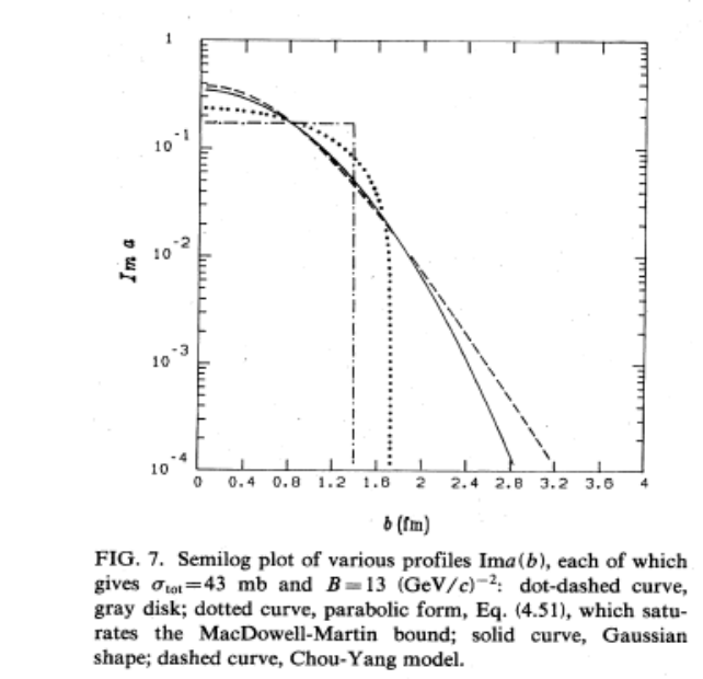
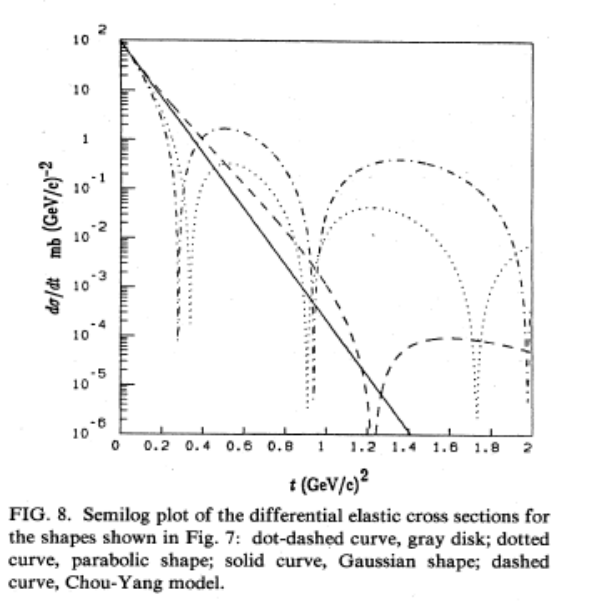
These figures bring to focus the basic difference between models with a Gaussian matter distribution and the others: the Gaussian shape leads to an exponential decrease in , with no wiggles or dips and bumps, whereas all the other distributions, grey disk, parabolic shape, or Chou and Yang model, exhibit a diffraction pattern with minima and maxima. Such difference among models persists till today.
5.3 Exponentials and parametrizations through Regge and Pomeron exchanges
The models in impact parameter space summarized so far underline the optical nature of scattering, without specific dynamical inputs, except for the hadron form factors. On the other hand, data on elastic scattering from ISR appeared to conform to a picture in which the elastic scattering amplitude obtains from Regge-Pomeron exchange. We shall examine some of such models. An additional group of models embeds Regge-Pomeron exchanges into the eikonal representation, thus ensuring satisfaction of unitarity, in addition to analyticity of the input Born scattering amplitude. Some of these models include QCD and diffractive contributions, as we shall discuss in a separate subsection.
5.3.1 The model independent analysis by Phillips and Barger (1973)
In 1973, Barger and Phillips (PB) proposed what they called a model independent analysis of scattering [321].
They propose two slightly different parameterizations, using a phase and two exponentials to describe the different slope of the cross-section as a function of momentum transfer in the range . The first, and more model independent parametrisation, is given as
| (5.3.1) | |||
| (5.3.2) | |||
| (5.3.3) |
Data from to () were fitted with this expression. The first exponential is seen to have normal Regge shrinking, namely
| (5.3.4) |
while the second exponential term is almost constant. The values of the parameters at each energy value are given in Table 10.
| B | D | |||||
|---|---|---|---|---|---|---|
| GeV | GeV | rad | ||||
| 12.0 | 4.84 | 7.47 | 7.33 | 0.370 | 1.66 | 2.06 |
| 14.2 | 5.25 | 7.53 | 7.79 | 0.305 | 1.69 | 2.12 |
| 19.2 | 6.08 | 7.96 | 8.00 | 0.232 | 1.73 | 2.12 |
| 24.0 | 6.78 | 7.97 | 8.07 | 0.194 | 1.76 | 2.16 |
| 29.7 | 7.52 | 7.82 | 8.41 | 0.175 | 1.81 | 2.16 |
| 1496.0 | 52.98 | 6.55 | 10.2 | 0.034 | 1.70 | 2.53 |
Notice that, with this parametrisation, the phase is fitted to be always larger than , so that the interference term is always negative and, in the energy range examined here, the fitted phase is energy dependent.
To understand better the role played by the energy dependence, the authors proposed a second parametrisation, clearly inspired by Regge phenomenology, i.e.
| (5.3.5) |
with an explicit energy dependence and the following parameter values, valid for all the energies: , in the units of Table 10.The results are presented in the two panels of Fig. 5.11 and the figure shows that the quality of the two fits is good and about the same for both models.


The PB parametrization applied to the preliminary TOTEM data at LHC7 gave the results discussed in [299]. This parametrization however misses the optical point by some 5-10%, but the description of the region is quite satisfactory. We shall return to the question of the very small behavior later.
In [321], it is also suggested that the “second exponential” can be identified with a term proportional to , valid, according to the authors, for all available data for . Following this suggestion, and mindful of the fact that the form factor dependence of the amplitude would contribute as , we have tried a slight modification of the Barger and Phillips model, which consists in substituting the second term in Eq. (5.3.1) with a term proportional to the 4th power of the proton form factor, namely to write
| (5.3.6) | |||
| (5.3.7) |
which leads to
| (5.3.8) |
When applied to LHC7 data, this parameterization would comprehend both the proposal by Donnachie [322, 323] (further discussed at the end of this section), who advocates a power law decrease of the type , as well as the fit proposed by the TOTEM collaboration, , with [280].
A discussion of how these two models, two exponentials and a phase or one exponential, a form factor and a phase, would be realized at LHC, reading data from [280], can be found in [299].
That the behaviour past the dip at LHC is consistent with an exponential was also noticed in [300].
One can see however that the expression
| (5.3.9) |
gives a value for below the data at all energies, including at LHC7, where the fitted value misses TOTEM datum by some 5%, but particularly so at low energy and that the t-dependence of the t for , while reasonably well described at LHC, is less so at lower energy values. These two points are connected, since we have already noticed that at very small values at ISR the slope seems to increase. An interpretation of this effect is given in the Durham model [224], with pion loops contributing to the effective Pomeron trajectories at very small -values [324] and shall be discussed together with diffraction.
To overcome this problem and still provide a useful tool, we have proposed an empirical modification of the original BP model amplitude [307], i.e.
| (5.3.10) |
and
| (5.3.11) |
With free parameters in Eqs. (5.3.10, 5.3.11), the resulting analysis of elastic data at LHC7 is shown in Fig. 5.12. This figure includes a comparison with a parametrization of the tail of the distribution given by the TOTEM collaboration (dotted line). Such a parametrization, , was suggested in [296], and recently proposed again in [323], where it is shown to describe large data from ISR to LHC8, and both for and , as we shall discuss shortly.
Before leaving this model, we remark that the dip present both at lower and higher energies in is only a faint appearance in . The simple expression for the amplitude with two exponentials and a phase may still be a valid phenomenological tool also for , but one cannot draw any conclusion about the energy dependence of the parameters from this channel; as one gets close to the dip, and the first term dies out to zero, non leading terms, present in and not in fill the dip and probably need to be added to the original model, namely one has, as pointed out in many models, a situation such as
| (5.3.12) |
where depends on the Regge trajectories exchanged in the channel, including a possible odderon, as we shall see later.
Concerning the coefficient , we notice that in the two exponential model just described, this coefficient is related to the slope as defined in Eq. (5.1.5) through the relation
| (5.3.13) |
The PB model can be seen as an attempt to describe the elastic differential cross-section without appealing to unitarity. It was defined as model independent analysis, but it could also be understood as a modeling of elastic scattering through Regge and Pomeron exchanges. Since then many fits to data have appeared with a few Pomerons or many Reggeons and Pomerons. We shall next look at recent contributions, along these lines, by Donnachie and Landshoff.
5.3.2 Soft and hard Pomeron exchanges in Donnachie and Landshoff model
In [322, 323] the authors stress that the data from the TOTEM experiment do confirm the results of Regge theory, which is in many ways a major success of high energy physics. At high energy however such success depends on interpreting a power law as the ultimate solution, and at the end, as we shall see, resulting in using models to describe the details of the data. Indeed if one believes that the Froissart bound is actually reflecting the existence of confinement, power laws, which contradict the Froissart bound, must at a certain point give up to the true asympotic behaviour.
In Ref. [322] a hard Pomeron had been invoked to describe LHC7 data, but in the more recent contribution of Ref. [323], this is not considered necessary. Instead, a double Pomeron exchange is seen to provide a better fit, as they show. Of particular interest here is the fact that in both their modeling of the data, it is triple gluon exchange, term, which describes the decrease of the elastic differential cross-section past the dip in the tail region. This is a purely real contribution, which behaves as and could be energy independent.
In [322] three different types of data are analyzed:
- •
elastic scattering at the ISR,
- •
HERA data for the proton structure function at small , used to determine the hard and soft pomeron powers
- •
the TOTEM data for both the elastic differential distribution as well as the total cross-section.
The expression used to fit the LHC data is
| (5.3.14) | |||
with real and positive. The 4 Regge trajectories are parametrized as
| (5.3.15) |
with treated as free parameters and
- •
is the hard Pomeron, with
, which, they find, works well - •
is the well known soft Pomeron, with
, - •
is the degenerate trajectory, with
- •
corresponds to trajectory, with
The normalization of the amplitude is
| (5.3.16) |
The parameters are related to the proton structure function. Thus a simultaneous fit to the HERA data and to LHC7 gives the figures shown in Figs. 5.13 and 5.14, where the differential elastic cross-section is computed without and with a hard Pomeron, respectively.


The difference between the two figures is due to the fact that, since the total cross-section cannot come out right without a hard pomeron, a hard Pomeron is added to obtain the total cross-section as given by TOTEM. This gives the parameters for the hard pomeron as and .
At large , the authors add a real term to the amplitude of the type which they understand as due to triple gluon exchange [325, 296]. In order to make it finite at a possible expression is proposed as
| (5.3.17) |
It is pointed out in this paper that in order to correctly model the dip, both the real and the imaginary parts must become very small at the same value of .
In the more recent contribution [323], where no hard Pomeron is invoked, the amplitude is given as three single Pomeron exchange terms, one double exchange and a triple gluon term. We show a representative fit of the LHC7 data from this paper in Fig. 5.15.
Each one of the three single-exchange terms is related to a trajectory , with
| (5.3.18) |
for the / amplitude, respectively, , and is a form factor. The three trajectories are parametrized as
| (5.3.19) |
To these single-exchange terms, a double Pomeron exchange, term, is then added. It corresponds to a trajectory
| (5.3.20) |
but the corresponding amplitude term is non just a power , and additional logarithmic terms appear at the denominator.
The tail of the distribution is given by triple gluon exchange [296], and is such that at large one has
| (5.3.21) |
A joining with the other parts of the amplitude is obtained by trial and error, as the authors say, and is parametrized with
| (5.3.22) |
The small in the Coulomb region is included as
| (5.3.23) |
The description of data from ISR to LHC for is very good, less so the description of data, but this is common to many present fits. The values for the 12 parameters which give the best fit to total and elastic data are given in the paper, with in particular .
5.3.3 The model by Schegelsky and Ryskin
In [62], the emphasis is on the small- behaviour and a concern that the elastic slope may not be just a simple linear power in . The authors start with the usual Regge and Pomeron parametrization for the elastic scattering amplitude, namely
| (5.3.24) |
where the first term corresponds to the Pomeron, the second to a Reggeon and would be negligible at high energy. The differential elastic cross-section at high energy thus takes the form
| (5.3.25) |
where the slope of the Pomeron trajectory accounts for the growth of the interaction radius caused by a long chain of intermediate (relatively low energy) interactions. Agreement with data, with an elastic slope given by
| (5.3.26) |
is obtained by assuming a Gaussian type behaviour for the form factors . The second term in Eq. (5.3.26) is supposed to be universal, and the value obtained by examining fixed target experiments, i.e. up to , is given as . On the other hand, the original analysis by Donnachie and Landshoff [139] at would lead to .
This discrepancy points to the fact that the energy dependence of the elastic slope may be more complicated than a simple logarithm. The first idea is that as the energy increases, multiple interactions take place. In Regge-language, these multiple interactions are described by multiple Pomeron diagrams.
One important point is that in impact parameter representation, as the energy increases towards the black disk limit, the imaginary part of the elastic scattering amplitude . However, while asymptotically going to the black disk limit, at the periphery the amplitude is still growing. This leads, according to the authors, to an effective growth of the slope. The reason is that the continuing increase of the amplitude at the periphery of the impact parameter space implies an increasing radius. In this way the authors understand the discrepancy between their result for relative to Donnachie and Landshoff. They also provide another way to understand this behaviour, namely the interplay between one and two Pomeron exchanges, which have different signs, so that as the two Pomeron effect increases, the amplitude drops more rapidly.
Assuming an -dependence different than the simple logarithm of Eq. (5.3.26), may explain why . The authors propose
| (5.3.27) |
so that, if one rewrites Eq. (5.3.27) as
| (5.3.28) |
one would obtain . To determine the coefficients, the authors plot the results from a series of experiments, as we show in the left panel of Fig. 5.16.


For , the coefficient is consistent with zero, while, for , the authors obtain . Since is consistent with zero, the authors propose to drop this term altogether and refit the data with only a term. This fit gives .
Their result is then discussed in light of the fits done by Block and Halzen in [262] and the possible saturation of the Froissart bound. Unlike Block and Halzen, the authors here do not think that the black disk limit is yet reached, and believe the proton to be still relatively transparent, so that , with , is not yet at its geometric value. One word of caution is however put forward by these authors, namely that the non linear logarithmic rise of the elastic slope is basically determined by the recent TOTEM measurement of . Up to and including the TeVatron measurement, a linear logarithmic energy rise for is in fact actually still compatible, as one can see from Fig. 5.16.
5.4 Analyses with Pomeron, Odderon and Regge exchanges
The dip structure has been connected to C-odd exchanges in the t-channel, phenomenologically referred to as the Odderon. The existence of such a state is predicted by QCD and has been advocated in particular by Nicolescu, also in collaboration with other authors [326, 214].
As we have mentioned in Sect. 4, the QCD treatment of the Odderon began in 1980 [215] [217]. It was examined extensively by Bartels and others in non-abelian gauge and color glass condensate theories. Present QCD studies of the Odderon trajectory focus on NLO contributions [219] and properties in the strong coupling limit[220]. Still, the major question to face is whether and how to detect its presence in LHC experiments and this takes us to the many phenomenological analyses which include Reggeons, Pomerons and Odderons..
5.4.1 Phenomenological analyses with and without the Odderon contribution
To discuss the proposal to detect the odderon at RHIC and LHC by Avila, Gauron and Nicolescu (AGN2006) [212], we start with the model by Avila, Campos, Menon and Montanha (ACMM2006) which incorporates both the Froissart limiting behavior as well as Pomeron and Regge exchanges [213].
In [213], the elastic amplitude is normalized so that
| (5.4.1) | |||
| (5.4.2) |
Although, unlike the total cross-section, both the real and the imaginary parts of the scattering amplitude enter the elastic differential cross-section, in the small -region, , the cross-section can be expected to be still mostly imaginary. The steep decrease in this region region can be empirically parametrized in terms of an exponential, i.e. one writes
| (5.4.4) |
Experimental data suggest that their energy dependence can be parametrized in terms of polynomials in . The difference between and is then introduced as :
| (5.4.5) |
The above parametrization implies parameters, having imposed the constraint
| (5.4.6) |
which is valid when the Froissart bound is reached and can be considered a generalized form of the Pomeranchuk theorem [213].
Concerning the real part of the amplitude, the authors make use of the first order derivative dispersion relations for the even/odd amplitudes, defined as
| (5.4.7) | |||||
| (5.4.8) |
which lead to
| (5.4.9) | |||
| (5.4.10) |
The validity of the above expressions only extends to a region and depends on the value chosen for . In the subsequent fit to the experimental data, different values of are considered, leading to different parameter sets.
The above parametrization, applied to the vast set of lower energy data up to the Tevatron, gives the result shown in Fig. 5.17. We see that, for the energy , the parametrization does not show existence of a dip.

The above approach has been discussed because its no dip at LHC result in contrast with the TOTEM measurement, can falsify some of the assumptions, or lead to the need to introduce the Odderon, as done in a subsequent work with Nicolescu, as we discuss next.
Avila, Gauron and Nicolescu (AGN2006) [212] examine the data in light of the possible existence of the odderon, a QCD effect corresponding to a singularity in the complex J-plane at at in the amplitude , which is odd under crossing. The odderon is considered a non-leading QCD effect, which can only be detected in the elastic differential cross-section. In this analysis, its contribution is parametrized according to the properties of a number of Regge, Pomeron and Odderon trajectory exchanges, in the context of total cross-sections saturating the Froissart bound. With such parametrization, at LHC energies a dip is expected both for and scattering, something which cannot be proved experimentally at LHC. In [212] the suggestion is advanced to try to check the presence of the dip at RHIC, namely at .
The AGN2006 analysis describes the ISR data at where both and elastic differential cross-sections were measured. At this energy, while shows a dip, does not, and the model with the Odderon describes these features well. At and , where only scattering was present, the dip has morphed in a break in the slope, with not much difference between the two processes, with the curve remaining slighly higher. At , the break is predicted to be more pronounced and at the Tevatron energies there is the hint of a dip developing, with points remaining higher. Until recently, experimental data at the Tevatron did not go beyond . Presently published data from the D0 Collaboration [327], plotted in Fig. 5.18, indicate a pronouced break in the slope (as at ), possibly even a dip. This would correspond to the fact that the terms from Regge exchange are becoming increasingly negligible.

There are no predictions for LHC7, but at the dip is now predicted both for and .

At LHC running at (LHC14) the position of the dip is expected at , to be compared with the position at the ISR at and the position at LHC7 reported by TOTEM at .
We will discuss now in detail the parametrization in [212]. The starting point is the maximal asymptotic behaviour of the total cross-sections, consistent with data, i.e.
| (5.4.11) | |||||
| (5.4.12) |
According to [212], the choice of a maximal behaviour of the total cross-section is not necessarily implying that the imaginary part of is also maximal, i.e. that , but, the authors argue, it is the natural choice that strong interactions be as strong as possible. With this assumption, a parametrization for the two, even and odd crossing, amplitudes is prepared and then determined by comparison with the data.
These authors start with a general form for the hadronic amplitudes compatible with Eq. (5.4.12). Their strategy is to consider both the existence and the non existence of the odderon, parametrizing all the existing data (832 points when the paper was written) for both processes and for the quantities and . After choosing the best description for the existing data, the model is applied to predict future data and to recommend experiments which might measure the difference between the two amplitudes and . The expressions for these even and odd amplituds are written as sum of Pomeron and Reggeon contributions, following general theorems given in [328, 329, 292], namely
| (5.4.13) | |||||
where the upperscript correspond to a polynomial in , with
| (5.4.14) |
maximally increasing as with exponential dependence, is the contribution from the Pomeron Regge pole, the Pomeron -Pomeron Regge cut, corresponds to the secondary Regge trajectories, the reggeon-Pomeron cut. For the odd under crossing amplitude, represents the maximal Odderon contribution, also increasing as , is a minimal Odderon Regge pole contribution with , is a minimal Odderon-Pomeron cut, a secondary Regge trajectory associated with the particles and , a reggeon-Pomeron Regge cut.
In [212] the no odderon case is obtained by choosing parameters such that all the three amplitudes with contributions from the odderon are zero, i.e. . Because of the contribution from the Regge and the Reggeon-Pomeron cut, with
| (5.4.15) |
the amplitude is not zero, but it fails to give a good description of the ISR data at . The results can be summarized with the fact that, starting with the ISR data, the case without odderon does not reproduce the data at as well as it can do with the Odderon. According to the authors this is due to the fact that the -dependence of these two remaining terms is constrained by the parameters of the Regge and Pomeron trajectories, which are non-leading and fail to interfere with the even amplitude in the correct way.
Turning to the other case, namely the odderon being present, the model can count on twelve more parameters, which add to the 23 parameters determining the amplitude.
Numerically, it is now possible to do a good fit to ISR data which show the clear difference between and , with and without the dip. At LHC 14 TeV, the dip is fully in place, but, unlike intermediate energies, it would be present in both processes, and the difference between the two cross-sections is small. The predicted dip is at and the cross-section after the dip rises to .
A pattern of oscillations is observed to develop in the difference for and . with two minima, one around and the other around . In Fig. 5.20 we show the fit to the differential cross-section at ISR and the predicted difference.


In a subsequent paper [330] the model is extended to higher values of . They define as the standard data set the data set proposed by Cudell, Lengyel and Martynov [331]. To generalize the results beyond the range new terms are added to the parametrization originally proposed, namely
- 1.
which behave like and growing like . The motivation for was advanced to include the Odderon 3-gluon exchange, with elementary gluons.
- 2.
a term which has a role as “cross-over term” for very small
- 3.
two linear functions of the type multiplying the maximal odderon and the Odderon pole term, and which are necessary to describe the smallness of the Odderon forward coupling at present energies.
With these many parameters the fit is now very good and the model predicts a dip at 14 TeV around and a shoulder around . They note that at LHC energies the exponential behaviour of is no longer valid.
5.4.2 Jenkovszky’s Pomeron/Odderon Dipole model
We now discuss the contribution by Jenkovszky with different collaborators from [335, 336] and references therein. The model described in [336] extends the Donnachie and Landshoff model, to include the dip-bump structure of the differential elastic cross-section, non-linear Regge trajectories, a possible Odderon, i.e. C-odd asymptotic Regge exchange. The extension should also be such as to be compatible with and -channel unitarity. The authors recall that the first attempt to reproduce the dip-bump structure was done through the Chou and Yang model [320], whose major drawback is that it does not contain any explicit energy dependence. As mentioned, at the beginning of this section, the Chou and Yang model describes an impact parameter distribution obtained from the proton electromagnetic form factor. In the Chou and Yang model, just as in the eikonal models in general, the dip-bump structure is obtained because of the zeros of the imaginary part of the amplitude, induced by the Fourier transform from space. In [336], the pattern of the parametrization proposed by Barger and Phillips in 1973 [321], already discussed, is followed. The amplitude is normalized so that
| (5.4.16) |
with constants to be determined from the fits, and the amplitudes written such as embodying the Regge-Pomeron description, itself reflecting the collective processes participating to high energy scattering.
The model in [336] is based on four contributions to the scattering amplitudes for and , and the amplitudes are written as a sum of Regge pole amplitudes, namely
| (5.4.17) |
where stand for the Pomeron and Odderon contribution respectively -even and -odd with intercept , and , again -even and -odd and . The Pomeron and the Odderon are treated on the same footing, their parameters to be determined by the fit to the data. For Pomeron and Odderon, a dipole expression is chosen, with a non-linear trajectory, i.e.
| (5.4.18) | |||
| (5.4.19) |
with . For the Pomeron trajectory, both non linear and linear cases are considered, while the Odderon is taken to lie on a linear trajectory, similar to the reggeon trajectories for and . The adjustable parameters are the trajectory slopes and intercepts, the constants and and , which quantify the presence of absorption.
The fits to the usual set of observables, differential elastic cross-section, total cross-section and parameter, lead the authors to conclude that the Odderon contribution is necessary in order to correctly describe the dip-bump structure from ISR to the Tevatron. It should be noticed that in this model there are no wiggles beyond the first dip, since this model does not use the eikonal form for the amplitude, but directly parametrises it in the plane. For LHC, we reproduce their predictions in Fig. 5.21.

More particularly, the conclusions from this model in [336] are the following:
- 1.
A single shallow dip is expected at LHC followed by a smooth behaviour
- 2.
The Odderon, described as a dipole, with a positive intercept and almost flat behaviour in is indispensable to describe the dip-bump region
- 3.
the diffractive minimum in at LHC7 is expected at , receding to at LHC14
- 4.
the contribution from the non-leading Regge trajectories can be neglected in the LHC region.
Recently, the possibility to extract the odderon and the pomeron contribution from and data has been revisited in [337]. After early results from LHC8 have been published, the model has been applied [338] to include a threshold singularity in the Pomeron trajectory, requested by channel unitarity and related to the pion pole to account for the non linear slope at very small -values, as reported by the TOTEM collaboration [284]. The possibility that the amplitude reflects a square root singularity was suggested long time ago [324, 339], and is also present in the work by Khoze, Martin and Ryskin, discussed in 5.6.3.
5.5 Eikonal models driven by Pomeron exchanges, parton dynamics and QCD inspired inputs
Eikonal models allow to satisfy unitarity and comply with the asymptotic requirements of the Froissart bound. Models using this formulation differ depending on the particular dynamical input determining the eikonal function. We shall briefly illustrate some results from models which include partonic descriptions of the proton, such as the Islam model, the so-called Aspen model, and resummation of many Pomeron-like exchanges. We also include in this subsection the eikonal based model by Bourrely, Soffer and TT Wu. In a separate subsection we shall illustrate QCD models which specifically include diffractive processes and derive their input from QCD evolution equations, notably the BFKL approach.
5.5.1 Quarks and gluons in the Islam model
A model based on the eikonal representation but reflecting the internal structure of hadrons is given by the Islam model [340, 341, 342].
In Islam’s original model for elastic scattering, the scattering is described as a two component process: the first giving rise to diffractive scattering where the two pion clouds surrounding the scattering nucleons interact with each other, whereas the second hard scattering process, dominating at large scattering angle, takes place via vector meson exchange, while the pion clouds independently interact.
In a more recent paper [341] the model evolves into three components, a soft cloud, a hard exchange at low c.m. energy and a hard component at high energy, identified with the BFKL Pomeron. Let us see how this picture is realized, also based on Luddy’s presentation at Blois 2009 [343]. This model is lately referred to as Condensate enclosed Chiral-bag Model, and can be seen pictorially from a drawing of this presentation, Fig. 5.22.

In this version of the model [341], a hard scattering term brings in four new parameters, namely the relative strengths between the exchange term and the hard term, the hard pomeron intercept , the black disk radius and the mass which determines the size of the quark bag. In total this model has 17 parameters which can be fixed giving a quite satisfactory description of the total and differential cross-section, at various c.m. energies and of the parameters.
In [343, 344], as in the previous papers, the proton is described through three basic elements: an external cloud of pairs (sea quarks), an inner shell of baryonic charge and a central quark-bag containing the valence quarks. The external cloud and the inner shell have an obvious connection to QCD phenomenology, a pion cloud or some gluon condensate and the valence quarks, while one nucleon probes the baryonic charge of the other via -exchange. Thus the picture is:
- 1.
At very small values of the momentum transfer, the scattering is diffractive and we see the interaction of one cloud of one nucleon interacting with the cloud of the other nucleon
- 2.
then the -exchange starts dominating
- 3.
at even higher values, it is quark-quark scattering which takes over, i.e. pQCD.
The diffractive contribution
| (5.5.1) |
is built phenomenologically with a diffraction profile function given as
The above profile function renders the asymptotic behaviour of the total cross-section through the function , with an even crossing energy dependent coupling constant. Through the assumed energy dependence of the radius , the function gives rise to an asymptotic energy dependence which saturates the Froissart bound. It is thus possible to obtain the following results, with corresponding asymptotic theorems in italics :DE
| (5.5.2) |
where AKM stands for Auberson, Kinoshita and Martin scaling [292]. The contribution from -exchange is written as
| (5.5.3) |
where the first factor represents the absorptive effect from soft hadronic interactions in exchange , and the refers to and scattering. The squared form factor in the amplitude indicates that one is probing two baryonic charge distributions. Finally the last term, which dominates at larger values, is due to valence quark scattering, with the quarks interacting via reggeized gluon ladders, described through the BFKL Pomeron. This initially single valence quark scattering is then unitarized. We show these predictions in Fig. 5.23, where the different contributions are indicated separately.

In 2015, the model took a significant step forward, with incorporation of polarization of the outer quark-antiquark cloud region of the proton by the enclosed baryonic charge as described in [345].
5.5.2 The eikonal model by Bourrely, Soffer and Wu
Another model of interest is due to Bourrely, Soffer and Wu (BSW). In [166], the total as well as the differential cross-sections are discussed. Recent results and a comparison with LHC data can be found in [346, 347]. We show in Fig. 5.25 their pre-LHC predictions at various energies for the elastic differential cross-section.

This model follows in the steps of the very early work by Cheng and Wu. A particularly clear description of how the impact picture developed after the work by Cheng and Wu (CW) can be found in a short review paper by Jacques Soffer [162] and also in [163]. It is recalled that QED was the only known relativistic quantum field theory in the late ’60s and that CW introduced a small photon mass in order to avoid what Soffer calls unnecessary complications. After a brief introduction to the CW results, Soffer [162] describes the model developed together with Bourrely and Wu, starting with the elastic amplitude for proton scattering namely
| (5.5.4) |
where the signs refer to and respectively. The hadronic amplitude is given by and the factor has been factorized out of the Coulomb amplitude . For the latter, one has
| (5.5.5) |
where is the fine structure constant, is the phase introduced by West and Yennie [119] as
| (5.5.6) |
being the Euler’s constant and . is the proton electromagnetic form factor, and the model chosen by Soffer in [162] is
| (5.5.7) |
The usual quantities are defined accordingly as
| (5.5.8) |
and the hadronic amplitude is obtained from the impact picture [164] as
| (5.5.9) |
The eikonal function is split into two terms, reflecting different dynamical inputs, namely
| (5.5.10) |
where includes the Regge contribution important in the low energy region and is different for and , whereas the second term is the same for both processes and gives the rising contribution to the total cross-section. This term is factorized into energy dependence and impact parameter dependence as
| (5.5.11) |
with the energy dependence given as in the CW model. Thus the model exhibits a Pomeron energy dependence given by a complex crossing symmetric expression
| (5.5.12) |
where is the third Mandelstam variable. At high energy and small momentum transfer, the real and imaginary parts of the amplitude can be obtained through the substitution . As for the essential impact parameter dependence, and hence the -dependence, this is parametrized through an expression similar to the proton electromagnetic form factor, namely the Fourier-transform of is
| (5.5.13) |
This model had six parameters, of which two, and , related to the energy dependence, and the other four, and describing the impact parameter dependence.
Including the LHC7 data, the values obtained for the six parameters are given in Table 11, from Soffer’s contribution to Diffraction 2012 [346].
| c=0.167 | c’=0.748 |
|---|---|
The recent discussion of the model in [346] gives the description shown in Figs. 5.26, 5.27, respectively for the scattering amplitude and the differential cross-section. Fig. 5.27 shows that the tail of the distribution after the dip reflects the usual oscillations characteristic of eikonal models.


We note that the -dependence, hence the -dependence, is obtained through the form factor , which is not the nucleon factor nor a convolution of two nucleon form factors, as it would be in the eikonal mini-jet models or the Glauber models. This form factor is independent of the overall energy.
5.5.3 Many Pomeron structures in eikonal models
We discuss here four papers by Desgrolard, Giffon, Martynov, Petrov, Predazzi and Prokudin, who have worked together in different combinations. These authors have been involved in a precision analysis of resonances and the forward region, as in Desgrolard, Giffon, Martynov and Predazzi [349], but they also deal with the elastic differential cross-section [350]. In Petrov and Prokudin [351] the three Pomeron model is introduced. Then the model is again discussed in [352] and the Coulomb interference problem is picked up by the same authors, this time with Predazzi in [353] and before in [352] .
The main point of this approach is the need to go beyond one or two Pomeron pole description of the elastic differential cross-section, and allow for many Pomerons. Let us begin with Desgrolard, Giffon, Martynov and Predazzi [350], which contains in its introduction a good description of the state-of-the-art in the year 2000, at the time LEP was closed and construction for LHC started.
This model is based on eikonalization of the input Born amplitude. Namely, the scattering amplitude will be given through the eikonal function , and one has the usual set of equations
| (5.5.14) | |||||
| (5.5.15) | |||||
| (5.5.16) |
The eikonalized amplitude in space can be written through the Fourier-Bessel transform
| (5.5.17) |
of the function which is to be defined in terms of an amplitude , which is the Fourier transform of the Born amplitude in space,
| (5.5.18) |
The next problem is the nature of the resummation procedure which takes one from the Born amplitude to the full amplitude. The Born input for the crossing-even and crossing-odd amplitudes
| (5.5.19) |
will be determined by the available data on the total cross-section, the differential elastic cross-section and the ratio . The even part is parametrized through the contribution of a Pomeron and an -reggeon, while the odd part is an Odderon and an -Reggeon, i.e.
| (5.5.20) | |||
| (5.5.21) |
For the Reggeon, the standard form is used, namely
| (5.5.22) | |||
| (5.5.23) |
where R stands for the - or -trajectories. For the Pomeron, the authors investigate two possibilities, a monopole (M) or a dipole (D), respectively
| (5.5.24) | |||||
| (5.5.25) |
As for the Odderon, the chosen form is
| (5.5.26) |
with M or D standing for a monopole or a dipole. It should be noticed that in this paper, the authors state that for the ratio to be fitted by the data, it is necessary that the Odderon contribution vanishes at .The trajectories are all taken to be linear in , i.e.
| (5.5.27) |
There is a relationship between eikonalization and unitarization [354, 355, 356], which gives the following constraints
| (5.5.28) |
Most fits give .
Once the Born amplitude is stated, the authors discuss different eikonalization procedures, one called Ordinary Eikonalization (OE) in which one puts
| (5.5.29) |
and the other is the Quasi Eikonal (QE) with
| (5.5.30) |
The explicit analytical form is
| (5.5.31) |
When , one obtains the OE. Still another form of eikonalization corresponds to the case when the weight is different for different terms. In the QE case, the various terms in the sum have the same weight, but one can consider the possibility that the terms have different weights, and this case is called the Generalized Eikonal (GE). The case with three ’s is discussed in detail, and fits are given. One observation here is the development of structures in the amplitude as a function of . Apart from the dip, there are oscillations, which are a consequence of the properties of the Bessel function from the Fourier transform. It is possible that some special feature of the eikonal may eliminate these oscillations, but in this model they are still present.
The authors discuss fits within the OE and the QE. They have more freedom to do a best fit with the GE with 2 or 3 parameters, and different cases for fixed or variable parameters for secondary reggeons are examined. The predictions of this model are shown in Fig. 5.28 from [350]. They emphasize three points:
- •
i) the presence of the Odderon contribution is necessary in order to describe the differential cross-section in the dip region and at large , the Odderon intercept consistently turns out to be negative from the fits,
- •
ii) the real part of the even amplitude has a zero at small -values, which moves toward as the energy increases, being at at . There are also other secondary zeros.
- •
iii) the eikonalized Odderon contributes to reproduce “perfectly” the large - region.

We now proceed to Petrov and Prokudin [351], entitled “The first three Pomerons”. This paper contains a short but useful introduction to various models, and well summarizes the state-of-the-art at the time. They observe that the large number of different models describing the scattering both at and for small -values hints to the fact that the most general way to deal with the problem is to introduce an arbitrary number of Pomerons. In [351] a first step is attempted to formulate an eikonal structure with many Pomerons. They begin with a three Pomeron structure, since, according to the authors, one and two Pomeron structures are inadequate.
Writing the unitarity condition as
| (5.5.32) |
where is the scattering amplitude in the impact parameter representation, the contribution of inelastic channels, the scattering amplitude in terms of an eikonal function as
| (5.5.33) |
with for . If the eikonal function has only simple poles in the complex J-plane, and the poles are parametrized as linearly rising Regge trajectories, modulo the signature factor, the contribution to the eikonal in is written as
| (5.5.34) |
in -space one then obtains
| (5.5.35) |
Three Pomerons are then introduced describing both and , as follows:
| (5.5.36) | |||||
where are the Pomeron contributions, the sign refers to even/odd trajectories, referring to , and even and odd trajectories. To restore analyticity and crossing symmetry, one substitutes with
| (5.5.37) |
and obtains the appropriate signature factors for the various terms contributing to the eikonal as
| (5.5.38) | |||
| (5.5.39) | |||
| (5.5.40) |
The trajectories are dealt with in the linear approximation, with a fit to the meson spectrum determining the parameters of the secondary Regge trajectories, and . The parameters defining the 3 Pomerons and the odderon contribution (a total of 20) are obtained by a fit to the total cross-sections, the parameter and the elastic differential cross-section, the latter in the range . Data for the total elastic cross-section are not included in the fit, but are a result of the model. This is not surprising given the fact that by fitting the total and the differential cross-section, one fixes both the normalization (optical point) and the slope. The fits require that the three Pomerons and the Odderon as well have intercept at larger than 1, which also implies that eventually there will be a violation of the Froissart bound, the slope of the odderon being very close to zero.The exercise is repeated with only two Pomerons, but the result is not very good: in this case, unlike the three pomeron case, the odderon trajectory is fitted to have intercept less than 1.
This paper also contains a good discussion of the connection of the model to string theory models, and to the predictions for BFKL.
Concerning predictions in the small region, the model indicates a dip at LHC around and a wiggle around . We show in Fig. 5.29 the predictions for the elastic differential cross-section at RHIC and at LHC.

5.5.4 The Aspen model
This model [149] is a QCD inspired version, applied to both proton and photon processes, of a description of the total and elastic differential cross-section based on a large amount of previous work. In the 1984 review, Block and Cahn [12] describe in great detail the constraints arising from unitarity, analyticity and crossing symmetry, introducing their own proposal for low and high energy parametrization. In the 2006 review, the phenomenological description is updated and an extensive presentation of the subsequent work is given [51]. Thus, in the following the term Aspen model refers explicitly to the description in Appendix A of [51]. A description of this model has already been presented in 4.9.3, here we recall its main points. The Aspen model uses the eikonal representation in order to ensure unitarity. It embeds in addition the constraints of analyticity, and crossing symmetry. The model includes both a crossing odd and a crossing even eikonal, i.e.
| (5.5.41) | |||||
| (5.5.42) | |||||
| (5.5.43) |
with , and
| (5.5.44) | |||
| (5.5.45) |
and
| (5.5.46) |
with having the same functional form as the other b-distributions, . All the -distributions are normalized to 1 and are obtained as the Fourier transform of a dipole. As for the cross-sections , their QCD inspired parametrization leads to the following large -behaviour:
| (5.5.47) |
For large -values, the even contribution is made analytic through the substitution
| (5.5.48) |
The two constants and are fitted to the data. At high energies, the odd eikonal vanishes like , since this is the term which accounts for the difference between and interactions, and at high energies such a difference should vanish. We show in Fig. 5.30 predictions for LHC14TeV and comparison of the model with the Tevatron data [145, 148].

We note that the predicted curve for LHC has a dip for and second (slight) dip (more like a wiggle) around . Presently, data up to at LHC7 show no other structure but the dip at .
The Aspen model has been the inspiration for the Dynamical Gluon Mass model [357] in which an energy dependent mass for the gluon is introduced to regulate the low- divergence in the mini-jet like eikonal functions. Recently, the group from Campinas has been concerned with the slope and the total and elastic cross-sections [289, 305]. The ratio is discussed as it can give information about different models and their asymptotic behavior. The question whether is growing linearly with as expected in Regge -Pomeron descriptions, or whether it would grow as [62] is addressed. This would be relevant in cosmic ray physics, where the ratio for proton-proton scattering defines the nucleon-nucleon impact parameter amplitude (profile function), and measurements of the cross-section are thus related to this ratio.
5.6 Models including the diffractive contribution to the scattering amplitude
Diffractive processes contribute to the total cross-section. They are inelastic processes with spatial correlations to the incoming particles, and their experimental definition depends on the type of experiments as well as on the cuts imposed on the final state. Theoretically the description of diffraction is rendered difficult because no exact theorems exist about its energy dependence. We show in Fig. 5.31 a compilation of data for the inelastic cross-section, from lower to very high energies, including some results from LHC experiments in different rapidity regions, and, in some cases, including extrapolations into the diffractive region. The spread of results at LHC7 reflects different experimental cuts and different extrapolations into the low mass region. The blue band gives the results from the soft resummation model, described in [42]. The blue circle at 14 TeV gives the Block and Halzen (BH) prediction [262].
Discussion of diffraction as distinct from both inelastic and elastic processes has a long history. Models for diffraction are present in the literature since early observations of final state particles appearing in configurations clearly correlated along the incoming projectile. As we shall discuss in the following, some of these models use a quantum mechanics formalism, inspired by Good and Walker decomposition of diffractive scattering [75], while the QCD approaches, such as those by the Durham [224] and Tel Aviv [358] group, use, in addition, a triple Regge formalism, to account for high mass as distinct from low mass diffraction. Recently a contribution by Gustafson to clarify the connection between some of these approaches has appeared [359].
In what follows we shall summarize some representative works concerned with the description of diffraction. We shall describe in some detail the contributions by Pumplin and Miettinen, started with some early work [58] and [360] and then followed by Pumplin with Miettinen [361] and by Miettinen and Thomas [72]. A clear description of this approach can be found in [73]. We shall also summarize the application of some of these ideas to mini-jet models by Lipari and Lusignoli [53]. The Regge-Pomeron analysis of diffraction performed by two groups, Durham (KMR) and Tel Aviv (GLM), will follow. A digression to the string theory Pomeron description by the Brown University group [265] will be included, as it is central to the Tel Aviv model. Many phenomenological analyses exist in the literature, for a recent analysis up to Tevatron data, a good summary can be found in the work by Dino Goulianos [362].
5.6.1 The Pumplin limit for diffractive processes
We now discuss the generalization of the break-up of the total cross-section into elastic, diffractive [360, 361] and inelastic components and how to obtain the so-called Pumplin limit [58], i.e. .
| (5.6.1) |
to be used instead of the black disk limit
| (5.6.2) |
Let the “b-wave” unitary matrix be decomposed as
| (5.6.3) |
If we define twice the imaginary part of the elastic amplitude by , Eq.(5.6.3) leads to the relation
| (5.6.4) |
valid for large if we neglect the small real part of the elastic amplitude.
The inelastic scattering sum in due to multi-particle production may be written as
| (5.6.5) |
If one assumes a statistically independent production of particles, one is led to the Poisson distribution
| (5.6.6) |
Then Eq.(5.6.4) leads to the well known eikonal form for the imaginary part of the elastic amplitude
| (5.6.7) |
with denoting the mean number of collisions occurring at a given and .
It is well to note that Eq.(5.6.4) has two solutions for :
| (5.6.8) |
The solution chosen in Eq.(5.6.7) is the smaller one which corresponds to as the mean number of collisions goes to zero. Hence,
| (5.6.9) |
We note in passing that this choice reduces the Martin-Froissart bound by a factor of 2. It also leads to one of our asymptotic sum rules [297, 298]
| (5.6.10) |
Using a phenomenological model such as the Phillips and Barger (PB) model of Ref. [299] for the elastic amplitude, one can see that experimental data at by the TOTEM group at the LHC support Eq.(5.6.10). The value is [299] at corresponding to . The other mathematically allowed possibility as that leads to is ruled out by data at present LHC energies.
The result of Eq. (5.6.8) however is incomplete. As discussed at the beginning of this section, if the eikonal function is constructed through a randomly distributed Poisson sum of incoherent scatterings, then the elastic ratio turns out to be larger than its experimental value at LHC, which is still , hence quite far from the black disk limit of Eq. (5.6.2). The reason behind this generic fact is that there is a non-negligible fraction of the inelastic cross-section, called diffractive which is not truly random but which maintains quite a bit of coherence with the scattered particles.
One type of contribution to single diffractive events occurs when one of the two scattering particles ends up in a state with the same internal quantum numbers with a close by mass but perhaps with a spin-flip (e.g., ) [73], while simultaneous break up of both scattering particles into diffractive states as defined above contributes to double diffraction. Even at high energies, such as at LHC7 for example, the contribution of the summed diffractive cross-section to the total is and hence it needs to be properly understood and formulated [361, 306]. References to other work on this subject can be found in [73, 53]. The analysis below follows these references in outline. Other references can be found in the Durham and Tel Aviv analyses, which include contributions coming from high mass diffraction.
The underlying essential physics of diffraction can be incorporated by supposing that the incident particles are in a superposition of “diffractive eigenstates” defined as
| (5.6.11) |
with giving the probability of finding the diffractive eigenstate in and . The interaction with the other particle produces a mixture of diffractive and non diffractive states
| (5.6.12) |
Hence with the breakup of only one particle of the initial state, the elastic amplitude becomes
| (5.6.13) |
where the average denotes an average over the diffractive state probabilities. As before neglecting the real part of the diffractive amplitudes, we would have the following expressions:
| (5.6.14) |
and
| (5.6.15) |
The sum of the elastic and diffractive differential cross-section (in b-space) reads
| (5.6.16) |
The basic result for the diffractive part of the differential cross-section in impact parameter space is obtained through Eqs. (5.6.15) and (5.6.16)
| (5.6.17) |
In words, is given by the dispersion in the absorption probabilities and hence it would vanish identically were all components of the initial state absorbed equally. If averages are taken over both incident particles, would include both single and double diffraction dissociation.
Now let us see how to obtain the Pumplin upper bound on . Since, by virtue of Eq.(5.6.9), the absorption probabilities , and , we have also that
| (5.6.18) |
This leads to the Pumplin inequality
| (5.6.19) |
and the integrated version of Eq.(5.6.19) leads to Eq. (5.6.1) for the ratio of the elastic + diffractive cross-section to the total cross-section. For scattering at ISR, which is over a half of the limit , predicted by the above Eq.(5.6.19). Presently, even at the highest energies, the limiting value of , as given by in Eq.(5.6.1) is closer to the experimental results than the black disk limit () for in Eq.(5.6.2), as we have seen from Fig. 5.5.
Pumplin [73] further observed that while -channel helicity conservation is a good approximation for the elastic amplitude such is not the case for diffraction dissociation.
To proceed further, one needs to formulate a model for the probability distribution for diffraction dissociation at high energies, which must respect several requirements:
- •
(i) for diffraction dissociation into a continuous mass spectrum, an analytic dependence on mass ;
- •
(ii) the constraints that all ;
- •
(iii) as (asymptotic constraint);
- •
(iv) as (asymptotic constraint).
As discussed next, a simple probability distribution meeting these requirements, which is amenable to an analytic treatment, is given by [72, 73]
| (5.6.20) |
with and the dispersion .
5.6.2 Specific models with a continuos distribution
In 1979 Miettinen and Thomas [72] discussed how to modify the Glauber eikonal formalism to include diffraction within a picture in which quarks and gluons are - with different spatial distributions- the constituents of a nucleon or a hadron. Since earlier analyses, in particular Good and Walker [75], it had been known that if the different components of a composite system have different distributions (absorption strengths), then inelastic states are excited and the elastic formula for the amplitude needs to be modified. The aim in [72] was to show that, taking into account fluctuations in the wave function, one can find the matter distribution. This is analogous to the distinction between a “charge distribution” extracted from elastic scattering and the proton charge distribution obtained through the proton electromagnetic form factor, extracted from scattering.
Their first step is to substitute the expression for the elastic amplitude between two hadrons and scattering at a distance
| (5.6.21) |
with a different amplitude, corresponding to the different possible configurations and in which the two hadrons find each other at the point of collisions,, i.e.
| (5.6.22) |
Calling the probability that the hadron is in a given configuration , the complete amplitude is obtained by averaging over all the possible configurations
| (5.6.23) |
The connection between the simple eikonal of Eq (5.6.21) and this description can be seen by writing Eq. (5.6.23) as
| (5.6.24) |
with the corrections to the simple eikonal embedded into the moments of the eikonal spectrum, i.e.
| (5.6.25) | |||
| (5.6.26) |
The connection to matter distribution in -space enters the eikonal function from the overlap of the average matter densities of the incident particles, i.e. the s-dependence is factorized into a constant and
| (5.6.27) |
To exemplify this model, Eq. (5.6.23) is written as
| (5.6.28) |
with the function defined by the probabilities . Now, the model becomes easy to solve under the hypothesis that the dependence of is only a function of the scaling variable . A simple function in the variable is considered, namely
| (5.6.29) |
which obeys the constraints
| (5.6.30) |
as requested by normalization and the first moment condition. One has
| (5.6.31) |
The integration is then done immediately, and the differential cross-sections in -space now become
| ; | (5.6.32) |
| (5.6.33) |
and
| (5.6.34) |
A few observations about this model are in order:
- •
(i) As , the earlier eikonal limits are reached since .
- •
(ii) For , Eq.(5.6.32) reduces to a “Fermi” distribution
(5.6.35)
Further extensions of this model can be found in the work by Lipari and Lusignoli [53], who use the mini-jet formalism to study the contributions to the inelastic cross-section from different hadronic configurations participating to the scattering. The authors start with a careful discussion of the relation between , the cross-section for producing a mini-jet pair, and , the total inelastic cross-section. Many authors have had difficulty in understanding why can be larger than : this is simply a reflection of the fact that the inelastic cross-section measures the probability of inelastic interactions between hadrons, whereas measures the probability of parton-parton collisions, so that, since includes at least one parton-parton collision, the ratio in fact describes the average number of mini-jet pairs produced in one inelastic collision and this can be quite large.
The authors next consider the average number of collisions , taking place at impact parameter ,
| (5.6.36) |
obtained from the relevant and -space distributions for each colliding parton, going into a hadron
, , where is a hard scale defining the applicability of the mini-jet perturbative description.
Since partons have a spatial distribution, this number depends on the probability that two partons,
separated by a distance , interact with each other, a standard practice in mini jet models.
Defining parton configurations in the colliding hadrons as and , the average number of mini-jet collisions is obtained by summing over all possible configurations, i.e.
| (5.6.37) |
Upon assumption of the factorization hypothesis
| (5.6.38) |
with a constant, real parameter independent of energy, the final result will be obtained by integrating over all values of the parameter , i.e. over all possible configurations, with a distribution given by a probability function which must satisfy the two conditions
| (5.6.39) | |||
| (5.6.40) |
where the second condition follows from Eq. (5.6.37). In this generalized Good and Walker structure the proposed final expression for the elastic amplitude is
| (5.6.41) |
with the simple eikonal case corresponding to . One can see that in such case the elastic cross-section includes both elastic and diffractive processes, so that in the simple eikonal case the inelastic diffraction contribution vanishes. The cross-sections in momentum space can now be explicitly written as
| (5.6.42) | |||
| (5.6.43) |
The differential cross-section inclusive of elastic and diffraction processes is calculated to be
| (5.6.44) |
An explicit model is built, with the probability function such as to satisfy the two conditions given by Eqs. (5.6.39) and (5.6.40), and chosen to be
| (5.6.45) |
as in [72]. The model depends upon the parameter . Upon performing the integrations in , one now has
| (5.6.46) | |||
| (5.6.47) | |||
| (5.6.48) | |||
| (5.6.49) |
The authors apply a parametrization of the mini-jet model to evaluate and predict the diffraction cross-section as a function of energy. Using the approximation
| (5.6.50) |
where refers to Target or Beam diffraction (D) and stands for double diffraction, one obtains
| (5.6.51) |
The last term in Eq. (5.6.51) includes an extra factor of 2 at the denominator, which corrects Eq. (85) of Ref. [53] . 77 7 Private communication by the authors. The results, for two different choices of the model mini-jet parametrizations, are shown in Fig. 5.32 in comparison with, then available, experimental data for single diffraction.

5.6.3 The Durham model by Khoze, Martin and Ryskin
The Durham model by Valery Khoze, Alan Martin and Misha Ryskin (KMR) offers a unified description of both soft and semi-hard interactions. This model, developed and continuously refined over many years, also with other collaborators, presents a QCD based Pomeron and parton phenomenology .
Recent papers by the Durham group [225, 226, 228, 363] describe data on multiparticle production and present differential cross-section analyses. The most recent version of the model uses a two and three-channel eikonal formalism and multipomeron exchange diagrams, incorporating both unitarity and Regge behaviour. In [363], the authors compared their original predictions, for the total cross-section and diffractive quantities, with TOTEM results. Adjustments of their earlier parameters appears in [226].
The essential ingredients in their model can be summarized as follows:
- •
Input Pomeron trajectory for soft and hard processes
- •
Eikonalization of the amplitudes
- •
Inclusion of diffractive processes
- •
Pion loop corrections to the Pomeron trajectory and small slope of the elastic differential cross-section
We shall briefly describe each of the first three items and then present their most recent phenomenology for the elastic differential cross-section. The inclusion of pion loop corrections will be treated separately in 5.6.4
- •
KMR1: Pomeron trajectory
This approach uses Reggeon Field Theory with a phenomenological soft Pomeron, while for hard interactions a QCD partonic approach is employed [227]. In the hard domain, where perturbative QCD and the standard partonic approach can be used, their Pomeron is associated with the BFKL singularity. In this perturbative domain, there is a single hard Pomeron exchanged with
| (5.6.52) |
It is noted that, although the BFKL equation should be written for gluons away from the infrared region, after resummation and stabilization, the intercept of the BFKL Pomeron depends only weakly on the scale for reasonably small scales. We reproduce in Fig. 4.10 their description of the connection between the intercept of the BFKL Pomeron and the value for . The figure shows how the intercept goes to a smooth almost constant behaviour as increases.
It is useful to note here that in mini-jet pictures, the value of corresponds with the mini-jet cross-section growing as . Thus, the bare KMR Pomeron plays a role similar to that of parton-parton scattering folded in with parton densities and summed over all parton momenta in the mini-jet model. Also, the bare slope is interpreted by KMR to be associated with the size of the Pomeron: . It is related to a hard scale, of the order of a few GeV, which can find its counterpart in of the mini-jet models. However, a precise correspondence still needs to be worked out.
On the other hand, the transition from the hard to the soft domain in KMR requires multi-pomeron exchanges through re-summation of soft -processes, thus lowering the scale of from the earlier hard to a soft scale. As a result, the BFKL Pomeron (i) bare intercept decreases and at the same time (ii) the slope increases by a factor from its bare value. Hence, one has an effective linear Pomeron trajectory such as the one given by the Donnachie and Landshoff parametrization, i.e.
| (5.6.53) |
KMR found empirical evidence for the above trajectory also in virtual photo-production of vector mesons at HERA.
Once again, we may find a correspondence of the change in the effective slope with the mini-jet model parameter through the observation that with .
We add here some further details regarding the “BFKL multi-Pomeron” approach. In the Durham model, the semi-hard particle production due to a single BFKL Pomeron is shown in the left plot of Fig. 5.33 from [364]. In this figure, Y is the rapidity interval. In (a), the of the partons are not ordered. The multiplicity of partons grows as with , and partons drift to lower values because of the running of the strong coupling constant. Notice the imposition of a cut-off , below which the cascade is forbidden to develop. In the central figure, (b), the structure of standard DGLAP-based MonteCarlo cascade is strongly ordered in : there is a driving process, in the central rapidity region, with the highest parton momentum and then, from the initial parton a cascade ordered from larger to smaller momenta. In this description, because of the singularity of the hard parton-parton cross-section , an energy dependent cut-off , called an infrared cut-off, needs to be introduced, as can be seen in PYTHIA 8.1 [365]. This cut-off is applied to the hard matrix elements, not to the parton cascade, which is stopped when . This cut-off depends on the chosen PDF set. The multiple interaction possibility is included through eikonalization, both for the DGLAP and BFKL description. Finally, the third figure, (c), includes absorption of low partons. An effective “infrared” cut-off’, limits the low- partons. This parameter which depends on , hence on the energy, is dynamically generated by the enhanced multi-Pomeron diagrams. Notice that the variable conjugate to impact parameter is the momentum transfer exchanged through the Pomeron ladder, while the variable is the transverse momentum of the intermediate parton.
We observe that this description follows from the classic GLR paper [221], where all gluons, those involved in hard scattering as well as the soft ones from radiation before the scattering, are considered on the same footing and described through evolution equations. This differs from an approach such as the soft- resummation model (BN mini-jet model), where soft gluons are treated as a separate factorized term from the hard mini-jet cross-section and resummed through a semi-classical procedure a’ la Bloch and Nordsieck (thus the name BN) [173].

- •
KMR2: Eikonalization of the scattering amplitufde
A simplified description of the model can be found in Appendix A of [224]. Starting with the usual expressions for the total and elastic cross-section in impact parameter space
| (5.6.54) | |||
| (5.6.55) |
the scattering amplitude is approximated as to be completely imaginary,. i.e. there is no real part.
With an effective (for illustration) Pomeron trajectory written as and vertex with exponential t-dependence , the starting point is
| (5.6.56) | |||||
| (5.6.57) |
Writing the amplitude in space as the Fourier transform of Eq. (5.6.57) with
| (5.6.58) | |||
| (5.6.59) |
this will be the input for the successive eikonalization procedure. In the case of a single channel the amplitude is written in term of the opacity function , i.e.
| (5.6.60) |
and then eikonalizing it, one obtains
| (5.6.61) |
with the opacity
| (5.6.62) | |||
| (5.6.63) |
A Good and Walker model to include low-mass diffractive dissociation is then developed as we shall now describe.
- •
KMR3: Inclusion of diffractive processes
The KMR approach to diffraction has evolved through the years, as more precise and higher energy data allowed further understanding. We summarize here some of the main ingredients of this model, whose most recent application to LHC data can be found in [227]. The authors begin with channel unitarity,
| (5.6.64) |
which, for real is satisfied by
| (5.6.65) |
One then writes the total elastic and inelastic cross-sections in impact parameter space as
| (5.6.66) |
which coincides with and brings the interpretation of as the probability for inelastic interactions. One notices that this interpretation is valid also in case of a non-negligible real part of .
Diffraction is defined as elastic scattering and low-mass proton dissociation, to distinguish it from high mass dissociation, the two types of processes being graphically described in Fig. 5.34 from [366]. Apparently the multi-Pomeron vertex controls both the saturation scale and high-mass dissociation.

The elastic differential cross-section is written as
| (5.6.67) |
In [367] a three channel formalism is used to describe the diffractive final states. Here we shall describe their two-channel formalism. In [224], the GW formalism is applied to the states , and the relative processes are introduced through a parameter which describes the effective coupling of the proton to the excited state , which will then decay into the observed low mass diffractive products. This is done by modifying the one channel description into a two channel one, i.e. by the substitution
| (5.6.68) | |||
| (5.6.69) |
The expression for the elastic amplitude thus modified to take into account the other channels, is now
| (5.6.70) | |||
| (5.6.71) | |||
| (5.6.72) |
In this model the opacity function is real and the amplitude acquires a real part through
| (5.6.73) |
where
| (5.6.74) |
The elastic proton-Pomeron vertex is parametrized as
| (5.6.75) |
with to be obtained from total cross-section.
- •
KMR high mass diffractive dissociation
The previously described decomposition of elastic scattering into GW type states cannot be applied to other types of inelastic processes where the final state has a continuous mass distribution, and does not have the same quantum numbers as the initial proton. As we shall also see in the case of the Tel Aviv model, triple-Pomeron exchanges are invoked for this type of events, with the cross-sections written as [224]
| (5.6.76) | |||
| (5.6.77) |
where is the coupling of the Pomeron to the proton and is the triple Pomeron vertex, obtained from a fit to low energy ISR data in [367]. and are the diffractive mass and the rapidity regions for double diffractive dissociation. To avoid these contributions to grow too rapidly and violate unitarity, saturation and screening must be imposed and survival probability factors are introduced, as described for instance in [224].
- •
KMR5 Recent phenomenology
After the general overview of the model, let us see how KMR apply it to elastic scattering at LHC. The basic building blocks of this model are now the three-channel eikonal formalism and multipomeron exchange diagrams, incorporating both unitarity and Regge behaviour. These physical requirements are parametrized through the following procedure:
- •
the dependent bare Pomeron intercept
- •
the bare Pomeron slope
- •
a parameter , which controls the BFKL diffusion in
- •
the strength of the triple-Pomeron vertex
- •
the relative weight of the diffractive states , determined by low mass diffractive dissociation
- •
the absolute value of the initial gluon density.
In [363], the authors compare their original predictions, for the total cross-section and diffractive quantities, with the TOTEM results, and, as stated earlier, they find the need to do new adjustments of the parameters, acknowledging 7 lessons, among which i) the fact that Totem result, , is higher than the others, CMS and ATLAS extrapolated -KMR believe it is due to low mass diffraction being higher than expected- and that ii) the ratio according to TOTEM and it cannot grow further. It is also acknowledged that to describe both the forward peak and the dip in the Durham model would need to introduce more parameters.
Adjustment of the parameters leads to new results, which we present in Table 12 from [226]. In this table, some KMR results for total cross-sections both prior to and including recent LHC data are shown.
| KMR pre-LHC7 | 3-channel KMR post-LHC7 | ||||||||
|---|---|---|---|---|---|---|---|---|---|
| energy | |||||||||
| TeV | mb | mb | mb | mb | mb | mb | mb | mb | |
| 1.8 | 72.7 | 16.6 | 4.8 | 0.4 | 79.3 | 17.9 | 18.0 | 5.9 | 0.7 |
| 7 | 87.9 | 21.8 | 6.1 | 0.6 | 97.4 | 23.8 | 20.3 | 7.3 | 0.9 |
| 14 | 96.5 | 24.7 | 7.8 | 0.8 | 107.5 | 27.2 | 21.6 | 8.1 | 1.1 |
| 100 | 122.3 | 33.3 | 9.0 | 1.3 | 138.8 | 38.1 | 25.8 | 10.4 | 1.6 |
This adjustment does ameliorate the situation, bringing their prediction quite close to most recent TOTEM result (at this writing) of [348].
Finally, recent descriptions of the elastic differential cross-section in the small range in this model is shown in Figs. 5.35 from [261], where a good description of how the various choices of formalism and parameters lead to the final results.

5.6.4 Very small behaviour
As already seen when discussing early measurements at ISR, various experiments reported an increase in the effective slope as approached zero. Such an effect is also seen when comparing LHC7 data with a phenomenological application such as the PB model revisited in [299, 307]. In this application, the two exponential model with a constant phase describes very well the region , but misses the optical point by some , signaling that the slope has a more complicated -dependence than that given by two exponentials. In general, attempts to describe the elastic differential cross-section near the optical point as well as the region past the dip encounter difficulty in describing the very small behavior. Presently, for LHC, a complete description is still lacking. From the theoretical point of view, it can be argued that this region should have contributions from the nearby thresholds in the unphysical region. The presence of this behavior at very small was advocated long time ago by Anselm and Gribov [324] as well as by Cohen-Tannoudji, Ilyin and Jenkovszky [339] and has been discussed by the Durham [224] and the Cosenza group [206]. In the following, we shall describe two attempts to include such effects, the one in the Durham model, and then a model proposed by Pumplin.
In the KMR model [224], the Pomeron trajectory of Eq. (5.6.52) is modified so as to include a very small effect. It is then called a two component Pomeron, consisting of three terms: the first two correspond to the usual linear trajectory describing the large scale, small impact parameter space , while the third term corresponds to pion-loop insertions and contributes a correction to the small -behaviour of the local slope. Such improvement over the linear Pomeron trajectory consists in introducing the pion loop corrections as prescribed by Anselm and Gribov[324]. The underlying physical idea is that pions being the lightest hadrons and the massless pion limit expected to be neither divergent nor negligible may provide observable corrections to the high energy slope of the elastic differential cross-section in the low momentum transfer limit. The expression proposed in [224] for the modified Pomeron trajectory is
| (5.6.78) |
where
| (5.6.79) |
with a semi-hard scale. The coefficient specifies the Pomeron residue to the total cross-section and
| (5.6.80) |
The above modification should then explain the very small- dependence of the effective slope of the differential elastic cross-section in the KMR model.
Reflecting the same type of singularity in low- elastic scattering, a model was constructed by Pumplin for the elastic amplitude in impact parameter space [74] which has the virtue that its Bessel transform, i.e., the elastic amplitude as a function of the momentum transfer , has branch points at the “right thresholds”: . Or, it can be modeled as the two gluon exchanges with a threshold at , where is the effective gluon mass.
Defining the elastic amplitude as
| (5.6.81) |
with
| (5.6.82) |
and
| (5.6.83) |
in the limit of a purely imaginary amplitude, which is a good approximation at large and small , Pumplin models the -dependence of the real , as follows
| (5.6.84) |
Using the decomposition
| (5.6.85) |
it is possible to invert Eq.(5.6.82) as a convergent power series given by
| (5.6.86) |
where and .
The series expansion for the elastic amplitude obtained in Eq.(5.6.86) converges rapidly and hence was proposed as quite useful for numerical computations. Also, the resulting slopes and curvature as a function of the momentum transfer are quite smooth. Remaining always in the small range, the model provides clear insights into the intricacies involved in obtaining accurate estimates of the slopes and curvatures as a function of . Let and be the forward slope and the forward curvature respectively. Below we quote their numerical values at and obtained in this model.
| (5.6.87) |
However, the sizable forward curvature cautions against accepting forward slopes obtained through single exponential fits. Another important point is that the curvature decreases strongly as a function of and changes sign at larger values of [299, 74].
5.6.5 Elastic diffraction in AdS/CFT
A strong emphasis on the embodiment of N=4 Super Yang Mills (SYM) physics [368] is part of the work by the Tel Aviv group, Gotsman, Levin and Maor (GLM). Because of this as well as of the intrinsic interest of the results, we now briefly discuss the approach to this problem in the context of the string/gauge theory developed in a series of papers by the Brown University group [265, 369, 370]. In these papers string/gauge duality has been employed to obtain interesting results for the Pomeron and the physics of elastic amplitudes for small .
A brief summary of results can be found in [371]. We can not give here a detailed description of the elegant formalism developed in [265, 369, 370], but present below results regarding the Pomeron intercept and a modified eikonal expression derived from . In their string/gauge theory, a scalar kernel as a function of the 4-dimensional invariants () and two bulk coordinates () from the fifth dimension, describes the Green’s function for the Pomeron. At its imaginary part reads
| (5.6.88) |
where the Pomeron intercept and are given by
| (5.6.89) |
with denoting the (large) ’t Hooft coupling constant. Three loop universal anomalous dimension of the Wilson operators in N=4 SUSY Yang-Mills model were first obtained in [372].
The expression for the imaginary part of the Pomeron propagator in Eq.(5.6.88) is similar to its corresponding form (in the weak limit) with its BFKL expression
| (5.6.90) |
where is the coupling constant for colours and . The above allows one to identify the correspondence between diffusion in the gluon mass virtuality given by in Eq.(5.6.90) with diffusion in the radial coordinate in the dual given by Eq.(5.6.88).
A reduction from to the needed propagator is then made. The latter depends on the chordal distance
| (5.6.91) |
and a dimension obtained for the physical spin operators occurring in BFKL/DGLAP:
| (5.6.92) |
where Eq.(5.6.89) has been used to obtain the last part of the above equation. Rewriting Eq.(5.6.92) as
| (5.6.93) |
one sees the symmetry . Hence, the function interpolates correctly (i) the value at giving the BFKL exponent as well as (ii) at corresponding to the energy-momentum tensor, the first DGLAP operator. A schematic representation of the relationship between and is shown in Fig. 5.36.

In the eikonal limit - for its domain of validity see [369]- the amplitude for scattering is written as
| (5.6.94) |
where are wave functions in the bulk coordinates and for Pomeron exchange, the generalized eikonal which is a function of () is given in terms of the Pomeron kernel by
| (5.6.95) |
In the limit where Pomeron exchange dominates, for and fixed, the eikonal reads
| (5.6.96) |
We may pause here to note the similarity and differences between this approach [for and moderate values of ] and the minjet model for total hadronic cross-sections. Also in the minijet model, the eikonal is proportional to with , a power of the total energy. However, in the minijet model, there is an exponential suppression for large which softens the power law growth in energy of the eikonal to powers in logarithms of energy of the elastic amplitude. Eq.(5.6.96) by contrast shows that the eikonal decreases only as a power of (or ) for large .
5.6.6 Gotsman, Levin and Maor: the Tel Aviv model
Recent descriptions of the model, which embody both Reggeon field theory and features from N=4 SYM gauge theory, can be found in [358] and in [373] where the diffractive peak at LHC and a summary of experimental and various model results are presented. High energy predictions for the mass distribution for both low and high mass diffraction can be found in [374].
For what concerns the elastic differential cross-section, from the optical point to past the dip, this model, similarly to KMR, describes the diffraction peak region where non-perturbative effects are dominant, and is not yet extended to the dip region.
To describe elastic scattering and include the different components of diffraction, single (SD), double (DD), and central (CD), low-mass and high mass diffraction, GLM introduce both a Good and Walker (GW) formalism with GW diffractive states, as well as non-GW processes.
In previous papers, whose reference can be found in [375], GLM had obtained a good description of the total and the elastic differential cross-section in the small region, with a given choice of the parameters defining the model. However, TOTEM data, in particular the rather high total cross-section value, were seen to require some changes in the parametrization [358]. Only one parameter seems however to be in need of a change, namely the Pomeron intercept . Other parameters need not to be changed, at least for a good description of high energy data, namely , where the present interest lies for this model. Before giving some more details on this model, we note the following input elements:
- •
both GW states and non GW states contribute to diffraction
- •
GW states contribute to both low and high mass mass diffraction, non-GW states only to high mass diffraction
- •
the amplitude in the eikonal is purely imaginary (the model is basically applied to the low -region)
- •
dipole form factors inspired by the proton form factors give the factorizable impact parameter dependence in the eikonal functions
- •
the s-dependence of the amplitudes comes from a single Pomeron with and intercept
- •
multi-Pomeron interactions described by enhanced and semi enhanced diagrams contribute to both GW and non-GW states
From the above one notices once more that the s-dependence of this model is the same as in mini-jet models, with a term , which is not associated with any explicit -dependence.
To take into account the whole spectrum of diffraction, GLM starts with a simple Good and Walker model with two eigenwave functions and . Upon diagonalization of the interaction matrix, the wave functions of the two observed states, a hadron and a diffractive state, the latter with mass small compared to the energy of the process, respectively and , are written as
| (5.6.97) |
with One then constructs the scattering amplitude in impact parameter space , with by solving the unitarity condition
| (5.6.98) |
i.e.
| (5.6.99) |
The eikonal function is the imaginary part of the scattering amplitude for a single Pomeron exchange, i.e.
| (5.6.100) |
where the Pomeron-proton vertex and is the Fourier transform of the proton-like form factor, a dipole with a scale . The zero value for the Pomeron slope, i.e. in GLM is understood to be in agreement with the results from N=4 SY as described previously, and is crucial as it allows for resummation of all pomeron interactions One sees that the impact space dependence in each eikonal depends on 4 parameters, the scales and in the form factors and the proportionality factors . The amplitude in Eq.(5.6.99) gives the multipomeron exchange contribution to the elastic and GW diffractive states.
The contribution of GW states is obtained using the formulae
| (5.6.101) | |||
| (5.6.102) | |||
| (5.6.103) |
with the corresponding cross-sections
| (5.6.104) | |||
| (5.6.105) |
To these contributions, one needs to add non-GW terms, which are produced by Pomeron interactions, in this model only considering triple Pomeron interactions. These contributions involve the triple Pomeron coupling . For single diffraction into a mass , with the authors obtain
| (5.6.107) | |||||
| (5.6.108) | |||||
| (5.6.109) | |||||
| (5.6.110) | |||||
| (5.6.111) |
where is the triple Pomeron vertex proportional to and
| (5.6.112) | |||
| (5.6.113) | |||
| (5.6.114) | |||
| (5.6.115) |
Similarly, one can obtain the amplitudes for double diffraction in terms of the functions written above, details can be found in [358]. The final result is that the integrated cross-section for single diffraction is the sum of two terms, the GW and non-GW, likewise for double diffraction. To obtain the integrated cross-sections however, a further step is required, i.e. the amplitudes and are multiplied by the survival probability factors .
The model cannot be solved from first principles, and needs phenomenological inputs such as the Pomeron intercept, the interaction vertices between the Pomeron with the two GW states, the low-energy amplitude of dipole-target interactions and one constant, for the GW states, .
The connection with is considered in [368] where the model is discussed in light of satisfaction of two ingredients: i) the need to deal with a large coupling constant, and ii) the requirement to match with high energy QCD. Thus, the Pomeron intercept can be large, but the slope of the Pomeron trajectory is very small. These results, already introduced in the previous papers, match with the fact that, in the strong coupling limit, theory has a soft Pomeron, i.e. the reggeized graviton with a large intercept, with , , the QCD coupling constant. The other important ingredient of the GLM model is the natural matching with perturbative QCD, where the only vertex that contributes is the Pomeron vertex: this is also understood in SYM since the Pomerons (gravitons) interact by means of the triple Pomeron vertex, which infact is small, at least . Another matching result between GLM and is that at large , only processes from diffraction dissociation contribute to the scattering amplitude. In GLM model, diffraction indeed plays also a large role, as discussed before.
The main ideas of this model can be summarized as follows:
- •
a double face Pomeron, with
- 1.
a large intercept, , a direct consequence of when becomes large
- 2.
a short distance behavior, indicated by a small slope , as a QCD matching prescription
- 1.
- •
Good Walker mechanism and triple Pomeron vertex
To the above, one needs to add an important crucial component of GLM description of diffraction, i.e. the survival probabilities for large rapidity gaps. From the eikonal formulation, the survival probabilities are obtained from the quantities
| (5.6.116) |
which represent the probability that the initial state does not break up after the scattering.
After the publication of the TOTEM actual data for the differential cross-section and confirmation of earlier results for total elastic and inelastic, GLM were able to consolidate their parameters, and present definite expectations for this model [358]. The detailed results for all the quantities of interest appear in the paper. These include and at in addition to , for which the separate values obtained for the GW and non-GW contributions are also listed.
We reproduce in Fig. 5.37 the fit to data in the small t-range for different energies up to LHC14. Since the model is only to be applied at vary small values, as one approaches the dip the model starts not to reproduce well the data.

Because of the importance of diffraction in this model, a warning is pronounced about the black disk limit in [375]. The model results indicate a very slow approach of the elastic amplitude to saturation of this limit, in good qualitative agreement with what we have noted elsewhere in this review, namely that the AUGER results for the inelastic cross-section indicates . To summarize, it is observed that present Reggeon models all introduce at least two different mechanisms for diffraction. In GLM, these two mechanisms are : i) the GW production of diffractive states with unspecified finite mass, independent of energy, and (ii) diffraction due to Pomeron interactions, with a dependence on the Pomeron parameter . In other models, there are distinctions between low-mass and high-mass diffraction, and central diffraction. A discussion of this point can be found at the end of Ref.[358].
5.6.7 A comment about soft gluons and diffraction.
Before ending this brief review of selected contributions present in the literature, we shall comment on the possible interpretation of diffraction in terms of soft gluon emission. In the BN model of [94, 95], the contribution to diffraction is not present. What drives the increase of the cross-section is the result of parton-parton scattering (mini-jets) dressed with soft gluon emission from the initial valence quarks. Eikonalization then re-sums multiple interactions, each one of them coming with its own cloud of soft gluons. The present version of this model does not explicitly include soft gluon emission from the spectator quarks. However, diffraction along the initial state protons in such a view should include both emission from the quarks participating to the scattering, but also from the so-called spectator quarks. When the proton is hit by the other hadron, quarks also undergo intra-beam scattering. Such emission is along the colliding particles. This is in agreement with the original view of diffraction a’ la Good and Walker where the target and/or the projectile dissociates into a state with no change of quantum numbers: the only gluon emission process which, by definition, does not change the proton quantum numbers is resummed soft gluon emission. This is the dynamical picture which should be addressed. If nothing else but diffraction a’ la Good and Walker is present, then this emission could be accompanied by a factor inhibiting parton-parton scattering, namely a survival probability factor.
5.7 One-channel mini-jet model for total, elastic and inelastic cross-sections
As just discussed in 5.6.7, our BN mini-jet model has not yet dealt with diffraction, being so far a one-channel eikonal model. However, this model can provide interesting insight in the distinction between correlated and uncorrelated inelastic processes, and what in included in in one-channel eikonal models.
Here we shall discuss the mini-jet contribution to total, elastic and inelastic cross sections, using a one-channel eikonal formulation
as described in greater detail in [57].
To construct the total cross section, mini-jets are embedded into the eikonal formulation. Starting with
| (5.7.1) |
and neglecting the real part in the eikonal at very high energy, the above expression further simplifies into
| (5.7.2) |
where . Notice that is a reasonable approximation for the scattering amplitude in -space at , where very large values of the impact parameter dominate and phenomenologically the ratio of the real to the imaginary part of the forward scattering amplitude . By properly choosing a function , all total hadronic cross sections, , , , etc., can be described up to currently available data [152]. In the vast majority of models, new data have often required an adjustment of the parameters which give .
In previous publications, we had proposed a band whose upper border gave a good prediction for LHC results. By updating the model and anchoring the parameter set to LHC results, one can now proceed to refine our predictions for higher energies, LHC13 and beyond to the cosmic rays region.
The eikonal function of the mini-jet model of [94, 95] is given by
The first term includes collision with , the second is obtained from the mini-jet cross section. The term is not predicted by our model so far and we parametrize it here with , obtained with a constant and one or more decreasing terms, and , the impact parameter distribution in the non perturbative term, obtained through a convolution of two proton form factors.
As expected, the second term in Eq.(5.7) is numerically negligible at energies . The perturbative, mini-jet, part discussed previously is defined with and is determined through a set of perturbative parameters for the jet cross section, namely a choice of PDFs and the appropriate . Since soft gluon re-summation includes all order terms in soft gluon emission, our model uses LO, library distributed, PDFs.
The results of the LHC updated analysis of the one-channel BN model have been presented in Fig. 4.19, where, as mentioned, the points are shown, but have not been used for the phenomenological fit, and values for extracted from cosmic ray experiments have not been used either. In this figure both ”old” densities such as GRV [97] and ”newer” ones such as MSTW [96] have been included and compared with other models [262] and one-channel model predictions such as in [261, 263]. Table 13 contains the points corresponding to our model results for both GRV and MSTW densities.88 8 An error in the arXiv posted paper [57] in the table for MSTW predictions at 13 and 57 TeV has now been corrected. Results for MRSTdensities can be found in [93], together with details of different parameter sets used for the different PDFs.
| GeV | mb | mb |
|---|---|---|
| 5 | 39.9 | 39.2 |
| 10 | 38.2 | 38.6 |
| 50 | 41.9 | 42.2 |
| 500 | 63.2 | 62.0 |
| 1800 | 79.5 | 77.5 |
| 2760 | 85.4 | 83.6 |
| 7000 | 98.9 | 98.3 |
| 8000 | 100.9 | 101.3 |
| 13000 | 108.3 | 111.7 |
| 14000 | 109.3 | 113.7 |
| 57000 | 131.1 | 149.2 |
We notice that our model is able to describe very well all the total cross section accelerator data, and gives a good agreement with cosmic ray data. The AUGER point falls within the two different parametrizations we are using, full line for MSTW and dashes for GRV. By construction, both parameterizations remain very close up to LHC7 and LHC8 energies, and start diverging as the energy increases, as a consequence of the uncertainty on the very low-x behavior of the densities.
To summarize in the model we have proposed, past ISR energies, mini-jets appear as hard gluon-gluon collisions accompanied by soft gluon emission -resummed down into the infrared region. In this language, we have a dressed hard scattering process, with the mini-jet cross section giving the same energy behavior as the hard Pomeron, and soft gluon resummation providing the dressing, in which the hard interaction is embedded. The eikonal formulation then transforms this dressed hard gluon interaction into a unitary ladder. The main difference with other mini-jet models such for instance in [376], is the taming mechanism ascribed to soft gluon resummation in the infrared region.
We now turn to discuss the inelastic cross section. The inelastic total cross section is defined by subtraction from the total and the elastic cross sections. However, experimentally, it is usually defined only in specific phase space regions, and eventually extrapolated via MC simulation programs, which also include parameters and choice of models in the diffractive region. One exception is TOTEM which covers a large rapidity range.
Here, we shall focus on one, theoretically well defined, part of the inelastic cross section, what we define as uncorrelated, which is appropriately described in the mini-jet context and through the one-channel mode. In the following we shall see how.
Since our study [42] on the inelastic cross section at LHC, soon followed by the first experimental results [377], data related to measurements in different kinematic regions have appeared. Extensive and detailed measurements have been obtained for the inelastic proton-proton cross section by CMS [378], ATLAS [377], TOTEM [282, 259], ALICE [379] and LHCb [380] Collaborations. These measurements cover different regions, central and mid-rapidity, large rapidity, high and low mass diffractive states. Extensive QCD modeling, including minijets [89, 381, 98, 382], goes in describing the different regions.
Here, we concentrate on the implication of any given one-channel eikonal model. Thus, we repeat the argument about the relation between the Poisson distribution of independent collisions and diffractive processes given in [42], where we stressed that the inelastic cross section in a one-channel eikonal model coincides with the sum of independently (Poisson) distributed collisions in b-space. Namely, with
| (5.7.4) |
then, in a one-channel (one-ch) mode,
| (5.7.5) |
But since
| (5.7.6) |
one can identify the integrand at the right hand side of Eq. (5.7.5) with a sum of totally independent collisions, with . We suggest that this means that in so doing one excludes diffraction and other quasi-elastic processes from the integration in Eq. (5.7.5). Hence, the simple splitting of the total cross section as in Eq. (5.7.4) needs to be better qualified when a one-channel eikonal is used. In such a case, the “elastic” cross section
| (5.7.7) |
must be including part of the inelastic contribution, i.e.
and is only the non-diffractive part. Within this approach, we can compare Eq. (5.7.5) with data.
This comparison is shown in the left hand panel of Fig. 5.38, from [57] where inelastic cross section data up to AUGER energies [87] are plotted. The blue band corresponds to the expectations from Eq. (5.7.5) where the same eikonal function which gives the total cross section as seen in the right hand plot of Fig. 5.38 is used. Having anchored the eikonal to the LHC total cross section, the band indicates the spread of predictions due to the different asymptotic low-x behavior of the employed densities, as the energy increases beyond LHC8. The top curve corresponds to MSTW, the lower one to GRV.
The comparison with experimental data is very interesting. While the present LHC inelastic cross section data span a range of values corresponding to different kinematic regions, Eq. (5.7.5) identifies the region where uncorrelated events described by mini-jet collisions, parton-parton collision with , play the main role. From the comparison with data, we can identify it with the region where three LHC experiments, ATLAS [377], CMS [378] and ALICE [379], agree to a common value within a small error. This measurement is in the high mass region (for instance, at LHC7 the lower bound gives ). LHCb results correspond to a lower cross section, but they do not cover the same region of phase space.
The above results are summarized in Fig. 5.38 where the bands correspond to different PDFs used in the calculation of mini-jets and to their different extrapolation to very low-x at the cosmic ray energies.
The dashed yellow band is the one-channel inelastic cross section that only includes Poisson-distributed independent scatterings. That is, once the parameters of the eikonal are chosen to give an optimal reproduction of the the total cross section, the computed inelastic cross section immediately gives the uncorrelated part of the total inelastic cross section. The importance of this fact for cosmic ray deduced cross sections has been noticed in [93] and discussed in 2.7.2.
5.7.1 A phenomenological proposal for isolating the diffractive component.
The total cross section, which our BN model successfully describes, includes different components, but only one of them is well defined experimentally as well as theoretically, that is the elastic cross section. It is well known that one-channel eikonal models fail to simultaneously describe the total and the elastic cross section through the entire available CM energy range, with the same parameter set. In the last sub-section, we have delineated this shortcoming through the observation [57] that once mini-jets become operative past the soft edge identified by Block and collaborators in [384], the computed elastic cross section includes correlated inelastic collisions and the computed inelastic lacks the same (i.e., its correlated inelastic part). We now discuss this matter in detail so as to make these statements quantitative. We shall do so through the one- channel mini-jet model with a suitable parametrization of diffractive data.
In one- channel eikonal models, with the inelastic part given by Eq. (5.7.5), the elastic part of the total cross section is given by Eq. (5.7.7). Notice that whereas Eq. (5.7.5) is exact, in Eq. (5.7.7) the real part of the eikonal function has been neglected, as in Eq. (5.7.1).
Eq. (5.7.7) reproduces with a good approximation the elastic cross section data up to the onset of minijets, deviating significantly from the data already at energies around 100 GeV. In particular, at the Tevatron, Eq. (5.7.7) gives an elastic cross section roughly 30 % higher than the data. This is shown in the left hand plot of Fig. 5.39, where the one-channel result from Eq. (5.7.7) is plotted together with elastic scattering data and an empirical parametrization of all elastic differential cross section data from ISR to LHC7 [307].
The analysis of [307] is based on the Phillips and Barger model for the elastic differential cross section [321], described in 5.3.1, implemented by a form factor term to fully reproduce the optical point, and hence the total cross section, as well as the forward slope. Through suitable predictions for the high energy behavior of the parameters, the parameterization of [307] provides a model independent prediction both for elastic and total cross sections at very high energies, and hence can be used as a good test of different models in the high energy region beyond present accelerator data.
The left hand plot of Fig. 5.39 from [57] shows that at low energies, before the onset of mini-jets, one- channel models may be used to describe both elastic and total cross sections. However, past ISR energies the threshold of perturbative QCD, reflected in the appearance of the soft edge, is crossed, and one-channel models fail. One-channel models are also unable to reproduce the behaviour of the differential elastic cross section, and multichannel models with added parameters are then needed to describe diffraction. The difficulty with proper descriptions of diffraction is that at different energies, different parts of the phase space are accessed by different experimental set-ups, as we show in the right hand plot of Fig. 5.39.
For the argument to follow, we consider an estimate of given by Eq. (36) of [77], which provides a good interpolation of Single Diffractive (SD) data, from ISR to the LHC results from ALICE, CMS and TOTEM, as we shown in Fig. 5.39. i.e.
| (5.7.9) |
We have adopted this parameterization for the full diffractive component at high energy. This is an approximation, justified at very high energy by the TOTEM result for Double Diffraction(DD) [392], namely , although this result was obtained in a narrow range of pseudo rapidity and more data are needed to conclude that DD does not play a significant role at LHC energies. At lower energy the definitions vary, as we show in this figure.
We shall now show how the one-channel mini-jet model presented here can be used to predict the full inelastic cross section at higher energies.
We start with the elastic cross section, and consider now the difference
| (5.7.10) |
which includes diffractive (otherwise said, correlated inelastic) contribution, as also discussed in general terms in [69], among others. If
| (5.7.11) |
then, we should be able to obtain the measured elastic cross section from
| (5.7.12) |
We compare the procedure outlined through Eqs.(5.7.9) and (5.7.12) with experimental data and with the empirical parametrization for the elastic cross-section data of [307]. This is shown in Fig. 5.40 from [57]. We see that such a procedure gives a good description of the elastic cross section at high energy, basically past the CERN .
Likewise, from Eq. (5.7.11), we can see that by adding the diffractive part, parametrized as in
Eq. (5.7.9), to the prediction from the one-channel model, it is possible to obtain a good description
of the high energy behavior of the inelastic cross section. This is shown in Fig. 5.41.
It must be noticed that this procedure shows agreement with data only past ISR energies (in fact from onwards)
and that a model describing both the low and the high energy will have to go beyond the one-channel exercise
described here. In Table 14, we show the predictions from this model for the inelastic cross section at LHC13,
.99
9
In the published PRD version of [57], this table had an error in the MSTW predictions at .It has now been corrected in the arXiv version.
| (mb) | (mb) | |
|---|---|---|
| 64.3 | 77.2 | |
| 66.9 | 79.8 |
The result of this subsection confirms the interpretation that at high energies, past the beginning of the rise and the onset of mini-jets, the one-channel inelastic cross section is devoid of most of the diffractive contribution. We have shown that the onset and rise of the mini-jet cross section provide the dynamical mechanism behind the appearance of a soft-edge [384], i.e., a threshold in the total cross section around . Thus, our model for the total cross section that utilizes mini-jets with soft-gluon re-summation has a built in soft-edge. It has been updated with recent PDFs for LHC at and predictions made for higher energy LHC data and cosmic rays.
We have also discussed in detail the reasons behind failures to obtain correct values for the elastic cross sections from a one-channel eikonal that obtains the total cross section correctly. It has been shown, through the use of phenomenological descriptions of diffractive (otherwise said, correlated inelastic) cross sections, that one-channel elastic cross section is indeed a sum of the true elastic plus correlated inelastic cross sections. An application of this fact to cosmic ray data analysis for the extraction of uncorrelated-inelastic cross sections shall be presented elsewhere.
5.8 Conclusions
As we have seen, the description of the fundamental dynamics of hadronic scattering is still proceeding along different lines, a Regge-Pomeron interpretation, a microscopic description of the scattering, or analytical constraints and asymptotic theorems. These different ways are not incompatible, and may ultimately come together. We conclude this section with two comments, one on the differential elastic cross-section, and one on the integrated total cross-sections.
5.8.1 The differential elastic cross-section before and soon after the LHC started
A comparison of the state-of-the-art of theoretical predictions before and soon after the LHC started operating, can be glimpsed from Fig. 5.42. In the left panel, we show a compilation of different model predictions at from [344], done in 2007, and at right we see how predictions at compared with actual LHC data, as shown from K. Eggert’s talk at Hadron Collider Physics Symposium, November 2011, Paris, France.


As new results from LHC appeared at the parameters of some models had to be updated, and agreement with the new data was easily obtained. This however is not a satisfactory situation, since the parameters should remain stable or at least have a predictable energy dependence leading to further understanding of the dynamics. It is to be hoped that with the new results from LHC which will appear at and such understanding may become closer.
5.8.2 A fit to the future imposing Froissart limit and the Black Disk picture
As a commentary to this and previous sections, we present in Fig. 5.43 a recent analysis by Block, Durand, Ha and Halzen [393], in which the high energy behavior of all three cross-sections, has been constrained by the Froissart limit, , and the black disk behavior, .

6 Photon processes
Measurements of the total hadronic cross-section are made with different projectiles and targets involving altogether different techniques. The list includes:
- •
heavy ion collisions, most recently LHC experiments for scattering,
- •
collisions between primary particles in cosmic rays with the nuclei of the atmosphere, which have been discussed in the section on cosmic ray measurements, Sect. 2,
- •
photon processes, which include real and virtual photon scattering on nucleons or nuclei, both in motion, as in HERA, or with fixed target, or photons against photons as in collisions.
As of 2015, LHC plans to measure and collisions but no results are yet available for what concerns total cross-sections. LHC can also study and cross-section, as we describe in the next section.
This section will draw from the extensive set of measurements at HERA, performed by the two experiments ZEUS [394] and H1 [395], which have measured the total cross-section at and respectively. Recently, the ZEUS collaboration has presented measurements of the energy variation of the cross–section in the range [396]. Total cross-sections at HERA have been measured also with virtual photons, in a wide range of the virtual photon squared momentum , including the transition from to with the ZEUS Beam Pipe Calorimeter [397, 398, 399]. The HERA measurements include vector meson production and are of interest for QCD studies, adding an important kinematic variable to the cross-section modeling.
We shall review some representative models for photon initiated processes and discuss the transition from virtual to real photons. We touch upon an extensive theoretical literature on the subject through Sakurai’s VMD model; the Gribov picture; Haidt’s phenomenology; applications of the Balitsky-Kovchegov (BK) equation in its various formulations; saturation and geometric scaling; the mini jet models and factorization schemes. Various items of interest can be found in the next subsections as follows:
- •
kinematics is defined in 6.1,
- •
Vector Meson Dominance Model proposals are presented in 6.2,
- •
the BK evolution equations are introduced in 6.3,
- •
the transition from virtual to real photons and analyses by Haidt and collaborators can be found in 6.4,
- •
specificic models for scattering are in 6.5,
- •
- •
the total cross-section can be found in 6.8,
- •
6.1 Data and kinematics for
The standard process to be studied,
| (6.1.1) |
is shown in Fig. 6.1.
For this process one defines the following kinematic variables:
| (6.1.2) | |||
| (6.1.3) | |||
| (6.1.4) | |||
| (6.1.5) | |||
| (6.1.6) | |||
| (6.1.7) |
where are four-momenta. These measurements probe a vast kinematic region for the scattering of photons, which can be generally divided as :
- •
Photoproduction (PHP) with real photons, with
- •
Deep Inelastic Scattering (DIS) with virtual photons
- •
The transition region of quasi-real photons,
Both the PHP and the DIS have been studied extensively and are reasonably well described by various theoretical models. The third region has received less attention, but its kinematic range provides valuable measurements in a continuous range of values for in the HERA energy region [397]. We shall discuss these measurements in a separate subsection.
The hadronic cross-section for photons on protons is obtained from electron or positron scattering on protons. The protons can be at rest, as in the early measurements, or in motion as in the measurements taken with HERA at DESY. The leptons in the incoming beam were electrons in the early measurements, positrons at HERA. From 1992 until 2007, at HERA, the lepton energy was and the proton energy ranged from to
In Table 15, we reproduce the data on from HERA. Notice that the earlier experiments [400, 401] spanned through a c.m. energy range, and what is reproduced in the table is the average value as given in HEPDATA Reaction Database: http://www.slac.stanford.edu/cgi-hepdata/.
Also, ZEUS indicates that, because of various improvements, their latest value [394] for supersedes the first ones [401, 402]. All these measurements correspond to a photon 4-momentum squared .
| Experiment | ||
|---|---|---|
| (mb) | ||
| ZEUS[394] | 209 | 174 (DSYS=13) |
| H1[395] | 200 | 165.3 2 .3 (DSYS=10.9 ) |
| ZEUS [402] | 167 194 | 143 4 (DSYS= 17) |
| H1 [400] | 159 7 (DSYS=20) | |
| ZEUS [401] | 154 16 (DSYS=32) |
In Table 16, we also reproduce total cross section measurements by the ZEUS experiment as a function of the invariant mass W and virtual photon polarization, EPS in the table, obtained using an extrapolation of General Vector Meson Dominance (GVMD) and the assumption , from [403], where details of the extrapolation can be found.
| W(GEV) | EPS | |
|---|---|---|
| 104 | 0.99 | 156.2 5.3 (DSYS=16.1) |
| 134 | 0.98 | 166.1 5.2 (DSYS=11.0) |
| 153 | 0.96 | 174.7 4.9 (DSYS=12.9) |
| 173 | 0.92 | 175.5 5.0 (DSYS=11.7) |
| 190 | 0.88 | 181.8 4.7 (DSYS=12.8) |
| 212 | 0.80 | 186.8 4.8 (DSYS=13.5) |
| 233 | 0.69 | 192.5 4.7 (DSYS=13.3) |
| 251 | 0.55 | 204.8 5.6 (DSYS=17.0) |
6.1.1 Kinematics for photoproduction
Let us now set the kinematics and the relevant definitions for photoproduction processes, i.e. when . The cross-section is extracted from the process shown in Fig. 6.1. In the forward direction, the kinematic variables are related to the measurable quantities, energy and lepton scattering angle in the laboratory frame, through
| (6.1.8) | |||
| (6.1.9) |
The relation between and cross-sections can then be expressed through
| (6.1.10) |
where . The cross-section can be extracted after integrating the above expression in the variable with the integration limits
| (6.1.11) |
Eq. (6.1.10) defines the flux whose determination depends upon the experimental resolution on the incoming and outgoing positrons and .
6.1.2 Parton model variables
The quantities measured in scattering can be related to the parton model underlying the scattering process. By proper choice of the scattering frame and in the very large momentum limit, the variables relating the parton model description to the process shown in Fig. 6.2 in Deep Inelastic Scattering can be related to measurable quantities [404].

Following here ref.[397], with
- •
the fraction of proton momentum carried by the struck quark
- •
the relative energy transfer from the electron to the proton in the proton rest frame
- •
the c.m. energy of the photon and proton system
one has
| (6.1.12) |
If we neglect the proton mass, . For small being discussed here, , and we have .
Various kinematic regions of interest can now be discussed. For total cross-section measurements in photoproduction one has
| (6.1.13) | |||
| (6.1.14) |
and .
In terms of the longitudinal and transversely polarized photon cross-section, and neglecting terms of order , the electron-proton cross-section is given by
| (6.1.15) |
where
| (6.1.16) |
In DIS, where , in the region of interest in the variable , the can be neglected and the expression for the DIS cross-section , in the parton variable , becomes
| (6.1.17) |
The longitudinal and transverse cross-sections are related to the structure functions as
| (6.1.18) |
and is seen to represent the sum over quark and antiquark densities in the proton.
Now one can relate the total cross-section for scattering of a virtual photon on a proton to this sum, i.e.
| (6.1.19) |
and since is proportional to the cm energy in the photon-proton system, one can thus obtain the total cross-section for a range of energies.
On the other hand, in photo-production, and one obtains for the total photo-production cross-section
| (6.1.20) |
In this review we are basically interested in models for total cross-section. Before discussing the models currently used, since most models do use Vector Meson Dominance in some fashion, it is useful to recall how it was first proposed.
6.2 Photons and Vector Meson Dominance
Gribov, in his description of the interaction of quanta with nuclei, which will be summarized in 6.2.2, refers to the idea proposed by Bell [405] that, at high energy, Vector Meson Dominance could result in the amplitude for to be proportional to surface terms rather than to volume terms.
The idea arose when Bell recalls Adler’s study of neutrino scattering on nuclei,
| (6.2.1) |
where is a group of strogly interacting particles. Adler noticed that, using Partially Conserved Axial Current (PCAC) and Conserved Vector Current (CVC), incident virtual pions can actually describe the interactions of neutrinos on nuclei by obtaining for the cross-section of process (6.2.1)
| (6.2.2) |
where is the momentum transfer between the incoming neutrino and the outgoing lepton and is the mass of the hadronic system , and would be the total cross-section for the reaction . This result was something of a paradox, because neutrino’s should be sensitive to the entire nucleus, in his language the nucleus should be transparent to the neutrino, and not just to the surface, which is what happens to pions. Following this line of reasoning, Stodolsky [406] produced, what at the time appeared as, a similar paradox for photo-reactions, by using the analogy . The discussion as to how the cross-section for photon-nucleus is not proportional to the atomic number , but is more similar to surface effects, is interesting and we shall reproduce here the main ingredients of Stodolsky’s argument.
The usual result that the cross-section for should be proportional to , follows from the optical theorem. Taking only the first scattering of the photon, order , the scattered waves are summed up for all the nucleons and then from , the optical theorem gives . But things are complicated by the fact that quasi-elastic channels may only apparently contribute to the elastic amplitude, and they really should be included as multiple scattering processes. for instance, in scattering, such quasi-elastic processes are followed by . This process should be considered at the same level as followed by a second scattering . Thus Stodolsky is led to consider that the photon and the -meson have the same quantum numbers and that one can consider -production as a quasi-elastic process, in such a way that the photon will fluctuate into a -meson with amplitude proportional to , and then reconvert into a photon, and this process will give a contribution of order to the cross-section. We are repeating this here since it shows once more that when dealing with complex systems, a straightforward application of the optical theorem may not work.
6.2.1 Sakurai’s VMD
In 1969 Sakurai [407] proposed the Vector Meson Dominance (VMD) for high energy electron proton inelastic scattering. Following the conjecture [406, 408] that the total photo-absorption hadronic cross-section could be calculated from diffractive production of and mesons, Sakurai went on to show that, when both longitudinal and transversely polarized photon contributions are included in the calculation of the total cross-section, then the VMD model and experimental results are fully compatible.
In this paper, the following kinematics is defined: is as usual the momentum transfer between electrons, the missing hadronic mass. Also notice that he uses a metric such that corresponds to space-like photons. The inelastic differential -cross-section is written in terms of the transverse and longitudinal cross-section’s and as
| (6.2.3) | |||
| (6.2.4) | |||
| (6.2.5) |
and are obtained from the transverse and longitudinal components of the electromagnetic current. The VMD hypothesis then relates the electromagnetic matrix element between a given final hadronic state to the vector meson dominated one as
| (6.2.6) |
where stands for the source density of the neutral -meson field and Eq.(6.2.6) defines the coupling between the photon and the -meson. The transverse and longitudinal cross-sections are then given by
| (6.2.7) | |||
| (6.2.8) |
with
| (6.2.9) | |||
| (6.2.10) |
Accordingly Sakurai obtains for the structure function
| (6.2.11) |
with
| (6.2.12) |
is then shown to become a universal function of in the Bjorken limit and fixed [404].
Adding the other vector mesons is easily done by considering their isospin properties so that the overall contribution can be written by the simple substitution
| (6.2.13) |
where one can make the approximation . Sakurai derives from VMD, a relationship between the Bjorken scaling function and asymptotic
| (6.2.14) |
6.2.2 Gribov’s model
We shall now summarize the model in which Gribov first described the interactions of photons with matter. In [409], Gribov advances the idea that the character of the interaction of photons with nuclei and the development of surface effects [ -dependence] at high energies have no connections with -mesons or -mesons, but are solely determined by distances which are significant in those interactions. In the above paper, Gribov is referring to the idea proposed by Bell [405] about Vector Meson Dominance which was discussed in 6.2.
In fact, the expression proposed by Gribov for the cross-section of photons on nuclei, which includes only hadronic processes, is
| (6.2.15) |
where is the nuclear radius, and is the charge renormalization constant due to hadrons, which can be written in terms of the cross-section for electron-positron annihilation into hadrons,
| (6.2.16) |
Gribov’s explanation of Eq. (6.2.15) is that is the geometrical cross-section for the interaction of hadrons with nuclei and the other factor is related to the length of time that the photons spend in the hadron state. To estimate this time, one first needs to establish the region of validity of Eq. (6.2.15). This is obtained by first considering a photon of momentum P in the Laboratory frame, and write the relevant longitudinal scale as , where is some characteristic mass. Now, let be the mean free path length of a hadron in the nucleus, the condition of applicability is that . If one takes the characteristic mass to be that of the -meson and the path length as defined by the interaction, with , then Gribov claims that surface effects will start appearing at energies exceeding , which would correspond to a few GeV.
His picture of what happens is as follows: first the photon virtually decays into hadrons (we would now say partons), and then the hadrons start interacting with the nucleons in the nucleus. What matters here is the length of this fluctuation into hadrons, which he takes to last for a time . He considers the two possibilities, and of course . Consider the first case and let be proportional to:
- 1.
the probability of the photon to hit the nucleus
- 2.
the probability that fluctuations take place inside the nucleus
- 3.
the probability that the hadrons forming will have time to complete an interaction with a nucleon in the nucleus ,
Hence . But actually as the energy of the photon increases, the duration of the fluctuation will also increase and the probability of interaction will increase with energy. When the time length of the fluctuation into hadrons exceeds the interaction length, the relevant probability is one and, one gets and will decrease as the energy increases. A further effect is due to Bell’s [405] check this ref observation about the probability that the interaction takes place outside the nucleus is so that one gets . When becomes much larger than the interaction length, as the energy increases further, the photon will fluctuate into a hadron outside the nucleus and the hadron which are thus formed will interact with a cross-section . The argument is not full proof, and it appears more as an a posteriori justification, but the gist of the matter seems to be that the cross-section is actually proportional to the nuclear surface and not to the volume. According to Gribov, it is also easy to understand the presence of the factor . To understand it, he then looks at the forward scattering amplitude, visualized in a figure like Fig. 6.3, which we reproduce from [410].

In the figure, is the amplitude for scattering of a beam of hadrons on a nucleus of radius R, with momentum transfer . But in the forward direction, Fig. (6.4), it is the diagram defining charge renormalization.

For the interaction of electrons with nuclei depicted by Gribov as in Fig. 6.5, one has a similar picture, except that instead of the cross-section will be determined by the polarization operator from Fig. 6.5.

6.3 QCD evolution equations for photon processes, BK Equation
We now turn to the QCD description of photon processes in terms of evolution equations, addressing the transition from the linear BFKL rate equation to the non-linear Balitsky-Kovchegov (BK) equation [411, 412] and what saturation means. The underlying phase transition is also exhibited. We shall then return to models, including the transition from () to real photon () processes and models for (“geometrical”) scaling in the small region.
6.3.1 Introduction
The BFKL “rate” equation for the density of gluons is linear and is expected to break down as the density becomes large [e.g., as in at low or in hadron-nucleus scattering]. A more appropriate equation valid for large densities is provided by the BK equation[411, 412] that is non-linear and incorporates saturation i.e., a maximum steady state value for the density. Similar problems occur in a variety of fields of physics, chemistry, biology, logistics, etc. In the following, we shall illustrate the problem and its resolution for the important practical case of the photon number for lasers.
6.3.2 Dynamics behind some simple non-linear rate equations for photons
Here we shall discuss a simple non-linear rate equation and dynamical reasons behind leading to it. The linear rate equation, where the rate is proportional to the number itself, of course leads to an exponential growth or exponential decay as
| (6.3.1) |
depending upon the sign of . But in all practical systems, some non-linearity is bound to be present, giving rise to non exponential behavior in time.
The best studied (and very practical) example is that of the laser. If the rate equation for the mean photon number were linear (as above in Eq.(6.3.1)), the number of laser photons would increase exponentially. Of course, that can not be, otherwise we would need an infinite source of energy, hence there must be some dynamical mechanism to saturate the number. The solution to this problem for lasers was first given by Lamb. The famous Lamb equation for the light intensity may be written as [413]
| (6.3.2) |
The second term on the right hand side of Eq.(6.3.2) arises dynamically through the creation & annihilation of two-photons at a time, just as the first term is related to the creation and annihilation of single photons. The parameter is called the pump parameter and its sign is crucial in determining the steady state value of . We note here parenthetically that the analog of Eq.(6.3.2) written in an entirely different context of population and called the logistics equation was first written down by Verhulst[414, 415].
If , the steady state value of [determined by the vanishing of the left side of Eq.(6.3.2)], is . Physically, for negative pump parameter, there is no laser activity. On the other hand, for , and hence the laser intensity increases linearly with .
The innocent looking Eq.(6.3.2) has buried in it a (second order) phase transition wherein acts as the order parameter. This is easily seen by considering as a function of . is continuous at but its derivative is not.
A simple model for a plethora of physical processes such as the mean photon number, intensity, mass growth, magnetization etc. is provided by analogues of Eq.(6.3.2) where the parameters and have different physical significance and their signs play a crucial role in determining the fate of that physical system.
A partial understanding of the genesis of the quadratic term on the right in Eq.(6.3.2) can be obtained through a consideration of the frequency of a photon mode in a cavity. The frequency of a mode in a cavity is inversely proportional to the length of the cavity . Thus, If the geometry of the cavity fluctuates via the length scale , then the frequency of the photon oscillator will be modulated. Because of such a modulation, the cell cavity will emit or absorb two (or more) photons at a time, thus leading to the above rate equation if one truncates to two photons.
Similar rate equations must exist for any system [depending upon its size for example] where growth may be rapid but the growth must cease eventually resulting in a limiting value [such as the maximum size]. In the following section, we shall discuss the relevant case of the gluon density in QCD where the non-linear direct coupling (absent in QED) automatically provides such a non-linear term.
But before going on to discuss the case of QCD, let us consider the special case in Eq.(6.3.2) for the number of photons.
| (6.3.3) |
The above decay pattern for large is called a hyperbolic decay law and it has been observed in certain cases of bio-luminesence. In fact, there are many simple physical systems which display hyperbolic decay laws. Typical examples are those which involve the excitation of pairs in the medium, which then recombine to emit light. This naturally gives decay laws which one would expect classically to obey . Note that this is a purely classical result and does not require coherent effects between the excited states, which would also be expected to give the same decay law.
The important point to remember is that exponential or hyperbolic behavior can not be theoretically correct for the whole phase space even though they may provide good approximations in restricted regions of phase space. Such is the case in QCD both in hadronic as well as in deep inelastic scatterings.
6.3.3 Non-linear BK Equations in QCD
Let us consider the Balitsky approach[411] to the scattering of a virtual photon on a hadron of momentum as summarized by E. de Oliveira [416]. For the limit of small where gives a hard scale and , a dipole picture emerges naturally in the limit of infinite colour when planar diagrams become dominant. The photon does not directly interact with the target hadron but only through an “onium” made up of a quark of a given colour accompanied by an anti-quark of opposite colour to preserve the colour singlet nature of the photon. The onium must then exchange two gluons with the hadron to preserve the colour singlet nature of the target hadron.
Thus, the photon does not interact directly with the target hadron but through a “gas” of non interacting dipoles. Single dipole scattering with the target hadron leads to BFKL evolution equation and multiple dipole scatterings to the BK equations. To proceed with the dynamics, Balitsky [417] invokes the general notion that a fast particle in a high energy scattering moves along its classical trajectory and the quantum effect consists in the acquisition of an eikonal phase along its prescribed (classical) path. In QCD, for a fast parton (quark or glue), the eikonal phase is given by the Wilson line that is link-ordered along the straight line collinear to the -velocity of the parton. The Wilson line operator may be written as
| (6.3.4) |
where is the gluon field of the target, is the transverse position of the target. In high energy scattering within QCD, Wilson line operators form convenient effective degrees of freedom as partons with different rapidities () “feel” each other through matrix elements of these operators. In the colour dipole model of the photon then, the propagation of a quark-antiquark pair takes place through the propagation of the colour dipole via the two Wilson lines ordered collinear to the quark’s velocity. Thus the structure function of the hadron becomes proportional to a matrix element of the colour dipole operator which is given by
| (6.3.5) |
taken between the states of the target hadron. The gluon density is then given approximately by
| (6.3.6) |
The energy dependence of the structure function is thus reduced to the dependence of the colour dipoles on the slope of the Wilson lines as determined by the rapidity . A whole hierarchy found by Balitsky emerges as given by equations of the type [valid in LLA for & ]:
| (6.3.7) |
Once the mean-field approximation (i.e., the factorization) is made, the above becomes a non-linear, but closed, set of BK evolution equations In particular, for the Wilson line operators it becomes
| (6.3.8) |
The last (non-linear) term on the right hand side of the BK equation for color dipoles is due to multiple scattering. This Balitsky-Kovchegov evolution equation is usually written for the dipole hadron cross-section in impact parameter space as
| (6.3.9) |
where is the quark-antiquark propagator through the hadron, related to the forward scattering amplitude of the dipole with the hadron. The BK equation in “coordinate” space reads
The “time” here is the rapidity and the equation has four other variables [two from & two from ]. The BK equation resums all powers of (). If the last quadratic term is dropped, then, it reduces to the linear BFKL equation
Given the complexity of Eq.(6.3.3), it is useful to consider special cases to obtain some familiarity with it.
6.3.4 Space-independent BK equation in ()-dim
If one assumes that is spatially independent (i.e., independent both of the impact parameter & the dipole “size” ), then the BK equation reduces to the previously discussed logistics equation [see Section (6.3.2)]:
| (6.3.12) |
As discussed previously, it has two steady-state solutions (or fixed points): an unstable solution & the other the stable solution . It should also be clear that the linearized BFKL blow up for large has been softened to a maximum value of , i.e., a saturation for small , independent of the initial condition.
6.3.5 Impact-parameter independent BK equation in () dim
If we drop only the impact parameter dependence but keep the dipole size, we have and the BK equation in () dimension reads
Physically, of course, -independence implies an infinite homogeneous hadronic surface but where the scattering kernel does depend upon the size of the dipole. Numerical computations verify general trends already seen in () dimensions[416] :
- •
Saturation occurs [in contrast to BFKL blowup] for large ;
- •
Saturation for large is independent of the initial condition [that is, independent of the dipole size];
- •
For small , is smaller for smaller dipole size;
- •
For small , non-linear corrections are by and large negligible;
- •
For large , non-linear corrections are important and
- •
Saturation scale :
(6.3.14)
6.3.6 Geometrical scaling in DIS
The approach to saturation is also discussed in a paper by Stasto, Golec-Biernat and Kwiecinski through a discussion of a geometric scaling [418] in the low-x region, observed at HERA for Deep Inelastic Scattering, scattering. But the result claimed here is not the same as the usual geometric scaling observed or expected in hadron-hadron scattering. In the purely hadronic case geometric scaling refers to the fact that the scattering amplitude in impact parameter space is only a function of the ratio , where is the interaction radius. To avoid confusion, one should notice that the interaction radius in the hadronic case increases with energy, whereas the one in DIS decreases with energy, or with .
Such a behavior is understood to represent a unitarity bound, which reflects the fact that the growth with (as ) of the structure functions is tamed by saturation effects. This is also a version of the Black Disk model.
More precisely, the HERA data on the total scattering cross-section, suggest a geometrical scaling of the following form [418]
| (6.3.15) |
This translates for the scattering amplitude into
| (6.3.16) |
Using the form , the scaling form given in Eq.(5.1.64) reduces to
| (6.3.17) |
Eq.(6.3.17) has been interpreted as a traveling wave with as time, () as the speed of the wave and () as the spatial coordinate. Such a wave picture emerges rather naturally through a momentum space description as shown next.
In [419], a detailed analysis of
“extended” geometrical scaling has been made and its (not at all obvious) connection with the BK equation investigated. These authors conclude through a numerical analysis of the BK equation in momentum space that the BK results are qualitatively different from that of the phenomenological dipole models. In particular, they find that geometrical scaling around the saturation point is only obtained for asymptotic rapidities.
6.3.7 Momentum space BK equation
| (6.3.18) |
Then the BK equation in momentum space reads
| (6.3.19) |
In [423], it is shown that in the saddle point approximation, the BK equation can be mapped into the FKPP equation[424, 425] of the form
| (6.3.20) |
with the dictionary above: is time, and is the coordinate. The crucial point is that FKPP equation does have traveling wave solutions of the form (), in agreement with the geometrical scaling solutions given in Eq.(5.1.65) with , and . This correspondence does provide a window of comfort in the phase space for geometrical scaling.
6.3.8 Dense hadronic systems
For dense hadronic systems, new phenomena in QCD occur and some have been investigated in detail for heavy ions. For large A nuclei scatterings at high energies, colour glass condensates and colour transparency have been found through an effective field theory constructed from QCD. It will take us far outside the realm of this review but we refer the interested reader to excellent expositions by McLerran[428] [429], Venugopalan[430] and Mueller[431].
6.3.9 Beyond BK, fluctuations, Pomeron loops
That the BK equation does not include fluctuations in the gluon (dipole) number has been particularly emphasized by Bartels et al. [432]. Thus, if the Pomeron is considered as a manifestation of the propagation and exchange of two-gluon singlets, then what is missing in BK becomes the lack of a Pomeron hierarchy as shown in Fig. 6.6.

Work in the past two decades have shown that a Langevin equation can be formulated to include three Pomeron vertices and we just quote some results. It is claimed [433] that a BK equation with white noise of the following form -called the stochastic FKPP or - can mimic the Pomeron hierarchy.
| (6.3.21) |
where white noise is defined as
| (6.3.22) |
Strong fluctuations are also discussed in [434]. For further theoretical work on this subject we refer the reader to the literature.
6.4 Transition from to real : Models and phenomenology for low-x physics
After the great successes of Bjorken scaling and the verification of its perturbative QCD calculable violations in deep inelastic total cross-section for large , came the arduous task of understanding the physics for small photon masses and eventually to bridging the gap to its continuation to real process as . Excellent quality data exist in this kinematic region by the H1 & Zeus groups from HERA demanding a theoretical and phenomenological explanation.
Explicitly, the object is to formulate the usual proton EM structure function defined as in Eq. (6.1.19) so that it interpolates smoothly to the real photon cross-section . It should be mentioned that real photon, , cross-sections are obtained through the HERA data in region. While such a region lies beyond the realm of perturbative QCD, it does offer the possibility of extension as well as a challenge to hadronic total cross-section models for its description.
6.4.1 Phenomenological analyses by Haidt et al.
Data from HERA on the structure function at small (and medium) values of x have been analyzed in set of papers by D. Haidt [435],[436],[437] and compared with theoretical expectations. In [435], it was shown that the observed rise at small is consistent with a doubly logarithmic increase: a logarithmic increase in along with a logarithmic growth also with , i.e.
| (6.4.1) |
where are constants, and the above expression is valid in the perturbative phase space region at . A stronger increase, which may be incompatible with unitarity when extrapolated to asymptotically § small values of x, could not be inferred from the data then available.
A few years later, in [436],[437], the HERA data for small values of the Bjorken variable , were described phenomenologically through the expression
| (6.4.2) | |||
| (6.4.3) |
The extension from to allows to describe both the perturbative and the nonperturbative regime as long as x is below 0.001. This implies for a behaviour proportional to for and a logaritmic behaviour above.The strategy adopted by Haidt for a smooth continuation of to very small values of consisted in defining a variable and rewriting Eq.(6.4.2) as
| (6.4.4) |
A virtue of is that it interpolates smoothly from small to ( for large ): since as , a transition from to becomes amenable. In the region , and thus a behavior of implies . The dependence of the HERA data were then analyzed through a linear form in :
| (6.4.5) |
An almost constant value for the slope was found for large values of . Inclusion of real data at showed that the transition from the data available until the lowest value of , to real photons in seemed to work well.
As Haidt pointed out, for smaller values of q -outside the measured region- Eq.(6.4.4) needs to be revised since () is a function of alone whereas is a function of alone. The suggested replacement to reach real Compton scattering -so that the limit is reached smoothly- is
| (6.4.6) |
where for consistency . Satisfactory agreement with the HERA data were found for .
An attentive reader would note that Haidt’s variable that becomes linear in for small , has a parallel in Richardson’s proposal of replacing the asymptotic freedom formula for the QCD coupling constant to so as to obtain a linearly confining potential [438]:
| (6.4.7) | |||
| (6.4.8) | |||
| (6.4.9) |
Further discussion and details about singular, confining can be found in Sec. 4 of the present review.
6.4.2 Dipole model and Geometrical scaling
As described in Sec(6.3.6), the phenomenon of saturation and a geometrical scaling for low- processes have been obtained from the QCD dipole model. Here we present its essential formulation and phenomenology.
In this model, the scattering takes place in two steps. First, a virtual (transverse or longitudinal ) photon of -momentum splits into a dipole of transverse size that is described through a probability distribution , where is the fraction of longitudinal momentum of a quark of mass . Then, a subsequent scattering of the produced dipole occurs with the proton that is modeled through a dipole-proton cross-section . Explicitly,
| (6.4.10) |
The splitting wave functions for the photon for a quark of flavour and charge are given by
| (6.4.11) |
where are Macdonald functions and
| (6.4.12) |
It is important to note that the above incorporates the change in the dynamics as varies from large to very small values in two ways. Kinematically, as goes to zero, the effective quark masses begin to set the scale for the process. The important ranges of integration in Eq.(6.4.10) changes with the size of the dipoles in two essential ways. The -functions decrease exponentially for large dipoles whereas for small size dipoles they provide (inverse) power law dependence. Also, the dipole cross-sections are assumed to “saturate” as follows.
| (6.4.13) |
where is taken as a constant (phenomenologically ) and the function saturates to as :
| (6.4.14) |
The above tames the small blow up present in the structure functions in DGLAP & BFKL, as required by unitarity.
Geometrical scaling resides in Eq.(6.4.13) through the fact that depends on the dimensionless variable and thus the saturation radius controls the energy behaviour of the cross-section. Hence, in the region of small but non-vanishing , after integration Eq.(6.4.10) depends only on one dimensionless variable :
| (6.4.15) |
Qualitatively, the results -modulo lagarithmic corrections- may be summarized as follows.
| (6.4.16) |
A phenomenological form for the saturation radius
| (6.4.17) |
seems to work quite well and exhibits scaling for [418, 439] as shown in the Fig. 6.7 from [418].

For a smooth limit to , the Bjorken variable is shifted to
| (6.4.18) |
and a parameter
| (6.4.19) |
is defined that delineates the “soft-x” regime () from the “hard-x” regime where . A useful interpolation formula that approximately covers both regions has also been given [439] as
| (6.4.20) |
As previously discussed in the definition of the parameter in Eq. (6.4.4) proposed by Haidt, a factor has been added to the argument of the logarithms for a smooth limit . The above expressions reproduce the change in the slope of the high cross-section data as is varied.
6.5 Models for cross-section
The approaches to the phenomenological or theoretical description of photon-proton total cross-sections can be roughly divided into some general categories:
- •
factorization models, including the universal Pomeron exchange model by Donnachie and Landshoff description, which extends very simply from scattering to photon processes and can then be extended, again very simply, to photon-photon processes
- •
the Reggeon-calculus approach which follows Gribov’s picture of the interaction, including the Dual Parton model descriptions
- •
QCD minijet models with photon structure functions
- •
QCD inspired parametrizations
We shall start with Donnachie and Landshoff model, which we have already described in the previous sections.
In 1992, Donnachie and Landshoff [61] proposed a universal form for all total cross-sections, based on Regge pole behaviour. Their expression, based on a simple and economical parametrization of the total cross-section behaviour, describes the high energy behavior of all total cross-section with a universal power law. The universality of the slope is not always observed, as we have discussed in [150]. However the DL expression, with slightly different slopes, offers a good description in the energy range presently reached by accelerators, and is still an object of investigation, both theoretically and experimentally.
We show in Fig. 6.8 the results from an analysis by the ZEUS Collaboration from HERA. The focus of this anaysis is the slope of [396] as a function of the cm energy W, in the energy range spanned by HERA. Parametrizing with gives .

It must be stressed that while a power law behavior is a good parametrization of the energy dependence in the HERA region, this is clearly not sustainable at higher energies, as dictated by the Froissart bound. The behavior to be expected at the high end of cosmic ray energies cannot be gauged from this analysis.
6.5.1 The Tel Aviv group
The work [440, 441] by the Tel Aviv group of Gostman, Levin and Maor (GLM) presents a unified description of DIS total cross-section and photo-production. This work follows Gribov’s idea that the scattering of photons on hadrons can be visualized in, the by now standard, two stages, i.e.
- 1.
the virtual photon fluctuates into a pair (hadron in Gribov’s language)
- 2.
the interacts with the hadronic matter
In this model one calculates the total cross-section for a generic , and the final expression is written with a contribution from the transverse (T) cross-section as well as one for the longitudinal (L) part. For large , an expression for contribution from fluctuations of the photon into a heavy quark pair is also given.
Following Gribov, the starting expression for the cross-section, for a photon of mass scattering off a proton, is written through a dispersion relation in the initial and final hadronic masses as
| (6.5.1) |
with
| (6.5.2) |
For large masses . To describe the hadronic cross-section , the scattering is first divided according to an energy scale, , which separates the hard scattering regime where pQCD can be used and the soft region. In the soft region, a second scale is needed, because of the difference between gluon and quark sizes. To be more specific, in the soft region, i.e. for the following expression is used:
| (6.5.3) | |||||
and for , Gribov’s formula is simplified to read
| (6.5.4) |
For the soft regime, a Donnachie-Landshoff type expression is used so as to arrive to
| (6.5.5) |
with and obtained so as to make the result agree with those from -proton interactions. In [440], the constants and were obtained from DL type fits to . Since the cross-section thus calculated seem to be higher than the data, some corrections are introduced. The calculation for the hard part is done using published PDF’s for the gluon distributions inside the proton, and is given by
| (6.5.6) |
with
| (6.5.7) |
Notice the lower cutoff for the integration in .
Eq. (6.5.5) and Eq. (6.5.7) need to be implemented by the contribution of heavy quark pairs. This is obtained from Eq. (6.5.7) by the substitutions
| (6.5.8) |
In both the above equations, , where is the energy in the photon-nucleon center of mass system. No soft contribution is of course present for the heavy quark term.
An expression similar to the above is also used to describe a longitudinal component to add to the transverse one. For the soft contribution, the authors note that a priori it should be straightforward to replace the factor with , except they find that, in so doing, the contribution from the soft part overestimates the experimental data and needs to be reduced. The strategy adopted is to reduce the value of the parameter . For the hard component, the additional degrees of freedom result in an expression proportional to (hence going to zero for real photons) . For details, see [441] . The overall expression is thus
| (6.5.9) |
The resulting fit for the cross-section is shown in Fig. 6.9.

Concerning the pQCD part of this calculation, there are a few points to notice:
- •
-
- at low energy, the soft part does use some type of vector meson dominance, being parametrized following , but it needs some adjustments,
- •
- •
-
- a difficulty in the calculation is related to the low values of integration, where the strategy adopted has been to use
(6.5.10) and, for to keep fixed the strong coupling constant.
In our own QCD calculation of the mini-jet cross-section, the gluon densities have also been extended to very low values of the gluon fractional momenta, as discussed in Sect .4.9.4, and the lower cutoff is given by a phenomenologically determined value .
6.5.2 Eikonal mini-jet models for scattering
We shall now describe how the eikonal mini-jet model was extended to photon processes [444, 445, 446], and subsequently modified by Block et al. [149] in the QCD inspired model of [169].
In the GLMN approach [441], the pQCD contribution to the total cross-section was calculated using gluon-gluon scattering for the probability of finding a gluon in a proton. For the probability of finding a gluon in a photon, the calculation did not use parton densities, but wave functions and various integrations. A different line of approach to the partonic content of the photon had instead been developed by Drees and Godbole [447] who argued that the hadronic content of the photon consists of quarks and gluons, in a way analogous to the partonic content of the proton or the pion. Thus, one could measure and define photon structure functions, which would submit to DGLAP evolution just like the hadrons. Such photon densities could be inserted into a QCD calculation as in the proton-proton case. This idea would then allow the calculation of jet cross-sections and that for production of mini-jets, namely jets with . To cure the resulting too large number of mini-jets, a saturation mechanism was invoked in [448], where the VMD model was suggested to be used within the eikonal formalism, in complete analogy with proton-proton scattering, as discussed in the previous section.
A formulation of the calculation of the total cross-section was proposed by Fletcher et al. [445], following the eikonal mini-jet model for hadronic cross-sections developed earlier by Durand et al. [60, 46] and extended to photon processes [444]. The issues involved, at the time, in correctly extending the model to photon-hadron scattering included how to incorporate the photon-hadron coupling into the eikonalization procedure, use of appropriate photon structure functions, and gluon shadowing at small .
In the mini-jet approach, one distinguishes the following steps:
- •
the photon interacts with other hadrons “as a hadron”, namely as an ensemble of quarks and gluons, with a probability which is proportional to ,
- •
once the photon has fluctuated into such a hadronic state, one can apply hadronic models for calculation of total or inelastic cross-sections, such as eikonal models with QCD mini-jets to drive the rise,
- •
The proposed expression is
| (6.5.11) |
where
| (6.5.12) |
In Eq. (6.5.12 ), the first term represents the non-perturbative contribution to the average number of collisions, the second is the one which should be calculated perturbatively and which gives the high energy rise of the cross-section, through the low-x gluons present in the hadronic content of the photon. is of order of magnitude of a similar term present in hadronic interactions, and its estimate depends on the low energy modeling of the photons in the hadronic state. The second term has to be calculated using the standard parton-parton cross-sections folded in with the photon PDFs. In many models [150] the soft term is obtained using the Additive Parton Model (ADM) together with VMD, by putting
| (6.5.13) |
where would be the same soft cross-section entering the eikonal mini-jet model for proton-proton and/or proton-antiproton scattering. We shall return to this point later.
The eikonal formulation for this model requires an expression for the impact parameter distribution in the photon. In [445] VMD and the form factor hypothesis are used, and the result is that is obtained as the Fourier transform of the convolution of two form factors, the proton form factor and the “photon” form factor. The latter is taken to be the pion form factor, following again a model in which the number of quarks controls the -distribution during the collision. For protons, the dipole expression is used, for the pion the monopole expression, so that
| (6.5.14) |
In most applications of this model, the same expression for is used for both the mini-jet term and the soft part. However in general, there is no reason to assume that the parton distribution in b-space is the same at very high energy and at low energy. In fact, in the model to be described next, the so called Aspen model [149], this not so.
Before proceeding further, let us examine the quantity which plays a basic role in all the extensions of hadronic models to photon total cross-sections.
If the photon, in its interactions with matter, is to be considered just like a hadron, then any model for hadron-hadron scattering should be considered extensible to photon-hadron scattering. The factor represents the probability for a photon to interact like a hadron and was introduced to apply vector meson dominance ideas to the eikonalization procedure. In principle, may very well have an energy dependence. A possible definition follows the general VMD statement that the wave function of the photon in its interaction with hadrons can be expressed as [451]
| (6.5.15) |
where the first term corresponds to the bare photon, i.e. in its purely electromagnetic interactions, while the second considers the non-perturbative component, pictured through VMD, and the last gives the contribution to the pQCD behaviour at high energy from quarks and gluons.
Given the general theoretical uncertainty in total cross-section models, a phenomenological strategy is to ignore this energy dependence and use a VMD model for , or even to use it as a free parameter determined by the normalization of the total cross-section at low energy.
The Aspen model for photons [149] to be described next, is a generalization of the Block et al. [169] model for protons with some differences. The Block model is based on a QCD inspired parametrization and uses the eikonal formalism, which guarantees unitarity, namely one starts with
| (6.5.16) |
In the proton case, is a complex function, whose even component receives contributions from parton-parton interaction through the three separate terms
| (6.5.17) |
The extension to is done as in [445] through
| (6.5.18) |
In this model the value is used. This value is obtained by fitting the low energy data and is very close to the expected VMD value. For the cross-sections, , and the impact parameter distribution functions for photons, to be used in Eq. (6.5.18), the following substitutions are made in Eq. (6.5.17):
| (6.5.19) | |||
| (6.5.20) |
where the two substitutions are done in the spirit of the Additive Quark Model. We can anticipate that the same model will be applied also to processes with
| (6.5.21) | |||
| (6.5.22) |
The predicted total cross-section in this model is shown in Fig. 6.10.

Following the QCD inspired model outlined above, Luna and collaborators [452] have also extended their dynamical gluon model to photon-proton scattering.
More recently, Block has proposed an analytical amplitude model and has applied it to both photon and neutrino scattering on protons [453].
6.5.3 The BN model : eikonal mini-jet model with soft gluon resummation
In this section we describe our extension of the Eikonal mini-jet model with -resummation in the infrared region, labeled BN model, as it is inspired by the Bloch and Nordsieck (BN) description of the Infrared catastrophe [173]. As described in the previous section, our aim with this model is to introduce, together with the mini-jet cross-section, a saturation effect which arises from soft gluon emission, down into the infrared region, as discussed in the section about the total cross-section.
The model is so far relatively simple, with a limited number of parameters, and thus it can, to a certain extent, be considered almost a model for testing confinement through a singular quark-gluon coupling below the perturbative QCD expression.
We start with the simplified expression from [445], namely
| (6.5.23) |
with
| (6.5.24) |
with including all outgoing parton processes with . We differ from other mini-jet models in approximating the eikonal with just the imaginary part [149], in using a different impact parameter distribution for the soft and the hard part [445], but mostly in our expression and origin of the impact parameter distribution for photons. In Eq. (6.5.24) the impact parameter dependence has been factored out, averaging over densities in a manner similar to what was done for the case of the proton in [151]. Because the jet cross-sections are calculated using actual photon densities, which themselves give the probability of finding a given quark or gluon in a photon, needs to be canceled out in . We choose its value, by normalizing the eikonalized cross-section to the data in the low energy region, and we use . For the average number of hard collisions, we use mini-jets and soft gluon resummation with given by:
| (6.5.25) |
with the impact distribution function obtained exactly as in the proton-proton case, namely
| (6.5.26) |
except for the fact that the upper limit of integration in the function is to be calculated using proton and photon densities. describes the exponentiated, infrared safe, number of single soft gluons of all allowed momenta and is given by,
| (6.5.27) |
We show typical values taken by for different sets of quark densities in Fig. 6.11.
In our model, the expression for for the hard term in hadron-hadron or hadron-photon scattering remains the same, unlike models that use form-factors for instance, where the photon needs to be modeled as a meson and then parametrized.
In this figure, the high energy parameter set of this description, consisting of the LO PDFs and value used for the mini-jet cross-section calculation, together with the saturation (singularity) parameter , were limited to GRV densities for the protons, while two sets of photon PDFs were used. A comparison was made with predictions from some available models, such as indicated in the figure and discussed in [150].
An updated description of , is shown in Fig. 6.13. In this figure, we compare the BN model results obtained with MRST and GRV densities for the proton, GRS for the photon, with the recent analysis by Block and collaborators [453].
The band in Fig. 6.13 correspond to GRV or MRST densities for the proton. The difference with the previous analysis is not large, it depends , as mentioned by now many times, on the small-x behavior of the densities used. From a comparison with accelerator data, we can say only that both curves can be used for cosmic ray extrapolations.
6.6 , and exclusive vector meson production
In addition to the total and cross-section (which will be discussed in some detail in the next subsection) HERA has provided interesting data on vector meson exclusive production.
A compendium of total and exclusive vector meson photo-production data are shown as a function of in Fig. 6.14 from Levy’s review of HERA experimental results [455]. Recently, this figure appears in updated versions, as in [456, 457] and is of interest for proposals for future electron-positron colliders [456]. There is only one variable here, the c.m. energy and the fits are made as a power law . The parameter rises from for the , with the mass of the produced vector meson to about for .

In the Regge language, hadron-hadron total cross-section at a CM energy should grow as , where and is the intercept of the Pomeron at momentum transfer . For photo-production, the value for follows the original Donnachie-Landshoff power law analysis, discussed at length earlier, [61], i.e.. In [458], the value was shown to reproduce well pp scattering, while the ZEUS data for can be fitted with in the HERA energy range, as seen in Fig. 6.8. Thus, , not too far from either the HERA value of for or the ZEUS analysis. At the same time, these differences point to the fact that power law fits, albeit very useful for phenomenological analyses, are often dependent on the energy range and the type of scattering process.
While for , data show that also the photo-production of light-mass vector mesons () are consistent with a soft process. In Levy’s review of the data, it is stated that here too there is a large configuration for the photon to fluctuate into a pair. On the other hand, as the mass of the vector meson increases the system is led from the soft to the hard regime: the heavy quarks squeeze the photon into a smaller configuration leading to color screening and the partonic structure of the proton is resolved. In the hard exclusive regime, the cross-section should be proportional to the square of the gluon density and hence there should be a strong dependence on . This is clearly manifested by the HERA data, as discussed and summarized in [455].
6.7 Electro-production of vector mesons,
Virtuality of photons adds another variable to that is lacking in purely hadronic cross-sections. HERA data show interesting results that can be found in [459, 460, 461]. Here we shall attempt a summary.
6.7.1 Electro-production of meson
In Fig.(13) of [459], reproduced here as Fig. 6.15, is shown as a function of for different values of .

The data are fitted to a power law , which rises from ) for low , as expected for soft processes, to about for large , consistent with twice the logarithmic derivative of the gluon density, again as expected of a hard process.
6.7.2 Electro-production of heavier vector mesons and
While the general trend of an increase in the cross-section with is similar for , and for deeply-virtual Compton scattering , there is obviously an uncertainty in how to insert the mass of the produced vector meson. Quite often, the variable in place of has been used. In Fig.(8) of Levy, reproduced here in Fig. 6.16, a plot of versus is shown.

There is an approximate universality showing an increase in as the scale increases. is found to be small at low scale, consistent with the intercept of a soft Pomeron whereas at larger scales it becomes close to that expected from the square of the gluon density.
Further studies to determine the best scale to use for vector meson electro-production, led to study the ratio as a function of . This ratio can be parametrized following Regge arguments, in terms of a Pomeron exchange and of the slope of the differential cross-section as
| (6.7.1) |
More details about the scale dependence of the parameter and its connections to the parameter can be found in [460]. Notice that this analysis depends on the energy behavior of to which we turn in the next subsection.
6.8 Total cross-section
At HERA, extensive measurements in the available phase space have brought a detailed description of the c.m. energy dependence of the total cross-section, in a range of values of . These measurements highlight the transition from real photon scattering to Deep Inelastic Scattering (DIS) region, i.e. . A comprehensive description, up to , can be seen in Fig. 6.17 from [462]. The high energy data have been obtained at HERA, lower energies from a number of different experiments, and for which we refer the reader to the cited papers.

One can draw a few conclusions from this figure:
- •
for real and quasi real photons, the low energy behavior of exhibits the well known initial decrease with energy, followed by an apparent minimum and then a very mild rise. Thus, the cross-section would follow a standard Donnachie-Landshoff parametrization,
- •
as increases beyond , the minimum disappears and the cross-section is everywhere increasing with energy albeit with different slopes, and the increase with is steeper for larger values,
- •
the change in curvature before the high energy rise, moves to higher values as increases.
In the figure, two different parametrizations are shown, one described by a continuous line, and labeled as ALLM97, which we summarize here, while for the second one, MRSR1, we refer the reader to refs. [462, 463]. The ALLM [464] parametrization (of which ALLM97 represents an update) describes the proton structure function following the usual split into a Regge and a Pomeron type term, i.e.
| (6.8.1) |
with a function of a slowly varying variable defined as
| (6.8.2) |
The data were then conveyed to using
| (6.8.3) |
where here is the proton mass. The ALLM is based on 23 parameters, which were updated from pre-Hera data to the nice description shown in Fig. 6.17.
The HERA data have also been studied in terms of Vector Meson Dominance or Color Dipole Picture, as shown and discussed in [465].
A more recent analysis of HERA data from [466] is shown in Fig. 6.18, with the virtual photon cross-section
| (6.8.4) |
valid for , fitted with from HERA parametrized according to a power law, i.e.
| (6.8.5) |

Before moving to briefly discuss two photon processes, we point out that the energy range for photo and electroproduction at HERA is limited to values still far from the asymptotic regime, where purely hadronic cross-sections are expected to exhibit a logarithmic behavior. Thus, the question of a power-law vs. a logarithmic behaviour is still open, where photon processes are involved.
6.9 scattering
Photon-photon scattering was measured in electron-positron collisions from the very beginning of storage ring colliders [467]. As the available beam energy increased, data for became available. A compilation of data for the cross-section into hadrons is shown in Fig. 6.19 from [468], starting from at SPEAR up to LEP measurements, reaching .

The figure indicates that the trend of the data as a function of the two photon c.m. energy is consistent with a hadronic process, namely it starts with the usual initial decrease followed by a rise. Such behavior is easily obtained in factorization models.
Indeed there are various models which describe photon-hadron scattering through various forms of factorization, which would then allow to obtain , through the simple statement
| (6.9.1) |
where indicates some combination of and total cross-sections. This is the case of the model by Soffer and collaborators [469], which follows from their description of total cross-section effects in [470].
The Bourelly, Soffer and T.T. Wu ansatz [470] is that total cross-section can be obtained from as
| (6.9.2) |
For the authors use, an early impact picture prediction where a simple power-law dependence was first given. From this simple model, one could obtain and compare it with data for extracted from LEP. Through Eq. (6.9.1) and their earlier fit to proton-proton, the authors [469] obtain the results shown in Fig. 6.20 .

While straightforward factorization models can give a general good description of data up to LEP most recent measurements, the limited energy range and the large errors affecting the extrapolation to full phase-space both at lower and at the highest energies, do not provide enough information to distinguish between standard power law energy dependence, such as Regge-Pomeron exchanges, mini-jets, or QCD driven exchanges. Such distinction, as is also the case for , is left to future colliders or perhaps to LHC. A 2003 compilation of a selection of models is shown in Fig. 6.21 from [471], where the bibliographic references can be found. Details of models can be found in [472].


6.10
At LEP, through the measurements of , have been measured by the L3 [473] and OPAL Collaborations [474]. The kinematics of such processes is shown in Fig. 6.23, (fig. (1) from OPAL).

Measurements for the above process for one untagged electron were made by the ALEPH Collaboration [475], who extracted the so-called photon structure functions . In this case one photon is almost real, and the process is studied as function of a single value, extracted from the tagged electron.
For the determination of cross-section, both scattered and have to be tagged at sufficiently large polar angles , to be observed in the detector. The kinematical variables for the process are as follows.
- •
the CM energy squared is
- •
the virtualities of the scattered photons are given by ;
- •
the usual variables of deep inelastic scattering are defined as
(6.10.1) - •
the hadronic invariant mass squared is ;
- •
the Bjorken variables are related to and as
(6.10.2)
For comparison with models, an additional variable which incorporates the and dependence, is defined, i.e.
| (6.10.3) |
Of course, given three helicities for each virtual photon with different , there are a plethora of physical quantities (six in number) that can be measured (4 cross-sections ) and two interference terms (), where stand for transverse or longitudinal. Detailed expressions for these quantities and discussions can be found in two Phys. Rep.[476] and [477].
Here, we shall just comment upon salient aspects of the two determinations at LEP of the total , the “cleanest” quantity that can be measured and compared to models. Both OPAL and L3 data were taken at , with similar hadronic mass and mean ranges. Fig. 6.24 shows the OPAL extracted as a function of the virtual photon c.m. energy W, compared with predictions from PHOJET (solid lines) and a Quark Parton Model (QPM) (green dotted lines).

The Dual Parton Model (DPM) [68] is beneath the PHOJET [478, 479] event generator (PHOJET1.10) used to simulate double-tagged events and obtain the total luminosity , through which the two LEP measurements construct . DPM contains both hard and soft processes. Hard processes are incorporated via LO QCD, and soft processes are included through a phenomenological analysis of , data assuming Regge factorization.
The comparison with QCD models can be seen from the analysis by the L3 collaboration, which we show in Fig. 6.25 from [473].

This figure shows that lowest order BFKL predictions for were rather large by a factor of about 20 or more. Subsequent phenomenological results from Next-to-Leading Order (NLO) have reduced this discrepancy by an order of magnitude. It appears that with theoretical improvements suggested in [480, 481, 482, 483, 484], the BFKL formalism can be reconciled with the two LEP measurements. However, no definite assessment can be given at present, short of higher energy data becoming available, as also discussed in [485], where further contributions from secondary Reggeon exchanges in QCD have been considered. An interested reader can find further description in the previous references.
6.11 Conclusions
Models for photon scattering probe yet another aspect of the total hadronic cross-section, but the absence of data at very high energy, for instance into the TeV region, does not allow for precise tests of model predictions at high energies, such as those probed for instance in cosmic ray experiments. The transition from real to virtual photons and from photons to hadrons are still rather model dependent. Planned future measurements, perhaps at LHC, or at future or colliders, would shed further light on these transitions in the future.
7 LHC program for near forward physics
In this section, we describe the total and small angle cross-section measurements that were programmed to be done at LHC.
Our presentation of the measurements at LHC follows the extensive documentation prepared before the start of LHC
[486, 487, 488, 489, 490, 491]. Since then the LHC has started functioning and a wealth of results has appeared and updates of the LHC program are planned.
An early comprehensive update about various planned experiments can be found in the proceedings of the Blois Workshop, held at CERN in
June 2009 [492], as well as in presentations at DIFF2010 at Trento Workshop, ECT*.
A recent review of measurements by TOTEM and ATLAS experiment can be found in [493].
For updates as of September 2016,
an extensive set of presentations was done at the ECT* 2016 Workshop entitled Forward
physics WG: diffraction and heavy ions, with slides available at :
https://indico.cern.ch/event/568781/timetable/#al .
The experiment dedicated from the outset to measure the total cross-section is the TOTEM experiment [486], but other measurements relevant to physics in the forward region have been and will continue to be performed by all the LHC experiments: ALICE [487], ATLAS [488], CMS [489], LHC-b [490] and LHCf [491]. In addition, these experiments have been providing data about the inelastic cross-section, a component of crucial for a full understanding of the dynamics entering both and cosmic ray data. Recent results concerning the inelastic total cross-section at the present LHC energy of TeV, can be found in [494] for CMS and in [495] for ATLAS.
Various experiments study particle flows and diffractive physics through a number of detectors placed at various distances along the beam directions, with different physics goals. We show in Fig. 7.1 a schematic drawing of the positions of the main experiments around the LHC ring at various Interaction Points (IPs).
At LHC the phase space range extends to 11 units in rapidity, since in the variable . In the variable pseudo-rapidity, , where is the scattering angle of the detected particles, the coverage goes up to 12 or 13 units. The main CMS and ATLAS calorimeters measure energy deposited in the rapidity range , with particle detection and identification to be performed by the Electromagnetic and Hadronic calorimeters for , and the hadronic forward (HF for CMS and FCal for ATLAS) calorimeters for . In this region, data can also be collected by ALICE and LHC-B. For forward physics at LHC-B, see D’Enterria [496]. The forward calorimeters, however cover only part of the forward region. With most of the energy deposited in the region , other calorimeters are needed and placed near the beam. In this region, there is the LHCf experiment measuring particle flows, and the Zero Degree Calorimeters (ZDC) measuring neutral particles, while the extreme rapidity region, beyond will be covered by Roman Pots (RP), with TOTEM in CMS and ALFA in ATLAS.
Let us now look in more detail to particle detection in the forward region and to the system of detectors covering the rapidity region . Up to a distance from the Interaction point (IP) of , as we show schematically in Fig. 7.2 the strategy is to surround the beam pipe with tracking calorimeters, as follows:
- ATLAS
-
with MBTS, Minimum Bias Trigger Scintillator, at 3.6 m from the interaction point, a Hadronic Forward (FCal) calorimeter covering the region and LUCID, Luminosity Cerenkov Integrating Detector, a luminosity monitor at 17 m;
- CMS
-
with the Hadronic Forward (HF) calorimeter placed at 11.2 m from the interaction point, covering the rapidity region (inner part for the region ), followed by CASTOR, Centauro And STrange Objects Research, which detects energy flows and is a Cerenkov calorimeter surrounding the beam pipe from the interaction point, covering the range and dedicated to the observation of cascade developments;
- TOTEM
-
with the two tracking detectors and which cover the region ().

These detectors are placed in such a way that it is easy to miss particles scattered in the very forward direction and they are implemented by dedicated set ups like Zero Degree Calorimeters and Roman Pots (RP). The Zero Degree calorimeters are placed at 140 meters from the interaction point and cover the rapidity range . The ZDC’s are for the detection of neutral particles such as neutrons, photons and and are especially designed for heavy ions and diffractive physics. At a distance of 240 meters from the IP3, there is ALFA, Absolute Luminosity For ATLAS, with Roman Pots, to be placed at an angle from the beam pipe of . In IP5, in the CMS region, after T1, T2, CASTOR and ZDC, there is TOTEM with the Roman Pots. At even longer distances, the High Precision Spectrometers at 420 m [497] dedicated to forward Higgs studies [498, 499].
7.1 The CMS region and cross-section measurements
In Fig. 7.3 we show a schematic view of the layout of various forward physics detectors in and around CMS. A similar layout is found also in the ATLAS region.

We also show a pictorial view of the full set up of forward physics detectors in the CMS region in Fig. 7.4.
In the following we shall describe in more detail the forward physics and experimental layout of interest for total cross-section and other forward physics measurements. We shall focus on TOTEM and ZDC, the two experiments and detectors in the CMS region where very forward scattering angles can be measured and total cross-sections extracted.
7.1.1 TOTEM
As stated earlier, TOTEM is the experiment dedicated to the measurement of the total cross-section [486]. It is based on the luminosity independent method, which uses both the measurement of the elastic scattering rate at the optical point, , or as close as possible to it, as well as a measurement of the entire elastic and inelastic events rate through the two equations
| (7.1.1) | |||||
| (7.1.2) |
which lead to
| (7.1.3) |
The measurement of the elastic and inelastic rate to be done through two detectors, named T1 and T2, placed symmetrically with respect to the CMS experiments. T1 and T2 are trackers embedded into the forward region of the CMS calorimeter, within a distance of and from IP5 interaction point of the LHC. These detectors provide the reconstruction of charged tracks and cover a rapidity interval , with covering the interval and T2 the interval .
While the measurement of the inelastic rate does not require special machine conditions, measurements in the very forward region do. The measurement of the differential elastic cross-section near the optical point done through the detection of very forward protons, with a technique known as Roman Pots (RPs) and used for the first time at the ISR[23]. The RPs are placed on the beam-pipe of the outgoing beam at distances between and from IP5 and host silicon detectors to be moved very close to the beam, inside the vacuum chamber of the accelerator.
The measurement at the optical point requires special LHC optics, in order to reach the lowest possible value for the momentum transfer . For this one needs the beam divergence to be small compared with the scattering angle. We show in Fig. 7.5 a schematic description of the relation between beam size and beam divergence,

where and are function of the beam emittance and the beam divergence, i.e.
| (7.1.4) | |||
| (7.1.5) |
Physically, is that distance from the focal point where the beam is twice as wide as at the focal point. The beam is “squeezed” or narrower if is low, whereas the beam is “wide” and straight for large .
Thus, the beam divergence is measured by the parameter , which needs to be as large as possible. This requires a special value for the parameter . Since such a large value needs a special injection scheme, in the early stages of LHC operation (circa 2010), a less demanding option was planned with . At that time , the TOTEM collaboration expected to be able to provide a measurement of the total cross-section with a 5% error within the next three years, with values of the differential elastic cross-section down to values of . This measurement was to be based on the early optics conditions, and a luminosity of . Under these conditions, TOTEM Collaboration estimated that about of forward protons would be detected. Later with , one will be able to reach and, with about 90% of the diffractive protons seen in the detector, with an aim to obtain a measurement at the level of .
As for the value of , which we have discussed in earlier sections, it was taken to be following various predictions. This was considered adequate, since only the squared value for enters in the equation. From the analysis of the COMPETE Collaboration [291], we show a compilation of data and best fits as indicated in Fig. 7.6.
7.1.2 ZDC
Tuning at zero angle on neutrons, and detecting them with the zero degree calorimeter [501] at CMS, in addition to a number of diffractive physics measurements, there has also been the hope to measure and total cross-sections in an energy range inaccessible so far, namely in and around 1 TeV [502]. Information on diverse initial state particles and their relative rise with energy of is crucial for understanding the mechanisms behind the rise of the total cross-section, whether or not there is a universal rise, and connections to perturbative QCD. Presently, data for total cross-section are only available in an energy range up to [266]. The situation for is even less favourable. The mechanism proposed to measure these cross-sections in the high energy range is shown in Figs. 7.7 and 7.8, namely through detection of neutrons in the very forward direction and production of pions through the charge exchange reaction.


As proof of the feasibility of such experiments, Petrov et al. [502] have extracted data for cross-section up to using neutron and photon spectra at previous experiments. The results are shown in Fig. 7.9 from [502], where extracted data points are compared with existing data from the Particle Data Group compilation (PDG)[266]. Also shown are two parametrizations, with full line by Donnachie and Landshoff [61] and dashes to indicate the fit by COMPETE also from [266].

We also show in Fig 7.10 a comparison in this energy range between our model [152] and data, and fits from [502] as seen in Fig. (7.9), as well as comparison with fits by Block and Halzen [70].

The interest of such a measurement can be seen by going to very high energies, where the models differ substantially, as induced in Fig. 7.11. In the compilation shown in Figs. 7.10 and 7.11 (which differ in the energy range) we have plotted, together with the existing data, four predictions for total cross-section as follows:
- •
a Regge-Pomeron fit from Donnachie and Landshoff [61]
(7.1.6) - •
the fit from the COMPETE [266] collaboration given as
(7.1.7) - •
a fit by Halzen and Block [70] of similar functional expression as the one from PDG, with an additional term, i.e.
(7.1.8) with numerical coefficients given by , , , , , ,
- •
the eikonal mini-jet model with initial state soft gluon -resummation described in previous section, with GRV density functions for pion and proton and other parameters close to the values used for , namely , and in the soft resummation integral; in this model the low energy data have been independently parametrized with the expression
(7.1.9) with parameters , , , ,

7.2 The ATLAS region and forward physics
7.2.1 LHCf
LHCf is the smallest of the LHC experiments and is a detector placed at the ATLAS interaction point, with an independent acquisition system, very easy to correlate with ATLAS. The experimental set-up covers a very forward kinematics, , with angle from beam axis , with detection of very forward . Because of radiation problems, LHCf can however take data only at low machine luminosity and needs to be taken out in high luminosity running conditions.
The LHCf [503] experiment will measure the properties of neutral particles produced in the very forward region and compare them with expectations from the MonteCarlo simulation programs used in Cosmic Ray Physics. The experiment will use these forward particles from the collision to simulate cosmic rays of similar energies in laboratory conditions with particle energies at LHC, at , corresponding to laboratory energies of . The aim of this experiment is to clarify some phenomenological problems encountered in extracting physics from cosmic rays, among them a precise determination of the energy, nature and origin of the particles which initiated the Extensive Air Showers observed in cosmic ray experiments. By observing the energy deposition of controlled particles, like neutrons, ’s and ’s, and comparing their properties with the two most used MonteCarlo simulation programs, SYBILL[65, 504] and QGSJET[505], one can hope to resolve some outstanding questions in high energy cosmic ray physics [506, 507]. In cosmic ray physics, presently of great interest is to study the cosmic ray spectra in and around the GZK [508, 509] cut-off, expected to take place at . Quite a long time ago, Greisen, Zatsepin and Kuzmin (GZK) predicted that at such energies the flux of cosmic rays could become too small to be observed. This effect corresponds to a reduction in the flux of primary cosmic ray protons once they reach an energy high enough to interact with the photons from the Cosmic Microwave Background (CMB) and produce the -resonance, through . Were the cut-off not to be observed, the possibility of exotic sources could not be ruled out. While earlier measurements in the GZK cut off region had not seen the cut-off, recently the observation of the cut-off has been reported by two experiments, Auger [510] and HiRes[511]. They both observe a decrease of the flux and a change in slope. Some contradictions still exist, as one can see from Fig. 7.12 from [512]. This figure shows that, even though both HiRES and Auger report the expected GZK flux reduction, there is still a difference in normalization between their data.

7.2.2 ATLAS forward detectors
The positioning of ATLAS forward detectors is shown in Fig. 7.13, where ALFA indicates the detectors for Absolute Luminosity measurement, ZDC is the Zero Degree Calorimeter for ATLAS , LUCID is the LUminosity Cerenkov Integrating Detector. Not shown is MBTS, the minimum Bias Trigger Scintillator, closest to the IP.

One distinguishes the coverage of pseudo-rapidity in central and forward detectors regions. For ATLAS, in the central region, coverage is up to for the inner tracker, for the electromagnetic calorimeters, for the hadronic calorimeters, and for the muon spectrometer. The forward detectors cover rapidity intervals up to as follows :
- MBTS
-
, is the Minimum bias trigger dedicated to diffractive physics measurements
- LUCID
-
covering , is the luminosity monitor, designed to measure luminosity up to , with a precision, is sensitive to charged particles pointing to the primary collision, and is needed to provide the minimum bias trigger at high values of pseudorapidity,
- ZDC
-
a Zero Degree Detector, , will measure production of neutral particles, , in the forward direction and study both heavy ions and pp collisions,
- ALFA
-
will measure the absolute luminosity and hadronic physics forward parameters.
The main method designed to measure the luminosity in ATLAS uses Roman Pots to make a reference measurement at low luminosity. This measurement will then be used to calibrate a monitor when luminosity is too high for use of the RPs. LUCID, the Beam Condition Monitor (BCM) and MBTS are the three detector systems for luminosity monitoring.
The very forward region in ATLAS is covered by Roman Pots (RP) which measure elastic scattering at the very small angles needed to extrapolate the differential elastic cross-section to , the optical point for total cross-section measurements. As mentioned, these measurement requires special beam optics (high ) and low luminosity, .
7.2.3 Roman POTS and the ALFA detector
The technique by which one measures the very forward scattering events to extract the differential elastic cross-section in the very small -region and thus the total cross-section through the optical method, makes use of the so called Roman Pots. Roman Pots do not really look like pots from ancient Rome, where containers were of round ”amphora-like” shape 1010 10 Comment courtesy of G. Matthiae, and thus quite different from the cylindrical shape of the actual RPs. They get their name having been used by the Rome-Cern group at the ISR in the early ’70 and by their function. The actual detectors are cylindrical containers which are connected to the vacuum chamber of the accelerator through bellows. While the beam intensity is building up during injection, the RPs are retracted and do not enter the vacuum chamber. After the beams have stabilized and the collider has reached stable conditions, then the bellows are compressed and the detectors are pushed forward up to a distance of from the beam. We show in Fig. 7.14 a schematic view of how the detectors will be placed near the beam so as to detect protons scattered at .

For such small values of one has the following relation between scattering angle and beam parameters:
| (7.2.1) |
where is the distance from the beam in units of beam size, is the normalized emittance. ALFA will be used to get an absolute measure of the luminosity by detecting protons in the Coulomb region with a sought for precision of 3 %, an important improvement above the precision obtainable using machine parameters, which is not expected to be better than 20 %. Such high precision is needed for precise determination of Higgs parameters and Branching Ratioes.
The absolute measurement of the luminosity is extracted from the differential event rate. Up to , the differential rate for elastic scattering, to first order in , can be written as
| (7.2.2) |
By measuring this rate it in the Coulomb region, i.e. below , and after radiative corrections (see section 3) the absolute luminosity can be extracted. In Fig. 7.15, we show a cartoon representation of the three regions, Coulomb, interference and purely hadronic, which can give information on various hadronic physics quantities of interest.

7.3 Updates about LHC forward physics programs
In addition to what already mentioned at the beginning of this section, the interested reader can find descriptions of updates for LHC forward physics presented by various groups, such as a Workshop
on High Energy Scattering at Zero Degree held in March 2013 at Nagoya University in Japan. The slides of all the talks at Nagoya as well
as presentations at Marseille and Paris in France; at Trento and Reggio Calabria in Italy; CERN, Switzerland; Barcellona, Spain; and at
Eilat, Israel, and more, can all be found at:
totem.web.cern.ch/Totem/conferences/conf_tab2013.html,
et sim. for 2014, 2015, 2016. By comparing these reports with what we have presented here, and which follow the plan as of 2008, one can see the great progress of these years and look with confidence that future measurements will further reduce errors and clarify many issues.
Indeed considerable progress has been made in the beam optics and proper functioning of various detectors so much so that now we have rather precise data on total, elastic and inelastic cross-sections, elastic differential cross-sections and various diffractive results in different regions of phase space. Many of these results have been used and discussed throughout this review. For example, using dedicated beam optics and the Roman Pots, at , TOTEM at the end of 2012 gives the following values [104]:
| (7.3.1) |
Thus, the total cross-section has been measured with less than error better than the estimated error, after a 3 year run, of . An overview of all the measurements of total, inelastic, elastic and diffractive cross-sections inclusive of data up to 2016 is presented in Fig. 7.16.
8 Conclusions
Huge progress has been made over the past several decades, both experimentally and theoretically, on the subject of high energy total and differential cross-sections. In this review we have attempted to outline these developments from early accelerator measurements in the 1950’s with fixed target experiments up to proton-proton scattering at the CERN Large Hadron Collider, and beyond, where cosmic ray interactions reach energies as high as 100 TeV in the proton-proton center of mass.
In proton-proton scattering, two milestones stand out, the first of them concerning the energy dependence of the total cross-section. The increase with energy of the total cross-section is now fully confirmed, and ascribable to the appearance of parton-parton scattering, although questions regarding asymptotia and whether the Froissart bound is saturated, are still under debate. The second milestone is the LHC confirmation of the dip in the differential proton-proton elastic cross-section, which had not been observed since the CERN Intersecting Storage Ring experiments in the early ’70s. Experiments at the CERN and at the Tevatron in FermiLab have given hints that the presence of the dip in proton-antiproton scattering may be revealed as higher and higher energies are reached, but confirmation of the dip in this channel needs higher energy experiments which are not presently planned. During the same decades, a large set of measurements were performed at HERA in DESY, using both real and virtual photons on nucleons and nuclei to obtain total and production cross-sections for , , and through machine at LEP for and final states. These results are mostly complementary to those from purely hadronic machines and have led to remarkable theoretical developments such as Bjorken scaling, the parton model and various dynamical evolution equations.
From the theoretical point of view, our review spans from Heisenberg’s model to the rich descriptions which have been developed in more than 60 years in terms of QCD, Reggeon field theory, mini-jets, among others. The amount of material on the subject is so huge, that some selection was indispensable. Hence, we are aware that we could not always acknowledge or survey all the work done during the past 50-60 years in a quest of understanding the dynamics underlying the hadronic cross-sections.
We have gathered and presented the material which we could relate to and understand. Hence, we apologize to those scientists whose work we may not have recognized adequately. Many excellent reviews on the subject have been written during the past decades that are complementary to our largely historical perspective.
All together, we hope that our work may shed light on the fascination that the subject has held for so many scientists for so many years and that shall continue to fascinate in the future through further results from LHC and cosmic ray experiments.
Acknowledgments
One of us, G.P., gratefully acknowledges hospitality at the MIT Center for Theoretical Physics and Laboratory for Nuclear Science, as well as at Brown University Physics Department and at Durham University IPPP. We thank our friends and collaborators for helping us with this review: in particular we thank Earle Lomon for continuous suggestions and enlightening conversations, Aron Bernstein of MIT LNS for support and suggestions, John Negele for early encouragement, Meenakshi Narain and Ulrich Heinz from Brown University for support and hospitality, Michael Murray from CMS for introduction to the physics of the ZDC, Ruggero Ferrari and Galileo Violini for suggestions and advice, L. Bonolis and C. Bernardini for archival work on Heisenberg’s work. We thank Giorgio Bellettini for allowing us to use part of the material presented at the meeting on Forward Physics at LHC, held at La Biodola, l’Elba, May 27-30 2010. We also thank Marco Bozzo for useful comments. Thanks are due to our collaborators Agnes Grau, Olga Shekhovtsova and Daniel Fagundes, who prepared many figures. We are also grateful to the library services of INFN Frascati National Laboratories, and in particular to Ms Debora Bifaretti, for retrieving many articles, otherwise not easily available.
Special thanks are due to Dieter Haidt, as well as to the EPJC referees, who have given us advice and suggestions throughout the long preparation of this review.
Note about reproduction of other author’s figures
As indicated in the figure captions, many figures in this review have been extracted from articles published in journals or posted on the web site inSPIRE.
Permission from the publisher was obtained for all the figures, as indicated in the figure captions. We thank all the authors, whose figures we have reproduced. We thank many colleagues who provided us with the original files for the figures extracted from their papers. For figures coming from articles with a large number of authors, we secured permission from the spokesman of the collaboration. In all cases we thank our colleagues from these collaboration for their permission to reproduce these figures.
References
- (1) A. Martin, F. Cheung, Analyticity properties and bounds of the scattering amplitudes (Gordon And Breach Science, New York, 1970)
- (2) V. Berestetskii, L.P. Pitaevskii, E. Lifshitz, Quantum Electrodynamics (Second Edition) (Butterworth-Heinemann, 1982)
- (3) M. Froissart, Phys. Rev. 123, 1053 (1961)
- (4) A. Martin, Phys. Rev. 129, 1432 (1963)
- (5) L. Lukaszuk, A. Martin, Nuovo Cim. A52, 122 (1967)
- (6) M. Perl, High Energy hadron Physics (John Wiley and Sons, New York, 1974)
- (7) P.D.B. Collins, E.J. Squires, Springer Tracts in Modern Physics 45 (1968)
- (8) A. Martin, T. Spearman, Elementary particle theory (North-Holland Pub. Co., 1970), https://books.google.it/books?id=sxAzAAAAMAAJ
- (9) J. Bartels, L.N. Lipatov, A. Sabio Vera, Phys. Rev. D80, 045002 (2009), 0802.2065
- (10) R. Newton, The Complex J-plane: Complex Angular Momentum in Non-relativistic Quantum Scattering Theory, The Mathematical physics monograph series (W.A. Benjamin, 1964), https://books.google.it/books?id=a_dBAAAAIAAJ
- (11) A. Grau, R.M. Godbole, G. Pancheri, Y.N. Srivastava, Phys. Lett. B682, 55 (2009), 0908.1426
- (12) M.M. Block, R.N. Cahn, Rev. Mod. Phys. 57, 563 (1985)
- (13) N.N. Khuri, T. Kinoshita, Phys. Rev. 137, B720 (1965)
- (14) K. Igi, Phys. Rev. Lett. 9, 76 (1962)
- (15) R. Gatto, Phys. Rev. Lett. 18, 803 (1967)
- (16) A. A. Della Selva, L. Masperi, R. Odorico, Nuovo Cimento 54A, 978 (1968)
- (17) E. Ferrari, G. Violini, Phys. Lett. 28B, 684 (1969)
- (18) C. Ferro Fontan, N. Queen, G. Violini, Riv. Nuovo Cimento. 2, 357 (1972)
- (19) R. Dolen, D. Horn, C. Schmid, Phys. Rev. 166, 1768 (1968)
- (20) V.N. Gribov, The theory of complex angular momenta: Gribov lectures on theoretical physics (Cambridge Univ. Pr., Cambridge, 2003)
- (21) A. Martin, Phys. Rev. D80, 065013 (2009), 0904.3724
- (22) I. Pomeranchuk, Soviet Phys. JETP 7, 499 (1958)
- (23) U. Amaldi et al., Phys. Lett. B44, 112 (1973)
- (24) J. Schwinger, Quantum Mechanics (Springer, 2001), ISBN 3-540-41408-8
- (25) L.D. Solov’ev, J. E. T. P. 22, 205 (1966)
- (26) H. Bethe, Ann. Phys. (N.Y.). 3, 190 (1958)
- (27) G.B. West, D.R. Yennie, Phys. Rev. 172(5), 1413 (1968)
- (28) M.M. Block, Phys. Rept. 476(5), 71 (2006)
- (29) G. Pancheri, Phys. Lett. B44(1), 109 (1973)
- (30) K.A. Olive et al. (Particle Data Group), Chin. Phys. C38, 090001 (2014)
- (31) W. Heisenberg, Cosmic Radiation, Chapters 1 & 5 (Dover publications, New York,, 1946)
- (32) R.J. Glauber, High energy collision theory (Interscience Publishers Inc., New York, 1959), in Lectures in Theoretical Physics, Vol. I, Boulder 1958
- (33) G. Moliere, Z. Naturforsch. A2, 133 (1947)
- (34) H.A. Bethe, Phys. Rev. 89, 1256 (1953)
- (35) B. Rossi, K. Greisen, Rev. Mod. Phys. 13, 240 (1941)
- (36) R.J. Glauber, G. Matthiae, Nucl. Phys. B21, 135 (1970)
- (37) G. Bellettini, Nucl. Phys. 79, 609 (1966)
- (38) G.B. Yodh, Y. Pal, J.S. Trefil, Phys. Rev. Lett. 28, 1005 (1972)
- (39) G.B. Yodh, Y. Pal, J.S. Trefil, Phys. Rev. D8, 3233 (1973)
- (40) M. Holder, E. Radermacher, A. Staude, G. Barbiellini, P. Darriulat et al., Phys.Lett. B35, 361 (1971)
- (41) J. Newmeyer, J.S. Trefil, Nucl. Phys. B23, 315 (1970)
- (42) A. Achilli, R.M. Godbole, A. Grau, G. Pancheri, O. Shekhovtsova et al., Phys.Rev. D84, 094009 (2011), 1102.1949
- (43) V.D. Barger, F. Halzen, Phys. Rev. Lett. 33, 1051 (1974)
- (44) T.K. Gaisser, U. Sukhatme, G.B. Yodh, Phys. Rev. D36, 1350 (1987)
- (45) L. Durand, H. Pi, Phys. Rev. D38, 78 (1988)
- (46) L. Durand, H. Pi, Phys. Rev. D40, 1436 (1989)
- (47) R. Engel, T.K. Gaisser, P. Lipari, T. Stanev, Phys. Rev. D58, 014019 (1998), hep-ph/9802384
- (48) M.M. Block, F. Halzen, T. Stanev, Phys. Rev. Lett. 83, 4926 (1999), hep-ph/9908222
- (49) M.M. Block, F. Halzen, T. Stanev, Phys. Rev. D62, 077501 (2000), hep-ph/0004232
- (50) L. Anchordoqui et al., Ann. Phys. 314, 145 (2004), hep-ph/0407020
- (51) M.M. Block, Phys.Rept. 436, 71 (2006), hep-ph/0606215
- (52) M.M. Block, Phys. Rev. D76, 111503 (2007), hep-ph/0705.3037
- (53) P. Lipari, M. Lusignoli, Phys. Rev. D80, 074014 (2009), hep-ph/0908.0495
- (54) T.K. Gaisser, C.J. Noble, G.B. Yodh, J. Phys. G1, L9 (1975), [Erratum: J. Phys.G1,789(1975)]
- (55) T.K. Gaisser, G.B. Yodh, Nucl. Phys. B76, 182 (1974)
- (56) D. Cline, F. Halzen, J. Luthe, Phys. Rev. Lett. 31, 491 (1973)
- (57) D.A. Fagundes, A. Grau, G. Pancheri, Y.N. Srivastava, O. Shekhovtsova, Phys. Rev. D91(11), 114011 (2015), 1504.04890
- (58) J. Pumplin, Phys.Rev. D8, 2899 (1973)
- (59) K.A. Goulianos, Phys.Rept. 101, 169 (1983)
- (60) L. Durand, P. Hong, Phys. Rev. Lett. 58, 303 (1987)
- (61) A. Donnachie, P.V. Landshoff, Phys. Lett. B296, 227 (1992), hep-ph/9209205
- (62) V.A. Schegelsky, M.G. Ryskin, Phys. Rev. D85, 094024 (2012), 1112.3243
- (63) M.M. Block, F. Halzen, B. Margolis, Phys. Rev. D45, 839 (1992)
- (64) L. Anchordoqui, Ultrahigh Energy Cosmic Rays: Facts, myth and Legends, indico.cern.ch/event/106673/contribution/19/material/slides/
- (65) R.S. Fletcher, T.K. Gaisser, P. Lipari, T. Stanev, Phys. Rev. D50, 5710 (1994)
- (66) S. Ostapchenko, Phys.Rev. D83, 014018 (2011), hep-ph/1010.1869
- (67) J. Ranft, Phys. Rev. D51, 64 (1995)
- (68) A. Capella, U. Sukhatme, C.I. Tan, J. Tran Thanh Van, Phys.Rept. 236, 225 (1994)
- (69) B. Kopeliovich, Phys.Rev. C68, 044906 (2003), nucl-th/0306044
- (70) M. Block, F. Halzen, Phys.Rev. D72, 036006 (2005), hep-ph/0506031
- (71) D. d’Enterria, R. Engel, T. Pierog, S. Ostapchenko, K. Werner, Few Body Syst. 53, 173 (2012), hep-ph/1106.2453
- (72) H.I. Miettinen, G.H. Thomas, Nucl.Phys. B166, 365 (1980)
- (73) J. Pumplin, Phys.Scripta 25, 191 (1982)
- (74) J. Pumplin, Phys.Lett. B276, 517 (1992)
- (75) M. Good, W. Walker, Phys.Rev. 120, 1857 (1960)
- (76) S. Ostapchenko, Phys.Rev. D81, 114028 (2010), hep-ph/1003.0196.
- (77) R. Engel, R. Ulrich, Internal Pierre Auger Note GAP-2012 (2012)
- (78) L. Landau, J. of Physics 3, 237 (1940)
- (79) E. Fermi, Phys. Rev. 75, 1169 (1949)
- (80) K. Hagiwara et al. (Particle Data Group), Phys. Rev. D66, 010001 (2002)
- (81) A. Widom, J. Swain, Y. Srivastava (2014), arXiv: hep-ph/1410.1766
- (82) A. Widom, J. Swain, Y. Srivastava (2014), arXiv: hep-ph/1410.6498
- (83) A. Widom, J. Swain, Y. Srivastava (2014), arXiv: hep-ph/1501.07809
- (84) A. Widom, J. Swain, Y. Srivastava (2015), arXiv: hep-ph/1501.07810
- (85) J.D. Walecka, Theoretical Nuclear and Subnuclear Physics, Chapters 6 & 26 (Oxford University Press, Oxford, 1996)
- (86) M. Aguilar et al. (AMS), Phys.Rev.Lett. 113, 221102 (2014)
- (87) P. Abreu et al. (Pierre Auger Collaboration), Phys.Rev.Lett. 109, 062002 (2012), hep-ex/1208.1520
- (88) J. Ebr (Pierre Auger), Measurement of the proton-air cross-section at TeV with the Pierre Auger Observatory, in Proceedings, 32nd International Symposium on Physics in Collision (PIC 2012) (2012), pp. 341–347, 1212.4053
- (89) S. Ostapchenko, Phys. Rev. D89(7), 074009 (2014), 1402.5084
- (90) The Pierre Auger Observatory: Contributions to the 34th International Cosmic Ray Conference (ICRC 2015) (2015), 1509.03732
- (91) R.U. Abbasi et al. (Telescope Array), Phys. Rev. D92(3), 032007 (2015), 1505.01860
- (92) E. Gotsman, E. Levin, U. Maor, Phys.Rev. D88, 114027 (2013), 1308.6660
- (93) D.A. Fagundes, A. Grau, G. Pancheri, Y.N. Srivastava, O. Shekhovtsova, EPJ Web Conf. 90, 03002 (2015), 1408.2921
- (94) A. Grau, G. Pancheri, Y. Srivastava, Phys.Rev. D60, 114020 (1999), hep-ph/9905228
- (95) R.M. Godbole, A. Grau, G. Pancheri, Y.N. Srivastava, Phys. Rev. D72, 076001 (2005), hep-ph/0408355
- (96) A. Martin, W. Stirling, R. Thorne, G. Watt, Eur.Phys.J. C63, 189 (2009), 0901.0002
- (97) M. Gluck, E. Reya, A. Vogt, Eur. Phys. J. C5, 461 (1998), hep-ph/9806404
- (98) A.K. Kohara, E. Ferreira, T. Kodama (2014), 1406.5773
- (99) M. Block, E. Harth, V. Cocconi, E. Hart, W. Fowler et al., Phys.Rev. 103, 1484 (1956)
- (100) G. Bellettini et al., Phys.Lett. 14, 164 (1965)
- (101) W. Galbraith, E.W. Jenkins, T.F. Kycia, B.A. Leontic, R.H. Phillips, A.L. Read, R. Rubinstein, Phys. Rev. 138(4B), B913 (1965)
- (102) G. Beznogikh, A. Buyak, K. Iovchev, L. Kirillova, P. Markov et al., Phys.Lett. B30, 274 (1969)
- (103) G. Giacomelli, M. Jacob, Phys. Rept. 55, 1 (1979)
- (104) G. Antchev et al. (TOTEM), Phys. Rev. Lett. 111(1), 012001 (2013)
- (105) G. Bellettini et al., Nucl. Phys. 79, 609 (1966)
- (106) A. Citron et al., Phys. Rev. 144, 1101 (1966)
- (107) L. Bonolis, G. Pancheri, Eur. Phys. J. H36, 1 (2011), 1103.2727
- (108) U. Amaldi et al., Phys. Lett. B36, 504 (1971)
- (109) U. Amaldi et al., Phys. Lett. B43, 231 (1973)
- (110) M. Holder et al., Phys. Lett. B35, 355 (1971)
- (111) M. Holder, E. Radermacher, A. Staude, G. Barbiellini, P. Darriulat et al., Phys.Lett. B36, 400 (1971)
- (112) G. Barbiellini, M. Bozzo, P. Darriulat, G. Diambrini Palazzi, G. De Zorzi et al., Phys.Lett. B39, 663 (1972)
- (113) L. Baksay et al., Nucl. Phys. B141, 1 (1978)
- (114) S.R. Amendolia et al., Phys. Lett. B44, 119 (1973)
- (115) U. Amaldi et al. (CERN-Pisa-Rome-Stony Brook Collaboration), Phys.Lett. B62, 460 (1976)
- (116) U. Amaldi, G. Cocconi, A. Diddens, Z. Dimcovski, R. Dobinson et al., Nucl.Phys. B145, 367 (1978)
- (117) U. Amaldi et al., Phys. Lett. B66, 390 (1977)
- (118) H.A. Bethe, Annals Phys. 3, 190 (1958)
- (119) G.B. West, D.R. Yennie, Phys. Rev. 172, 1413 (1968)
- (120) A. Kendi, E. Ferreira, T. Kodama (2009), 0905.1955
- (121) C. Bourrely, J. Soffer, T.T. Wu, Nucl. Phys. B247, 15 (1984)
- (122) C. Bourrely, N.N. Khuri, A. Martin, J. Soffer, T.T. Wu (2005), hep-ph/0511135
- (123) G. Bellettini, AIP Conf. Proc. 15, 9 (1973)
- (124) N.A. Amos, M. Block, G. Bobbink, M. Botje, D. Favart et al., Nucl.Phys. B262, 689 (1985)
- (125) N.A. Amos, M. Block, G. Bobbink, M. Botje, D. Favart et al., Phys.Lett. B128, 343 (1983)
- (126) M. Ambrosio et al. (CERN-Naples-Pisa-Stony Brook Collaboration), Phys.Lett. B115, 495 (1982)
- (127) D. Favart, P. Lipnik, P. Macq, J.P. Matheys, N. Amos et al., Phys.Rev.Lett. 47, 1191 (1981)
- (128) U. Amaldi, M. Jacob, G. Matthiae, Ann.Rev.Nucl.Part.Sci. 26, 385 (1976)
- (129) U. Amaldi, K.R. Schubert, Nucl.Phys. B166, 301 (1980)
- (130) U. Amaldi, Adv. Ser. Direct. High Energy Phys. 23, 257 (2015)
- (131) G. Arnison et al. (UA1), Phys. Lett. B128, 336 (1983)
- (132) R. Battiston et al. (UA4), Phys. Lett. B117, 126 (1982)
- (133) M.M. Block, R.N. Cahn, Phys. Lett. B120, 224 (1983)
- (134) C. Bourrely, J. Fischer, Z. Sekera, Nucl. Phys. B61, 513 (1973)
- (135) M.M. Block, R.N. Cahn, Phys. Lett. B120, 229 (1983)
- (136) M. Bozzo et al. (UA4), Phys. Lett. B147, 392 (1984)
- (137) C. Augier et al. (UA4/2 Collaboration), Phys.Lett. B316, 448 (1993)
- (138) G.J. Alner et al. (UA5), Z. Phys. C32, 153 (1986)
- (139) A. Donnachie, P. Landshoff, Nucl.Phys. B231, 189 (1984)
- (140) C. Bourrely, A. Martin, THEORETICAL PREDICTIONS FOR p p AND p anti-p ELASTIC SCATTERING IN THE TeV ENERGY DOMAIN, in CERN - ECFA Workshop on Feasibility of Hadron Colliders in the LEP Tunnel, Lausanne, Switzerland, March 21-24, 1984 (1984), http://alice.cern.ch/format/showfull?sysnb=0064352
- (141) N.A. Amos et al. (E710), Phys. Rev. Lett. 63, 2784 (1989)
- (142) N.A. Amos et al. (E-710), Phys. Lett. B243, 158 (1990)
- (143) F. Abe et al. (CDF), Phys. Rev. D50, 5550 (1994)
- (144) C. Avila et al. (E811), Phys. Lett. B445, 419 (1999)
- (145) N.A. Amos et al. (E-710), Phys. Lett. B247, 127 (1990)
- (146) F. Abe et al. (CDF), Phys. Rev. D50, 5518 (1994)
- (147) C. Avila et al. (E-811), Phys. Lett. B537, 41 (2002)
- (148) N.A. Amos et al. (E710), Phys. Rev. Lett. 68, 2433 (1992)
- (149) M.M. Block, E.M. Gregores, F. Halzen, G. Pancheri, Phys. Rev. D60, 054024 (1999), hep-ph/9809403
- (150) R. Godbole, A. Grau, G. Pancheri, Y. Srivastava, Eur.Phys.J. C63, 69 (2009), 0812.1065
- (151) A. Corsetti, A. Grau, G. Pancheri, Y.N. Srivastava, Phys. Lett. B382, 282 (1996), hep-ph/9605314
- (152) A. Grau, G. Pancheri, O. Shekhovtsova, Y.N. Srivastava, Phys.Lett. B693, 456 (2010), 1008.4119
- (153) W. Heisenberg, Z. Phys. 133, 65 (1952)
- (154) K. Kang, H. Nastase, Phys. Lett. B624, 125 (2005), hep-th/0501038
- (155) G.E. Etim, G. Pancheri, B.F. Touschek, Nuovo Cim. 51, 276 (1968)
- (156) Y. Azimov (2012), hep-ph/1208.4304.
- (157) H. Cheng, T.T. Wu, Phys. Lett. B34, 647 (1971)
- (158) H. Cheng, T.T. Wu, Phys. Rev. Lett. 22, 666 (1969)
- (159) H. Cheng, T.T. Wu, Phys. Rev. Lett. 24, 1456 (1970)
- (160) H. Cheng, J.K. Walker, T.T. Wu, Phys. Lett. B44, 97 (1973)
- (161) H. Cheng, J.K. Walker, T.T. Wu, Phys. Rev. D11, 68 (1975)
- (162) J. Soffer, pp. 121–132 (1988), invited talk given at 2nd Int. Conf. on Elastic and Diffractive Scattering, New York, N.Y., Oct 15-18, 1987
- (163) K.A. Goulianos, ed., Elastic and diffractive scattering 2. Proceedings, 2nd International Conference, 2nd Blois Workshop, New York, USA, October 15-18, 1987 (1988)
- (164) C. Bourrely, J. Soffer, T.T. Wu, Phys. Rev. D19, 3249 (1979)
- (165) J. Soffer (2013), [AIP Conf. Proc.1523,115(2012)], 1302.5045
- (166) C. Bourrely, J. Soffer, T.T. Wu, Eur.Phys.J. C28, 97 (2003), hep-ph/0210264
- (167) A. Donnachie, P.V. Landshoff, Phys. Lett. B202, 131 (1988)
- (168) A. Donnachie, P.V. Landshoff, Nucl. Phys. B267, 690 (1986)
- (169) B. Margolis, P. Valin, M.M. Block, F. Halzen, R.S. Fletcher, Phys. Lett. B213, 221 (1988)
- (170) M.M. Block, E.M. Gregores, F. Halzen, G. Pancheri, Phys. Rev. D58, 017503 (1998)
- (171) A.H. Mueller, Nucl. Phys. B415, 373 (1994)
- (172) A.H. Mueller, B. Patel, Nucl. Phys. B425, 471 (1994), hep-ph/9403256
- (173) F. Bloch, A. Nordsieck, Phys. Rev. 52, 54 (1937)
- (174) A. Nordsieck, Phys. Rev. 52, 59 (1937)
- (175) A. Sommerfeld, Ann. d. Physik 11, 257 (1931)
- (176) H. Bethe, W. Heitler, Proc. Roy. Soc. Lond. A146, 83 (1934)
- (177) W.E. Thirring, B. Touschek, Phil. Mag. 42, 244 (1951)
- (178) J. Schwinger, Phys. Rev. 75, 898 (1949)
- (179) M. Greco, G. Pancheri-Srivastava, Y. Srivastava, Nucl. Phys. B101, 234 (1975)
- (180) L.M. Brown, R.P. Feynman, Phys. Rev. 85, 231 (1952)
- (181) V.V. Sudakov, Sov. Phys. JETP 3, 65 (1956)
- (182) L.D. Landau, A. Abrikosov, L. Halatnikov, Nuovo Cim. Suppl. 3, 80 (1956)
- (183) K.E. Erikson, Il Nuovo Cimento 18, 1010 (1961)
- (184) R. Perrin, E.L. Lomon, Ann. Phys. 33, 328 (1965)
- (185) D.R. Yennie, S.C. Frautschi, H. Suura, Ann. Phys. 13, 379 (1961)
- (186) G. Pancheri-Srivastava, Y. Srivastava, Phys. Rev. D15, 2915 (1977)
- (187) L. Lipatov, Sov.J.Nucl.Phys. 23, 338 (1976)
- (188) V.S. Fadin, L. Lipatov, JETP Lett. 49, 352 (1989)
- (189) V.S. Fadin, R. Fiore, M. Kotsky, Phys.Lett. B387, 593 (1996), hep-ph/9605357
- (190) M. Gell-Mann, M. Goldberger, F. Low, V. Singh, F. Zachariasen, Phys.Rev. 133, B161 (1964)
- (191) G. Pancheri-Srivastava, Phys.Lett. B44, 109 (1973)
- (192) D.Z. Freedman, C.E. Jones, F.E. Low, J.E. Young, Phys. Rev. Lett. 26, 1197 (1971)
- (193) S. Mandelstam, Phys.Rev. 137, B949 (1965)
- (194) E. Abers, R. Keller, V. Teplitz, Phys.Rev. D2, 1757 (1970)
- (195) E. Abers, V.L. Teplitz, Phys.Rev. 158, 1365 (1967)
- (196) M.T. Grisaru, H.J. Schnitzer, Phys.Rev. D21, 1952 (1980)
- (197) J. Bartels, L.N. Lipatov, K. Peters, Nucl.Phys. B772, 103 (2007), hep-ph/0610303
- (198) C. Ewerz, M. Maniatis, O. Nachtmann, Annals Phys. 342, 31 (2014), 1309.3478
- (199) Y.V. Kovchegov, E. Levin, Quantum chromodynamics at high energy, Vol. 33 of Cambridge monographs on particle physics, nuclear physics and cosmology (Cambridge University Press, 2012), ISBN 9780521112574, 9780521112574, 9781139557689
- (200) V.S. Fadin, E. Kuraev, L. Lipatov, Phys.Lett. B60, 50 (1975)
- (201) E.A. Kuraev, L.N. Lipatov, V.S. Fadin, Sov. Phys. JETP 45, 199 (1977)
- (202) I.I. Balitsky, L.N. Lipatov, Sov. J. Nucl. Phys. 28, 822 (1978), [Yad. Fiz.28,1597(1978)]
- (203) I.I. Balitsky, L.N. Lipatov, JETP Lett. 30, 355 (1979), [Pisma Zh. Eksp. Teor. Fiz.30,383(1979)]
- (204) L.N. Lipatov, Sov. Phys. JETP 63, 904 (1986), [Zh. Eksp. Teor. Fiz.90,1536(1986)]
- (205) S. Fazio, R. Fiore, L. Jenkovszky, A. Lavorini, Phys. Rev. D85, 054009 (2012), 1109.6374
- (206) R. Fiore, L.L. Jenkovszky, R. Orava, E. Predazzi, A. Prokudin, O. Selyugin, Int. J. Mod. Phys. A24, 2551 (2009), 0810.2902
- (207) L. Lukaszuk, B. Nicolescu, Lett. Nuovo Cim. 8, 405 (1973)
- (208) D. Joynson, E. Leader, B. Nicolescu, C. Lopez, Nuovo Cim. A30, 345 (1975)
- (209) C. Ewerz (2003), hep-ph/0306137
- (210) C. Ewerz, The Odderon: Theoretical status and experimental tests, in 11th International Conference on Elastic and Diffractive Scattering: Towards High Energy Frontiers: The 20th Anniversary of the Blois Workshops, 17th Rencontre de Blois (EDS 05) Chateau de Blois, Blois, France, May 15-20, 2005 (2005), hep-ph/0511196
- (211) A. Donnachie, H.G. Dosch, O. Nachtmann, Eur. Phys. J. C45, 771 (2006), hep-ph/0508196
- (212) R. Avila, P. Gauron, B. Nicolescu, Eur.Phys.J. C49, 581 (2007), hep-ph/0607089
- (213) R. Avila, S. Campos, M. Menon, J. Montanha, Eur.Phys.J. C47, 171 (2006), hep-ph/0603035
- (214) B. Nicolescu, pp. 173–180 (2007), to the memory of Leszek Lukaszuk (1938-2007), 0707.2923
- (215) J. Bartels, Nucl. Phys. B175, 365 (1980)
- (216) T. Jaroszewicz (1980)
- (217) J. Kwiecinski, M. Praszalowicz, Phys. Lett. B94, 413 (1980)
- (218) J. Bartels, L.N. Lipatov, G.P. Vacca, Phys. Lett. B477, 178 (2000), hep-ph/9912423
- (219) J. Bartels, G.P. Vacca, Eur. Phys. J. C73, 2602 (2013), 1307.3985
- (220) R.C. Brower, M. Costa, M. Djuric, T. Raben, C.I. Tan, Conformal Pomeron and Odderon in Strong Coupling, in International Workshop on Low X Physics (Israel 2013) Eilat, Israel, May 30-June 04, 2013 (2013), 1312.1419
- (221) L.V. Gribov, E.M. Levin, M.G. Ryskin, Phys. Rept. 100, 1 (1983)
- (222) M.G. Ryskin, A.D. Martin, V.A. Khoze, Eur. Phys. J. C60, 249 (2009), 0812.2407
- (223) M.G. Ryskin, A.D. Martin, V.A. Khoze, Eur. Phys. J. C60, 265 (2009), 0812.2413
- (224) V.A. Khoze, A.D. Martin, M. Ryskin, Eur.Phys.J. C18, 167 (2000), hep-ph/0007359
- (225) M. Ryskin, A. Martin, V. Khoze, Eur.Phys.J. C72, 1937 (2012), 1201.6298
- (226) A.D. Martin, V.A. Khoze, M.G. Ryskin, Frascati Phys. Ser. 54, 162 (2012), 1202.4966
- (227) A. Martin, H. Hoeth, V. Khoze, F. Krauss, M. Ryskin et al. (2012), 1206.2124
- (228) M.G. Ryskin, A.D. Martin, V.A. Khoze, Eur. Phys. J. C71, 1617 (2011), 1102.2844
- (229) T.K. Gaisser, F. Halzen, Phys. Rev. Lett. 54, 1754 (1985)
- (230) G. Pancheri, Y.N. Srivastava (1985), in *Bari 1985, Proceedings, High Energy Physics*, 192-194
- (231) G. Pancheri, C. Rubbia, Nucl. Phys. A418, 117c (1984)
- (232) G. Pancheri, Y.N. Srivastava, Phys. Lett. B182, 199 (1986)
- (233) R.C. Hwa, Q.B. Xie, eds., Multiparticle production. Proceedings, Shandong Workshop, Jinan, P.R. China, June 28 - July 6, 1987 (1988)
- (234) L. Durand, W. Putikka (1985), mAD/TH/85-3
- (235) T. Sjostrand, M. van Zijl, Phys. Rev. D36, 2019 (1987)
- (236) D. Bernard, 1 et al. (UA4), Phys. Lett. B198, 583 (1987)
- (237) M. Block, R. Fletcher, F. Halzen, B. Margolis, P. Valin, Phys. Rev. D41, 978 (1990)
- (238) V. Innocente, A. Capella, J. Tran Thanh Van, Phys. Lett. B213, 81 (1988)
- (239) B.Z. Kopeliovich, N.N. Nikolaev, I.K. Potashnikova, Phys. Rev. D39, 769 (1989)
- (240) A. Nakamura, G. Pancheri, Y. Srivastava, Z.Phys. C21, 243 (1984)
- (241) Y.L. Dokshitzer, D. Diakonov, S.I. Troian, Phys. Lett. B79, 269 (1978)
- (242) G. Parisi, R. Petronzio, Nucl. Phys. B154, 427 (1979)
- (243) J.L. Richardson, Phys.Lett. B82, 272 (1979)
- (244) A. Nakamura, G. Pancheri, Y.N. Srivastava, Phys. Rev. D29, 1936 (1984)
- (245) A. Nakamura, G. Pancheri, Y.N. Srivastava, Z. Phys. C21, 243 (1984)
- (246) F.J. Yndurain, Nucl. Phys. Proc. Suppl. 64, 433 (1998), hep-ph/9708448
- (247) G. Pancheri, D.A. Fagundes, A. Grau, O. Shekhovtsova, Y.N. Srivastava, Infrared Gluon Resummation and pp total cross-sections, in Proceedings, International Conference on the Structure and the Interactions of the Photon including the 20th International Workshop on Photon-Photon Collisions and the International Workshop on High Energy Photon Linear Colliders, PHOTON 2013 (2014), 1403.8050
- (248) P. Chiappetta, M. Greco, Nucl.Phys. B199, 77 (1982)
- (249) F. Halzen, A.D. Martin, D. Scott, M. Tuite, Z.Phys. C14, 351 (1982)
- (250) G. Altarelli, R.K. Ellis, M. Greco, G. Martinelli, Nucl.Phys. B246, 12 (1984)
- (251) R. Horgan, M. Jacob, Physics at Collider Energy, in CERN School Phys.1980:65 (1980), p. 65
- (252) R. Horgan, M. Jacob, Nucl. Phys. B179, 441 (1981)
- (253) M. Jacob, P. Landshoff, Mod.Phys.Lett. A1, 657 (1986)
- (254) G. Pancheri, R. Godbole, A. Grau, Y. Srivastava, Acta Phys. Polon. B38, 2979 (2007), hep-ph/0703174
- (255) P. Chiappetta, M. Greco, Phys. Lett. B106, 219 (1981)
- (256) A. Achilli, R. Hegde, R.M. Godbole, A. Grau, G. Pancheri, Y. Srivastava, Phys. Lett. B659, 137 (2008), 0708.3626
- (257) S. Lomatch, F.I. Olness, J.C. Collins, Nucl.Phys. B317, 617 (1989)
- (258) A. Achilli, R. Godbole, A. Grau, G. Pancheri, Y.N. Srivastava, QCD Mini-jet contribution to the total cross section, in Proceedings, 1st International Workshop on Multiple Partonic Interactions at the LHC (MPI08) (2009), pp. 69–75, 0907.0949
- (259) G. Antchev et al. (TOTEM), Europhys. Lett. 101, 21004 (2013)
- (260) G. Aad et al. (ATLAS), Nucl. Phys. B889, 486 (2014), 1408.5778
- (261) V.A. Khoze, A.D. Martin, M.G. Ryskin, J. Phys. G42(2), 025003 (2015), 1410.0508
- (262) M.M. Block, F. Halzen, Phys.Rev.Lett. 107, 212002 (2011), hep-ph/1109.2041
- (263) D.A. Fagundes, M.J. Menon, P.V.R.G. Silva, J. Phys. G40, 065005 (2013), 1208.3456
- (264) C.I. Tan, Acta Phys. Polon. Supp. 1, 549 (2008)
- (265) R.C. Brower, M.J. Strassler, C.I. Tan, JHEP 03, 092 (2009), 0710.4378
- (266) C. Amsler et al. (Particle Data Group), Phys. Lett. B667, 1 (2008)
- (267) J.R. Cudell et al., Phys. Rev. D65, 074024 (2002), hep-ph/0107219
- (268) V.V. Ezhela et al. (COMPETE), Overview of the compete program, in Diffraction 2002: Interpretation of the new diffractive phenomena in quantum chromodynamics and in the S matrix theory. Proceedings, NATO Advanced Research Workshop, Alushta, Ukraine, August 31-September 6, 2002 (2002), pp. 47–61, hep-ph/0212398
- (269) J.R. Cudell, The Total Cross Section at the LHC: Models and Experimental Consequences, in Elastic and Diffractive Scattering. Proceedings, 13th International Conference, Blois Workshop, CERN, Geneva, Switzerland, June 29-July 3, 2009 (2009), pp. 42–47, 0911.3508
- (270) J.R. Cudell, E. Predazzi, O.V. Selyugin, Phys. Rev. D79, 034033 (2009), 0812.0735
- (271) R.M. Godbole, A. Grau, R. Hegde, G. Pancheri, Y. Srivastava, Pramana 66, 657 (2006), hep-ph/0604214
- (272) J.R. Cudell, O.V. Selyugin, Phys. Rev. Lett. 102, 032003 (2009), 0812.1892
- (273) J. Beringer et al. (Particle Data Group), Phys. Rev. D86, 010001 (2012)
- (274) J. Swain, A. Widom, Y. Srivastava (2011), hep-ph/1104.2553v4.
- (275) M. Chaichian, J. Fischer, Nucl.Phys. B303, 557 (1988)
- (276) R.J. Eden, High Energy Collisions of Elementary Particles (Cambridge University Press, Cambridge, 1967)
- (277) R. Hagedorn, Statistical thermodynamics of strong interactions at high energies, Nuovo Cim. Suppl. 3 (1965) 147.
- (278) R. Hagedorn, Statistical thermodynamics of strong interactions at high energies II, Nuovo Cim. 56A (1968) 1027.
- (279) M.M. Block, F. Halzen (2012), 1201.0960
- (280) G. Antchev et al. (TOTEM Collaboration), Europhys.Lett. 95, 41001 (2011)
- (281) M. Aaboud et al. (ATLAS), Phys. Lett. B761, 158 (2016), 1607.06605
- (282) G. Antchev et al. (The TOTEM Collaboration), Europhys.Lett. 101, 21003 (2013)
- (283) G. Antchev et al. (TOTEM Collaboration), Europhys.Lett. 101, 21002 (2013)
- (284) G. Antchev et al. (TOTEM), Nucl. Phys. B899, 527 (2015), 1503.08111
- (285) G. Antchev, P. Aspell, I. Atanassov, V. Avati, J. Baechler, V. Berardi, M. Berretti, E. Bossini, M. Bozzo, P. Brogi et al., Tech. Rep. TOTEM-2012-005. CERN-PH-EP-2012-354, CERN, Geneva (2012)
- (286) G. Antchev, P. Aspell, I. Atanassov, V. Avati, J. Baechler et al., Europhys.Lett. 96, 21002 (2011), 1110.1395
- (287) C. Amsler et al. (Particle Data Group), Phys. Lett. B667, 1 (2008)
- (288) S. MacDowell, A. Martin, Phys.Rev. 135, B960 (1964)
- (289) D. Fagundes, M. Menon, Nucl.Phys. A880, 1 (2012), 1112.5115
- (290) A. Alkin, J. Cudell, E. Martynov, Few Body Syst. 53, 87 (2012), 1109.1306
- (291) J.R. Cudell et al. (COMPETE), Phys. Rev. Lett. 89, 201801 (2002), hep-ph/0206172
- (292) G. Auberson, T. Kinoshita, A. Martin, Phys.Rev. D3, 3185 (1971)
- (293) M.M. Block, L. Durand, P. Ha, F. Halzen, Phys. Rev. D92(1), 014030 (2015), 1505.04842
- (294) A. Martin, Phys.Lett. B404, 137 (1997), hep-th/9703027
- (295) A. Martin, Lett.Nuovo Cim. 7S2, 811 (1973)
- (296) A. Donnachie, P. Landshoff, Z.Phys. C2, 55 (1979)
- (297) G. Pancheri, Y. Srivastava, N. Staffolani, Eur.Phys.J. C42, 303 (2005)
- (298) G. Pancheri, Y. Srivastava, N. Staffolani, Acta Phys.Polon. B36, 749 (2005), hep-ph/0411007
- (299) A. Grau, S. Pacetti, G. Pancheri, Y.N. Srivastava, Phys.Lett. B714, 70 (2012), hep-ph/1206.1076
- (300) S.M. Troshin, N.E. Tyurin, Mod. Phys. Lett. A27, 1250111 (2012), 1203.5137
- (301) P. Abreu et al. (Pierre Auger), The Pierre Auger Observatory II: Studies of Cosmic Ray Composition and Hadronic Interaction models, in Proceedings, 32nd International Cosmic Ray Conference (ICRC 2011) (2011), Vol. 3, p. 208, 1107.4804
- (302) R. Ulrich (Pierre Auger), Estimation of the proton-air cross section with the Pierre Auger Observatory, in Proceedings, 32nd International Cosmic Ray Conference (ICRC 2011) (2011), Vol. 5, pp. 51–54
- (303) M. Mostafa, Ultra High Energy Cosmic Rays, in Proceedings, 31st International Conference on Physics in collisions (PIC 2011) (2011), 1111.2661
- (304) M. Block, F. Halzen, Phys.Rev. D73, 054022 (2006), hep-ph/0510238
- (305) D.A. Fagundes, M.J. Menon, AIP Conf. Proc. 1520, 297 (2013), 1208.0510
- (306) J. Pumplin, M.H. Ross, Phys.Rev.Lett. 21, 1778 (1968)
- (307) D.A. Fagundes, A. Grau, S. Pacetti, G. Pancheri, Y.N. Srivastava, Phys.Rev. D88, 094019 (2013), 1306.0452
- (308) I. Bautista, J. Dias de Deus, Phys.Lett. B718, 1571 (2013), 1212.1764
- (309) J. Dias De Deus, Nucl. Phys. B59, 231 (1973)
- (310) A.J. Buras, J. Dias de Deus, Nucl. Phys. B71, 481 (1974)
- (311) J. Dias de Deus, P. Kroll, J. Phys. G9, L81 (1983)
- (312) J. Dias de Deus, Acta Phys. Polon. B6, 613 (1975)
- (313) M. Praszalowicz, Geometrical scaling and its breaking in high energy collisions, in Proceedings, 49th Rencontres de Moriond on QCD and High Energy Interactions (2014), pp. 357–360, 1405.2671
- (314) G. Pancheri, D.A. Fagundes, A. Grau, Y.N. Srivastava, Nuovo Cim. C037(02), 179 (2014), 1402.1844
- (315) T. Chou, C.N. Yang, Phys.Rev. 170, 1591 (1968)
- (316) I. Durand, Loyal, R. Lipes, Phys.Rev.Lett. 20, 637 (1968)
- (317) N. Byers, C.N. Yang, Phys.Rev. 142, 976 (1966)
- (318) T.T. Wu, C.N. Yang, Phys. Rev. 137, B708 (1965)
- (319) J. Ball, F. Zachariasen, Phys.Lett. B40, 411 (1972)
- (320) T. Chou, C.N. Yang, Phys.Lett. B128, 457 (1983)
- (321) R. Phillips, V.D. Barger, Phys.Lett. B46, 412 (1973)
- (322) A. Donnachie, P. Landshoff (2011), 1112.2485
- (323) A. Donnachie, P. Landshoff, Phys.Lett. B727, 500 (2013), 1309.1292
- (324) A. Anselm, V. Gribov, Phys.Lett. B40, 487 (1972)
- (325) A. Donnachie, P. Landshoff, Phys.Lett. B387, 637 (1996), hep-ph/9607377
- (326) P. Gauron, L. Lipatov, B. Nicolescu, Phys.Lett. B304, 334 (1993)
- (327) V.M. Abazov et al. (D0), Phys. Rev. D86, 012009 (2012), 1206.0687
- (328) P. Gauron, B. Nicolescu, E. Leader, Nucl.Phys. B299, 640 (1988)
- (329) P. Gauron, B. Nicolescu, E. Leader, Phys.Lett. B238, 406 (1990)
- (330) E. Martynov, B. Nicolescu, Eur.Phys.J. C56, 57 (2008), 0712.1685
- (331) J. Cudell, A. Lengyel, E. Martynov, Phys.Rev. D73, 034008 (2006), hep-ph/0511073
- (332) O.V. Selyugin, Eur. Phys. J. C72, 2073 (2012), 1201.4458
- (333) O.V. Selyugin, Phys. Rev. D91(11), 113003 (2015), [Erratum: Phys. Rev.D92,no.9,099901(2015)], 1505.02426
- (334) O.V. Selyugin (2016), 1609.08847
- (335) L. Jenkovszky, R. Orava, A. Salii, AIP Conf.Proc. 1523, 13 (2012)
- (336) L.L. Jenkovszky, A.I. Lengyel, D.I. Lontkovskyi, Int. J. Mod. Phys. A26, 4755 (2011), 1105.1202
- (337) A. Ster, L. Jenkovszky, T. Csorgo, Phys. Rev. D91(7), 074018 (2015), 1501.03860
- (338) D.A. Fagundes, L. Jenkovszky, E.Q. Miranda, G. Pancheri, P.V.R.G. Silva, Fine structure of the diffraction cone: from ISR to the LHC, in Gribov-85 Memorial Workshop on Theoretical Physics of XXI Century Chernogolovka, Russia, June 17-20, 2015 (2015), 1509.02197
- (339) G. Cohen-Tannoudji, V. Ilyin, L.L. Jenkovszky, Lett.Nuovo Cim. 5S2, 957 (1972)
- (340) M.M. Islam, p p Elastic scattering at LHC and signature of chiral phase transition at large —t—, in Quantum chromodynamics. Proceedings, 5th AUP Workshop, QCD 2000, Villefranche-sur-Mer, France, January 3-7, 2000 (2000), pp. 269–278, hep-ph/0004144, http://alice.cern.ch/format/showfull?sysnb=2184606
- (341) M.M. Islam, R.J. Luddy, A.V. Prokudin, Phys. Lett. B605, 115 (2005), hep-ph/0409298
- (342) M.M. Islam, R.J. Luddy, High Energy pp Elastic Scattering in Condensate Enclosed Chiral Bag Model and TOTEM Elastic Measurements at LHC at 7 TeV, in Proceedings, 15th conference on Elastic and Diffractive scattering (EDS Blois 2013) (2013), 1310.5602
- (343) M.M. Islam, J. Kaspar, R.J. Luddy, A.V. Prokudin, Proton-Proton Elastic Scattering at LHC and Proton Structure, in Elastic and Diffractive Scattering. Proceedings, 13th International Conference, Blois Workshop, CERN, Geneva, Switzerland, June 29-July 3, 2009 (2010)
- (344) M.M. Islam, J. Kaspar, R.J. Luddy, Elastic Scattering at LHC in a Nucleon-Structure Model, in Proceedings, 12th International Conference on Elastic and Diffractive Scattering (Blois Workshop) - Forward Physics and QCD (EDS 2007) (2007), pp. 267–272, 0708.1156
- (345) M.M. Islam, R.J. Luddy, Mod. Phys. Lett. A30(39), 1550218 (2015), [Erratum: Mod. Phys. Lett.A31,no.13,1692002(2016)]
- (346) J. Soffer, AIP Conf.Proc. 1523, 115 (2012), 1302.5045
- (347) C. Bourrely, J.M. Myers, J. Soffer, T.T. Wu, Phys.Rev. D85, 096009 (2012), hep-ph/1202.3611
- (348) G. Antchev, P. Aspell, I. Atanassov, V. Avati, J. Baechler, V. Berardi, M. Berretti, E. Bossini, M. Bozzo, P. Brogi et al., Tech. Rep. CERN-PH-EP-2012-239, CERN, Geneva (2012)
- (349) P. Desgrolard, M. Giffon, E. Martynov, E. Predazzi, Eur.Phys.J. C18, 555 (2001), hep-ph/0006244
- (350) P. Desgrolard, M. Giffon, E. Martynov, E. Predazzi, Eur.Phys.J. C16, 499 (2000), hep-ph/0001149
- (351) V. Petrov, A. Prokudin, Eur.Phys.J. C23, 135 (2002), hep-ph/0105209
- (352) V.A. Petrov, A.V. Prokudin, Soft physics: Three pomerons?, in Elastic and diffractive scattering. Proceedings, 9th Blois Workshop, Pruhonice, Czech Republic, June 9-15, 2001 (2002), pp. 257–264, hep-ph/0203162, http://alice.cern.ch/format/showfull?sysnb=2300869
- (353) V. Petrov, E. Predazzi, A. Prokudin, Eur.Phys.J. C28, 525 (2003), hep-ph/0206012
- (354) M. Giffon, E. Martynov, E. Predazzi, Z. Phys. C76, 155 (1997)
- (355) E.S. Martynov, Phys. Lett. B232, 367 (1989)
- (356) J. Finkelstein, H.M. Fried, K. Kang, C.I. Tan, Phys. Lett. B232, 257 (1989)
- (357) E. Luna, A. Martini, M. Menon, A. Mihara, A. Natale, Phys.Rev. D72, 034019 (2005), hep-ph/0507057
- (358) E. Gotsman, E. Levin, U. Maor, Phys.Lett. B716, 425 (2012), 1208.0898
- (359) G. Gustafson, Phys.Lett. B718, 1054 (2013), 1206.1733
- (360) K. Fialkowski, H. Miettinen, Nucl.Phys. B103, 247 (1976)
- (361) H.I. Miettinen, J. Pumplin, Phys.Rev. D18, 1696 (1978)
- (362) K. Goulianos, Diffractive cross sections and event final states at the LHC, in Forward Physics at the LHC (Elba 2010) (2010), 1009.5413
- (363) A.D. Martin, M.G. Ryskin, V.A. Khoze (2011), 1110.1973
- (364) M. Ryskin, A. Martin, V. Khoze, J.Phys.G G38, 085006 (2011), 1105.4987
- (365) T. Sjostrand, S. Mrenna, P.Z. Skands, Comput.Phys.Commun. 178, 852 (2008), 0710.3820
- (366) V. Khoze, F. Krauss, A. Martin, M. Ryskin, K. Zapp, Eur.Phys.J. C69, 85 (2010), hep-ph/1005.4839
- (367) M. Ryskin, A. Martin, V. Khoze, Eur.Phys.J. C72, 1937 (2012), hep-ph/1201.6298
- (368) E. Gotsman, E. Levin, U. Maor, Eur.Phys.J. C71, 1553 (2011), 1010.5323
- (369) R.C. Brower, M.J. Strassler, C.I. Tan, JHEP 0903, 050 (2009), 0707.2408
- (370) R.C. Brower, J. Polchinski, M.J. Strassler, C.I. Tan, JHEP 0712, 005 (2007), hep-th/0603115
- (371) C.I. Tan, Prog.Theor.Phys.Suppl. 187, 189 (2011)
- (372) A.V. Kotikov, L.N. Lipatov, A.I. Onishchenko, V.N. Velizhanin, Phys. Lett. B595, 521 (2004), [Erratum: Phys. Lett.B632,754(2006)], hep-th/0404092
- (373) E. Gotsman, Amplitudes and Cross Sections at the LHC, in Proceedings, International School on High Energy Physics : Workshop on High Energy Physics in the near Future. (LISHEP 2013) (2013), 1304.7627
- (374) E. Gotsman, E. Levin, U. Maor, Phys. Rev. D87(7), 071501 (2013), 1302.4524
- (375) E. Gotsman, E. Levin, U. Maor, Phys.Rev. D85, 094007 (2012), 1203.2419
- (376) A. Giannini, F. Duraes, Phys.Rev. D88, 114004 (2013), 1302.3765
- (377) G. Aad et al. (ATLAS), Nature Commun. 2, 463 (2011), 1104.0326
- (378) S. Chatrchyan et al. (CMS), Phys. Lett. B722, 5 (2013), 1210.6718
- (379) B. Abelev et al. (ALICE), Eur. Phys. J. C73(6), 2456 (2013), 1208.4968
- (380) R. Aaij et al. (LHCb), JHEP 02, 129 (2015), 1412.2500
- (381) S. Ostapchenko, Phys. Rev. D74, 014026 (2006), hep-ph/0505259
- (382) K. Goulianos, EPJ Web Conf. 71, 00050 (2014)
- (383) M.M. Block, F. Halzen, Phys.Rev. D83, 077901 (2011), 1102.3163
- (384) M.M. Block, L. Durand, F. Halzen, L. Stodolsky, T.J. Weiler, Phys. Rev. D91(1), 011501 (2015), 1409.3196
- (385) N.A. Amos et al. (E710), Phys. Lett. B301, 313 (1993)
- (386) R.E. Ansorge et al. (UA5), Z. Phys. C33, 175 (1986)
- (387) G.J. Alner et al. (UA5), Phys. Rept. 154, 247 (1987)
- (388) D. Bernard et al. (UA4), Phys. Lett. B186, 227 (1987)
- (389) J.C.M. Armitage et al., Nucl. Phys. B194, 365 (1982)
- (390) T. Affolder et al. (CDF), Phys. Rev. Lett. 87, 141802 (2001), hep-ex/0107070
- (391) D. Dutta (CMS), Nucl. Part. Phys. Proc. 273-275, 1986 (2016), 1412.4977
- (392) G. Antchev et al. (TOTEM), Phys. Rev. Lett. 111(26), 262001 (2013), 1308.6722
- (393) M.M. Block, L. Durand, P. Ha, F. Halzen, Phys. Rev. D92(11), 114021 (2015), 1511.02406
- (394) S. Chekanov et al. (ZEUS), Nucl. Phys. B627, 3 (2002), hep-ex/0202034
- (395) S. Aid et al. (H1), Z. Phys. C69, 27 (1995), hep-ex/9509001
- (396) H. Abramowicz et al. (ZEUS Collaboration), Phys.Lett. B697, 184 (2011), 1011.1652
- (397) A. Bornheim, Total cross-section measurements in gamma p and gamma* p at HERA, in High energy physics. Proceedings, LAFEX International School, Session C, Workshop on Diffractive Physics, LISHEP’98, Rio de Janeiro, Brazil, February 16-20, 1998 (1998), pp. 337–349, hep-ex/9806021
- (398) D. Haidt, Sci. Cult. Ser.-Phys. 21, 287 (2002)
- (399) D. Haidt, F2 against DGLAP, in Proceedings, 11th International Workshop on Deep Inelastic Scattering (DIS 2003) (2003), pp. 184–188
- (400) T. Ahmed et al. (H1), Phys. Lett. B299, 374 (1993)
- (401) M. Derrick et al. (ZEUS), Phys. Lett. B293, 465 (1992)
- (402) M. Derrick et al. (ZEUS), Z. Phys. C63, 391 (1994)
- (403) J. Breitweg et al. (ZEUS), Eur. Phys. J. C7, 609 (1999), hep-ex/9809005
- (404) J.D. Bjorken, Phys. Rev. 179, 1547 (1969)
- (405) J.S. Bell, Phys. Rev. Lett. 13, 57 (1964)
- (406) L. Stodolsky, Phys. Rev. Lett. 18, 135 (1967)
- (407) J.J. Sakurai, Phys. Rev. Lett. 22, 981 (1969)
- (408) J.J. Sakurai (1968)
- (409) V.N. Gribov, Sov. Phys. JETP 30, 709 (1970)
- (410) V.N. Gribov, High-energy Interactions of Gamma Quanta and Electrons with Nuclei (1969), http://inspirehep.net/record/54796
- (411) I. Balitsky, Nucl.Phys. B463, 99 (1996), hep-ph/9509348
- (412) Y.V. Kovchegov, Phys.Rev. D64, 114016 (2001), hep-ph/0107256
- (413) L. Mandel, E. Wolfe, Optical coherence and quantum optics, chapter 18 (Cambridge University Press, Cambridge, 1995)
- (414) P. Verhulst, Recherches mathématiques sur la loi d’accroissement de la population, Nouv. Mém. de l’Academie Royale des Sci. et Belles-Lettres de Bruxelles 18, (1845) 1
- (415) P. Verhulst, Deuxième mémoire sur la loi d’accroissement de la population, Nouv. Mémoires de l’Académie Royale des Sci. et Belles-Lettres de Bruxelles 20, (1847) 1
- (416) E.G. de Oliveira, Balitsky–Kovchegov evolution equation, http://www.if.ufrgs.br/gfpae/sem/2008/BK.pdf
- (417) I. Balitsky (2001), hep-ph/0101042
- (418) A. Stasto, K.J. Golec-Biernat, J. Kwiecinski, Phys.Rev.Lett. 86, 596 (2001), hep-ph/0007192
- (419) D. Boer, A. Utermann, E. Wessels, Phys.Rev. D77, 054014 (2008), hep-ph/0711.4312.
- (420) C. Marquet, G. Soyez, Nucl.Phys. A760, 208 (2005), hep-ph/0504080
- (421) B. Gay Ducati, E. Basso, E. de Oliveira, PoS ICHEP2012, 307 (2013)
- (422) M.B.G. Ducati, M.T. Griep, M.V.T. Machado, Phys. Rev. D89(3), 034022 (2014), 1307.6882
- (423) S. Munier, R.B. Peschanski, Phys.Rev. D70, 077503 (2004), hep-ph/0401215
- (424) R.A. Fisher, The wave of advance of advantageous genes, Ann. Eugenics 7 (1937) 355.
- (425) A. Kolmogorov, I. Petrovsky, N. Picounov, A study of the diffusion equation with increase in the amount of substance, and its application to a biological problem, Moscow Univ. Bull. Math. A1 (1937) 1.
- (426) J.L. Albacete, N. Armesto, J.G. Milhano, C.A. Salgado, Phys.Rev. D80, 034031 (2009), hep-ph/0902.1112.
- (427) T. Lappi, H. Mntysaari, Eur.Phys.J. C73, 2307 (2013), hep-ph/1212.4825.
- (428) L. McLerran, Surveys High Energ.Phys. 18, 101 (2003)
- (429) L.D. McLerran, R. Venugopalan, Phys.Rev. D49, 2233 (1994), hep-ph/9309289
- (430) E. Iancu, R. Venugopalan, The Color glass condensate and high-energy scattering in QCD, in In *Hwa, R.C. (ed.) et al.: Quark gluon plasma* 249-3363 (2003), hep-ph/0303204
- (431) A.H. Mueller, Small x physics, high parton densities and parton saturation in QCD, in QCD: Perturbative or nonperturbative? Proceedings, 17th Autumn School, Lisbon, Portugal, September 29-October 4, 1999 (1999), pp. 180–209, [,180(1999)], hep-ph/9911289
- (432) J. Bartels, V. Schomerus, M. Sprenger, JHEP 1211, 145 (2012), 1207.4204
- (433) E. Iancu, D. Triantafyllopoulos, Phys.Lett. B610, 253 (2005), hep-ph/0501193
- (434) C. Marquet, R.B. Peschanski, G. Soyez, Phys.Rev. D73, 114005 (2006), hep-ph/0512186
- (435) W. Buchmuller, D. Haidt (1996), hep-ph/9605428
- (436) D. Haidt, F2 in the transition region from small to medium x, in Deep inelastic scattering. Proceedings, 8th International Workshop, DIS 2000, Liverpool, UK, April 25-30, 2000 (2000), pp. 116–118
- (437) D. Haidt, Nucl. Phys. Proc. Suppl. 96, 166 (2001)
- (438) J.L. Richardson, Phys. Lett. B82, 451 (1979)
- (439) K.J. Golec-Biernat, M. Wusthoff, Phys.Rev. D59, 014017 (1998), hep-ph/9807513
- (440) E. Gotsman, E.M. Levin, U. Maor, Eur. Phys. J. C5, 303 (1998), hep-ph/9708275
- (441) E. Gotsman, E. Levin, U. Maor, E. Naftali, Eur. Phys. J. C10, 689 (1999), hep-ph/9904277
- (442) A.D. Martin, R.G. Roberts, W.J. Stirling, R.S. Thorne, Phys. Lett. B531, 216 (2002), hep-ph/0201127
- (443) M. Gluck, E. Reya, A. Vogt, Z. Phys. C67, 433 (1995)
- (444) R. Gandhi, I. Sarcevic, Phys. Rev. D44, 10 (1991)
- (445) R.S. Fletcher, T.K. Gaisser, F. Halzen, Phys. Rev. D45, 377 (1992)
- (446) K. Honjo, L. Durand, R. Gandhi, H. Pi, I. Sarcevic, Phys. Rev. D48, 1048 (1993), hep-ph/9212298
- (447) M. Drees, R.M. Godbole, Phys. Rev. Lett. 61, 682 (1988)
- (448) J.C. Collins, G.A. Ladinsky, Phys. Rev. D43, 2847 (1991)
- (449) M. Gluck, E. Reya, I. Schienbein, Phys. Rev. D60, 054019 (1999), [Erratum: Phys. Rev.D62,019902(2000)], hep-ph/9903337
- (450) F. Cornet, P. Jankowski, M. Krawczyk, A. Lorca, Phys. Rev. D68, 014010 (2003), hep-ph/0212160
- (451) G.A. Schuler, T. Sjostrand, Nucl. Phys. B407, 539 (1993)
- (452) E.G.S. Luna, A.A. Natale, Phys. Rev. D73, 074019 (2006), hep-ph/0602181
- (453) M.M. Block, L. Durand, P. Ha, Phys.Rev. D89, 094027 (2014), 1404.4530
- (454) F. Cornet, C.A. Garcia Canal, A. Grau, G. Pancheri, S.J. Sciutto, Phys. Rev. D92, 114011 (2015), 1510.07279
- (455) A. Levy, Electroproduction of Vector Mesons, in Proceedings, 17th International Workshop on Deep-Inelastic Scattering and Related Subjects (DIS 2009) (2009), 0907.2178
- (456) A. Caldwell, M. Wing, Eur. Phys. J. C76(8), 463 (2016), 1606.00783
- (457) L. Favart, M. Guidal, T. Horn, P. Kroll, Eur. Phys. J. A52(6), 158 (2016), 1511.04535
- (458) J.R. Cudell, K. Kang, S.K. Kim, Phys. Lett. B395, 311 (1997), hep-ph/9601336
- (459) S. Chekanov et al. (ZEUS), PMC Phys. A1, 6 (2007), 0708.1478
- (460) A. Levy, Acta Phys. Polon. B40, 1775 (2009), 0905.2034
- (461) A. Levy, U. Maor, Phys. Lett. B182, 108 (1986)
- (462) H. Abramowicz, A. Levy (1997), hep-ph/9712415
- (463) A.D. Martin, R.G. Roberts, W.J. Stirling, Phys. Lett. B387, 419 (1996), hep-ph/9606345
- (464) H. Abramowicz, E.M. Levin, A. Levy, U. Maor, Phys. Lett. B269, 465 (1991)
- (465) D. Schildknecht, B. Surrow, M. Tentyukov, Phys. Lett. B499, 116 (2001), hep-ph/0010030
- (466) G. Wolf, Rept. Prog. Phys. 73, 116202 (2010), 0907.1217
- (467) L. Bonolis, G. Pancheri, Birth of colliding beams in Europe, two photon studies at Adone, in Photon 2015: International Conference on the Structure and Interactions of the Photon and the 21th International Workshop on Photon-Photon Collisions and International Workshop on High Energy Photon Linear Colliders Novosibirsk, Russia, June 15-19, 2015 (2015), 1511.00453
- (468) R.M. Godbole, K. Mohan, G. Pancheri, Frascati Phys. Ser. 54, 70 (2012)
- (469) C. Bourrely, J. Soffer, T.T. Wu, Mod. Phys. Lett. A15, 9 (2000), hep-ph/9903438
- (470) C. Bourrely, J. Soffer, T.T. Wu, Phys. Lett. B339, 322 (1994), hep-ph/9409346
- (471) R. Godbole, A. De Roeck, A. Grau, G. Pancheri, JHEP 0306, 061 (2003), hep-ph/0305071
- (472) R.M. Godbole, A. Grau, G. Pancheri, Y.N. Srivastava, Nucl. Phys. Proc. Suppl. 126, 94 (2004), [,94(2003)], hep-ph/0311211
- (473) M. Acciarri et al. (L3), Phys. Lett. B453, 333 (1999)
- (474) G. Abbiendi et al. (OPAL), Eur. Phys. J. C24, 17 (2002), hep-ex/0110006
- (475) A. Heister et al. (ALEPH), Eur. Phys. J. C30, 145 (2003)
- (476) V.M. Budnev, I.F. Ginzburg, G.V. Meledin, V.G. Serbo, Phys. Rept. 15, 181 (1975)
- (477) R. Nisius, Phys. Rept. 332, 165 (2000), hep-ex/9912049
- (478) R. Engel, Z. Phys. C66, 203 (1995)
- (479) R. Engel, J. Ranft, Phys. Rev. D54, 4244 (1996), hep-ph/9509373
- (480) J. Kwiecinski, L. Motyka, Phys. Lett. B462(LC-TH-2000-011), 203 (1999), hep-ph/9905567
- (481) M. Boonekamp, A. De Roeck, C. Royon, S. Wallon, Nucl. Phys. B555, 540 (1999), hep-ph/9812523
- (482) G. Altarelli, R.D. Ball, S. Forte, Nucl. Phys. B599, 383 (2001), hep-ph/0011270
- (483) M. Ciafaloni, D. Colferai, G.P. Salam, Phys. Rev. D60, 114036 (1999), hep-ph/9905566
- (484) S.J. Brodsky, V.S. Fadin, V.T. Kim, L.N. Lipatov, G.B. Pivovarov, JETP Lett. 70, 155 (1999), hep-ph/9901229
- (485) J. Bartels, M. Lublinsky, Mod. Phys. Lett. A19, 19691982 (2004), hep-ph/0406273
- (486) G. Anelli et al. (TOTEM), JINST 3, S08007 (2008)
- (487) K. Aamodt et al. (ALICE), JINST 0803, S08002 (2008)
- (488) G. Aad et al. (ATLAS), JINST 3, S08003 (2008)
- (489) R. Adolphi et al. (CMS), JINST 0803, S08004 (2008)
- (490) A.A. Alves et al. (LHCb), JINST 3, S08005 (2008)
- (491) O. Adriani et al. (LHCf), JINST 3, S08006 (2008)
- (492) M. Deile, D. d’Enterria, A. De Roeck, eds., Elastic and Diffractive Scattering. Proceedings, 13th International Conference, Blois Workshop, CERN, Geneva, Switzerland, June 29-July 3, 2009 (2010), 1002.3527
- (493) P. Grafstrom, Int. J. Mod. Phys. A30(08), 1542007 (2015)
- (494) H. Van Haevermaet (CMS), Measurement of the inelastic proton-proton cross section at = 13 TeV, in Proceedings, 24th International Workshop on Deep-Inelastic Scattering and Related Subjects (DIS 2016): Hamburg, Germany, April 11-25, 2016 (2016), 1607.02033
- (495) M. Aaboud et al. (ATLAS) (2016), 1606.02625
- (496) D. d’Enterria, Forward jets physics in ATLAS, CMS and LHCb, in Elastic and Diffractive Scattering. Proceedings, 13th International Conference, Blois Workshop, CERN, Geneva, Switzerland, June 29-July 3, 2009 (2009), pp. 381–387, 0911.1273
- (497) M.G. Albrow et al. (FP420 R and D), JINST 4, T10001 (2009), 0806.0302
- (498) V.A. Khoze, A.D. Martin, M.G. Ryskin, Eur. Phys. J. C26, 229 (2002), hep-ph/0207313
- (499) A. De Roeck, Nucl. Phys. Proc. Suppl. 179-180, 181 (2008)
- (500) G. Anelli et al. (TOTEM), TOTEM physics, in 11th International Conference on Elastic and Diffractive Scattering: Towards High Energy Frontiers: The 20th Anniversary of the Blois Workshops, 17th Rencontre de Blois (EDS 05) Chateau de Blois, Blois, France, May 15-20, 2005 (2006), hep-ex/0602025
- (501) O.A. Grachov et al. (CMS), J. Phys. Conf. Ser. 160, 012059 (2009), 0807.0785
- (502) V.A. Petrov, R.A. Ryutin, A.E. Sobol, Eur. Phys. J. C65, 637 (2010), 0906.5309
- (503) M. Bongi et al., Nucl. Instrum. Meth. A612, 451 (2010)
- (504) R. Engel, T.K. Gaisser, T. Stanev, P. Lipari, Air Shower Calculations with the New Version of SIBYLL, in Proceedings, 26th International Cosmic Ray Conference, August 17-25, 1999, Salt Lake City (1999), Vol. 1, pp. 415–418
- (505) S. Ostapchenko, AIP Conf. Proc. 928, 118 (2007), 0706.3784
- (506) R. Aloisio, V. Berezinsky, A. Gazizov, Astropart. Phys. 34, 620 (2011), 0907.5194
- (507) F. Fraschetti, Phil. Trans. Roy. Soc. Lond. A366, 4417 (2008), 0809.3057
- (508) K. Greisen, Phys. Rev. Lett. 16, 748 (1966)
- (509) G.T. Zatsepin, V.A. Kuzmin, JETP Lett. 4, 78 (1966)
- (510) J. Abraham et al. (Pierre Auger), Phys. Rev. Lett. 101, 061101 (2008), 0806.4302
- (511) R.U. Abbasi et al. (HiRes), Phys. Rev. Lett. 104, 161101 (2010), 0910.4184
- (512) J. Abraham et al. (The Pierre Auger), Phys. Lett. B685, 239 (2010), 1002.1975