On the Control of Affine Systems with Safety Constraints: Relaxed In-Block Controllability
Abstract
We consider affine systems defined on polytopes and study the cases where the systems are not in-block controllable with respect to the given polytopes. That are the cases in which we cannot fully control the affine systems within the interior of a given polytope, representing the intersection of given safety constraints. Instead, we introduce in this paper the notion of relaxed in-block controllability (RIBC), which can be useful for the cases where one can distinguish between soft and hard safety constraints. In particular, we study whether all the states in the interior of a given polytope, formed by the intersection of soft safety constraints, are mutually accessible through the interior of a given bigger polytope, formed by the intersection of hard safety constraints, by applying uniformly bounded control inputs. By exploring the geometry of the problem, we provide necessary conditions for RIBC. We then show when these conditions are also sufficient. Several illustrative examples are also given to clarify the main results.
footnoteinfo]M.K. Helwa is with the Institute for Aerospace Studies, University of Toronto, and an affiliate member with the Department of Electrical and Computer Engineering and Centre for Intelligent Machines, McGill University; P. E. Caines is with the Department of Electrical and Computer Engineering and Centre for Intelligent Machines, McGill University (e-mail: mohamed.helwa@robotics.utias.utoronto.ca, peterc@cim.mcgill.ca).,
1 Introduction
The control specifications of modern industrial systems are becoming successively more and more complex; in addition to the traditional requirements of achieving stabilization, tracking and possibly some form of optimized behavior, contemporary specifications may include safety constraints, human interference, temporal logic statements, and start-up procedures, among others. In the 1990’s, hybrid systems were introduced, in part, in order to provide a formalized system theoretic framework to handle such complex specifications (Goebel et al., 2009; Bemporad, Morari, 1999; Bemporad et al., 2000). The reason for this is that hybrid systems combine both continuous dynamics and discrete events, and so they provide a suitable framework for the development of formal verification and synthesis methods for achieving complex specifications.
Recently, special interest has been given to an important class of hybrid systems, namely piecewise affine (PWA) hybrid systems (Bemporad et al., 2000; Habets et al., 2006; Rodrigues, Boyd, 2005; Yordanov et al., 2010; Helwa, Caines, 2014c; Helwa, Broucke, 2015), since this class of systems has desirable control theoretic properties which hold when simple verifiable conditions are satisfied, can approximate nonlinear systems with arbitrary accuracy (Yordanov et al., 2010), and can be easily identified from experimental data (Juloski et al., 2005). Interesting applications of PWA control systems can be found in (Alexis et al., 2011; Borrelli et al., 2006; Geyer et al., 2005; Alizadeh et al., 2014). A PWA hybrid system is typically expressed by a discrete automaton (Hopcroft, Ullman, 1979) such that inside each discrete mode of the automaton, the system is described by affine dynamics defined on a full-dimensional polytope. If the state trajectory of the continuous affine dynamics reaches a prescribed exit facet of the polytope, the PWA hybrid system is transferred to a new discrete mode, in which it evolves according to new affine dynamics in a successive polytope, and so on. Hence, the study of PWA hybrid systems at the continuous level reduces to the study of affine dynamics on full-dimensional polytopes (Habets et al., 2006).
In (Helwa, Caines, 2014a; Helwa, Caines, 2016), we introduce the study of the in-block controllability (IBC) of affine systems on polytopes. In particular, for a given affine system and a given full-dimensional polytope , we study whether all the states in the interior of are mutually accessible through its interior by applying uniformly bounded control inputs. The motivation behind the IBC notion is that it formalizes controllability under safety state constraints. Moreover, we show in (Helwa, Caines, 2014c; Helwa, Caines, 2015a) that if one constructs a special partition/cover of the state space of PWA hybrid systems/nonlinear systems, in which each region satisfies the IBC property, then one can systematically study controllability properties and build hierarchical control structures of these complex systems. These hierarchical structures are typically used for synthesizing correct-by-design controllers enforcing formal logic specifications (Hubbard, Caines, 2002; Zamani et al., 2012). One advantage of the IBC hierarchical structures is that they take into account the fact that different states in a partition/cover region typically need different inputs to be steered to neighborhood regions, possibly over different time horizons. Thus, the IBC hierarchical methods do not require the partition/cover regions to be of very small size, they end up with reasonable number of regions in the partitions/covers, and hence, they may have good potential to be extended to high-dimensional systems. Furthermore, the IBC notion is also useful in the context of optimal control problems (Caines, Shaikh, 2008; Schoellig et al., 2007). In particular, if it is required to find an optimal trajectory connecting two states in the interior of a polytope representing the system’s state constraints, then it may be useful to first study IBC to verify that there exists a feasible solution trajectory connecting each pair of states. Then, one may apply the Pontryagin’s Minimum Principle to find the optimal path.
However we have found many examples in which the given affine system is not IBC through the interior of the given polytope , but the mutual accessibility property is achieved if we relax the problem little bit and allow trajectories starting in the interior of to visit a neighborhood of in the transient. This is acceptable in many practical scenarios in which one can distinguish between two types of constraints: soft constraints and hard constraints. The soft constraints may form the region of the nominal operating states of the system, while the hard constraints may represent the strict safety constraints which cannot be violated even in the transient period. Hence, it is reasonable to study mutual accessibility of the states in the interior of a polytope , formed by the soft constraints, through the interior of a bigger polytope (), formed by the hard constraints. This motivates us to introduce and study the relaxed in-block controllability (RIBC) notion in this paper. The study of RIBC is also the first step in extending the hierarchical structures/controllability results in (Helwa, Caines, 2014c; Helwa, Caines, 2015a) based on the new, relaxed notion.
The study of controllability is fundamental to modern control systems; as is well-known, for linear systems, algebraic conditions were provided in the 1960’s (Kalman, 1960). Restricting our attention here to controllability of linear systems subject to constraints, we next cite (Brammer, 1972) and (Sontag, 1984), in which controllability under input constraints was studied. In (Heemels, Camlibel, 2007), controllability of continuous-time linear systems with input and/or state constraints was studied under the assumption that the transfer matrix of the system is right-invertible. Under the same assumption, (Heemels, Camlibel, 2008) studied null controllability of discrete-time linear systems with input and/or state constraints. The IBC notion formalizes the study of controllability under state constraints. The notion was first introduced in (Caines, Wei, 1995) for finite state machines, and was then extended in (Caines, Wei, 1998) for continuous nonlinear systems on closed sets and in (Hubbard, Caines, 2002) for automata. In these papers, the IBC notion is used to build hierarchical structures of the systems, but these papers do not study conditions for the IBC property to hold. It is worth mentioning that the IBC concept and its associated between block controllability (BBC) notion in (Caines, Wei, 1995; Caines, Wei, 1998; Hubbard, Caines, 2002) are entirely different from the bisimulation notion (Zamani et al., 2012; Girard, Pappas, 2007), also used for constructing system abstractions. In addition to having different axioms, the methods of utilizing these notions to construct the abstractions are different. For instance, while the bisimulation-based methods typically use overapproximation of reachable sets to calculate the abstraction, this is not needed for the IBC hierarchical abstractions. In (Helwa, Caines, 2014a; Helwa, Caines, 2016), we provide three easily checkable necessary and sufficient conditions for IBC to hold for affine systems on polytopes. We then use the results of (Helwa, Caines, 2014a; Helwa, Caines, 2016) to study controllability and build hierarchical structures of piecewise affine hybrid systems (Helwa, Caines, 2014c), and to systematically achieve approximate mutual accessibility properties of nonlinear systems under safety constraints (Helwa, Caines, 2015a). In (Helwa, Caines, 2015b; Helwa, Schoellig, 2016), we provide computationally efficient algorithms for building polytopic regions satisfying the IBC property, while In (Helwa, 2015), we extend the IBC conditions to controlled switched linear systems having both continuous inputs and on/off control switches. We here extend the results concerning the IBC properties developed in (Helwa, Caines, 2014a; Helwa, Caines, 2016) to the case where there are soft and hard safety constraints as discussed above. While the IBC notion was used before in (Caines, Wei, 1995; Caines, Wei, 1998; Hubbard, Caines, 2002), the RIBC notion is novel.
After defining RIBC, we explore the geometry of the problem and provide for all the possible geometric cases necessary conditions for RIBC. Then, we show where these conditions are also sufficient. Several illustrative examples are given to clarify the main results. For this study, we exploit some geometric tools used in the study of the controlled invariance problem (Blanchini, 1999; Blanchini, Miani, 2008) and the reach control problems (Habets, van Schuppen, 2004; Habets et al., 2006; Broucke, 2010; Helwa, 2013; Helwa, Broucke, 2012; Helwa, Broucke, 2013; Helwa, Broucke, 2014; Helwa, Broucke, 2015; Helwa et al., 2016). In spite of using similar geometric tools in studying RIBC, our problem is different. Unlike the controlled invariance problem, we do not force all trajectories starting in to remain in itself, and we have the additional requirement of achieving mutual accessibility. Also, unlike the reach control problem, in RIBC, we do not try to force the trajectories of the affine system to exit the polytope in finite time through a prescribed facet.
The paper is organized as follows. Section 2 provides some relevant, mathematical preliminaries. In Section 3, we briefly review IBC. In Section 4, we define RIBC and explore necessary and sufficient conditions for it. Section 5 provides examples of the main results. A brief version of this paper appeared in (Helwa, Caines, 2014b). Here we include more results and discussions. For instance, we provide here two other cases where the found necessary conditions are also sufficient. We also provide here computational aspects, complete proofs, and a section on examples with simulation results.
Notation. Let be a set. The closure denotes , the interior is denoted , and the boundary is . The notation denotes the affine dimension of . For vectors , the notation denotes the inner product of the two vectors. The notation denotes the Euclidean norm of . For two subspaces , . The notation denotes the convex hull of , while the notation denotes the convex hull of a set of points . Finally, denotes the open ball of radius centered at .
2 Background
We provide the relevant geometric background. A set is said to be affine if for every and every , we have . Moreover, if , then is a subspace of . A hyperplane is an -dimensional affine set in , and it divides into two open half-spaces. An affine hull of a set , , is the smallest affine set containing . We mean by a dimension of a set its affine dimension, the dimension of (Rockafellar, 1970). A finite collection of vectors is called affinely independent if the unique solution to and is for all . If is affinely independent, then these vectors do not lie in a common hyperplane. An -dimensional simplex is the convex hull of affinely independent points in , and it generalizes the triangle notion in 2D to arbitrary dimensions.
An -dimensional polytope is the convex hull of a finite set of points in , with dimension (Brondsted, 1983). In particular, let be a set of points in , where , and suppose that contains (at least) affinely independent points. We denote the -dimensional polytope generated by by . Note that an -dimensional simplex is a special case of with . A face of is any intersection of with a closed half-space such that none of the interior points of lie on the boundary of the half-space. According to this definition, the polytope and the empty set are considered as trivial faces, and we call all other faces proper faces. A facet of is an -dimensional face of . We denote the facets of by , and we use to denote the unit normal vector to pointing outside . An -dimensional polytope is simplicial if all its facets are simplices. It is clear that any two-dimensional convex polytope is simplicial. For higher dimensions, convex compact sets can be approximated by simplicial polytopes with arbitrary accuracy (Moreno, Schneider, 2007; Barvinok, 2013).
We conclude this section by reviewing the definition of the Bouligand tangent cone of a closed set (Clarke et al., 1998). Let be a closed set. We define the distance function . The Bouligand tangent cone (or simply tangent cone) to at , denoted , is defined by
If is convex, so is (Blanchini, Miani, 2008).
3 In-Block Controllability
In this section we briefly review the in-block controllability (IBC) (Helwa, Caines, 2014a), and then we provide a motivating example for defining the relaxed in-block controllability (RIBC) in the next section. Consider the affine control system:
| (1) |
where , , , and . In this paper, we assume that the control input is measurable and bounded on any compact time interval to ensure the existence and uniqueness of the solutions of (1) (Filippov, 1988). Let , the image of , and let be the trajectory of (1), under a control input , with initial condition , and evaluated at time instant . We review the IBC definition (after (Caines, Wei, 1998)).
Definition 3.1 (In-Block Controllability (IBC)).
In (Helwa, Caines, 2014a), it is shown that studying IBC of an affine system on a given polytope is equivalent to studying IBC of a linear system
| (2) |
on a new polytope satisfying (without loss of generality (w.l.o.g.) we use the same notation for the new polytope). We review the main result of (Helwa, Caines, 2014a). To that end, let and . That is, is the set of indices of the facets of , while is the set of indices of the facets of in which is a point. We define the closed, tangent cone to the polytope at as , where is the unit normal vector to pointing outside .
Theorem 3.1 ((Helwa, Caines, 2014a))
Consider the system (2) defined on an -dimensional simplicial polytope satisfying . The system (2) is IBC w.r.t. if and only if
- (i)
is controllable.
- (ii)
The so-called invariance conditions of are solvable (That is, for each vertex , there exists such that ).
- (iii)
The so-called backward invariance conditions of are solvable (That is, for each vertex , there exists such that ).
In (Helwa, Caines, 2014a), it is also shown that conditions (i)-(iii) of Theorem 3.1 are necessary for non-simplicial polytopes. Notice that checking solvability of the invariance conditions (or the backward invariance conditions) can be simply carried out by solving a linear programming (LP) problem at each vertex of . Using a straightforward convexity argument, it can be shown that solvability of the invariance conditions (or the backward invariance conditions) at the vertices implies that they are solvable at all the boundary points of (Habets, van Schuppen, 2004).
Nevertheless, the IBC notion is a restrictive one. In particular, we have found in many examples that achieving the conditions (ii), (iii) of Theorem 3.1 simultaneously is quite difficult. This motivates us to propose a relaxation of IBC in this paper. In particular, suppose that condition (ii) or (iii) of Theorem 3.1 is not achieved. The question arises of whether it is still possible to achieve mutual accessibility of points in through a bigger polytope. To that end, let , and define , a -scaled version of . We start with the following technical result that shows if condition (i) of Theorem 3.1 is achieved, then as expected there is always a bigger polytope through which the points of are mutually accessible.
Lemma 3.2
Consider the system (2) and an -dimensional convex compact set satisfying . If is controllable, then there exist and such that for all , there exist and a control input defined on such that and for all , and .
PROOF.
See the appendix.
The following example shows that not every works, and so a careful study is needed to investigate when a given has the desired properties.
Example 3.1.
Consider the system
| (3) |

and a polytope shown in Figure 1 where , , , and . First, we check whether (3) is IBC w.r.t. . It is easy to verify that is controllable. Next, we check solvability of the invariance conditions and the backward invariance conditions of . At , we have . Solvability of the backward invariance conditions of at requires the existence of such that . This yields and , where and as shown in Figure 1. That is, and respectively. Therefore, there does not exist that satisfies the backward invariance conditions of at . From Theorem 3.1, the system (3) is not IBC w.r.t. .
Next, we investigate whether in this example , defined in Lemma 3.2, can be selected arbitrarily close to . Let . We make several observations. First, we have , the perpendicular subspace to , i.e. . Then, we have , which is negative for any having whatever is selected. Let . It can be easily verified that and . Since is controllable, we know from Lemma 3.2 there exists such that all the points in are mutually accessible through by applying uniformly bounded control inputs. In particular, there exists a state trajectory connecting the origin to in finite time through . Equivalently, there is a state trajectory of the backward dynamics that connects to the origin in finite time through . Since and when is negative, it follows that the state trajectory of the backward dynamics starting at must cross the -axis before reaching . Let the point denote the intersection of the state trajectory with the -axis. Since the -component of the state trajectory of the backward dynamics is decreasing as long as is still negative, then . Since has a zero -component, then the -component of must be greater than . Recall that , and so clearly . We conclude cannot be selected arbitrarily close to in this example.
Inspired by the above example, we define in the next section the relaxed in-block controllability (RIBC). In particular, to tackle this problem, we assume that we have in hand a given polytope satisfying and study whether all the states in are mutually accessible through using uniformly bounded inputs.
4 Relaxed In-Block Controllability
Inspired by our discussion in the previous section, we define the relaxed in-block controllability (RIBC) as follows.
Definition 4.1 (Relaxed In-Block Controllability).
Following (Helwa, Caines, 2014a), we use a geometric approach in studying RIBC in this paper. In particular, we define the set of possible equilibria of (1) as follows (Broucke, 2010):
| (4) |
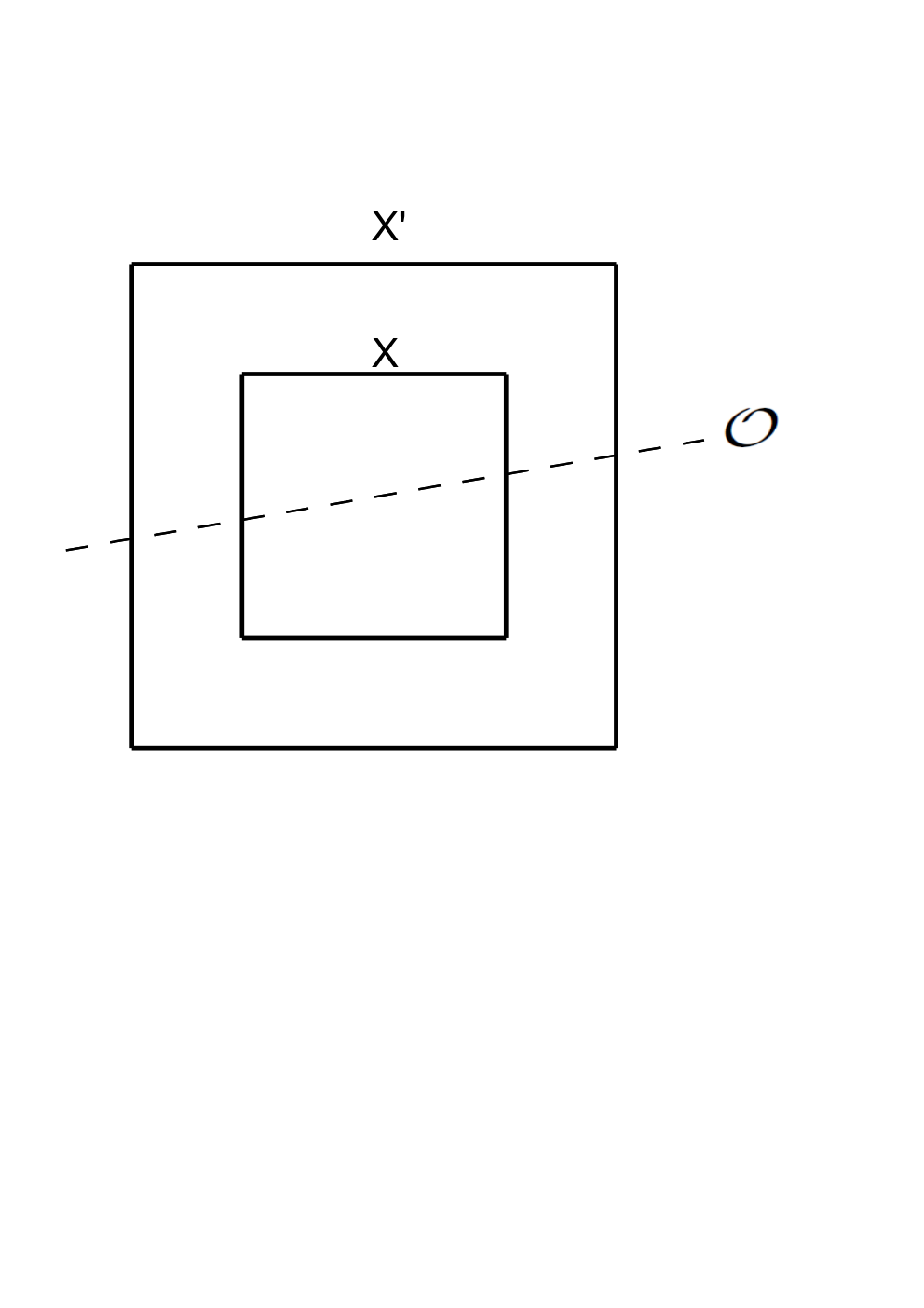
The vector field of the system (1) can vanish at any for a proper selection of . In fact, is the set of all possible equilibrium points of (1), i.e. if is an equilibrium of (1) under feedback control, then . It can be shown that is closed and affine. Also, if , then has dimension (Helwa, Broucke, 2013). Similarly to the case of IBC (Helwa, Caines, 2014a), the location of the set with respect to affects RIBC. Thus, in order to simplify our study of RIBC, we classify our study of RIBC into three geometric cases based on the location of with respect to , namely (i) Case (A): , (ii) Case (B): , and (iii) Case (C): but as shown in Figure 2.


4.1
This geometric situation is shown in Figure 2(a). For this case, the following result shows that the affine system (1) is not RIBC w.r.t. through .
Theorem 4.1
PROOF.
The proof is similar to the proof of Theorem 3.1 of (Helwa, Caines, 2014a). We provide a brief sketch of it in the appendix for completeness of this draft version of the paper.
4.2
This geometric situation is shown in Figure 2(b). For this case, select , and let be such that . This is always possible since . Define and . The dynamics in the new coordinates are . Therefore, for this geometric case, we can assume w.l.o.g. that we study conditions for RIBC of the linear system (2) w.r.t. a polytope through a polytope such that .
Theorem 4.2
PROOF.
The proof is the same as the proof of Theorem 4.1 of (Helwa, Caines, 2014a). A sketch of the proof is provided in the appendix for completeness of this draft version.
Next, we present a second necessary condition for RIBC in this case. To that end, for a convex compact set , we say that the invariance conditions of are solvable (w.r.t. the system (2)) if for each , there exists such that , the Bouligand tangent cone to at (Notice that if is an -dimensional polytope, then , which is defined in the previous section).
Theorem 4.3
PROOF.
By assumption, for each , there exists a state trajectory that connects to in finite time through . Therefore, we have . Since is convex, then we have
Now we show for each , there exist and a control input defined on such that (where is as defined in Definition 4.1), for all , and . This is obvious for points in . For , let and denote the time of reaching the origin and the uniformly bounded control input achieving that, respectively. Then, consider an arbitrary point , . By the definition of the convex hull, there exist points such that , where and . By Caratheodory’s Theorem (Theorem 17.1 of (Rockafellar, 1970)), we know that w.l.o.g. . Let . For each , define the control sequence as follows: for all , and for all . The control sequence drives the system from to in finite time through , then keeps the system at till time . Now starting at , apply the control sequence , for all . Since (2) is linear, it can be shown by a standard argument that the control inputs drive the system from to in finite time through . Also, since for all , we have for all .
Next, let . Clearly, is convex and closed. Then, since , , so is bounded, hence compact. Also, since , is an -dimensional set. It remains to show that the invariance conditions of are solvable. Aided with the property proved in the previous paragraph, this can be shown from the proof of Theorem 4.3 and Remark 4.2 of (Helwa, Caines, 2014a).
Remark 4.1.
If a polytope is given, then checking its invariance conditions is reduced to solving LP problems at the vertices of the given polytope. However, finding a polytope such that its invariance conditions are solvable requires, in general, solving bilinear matrix inequalities (BMIs) (Blanchini, 1999), the solving of which is NP-hard (Toker, Ozbay, 1995). Since the construction of the polytopes satisfying the invariance conditions is carried out offline, available software packages for solving BMIs such as PENBMI (Henrion et al., 2005) can be utilized. There is also a wide literature on constructing polytopic invariant sets (Blanchini, 1999). Instead, note that for (2), is a subspace. If , then one can systematically construct an invariant polytope containing the given polytope , without the need for solving BMIs. Assume w.l.o.g. that the the invariance conditions of are not solvable at the vertices . For a vertex of , , express it as , where and , which is always possible since . Let , for some . Since is affine, . Define , where are the vertices of . By construction, , and it can be shown that . Now we show the invariance conditions of are solvable. At the vertices , select control inputs satisfying the invariance conditions of , and at , select such that , which achieves the invariance conditions at . Finally, at , , since , points toward , and so points inside the interior of the tangent cone to at . Thus, at , , one can always select the control input in the direction of sufficiently large to push the vector field at close enough to , so that it lies in the interior of the tangent cone to at . Instead of the invariant polytopes, one may search for ellipsoidal invariant sets, which are popular candidates since they can be found from the Lyapunov equation or the Ricatti equation (Blanchini, 1999). For instance, one can solve the linear matrix inequalities (LMIs): and . Then, the Lyapunov function is , where , and the corresponding stabilizing feedback is , where (Blanchini, 1999). An invariant ellipsoidal set containing is , where . Examples are provided in Section 5.
We present a third necessary condition for RIBC in this case. For a convex compact set , we say that the backward invariance conditions of are solvable if for each , there exists such that .
Theorem 4.4
PROOF.
By assumption, for each , there exists a state trajectory of (2) that connects to in finite time through . Equivalently, for each , there exists a state trajectory of the backward system that connects to in finite time through . The rest of the proof is the same as the proof of Theorem 4.3 (for the trajectory of the backward system).
Now we present the main result for this geometric case.
Theorem 4.5
Consider the system (2) and -dimensional polytopes such that . If (2) is RIBC w.r.t. through , then the following conditions hold:
- (i)
is controllable.
- (ii)
There exists an -dimensional compact convex set such that and the invariance conditions of are solvable.
- (iii)
There exists an -dimensional compact convex set such that and the backward invariance conditions of are solvable.
Moreover, if are simplicial polytopes, then the conditions (i)-(iii) are also sufficient for RIBC.
PROOF.
The fact that conditions (i)-(iii) are necessary follows directly from Theorems 4.2, 4.3, and 4.4 respectively. Now we prove the sufficiency of (i)-(iii). Since is a simplicial polytope satisfying by assumption, the conditions (i), (ii) imply by Theorem 5.9 of (Helwa, Caines, 2014a) that there exists such that for each , there exist and a control input defined on such that and for all , and . In particular, all the points in can reach in finite time through by applying uniformly bounded control inputs. Then, since is a simplicial polytope satisfying by assumption, the conditions (i), (iii) imply by Theorem 5.10 of (Helwa, Caines, 2014a) that there exists such that for each , there exist and a control input defined on such that and for all , and . In particular, all the points in are accessible from in finite time through by applying uniformly bounded control inputs.
Remark 4.2.
Remark 4.3.
Conditions (i)-(iii) of Theorem 4.5 are also sufficient under other conditions rather than the condition that and are simplicial polytopes. One of these conditions is that and are polytopes, and the strict invariance conditions (strict backward invariance conditions) are solvable for (), respectively. That is to say for each (), there exists such that (), where ((x)) is the interior of the tangent cone to the polytope () at , respectively. The idea of the proof in this case is as follows. First, since the strict invariance conditions of are solvable, one can select a control input at each vertex of satisfying the strict invariance conditions. At , set . Then, triangulate the point set consisting of the vertices of and the origin into -dimensional simplices such that is a vertex in each simplex (always possible since ). See Figure 3.
Using the control inputs selected at the vertices of the simplices of the triangulation, one can construct on each simplex a unique affine feedback such that the overall control law is a continuous piecewise affine (PWA) feedback satisfying the strict invariance conditions of (Habets, van Schuppen, 2004). It is straightforward to show this feedback stabilizes the origin. Starting from any , one can apply the obtained feedback to steer the system from to a point close to in finite time through . Then, from this point, one can use the feedback in Theorem 5.8 of (Helwa, Caines, 2014a) to reach in finite time through . A similar proof can be provided for the backward dynamics to show that from the origin, the system can be steered to any in finite time through . Another condition under which the conditions (i)-(iii) of Theorem 4.5 are sufficient for RIBC is that and are positive invariant ellipsoidal sets associated with Lyapunov functions for the system (2) and the backward dynamics, respectively. An example is given in Section 5 (Example 5.3). For the proof in this case, one can use the stabilizing feedback associated with the Lyapunov function instead of the continuous PWA feedback in the first part of this remark.
Example 4.1.
Consider again the system and the polytope in Example 3.1. We have shown that system (3) is not IBC w.r.t. in this example. Now it is required to check whether (3) is RIBC w.r.t. through .
First, in this example, , the -axis. Clearly, (Case B). We already verified in Example 3.1 that is controllable. Next, we check solvability of the invariance conditions of . By solving an LP program at each vertex of , we find that , and achieve the invariance conditions of at the vertices. As discussed before, this implies the invariance conditions of are solvable (Habets, van Schuppen, 2004). Therefore, condition (ii) of Theorem 4.5 is achieved with . Then, as shown in Example 3.1, the backward invariance conditions of are not solvable. Hence, we search for a simplicial polytope such that and the backward invariance conditions of are solvable. Here . Following Remark 4.1, we find that and . Then, we define . By solving an LP at each vertex of , one can verify that , and satisfy the backward invariance conditions of . Thus, condition (iii) of Theorem 4.5 is achieved with . We conclude from Theorem 4.5 that (3) is RIBC w.r.t. through .
4.3 but
This geometric situation is shown in Figure 2(c). Since , this geometric case is considerably more difficult. For instance, here it is not possible to simplify the problem to studying a linear system on a polytope satisfying , and so some simple proofs of the previous case do not work. Instead, using more involved proofs, we identify conditions for RIBC in this case. We start by showing that controllability of is a necessary condition for RIBC.
Theorem 4.6
PROOF.
Let , and let be such that . Define and . Then, it is easy to verify that the dynamics in the new coordinates are . Let , represent the polytopes expressed in the new coordinates, respectively. It is clear that and . Now suppose by the way of contradiction that is not controllable. Let , where form a basis for the controllability subspace ( is the controllability matrix), and form a basis for . Then, let . The dynamics in the new coordinates are:
| (5) |
where , , , , , and . Let denote the polytopes expressed in the new coordinates. Clearly, and . By assumption, any two states are mutually accessible through . We study all the possible cases of the eigenvalues of , and for each case, we reach a contradiction.
- (i)
The subsystem is unstable: Let be arbitrary. By assumption, there exist bounded control inputs that connect to in finite time through . Also, there exist bounded control inputs that connect to in finite time through . Therefore, starting at , the state trajectory , , can be bounded by a proper selection of . This can only happen if has zero components in the directions of the eigenvectors associated with the unstable eigenvalues of . But since is arbitrary, then it must be that all points in have zero components in the directions of the eigenvectors associated with the unstable eigenvalues of , which clearly contradicts the fact that .
- (ii)
The matrix has an eigenvalue with a negative real part: Similar to the previous case, it can be shown that starting from any , the state trajectory of the backward dynamics can be bounded by a proper selection of . But, this is impossible since the backward dynamics have an uncontrollable eigenvalue with a positive real part (an eigenvalue of the matrix ), and so similar to the previous case, we reach a contradiction.
- (iii)
The matrix has an eigenvalue : By converting the dynamics to the Jordan form, it can be shown there exists such that for any and any . Therefore, starting at any , the state trajectory has a fixed -component whatever control input is selected. Then, since is an -dimensional polytope, there exists such that . This implies is not accessible from whatever control input is selected, a contradiction.
- (iv)
All the eigenvalues of are complex with zero real part: For the repeated eigenvalues, we assume that the associated eigenvectors are linearly independent. For otherwise, the subsystem is unstable (Case (i) of the proof). Then, by a standard argument, there exist two perpendicular directions such that constant, for all , where denotes the state trajectory of (5) under some control input starting at a point . Let be such that . This is always possible since is an -dimensional polytope. Also, since , there exists such that . Now, define , where is selected sufficiently large such that , and the -components of and have the same sign. Then, since are perpendicular, . Thus, the value of evaluated at is different from its value at . Hence, starting at , the state trajectory cannot reach , a contradiction.
Since in all the above cases we reach a contradiction, we conclude that is controllable.
Next, we present a second necessary condition for RIBC in this case. Recall that for system (1) on a compact convex set , we say the invariance conditions of are solvable if for each , there exists such that , and we say the backward invariance conditions of are solvable if for each , there exists such that .
Theorem 4.7
Consider the affine control system (1) and -dimensional polytopes such that , , and . If (1) is RIBC w.r.t. through , then there exists an -dimensional compact convex set such that (i) , (ii) , (iii) the invariance conditions of are solvable, and (iv) the backward invariance conditions of are solvable.
PROOF.
By assumption, there exists such that for every , there exist and a control input defined on such that and for all , and . Therefore, we have
Since is convex, then we have
Let . First, we claim that . For if not, then it can be shown using an argument similar to the proof of Theorem 4.1 that states of are not mutually accessible through , a contradiction. Second, let , and let be such that . This is always possible since . Define and . The dynamics in the new coordinates are . Let , and denote the representations of the sets , and in the new coordinates, respectively. Clearly, and . Also, we have .
Next, we show there exists such that for each , there exists a control input such that and for all . For , the state trajectory can remain in for all by applying the uniformly bounded control inputs that connect to a point in , say , through , and then from apply the uniformly bounded control inputs that connect to through , and repeat this procedure for all future time. Instead, if but , then using an argument similar to the one used in the proof of Theorem 4.3, there exists a control input such that (where is as defined in Definition 4.1) and for all . Using a similar argument, it can be also shown that there exists such that for each , there exists a control input such that and the state trajectory of the backward dynamics , denoted , satisfies for all .
Now let . Clearly, is convex and closed. Also, since , then , and so is bounded, hence compact. Moreover, , and so is an -dimensional set. Furthermore, , and so . Next, we need to show that the invariance conditions of are solvable. Aided with the property proved in the previous paragraph, this follows from the proof of Theorem 4.3 and Remark 4.2 of (Helwa, Caines, 2014a). Similarly, the invariance conditions of w.r.t. the backward dynamics (the backward invariance conditions) can be proved. We conclude is an -dimensional compact convex set satisfying the conditions (i)-(iv) of the theorem.
Now we present the main result for this geometric case.
Theorem 4.8
Consider the affine control system (1) and -dimensional polytopes such that , , and . If (1) is RIBC w.r.t. through , then the following conditions hold:
- (i)
is controllable.
- (ii)
There exists an -dimensional convex compact set such that , and the invariance conditions of are solvable.
- (iii)
There exists an -dimensional convex compact set such that , and the backward invariance conditions of are solvable.
- (iv)
The sets and in conditions (ii), (iii) satisfy .
Moreover, if are simplicial polytopes, then the conditions (i)-(iv) are also sufficient for RIBC.
PROOF.
The necessity of (i) follows from Theorem 4.6. Then, the necessity of (ii)-(iv) follows from Theorem 4.7 (Notice that in Theorem 4.7, and ). Then, assume the conditions (i)-(iv) are achieved, and are simplicial polytopes. We need to show (1) is RIBC w.r.t. through . Let , and let be such that . This is possible since . Define and . The dynamics in the new coordinates are . Let , and represent the sets , and expressed in the new coordinates, respectively. Clearly, , , and . The rest of the proof is the same as the proof of the sufficiency part of Theorem 4.5.
Similarly to Remark 4.3, it can be verified that conditions (i)-(iv) of Theorem 4.8 are also sufficient under the conditions mentioned in Remark 4.3.
Remark 4.4.
Example 4.2.

It is required to study whether (6) is RIBC w.r.t. through . First, we calculate the set of possible equilibria . We have , the axis. Thus, in this example but (Case C). Next, it can be easily verified that is controllable. Now let , and . Then, let . Clearly, . By solving an LP program at each vertex of , we find that the control inputs , and satisfy the invariance conditions of at the vertices. Thus, the invariance conditions of are solvable (Habets, van Schuppen, 2004). Similarly, it can be shown the backward invariance conditions of are solvable. Therefore, the conditions (i)-(iv) of Theorem 4.8 are achieved (with ). We conclude from Theorem 4.8 that (6) is RIBC w.r.t. through in this example.
5 Examples
In this section, we provide three examples to show the motivations behind the relaxed IBC notion, and to clarify the main results of the paper.
Example 5.1.
Consider a cart moving on a bounded table. Let denote the position of the cart, denote the input force, denote the mass of the cart, and denote the coefficient of friction. The state space model of the system is:
| (7) |
Suppose that in this example, we have strict safety constraints: , that should not be violated even in the transient period. These safety constraints define the polytope shown in Figure 5, where , , , and .

In the presence of these strict safety constraints, Kalman’s controllability cannot be used to study mutual accessibility of states. Instead, we first study IBC of the system w.r.t. .
Although is controllable, at the vertex , we have , and , where , whatever is selected. Thus, the invariance conditions of are not solvable at , and from Theorem 3.1, the system is not IBC w.r.t. .
Next, we relax our control objective as follows. Suppose that the nominal operation of the system requires the soft constraints and , resulting in the polytope shown in Figure 5, where , , , and . Starting from any initial position and speed in , can we reach any final position and speed in , without violating the strict safety constraints (through )? To that end, we study relaxed IBC of the system w.r.t. through . In this example, we have and . Hence, (Case B). Since is controllable, it remains to identify the sets in Theorem 4.5 to show relaxed IBC. Notice that , and so . By following the procedure in the first part of Remark 4.1, we construct the invariant polyope , where and . One can also verify that the backward invariance conditions of are solvable. So, we have , and from Theorem 4.5, the system is relaxed IBC w.r.t. through .
Example 5.2.
We consider the mechanical system shown in Figure 6, in which we balance the center of mass above a pivot point.
Examples of balance systems may include persons balancing sticks on their hands, humans standing upright, personal transporters, and rockets, among others (Astrom, Murray, 2008). Let and denote the position and velocity of the cart, respectively, while and denote the angle and angular rate of the structure above the cart, respectively. Assuming that and are close to zero, a linearized model of the system is (Astrom, Murray, 2008)
| (8) |
where is the mass of the cart, and are the moment of inertia and the mass of the system to be balanced, respectively, is the distance between the cart and the center of mass of the balanced body, is the gravitational acceleration constant (), and , are coefficients of viscous friction. Also, is the total inertia, is the total mass, and . Now suppose that it is required to study whether we can mutually connect the states of the system having positive angle , without changing the sign of the angle . In particular, it is required to study mutual accessibility of the states in
through
To that end, we study relaxed IBC of the system w.r.t. through . First, we calculate the set of possible equilibria . In this example, it can be verified that , the -axis, and that (Case A). From Theorem 4.1, the system is not relaxed IBC w.r.t. through . To clarify more the obtained conclusion, let . It can be verified that , i.e. , and . Since it is always the case that , then , for all . Thus, starting at a point , the -component of the state trajectory is non-increasing as long as is non-negative, whatever is selected. In particular, let and . We have , and so starting from , we cannot reach through . This clarifies the proof of Theorem 4.1.
Example 5.3.
Consider the linear circuit, shown in Figure 7, where , , and .
The state space model of the system is
| (9) |
Let , and . It is required to study mutual accessibility of the states of through . First, we calculate the set of possible equilibria . We have (Case B). Second, it is easy to verify that is controllable. Third, we identify a convex, compact set such that , and the invariance conditions of are solvable. Following Remark 4.1, we solve a set of LMIs to get a stabilizing feedback and a corresponding Lyapunov function. We find that , and the Lyapunov function is , where
Let . It can be verified that the compact, convex set satisfies , and satisfies the invariance conditions of . Next, we identify a convex, compact set such that , and the backward invariance conditions of are solvable. Following Remark 4.1, we solve a set of LMIs to get a stabilizing feedback for the backward dynamics and a corresponding Lyapunov function. We find , and the Lyapunov function for the backward dynamics is , where
Let . It can be verified that the compact, convex set satisfies , and satisfies the backward invariance conditions of . Collecting all of the above together, we conclude from Theorem 4.5 that the system is relaxed IBC w.r.t. through .
For instance, suppose that it is required to connect to in finite time through .
Figure 8(a) shows the trajectory obtained by applying the traditional control law (10), where . One can see that the trajectory reaches the point , outside , which means it violates the strict safety constraints in this example. Instead, by following our proposed method in Remark 4.3, we first apply the control law to steer the system to a point near the origin through (the blue trajectory), then use the control law (10) to connect the points close to the origin through (the green trajectory), and finally apply to steer the system to through (the red trajectory). See Figure 8(b).
6 Conclusion
In this paper, we have extended the results of (Helwa, Caines, 2014a; Helwa, Caines, 2016) by studying the case where the given affine system is not in-block controllable with respect to the given polytope. In particular, we have introduced the notion of relaxed in-block controllability (RIBC) which studies mutual accessibility of the states in the interior of a given polytope through the interior of a given bigger polytope by applying uniformly bounded control inputs. By exploring all the possible geometric cases, we have provided necessary conditions for RIBC in all these cases. Moreover, we have shown when these conditions are also sufficient. Several examples have been provided to clarify the main results of the paper.
Appendix
This appendix contains proofs included in this draft version for completeness.
Proof of Lemma 3.2:
Let be arbitrary. Since is controllable, it is well known that for any , is invertible, and the control input
| (10) |
steers the system from to in finite time . Since is compact, exists, and so we can always identify a uniform upper bound such that for all . By a straightforward argument, it can be shown that under (10), there exists a uniform such that for all .
Proof of Theorem 4.1:
Since , then by Lemma 4.1 of (Helwa, Broucke, 2013), there exists , the perpendicular subspace to , such that , for all and all . This implies for any and under any control input, is non-increasing as long as . Then since is an n-dimensional polytope, we can identify two points such that . Clearly, starting from , the system cannot reach through .
References
- Alexis et al. (2011) Alexis K., Nikolakopoulos G., Tzes A. (2011). Switching model predictive attitude control for a quadrotor helicopter subject to atmospheric disturbances. Control Engineering Practice. Vol. 19(10), pp. 1195 - 1207.
- Alizadeh et al. (2014) Alizadeh H. V., Helwa M. K., Boulet B. (2014). Constrained control of the synchromesh operating state in an electric vehicle’s clutchless automated manual transmission. IEEE Conference on Control Applications, Antibes, France, pp. 623 - 628.
- Astrom, Murray (2008) Astrom K. J., Murray R. M (2008). Feedback Systems. Princeton University Press, Princeton, New Jersey.
- Barvinok (2013) Barvinok A. (2013). Thrifty Approximations of Convex Bodies by Polytopes. Int. Math. Research Notices. Published online.
- Bemporad, Morari (1999) Bemporad A., Morari M. (1999). Control of systems integrating logic, dynamics, and constraints. Automatica. Vol. 35, pp. 407-428.
- Bemporad et al. (2000) Bemporad A., Ferrari-Trecate G., Morari M. (2000). Observability and controllability of piecewise affine and hybrid systems. IEEE Trans. Automatic Control. Vol. 45(10), pp. 1864-1876.
- Blanchini (1999) Blanchini F. (1999). Set invariance in control. Automatica. Vol. 35, pp. 1747-1767.
- Blanchini, Miani (2008) Blanchini F., Miani S. (2008). Set-Theoretic Methods in Control. Birkhauser Boston.
- Borrelli et al. (2006) Borrelli F., Bemporad A., Fodor M., Hrovat D. (2006). An MPC/hybrid system approach to traction control. IEEE Transactions on Control Systems Technology. Vol. 14(3), pp. 541 - 552.
- Brammer (1972) Brammer R.F. (1972). Controllability in linear autonomous systems with positive controllers. SIAM Journal on Control. Vol. 10(2), pp. 339-353.
- Brondsted (1983) Brondsted A. (1983) An Introduction to Convex Polytopes. Springer-Verlag, New York Inc.
- Broucke (2010) Broucke M.E. (2010) Reach control on simplices by continuous state feedback. SIAM Journal on Control and Optimization. Vol. 48 (5), pp. 3482-3500.
- Caines, Shaikh (2008) Caines P.E., Shahid Shaikh M. (2006). Optimality zone algorithms for hybrid systems: efficient algorithms for optimal location and control computation. Hybrid Systems: Computation and Control, Lecture Notes in Computer Science, Vol. 3927, pp. 123-137.
- Caines, Wei (1995) Caines P. E. and Wei Y. J. (1995). The Hierarchical Lattices of a Finite Machine. Systems and Control Letters. Vol. 25, pp. 257-263.
- Caines, Wei (1998) Caines P.E. and Wei Y.J. (1998). Hierarchical Hybrid Control Systems: A Lattice Theoretic Formulation. IEEE Transactions on Automatic Control. Vol. 43 (4), pp. 501-508.
- Clarke et al. (1998) Clarke F. H., Ledyaev Y. S., Stern R. J., Wolenski P. R. (1998) Nonsmooth Analysis and Control Theory. Springer-Verlag New York Inc..
- Filippov (1988) Filippov A. F. (1988). Differential Equations with Discontinuous Right Hand Sides. Kluwer Academic Publishers.
- Geyer et al. (2005) Geyer T., Papafotion G., Morari M. (2005). Model predictive control in power electronics: a hybrid systems approach. The 44th IEEE Conference on Decision and Control, and the European Control conference, Seville, Spain, pp. 5606 - 5611.
- Girard, Pappas (2007) Girard A., Pappas G. (2007). Approximate bisimulation relations for constrained linear systems. Automatica, Vol. 43(8), pp. 1307-1317.
- Goebel et al. (2009) Goebel R., Sanfelice R. G., and Teel A. R. (2009). Hybrid dynamical systems. IEEE Control Systems Magazine. Vol. 29 (2), pp. 28–93.
- Habets, van Schuppen (2004) Habets L.C.G.J.M., van Schuppen J.H. (2004). A control problem for affine dynamical systems on a full-dimensional polytope. Automatica, 40(1), pp. 21–35.
- Habets et al. (2006) Habets L.C.G.J.M.,Collins P.J., van Schuppen J.H. (2006). Reachability and control synthesis for piecewise-affine hybrid systems on simplices. IEEE Trans. Automatic Control. Vol. 51 (6), pp. 938–948.
- Heemels, Camlibel (2007) Heemels W.P.M.H., Camlibel M.K. (2007). Controllability of linear systems with input and state constraints. The 46th IEEE Conference on Decision and Control(CDC), New Orleans, pp. 536-541.
- Heemels, Camlibel (2008) Heemels W.P.M.H., Camlibel M.K. (2008). Null controllability of discrete-time linear systems with input and state constraints. The 47th Conference on Decision and Control(CDC), Cancun, Mexico, pp. 3487-3492.
- Helwa (2013) Helwa M. (2013). Reach Control Problems on Polytopes. PhD thesis, University of Toronto.
- Helwa (2015) Helwa M. K. (2015). In-block controllability of controlled switched linear systems on polytopes. IFAC-Papers OnLine, Elsevier. Vol. 48 (27), pp. 7-12.
- Helwa, Broucke (2012) Helwa M.K., Broucke M.E. (2012). Generalized flow conditions for reach control on polytopes. Proceedings of the 51st IEEE Conference on Decision and Control. Maui, Hawaii, pp. 4199-4204.
- Helwa, Broucke (2013) Helwa M.K., Broucke M.E. (2013). Monotonic Reach Control on Polytopes. IEEE Transactions on Automatic Control. Vol. 58 (10), pp. 2704–2709.
- Helwa, Broucke (2014) Helwa M.K., Broucke M.E. (2014). Reach control of single-input systems on simplices using multi-affine feedback. The 21st International Symposium on Mathematical Theory of Networks and Systems, Groningen, Netherlands.
- Helwa, Broucke (2015) Helwa M.K., Broucke M.E. (2015). Flow functions, control flow functions, and the reach control problem. Automatica. Vol. 55, pp. 108 - 115.
- Helwa et al. (2016) Helwa M.K., Lin Z., Broucke M.E. (2016). On the necessity of the invariance conditions for reach control on polytopes. Systems and Control Letters. Vol. 90, pp. 16 - 19.
- Helwa, Caines (2014a) Helwa M.K., Caines P.E. (2014a). In-Block Controllability of Affine Systems on Polytopes. Proceedings of the 53rd Conference on Decision and Control, Los Angeles, pp. 3936-3942.
- Helwa, Caines (2014b) Helwa M.K., Caines P.E. (2014b). Relaxed In-Block Controllability of Affine Systems on Polytopes. Proceedings of the 53rd Conference on Decision and Control, Los Angeles, Dec 2014, pp. 3943-3949.
- Helwa, Caines (2014c) Helwa M.K., Caines P.E. (2014c). Hierarchical Control of Piecewise Affine Hybrid Systems. Proceedings of the 53rd Conference on Decision and Control, Los Angeles, Dec 2014, pp. 3950-3956.
- Helwa, Caines (2015a) Helwa M.K., Caines P.E. (2015a). Epsilon controllability of nonlinear systems on polytopes. The 54rd Conf. on Decision and Control, Osaka, Japan, pp. 252-257.
- Helwa, Caines (2015b) Helwa M. K., Caines P. E. (2015b). On the construction of in-block controllable covers of nonlinear systems on polytopes. IEEE Conference on Decision and Control, Osaka, pp. 276-281.
- Helwa, Caines (2016) Helwa M.K., Caines P.E. (2016). In-Block Controllability of Affine Systems on Polytopes. IEEE Transactions on Automatic Control, accepted.
- Helwa, Schoellig (2016) Helwa M. K., Schoellig A. P. (2016). On the construction of safe controllable regions for affine systems with applications to robotics. IEEE Conference on Decision and Control, Las Vegas, accepted.
- Henrion et al. (2005) Henrion D., Lofberg J., Kocvara M., Stingl M. (2008). Solving polynomial static output feedback problems with PENBMI. The 44th IEEE Conf. Dec. and Con., and the Eur. Con. Conf. Seville, pp. 7581-7586.
- Hopcroft, Ullman (1979) Hopcroft J., Ullman J. (1979). Introduction to Automata Theory, Languages, and Computation. Addison-Wesley.
- Hubbard, Caines (2002) Hubbard P., Caines P.E. (2002). Dynamical Consistency in Hierarchical Supervisory Control. IEEE Transactions on Automatic Control, Vol. 47 (1), pp 37 - 52.
- Juloski et al. (2005) Juloski A. L., Heemels W., Ferrari-Trecate G., Vidal R., Paoletti S., and Niessen J. (2005) Comparison of four procedures for the identification of hybrid systems. Hybrid Systems: Computation and Control. Vol. 3414, pp. 354-369.
- Kalman (1960) Kalman R. E. (1960). On the general theory of control systems. The 1st World Congress of the International Federation of Automatic Control, pp. 481-493.
- Moreno, Schneider (2007) Moreno J. P., Schneider R. (2007). Intersection properties of polyhedral norms. Advances in Geometry. Vol. 7 (3), pp. 391-402.
- Rockafellar (1970) Rockafellar R.T. (1970). Convex Analysis. Princeton University Press, Princeton, New Jersey.
- Rodrigues, Boyd (2005) Rodrigues L., Boyd S. (2005). Piecewise-affine state feedback for piecewise-affine slab systems using convex optimization. Sys. and Con. Let. Vol. 54(9), pp. 835-853.
- Schoellig et al. (2007) Schoellig A., Caines P. E., Egerstedt M., Malham E. (2007). A hybrid Bellman equation for systems with regional dynamics. The 46th Conference on Decision and Control(CDC), New Orleans, pp. 3393-3398.
- Sontag (1984) Sontag E.D. (1984). An algebraic approach to bounded controllability of linear systems. International Journal of Control. Vol. 39 (1), pp. 181-188.
- Toker, Ozbay (1995) Toker O., Ozbay H. (1995). On the NP-hardness of solving bilinear matrix inequalities and simultaneous stabilization with static output feedback. The American Control Conference, Seattle, USA, pp. 2525-2526.
- Yordanov et al. (2010) Yordanov B., Tumova J., Belta C., Cerna I., Barnat J. (2010). Formal analysis of piecewise affine systems through formula guided refinement. The 49th IEEE Conference on Decision and Control. Atlanta, pp. 5899-5904.
- Zamani et al. (2012) Zamani M., Pola G., Mazo Jr. M., and Tabuada P. (2012) Symbolic models for nonlinear control systems without stability assumptions. IEEE Trans. Automat. Control, vol. 57, no. 7, pp. 1804–1809.